Resistivity mapping with GEOPHILUS ELECTRICUS ... · Resistivity mapping with GEOPHILUS ELECTRICUS — Information about lateral and vertical soil heterogeneity E. Lueck a,⁎, J

Geoderma xxx (2012) xxx–xxx

GEODER-11201; No of Pages 10

Contents lists available at SciVerse ScienceDirect

Geoderma

j ourna l homepage: www.e lsev ie r .com/ locate /geoderma

Resistivity mapping with GEOPHILUS ELECTRICUS — Information about lateral andvertical soil heterogeneity

E. Lueck a,⁎, J. Ruehlmann b

a University of Potsdam, Institute of Earth- and Environmental Science, Karl-Liebknecht-Str. 24, 14476 Potsdam, Germanyb Leibniz-Institute of Vegetable and Ornamental Crops, Theodor-Echtermeyer-Weg 1, 14979 Grossbeeren, Germany

⁎ Corresponding author. Tel.: +49 331 977 5781; faxE-mail address: [email protected] (E. Luec

0016-7061/$ – see front matter © 2012 Published by Elhttp://dx.doi.org/10.1016/j.geoderma.2012.11.009

Please cite this article as: Lueck, E., Ruehlmanheterogeneity, Geoderma (2012), http://dx.d

a b s t r a c t
a r t i c l e i n f o
Article history:Received 8 September 2011Received in revised form 6 November 2012Accepted 7 November 2012Available online xxxx

Keywords:Proximal soil sensingElectrical conductivityElectrical resistivityPhase angleMappingSoil stratification

GEOPHILUS ELECTRICUS (nickname GEOPHILUS) is a novel system for mapping the complex electrical bulkresistivity of soils. Rolling electrodes simultaneously measure amplitude and phase data at frequencies rang-ing from 1 mHz to 1 kHz. The sensor's design and technical specifications allow for measuring these param-eters at five depths of up to ca. 1.5 m. Data inversion techniques can be employed to determine resistivitymodels instead of apparent values and to image soil layers and their geometry with depth. When used incombination with a global positioning system (GPS) and a suitable cross-country vehicle, it is possible tomap about 100 ha/day (assuming 1 data point is recorded per second and the line spacing is 18 m). The ap-plicability of the GEOPHILUS system has been demonstrated on several sites, where soils show variations intexture, stratification, and thus electrical characteristics. The data quality has been studied by comparisonwith ‘static’ electrodes, by repeated measurements, and by comparison with other mobile conductivity map-ping devices (VERIS3100 and EM38). The high quality of the conductivity data produced by the GEOPHILUSsystem is evident and demonstrated by the overall consistency of the individual maps, and in the clear strat-ification also confirmed by independent data.The GEOPHILUS system measures complex values of electrical resistivity in terms of amplitude and phase.Whereas electrical conductivity data (amplitude) are well established in soil science, the interpretation ofphase data is a topic of current research. Whether phase data are able to provide additional information de-pends on the site-specific settings. Here, we present examples, where phase data provide complementary in-formation on man-made structures such as metal pipes and soil compaction.

© 2012 Published by Elsevier B.V.

1. Introduction

Proximal soil sensing involves the application of a range of instru-ments employing several methods and techniques to map soil struc-tures and characteristics at its surface (Adamchuk and ViscarraRossel, 2011; Mahmood et al., 2012; Viscarra Rossel et al., 2010).Methods involving measurements of apparent electrical conductivity(ECa) and its reciprocal, apparent electrical resistivity (ρa), representpopular approaches and still hold promise for future developments(Allred et al., 2008; Corwin and Lesch, 2005; Saey et al., 2009;Samouёlian et al., 2005; Sudduth et al., 2003). Such conductivity map-ping approaches increasingly use mobile sensors in combination withGPS technology. Generally, three main groups of soil conductivitymeasurement approaches can be distinguished — direct current(DC) methods, electromagnetic methods (EM) and method workingwith capacitively-coupled electrodes. In each case the data and thespatial resolution vary depending on the specific method applied. Ca-pacitive methods operate over high resistive ground where grounded

: +49 331 977 5700.k).

sevier B.V.

n, J., Resistivity mapping withoi.org/10.1016/j.geoderma.20

measurements are difficult to realize (Kuras et al., 2007; De Pascale etal., 2008). While electromagnetic methods are more sensitive to highlyconductive soils, the DCmethod is more suitable for investigating high-ly resistive soils (Clark, 1997). Technical parameters like the geometrybetween electrodes or coils, the applied frequencies, and the observedtime window, determine the depth of investigation and thereby thesoil volume covered (Pellerin and Wannamaker, 2005). In contrast tothe DC method, the electromagnetic and capacitive methods requireno galvanic coupling between the sensor and the soil. The electromag-netic methods deal with phenomena of electromagnetic induction(EMI) and have, compared to the DC method, the advantage that themeasurement equipment is lighter in weight, smaller in size, and thuseasier to handle. On the other hand, theDCmethodshave the advantagethat i) they do not require instrument calibration at the beginning of asurvey and therefore produce absolute resistivity data and that ii) dif-ferent andflexible electrode configurations can be employed. For exam-ple, varying the spacing between individual electrodes effects the depthrange and sensitivity-depth-functions.

Further measurement principles, such as the induced-polarization(IP) and the spectral induced polarization (SIP) method were mainlydeveloped for the prospection of mineral deposits, but they are only

GEOPHILUS ELECTRICUS— Information about lateral and vertical soil12.11.009

http://dx.doi.org/10.1016/j.geoderma.2012.11.009

mailto:[email protected]


http://www.sciencedirect.com/science/journal/00167061


Table 1Technical specifications of the GEOPHILUS system.

Electrode configurationType of array Equatorial Dipole–Dipole-ArrayNumber of dipoles 6 (1 transmitter, 5 receiver dipoles)Dipole length 1 mDipole spacing 0.5, 1.0, 1.5, 2.0 and 2.5 m

Transmitter specificationsOutput power 50 WOutput voltage up to±400 VOutput current up to±250 mASignal frequencies 1 mHz–1 kHzNumber of simultaneous usedfrequencies

4

Preferred frequencies 62.5, 125, 187.5 and 562.5 HzReceiver specifications

A/D converter 24 BitInput range ±2 VInput Impedance and capacity >1 GΩ, 6 pFDynamic range >120 dBSampling rate 0.9 sMeasured values Complex resistivity

(absolute value and phase)

2 E. Lueck, J. Ruehlmann / Geoderma xxx (2012) xxx–xxx

rarely considered in proximal soil sensing. In recent years, the numberof studies concerning the application of IP and SIP has increased innear-surface geophysics. However, using these techniques in soil sci-ences is relatively new. Laboratory measurements, field and modelingstudies are used to clarify data produced by IP and SIP methods. Whilethe electrical conductivity of soils is strongly influenced by soil mois-ture, polarization effects are influenced by pore structure (Binley etal., 2005) as well as by pore fluid and salt concentration (Lesmes andFrye, 2001). Microscopic polarization effects depending on structureand electrolyte properties result in a phase shift between current andvoltage and finally in a frequency dependence of ECa.

If soil mapping based on geophysical measurementmethods shouldbecome attractive for applications on large spatial scales, mobile mea-surement techniques (on-the-go sensors) are required. The idea to pro-ducemobilized resistivity sensors (rolling or towed electrodes) in orderto enable large areas to be surveyed has existed for more than 70 years(Jakosky, 1938). Since then, several technical solutions have becomeavailable on the market. In 1972, a prototype of a wheeled resistivityarray (twin electrode) was suggested by A. Clark from The School of Ar-chaeological Sciences at Bradford University (Clark, 1997). In the 70's,German geophysicists developed towed electrodes and patented thesein 1979 (Jonek et al., 1979). British archaeologists have traditionallypreferred systems which can be moved by hand (Walker and Linford,2006). A motorized system (ARP — automatic resistivity system) has re-cently been developed at the French Centre de Recherches Géophysiques(Dabas, 2009; Panissod et al., 1997). It is now used by the companyGeocarta in archaeological surveys, and also in applications from agricul-ture and viticulture. Similar techniques are available in theUSA fromVerisTechnologies (Lund et al., 1999). Additional to the rolling electrodes, sys-tems with towed electrodes, like PA-CEP from The University of Aarhus(Sørensen, 1996), or with capacitive coupling, like CORIM from IRIS in-struments (France) and the Ohm-Mapper from Geometrics (U.S.A.)have been developed and are now available. The latter are suitable forhighly resistive surfaces but their success on highly conductive soils isdoubtful because of the small signal-to-noise ratio (Gebbers et al., 2009).Applications of mobilized conductivity measurements are not only re-stricted to land but can also be used for the classification of marine sedi-ments (Lavoie et al., 1988).

Regarding their spatial resolution capabilities, most high-resolution soil mapping sensors focus on lateral variations of appar-ent electrical resistivity, but not on the vertical variations (i.e. stratifi-cation). However, not only lateral but also vertical variations of soilproperties have to be considered to describe soil heterogeneity; e.g.stratified soils with undulating layers of different soil textures affectthe hydrological soil properties. Most models assume that either thetopsoil is more or less homogeneous and lateral variations are onlycaused by differences in topsoil thickness or that actually conductivi-ty patterns only reflect topsoil heterogeneity without changes in top-soil thickness. These models can be improved by combining data withdifferent ECa depth-response functions (Sudduth et al., 2010;Tabbagh et al., 2000).

Here, we describe the new sensor GEOPHILUS which was devel-oped to combine advantages of existing sensors as mentioned abovewith the progress in the measurement techniques as well as withthe requirements on a modern on-the-go sensor. Consequently, com-pared to relevant existing sensors the GEOPHILUS measurement sys-tem is characterized by some new features (five channels, fourfrequencies, complex value of resistivity in terms of amplitude andphase) as discussed in more detail below.

Therefore, additionally to providing a general introduction to theGEOPHILUS system, the aim of this publication is

- to demonstrate the temporal stability of resistivity patterns(short-term and long-term),

- to compare the results of GEOPHILUS measurements with those ofwell-established equipment (VERIS3100 and EM38) and

Please cite this article as: Lueck, E., Ruehlmann, J., Resistivity mapping withheterogeneity, Geoderma (2012), http://dx.doi.org/10.1016/j.geoderma.2

- for the first time, to present measurements of certain parameters(soil stratification, multi-frequency, phase) recorded “on-the-go”.

2. Materials and methods

2.1. Technical parameters of the sensor

GEOPHILUS represents a modular system which is compatiblewith several arrays of electrodes. Currently, the system consists ofan equatorial dipole–dipole array (six pairs of galvanic coupling elec-trodes) and a special SIP instrument developed by Radić Research,Germany (Radić, 2007). The time it takes to download the systemfrom the trailer and prepare all components (electrodes, instrumentsand the GPS) corresponds to the warm up time of the electronicequipment which is about 20 min.

The system is capable of recording complex resistivity (absolutevalue and phase) simultaneously for four frequencies within therange of 1 mHz to 1 kHz. All data are averaged over some signal pe-riods. Different statistical measures calculated within these periodsprovide an immediate impression on data quality. Table 1 summa-rizes the most important technical specifications of the GEOPHILUSsystem (Radić, 2005).

The new sensor's design (Fig. 1) and technical specifications (6channels organized by 6 remote units — RU) allow for measuringthe electrical parameters at five depth levels up to a depth of ca.1.5 m. The first remote unit (RU-1) measures the voltage drop acrossa shunt resistance of 7.8 Ω to calculate the injected current. The otherunits (RU2–RU6) measure the voltages. In the following they are re-ferred to as channel 1 to channel 5. For all data presented withinthis publication, an equatorial dipole–dipole-array with a dipolelength of 1 m has been used. The dipole spacing varies between 0.5and 2.5 m with increments of 0.5 m. Increasing channel number cor-responds to increasing dipole spacing; i.e. increasing depth. Thedepth of investigation and sensitivity-depth-curves are comparableto an inline pole–dipole-array of equal size (Butler, 2005).

Increasing the dipole spacing results in a smoothing of the normalizedsensitivity curves and in shifting the maximum sensitivity values to in-creased depths. Channel 1 is mostly influenced by the upper 0.5 m andabout 50% of the signal of channel 5 reflects the depth range between0.25 and 1.5 m. The corresponding sensitivity-depth-curves (Fig. 2)were calculated using the approach of Roy and Apparao (1971).

In addition to the depth of investigation, the dipole spacing alsoinfluences the signal-to-noise ratio of the recorded data. Increaseddistances between current and potential electrodes result in lower



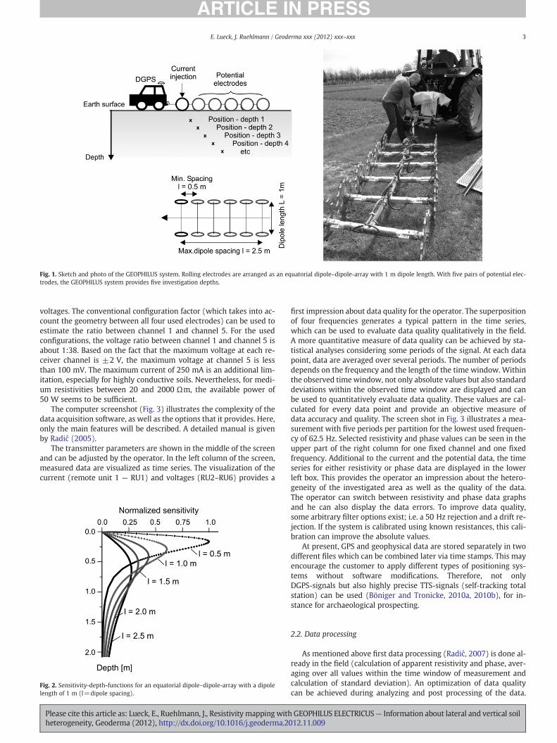
Fig. 1. Sketch and photo of the GEOPHILUS system. Rolling electrodes are arranged as an equatorial dipole–dipole-array with 1 m dipole length. With five pairs of potential elec-trodes, the GEOPHILUS system provides five investigation depths.

3E. Lueck, J. Ruehlmann / Geoderma xxx (2012) xxx–xxx

voltages. The conventional configuration factor (which takes into ac-count the geometry between all four used electrodes) can be used toestimate the ratio between channel 1 and channel 5. For the usedconfigurations, the voltage ratio between channel 1 and channel 5 isabout 1:38. Based on the fact that the maximum voltage at each re-ceiver channel is ±2 V, the maximum voltage at channel 5 is lessthan 100 mV. The maximum current of 250 mA is an additional lim-itation, especially for highly conductive soils. Nevertheless, for medi-um resistivities between 20 and 2000 Ωm, the available power of50 W seems to be sufficient.

The computer screenshot (Fig. 3) illustrates the complexity of thedata acquisition software, as well as the options that it provides. Here,only the main features will be described. A detailed manual is givenby Radić (2005).

The transmitter parameters are shown in the middle of the screenand can be adjusted by the operator. In the left column of the screen,measured data are visualized as time series. The visualization of thecurrent (remote unit 1 — RU1) and voltages (RU2–RU6) provides a

Fig. 2. Sensitivity-depth-functions for an equatorial dipole–dipole-array with a dipolelength of 1 m (l=dipole spacing).


first impression about data quality for the operator. The superpositionof four frequencies generates a typical pattern in the time series,which can be used to evaluate data quality qualitatively in the field.A more quantitative measure of data quality can be achieved by sta-tistical analyses considering some periods of the signal. At each datapoint, data are averaged over several periods. The number of periodsdepends on the frequency and the length of the time window. Withinthe observed timewindow, not only absolute values but also standarddeviations within the observed time window are displayed and canbe used to quantitatively evaluate data quality. These values are cal-culated for every data point and provide an objective measure ofdata accuracy and quality. The screen shot in Fig. 3 illustrates a mea-surement with five periods per partition for the lowest used frequen-cy of 62.5 Hz. Selected resistivity and phase values can be seen in theupper part of the right column for one fixed channel and one fixedfrequency. Additional to the current and the potential data, the timeseries for either resistivity or phase data are displayed in the lowerleft box. This provides the operator an impression about the hetero-geneity of the investigated area as well as the quality of the data.The operator can switch between resistivity and phase data graphsand he can also display the data errors. To improve data quality,some arbitrary filter options exist; i.e. a 50 Hz rejection and a drift re-jection. If the system is calibrated using known resistances, this cali-bration can improve the absolute values.

At present, GPS and geophysical data are stored separately in twodifferent files which can be combined later via time stamps. This mayencourage the customer to apply different types of positioning sys-tems without software modifications. Therefore, not onlyDGPS-signals but also highly precise TTS-signals (self-tracking totalstation) can be used (Böniger and Tronicke, 2010a, 2010b), for in-stance for archaeological prospecting.

2.2. Data processing

As mentioned above first data processing (Radić, 2007) is done al-ready in the field (calculation of apparent resistivity and phase, aver-aging over all values within the time window of measurement andcalculation of standard deviation). An optimization of data qualitycan be achieved during analyzing and post processing of the data.



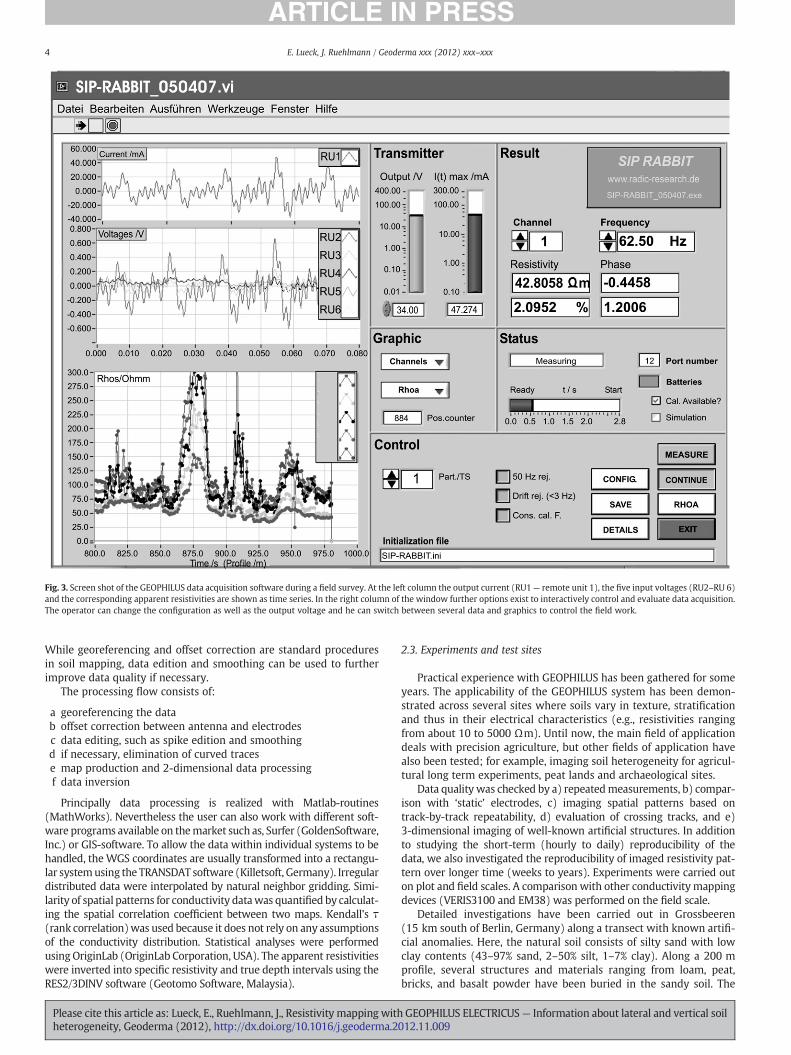
Fig. 3. Screen shot of the GEOPHILUS data acquisition software during a field survey. At the left column the output current (RU1— remote unit 1), the five input voltages (RU2–RU 6)and the corresponding apparent resistivities are shown as time series. In the right column of the window further options exist to interactively control and evaluate data acquisition.The operator can change the configuration as well as the output voltage and he can switch between several data and graphics to control the field work.


While georeferencing and offset correction are standard proceduresin soil mapping, data edition and smoothing can be used to furtherimprove data quality if necessary.

The processing flow consists of:

a georeferencing the datab offset correction between antenna and electrodesc data editing, such as spike edition and smoothingd if necessary, elimination of curved tracese map production and 2-dimensional data processingf data inversion

Principally data processing is realized with Matlab-routines(MathWorks). Nevertheless the user can also work with different soft-ware programs available on themarket such as, Surfer (GoldenSoftware,Inc.) or GIS-software. To allow the data within individual systems to behandled, the WGS coordinates are usually transformed into a rectangu-lar systemusing the TRANSDAT software (Killetsoft, Germany). Irregulardistributed data were interpolated by natural neighbor gridding. Simi-larity of spatial patterns for conductivity datawas quantified by calculat-ing the spatial correlation coefficient between two maps. Kendall's τ(rank correlation)was used because it does not rely on any assumptionsof the conductivity distribution. Statistical analyses were performedusing OriginLab (OriginLab Corporation, USA). The apparent resistivitieswere inverted into specific resistivity and true depth intervals using theRES2/3DINV software (Geotomo Software, Malaysia).


2.3. Experiments and test sites

Practical experience with GEOPHILUS has been gathered for someyears. The applicability of the GEOPHILUS system has been demon-strated across several sites where soils vary in texture, stratificationand thus in their electrical characteristics (e.g., resistivities rangingfrom about 10 to 5000 Ωm). Until now, the main field of applicationdeals with precision agriculture, but other fields of application havealso been tested; for example, imaging soil heterogeneity for agricul-tural long term experiments, peat lands and archaeological sites.

Data quality was checked by a) repeatedmeasurements, b) compar-ison with ‘static’ electrodes, c) imaging spatial patterns based ontrack-by-track repeatability, d) evaluation of crossing tracks, and e)3-dimensional imaging of well-known artificial structures. In additionto studying the short-term (hourly to daily) reproducibility of thedata, we also investigated the reproducibility of imaged resistivity pat-tern over longer time (weeks to years). Experiments were carried outon plot and field scales. A comparison with other conductivitymappingdevices (VERIS3100 and EM38) was performed on the field scale.

Detailed investigations have been carried out in Grossbeeren(15 km south of Berlin, Germany) along a transect with known artifi-cial anomalies. Here, the natural soil consists of silty sand with lowclay contents (43–97% sand, 2–50% silt, 1–7% clay). Along a 200 mprofile, several structures and materials ranging from loam, peat,bricks, and basalt powder have been buried in the sandy soil. The




differences in soil texture generate conductivity contrasts which canbe measured by electrical methods. The structure of an artificialloam body (silt content about 39% and clay content about 8%) willbe discussed in more detail.

The second field site is an experimental farm in Koellitsch (Saxony,Germany) which is located on the floodplain of the river Elbe. The siteis characterized by strong heterogeneities. Here, we find fluviatileloamy sediments on a sandy, unfertile subsoil. The thickness of theloam layer varies from a few centimeters up to more than 1 m. Thefarm in Koellitsch started conductivity mapping 15 years ago. Sensorslike EM38 (430 ha), VERIS-3100 (250 ha) and GEOPHILUS (470 ha)have been tested to evaluate different conductivity methods.

In Horstwalde (about 30 km south of Berlin, Germany) a test site hasbeen established to develop techniques for characterizing near-surfacesedimentary environments. In the development phase of this test site,also GEOPHILUS measurements have been conducted and comparedwith magnetic and electromagnetic (EM38) data. The primary goal ofthese surveys was to detect buried utilities installed during the past cen-tury when the site was used as a military training area (Böniger andTronicke, 2010a). At this site, the local geology is characterized by layeredsequences of sand- and gravel-dominated (clay-free) glaciofluvial sedi-ments (Tronicke et al., 2012).

3. Results

3.1. Temporal stability of resistivity patterns

The investigations regarding the temporal stability of resistivity pat-ternswere divided in two different time ranges investigating short- andlong-term stability of the imaged patterns. The short-term investiga-tions cover a time range of about 1 h and reflectmore technical aspects,e.g. quality of the galvanic coupling between the rolling electrodes andthe soil. In contrast, the investigations concerning the long-term stabil-ity of resistivity patterns were especially affected by changes in soilmoisture, soil temperature, and soil roughness.

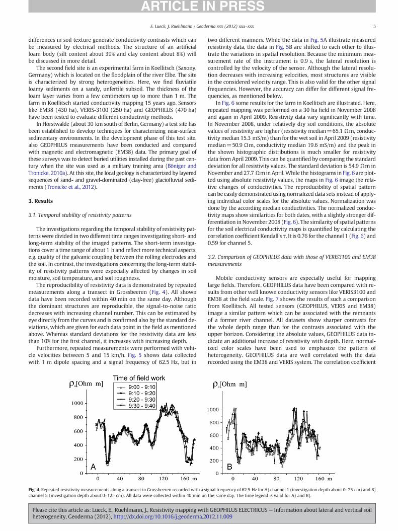
The reproducibility of resistivity data is demonstrated by repeatedmeasurements along a transect in Grossbeeren (Fig. 4). All showndata have been recorded within 40 min on the same day. Althoughthe dominant structures are reproducible, the signal-to-noise ratiodecreases with increasing channel number. This can be estimated byeye directly from the curves and is confirmed also by the standard de-viations, which are given for each data point in the field as mentionedabove. Whereas standard deviations for the resistivity data are lessthan 10% for the first channel, it increases with increasing depth.

Furthermore, repeated measurements were performed with vehi-cle velocities between 5 and 15 km/h. Fig. 5 shows data collectedwith 1 m dipole spacing and a signal frequency of 62.5 Hz, but in

Fig. 4. Repeated resistivity measurements along a transect in Grossbeeren recorded with a sichannel 5 (investigation depth about 0–125 cm). All data were collected within 40 min on


two different manners. While the data in Fig. 5A illustrate measuredresistivity data, the data in Fig. 5B are shifted to each other to illus-trate the variations in spatial resolution. Because the minimum mea-surement rate of the instrument is 0.9 s, the lateral resolution iscontrolled by the velocity of the sensor. Although the lateral resolu-tion decreases with increasing velocities, most structures are visiblein the considered velocity range. This is also valid for the other signalfrequencies. However, the accuracy can differ for different signal fre-quencies, as mentioned below.

In Fig. 6 some results for the farm in Koellitsch are illustrated. Here,repeated mapping was performed on a 30 ha field in November 2008and again in April 2009. Resistivity data vary significantly with time.In November 2008, under relatively dry soil conditions, the absolutevalues of resistivity are higher (resistivity median=65.1 Ωm, conduc-tivitymedian 15.3 mS/m) than for the wet soil in April 2009 (resistivitymedian=50.9 Ωm, conductivity median 19.6 mS/m) and the peak inthe shown histographic distributions is much smaller for resistivitydata from April 2009. This can be quantified by comparing the standarddeviation for all resistivity values. The standard deviation is 54.9 Ωm inNovember and 27.7 ΩminApril.While the histograms in Fig. 6 are plot-ted using absolute resistivity values, the maps in Fig. 6 image the rela-tive changes of conductivities. The reproducibility of spatial patterncan be easily demonstrated using normalized data sets instead of apply-ing individual color scales for the absolute values. Normalization wasdone by the according median conductivities. The normalized conduc-tivitymaps show similarities for both dates, with a slightly stronger dif-ferentiation inNovember 2008 (Fig. 6). The similarity of spatial patternsfor the soil electrical conductivity maps is quantified by calculating thecorrelation coefficient Kendall's τ. It is 0.76 for the channel 1 (Fig. 6) and0.59 for channel 5.

3.2. Comparison of GEOPHILUS data with those of VERIS3100 and EM38measurements

Mobile conductivity sensors are especially useful for mappinglarge fields. Therefore, GEOPHILUS data have been compared with re-sults from other well known conductivity sensors like VERIS3100 andEM38 at the field scale. Fig. 7 shows the results of such a comparisonfrom Koellitsch. All tested sensors (GEOPHILUS, VERIS and EM38)image a similar pattern which can be associated with the remnantsof a former river channel. All datasets show sharper contrasts forthe whole depth range than for the contrasts associated with theupper horizon. Considering the absolute values, GEOPHILUS data in-dicate an additional increase of resistivity with depth. Here, normal-ized color scales have been used to emphasize the pattern ofheterogeneity. GEOPHILUS data are well correlated with the datarecorded using the EM38 and VERIS system. The correlation coefficient

gnal frequency of 62.5 Hz for A) channel 1 (investigation depth about 0–25 cm) and B)the same day. The time legend is valid for A) and B).



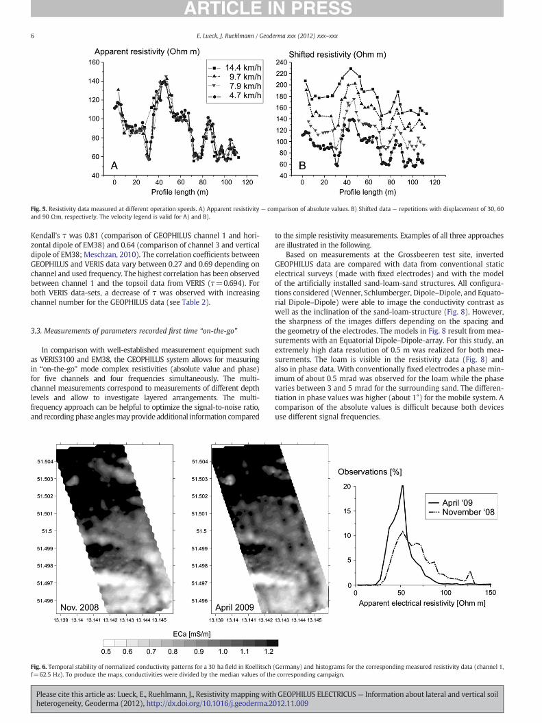
Fig. 5. Resistivity data measured at different operation speeds. A) Apparent resistivity — comparison of absolute values. B) Shifted data — repetitions with displacement of 30, 60and 90 Ωm, respectively. The velocity legend is valid for A) and B).


Kendall's τ was 0.81 (comparison of GEOPHILUS channel 1 and hori-zontal dipole of EM38) and 0.64 (comparison of channel 3 and verticaldipole of EM38; Meschzan, 2010). The correlation coefficients betweenGEOPHILUS and VERIS data vary between 0.27 and 0.69 depending onchannel and used frequency. The highest correlation has been observedbetween channel 1 and the topsoil data from VERIS (τ=0.694). Forboth VERIS data-sets, a decrease of τ was observed with increasingchannel number for the GEOPHILUS data (see Table 2).

3.3. Measurements of parameters recorded first time “on-the-go”

In comparison with well-established measurement equipment suchas VERIS3100 and EM38, the GEOPHILUS system allows for measuringin “on-the-go” mode complex resistivities (absolute value and phase)for five channels and four frequencies simultaneously. The multi-channel measurements correspond to measurements of different depthlevels and allow to investigate layered arrangements. The multi-frequency approach can be helpful to optimize the signal-to-noise ratio,and recordingphase anglesmayprovide additional information compared

Fig. 6. Temporal stability of normalized conductivity patterns for a 30 ha field in Koellitschf=62.5 Hz). To produce the maps, conductivities were divided by the median values of the


to the simple resistivity measurements. Examples of all three approachesare illustrated in the following.

Based on measurements at the Grossbeeren test site, invertedGEOPHILUS data are compared with data from conventional staticelectrical surveys (made with fixed electrodes) and with the modelof the artificially installed sand-loam-sand structures. All configura-tions considered (Wenner, Schlumberger, Dipole–Dipole, and Equato-rial Dipole–Dipole) were able to image the conductivity contrast aswell as the inclination of the sand-loam-structure (Fig. 8). However,the sharpness of the images differs depending on the spacing andthe geometry of the electrodes. The models in Fig. 8 result from mea-surements with an Equatorial Dipole–Dipole-array. For this study, anextremely high data resolution of 0.5 m was realized for both mea-surements. The loam is visible in the resistivity data (Fig. 8) andalso in phase data. With conventionally fixed electrodes a phase min-imum of about 0.5 mrad was observed for the loam while the phasevaries between 3 and 5 mrad for the surrounding sand. The differen-tiation in phase values was higher (about 1°) for the mobile system. Acomparison of the absolute values is difficult because both devicesuse different signal frequencies.

(Germany) and histograms for the corresponding measured resistivity data (channel 1,corresponding campaign.



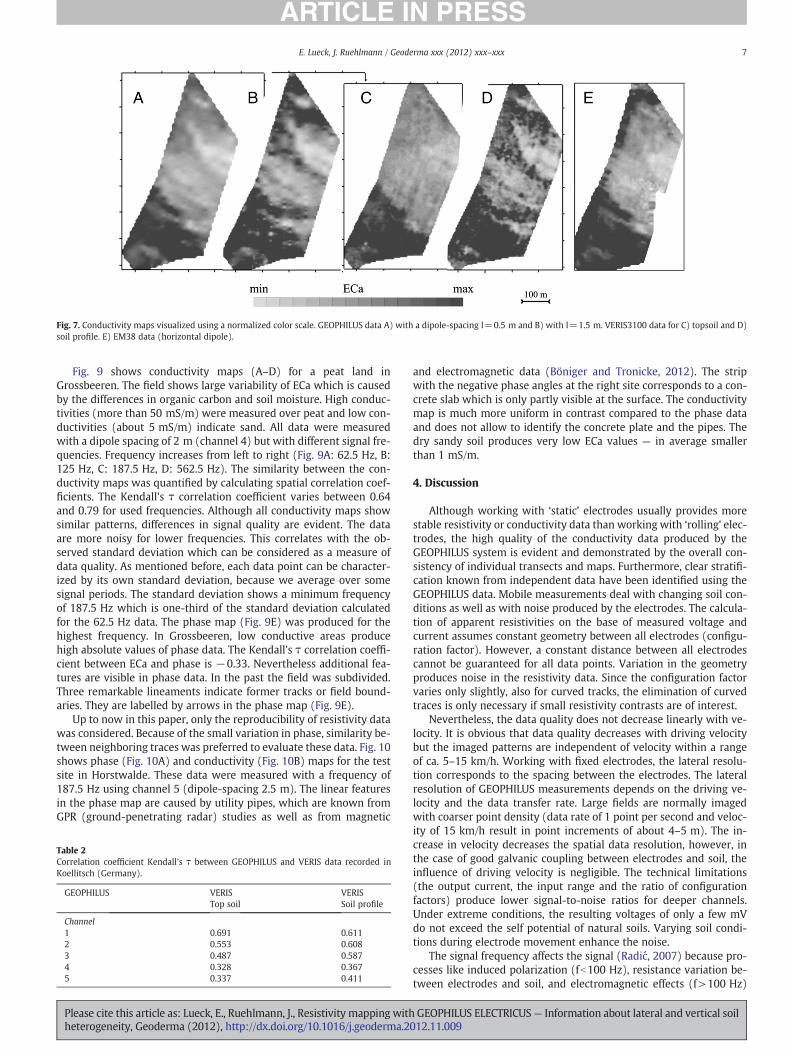
Fig. 7. Conductivity maps visualized using a normalized color scale. GEOPHILUS data A) with a dipole-spacing l=0.5 m and B) with l=1.5 m. VERIS3100 data for C) topsoil and D)soil profile. E) EM38 data (horizontal dipole).


Fig. 9 shows conductivity maps (A–D) for a peat land inGrossbeeren. The field shows large variability of ECa which is causedby the differences in organic carbon and soil moisture. High conduc-tivities (more than 50 mS/m) were measured over peat and low con-ductivities (about 5 mS/m) indicate sand. All data were measuredwith a dipole spacing of 2 m (channel 4) but with different signal fre-quencies. Frequency increases from left to right (Fig. 9A: 62.5 Hz, B:125 Hz, C: 187.5 Hz, D: 562.5 Hz). The similarity between the con-ductivity maps was quantified by calculating spatial correlation coef-ficients. The Kendall's τ correlation coefficient varies between 0.64and 0.79 for used frequencies. Although all conductivity maps showsimilar patterns, differences in signal quality are evident. The dataare more noisy for lower frequencies. This correlates with the ob-served standard deviation which can be considered as a measure ofdata quality. As mentioned before, each data point can be character-ized by its own standard deviation, because we average over somesignal periods. The standard deviation shows a minimum frequencyof 187.5 Hz which is one-third of the standard deviation calculatedfor the 62.5 Hz data. The phase map (Fig. 9E) was produced for thehighest frequency. In Grossbeeren, low conductive areas producehigh absolute values of phase data. The Kendall's τ correlation coeffi-cient between ECa and phase is −0.33. Nevertheless additional fea-tures are visible in phase data. In the past the field was subdivided.Three remarkable lineaments indicate former tracks or field bound-aries. They are labelled by arrows in the phase map (Fig. 9E).

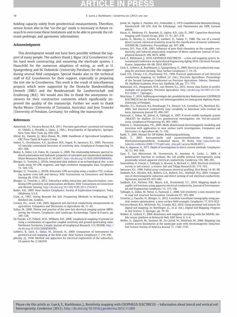
Up to now in this paper, only the reproducibility of resistivity datawas considered. Because of the small variation in phase, similarity be-tween neighboring traces was preferred to evaluate these data. Fig. 10shows phase (Fig. 10A) and conductivity (Fig. 10B) maps for the testsite in Horstwalde. These data were measured with a frequency of187.5 Hz using channel 5 (dipole-spacing 2.5 m). The linear featuresin the phase map are caused by utility pipes, which are known fromGPR (ground-penetrating radar) studies as well as from magnetic

Table 2Correlation coefficient Kendall's τ between GEOPHILUS and VERIS data recorded inKoellitsch (Germany).

GEOPHILUS VERISTop soil

VERISSoil profile

Channel1 0.691 0.6112 0.553 0.6083 0.487 0.5874 0.328 0.3675 0.337 0.411


and electromagnetic data (Böniger and Tronicke, 2012). The stripwith the negative phase angles at the right site corresponds to a con-crete slab which is only partly visible at the surface. The conductivitymap is much more uniform in contrast compared to the phase dataand does not allow to identify the concrete plate and the pipes. Thedry sandy soil produces very low ECa values — in average smallerthan 1 mS/m.

4. Discussion

Although working with ‘static’ electrodes usually provides morestable resistivity or conductivity data than working with ‘rolling’ elec-trodes, the high quality of the conductivity data produced by theGEOPHILUS system is evident and demonstrated by the overall con-sistency of individual transects and maps. Furthermore, clear stratifi-cation known from independent data have been identified using theGEOPHILUS data. Mobile measurements deal with changing soil con-ditions as well as with noise produced by the electrodes. The calcula-tion of apparent resistivities on the base of measured voltage andcurrent assumes constant geometry between all electrodes (configu-ration factor). However, a constant distance between all electrodescannot be guaranteed for all data points. Variation in the geometryproduces noise in the resistivity data. Since the configuration factorvaries only slightly, also for curved tracks, the elimination of curvedtraces is only necessary if small resistivity contrasts are of interest.

Nevertheless, the data quality does not decrease linearly with ve-locity. It is obvious that data quality decreases with driving velocitybut the imaged patterns are independent of velocity within a rangeof ca. 5–15 km/h. Working with fixed electrodes, the lateral resolu-tion corresponds to the spacing between the electrodes. The lateralresolution of GEOPHILUS measurements depends on the driving ve-locity and the data transfer rate. Large fields are normally imagedwith coarser point density (data rate of 1 point per second and veloc-ity of 15 km/h result in point increments of about 4–5 m). The in-crease in velocity decreases the spatial data resolution, however, inthe case of good galvanic coupling between electrodes and soil, theinfluence of driving velocity is negligible. The technical limitations(the output current, the input range and the ratio of configurationfactors) produce lower signal-to-noise ratios for deeper channels.Under extreme conditions, the resulting voltages of only a few mVdo not exceed the self potential of natural soils. Varying soil condi-tions during electrode movement enhance the noise.

The signal frequency affects the signal (Radić, 2007) because pro-cesses like induced polarization (fb100 Hz), resistance variation be-tween electrodes and soil, and electromagnetic effects (f>100 Hz)



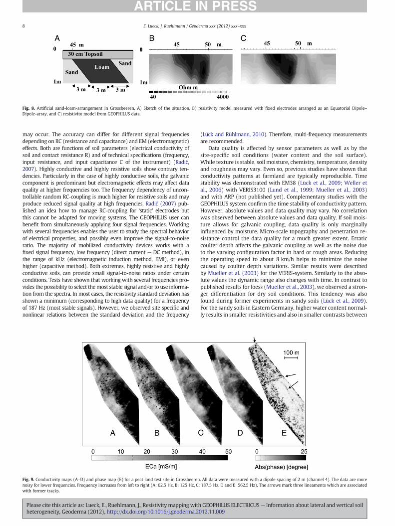
Fig. 8. Artificial sand-loam-arrangement in Grossbeeren. A) Sketch of the situation, B) resistivity model measured with fixed electrodes arranged as an Equatorial Dipole–Dipole-array, and C) resistivity model from GEOPHILUS data.


may occur. The accuracy can differ for different signal frequenciesdepending on RC (resistance and capacitance) and EM (electromagnetic)effects. Both are functions of soil parameters (electrical conductivity ofsoil and contact resistance R) and of technical specifications (frequency,input resistance, and input capacitance C of the instrument) (Radić,2007). Highly conductive and highly resistive soils show contrary ten-dencies. Particularly in the case of highly conductive soils, the galvaniccomponent is predominant but electromagnetic effects may affect dataquality at higher frequencies too. The frequency dependency of uncon-trollable random RC-coupling is much higher for resistive soils and mayproduce reduced signal quality at high frequencies. Radić (2007) pub-lished an idea how to manage RC-coupling for ‘static’ electrodes butthis cannot be adapted for moving systems. The GEOPHILUS user canbenefit from simultaneously applying four signal frequencies. Workingwith several frequencies enables the user to study the spectral behaviorof electrical properties, and possibly even improve the signal-to-noiseratio. The majority of mobilized conductivity devices works with afixed signal frequency, low frequency (direct current — DC method), inthe range of kHz (electromagnetic induction method, EMI), or evenhigher (capacitive method). Both extremes, highly resistive and highlyconductive soils, can provide small signal-to-noise ratios under certainconditions. Tests have shown that working with several frequencies pro-vides the possibility to select themost stable signal and/or to use informa-tion from the spectra. In most cases, the resistivity standard deviation hasshown a minimum (corresponding to high data quality) for a frequencyof 187 Hz (most stable signals). However, we observed site specific andnonlinear relations between the standard deviation and the frequency

Fig. 9. Conductivity maps (A–D) and phase map (E) for a peat land test site in Grossbeerennoisy for lower frequencies. Frequency increases from left to right (A: 62.5 Hz, B: 125 Hz, C:with former tracks.


(Lück and Rühlmann, 2010). Therefore, multi-frequency measurementsare recommended.

Data quality is affected by sensor parameters as well as by thesite-specific soil conditions (water content and the soil surface).While texture is stable, soil moisture, chemistry, temperature, densityand roughness may vary. Even so, previous studies have shown thatconductivity patterns at farmland are typically reproducible. Timestability was demonstrated with EM38 (Lück et al., 2009; Weller etal., 2006) with VERIS3100 (Lund et al., 1999; Mueller et al., 2003)and with ARP (not published yet). Complementary studies with theGEOPHILUS system confirm the time stability of conductivity pattern.However, absolute values and data quality may vary. No correlationwas observed between absolute values and data quality. If soil mois-ture allows for galvanic coupling, data quality is only marginallyinfluenced by moisture. Micro-scale topography and penetration re-sistance control the data quality for a much greater extent. Erraticcoulter depth affects the galvanic coupling as well as the noise dueto the varying configuration factor in hard or rough areas. Reducingthe operating speed to about 8 km/h helps to minimize the noisecaused by coulter depth variations. Similar results were describedby Mueller et al. (2003) for the VERIS-system. Similarly to the abso-lute values the dynamic range also changes with time. In contrast topublished results for loess (Mueller et al., 2003), we observed a stron-ger differentiation for dry soil conditions. This tendency was alsofound during former experiments in sandy soils (Lück et al., 2009).For the sandy soils in Eastern Germany, higher water content normal-ly results in smaller resistivities and also in smaller contrasts between

. All data were measured with a dipole spacing of 2 m (channel 4). The data are more187.5 Hz, D and E: 562.5 Hz). The arrows mark three lineaments which are associated



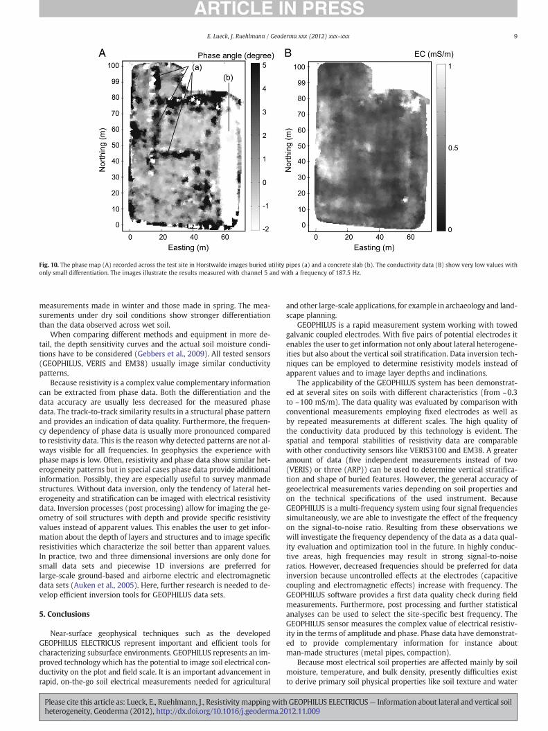
Fig. 10. The phase map (A) recorded across the test site in Horstwalde images buried utility pipes (a) and a concrete slab (b). The conductivity data (B) show very low values withonly small differentiation. The images illustrate the results measured with channel 5 and with a frequency of 187.5 Hz.


measurements made in winter and those made in spring. The mea-surements under dry soil conditions show stronger differentiationthan the data observed across wet soil.

When comparing different methods and equipment in more de-tail, the depth sensitivity curves and the actual soil moisture condi-tions have to be considered (Gebbers et al., 2009). All tested sensors(GEOPHILUS, VERIS and EM38) usually image similar conductivitypatterns.

Because resistivity is a complex value complementary informationcan be extracted from phase data. Both the differentiation and thedata accuracy are usually less decreased for the measured phasedata. The track-to-track similarity results in a structural phase patternand provides an indication of data quality. Furthermore, the frequen-cy dependency of phase data is usually more pronounced comparedto resistivity data. This is the reason why detected patterns are not al-ways visible for all frequencies. In geophysics the experience withphase maps is low. Often, resistivity and phase data show similar het-erogeneity patterns but in special cases phase data provide additionalinformation. Possibly, they are especially useful to survey manmadestructures. Without data inversion, only the tendency of lateral het-erogeneity and stratification can be imaged with electrical resistivitydata. Inversion processes (post processing) allow for imaging the ge-ometry of soil structures with depth and provide specific resistivityvalues instead of apparent values. This enables the user to get infor-mation about the depth of layers and structures and to image specificresistivities which characterize the soil better than apparent values.In practice, two and three dimensional inversions are only done forsmall data sets and piecewise 1D inversions are preferred forlarge-scale ground-based and airborne electric and electromagneticdata sets (Auken et al., 2005). Here, further research is needed to de-velop efficient inversion tools for GEOPHILUS data sets.

5. Conclusions

Near-surface geophysical techniques such as the developedGEOPHILUS ELECTRICUS represent important and efficient tools forcharacterizing subsurface environments. GEOPHILUS represents an im-proved technology which has the potential to image soil electrical con-ductivity on the plot and field scale. It is an important advancement inrapid, on-the-go soil electrical measurements needed for agricultural


and other large-scale applications, for example in archaeology and land-scape planning.

GEOPHILUS is a rapid measurement system working with towedgalvanic coupled electrodes. With five pairs of potential electrodes itenables the user to get information not only about lateral heterogene-ities but also about the vertical soil stratification. Data inversion tech-niques can be employed to determine resistivity models instead ofapparent values and to image layer depths and inclinations.

The applicability of the GEOPHILUS system has been demonstrat-ed at several sites on soils with different characteristics (from ~0.3to ~100 mS/m). The data quality was evaluated by comparison withconventional measurements employing fixed electrodes as well asby repeated measurements at different scales. The high quality ofthe conductivity data produced by this technology is evident. Thespatial and temporal stabilities of resistivity data are comparablewith other conductivity sensors like VERIS3100 and EM38. A greateramount of data (five independent measurements instead of two(VERIS) or three (ARP)) can be used to determine vertical stratifica-tion and shape of buried features. However, the general accuracy ofgeoelectrical measurements varies depending on soil properties andon the technical specifications of the used instrument. BecauseGEOPHILUS is a multi-frequency system using four signal frequenciessimultaneously, we are able to investigate the effect of the frequencyon the signal-to-noise ratio. Resulting from these observations wewill investigate the frequency dependency of the data as a data qual-ity evaluation and optimization tool in the future. In highly conduc-tive areas, high frequencies may result in strong signal-to-noiseratios. However, decreased frequencies should be preferred for datainversion because uncontrolled effects at the electrodes (capacitivecoupling and electromagnetic effects) increase with frequency. TheGEOPHILUS software provides a first data quality check during fieldmeasurements. Furthermore, post processing and further statisticalanalyses can be used to select the site-specific best frequency. TheGEOPHILUS sensor measures the complex value of electrical resistiv-ity in the terms of amplitude and phase. Phase data have demonstrat-ed to provide complementary information for instance aboutman-made structures (metal pipes, compaction).

Because most electrical soil properties are affected mainly by soilmoisture, temperature, and bulk density, presently difficulties existto derive primary soil physical properties like soil texture and water




holding capacity solely from geoelectrical measurements. Therefore,sensor fusion also in the “on-the-go” mode is necessary in future re-search to overcome these limitations and to be able to provide the rel-evant pedologic and agronomic informations.

Acknowledgment

This development would not have been possible without the sup-port of many people. The authors thank J. Bigus (IGZ Grossbeeren) forhis hard work constructing and mounting the electrode system, I.Hauschild for the numerous adaptions of wiring, as well as U.Spangenberg and M. Dubnitzki (University Potsdam) for the supportduring several field campaigns. Special thanks also to the technicalstaff of IGZ Grossbeeren for their support, especially in preparingthe test site in Grossbeeren. This work is the result of miscellaneousprojects which were supported by the Deutsche BundesstiftungUmwelt (DBU) and the Bundesanstalt für Landwirtschaft undErnährung (BLE). We would also like to thank the anonymous re-viewers for their constructive comments which significantly im-proved the quality of the manuscript. Further we want to thankNysha Munro (University of Tasmania, Australia) and Jens Tronicke(University of Potsdam, Germany) for editing the manuscript.

References

Adamchuk, V.I., Viscarra Rossel, R.A., 2011. Precision agriculture: proximal soil sensing.In: Gliński, J., Horabik, J., Lipiec, J. (Eds.), Encyclopedia of Agrophysics. Springer,New York, New York, pp. 650–656.

Allred, B.J., Daniels, J.J., Reza Ehsani, M., 2008. Handbook of Agricultural Geophysics.CRC Press Taylor & Francis Group.

Auken, E., Christiansen, A.V., Jacobsen, B.H., Foged, N., Sørensen, K.I., 2005. Piecewise1D laterally constrained Inversion of resistivity data. Geophysical Prospecting 53,497–506.

Binley, A., Slater, L.D., Fukes, M., Cassiani, G., 2005. The relationship between spectral in-duced polarization and hydraulic properties of saturated and unsaturated sandstone.Water Resources Research 41, W12417. http://dx.doi.org/10.1029/2005WR004202.

Böniger, U., Tronicke, J., 2010a. Integrated data analysis at an archaeological site: a casestudy using 3D GPR, magnetic, and high-resolution topographic data. Geophysics75, 169–176.

Böniger, U., Tronicke, J., 2010b. Kinematic GPR surveying using a modern TTS: evaluat-ing system cross-talk and latency. IEEE Transactions on Geoscience and RemoteSensing 48, 3792–3798.

Böniger, U., Tronicke, J., 2012. Subsurface utility extraction and characterization: com-bining GPR symmetry and polarization attributes. IEEE Transactions on Geoscienceand Remote Sensing. http://dx.doi.org/10.1109/TGRS.2011.2163413.

Butler, D.K., 2005. Near-Surface Geophysics. Society of Exploration Geophysics, Tulsa,Oklahoma, U.S.A.

Clark, A., 1997. Seeing Beneath the Soil. Prospecting Methods in Archaeology. B.T.Batsford Ltd., London.

Corwin, D.L., Lesch, S.M., 2005. Apparent soil electrical conductivity measurements inagriculture. Computers and Electronics in Agriculture 46, 11–43.

Dabas, M., 2009. Theory and practice of the new fast electrical imaging system ARP©.Seeing the Unseen. Geophysics and Landscape Archaeology. Taylor & Francis, pp.105–126.

De Pascale, G.P., Pollard, W.H., Williams, K.K., 2008. Geophysical mapping of ground iceusing a combination of capacitive coupled resistivity and ground-penetrating radar,Northwest Territories, Canada. Journal of Geophysical Research 113, F02S90. http://dx.doi.org/10.1029/2006JF000585.

Gebbers, R., Lück, E., Dabas, M., Domsch, H., 2009. Comparison of instruments forgeoelctrical soil mapping at the field scale. Near Surface Geophysics 7, 179–190.

Jakosky, J.J., 1938. Method and apparatus for electrical exploration of the subsurface.US-patent No. 2.138.818.


Jonek, W., Sigulla, E., Paschen, H.G., Frohmüller, C., 1979. Geoelektrische Messeinrichtung.Patentschrift 145 670, Amt für Erfindungs- und Patentwesen der DDR, Germanpatent.

Kuras, O., Meldrum, P.I., Beamish, D., Ogilvy, R.D., Lala, D., 2007. Capacitive ResistivityImaging with Towed Arrays. JEEG 12 (3), 267–279.

Lavoie, D., Mozley, E., Corwin, R., Lambert, D., Valent, P., 1988. The use of a towed,direct-current, electrical resistivity array for the classification of marine sediments.OCEANS 88. Conference, Proceedings, pp. 397–408.

Lesmes, D.P., Frye, K.M., 2001. Influence of pore fluid chemistry on the complex con-ductivity and induced polarization responses of Berea sandstone. Journal of Geo-physical Research 106, 4079–4090.

Lück, E., Rühlmann, J., 2010. GEOPHILUS ELECTRICUS — a new soil mapping system. In-ternational Conference on Agricultural Engineering AgEng 2010. Clermont Ferrand,France, September 06–08. 2010, REF319.

Lück, E., Gebbers, R., Ruehlmann, J., Spangenberg, U., 2009. Electrical conductivity map-ping for precision farming. Near Surface Geophysics 7, 15–25.

Lund, E.D., Christy, C.D., Drummond, P.E., 1999. Practical applications of soil electricalconductivity mapping. In: Stafford, J.V. (Ed.), Precision Agriculture. Proceedingsof the Second European Conference on Precision Agriculture. Odense, Denmark,99. Sheffield Academic Press Ltd, Sheffield, UK, pp. 771–779.

Mahmood, H.S., Hoogmoed, W.B., van Henten, E.J., 2012. Sensor data fusion to predictmultiple soil properties. Precision Agriculture. http://dx.doi.org/10.1007/s11119-012-9280-7 (Springer).

Meschzan, T., 2010. Auflösungsvermögen des geoelektrischen Bodensensors GEOPHILUSELECTRICUS bei der Erfassung von Inhomogenitäten im Untergrund, diploma thesis.University of Potsdam.

Mueller, T.G., Hartsock, N.J., Stombaugh, T.S., Shearer, S.A., Cornelius, P.L., Barnhisel, R.I.,2003. Soil electrical conductivity map variability in limestone soils overlain byloess. Agronomy Journal 95, 496–507.

Panissod, C., Dabas, M., Jolivat, A., Tabbagh, A., 1997. A novel mobile multipole system(MUCEP) for shallow (0–3 m) geoelectrical investigation: the ‘Vol-de-canards’array. Geophysical Prospecting 45, 983–1002.

Pellerin, L., Wannamaker, P.E., 2005. Multi-dimensional electromagnetic modeling andinversion with application to near surface earth investigations. Computers andElectronics in Agriculture 46, 71–102.

Radić, T., 2005. Manuel for SIP Rabbit. Bedienungsanleitung.Radić, T., 2007. Instrumentelle und auswertemethodische Arbeiten zur

Wechselstromgeoelektrik. Graduated thesis, TU Berlin http://opus.kobv.de/tuberlin/volltexte/2008/1779/pdf/radic_tino.pdf (access 04.08.2011).

Roy, A., Apparao, A., 1971. Depth of investigation in direct current methods. Geophysics36 (5), 943–959.

Saey, T., Van Meirvenne, M., Vermeersch, H., Ameloot, N., Cockx, L., 2009. Apedotransfer function to evaluate the soil profile textural heterogeneity usingproximally sensed apparent electrical conductivity. Geoderma 150, 389–395.

Samouёlian, A., Cousin, I., Tabbagh, A., Bruand, A., Richard, G., 2005. Electrical resistivitysurvey in soil science: a review. Soil and Tillage Research 83, 173–193.

Sørensen, K.I., 1996. Pulled array continuous electrical profiling. First Break 14, 85–90.Sudduth, K.A., Kitchen, N.R., Bollero, G.A., Bullock, D.G., Wiebold, W.J., 2003. Compari-

son of electromagnetic induction and direct sensing of soil electrical conductivity.Agronomy Journal 95, 472–482.

Sudduth, K.A., Kitchen, N.R., Myers, D.B., Drummond, S.T., 2010. Mapping depth toargillic soil horizons using apparent electrical conductivity. Journal of Environmen-tal and Engineering Geophysics 15, 135–146.

Tabbagh, A., Dabas, M., Hesse, A., Panissod, C., 2000. Soil resistivity: a non-invasive toolto map soil structure horizonation. Geoderma 97, 393–404.

Tronicke, J., Paasche, H., Böniger, U., 2012. Crosshole traveltime tomography using par-ticle swarm optimization: a near-surface field example. Geophysics 77, R19–R32.

Viscarra Rossel, R.A., McKenzle, N.J., Grundy, M.J., 2010. Using proximal soil sensors fordigital soil mapping. In: Boettinger, J.L., et al. (Ed.), Digital Soil Mapping, Progressin Soil Science, 2. Springer, pp. 79–92.

Walker, R., Linford, P., 2006. Resistance and magnetic surveying with the MSP40, mo-bile sensor platform at Kelmarsh Hall. ISAP News 9, 3–4.

Weller, U., Zipprich, M., Sommer, M., Zu Castell, W., Wehrhan, M., 2006. Mapping claycontent across boundaries at the landscape scale with electromagnetic induction.Soil Science Society of America Journal 71, 1740–1747.


http://dx.doi.org/10.1029/2005WR004202

http://dx.doi.org/10.1109/TGRS.2011.2163413

http://dx.doi.org/10.1029/2006JF000585

http://dx.doi.org/10.1007/s11119-012-9280-7

http://dx.doi.org/10.1007/s11119-012-9280-7

http://opus.kobv.de/tuberlin/volltexte/2008/1779/pdf/radic_tino.pdf

http://opus.kobv.de/tuberlin/volltexte/2008/1779/pdf/radic_tino.pdf


Documents

Resistivity mapping with GEOPHILUS ELECTRICUS ... · Resistivity mapping with GEOPHILUS ELECTRICUS — Information about lateral and vertical soil heterogeneity E. Lueck a,⁎, J