Engineering Geology 117 (2011) 121–133

Contents lists available at ScienceDirect

Engineering Geology

j ourna l homepage: www.e lsev ie r.com/ locate /enggeo

Electrical resistivity in support of geological mapping along the Panama Canal

Dale F. Rucker a,⁎, Gillian E. Noonan a, William J. Greenwood b

a hydroGEOPHYSICS, Inc. 2302 N Forbes Blvd, Tucson, AZ 85745, USAb Pacific Northwest National Laboratory, 902 Battelle Boulevard, P.O. Box 999, MSIN K9-33, Richland, WA 99352, USA

⁎ Corresponding author. Tel.: +1 520 647 3315.E-mail addresses: druck8240@gmail.com, drucker@h

gnoonan@hgiworld.com (G.E. Noonan), william.greenw(W.J. Greenwood).

0013-7952/$ – see front matter © 2010 Elsevier B.V. Aldoi:10.1016/j.enggeo.2010.10.012

a b s t r a c t

a r t i c l e i n f o

Article history:Received 15 February 2010Received in revised form 7 October 2010Accepted 12 October 2010Available online 19 October 2010

Keywords:GeophysicsPanama CanalResistivityGeological mappingDredging

Dredging and widening of the Panama Canal is currently being conducted to allow larger vessels to transit toand from the Americas, Asia, and Europe. Dredging efficiency relies heavily on knowledge of the types andvolumes of sediments and rocks beneath the waterway to ensure the right equipment is used for theirremoval. To aid this process, a waterborne streaming electrical resistivity survey was conducted along theentire length of the canal to provide information on its geology. Within the confines of the canal, a total of 663line-kilometers of electrical resistivity data were acquired using the dipole–dipole array. The support of thesurvey data for dredging activities was realized by calibrating and qualitatively correlating the resistivity datawith information obtained from nearby logged boreholes and geological maps.The continuity of specific strata was determined in the resistivity sections by evaluating the continuity ofsimilar ranges of resistivity values between boreholes. It was evident that differing geological units andsuccessions can have similar ranges of resistivity values. For example, Quaternary sandy and gravelly alluvialfill from the former river channel of the Chagres River had similar resistivity ranges (generally from 40 to250 Ωm) to those characteristic of late Miocene basalt dikes (from 100 to 400 Ωm), but for quite differentreasons. Similarly, competent marine-based sedimentary rocks of the Caimito Formation were similar inresistivity values (ranging from 0.7 to 10 Ωm) to sandstone conglomerate of the Bohio Formation.Consequently, it would be difficult to use the resistivity data alone to extrapolate more complex geotechnicalparameters, such as the hardness or strength of the substrate. A necessary component for such analysesrequires detailed objective information regarding the specific context from which the geotechnicalparameters were derived. If these data from cored boreholes and detailed geological surveys are taken intoaccount, however, then waterborne streaming resistivity surveying can be a powerful tool. In this case, itprovided inexpensive and highly resolved quantitative information on the potential volume of loosesuctionable material along the Gamboa Sub-reach, which could enable large cost savings to be made on amajor engineering project involving modification of one of the most important navigable waterways in theworld.

giworld.com (D.F. Rucker),ood@pnl.gov

l rights reserved.

© 2010 Elsevier B.V. All rights reserved.

1. Introduction

In October 2006, the Panamanian people voted to expand thePanama Canal. The national referendum was overwhelmingly ap-proved (New York Times, 2006), with construction set to beginshortly after. Using a multi-faceted approach, the expansion proposedto allow larger ships carrying increased cargo loads through the canal.The approach included 1) a new set of lock facilities at both Atlanticand Pacific entrances, 2) an increased water level in Gatun Lake, and3) a deeper and wider navigation channel through Gatun Lake andGaillard Cut (ACP, 2007). Currently, the largest vessel that can betransported through the canal is the Panamax (i.e., a vessel with a

restricted length of 275 m, width of 32 m, and draft of 12 m). Theexpansion would allow post-Panamax ships to have a maximum draftof 15.2 m by, in part, increasing the lake's height by 0.45 m anddredging the navigable channel by 1.2 m.

Dredging of the Panama Canal is expected to take seven years tocomplete, finishing in 2014. The proposed volume of material to beremoved from deepening and widening of the Gatun Lake andGaillard Cut is approximately 23×106 m3, with 17×106 m3 removedfrom Gatun Lake and 6×106 m3 from Gaillard Cut. The ease by whichthis material can be excavated will depend on the specific rock typesencountered along the waterway. The Panama Canal Authority (ACP)currently uses a cutter suction dredge and dipper (or hopper) dredgeto maintain the canal. These dredges would be used to help in theexpansion project. The cutter suction dredge removes loose sedi-ments such as gravels, sands, and silts, as well as some hardened clayand softer, weathered rock. Hard rock must be drilled and blasted,after which the dipper dredge removes the loosened material. Land-

122 D.F. Rucker et al. / Engineering Geology 117 (2011) 121–133

based dredging and widening is also conducted along the canal's edgewith earth-moving equipment.

Knowledge of different rock types along the canal, therefore, iscritical in maintaining a high dredging efficiency. To this end, the ACPmaintains a library of borehole logs that are used to developgeological models of the canal. Most of these are concentrated alongthe Gaillard Cut and in areas of previous expansion. Average boreholeseparation in the Gaillard Cut is approximately 50 m. Within theGatun Lake area, on the other hand, the boreholes are separated onaverage by 450 m, equating to approximately 15×104m3 of dredgematerial between the boreholes. Rock types can change significantlyover this distance, especially along the Gamboa Reach, due to themore recent geological events that have taken place since theOligocene.

Geophysical methods are used to fill data gaps and interpolategeological information in complex marine, lacustrine, and riverineenvironments. For example, (Nordfjord et al., 2009) presented aseismic reflection analysis of the stratigraphy near the New Jerseyshoreline. Similarly, (Osterman et al., 2009) used the seismicreflection method to map the shoreline near Apalachicola Bay, Floridato understand sedimentary processes during the Holocene. Magneticand electromagnetic methods have also proven successful in mappingmarine geological structures as demonstrated by Constable et al.(2009), Faggioni et al. (2003), Bourlon et al. (2002), and Dehler andPotter (2002). These methods are capable of imaging deeply (100 s ofmeters to kilometers) and providing additional information useful forgeological models beyond that which could be obtained throughconventional drilling alone.

Rarely is the electrical resistivity geophysical method used to maplithologies underlying waterways, especially in support of engineer-ing construction projects. Typically, the resistivity method is used inwaters to understand the location and quality of submarinegroundwater discharge (see Swarzenski et al., 2006, 2007; Kroeger

Fig. 1. Location of the Panama Canal within central Panama. The route of the canal is maridentifies major tectonic features of the broader region (adapted from Coates et al., 2004).

et al., 2007; Taniguchi et al., 2007, 2008) or near coastlines to track saltwater intrusion into nearby aquifers (Comte and Banton, 2007; deFranco et al., 2009; Hayley et al., 2009; Martinez et al., 2009).Resistivity can provide an indication of relative degrees of saturationand porosity of the rock. This is not generally possible for otherwaterborne geophysical methods such as seismic reflection andground penetrating radar.

We present a study of an electrical resistivity survey that has beenacquired in the Panama Canal. The survey was conducted to supportthe ongoing dredging project and to assess the lithological variationsacross the parts of the canal that are being widened and deepened.Electrical resistivity was chosen for the Panama Canal mappingproject due to its low expense, low susceptibility to environmentaland construction noise, and fast turn-around of information relative toother more likely geophysical candidates such as seismic refraction.Data acquisition covered the entire 50 km navigable waterway fromthe Gatun Locks in the north to the Pedro Miguel Locks in the south(route A–Q in Fig. 1), with parallel surveyed lines spaced 25 m apartacross the open channel. The resistivity data collected were of highdensity and good quality, enabling detailed geological interpretationsof contacts, stratigraphy, and structure.

2. Setting

The Panama Canal is a man-made shipping waterway thatconnects the Caribbean Sea to the Gulf of Panama across the Isthmusof Panama (Fig. 1). The canal links the Atlantic and Pacific oceansusing a set of artificial lakes, a long overland cut channel, and threesets of locks. The width of the navigable waterway is narrow in someareas and the expansion will ease these restrictions to allow thepassage of larger ships by widening the entire length of the navigablewaterway. Up to 14,000 transits are made through the canal each yearand each transit takes approximately 24 h to complete (Llacer, 2005).

ked with a solid line with specific turns identified for surveying reference. Inset map

Table 1Names and locations of markers along the Panama Canal.

Reach Sub-reach Turn Location of turn on Fig. 1 Positiona

Gatun Lake Third Locks Gatun A 12 K+627Gatun Lake Third Locks Trinidad B 18 K+582Gatun Lake Pena Blanca Pena Blanca C 25 K+749Gatun Lake Bohio Bohio D 28 K+288Gatun Lake Buena Vista Frijoles E 32 K+821Gatun Lake Tabernilla Tabernilla F 37 K+346Gamboa San Pablo Caimito G 41 K+456Gamboa San Pablo Mamei H 43 K+129Gamboa Gamboa Juan Grande I 44 K+046Gamboa Gamboa Santa Cruz J 49 K+143Gamboa Chagres Bas Obispo K 50 K+599Gaillard Cut Bas Obispo Las Cascadas L 53 K+675Gaillard Cut Cascade Cunette M 55 K+374Gaillard Cut Cunette Lirio N 57 K+575Gaillard Cut Culebra Culebra O 60 K+097Gaillard Cut Cucaracha Cartagena P 61 K+958Gaillard Cut Paraiso Paraiso Q 63 K+430

a Kilometers and meters from canal starting location in Atlantic Ocean.

123D.F. Rucker et al. / Engineering Geology 117 (2011) 121–133

The Panama Canal watershed and the man-made Gatun Lake wereimportant water sources during the canal's construction and use. Thelake was formedwhen the Chagres River was dammed in 1910 (Kellerand Stallard, 1994). The lake was filled by 1914, and served as themain waterway of the canal. It has also served as a major freshwaterbarrier to the dispersal of biota between the two oceans (Aron andSmith, 1971). The Gatun Lake covers an area of 436 km2 at 26.7 mabove sea level with a mean water storage capacity of 776×106m3.The water levels are controlled in the lake to within 2 m/yr by theMadden Dam on the upper Chagres River and the Gatun Dam at thelower Chagres (Zaret, 1984). Other lakes include the Alhajuela Lake,which covers an area of 50.2 km2 at 76.8 m above sea level and theMiraflores Lake that covers an area of 3.94 km2 at 16.5 m above sealevel.

The Gaillard Cut portion of the canal is about 13 km and connectsthe Gatun Lake to the Miraflores Lake. The original width of the cutwas about 92 m andwaswidened between 1930 to 1970 tomore than150 m. The current expansion project will ensure the minimumwidthis 280 m along straight portions and 320 m in curves. Maintenanceand dredging of the canal has been continuously conducted during thelife of the canal to ensure that debris is removed from the waterway.

For the purpose of discussion in this paper, the canal has beendivided into three main reaches: the Gatun Lake Reach, the GamboaReach, and the Gaillard Cut Reach. Each reach is then divided into Sub-reaches that extend between 2 and 7 km in length; there are 14 totalSub-reaches. The transition between adjacent Sub-reaches is markedby a turn, which represents a physical turn that a vessel makes as ittransits the canal. The turns have set positions that correspond to thedistance from a starting point located in the Atlantic Ocean, just off the

Table 2Geological formations within the Panama Canal basin.

Stratigraphical name Rock type

Unconsolidated sediments Sands, silts, gravelsUnconsolidated sediments Organically rich sands and siltsChagres Fm. Massive, generally fine-grained sandstonePedro Miguel Fm. Basalt and agglomerateCucaracha Fm. Claystone, sandstone, conglomerate, and ligniteGatun Fm. Marine sandstone, siltstone, and conglomerateCulebra Fm. Marine mudstone, sandstone, limestone, and conglomCaimito Fm. Tuffaceous sandstone, tuffaceous siltstone, conglomer

agglomerate, and limestoneLas Cascadas Fm. Agglomeratic tuffBohio Fm. Siltstone, sandstone, and conglomerateBas Obispo Fm. TuffGatuncillo Fm. Marine mudstone, siltstone, and limestone

coast from the city of Colon. Table 1 lists the details of the Reaches,Sub-reaches, and turns through the canal. The positions can be used tohelp interpret the location of geological descriptions relative to theelectrical resistivity survey data.

3. Geology

The Isthmus of Panama is in the region of four main tectonic platesof South America, Nazca, Cocos, and Caribbean (inset map of Fig. 1),and has been referred to as the Panama block (Adamek et al., 1988;Silver et al., 1990) or Panama microplate (Fisher et al., 1994; Coateset al., 2004). The Isthmus is part of a volcanic arc formed in earlyMiocene around 17 Ma (Coates et al., 2003; Coates et al., 2004;Molnar, 2008) in response to the subduction of the Cocos and Nazcaplates under the Caribbean plate and Panama block at the MiddleAmerica Trench (Morell et al., 2008). The collision is thought to haveproduced the distinctive shape of the isthmus (Mann and Corrigan,1990; Silver et al., 1990).

The Panama Canal Basin is structurally complex (Kirby et al., 2008)owing to the presence of a regional shear zone trending northwest–southeast, which is aligned almost nearly parallel to the Panama Canal(Case, 1974). Numerous northeast–southwest trending faults are alsopresent (Pratt et al., 2003). As described by Jones (1950), the faults aretypically high angle (N60°) and include normal, reverse, and strike-slip (Lowrie et al., 1982) with a wide range of offsets (cm to km scale).Major faults within the Gatun Lake Reach and Gaillard Cut Reach havebeen documented in the most recent geological map of the areaproduced by Stewart et al. (1980). Other structural maps includethose of Jones (1950) and Lowrie et al. (1982).

Bedrock in the Gatun Lake area comprises Cretaceous basaltic andandesitic lavas, which originated as submarine volcanic rock. Theseform the ‘basement’ sequence. They were strongly deformed, possiblyprior to the early Eocene, and were intruded by dioritic and daciticrocks (Woodring, 1957). Eocene to late Miocene intrusive, volcanic,and sedimentary rocks underlie portions of the canal (Jones, 1950),and are important in the context of the present study. The lowermostEocene Gatuncillo Formation unconformably overlies the basementvolcanic rocks. It contains a number of sequences of marinemudstone,siltstone, and limestone. The lithology crops out in the east portion ofthe canal basin near the Alhajuela Lake area.

Oligocene units include the Bohio Formation, which containssiltstone, sandstone, and conglomerate, and the Bas Obispo Forma-tion, which mainly comprises volcanic tuff. Both formations aremapped near Gamboa Reach and in the upper Gaillard Cut Reach. TheBas Obispo Formation generally grades northward into the BohioFormation (Woodring 1957). The Las Cascadas Formation is also ofOligocene age and consists of agglomeratic tuff, but is primarilyrestricted to the Gaillard Cut Reach. Table 2 lists the units, age, andcomposition of the major units of the basin.

Age Distribution

Holocene GamboaHolocene Gatun LakeLate Miocene / Pliocene Gatun LakeLate Miocene Gaillard CutMiocene Gaillard CutEarly Miocene Gatun Lake

erate Early Miocene Gaillard Cutate, tuff, Late Oligocene Gatun Lake, Gamboa

Late Oligocene Gaillard CutEarly Oligocene Gatun Lake, GamboaEarly Oligocene Gamboa, Gaillard CutEocene Gatun Lake, Gamboa, Gaillard Cut

124 D.F. Rucker et al. / Engineering Geology 117 (2011) 121–133

The stratigraphic record for the Miocene marine sedimentaryrocks within the Gaillard Cut Reach has undergone several revisions.The following account of the Miocene sequence is principally takenfrom Kirby et al. (2008) and Johnson and Kirby (2006). The CulebraFormation of early Miocene age, which overlies the Oligocene LasCascadas Formation, is composed of marine mudstone, sandstone,limestone, and conglomerate. Johnson and Kirby (2006) describe ninefacies within the Culebra, five of which belong to the Emperadorlimestone; this limestone is interstratified between mudstone aboveand sandstone below. The middle Miocene Cucaracha Formationabove the Culebra Formation contains claystone, sandstone, con-glomerate, and lignite, each with some degree of paleosol develop-ment (Retallack and Kirby, 2007). The PedroMiguel Formation, whichcomprises basalt and agglomerate, overlies the Cucaracha Formation.

The following formations occur in ascending order in the Gamboaand Gatun Lake Reaches: Bohio (early Oligocene); Caimito (lateOligocene); Gatun (early Miocene); and Chagres (late Miocene / earlyPliocene). Each formation contains a few marine fossils, althoughthese are less evident in the Bohio Formation. The Caimito Formationconsists of tuffaceous sandstone, tuffaceous siltstone, conglomerate,tuff, agglomerate, and limestone (Woodring, 1957). The GatunFormation contains marine sandstone, siltstone, and conglomerate.The Chagres Formation is a sandstone that has a thin outcrop alongthe Caribbean corridor.

Unconsolidated sediments, ranging from Pleistocene to recent inage overlie the Miocene strata across the study area. Toward thenorthwestern side of the canal basin, near the Caribbean coast, thedeposits comprise a black organic-mixed ‘Muck’. Much of thismaterial was laid down in swamps and consists of a mixture of silt,very fine-grained organic debris, and partly carbonized wood, stems,

Fig. 2. Geology of the Gatun Lake Reach (turns A–F), showing the canal boundary, resistivity lirepresents sand-dominated unconsolidated deposits, Qa (c) represents clay-dominated uinformation in Kirby et al. (2008) and Retallack and Kirby (2007).

and leaves (Woodring, 1957). Further southeast, towards the GamboaReach and the former mouth of the Chagres River, particularly wherethe navigable route of the canal across the Gatun Lake intersects theformer meandering course of the river, the sediments are more likelyto be cleaner and of fluvial origin. Gravels and coarse sands can befound in the upper sedimentary record.

Figs. 2 to 4 show the geology of the Panama Canal Basin. Fig. 2focuses on the Gatun Lake Reach and turns A–F. The northern portionof the canal is dominated by a younger strata, primarily comprisingthe Gatun Formation and Quaternary deposits. To the south and east,the age of the rocks increases to range from late Oligocene to earlyOligocene. The late Oligocene is represented by the CaimitoFormation; the early Oligocene is represented by the Bohio Formation.Late Miocene basaltic intrusions are sporadically developed through-out the area. The lower portion of Fig. 2 shows logged data from agroup of selected boreholes. The geological data are presented as theywere recorded in the mid 1940 s, and the water depth has changedsignificantly in several areas since the borings were made. Severallocations along the canal are characterized by particularly deepdeposits of unconsolidated material. On Fig. 2, these have beendesignated as either being sand/silt-dominated (s) or clay-dominated(c) with a subscript by the rock designation. The particulardesignations will be important later when comparing the geologicallogs to the geophysical data. The difference between weathered and‘hard’ rock is also denoted by a hatching for the former.

Fig. 3 shows the Gamboa Reach segment of the canal from turns F–K. The rocks are generally older than those along the Gatun Reach. Thecanal itself appears to straddle the boundaries between severaldifferent rock types, typically with sedimentary rocks on one side andvolcanic rocks on the other. Knowing the exact transition between the

nes, and borehole locations. Geological logs are also shown for a several boreholes. Qa(s)nconsolidated deposits. Figure adapted from Stewart et al. (1980) and modified per

Fig. 3. Geology of the Gamboa Reach (turns F–K), showing the canal boundary, resistivity lines, and borehole locations. Geological logs are also shown for several boreholes. Figureadapted from Stewart et al. (1980) and modified per information in Kirby et al. (2008) and Retallack and Kirby (2007).

Fig. 4. Geology of the Gaillard Cut Reach (turns K–Q), showing the canal boundary, resistivity lines, and borehole locations. Geological logs are also shown for several boreholes.Figure adapted from Stewart et al. (1980) and modified per information in Kirby et al. (2008) and Retallack and Kirby (2007).

125D.F. Rucker et al. / Engineering Geology 117 (2011) 121–133

126 D.F. Rucker et al. / Engineering Geology 117 (2011) 121–133

different rock types would probably facilitate a better dredgingschedule and cost, particularly as the rocks of the Bohio Formation aretypically harder than those of the Caimito Formation. The easternmostboreholes show a transition from sedimentary rocks of the BohioFormation to tuff, which is characteristic of the Bas Obispo Formation.Fig. 4 shows the Gaillard Cut Reach as it generally transitions fromolder strata in the north (e.g., the Las Cascadas Formation) to youngerstrata in the south (e.g., the Pedro Miguel Formation). This representsa general transition from Oligocene tuffs of the Bas Obispo Formationand porphyry of the Caraba Formation into Miocene andesite andagglomerate overlain by marine sedimentary rocks. The figure,originally taken from Stewart et al. (1980), has been modified perdiscussions in Kirby et al. (2008) and Retallack and Kirby (2007),whereby the original La Boca Formation of Stewart et al. (1980) wassuggested to actually be a lower member of the Culebra Formation.Numerous minor faults are observed perpendicular to the canal.

Given the low density of borehole information in the Gatun Reachand high degree of lateral variation in the rock types that crop out inthe Gamboa Reach, it was envisioned that electrical resistivityimaging of subcanal sediments would help expand the geologicalknowledge of the area as well as provide useful information for canalexpansion. It was expected that different rock types would havesufficient variability in resistivity values to enable the mapping ofhidden contacts. Unfortunately, it is difficult to predict beforehand areasonable resistivity value for each lithology, owing to variedsubsurface conditions such as the porosity, dissolution of host-rockmaterial, competency, and other factors. The borehole data providedan important means, therefore, by which the resistivity data could becalibrated. The remaining sections describe the acquisition, data, andinterpretation of the resistivity images acquired from Gatun to thePedro Miguel Locks.

4. Methodology

Resistivity is a volumetric property that describes the resistance ofelectrical current flow within a medium (Telford et al., 1990; Ruckerand Fink, 2007). Direct electrical current is propagated in rocks andminerals by electronic or electrolytic means. Electronic conductionoccurs in minerals where free electrons are available. Electrolyticconduction, on the other hand, relies on the dissociation of ionicspecies within a pore space. With electrolytic conduction, themovement of electrons varies with the mobility, concentration, andthe degree of dissociation of the ions. Electrolytic conduction isrelatively slow with respect to electronic conduction, due to its masstransfer rate-limiting processes and it is strongly influenced by thestructure of the conducting medium. Competent rock with lowporosity and lowwater saturation generally has high resistivities. Thismakes direct current transmission difficult and the measured voltagegradient high. Weathered rock and loose fill material, on the otherhand, should have lower resistivities, depending on the ionicconstituents and their concentrations.

The resistivity method uses electric current (I) that is injected intothe earth through one pair of electrodes (transmitting dipole) andmeasures the resultant voltage potential (V) across another pair ofelectrodes (receiving dipole). Numerous electrodes can be deployedalong a transect (which may be anywhere from meters to kilometersin length), andmodern equipment is used to automatically switch thetransmitting and receiving electrode pairs through a single multi-corecable connection. Rucker (2010) and Rucker et al. (2009) describe themethodology for land-based surveys, which essentially employs astationary array for acquisition until all readings are made. A marine-based acquisition uses a streaming methodology (Song and Cho,2009). Here, a shorter cable and limited number of electrodes aretowed behind a boat, and the cable is connected to the resistivitymeter on the boat deck. In our study, we used the SuperSting R8(Advanced Geosciences, Inc.), which allowed up to 8 receiving dipoles

to be recorded simultaneously with subsequent measurementsoccurring within seconds. The electrode arrangement is such thatthe closest set of electrodes behind the boat is the transmitting dipoleand the remainders are the receiving dipoles. In addition to theresistivity set up, ancillary measurements were made such as positionusing a real-time differential GPS, bathymetry using an echo sounder,and water temperature and conductivity using a hand-held probe.

Fig. 5a shows a schematic of the towed resistivity cable and thearrangement of electrodes behind the boat. For the Panama Canalsurvey, the design criteria for imaging was a minimum of 8 m belowthe bottom of the canal given a water depth of 15 m. To accommo-date the required depth of investigation, the electrode separation was15 m along the cable; the total cable length was 170 m. In customarynotation, the positions of the voltage dipoles are described as “n”distances away from the transmission dipole. Depth of investigation,then, is a function of n. Simulated plot points of increasing depth aredrawn over the geological section in Fig. 5a to demonstrate how aprofile of the subsurface is measured. The points are only a conventionfor easy viewing of data before full processing occurs. During thisstudy the boat moved along the canal at 4 km/h, and data werecollected approximately every 3.6 s. At this resolution, a sample wascollected every 3.75 m, sufficient to distinguish contacts between rocktypes.

The second design criteria of the survey was to image across thewidth of the canal by acquiring parallel lines spaced 25 m apart. Thedata were acquired by swathing back and forth between the pre-designated turning points (see Fig. 1) and the GPS was used to ensurea sufficient coverage by plotting positional information on a heads-updisplay. In some areas, the canal was up to 320 m wide; up to 14 lineswere acquired to cover these regions. In total, end-to-end resistivitycoverage of the canal was 663 line-kilometers. The differential GPSwas also used to geo-reference all of the data for final processing.

Fig. 5b shows actual measured results for a short section of dataalong the Gamboa Sub-reach (located within the Gamboa Reach). Thedata are presented as voltage normalized to injected current (ortransfer resistance, in ohms) versus towed distance along the canal.The first six dipoles of data are shown; the furthest dipoles of n=7and n=8 were generally too noisy to process. The closest dipolereading (n=1) showed a relatively flat reading of 0.29 ohms acrossthe section. For a homogeneous earth, the resistance (R) can beconverted to resistivity (ρ) using a simple geometric factor, K:

ρ = R•K ð1Þ

and

K = π•n• n + 1ð Þ• n + 2ð Þ•a ð2Þ

where a was the dipole separation (15 m in our arrangement). For aspacing of n=1, the resistivity of the water was 82 Ωm, which wassimilar to that measured by the hand-held conductivity probe (seevalues for lines JP-17 and M-9 in Table 3). The water conductivity wasrelatively low due to the humic nature of the jungle soils and low ionicstrength. For the remaining dipole measurements, the data were nothomogeneous and the underlying sediments were definitely affectingthe value of the resistance as it moved past various rock types. Forexample, the resistance (and hence resistivity) increases dramaticallyaround 800 m, which could have been due to a contact between tworock types. Fig. 5a shows an example of the type of subbottom contactthat could cause the shift in resistance values seen in Fig. 5b.

Since the resistance data for dipoles spacings from n=2…6 werenot measured in a homogenous earth, the applications of equations 1and 2 to individual measurements created an “apparent resistivity.”Automated inverse methods applied through numerical models wereused to convert the apparent resistivity to an estimate of the trueresistivity. The inverse method relied on nonlinear optimization,

Fig. 5. a) Schematic of streaming resistivity acquisition along the Panama Canal with towed cable behind a moving boat. b) Measured transfer resistance for the first six voltagemeasurement pairs. Data were acquired within the Gamboa Sub-reach.

127D.F. Rucker et al. / Engineering Geology 117 (2011) 121–133

requiring an iterative procedure to march towards a solution. Itsobjective is to minimize the difference between the modeled andmeasured apparent resistivity, usually in a weighted least squaressense. The objective function has been updated many times over theyears to also include other terms, such as smooth model constraints(i.e., a smooth model based on minimizing the second spatial deri-vative of the resistivity). The smooth model constraint was invokedfor the inverse models completed on the Panama Canal resistivitydata, similar to the analysis by Henderson et al. (2010) and Passaro(2010). Although, it is recognized that others (e.g., Nassir et al., 2000)have used the robust constraint for modeling salt-water intrusionwith success.

Ancillary data are necessary to ensure as much known informationas possible is entered into the inversion processing routine during theforward calculation step. Critical data include bathymetry and waterresistivity, which describe the properties of the water column abovethe canal bed. By providing this information to the forward modelcode, the inverse estimation procedure to obtain resistivity is onlyperformed on the rock below the water body, thus allowing a moreaccurate depiction of the rock's electrical properties. In general, thewater depth varied from about 12 m to 30 m along the course of thecanal and the water resistivity decreased from 90 Ωm in Gatun Laketo 80Ωm along the Gamboa Reach, gradually decreasing to 55 Ωm at

Table 3Input and output statistics for the resistivity modeling.

Line name Input canal water resistivity from hand-heldconductivity probe (Ω m)

Minimum moresistivity (Ω

G-15 91 2.0PB-13 90 2.6BH-17 93 7.7BV-9 92 3.7TI-4 91 6.1JP-17 87 5.1M-9 83 1.4JG-6 74 8.6GW-5 74 3.6CH-7 68 3.4BO-6 70 2.7C-6 70 2.2CE-7 67 2.4CU-2 67 1.8CC-3 56 2.0PA-4 59 4.5

the southern Pedro Miguel locks (Table 3). The lower resistivity of thewater body within the Gaillard Cut (typically 55 to 75 Ωm) could bedue to increased dissolved solids from runoff along exposed rockbanks.

The code used to inverse model the dataset, RES2DINV (GeotomoSoftware, Malaysia), also required input parameters to effectivelyconstrain the inversion and calculate a unique solution. These inputparameters included stopping criteria (such as a maximumnumber ofiterations=7; convergence limit between measured and modeledapparent resistivity=3%; minimum change in convergence betweensuccessive iterations=0.5%), forward modeling parameters (finiteelement method, number of nodes between adjacent electrodes=4;telescoping layering of 1.04 times the preceding layer) and inverseparameters (starting model equal to the average apparent resistivity;upper and lower resistivity limit of 50 and 0.02 times the startingresistivity value; incomplete Gauss–Newton as described by Loke andDahlin (2002); minimize variation in the resistivity of the waterlayer). In most cases, the default settings were used.

5. Results

An estimate of the true spatial distribution of electrical resistivitywas obtained through inverse modeling using RES2DINV. The aim of

deledm)

Mean modeledresistivity (Ωm)

Maximum modeledresistivity (Ωm)

Model RMS(%)

9.3 84.6 1.1218.2 98.7 1.3321.9 87.7 1.3923.6 89.4 1.1362.8 80.2 1.6620.5 112.2 1.710.1 42.9 1.4540.7 117.5 0.9817.6 137.3 1.4419.6 125.7 1.6614.3 132.3 1.746.2 59.1 2.77

21.4 134.5 1.166.8 92.0 2.56

20.0 625.9 1.4820.1 110.9 1.22

128 D.F. Rucker et al. / Engineering Geology 117 (2011) 121–133

the inversion procedure applied to the data was to obtain a low rootmean square (RMS) error value. The RMS describes the quality of fitbetween modeled and measured apparent resistivity. The desiredRMS is typically on the order of the expected measurement noise inthe apparent resistivity values. To assess this measurement noise forthe Panama Canal data, the transfer resistance data were firstconvolved with a low-pass sinc filter, which has an impulse responseof a sinc function (i.e., sin(x)/x) in the time domain and a rectangularfunction in the frequency domain. The sinc filter removes shortwavelength information that is typical of noise. To filter the data, eachn spacing was filtered separately and the length of the filter was nineadjacent values or 33.75 m long. Fig. 6a shows an example of raw dataacquired from the Cascade Sub-reach (line C-6) for spacings of n=1to 7. Most of the values for the spacing of n=8 were negative andtherefore not used for the analysis. A call-out in the upper right handcorner of Fig. 6a shows the filtering results for a small section alongspacing of n=5. The filtered data were then compared to the originaldata using a simple percent difference; this percent difference wasused as an estimate of the measurement noise and was necessarysince other standard error measures were not available, including arepeat error (an error measurement from stacking repeated measure-

Fig. 6. Assessment of measurement error for resistivity data collected along the Panama Caseparations of n=1 to 7. Inset in upper right corner shows an example of a low pass filtedifference in filtered and raw data, with error plotted versus distance along the line for n=1distance. e) Measurement error for n=7 versus distance.

ments acquired for identical transmitter and receiver pairs) andreciprocal error (an error measurement based on swapping thetransmitter and receiver electrode pair). Fig. 6b to e shows thecalculated percent difference for spacings of n=1, 3, 5, and 7 as afunction of distance along the line. These figures show that as the nspacing increases, the percent difference between raw and filtereddata also increases. Up to a spacing of n=6 (not shown), the increasein the error was marginal, with a standard deviation of 2.6%. At aspacing of n=7 (Fig. 6e), however, the error was significant and wasdeemed too noisy for further inclusion in processing. The large noisewas likely the result of the measurements being lower than thethreshold of the equipment. In general, the quality of the data frommost lines was high with the measured error falling below 2%. Themeasurement error was then used to assess the completion of theinverse modeling, with the final RMS of less than 2% within fiveiterations for most lines. For line C-6, the final RMS of 2.77% wasdeemed sufficient.

The results of the inverse modeling are presented as a profile ofresistivity along the course traversed by the boat. At least one linefrom each of the 14 Sub-reaches is presented in Figs. 7 to 10, whichalso show the location of the turns (A–Q) from Figs. 2 to 4. Fig. 7

nal. a) Raw transfer resistance data along the Cascade Sub-reach (line C-6) for dipoler applied to a portion of the data. b) Measurement error as calculated by the percent. c) Measurement error for n=3 versus distance. d) Measurement error for n=5 versus

Fig. 7. Results of electrical resistivity for the Gatun Lake Reach (turns A–F), shown as contoured profiles for select lines with an exaggeration of 50:1. Locations of individual lines areshown in Fig. 2.

Fig. 8. Enhanced view of resistivity results from subsections within Fig. 7 at anexaggeration of 12.5:1

129D.F. Rucker et al. / Engineering Geology 117 (2011) 121–133

focuses on data acquired within the Gatun Lake Reach and the exactlocations of the lines are shown on Fig. 2. The resistivity profiles aregreatly exaggerated at a scale of 50:1 to help show relevant changes inthe vertical direction; lateral changes typically occur on a muchbroader scale. Fig. 8 focuses on four shorter sub-sections from datawithin Fig. 7 at a less exaggerated scale of 12.5:1. The range ofresistivity values within these sections vary by a factor of 50, from alow of 2 Ωm to a high near 100 Ωm. Table 3 lists the mean and rangesof resistivity values for each line. Interpretations of the resistivity dataare typically made by describing targets of either high or lowresistivity relative to the mean. For the first Sub-reach of the ThirdLocks, line G-15 shows resistivity mostly on the lower end of the scaleexcept for a stretch from 2700 to 4300 m and a few pockets of near-surface higher resistivity values. The borehole logs from Fig. 2 aresuperimposed on top of the contoured resistivity values to help in theinterpretation. The logs show that within the top 34 m this Sub-reachis predominately alluvial fill and Atlantic ‘Muck’ with a few areasunderlain by the Gatun Formation. The resistivity data show a widerange of variability in resistivity for the fill, which could be explainedby an increased volume of either clay or sandy silt sediment. Ingeneral, clay minerals have lower resistivity than sand due to higherelectrical conduction along individual grains in direct contact witheach other (Shevnin et al., 2007). The stretches showing higherresistivity, therefore, are likely dominated by more sandy sequences.Another consideration is that the water in Gatun Lake is relativelyresistive at 90 Ωm. The pore space of the nearer surface sands is filledwith this water making these types of unconsolidated deposits moreprominently resistive with electrical imaging. However, the deepestportions of the sandy material become more conductive with depth.This is likely to indicate either a significant increase in conductive clayor a change in ionic constituents of the pore water. The mean sea levelis plotted (−26.7 m) to demonstrate the possibility that the deepwater becomes brackish from salt water intrusion, thus changing the

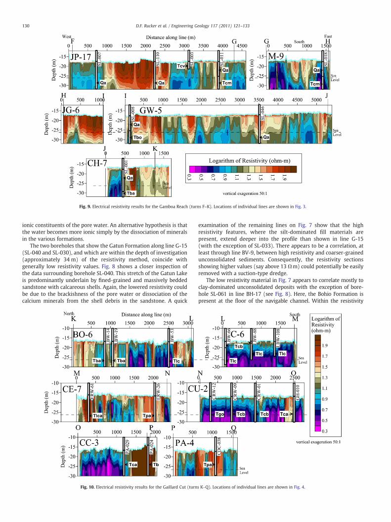
Fig. 9. Electrical resistivity results for the Gamboa Reach (turns F–K). Locations of individual lines are shown in Fig. 3.

130 D.F. Rucker et al. / Engineering Geology 117 (2011) 121–133

ionic constituents of the pore water. An alternative hypothesis is thatthe water becomes more ionic simply by the dissociation of mineralsin the various formations.

The two boreholes that show the Gatun Formation along line G-15(SL-040 and SL-030), and which are within the depth of investigation(approximately 34 m) of the resistivity method, coincide withgenerally low resistivity values. Fig. 8 shows a closer inspection ofthe data surrounding borehole SL-040. This stretch of the Gatun Lakeis predominantly underlain by fined-grained and massively beddedsandstone with calcareous shells. Again, the lowered resistivity couldbe due to the brackishness of the pore water or dissociation of thecalcium minerals from the shell debris in the sandstone. A quick

Fig. 10. Electrical resistivity results for the Gaillard Cut (turn

examination of the remaining lines on Fig. 7 show that the highresistivity features, where the silt-dominated fill materials arepresent, extend deeper into the profile than shown in line G-15(with the exception of SL-033). There appears to be a correlation, atleast through line BV-9, between high resistivity and coarser-grainedunconsolidated sediments. Consequently, the resistivity sectionsshowing higher values (say above 13 Ωm) could potentially be easilyremoved with a suction-type dredge.

The low resistivity material in Fig. 7 appears to correlate mostly toclay-dominated unconsolidated deposits with the exception of bore-hole SL-061 in line BH-17 (see Fig. 8). Here, the Bohio Formation ispresent at the floor of the navigable channel. Within the resistivity

s K–Q). Locations of individual lines are shown in Fig. 4.

131D.F. Rucker et al. / Engineering Geology 117 (2011) 121–133

record at SL-061, the values are lower than the average and can betracked laterally for about 400 m. If the low resistivity can be directlyattributed to the Bohio Formation, then it is likely that this rock,consisting primarily of coarse-grained sandstone and interbeddedconglomerate with pebbles altered to dark clayey minerals, alsoextends from station 400 m to station 1000 m along the line. The lowresistivity could be a result of the dissociation of altered clayminerals inthe porewater and low diffusion of resistive lake water. Another featurethat prominently appears in line T1-4 around station 4000 m is thesteeply bounded, narrow zone of high resistivities that extend to depth(see Fig. 8). The geological map indicates massive basaltic intrusionshere and the zone could represent this type of material. If this is thecase, then blasting would be necessary to remove the material.

Fig. 9 shows the five resistivity sections through the GamboaReach. The first line along the San Pablo Sub-reach shows mostlyalluvium in the borehole record as the former river channel of theChagres River wound its way through this pass. These types ofunconsolidated sediments are mostly composed either of silts orgravels. Resistivity values recorded along line JP-17 show this type ofsegregation between coarse- and fine-grained material, as the lowerresistivity portions tend to correlatewith the silts. A portion of the linefrom stations 1200 m to 2600 m exhibits a higher resistivity whichcorrelates to a borehole showing a thick sandy gravel layer. For theremainder of the line, the alluvium thins and there are exposures ofhard rock from the Caimito Formation directly at the bottom of thecanal. Line M-9 exhibits some of the lowest resistivity values of all thelines. Its eastern portion correlates with the transition betweenCaimito Formation and the Bohio Formation. The Bohio Formation istypically lower in resistivity in the other lines. The high resistivityvalues of JG-6 likely represents coarse sediments of the Chagres River,as discussed later in Fig. 11. The long expanse of line GW-5 showspockets of lower resistivity that could correlate to the BohioFormation while higher resistivity values again are likely coarse-grained alluvial deposits from the Chagres River. Moving furthereastward, the strata pass laterally into a degraded agglomerate of theBas Obispo Formation, and a transition is seen in line CH-7 aroundstation 800 m. Immediately before the transition, a high resistivitygouge appears to correlate with the surface extension of two major

Fig. 11. Horizontal slice taken at 21 m below canal water level of electrical resistivity from allStewart et al. (1980) andmodified per information inKirby et al. (2008) and Retallack and Kirby

faults immediately south. Alternatively, the high resistivity zone couldrepresent dacite porphyry of the Caraba Formation.

Fig. 10 shows the resistivity along the Gaillard Cut, with boreholedata overlain for direct comparison. Too many boreholes exist alongthis stretch of the canal to plot them all, so only a small portion of thedata are presented. However, analyses are given with respect to allexisting borehole data. It needs to be realized that the borehole datapresented in Fig. 4 show the borehole records at the time they weredrilled. Many boreholes were drilled on land to support future canalexpansion projects. However, to simplify the presentation of theborehole data, we have removed the records of rock above the presentcanal water line. Typical of tropical environments, the original recordsshowed that the soil overburden is a thin veneer, overlying harderrock that has been subjected to varying degrees of weathering. Mostof this veneer lies above the present canal water line and is not shown.Lastly, to help place the borehole data in perspective of the canal as itexists today, the current location of the canal bottom (mean of 16 mbelow water line) is plotted on Fig. 4.

The beginning portion of line BO-6 mostly shows Bas Obispoagglomerate with moderate jointing and alteration. At approximately1450 m along the line, a fault marks the transition to more conductive(i.e., less resistive) Las Cascadas Formation consisting of softagglomerate and tuff (lithostratigraphic unit Tlc on the geologicalmap of Fig. 4). At several locations along the line (e.g., station 1900 mand station 2080 m), higher resistivity values are observed, whichtend to correlate with a harder andesite or ash flow (lithostratigraphicunit Tlca). The resistivity along the last portion of this line andbeginning of line C-6 shows a transition into the Culebra Formation,overlying the Las Cascadas Formation. The Culebra Formation ischaracterized by a weathered tuffaceous sandstone near the surface,which grades into more fossiliferous siltstones and eventuallyalternating thin limestone layers at depth. The resistivity also appearsto grade from high resistivity at the canal bottom to lower resistivityat depth. The high resistivity values at the top of the profile are likelyto relate to fractured rock inundated with resistive canal water. Thelower resistivity values at depth could be due to natural dissolution ofions within the rock and sediment. Moving southward along the line,the Culebra Formation thins and is replaced by the underlying Las

data with the Gamboa Sub-reach (turns H–J). Surface geologic information adapted from(2007). Boreholes are overlain on the resistivity to discern hard rock from loose sediment.

132 D.F. Rucker et al. / Engineering Geology 117 (2011) 121–133

Cascadas Formation until about station 750 m (borehole LBW-88),where the Culebra Formation is no longer seen in the borehole recordor geological map. The change to the Las Cascadas Formation,however, is not seen in the resistivity data.

Line CE-7 shows southward transitions from the Las CascadasFormation (up to station 1200 m), into the Culebra Formation(between stations 1200 m and 1500 m), and into the Pedro MiguelFormation (between stations 1500 m and 2200 m). As in line BO-6,the beginning portion of line CE-7 shows where the Las CascadasFormation is either aggomeratic (low resistivity) or andesitic (highresistivity). The large number of mapped minor faults are alsoobservable within the section. The faults cause abrupt lateral changesin resistivity values, for example at stations 875 m and 1200 m. Thehighly jointed and agglomeratic Pedro Miguel Formation forms theresistive southern extent of the line.

Prior to widening of the Culebra and Cucaracha Sub-reaches,exploration on the banks of the canal primarily showed a steeplydipping Culebra Formation consisting generally of marine mudstoneand sandstone conglomerate, underlain by Eocene marine mudstoneand siltstone of the Gatuncillo Formation, and overlain by Mioceneslate, sandstone, and conglomerate of the Cucaracha Formation.After expansion, the northern portion of the Culebra Formation wasremoved to directly expose the Gatuncillo Formation. The bottomportion of Fig. 4 shows the stratigraphic record for these Sub-reaches,compiled fromboreholes CRW-012 through PA-029. The correspondingresistivity data along these Sub-reaches, from the south end of line CE-7to the middle of line CC-3, cannot distinguish between the differenttypes of marine-based sedimentary rock. The data show mostly lowresistivity material, with the exception of a 200 m high resistivity blockin line CU-2 representing the Pedro Miguel Formation.

The remaining resistivity data show several distinct formationsand intrusions. The end of line CC-3 shows amassive basaltic intrusionof high resistivity. The high resistivity is likely due to an absence ofelectrolytic porewater typical of the marine sedimentary rocks. Theinterpretation is confirmed by borehole data and the geological mapin Fig. 4. The last line PA-4, along the Paraiso Sub-reach, shows a highdegree of variability in the resistivity values, with the low resistivityvalues correlating to the Cucaracha Formation and the high resistivityvalues correlating to the Pedro Miguel Formation.

Given the high degree of variability along the axis of eachresistivity line, it is reasonable to assume that the inter-line resistivityrecord would also show transitions between geological units overshort distances. As a demonstration, all of the lines from the Mamei tothe Santa Cruz turns (H-J) were processed and combined to form aplan view of resistivity for geological interpretation. This stretchincludes 24 resistivity lines of variable lengths, and the final invertedresistivity data were geo-referenced and kriged to form a three-dimensional model. The results are shown in Fig. 11, as a slice throughthe model at a depth of 21 m, or about 6 m below the bottom of thecanal. The variability in the resistivity record is seen as pockets of highand low values that appear to correlate with the mapped geology onland, the borehole record, and the location of the former river bed ofthe Chagres River. Specifically, high resistivity values that appeardiscontinuous along the route can be tied to alluvial sediments laiddown by the Chagres River and subsequently inundated with resistivelake water. Boreholes, overlain on Fig. 11 that coincide with highresistivity material, have overburden, Quaternary fill, or a similardescription associated with depths in excess of 25 m below waterlevel. The low resistivity values are correlated with boreholesassociated with either sandstone conglomerate of the Bohio Forma-tion or the marine-based sedimentary rocks of the Caimito Formation.

Given the high resolution in lateral variability of resistivity, whichcorrelates well with specific types of loose sediments and harder rock,accurate predictions of the volume of material that can be removed bydifferent types of dredges can be calculated. Assuming a 1.2 mdredging depth below the canal bottom and a resistivity range of 40

to 250 ohm-m (log resistivity=1.6 to 2.3) representing the loosealluvial fill, a volume of 5.8×105 m3 of material can be suctiondredged. The remaining volume of 12.2×105 m3 along this stretchwill have to be dredged by other means. One must keep in mind,however, that these types of calculations of using resistivity todetermine geotechnical properties, are site specific to the PanamaCanal and cannot be applied more widely. This is immediatelyapparent when one considers that high resistivity values canrepresent both Quaternary fill and intrusive basalt dikes.

6. Conclusions

Awaterborne electrical resistivity survey was conducted along thePanama Canal to help identify changes in the geological strata insupport of the new canal expansion project. The survey consisted oftowing a 170 m cable composed of 11 electrodes (two transmittingelectrodes for the current dipole and nine receiving electrodes for thevoltage dipoles) back and forth in a swathing maneuver behind asmall boat to cover the entire areal extent of the waterway. Designspecifications for the survey dictated a depth of investigation of atleast 8 m below the canal bottom, given a 15 m water column. Thesurvey was broken into segments that corresponded to the differentSub-reaches of the canal, and the lines were acquired along paralleltracks spaced 25 m apart for the width of the canal. For the 50 kmstretch of waterway between the Gatun and Pedro Miguel Locks, 663line kilometers of resistivity data were acquired. Data processingincluded inverse modeling to determine an estimate of the spatialdistribution of the canal's sub bottom electrical properties. As with allinverse modeling, there remains a degree of uncertainty in the finalresults. Ancillary data that included positioning, water temperatureand conductivity, and bathymetry helped constrain the inversemodels and allow a better estimate of resistivity. In general, theresistivity data were of high quality as demonstrated in both the noiseevaluation of raw data and the final modeled RMS error, with mostlines having an RMS less than 2% within five iterations.

The geological record for the Panama Canal Basin shows alteredCretaceous (or older) basaltic and andesitic lavas overlain by Tertiarystrata that are either of volcanic origin (e.g., tuff and ash flows) or arelithified marine rocks. The younger parts of the sedimentary sequenceare typically fossiliferous, containing marine shells as well as landanimals. During the late Miocene, basaltic intrusions created massivedikes in the vicinity of the canal, and these rocks are some of thehardest to remove for canal expansion. Most of these rocks arecovered by a thin veneer of Quaternary sediments consisting of fillmaterial, river deposits, ‘Muck’, and organic debris.

The resistivity data could be qualitatively correlated to thedifferent rock types recorded in boreholes along the canal andmapped along its margins. In the northern Gatun Lake Reach, most ofthe material within the intended depth of investigation consisted ofloose fill and black organic ‘Muck’. Generally, this material exhibitedresistivity values that were higher than expected, due to the highresistivity of the lake water. Parts of the canal underlain by lowerresistivity were attributed to that fill being clay-dominated. Thishypothesis was supported by the sediments described in the relevantborehole logs. A few areas showed an absence of fill. Here weatheredor sound rock was encountered at the bottom of the canal. Theseharder strata were typically lower in resistivity, probably due to thedissolution of minerals into groundwater unaffected by the resistivelake water.

Both the resistivity data and surface geology data for the GaillardCut Reach showed the most variability. Rock types generally changedwithin a few kilometers, and these abrupt changes could be tracedusing the resistivity data. The resistivity of specific rocks dependedmainly on their composition. For example, the agglomeratic PedroMiguel formation was generally more resistive than the marinesedimentary rocks of the Culebra formation. Unfortunately, and as

133D.F. Rucker et al. / Engineering Geology 117 (2011) 121–133

observed in the Gatun and Gamboa reaches, a unique range ofresistivity values could not be assigned to each different formation.High resistivity could be associated with both loose sandy fill as wellas with competent basaltic dikes. It was vital, therefore, to considerthe surroundingmedia and composition of the rockwhen interpretingthe resistivity data. When the resistivity data were combined withthe geological record from the boreholes and maps, a powerful toolemerged that showed, in a fairly detailed sense, the distribution ofsofter versus harder rock types. This was demonstrated along theGamboa Sub-reach where the boundaries of deposits of differentcompetence were easily differentiated. These boundaries were thenused to make volume estimates of the canal substrate, thus providinga more efficient means by which dredging activities could beconducted.

Acknowledgments

The authors wish to thank the Panama Canal Authority (ACP).Many thanks to Seth Gering, Danney Glaser, and Steven Ulrich forhelping in the processing of the data. Additional gratitude goes to thetwo anonymous reviewers. All work was conducted while the threeauthors worked for hydroGEOPHYSICS, Inc.

References

ACP, 2007. Environmental Impact Study for the Panama Canal Expansion Project-ThirdSet of Locks. Panama Canal Authority, Project Number CC-07-14. July 2007. http://www.pancanal.com/eng/expansion/eisa/index.html (accessed December 28,2009).

Adamek, S., Frohlich, C., Pennington, W.D., 1988. Seismicity of the Caribbean–Nazcaboundary: constraints on microplate tectonics of the Panama region. Journal ofGeophysical Research 93, 2053–2075.

Aron, W.I., Smith, S.H., 1971. Ship canals and aquatic ecosystems. Science 174, 13–20.Bourlon, E., Mareschal, J.C., Roest, W.R., Telmat, H., 2002. Geophysical correlations in the

Ungava Bay area. Canadian Journal of Earth Sciences 39, 625–637.Case, J.E., 1974. Oceanic crust forms basement of Eastern Panama. Geological Society of

America Bulletin 85, 645–652.Coates, A.G., Aubry, M.P., Berggren, W.A., Collins, L.S., Kunk, M., 2003. Early neogene

history of the central American arc from Bocas del Toro, western Panama. Bulletinof the Geological Society of America 271–287.

Coates, A.G., Collins, L.S., Aubury, M.P., Berggren, W.A., 2004. The geology of the Darien,Panama, and the late Miocene–Pliocene collision of the Panama arc withnorthwestern South America. Bulletin of the Geological Society of America 116,1327–1344.

Comte, J.C., Banton, O., 2007. Cross-validation of geo-electrical and hydrogeologicalmodels to evaluate seawater intrusion in coastal aquifers. Geophysical ResearchLetters 34.

Constable, S., Key, K., Lewis, L., 2009. Mapping offshore sedimentary structure usingelectromagnetic methods and terrain effects in marine magnetotelluric data.Geophysical Journal International 176, 431–442.

de Franco, R., Biella, G., Tosi, L., Teatini, P., Lozej, A., Chiozzotto, B., Giada, M., Rizzetto, F.,Claude, C., Mayer, A., Bassan, V., Gasparetto-Stori, G., 2009. Monitoring thesaltwater intrusion by time lapse electrical resistivity tomography: the Chioggiatest site (Venice Lagoon, Italy). Journal of Applied Geophysics 69, 117–130.

Dehler, S.A., Potter, D.P., 2002. Determination of nearshore geologic structure offwestern Cape Breton Island, Nova Scotia, using high-resolution marine magnetics.Canadian Journal of Earth Sciences 39, 1299–1312.

Faggioni, O., Tontini, F.C., Stefanelli, P., Carmisciano, C., Cocchi, L., Giori, I., 2003. Atopographic surface reduction of aeromagnetic anomaly field over the Tyrrheniansea area (Italy). Marine Geophysical Researches 24, 265–277.

Fisher, D.M., Gardner, T.W., Marshall, J.S., Montero, P., 1994. Kinematics associated withlate Cenozoic deformation in central Costa Rica: western boundary of the Panamamicroplate. Geology 22, 263–266.

Hayley, K., Bentley, L.R., Gharibi, M., 2009. Time-lapse electrical resistivity monitoring ofsalt-affected soil and groundwater. Water Resources Research 45.

Henderson, R.D., Day-Lewis, F.D., Abarca, E., Harvey, C.F., Karam, H.N., Liu, L., Lane, J.W.J.,2010. Marine electrical resistivity imaging of submarine groundwater discharge:sensitivity analysis and application in Waquoit Bay, Massachusetts, USA. Hydro-geology Journal 18, 173–185.

Johnson, K.G., Kirby, M.X., 2006. The Emperador limestone rediscovered: early Miocenecorals from the Culebra Formation, Panama. Journal of Paleontology 80, 283–293.

Jones, S.M., 1950. Geology of Gatun Lake and Vicinity, Panama. Geological Society ofAmerica Bulletin 61, 893–922.

Keller, M., Stallard, R.F., 1994. Methane emission by bubbling from Gatun Lake, Panama.Journal of Geophysical Research 99, 8307–8319.

Kirby, M.X., Jones, D.S., MacFadden, B.J., 2008. Lower Miocene stratigraphy along thePanama Canal and its bearing on the Central American Peninsula. PLoS ONE 3,e2791.

Kroeger, K.D., Swarzenski, P.W., Greenwood, W., Reich, C., 2007. Submarinegroundwater discharge to Tampa Bay: nutrient fluxes and biogeochemistry ofthe coastal aquifer. Marine Chemistry 104, 85–97.

Llacer, F.J.M., 2005. The Panama Canal: operations and traffic. Marine Policy 29,223–234.

Loke, M.H., Dahlin, T., 2002. A comparison of the Gauss–Newton and quasi-Newtonmethods in resistivity imaging inversion. Journal of Applied Geophysics 49,149–162.

Lowrie, A., Stewart, J., Stewart, R.H., Van Andel, T.J., McRaney, L., 1982. Location of theeastern boundary of the Cocos Plate during the Miocene. Marine Geology 45,261–279.

Mann, P., Corrigan, J., 1990. Model for late Neogene deformation in Panama. Geology 18,558–562.

Martinez, J., Benavente, J., Garcia-Arostegui, J.L., Hidalgo, M.C., Rey, J., 2009.Contribution of electrical resistivity tomography to the study of detrital aquifersaffected by seawater intrusion-extrusion effects: The river Velez delta (Velez-Malaga, southern Spain). Engineering Geology 108, 161–168.

Molnar, P., 2008. Closing of the Central American Seaway and the ice age: a criticalreview. Paleoceanography 23.

Morell, K.D., Fisher, D.M., Gardner, T.W., 2008. Inner forearc response to subduction ofthe Panama Fracture Zone, southern Central America. Earth and Planetary ScienceLetters 265, 82–95.

Nassir, S.S.A., Loke, M.H., Lee, C.Y., Nawawi, M.N.M., 2000. Salt-water intrusion mappingby geoelectrical imaging surveys. Geophysical Prospecting 48, 647–661.

New York Times, 2006. “Panamanians Vote Overwhelmingly to Expand Canal”. Articlefrom October 23, 2006 by Marc Lacey. http://www.nytimes.com/2006/10/23/world/americas/23panama.html (accessed December 28, 2009).

Nordfjord, S., Goff, J.A., Austin, J., Duncan, L.S., 2009. Shallow stratigraphy and complextransgressive ravinement on the New Jersey middle and outer continental shelf.Marine Geology 266, 232–243.

Osterman, L.E., Twichell, D.C., Poore, R.Z., 2009. Holocene evolution of Apalachicola Bay,Florida. Geo-Marine Letters 29, 395–404.

Passaro, S., 2010. Marine electrical resistivity tomography for shipwreck detection invery shallow water: a case study from Agropoli (Salerno, southern Italy). Journal ofArchaeological Science 37, 1989–1998.

Pratt, T.L., Holmes, M., Schweig, E.S., Gomberg, J., Cowan, H.A., 2003. High resolutionseismic imaging of faults beneath Limon Bay, northern Panama Canal, Republic ofPanama. Tectonophysics 368, 211–227.

Retallack, G.J., Kirby, M.X., 2007. Middle Miocene global change and paleogeography ofPanama. Palaios 22, 667–679.

Rucker, D.F., 2010. Moisture estimation within a mine heap: an application of cokrigingwith assay data and electrical resistivity. Geophysics 75, B11–B23.

Rucker, D.F., Fink, J.B., 2007. Inorganic plume delineation using surface high-resolutionelectrical resistivity at the BC cribs and trenches site, Hanford. Vadose Zone Journal6, 946–958.

Rucker, D.F., Levitt, M.T., Greenwood, W.J., 2009. Three-dimensional electricalresistivity model of a nuclear waste disposal site. Journal of Applied Geophysics69, 150–164.

Shevnin, V., Mousatov, A., Ryjov, A., Delgado-rodriquez, O., 2007. Estimation of claycontent in soil based on resistivity modelling and laboratory measurements.Geophysical Prospecting 55, 265–275.

Silver, E.A., Reed, D.L., Tagudin, J.E., Heil, D.J., 1990. Implications of the North and SouthPanama thrust belts for the origin of the Panama Orocline. Tectonics 9, 261–281.

Song, S.H., Cho, I.K., 2009. Application of a streamer resistivity survey in a shallowbrackish-water reservoir. Exploration Geophysics 40, 206–213.

Stewart, R.H., Stewart, J.L., Woodring, W.P., 1980. Geologic map of the Panama Canaland vicinity, Republic of Panama. United States Geological Survey MiscellaneousInvestigations Series Map I-1232, scale 1:100,000, 1 sheet. .

Swarzenski, P.W., Burnett, W.C., Greenwood, W.J., Herut, B., Peterson, R., Dimova, N.,Shalem, Y., Yechieli, Y., Weinstein, Y., 2006. Combined time-series resistivity andgeochemical tracer techniques to examine submarine groundwater discharge atDor Beach, Israel. Geophysical Research Letters 33.

Swarzenski, P.W., Simonds, F.W., Paulson, A.J., Kruse, S., Reich, C., 2007. Geochemicaland geophysical examination of submarine groundwater discharge and associatednutrient loading estimates into lynch cove, Hood Canal, WA. Environmental Scienceand Technology 41, 7022–7029.

Taniguchi, M., Stieglitz, T., Ishitobi, T., 2008. Temporal variability of water quality ofsubmarine groundwater discharge in Ubatuba, Brazil. Estuarine, Coastal and ShelfScience 76, 484–492.

Taniguchi, M., Ishitobi, T., Burnett, W.C., Wattayakorn, G., 2007. Evaluating groundwater–sea water interactions via resistivity and seepage meters. Ground Water 45,729–735.

Telford, W., Geldart, L., Sheriff, R., 1990. Applied Geophysics. Cambridge Univ Press,Cambridge, UK. 790 pp.

Woodring, W.P., 1957. Geology and paleontology of Canal Zone and adjoining parts ofPanama. United States Geological Survey Professional Paper 306-A.

Zaret, T.M., 1984. Central American limnology and Gatun Lake, Panama. Ecosystems ofthe world 23: lakes and reservoirs, pp. 447–465.