Embed Size (px)
Citation preview

Resolution of Inverse Scattering Problemsfor the full three-dimensional
Maxwell-Equations in Inhomogeneous Mediausing
the Approximate Inverse
Dissertationzur Erlangung des akademischen Grades
des Doktors der Naturwissenschaftender Mathematischen-Naturwissenschaftlichen Fakultaten
der Universitat des Saarlandes
von
AREF LAKHAL
Saarbrucken2006

ii
Tag des Kolloquiums:Vorsitzender:Berichterstatter:
Akademischer Mitarbeiter:
13. Juli 2006Herr Univ.-Prof. Dr. M. KohlerHerr Univ.-Prof. Dr. A.-K. LouisHerr Univ.-Prof. Dr. S. RjasanowHerr Dr. R. Kirsch

iii
”Mein Herr, erbarme Dich ihrer,so wie sie mich aufgezogen haben,als ich klein war.”
with gratitude to my parents and hope for my children.
”Wasser, das durch ein Leck in das Boot dringt,fuhrt zum Untergang des Bootes.Wasser unter dem Boot jedoch tragt es.”
with recognition to my ”Doktorvater”.
”Von Anfang an, begehren wir nach altem Wein,dursten nach ihm ans Ende der Welt.Dieser Wein aus dem Becher des Seinsist nicht sauer.Schon sein Duft betort und berauscht uns.Indes die Durstigen nach Wasser suchen,sucht auch das Wasser die Durstigen.... Wenn du in deinen Intellekt verliebt bistund meinst, du seiest den Anbetern der Formuberlegen, dann bedenke:Dieser Intellekt ist nur ein Strahl desuniversalen Intellekt, der auf deine Sinne fallt.Betrachte ihn als leichten Golduberzuguber deinem Kupfer.Weise wunschen sich Selbstbeherrschung;Kinder Sußigkeiten.”
Jalaluddin Rumi.

1
Kurze Zusammenfassung
Ziel dieser Arbeit ist die Entwicklung einer neuen Methode zur Losung des in-versen elektromagnetischen Streuproblems in inhomogenen Medien unter Verwen-dung von elektromagnetischen Nahfelddaten. Die vollstandigen drei-dimensionalenzeit-harmonischen MAXWELL-Gleichungen lassen sich aquivalenterweise als ein Sys-tem von Kontrastquellen-Integralgleichung formulieren, das hier zur mathematischenModellierung des Problems benutzt wird. Das inverse Problem ist schlechtgestellt undnichtlinear. Durch Ausnutzung des bekannten Konzeptes der aquivalenten Quellenlasst sich das inverse Streuproblem in zwei Aufgaben unterteilen: zum einen das in-verse Quellenproblem, das linear aber schlechtgestellt ist, zum anderen das inverseMediumproblem, das zwar stabiler als das ursprungliche Problem ist, allerdings nicht-linear bleibt. Weiter sind die Komponenten der elektromagnetischen Felder so gekop-pelt, dass die komponentenweise Behandlung des Systems nicht direkt ausfuhrbar ist.Wir fuhren das neue Konzept der verallgemeinerten induzierten Quellen ein, um dieVektorintegralgleichungen in skalaren Lippmann-Schwinger Gleichungen zu entkop-peln. Abdullah und Louis [AL99] analysierten den fur die 2-D Lippmann-SchwingerGleichung eingefuhrten skalaren Streuoperator bei spharischer Messgeometrie mitHilfe der Singularwertzerlegung. Zur Anwendung der Methode der approximativenInversen analysieren wir den skalaren Streuoperator in der 3-D spharischen Anord-nung, wobei wir die Singularwertzerlegung herleiten und eine Basis fur den Nullraumbestimmen. Weiter wenden wir die von Louis [Lou99] eingefuhrte Fehleranalyseder Methode der approximativen Inverse an, um Fehlerabschatzungen der regular-isierten Losungen des skalaren inversen Streuproblems mit spharischer Messgeome-trie zu erhalten. Die lineare Inversion wird mit der effizienten und stabilen Methodeder approximativen Inversen durchgefuhrt. Damit wird zuerst die verallgemeinerte in-duzierte Quelle aus den Daten jedes Experimentes bestimmt. Die aquivalenten Quellelasst sich dann daraus herleiten. Mit Hilfe des neuen Konzeptes der verallgemein-erten induzierten Quellen adaptieren wir die nichtlineare Version des KACZMARZ-Verfahrens zur Entwicklung eines iterativen Verfahrens. Damit werden die Materi-aleigenschaften aus den berechneten aquivalenten Quellen rekonstruiert. Einige nu-merische Simulationen belegen die analytischen Ergebnisse fur die entwickelte Me-thode und zeigen die praktische Brauchbarkeit.
2
Abstract
A new method is developed in this work to solve the inverse electro-magnetic scattering problem in inhomogeneous media using near-fieldmeasurements. The modeling is based on the formulation as contrastsource integral equations of the full three-dimensional time-harmonicMaxwell-model. This inverse problem is ill-posed and nonlinear. Theknown idea of using equivalent sources splits inverse scattering into twosubproblems: the inverse source problem, which is linear and ill-posed,and the inverse medium problem, which is more stable but nonlinear.We introduce the concept of generalized induced source to recast thesystem of intertwined vector equations, describing the electromagneticinverse source problem, into decoupled scalar scattering problems. Weutilize the method of the approximate inverse to recover the inducedsource for each experiment. We consider in three-dimensional settingthe spherical scattering operator introduced by Abbdullah and Louis[Abd98] for 2-D acoustic waves. We derive its singular-value decom-position and determine a basis for its null space. We further applysome results about error estimate from [Lou99] to the scalar problemin three-dimensions with spherical set-up. The nonlinear version of thealgorithm of Kaczmarz is then adapted, using the generalized inducedsource, to derive an iterative scheme for the resolution of the inversemedium problem. Numerical simulations illustrate the efficiency andpractical usefulness of the developed method.

3
Zusammenfassung
Ziel dieser Arbeit ist die Entwicklung einer neuen Methode zur Losung des inversenStreuproblems fur die vollstandigen drei-dimensionalen zeit-harmonischen MAXWELL-Gleichungen in inhomogenenMedien unter Verwendung von elektromagnetischenNah-felddaten.Dazu stelle man sich vor, dass ein in einem homogenen Medium eingebettetes Objektvon einfallenden elektromagnetischen Wellen bestrahlt wird.Das inverse elektromagnetische Streuproblem besteht nun darin, aus außeren Mes-sungen des gestreuten elektromagnetischen Feldes die elektromagnetischen und geo-metrischen Eigenschaften des Objektes zu rekonstruieren.
Nun beschreiben wir die mathematische Modellierung des Problems. Die Frequenzw > 0 des einfallenden elektromamgnetischen Feldes (E inc, Hinc) sei fest. Weitersei das Medium im Hintergrund homogen mit der dielektrischen Konstante ε 0 > 0und der magnetischen Permeabilitat µ0 > 0.Die zeit-harmonische MAXWELL-Gleichungen im isotropen Medien lassen sich aquivalenterweisedurch das System der Integralgleichungen
E(x) = Einc(x) − k2
∫IR3
gk(x, y) fe(y)E(y) dy
+ iwµ0
∫IR3
∇ygk(x, y) × fm(y)H(y) dy
+∫
IR3∇ygk(x, y)∇ · (feE)(y) dy, (1)
H(x) = Hinc(x) − k2
∫IR3
gk(x, y)fm(y)H(y) dy
− iwε0
∫IR3
∇ygk(x, y) × fe(y)E(y) dy
+∫
IR3∇ygk(x, y)∇ · (fm H)(y) dy, (2)
formulieren, wobei gk(x, y) := 14π
eik|x−y||x−y| , x = y, x, y ∈ IR3, die Green’sche Funk-
tion in IR3 fur den HELMHOLTZ-Operator (∆+k 2) mit der Wellenzahl k := w√ε0µ0
ist.Das komplexwertige drei-dimensionale Vektorfeld E bzw. H bezeichnet hier dasgesamte elektrische bzw. magnetische Feld. Das gestreute elektrische bzw. magneti-sche Feld ist durch Es := E− Einc bzw. Hs := H− Hinc gegeben.Die Materialeingenschaften des Streuers sind durch die Kontrastfunktionen
fe := (1 − ε−10 ε) and fm := (1 − µ−1
0 µ)
mit
ε(x) := ε(x) + iσe(x)w
und µ(x) := µ(x) + iσm(x)w
, x ∈ IR3,

4
beschrieben, wobei ε > 0, µ > 0, σe ≥ 0 bzw. σm ≥ 0, die dielektrische Permit-tivitat, die magnetische Permeabilitat, die elektrische Konduktivitat bzw. die magnetis-che Konduktivitat bezeichnet. Weiter setzen wir vorraus, dass die Kontrastfunktionenkompakten Trager haben, die im beschrankten Gebiet Ω ⊂ R 3 mit glatten Rand Γenthalten sind.Die Gleichungen (1)-(2) lassen sich in der Operatorform
T (fu) = us
mitu := (E,H),us := (Es,Hs), f := (fe, fm),
schreiben.Wenn MΓ der Messoperator auf dem Rand Γ bezeichnet, dann lautet das inverseStreuproblem:”Aus gemessenen Daten dj = MΓus
j , dj(x) = (dij(x))i, x ∈ Γ, bestimme die
Kontrastfunktion f, so dassMΓ T (fuj) = dj
fur alle Experimente j gilt”.Bei der Losung dieses Problems begegnet man drei Hauptschwierigkeiten:
1. Die Schlechtgestelltheit, was bei inversen Problemen typisch ist.
2. Die Nichtlinearitat. Obwohl der Operator T linear ist, kann die Abhangigkeitdes Feldes uj von der Kontrastfunktion f stark nichtlinear sein.
3. Die Kopplung der Komponenten der elektromagnetischen Felder, was die kom-ponentenweise Behandlung der Vektorgleichungen des Systems (1)-(2) behin-dert.
Durch Ausnutzung des bekannten Konzeptes der aquivalenten Quellen q = fu, lasstsich das inverse Streuproblem in zwei Aufgaben unterteilen:
1. Das inverse Quellenproblem, das linear aber schlechtgestellt ist. Fur jedes Ex-periment j besteht die Aufgabe hier in der Bestimmung der aquivalenten Quelleqj aus den gemessenen Daten dj , so dass
MΓ T qj = dj
gilt.
2. Das inverse Mediumproblem, das zwar stabiler als das ursprungliche Problemist, allerdings nichtlinear bleibt. Hier wird die Rekonstruktion der Kontrastfunk-tion f aus den erhaltenen aquivalenten Quellen q j erzielt .
Wir fuhren das neue Konzept der verallgemeinerten induzierten Quellen (auf English:general induced sources) w = (wi)i ein, so dass
Awi = (T q)i

5
in kartesischen Koordinaten gilt. Der Operator A bezeichnet den skalaren Streuoper-ator in 3-D. Das inverse Quellenproblem lasst sich dann in die skalare Probleme
MΓAwi = di
entkoppeln.Bei spharischer Messgeometrie analysierten Abdullah und Louis [AL99] den fur 2-Dakustischen Wellen eingefuhrten skalaren Streuoperator mit Hilfe der Singularwertzer-legung.Zur Anwendung der Methode der approximativen Inversen analysieren wir den Streuo-perator AΓ = MΓA in 3-D spharischen Anordnung, wobei wir die Singularwertzer-legung herleiten und eine Basis fur den Nullraum bestimmen.Weiter wenden wir die vom Louis [Lou99] eingefuhrte Fehleranalyse der Methode derapproximativen Inverse an, um Fehlerabschatzungen der regularisierten Losungen desskalaren inversen Streuproblems mit spharischen Messgeometrie zu erhalten.
Die lineare Inversion wird mit der effizienten und stabilen Methode der approxima-tiven Inversen durchgefuhrt. Damit wird zuerst die verallgemeinerte induzierte Quellewj aus den Daten jedes Experimentes j bestimmt. Die aquivalenten Quelle q j lasstsich dann aus wj herleiten.
Mit Hilfe des neuen Konzeptes der verallgemeinerten induzierten Quellen adap-tieren wir die nichtlineare Version des KACZMARZ-Verfahrens zur Entwicklung einesiterativen Verfahrens. Damit werden die Materialeigenschaften aus den berechnetenaquivalenten Quellen rekonstruiert.
Einige numerische Simulationen belegen die analytische Ergebnisse fur die ent-wickelte Methode und zeigen die praktische Brauchbarkeit.

6

Introduction
... When I considered what people generally want in calculating,I found: it is always a number.
Alkhawarizmi (Algorithmus), a bagdadi mathematician died in 850.
Inverse scattering problems are not strange to everyday life. For example, when wewant to guess the content of a closed box without opening it, we usually knock on itand from the sound coming back we might be able to make an idea about the content,or at least know whether the box is empty or not. In other words, by knocking we sendan acoustic wave, which we call incident wave, and we expect to guess the content ofthe box by comparing the outcoming sound with the one that would exist if the boxwere empty. This simple example set an inverse scattering problem for acoustic waves.
In the acoustic or electromagnetic inverse scattering problems, the goal is to ac-quire knowledge about acoustic or electromagnetic properties of a buried object frommeasurements, taken outside the target region, of incident-wave deformations due tothe contrast between the object and its background.
The applications of inverse scattering problems for electromagnetic waves arisein numerous areas. Typically, in medical imaging to detect anomalies like mycro-cardial infraction, leukaemia or cancerous tumours [SBS+00], in geophysics for theexploration of minerals [Zhd02], in industry to make nondestructive testung [LJ02], inmilitary for target identification to mention only a few. The endeavour to broaden therange of applications to further areas, such as the recent investigation for humanitarianmine detection, has been also motivating multi-disciplinary research efforts to adaptold techniques and develop new methods to make advances in the efficiency, robust-ness and stability of inversion algorithms.
The available inverse scattering algorithms are mainly divided into two classes:
• Linear methods. They are based on approximations like the Born/Rytov approx-
7

8
imation, which are valid for media with low contrasts, see for example [Lan87]and the references therein. About linear methods, we further refer to [MMH +02]for the synthetic aperture focusing techniques, [Zhd02] for the quasi-analyticalmethod. For the inversion from far-field data see [CK98], [Kre01], [CHP03].
• Nonlinear methods. The material properties are here recovered iteratively froman intial guess. These methods generally make use of forward solvers for thedirect Maxwell-model obtained from the discretization of the system of partialdifferential equations [DBABC99], [Voe03], [NB04], [BSSP04], [Hab04], or theintegral equations [AvdB02].
We present in this work a new method to solve the inverse electromagnetic scatter-ing problem in inhomogeneous media.For a fixed angular frequency w > 0 and the constants ε 0 > 0, µ0 > 0, let k :=w√ε0µ0 be the wave number and gk(x, y) := 1
4πeik|x−y||x−y| , x = y, x, y ∈ IR3, be the
Green’s function in IR3 for the Helmholtz operator (∆ + k2).From the time-harmonic Maxwell-equations in 3-D in an isotropic medium, we mayderive the system of integral equations
E(x) = Einc(x) − k2
∫IR3
gk(x, y) fe(y)E(y) dy
+ iwµ0
∫IR3
∇ygk(x, y) × fm(y)H(y) dy
+∫
IR3∇ygk(x, y)∇ · (feE)(y) dy, (3)
H(x) = Hinc(x) − k2
∫IR3
gk(x, y)fm(y)H(y) dy
− iwε0
∫IR3
∇ygk(x, y) × fe(y)E(y) dy
+∫
IR3∇ygk(x, y)∇ · (fm H)(y) dy, (4)
where the constitutive properties of the medium are described by the electric and mag-netic contrast functions
fe := (1 − ε−10 ε) and fm := (1 − µ−1
0 µ)
assumed to be sufficiently smooth with compact support embedded in a bounded do-main Ω ⊂ R3 with a smooth boundary Γ.The complexe-valued three-dimensional vector fields E and H denote the time-harmo-nic electromagnetic total fields. The scattered fields are defined by E s := E−Einc andHs := H−Hinc. The scalar functions ε and µ are defined by ε(x) := ε(x) + i σe(x)
w
and µ(x) := µ(x) + iσm(x)w , x ∈ IR3, where ε > 0, µ > 0, σe ≥ 0, σm ≥ 0,
are the electric permittivity, the magnetic permeability, the electric conductivity and

9
the magnetic conductivity, respectively.We write the system of integral equations (1)-(2) as an operator equation
T (fu) = us
with u = (E,H),us = (Es,Hs) and f = (fe, fm).If MΓ denotes the measurement operator on the boundary, the inverse problem reads:”To the measured data dj = MΓus
j , determine the contrast function f such that
MΓ T (fuj) = dj
for all experiments j.”In this inverse problem, we have to tackle with three major aspects of difficulty:
1. Ill-posedness, due to non-uniqueness and ill-conditioning which are inherent ofalmost all inverse scattering problems.
2. Nonlinearity. Although the operator T is linear, the dependence of the field u j
on the contrast function f may be highly nonlinear.
3. The coupling of the cartesian components of the electromagnetic fields.
Using the equivalent or induced sources qj = fuj , inverse scattering is splitted intotwo subproblems:
1. The inverse source problem, which is linear and ill-posed. It is concerned withdetermining the equivalent source qj from the data dj subject to
MΓ T qj = dj
for each experiment j.
2. The inverse medium problem, which is nonlinear. It consists of recovering thecontrast function f from the equivalent sources q j obtained from multiple ex-periments.
We introduce the concept of generalized induced source w = (w i)i satisfying
Awi = (T q)i
in cartesian cordinates, where A is the scalar scattering operator in 3-D. This reducesthe vector inverse source problem into decoupled scalar problems
MΓAwij = di
j .
For a spherical configuration, Abdullah and Louis [AL99] analysed the scatteringoperator for 2-D acoustic waves using the singular value decomposition. We analysein this work the spherical scattering operator AΓ = MΓA in 3-D, where we derive thesingular value decomposition and determine a basis for the null space.

10
We utilize the method of the approximate inverse to recover, for each experimentj, the generalized induced source wj , from which we can determine the equivalentsource qj . The method of the approximate inverse is an efficient and stable regu-larization method for linear ill-posed problems. To briefly describe this method, letT : X −→ Y denote a linear non-degenarate compact operator between the Hilbertspaces X ⊂ L2(Ω) and Y ⊂ L2(Γ), on some measurable sets Ω and Γ, endowedwith scalar products denoted < ·, · > .To solve the equation
T f = g,
we consider for exγ ∈ X, x ∈ Ω, the adjoint problems
T ∗ψxγ = ex
γ , x ∈ X,
to determine the function ψγ(x, y) = ψxγ (y), x ∈ Ω, y ∈ Γ, called reconstruc-
tion kernel. If exγ is a mollifier, which satisfies < f, ex
γ >→ f(x) as γ → 0 forf ∈ X,x ∈ Ω, then by computing < g, ψx
γ > we can obtain an approximation fγ tothe solution f at the reconstruction point x ∈ Ω, since it holds
fγ(x) :=< f, exγ >=< f, T ∗ψx
γ >=< Tf, ψxγ >=< g, ψx
γ > .
The usage of invariance properties of the operator T reduces the resolution of the ad-joint problems to few reconstruction points.Further, we use results due to Louis [Lou99] to derive an error estimate for the reg-ularized solution obtained by the method of the approximate inverse applied to thespherical scattering operator .
The nonlinear version of the algorithm of Kaczmarz had been applied to inversescattering problems by Natterer and Wubbeling [NW95] for ultrasound tomographyand by Dorn et al [DMR00] and Vogeler [Voe03], for electromagnetic problems. Usingthe generalized induced source, we adapt this algorithm to derive an iterative schemefor the resolution of our nonlinear problem. The contrast function f is then determinedfrom the recovered equivalent sources qj .We finally make few numerical simulations for objects with simple geometry to checkthe validity of the method.
The developed method presents many advantages:
• The efficiency and stability of the linear inversion due to the utilization of theapproximate inverse for regularization.
• An estimate of location, shape, size of the sought-for object and an approxima-tion of the contrast function, can be rapidly obtained.
• The iterative scheme deals with high contrasts, beyond the Born/Rytov approxi-mation.
• As the method is derived in a quite general setting, it can be used for a widerange of applications.

11
In the first chapter of this work, we outline the modeling of the direct scattering.We first recall the physical background in the framework of the fundamental equationsof Maxwell to model the electromagnetic wave propagation in inhomogeneous media.For a fixed frequency, the electromagnetic scattering in time-harmonic regime is split-ted into the direct source problem treated in section 2 and the direct medium problemconsidered in section 3. The first problem deals with the radiation in some homoge-neous domain from a given electromagnetic source. The next one is concerned withscattering of monochromatic incident wave by an inhomogeneous medium with pre-scribed electromagnetic properties. The integration of the Maxwell-equations leads tothe contrast source integral equations. This formulation provides the basic model forthe inverse problem. We close this chapter with stating the well-posedness of the directscattering problem in inhomogeneous media for acoustic and electromagnetic waves inthe unified setting of equations of Lippmann-Schwinger type.
Inverse scattering is considered in chapter 2. To comprehend inverse scatteringproblems in acoustics and electromagnetics, we start with an abstract formulation. Wenext discuss the practical relevance of the electromagnetic inverse scattering and give abrief overview of the main available methods for the inversion of near-field electromag-netic data. In the next section, we recall the uniqueness result due to Ola, Paivarintaand Somersalo. The procedure to make the inversion of the electromagnetic scatteringoperators using the new concept of generalized induced source is presented in section4. For a spherical geometrical configuration, we treat in the last section the scalar scat-tering operator, where we derive the singular value decomposition and a basis for thenull space, further we study its smoothing properties in Sobolev spaces.
The third chapter treats the application of the method of the approximate inverseto solve the inverse source and the inverse medium scattering problems. We first re-call fundamental results about regularization with the approximate inverse, which weapply to the spherical scattering operator. We derive the corresponding reconstructionkernel using the singular value decomposition. We describe the resolution of the in-verse source problem for nonmagnetic media, then for objects with both electric andmagnetic properties. The nonlinear scheme to solve the inverse medium problem isdiscussed in the last section.
The last chapter is devoted to the presentation and discussion of the numerical re-sults.
In the conclusion, we summurize the features characterizing this method.Finally, we give an outlook about some interesting issues for further investigations.

12
It is a pleasure to express my cordially thanks to Univ.-Prof. Dr. Alfred K. Louisfor the chance to belong to his team and for his steady support. He has been providingcongential environement and facilities for doing research and supervised the presentwork with expertise, encouragement and patience.
I would like also to thank my present and former colleagues in the team-Louis fortheir cooperativeness and friendship.I am particularly thankful to Dr. Uwe Schmitt for his helpfullness and willingness toreview the first drafts of this work.I am also gratefully indebted to Dr. Peter Jonas who kindly helped me to make a goodprofessional start in the group.
Many thanks are due to Dr. Werner Karpen for his enlightments about some phys-ical issues as we were collaborating in the BMBF-project ”Humanitarian Mine Detec-tion.”
I gratefully acknowledge the academical, financial or personal help I recieved frommany people in Germany, particularly from many lecturers and friends from Kaiser-slautern and Saarbrucken, as well as from the DAAD-organization.
Last but not least, I would like to express my deepest gratitude to my parents Amorand Menana, my brothers Anen and Mohamed Majdi, my uncle Abderrahmen and fi-nally to my spiritual father, for their love, support and assistance.
Saarbrucken, im April 2006 Aref Lakhal

Contents
Introduction 14
1 Direct electromagnetic scattering 151.1 Maxwell equations . . . . . . . . . . . . . . . . . . . . . . . . . . . 161.2 The direct source problem . . . . . . . . . . . . . . . . . . . . . . . 191.3 The direct medium problem . . . . . . . . . . . . . . . . . . . . . . . 26
1.3.1 Integral equation formulation . . . . . . . . . . . . . . . . . 261.3.2 Boundary value problem . . . . . . . . . . . . . . . . . . . . 29
1.4 Equation of Lippmann-Schwinger type . . . . . . . . . . . . . . . . . 31
2 Inverse electromagnetic scattering 372.1 Formulation of the inverse problems . . . . . . . . . . . . . . . . . . 372.2 Applications and methods of inversion . . . . . . . . . . . . . . . . . 392.3 Uniqueness . . . . . . . . . . . . . . . . . . . . . . . . . . . . . . . 412.4 Inversion of the em-scattering operators . . . . . . . . . . . . . . . . 422.5 Spherical scattering operator . . . . . . . . . . . . . . . . . . . . . . 50
2.5.1 Singular value decomposition . . . . . . . . . . . . . . . . . 512.5.2 Null space . . . . . . . . . . . . . . . . . . . . . . . . . . . . 572.5.3 Sobolev estimate . . . . . . . . . . . . . . . . . . . . . . . . 66
3 Application of the approximate inverse 733.1 The approximate inverse . . . . . . . . . . . . . . . . . . . . . . . . 74
3.1.1 Regularization with the approximate inverse . . . . . . . . . . 743.1.2 Invariance properties . . . . . . . . . . . . . . . . . . . . . . 78
3.2 Regularization of the scattering operator . . . . . . . . . . . . . . . . 793.3 Resolution of the inverse source problem . . . . . . . . . . . . . . . . 84
3.3.1 The nonmagnetic case . . . . . . . . . . . . . . . . . . . . . 863.3.2 The electromagnetic case . . . . . . . . . . . . . . . . . . . . 87
3.4 Resolution of the inverse medium problem . . . . . . . . . . . . . . . 903.5 AIGIS-N scheme . . . . . . . . . . . . . . . . . . . . . . . . . . . . 93
4 Numerical results 95
Conclusion/Outlook 110
13

14 CONTENTS
A Spherical harmonics 117
B Spherical Bessel functions 119
C Spectral decomposition 121
D Trace mappings 125

Chapter 1
Direct electromagneticscattering
A well-founded knowledge of the theory of the direct problem is always required for in-vestigating the inversion. We devote, therefore, this first chapter to outline the forwardscattering models, which are relevant for this work. We start with the fundamentalequations of Maxwell to model the electromagnetic wave propagation in inhomoge-neous media and give a brief discussion of the physical background. In time-harmonicregime, we consider two problems related to electromagnetic scattering. The first oneis the direct source problem, which is treated in section 2. It is concerned with the ra-diation in some homogeneous domain from a given electromagnetic source. The nextone is the direct medium problem considered in section 3. It deals with scattering byan inhomogeneous medium with prescribed electromagnetic properties, which is illu-minated by a single-frequency electromagnetic wave. The integration of the Maxwell-equations leads to the contrast source integral equations. This formulation serves asthe basic model for the inverse problem. In the closing section, we state, in the unifiedframework of Lippmann-Schwinger-type equations, the well-posedness of the directscattering problem in inhomogeneous media for acoustic and electromagnetic waves.
The theory on the direct electromagnetic scattering is well-established and the lit-erature on the subject is quite abundant. For the content of this chapter we mainly referto [Mue69], [CK98] and [DL90b].
15

16 CHAPTER 1. DIRECT ELECTROMAGNETIC SCATTERING
1.1 Maxwell equations
The propagation of electromagnetic waves is governed 1 by the Maxwell equations
∇×H = Jc + Je +∂D∂t, (1.1)
∇× E = M− ∂B∂t. (1.2)
The complex-valued three dimensional vector fields E = E(x, t) ∈ C 3 andH = H(x, t) ∈ C3 denote the electric and magnetic fields in a space position x ∈ R3,at a time t ∈ R.The electric displacement D and the magnetic flux density B are related to the elec-tromagnetic properties of the underlying medium by supplementary relations calledconstitutive equations. For a linear isotropic medium we have
D = εE and B = µH,
where ε is the electric permittivity and µ is the magnetic permeability.In the more general case when the medium is anisotropic, ε and µ are symmetrictwo-dimensional tensors. Each tensor is identified to a vector formed with the corre-sponding eigenvalues. The medium is isotropic when all the eigenvalues of each tensorare equal, see [Kon90] and [BW99] for more details.We assume that the medium is isotropic and the physical properties do not change inthe course of time, i.e. we have only the spatial dependence of the real-valued func-tions ε = ε(x) and µ = µ(x) . These functions take the constant values ε = ε0 andµ = µ0 in free space void of any matter.The conduction current density Jc is expressed for the underlying medium in termsof the electric field by means of Ohm’s law
Jc = σeE ,
where σe = σe(x) is the electric conductivity of the medium ranging between σe = 0for a nonconducting medium and σe = ∞ for a perfect conductor.The generation of the electromagnetic waves is due to the extraneous electric currentsource density Je and to the magnetic current source density M.To take advantage ofthe symmetry of Maxwell equations we may use the real-valued function σm = σm(x)as the magnetic conductivity and a complex-valued vector field Jm = Jm(x, t) as theextraneous magnetic current density such that
M = −Jm + σmH.
For a fixed angular frequency w > 0, we assume the current sources to be time-harmonic
Je(x, t) = Je(x)e−iwt and Jm(x, t) = Jm(x)e−iwt,
1To denote differential operators in a classical sense, we use the nabla operator ∇ i.e. ∇, ∇· and ∇×stand for gradient, divergence and curl, respectively.

1.1. MAXWELL EQUATIONS 17
as well as the electromagnetic fields
E(x, t) = E(x)e−iwt and H(x, t) = H(x)e−iwt.
A field varying arbitrarily in time may be, using Fourier analysis, represented as a sumof harmonic fields. We therefore lose no generality by considering only harmonic time-dependence.The Maxwell equations are reduced in the time-harmonic case to
∇× H + iwεE = Je , (1.3)
∇× E− iwµH = −Jm, (1.4)
where the electric index ε and the magnetic index µ are defined by
ε(x) := ε(x) + iσe(x)w
and µ(x) := µ(x) + iσm(x)w
, x ∈ R3,
withε > 0, µ > 0, σe ≥ 0, σm ≥ 0.
This nomenclature is motivated by the connection with a parameter used in acoustics,which is the refractive index 2 defined by
n(x) = ε−10 ε(x).
Alternatively to the angular frequency w we may also use the wave number k definedby
k := w√ε0µ0.
In most practical situations, we may suppose that the extraneous current sources areonly generated in a bounded region and the medium is only inhomogeneous in abounded volume.Let Ω and Ω′ be two bounded domains in R3 with smooth boundaries ∂Ω and ∂Ω ′,respectively. We assume that the closure sets Ω := ∂Ω ∪ Ω and Ω′ := ∂Ω′ ∪ Ω′ donot intersect i.e. Ω ∩ Ω′ = ∅.Furthermore, we suppose
1. the complex-valued functions ε and µ are continuously differentiable on Ωand constant outside with ε(x) = ε0 and µ(x) = µ0 for x ∈ Ω.
2. the complex-valued vector fields Je and Jm are continuous on Ω′, vanishoutside i.e. Je(x) = Jm(x) = 0 for x ∈ Ω′, and admit divergence fields∇ · Je and ∇ · Jm , which are continuous on Ω′ .
We call direct (electromagnetic) scattering problem the determination of electromag-netic fields E and H solving the time-harmonic Maxwell equations in R 3, for givenε, µ, Je, Jm.
2In [BW99], the refractive index is alternatively defined as n = (ε−10 (ε + i 4πσ
ω))
12 .

18 CHAPTER 1. DIRECT ELECTROMAGNETIC SCATTERING
From physical point of view, the electromagnetic waves generated from the source re-gion Ω′ are impinging the scatterer occupying the domain Ω . Due to inhomogeneityof the electromagnetic properties in the medium, the incident field, which is the fieldthat would exist if no scatterer present, induces secondary waves referred to as the scat-tered electromagnetic field.The direct scattering problem may be spitted, due to the linearity of the Maxwell equa-tions, into two subproblems
• The direct source problem consisting of the determination, in some homogeneousdomain, of the radiating fields from given electric and magnetic sources.
• The direct medium problem dealing with the determination of the scattered elec-tromagnetic field for a given incident field impinging a scatterer with prescribedelectromagnetic properties.
Notations. In this work we use the following notations. For an open set Ω ⊂ R d, d ∈N, D ∈ R,C, we denote C(Ω, D) or C(Ω) the space of continuous function onΩ, Cp(Ω, D) or simply Cp(Ω), p ∈ N ∪ 0,∞, the space of p times continuouslydifferentiable functions on Ω, Cα,p(Ω), α ∈ (0, 1), p ∈ N ∪ 0,∞, the Holderspaces and Cp
0 (Ω) the space of p continuously differentiable function compactly sup-ported3 in Ω.If Ω is a measurable set, then L2(Ω) denote the set of square integrable functionsendowed with the usual scalar product denoted by < ·, · > .If X is a function space, then Xn, n ∈ N, n ≥ 2, denotes the space of vector-valuedfunctions with each of the n components in X.For x, y ∈ R3, the scalar product is denoted by x · y or < x, y > and the vectorproduct by x× y or x ∧ y.If A is a linear operator, then N (A) and R(A) denote its null space and its range,respectively.
3i.e. the support supp(f) := x, f(x) = 0 of a function f is contained in a compact set embeddedin Ω.

1.2. THE DIRECT SOURCE PROBLEM 19
1.2 The direct source problem
In this section we are concerned with the radiation in a homogeneous medium fromgiven electromagnetic sources. After a brief discussion of the connection betweenthe Maxwell and the Helmholtz equations and defining the radiation conditions forthem, we recall the Stratton-Chu representation formulae for the Maxwell equation ina homogeneous medium. These are the basic tool to derive the solution of the directsource problem. The electromagnetic field is then given by an integral representation,which can be considered as the mathematical formulation of the Hyugens principle,see for instance [Kon90] p. 382.
Definition 1.2.1. Let Ω ⊂ R3 be an open set and F be a complex-valued vector fieldon R3.We say that F is a regular current field on Ω if F is continuous on Ω and admits adivergence field ∇ · F , which is continuous on Ω .We say that F is a regular electromagnetic field on Ω if F is continuous on Ω andadmits a curl field ∇× F, which is continuous on Ω.
Let Ω be a bounded domain in R3 with a regular boundary ∂Ω. For w, ε0, µ0,positive constants, we consider the direct source problem of determining the regularelectromagnetic fields E and H, on R3\∂Ω, solving
∇× H + iw ε0 E = Je , (1.5)
∇× E− iw µ0 H = −Jm, (1.6)
where Je and Jm are given regular current fields on Ω with support in Ω i.e.
Je(x) = Jm(x) = 0 for x ∈ Ω.
Outside Ω the equations (1.5) and (1.6) are homogeneous. If E, H ∈ C 1(R3\Ω) aresolutions to these equations, then they admit on R3\Ω vanishing divergence fields
∇ ·E = 0, (1.7)
∇ ·H = 0, (1.8)
since ∇ · ∇ × E = 0 and ∇ · ∇× H = 0.If we further suppose that E,H ∈ C 2(R3\Ω), we can use the identity
∇×∇× E = −∆E + ∇(∇ ·E), (1.9)
to decouple the equations (1.5) and (1.6), then obtain on R 3\Ω the pair of vectorHelmholtz equations
(∆ + k2) E = 0, (1.10)
(∆ + k2) H = 0, (1.11)
where k := w√ε0µ0.
For divergence-free fields, the Maxwell equations are reduced to the Helmholtz equa-tion. Each cartesian component u of the electromagnetic fields E and H must be

20 CHAPTER 1. DIRECT ELECTROMAGNETIC SCATTERING
solution to the (scalar) Helmholtz equation (∆ + k2)u = 0 in R3\Ω.Physically relevant solutions to the Helmholtz equation are obtained by considering theso called Sommerfeld radiation condition, which specifies the appropriate geometricattenuation of a solution to the Helmholtz equation and imposes its outgoing character.
Definition 1.2.2. Let k > 0 and Ω be a bounded domain in R 3. A solution u ∈C2(R3\Ω,C) to the scalar Helmholtz equation
(∆ + k2)u = 0 in R3\Ω, (1.12)
satisfies the Sommerfeld radiation condition if
limr→∞ r
(∂u
∂r− iku
)= 0, (1.13)
uniformly in all directions x|x| , where r = |x|, x ∈ R3\0.
The fundamental solution gk ∈ C∞(R3\0) to the scalar Helmholtz equation inR3, which satisfies the Sommerfeld radiation condition, is given by
gk(x) =14π
eik|x|
|x| for x ∈ R3\0.
Indeed, a straightforward computation yields
(∆ + k2)gk = 0 in R3\0, (1.14)
and
∂gk
∂r(x) − ikgk(x) = − 1
4πeikr
r2with r := |x|, x ∈ R3\0. (1.15)
We may, in the sequel, abuse the notation and denote the Green’s function in R 3 forthe Helmholtz Operator (∆ + k2), k > 0, also
gk(x, y) :=14π
eik|x−y|
|x− y| for x = y, x, y ∈ R3.
Lemma 1.2.3. For ϕ ∈ C0(R3) the volume potential given by
u(x) =∫
R3gk(x, y)ϕ(y)dy (1.16)
is well defined for x ∈ R3.If ϕ ∈ C0(R3) ∩ C1(R3), then u ∈ C2(R3) and
(∆ + k2)u = −ϕ. (1.17)
Furthermore u satisfies the Sommerfeld radiation condition.
1.2. THE DIRECT SOURCE PROBLEM 21
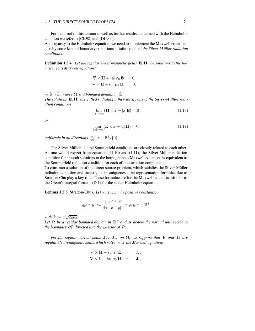
For the proof of this lemma as well as further results concerned with the Helmholtzequation we refer to [CK98] and [DL90a].Analogously to the Helmholtz equation, we need to supplement the Maxwell equationsalso by some kind of boundary conditions at infinity called the Silver-M uller radiationconditions.
Definition 1.2.4. Let the regular electromagnetic fields E,H, be solutions to the ho-mogeneous Maxwell equations
∇× H + iw ε0 E = 0,∇× E− iw µ0 H = 0,
in R3\Ω, where Ω is a bounded domain in R3.The solutions E,H, are called radiating if they satisfy one of the Silver-Mulller radi-ation conditions
lim|x|→∞
(H × x− |x|E) = 0 (1.18)
or
lim|x|→∞
(E× x+ |x|H) = 0, (1.19)
uniformly in all directions x|x| , x ∈ R3\0.
The Silver-Muller and the Sommerfeld conditions are closely related to each other.As one would expect from equations (1.10) and (1.11), the Silver-Muller radiationcondition for smooth solutions to the homogeneous Maxwell equations is equivalent tothe Sommerfeld radiation condition for each of the cartesian components.To construct a solution of the direct source problem, which satisfies the Silver-Mullerradiation condition and investigate its uniqueness, the representation formulae due toStratton-Chu play a key role. These formulae are for the Maxwell equations similar tothe Green’s integral formula (D.1) for the scalar Helmholtz equation.
Lemma 1.2.5 (Stratton-Chu). Let w, ε0, µ0 be positive constants,
gk(x, y) :=14π
eik|x−y|
|x− y| , x = y, x ∈ R3,
with k := w√ε0µ0.
Let Ω be a regular bounded domain in R3 and n denote the normal unit vector tothe boundary ∂Ω directed into the exterior of Ω.
For the regular current fields Je , Jm on Ω, we suppose that E and H areregular electromagnetic fields, which solve in Ω the Maxwell equations
∇× H + iw ε0 E = Je,
∇× E− iw µ0 H = −Jm.

22 CHAPTER 1. DIRECT ELECTROMAGNETIC SCATTERING
Then for x ∈ Ω we have
E(x) = iwµ0
∫Ω
gk(x, y)Je(y) dy
+∫
Ω
∇ygk(x, y) × Jm(y) dy
− i(wε0)−1
∫Ω
∇ygk(x, y)∇ · Je(y) dy
− iwµ0
∫∂Ω
gk(x, y) (n(y) × H(y)) dσ(y)
+∫
∂Ω
∇ygk(x, y) × (n(y) × E(y)) dσ(y)
−∫
∂Ω
∇ygk(x, y)(n(y) · E(y)) dσ(y), (1.20)
H(x) = iwε0
∫Ω
gk(x, y)Jm(y) dy
−∫
Ω
∇ygk(x, y) × Je(y) dy
− i(wµ0)−1
∫Ω
∇ygk(x, y)∇ · Jm(y) dy
+ iwε0
∫∂Ω
gk(x, y)(n(y) × E(y)) dσ(y)
+∫
∂Ω
∇ygk(x, y) × (n(y) × H(y)) dσ(y)
−∫
∂Ω
∇ygk(x, y)(n(y) · H(y)) dσ(y). (1.21)
For x ∈ R3\Ω the right hand side in (1.20) and (1.21) vanish identically.
We see from the Stratton-Chu representation formulae that the electromagneticfields, which are solutions to the Maxwell equations inside a regular bounded domainΩ ⊂ R3 with a smooth boundary ∂Ω, are completely determined from the volumedensities of electric and magnetic current sources Je and Jm in Ω and the value ofthe electromagnetic fields on the boundary ∂Ω . This suggests to consider two sub-problems called interior and exterior Maxwell problems, where the equations (1.5) and(1.6) are to be solved in Ω and in R3\Ω, respectively.The uniqueness of the solution to the Maxwell equations for prescribed boundary con-ditions follows immediately from the Stratton-Chu formulae.
Theorem 1.2.6. Let w, ε0 and µ0 be positive constants, Ω be a regular boundeddomain in R3 and n denote the normal unit vector to the boundary ∂Ω directed intothe exterior of Ω.

1.2. THE DIRECT SOURCE PROBLEM 23
We consider the homogeneous Maxwell equations
∇× H(x) + iw ε0 E(x) = 0, (1.22)
∇× E(x) − iw µ0 H(x) = 0. (1.23)
If E, H ∈ C(Ω)∩C1(Ω) are solutions to the homogeneous Maxwell equations in Ωsuch that
(n× E)(x) = (n × H)(x) = 0 for x ∈ ∂Ω, (1.24)
thenE = H = 0 in Ω.
If E, H ∈ C(R3\Ω)∩C1(R3\Ω) are radiating solutions to the homogeneousMaxwellequations in R3\Ω such that
(n × E)(x) = 0 for x ∈ ∂Ω, (1.25)
thenE = H = 0 in R3\Ω.
The proof of this theorem can be found in [Mue69]. It is to be noticed that for theexterior problem, an additional condition is assumed there, namely
E(x) = O
(1|x|
), |x| → ∞,
to hold uniformly in all directions x|x| , x ∈ R3\0.
However, this condition is systematically fulfilled by radiating solutions of the Maxwellequations, see [CK98].In the Stratton-Chu integral representations the electromagnetic fields E and H areexpressed in terms of their values on the boundary on the one hand, and in terms of theelectric and magnetic source densities Je, Jm and their divergence fields ∇ · Je, ∇ ·Jm on the other hand.If ρe(x, t) = e(x)e−iwt and ρm(x, t) = m(x)e−iwt are the volume densities ofelectric and ”magnetic” charges 4 in a position x ∈ R3 at a time t ∈ R, then from thecharge-conservation law we have the equations
∂ρe
∂t+ ∇ · Je = 0 and
∂ρm
∂t+ ∇ · Jm = 0,
which imply
e(x) = −iw−1∇ · Je and m(x) = −iw−1∇ · Jm.
Consequently, the volume integrals in the identities (1.20) and (1.21) relate the elec-tromagnetic fields to their electric and magnetic sources given as volume densities ofcurrents and charges.The question now is what the boundary integrals are due to.
4Magnetic charges are only virtual charges without actual physical existence.

24 CHAPTER 1. DIRECT ELECTROMAGNETIC SCATTERING
Theorem 1.2.7. Let w, ε0, µ0 be positive constants and
gk(x, y) :=14π
eik|x−y|
|x− y| , x = y, x, y ∈ R3,
with k := w√ε0µ0.
Let Ω be a regular bounded domain in R3 and n denote the normal unit vector tothe boundary ∂Ω directed into the exterior of Ω.If the complex-valued fields Je and Jm are regular current fields on Ω, vanishingoutside i.e. Je(x) = Jm(x) = 0 for x ∈ Ω.Then the fields E and H defined by
E(x) = iwµ0
∫Ω
gk(x, y)Je(y) dy
+∫
Ω
∇ygk(x, y) × Jm(y) dy
− i(wε0)−1
∫Ω
∇ygk(x, y) (∇y · Je(y)) dy
+ i(wε0)−1
∫∂Ω
∇ygk(x, y)(n(y) · Je(y)) dσ(y) (1.26)
H(x) = iwε0
∫Ω
gk(x, y)Jm(y) dy
−∫
Ω
∇ygk(x, y) × Je(y) dy
− i(wµ0)−1
∫Ω
∇ygk(x, y) (∇y · Jm(y)) dy
+ i(wµ0)−1
∫∂Ω
∇ygk(x, y)(n(y) · Jm(y)) dσ(y), (1.27)
are regular electromagnetic fields on Ω and R3\Ω, respectively, which satisfy
∇× H(x) + iw ε0 E(x) = Je(x) ,∇× E(x) − iw µ0 H(x) = −Jm(x),
for x ∈ Ω and
∇× H(x) + iw ε0 E(x) = 0,∇× E(x) − iw µ0 H(x) = 0.
for x ∈ R3\Ω.Moreover the fields E and H fulfill the Silver-Muller conditions.
We see from this theorem that discontinuities of the current fields Je and Jm,namely of their normal components,which occur through the boundary, are also sources

1.2. THE DIRECT SOURCE PROBLEM 25
of electromagnetic fields. These sources, called surface currents, are responsible forthe discontinuity of the fields E and H on the boundary.
Corollary 1.2.8. Let w, ε0, µ0 be positive constants and
gk(x, y) :=14π
eik|x−y|
|x− y| , x = y, x, y ∈ R3,
with k := w√ε0µ0.
Let Ω be a regular bounded domain in R3 and n denote the normal unit vector tothe boundary ∂Ω directed into the exterior of Ω.Let the complex-valued fields Je and Jm be regular current fields on Ω, vanishingoutside i.e.Je(x) = Jm(x) = 0 for x ∈ Ω.If we further suppose
n(y) · Je(y) = n(y) · Jm(y) = 0 for y ∈ ∂Ω. (1.28)
then the fields given by
E(x) = iwµ0
∫Ω
gk(x, y)Je(y) dy
+∫
Ω
∇ygk(x, y) × Jm(y) dy
− i(wε0)−1
∫Ω
∇ygk(x, y) (∇y · Je(y)) dy (1.29)
and
H(x) = iwε0
∫Ω
gk(x, y)Jm(y) dy
−∫
Ω
∇ygk(x, y) × Je(y) dy
− i(wµ0)−1
∫Ω
∇ygk(x, y) (∇y · Jm(y)) dy (1.30)
are in C1(R3,C3) and are radiating solutions to the Maxwell equations
∇× H + iw ε0 E = Je , (1.31)
∇× E− iw µ0 H = −Jm. (1.32)
For the proof of theorem 1.2.7 and Corollary 1.2.8 we refer to [Mue69]. The lastcorollary gives the solution of the direct source problem as a sum of three volume in-tegrals. The electric field can be seen as generated by three types of volume sources.The first integral shows the radiation of the volume density of electrical currents, thesecond integral reflects the contribution due to the electromagnetic coupling and thelast one is the contribution due to the volume density of electrical charges. A similarinterpretation is also valid for the magnetic field.To guarantees the regularity of the electromagnetic fields we made an assumption ex-cluding surface currents in our modeling of the direct source problem. For more detailsabout the effects of the surface currents we refer to [VB91].

26 CHAPTER 1. DIRECT ELECTROMAGNETIC SCATTERING
1.3 The direct medium problem
In this section we deal with the determination of electromagnetic fields in an inho-mogeneous medium excited by an extraneous incident field when the electromagneticmaterial properties are prescribed. In the first subsection, we use the concept of inducedor equivalent sources to reduce the direct medium problem into a direct source prob-lem. We then derive the formulation as a system of integro-differential equations. Inthe second section we give the formulation of the direct medium problem as a boundaryvalue problem and state existence and uniqueness result in a weaker space setting. Thisformulation is relevant as far as inversion from boundary measurement is concerned.In the last section we define the operator formalism used throughout this work. Theequations of Lippmann-Schwinger type give a unified setting for modeling scatteringin inhomogeneous media and highlights the similarities between scattering problemsin acoustics and in electromagnetics.
1.3.1 Integral equation formulation
Let Ω be a regular bounded domain in R3 with boundary ∂Ω, w > 0 be a fixedfrequency and ε0, µ0, be positive constants .For an inhomogeneous medium with prescribed electromagnetic properties ε and µsatisfying
ε− ε0, µ− µ0 ∈ C10 (Ω,C) (1.33)
withRe(ε) > 0, Re(µ) > 0, (1.34)
we consider the following direct medium problem.Let Ei,Hi ∈ C1(R3,C3) be solutions in R3 to the homogeneous Maxwell equations
∇× Hi + iw ε0 Ei = 0, (1.35)
∇× Ei − iw µ0 Hi = 0. (1.36)
We want to find E,H ∈ C1(R3,C3) which are solutions to the Maxwell equations
∇× H + iw εE = 0, (1.37)
∇× E − iw µH = 0, (1.38)
in R3, such that the scattered fields Es and Hs defined by
Es : = E− Ei, (1.39)
Hs : = H− Hi, (1.40)
satisfy the Silver-Muller radiation condition
lim|x|→∞
(Hs × x− |x|Es) = 0. (1.41)

1.3. THE DIRECT MEDIUM PROBLEM 27
If we introduce the induced electric and magnetic current sources Je and Jm definedby
Je := iw(ε0 − ε)E, (1.42)
Jm := iw(µ0 − µ)H, (1.43)
the direct medium problem is then reduced to a direct source problem in homogeneousmedium for the induced source densities Je and Jm . Indeed, From the equations(1.35)-(1.43) we get
∇× Hs + iw ε0 Es = Je , (1.44)
∇× Es − iw µ0 Hs = −Jm, (1.45)
where the scattered fields Es, Hs have to satisfy the radiating condition (1.41).If we denote
gk(x, y) :=14π
eik|x−y|
|x− y| , x = y, x ∈ R3.
with k := w√ε0µ0, we get from Corollary 1.2.8 that the electromagnetic fields given
by
E(x) = Ei(x) + iwµ0
∫Ω
gk(x, y)Je(y) dy
+∫
Ω
∇ygk(x, y) × Jm(y) dy
− i(wε0)−1
∫Ω
∇ygk(x, y) (∇y · Je(y)) dy (1.46)
and
H(x) = Hi(x) + iwε0
∫Ω
gk(x, y)Jm(y) dy
−∫
Ω
∇ygk(x, y) × Je(y) dy
− i(wµ0)−1
∫Ω
∇ygk(x, y) (∇y · Jm(y)) dy, (1.47)
are solutions to the direct medium problem.Inversely, the solutions to the integral equation (1.46) and (1.47) are also solutions tothe Maxwell equations as we can see from the next theorem.
Theorem 1.3.1. Let ε, µ satisfy the conditions (1.33),(1.34)and E i,Hi ∈ C1(R3,C3)be solution in R3 to the homogeneous Maxwell equations (1.35)-(1.36).

28 CHAPTER 1. DIRECT ELECTROMAGNETIC SCATTERING
If E, H ∈ C(R3,C3) are solutions to the integral equations
E(x) = Ei(x) − w2µ0
∫Ω
gk(x, y) (ε0 − ε(y))E(y) dy
+ iw
∫Ω
∇ygk(x, y) × (µ0 − µ(y))H(y) dy
−∫
Ω
∇ygk(x, y) (∇εε
(y) ·E(y)) dy (1.48)
and
H(x) = Hi(x) − w2ε0
∫Ω
gk(x, y)(µ0 − µ(y))H(y) dy
− iw
∫Ω
∇ygk(x, y) × (ε0 − ε(y))E(y)) dy
−∫
Ω
∇ygk(x, y) (∇µµ
(y) · H(y)) dy, (1.49)
for x ∈ R3, then we have
∇ · (ε0 − ε)E = −ε0∇εε
· E, (1.50)
∇ · (µ0 − µ)H = −µ0∇µµ
· H. (1.51)
Furthermore, E and H are in C1(R3,C3) and the scattered fields
Es : = E− Ei, (1.52)
Hs : = H− Hi, (1.53)
are radiating solution to the Maxwell equations
∇× Hs + iw ε0 Es = Je , (1.54)
∇× Es − iw µ0 Hs = −Jm, (1.55)
in R3 with
Je := iw(ε0 − ε)E, (1.56)
Jm := iw(µ0 − µ)H. (1.57)
Remark. The relations (1.50) and (1.51) following from the integral equations (1.48)and (1.49) are necessary to derive the Maxwell-equations from the equations (1.46) and(1.47).
The scattering of electromagnetic fields from an inhomogeneous medium with pre-scribed electromagnetic properties and given incident fields is governed by a system ofintegro-differential equations. The contrast of the electromagnetic properties betweenan object and its background creates equivalent sources of currents and charges. Thescattered electromagnetic field is interpreted as being radiated from these sources.
1.3. THE DIRECT MEDIUM PROBLEM 29
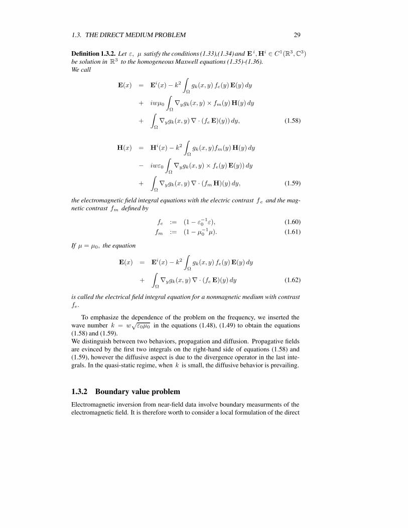
Definition 1.3.2. Let ε, µ satisfy the conditions (1.33),(1.34)and E i,Hi ∈ C1(R3,C3)be solution in R3 to the homogeneous Maxwell equations (1.35)-(1.36).We call
E(x) = Ei(x) − k2
∫Ω
gk(x, y) fe(y)E(y) dy
+ iwµ0
∫Ω
∇ygk(x, y) × fm(y)H(y) dy
+∫
Ω
∇ygk(x, y)∇ · (fe E)(y)) dy, (1.58)
H(x) = Hi(x) − k2
∫Ω
gk(x, y)fm(y)H(y) dy
− iwε0
∫Ω
∇ygk(x, y) × fe(y)E(y)) dy
+∫
Ω
∇ygk(x, y)∇ · (fm H)(y) dy, (1.59)
the electromagnetic field integral equations with the electric contrast fe and the mag-netic contrast fm defined by
fe := (1 − ε−10 ε), (1.60)
fm := (1 − µ−10 µ). (1.61)
If µ = µ0, the equation
E(x) = Ei(x) − k2
∫Ω
gk(x, y) fe(y)E(y) dy
+∫
Ω
∇ygk(x, y)∇ · (fe E)(y) dy (1.62)
is called the electrical field integral equation for a nonmagnetic medium with contrastfe.
To emphasize the dependence of the problem on the frequency, we inserted thewave number k = w
√ε0µ0 in the equations (1.48), (1.49) to obtain the equations
(1.58) and (1.59).We distinguish between two behaviors, propagation and diffusion. Propagative fieldsare evinced by the first two integrals on the right-hand side of equations (1.58) and(1.59), however the diffusive aspect is due to the divergence operator in the last inte-grals. In the quasi-static regime, when k is small, the diffusive behavior is prevailing.
1.3.2 Boundary value problem
Electromagnetic inversion from near-field data involve boundary measurments of theelectromagnetic field. It is therefore worth to consider a local formulation of the direct

30 CHAPTER 1. DIRECT ELECTROMAGNETIC SCATTERING
medium problem as a boundary value problem.Furthermore, the uniqueness result for the inverse medium problem relies on the weakformulation of the direct problem. For the functional space setting, we use the Sobolevspaces, Hs, s ∈ R, as they are defined in [DL88]. For the sake of clarity, we use thenotations grad, div andcurl for the gradient, divergence and curl operators in theweak sense and we denote Div the surface divergence 5 operator.Let Ω ⊂ R3 be a bounded domain with a smooth boundary Γ. For x ∈ Γ, let n(x),denote the outward normal unit vector to the boundary.
Definition 1.3.3. For s ∈ R, we define
THs(Γ) := f ∈ Hs(Γ)3, n · f = 0
as the Sobolev space of tangential fields.For s ≥ 1, we define the space
THsDiv(Γ) := f ∈ THs(Γ)3, Div f ∈ Hs(Γ),
endowed with the norm
||f ||THsDiv(Γ) := ||f ||Hs(Γ)3 + ||Div f ||Hs(Γ),
and the space
HsDiv(Ω) := f ∈ Hs(Ω)3, Div(n × f|Γ) ∈ Hs− 1
2 (Γ),
endowed with the norm
||f ||HsDiv(Ω) := ||f ||Hs(Γ)3 + ||Div f ||Hs(Γ).
The spaces HsDiv(Ω) arise naturally through the tangential trace mapping on the
boundary, see D.0.11.
Theorem 1.3.4. Let w, ε0 and µ0 be positive contants, ε and µ satisfy
ε− ε0 ∈ C10 (Ω,C), µ− µ0 ∈ C1
0 (Ω,R) (1.63)
withRe(ε) > 0, Im(ε) > 0, µ > 0, (1.64)
Then the boundary value problem
curlH + iw εE = 0,curlE− iw µH = 0,
with the boundary condition
n × E = f on Γ (1.65)
for given f ∈ TH12Div(Γ),
admits a unique (weak) solution (E,H) ∈ H 1Div(Ω) ×H1
Div(Ω).5for more details about the surface divergence we refer to [CK98] p.167.

1.4. EQUATION OF LIPPMANN-SCHWINGER TYPE 31
This result can be found in [Isa98] p. 137. If Im(ε) = 0, theorem 1.3.4 holdsexcept for a discrete set of resonance frequencies wnn.We see from theorem 1.3.4 that the direct medium problem formulated as a boundaryvalue problem is uniquely solvable if the tangential component of the electrical field isprescribed on the boundary. A similar result can be derived if the tangential componentof the magnetic field is prescribed on the boundary.
1.4 Equation of Lippmann-Schwinger type
For w, ε, µ and k positive constants with k := w√εµ, let
gk(x, y) :=14π
eik|x−y|
|x− y| , x = y, x ∈ R3,
and Ω, Ω′, Ω ⊂ Ω′, be two bounded domains in R3 with smooth boundaries.
Definition 1.4.1. The (first) scalar scattering operator A is defined for f ∈ C0(Ω) by
Af(x) :=∫
Ω
gk (x, y) f(y) dy, x ∈ R3.
The second scalar scattering operator A′
is defined 6 for f ∈ C0(Ω) by
A′f(x) :=
∫Ω
∇y gk (x, y) f(y) dy, x ∈ R3.
For N ∈ N, N > 1, the vector scattering operator A is defined for f = (fi)i=1,..,N ∈C0(Ω)N by
Af := (Afi)i=1,..,N .
The first coupling operator Kd is defined for f ∈ C10 (Ω)3 by
Kd f(x) :=∫
Ω
∇y gk (x, y)div f (y) dy, x ∈ R3.
The second coupling operator Kr is defined for f ∈ C0(Ω)3 by
Kr f(x) :=∫
Ω
∇y gk (x, y) × f(y) dy, x ∈ R3.
Hilbert-spaces provide a better setting for the inverse problem. Before extendingthe operators defined above onto spaces of square integrable functions, we recall thedefinition of some spaces, for more details see [DL88].
6The notation should not be confused with the usual notation for the derivative.

32 CHAPTER 1. DIRECT ELECTROMAGNETIC SCATTERING
Definition 1.4.2. We define the space
H(div,Ω) := f ∈ L2(Ω)3, div f ∈ L2(Ω),
endowed with the norm
||f ||H(div,Ω) :=(||f ||2L2(Ω)3 + ||div f ||2L2(Ω)
) 12,
and the spaceH(curl,Ω) := f ∈ L2(Ω)3, curl f ∈ L2(Ω),
endowed with the norm
||f ||H(curl,Ω) :=(||f ||2L2(Ω)3 + ||curl f ||2L2(Ω)3
) 12.
We denoteH(div0,Ω) := f ∈ L2(Ω)3, div f = 0
andH(curl0,Ω) := f ∈ L2(Ω)3, curl f = 0.
The closure of C∞0 (Ω) in Hs(Ω), s ∈ R, is denoted Hs
0(Ω). The closure of C∞0 (Ω)3
inH(div,Ω) is denoted H0(div,Ω) and inH(curl,Ω) is denoted H0(curl,Ω).
Lemma 1.4.3. We can extend the operators defined above to
1. A ∈ L (L2 (Ω), H2 (Ω′)).
2. A′ ∈ L (L2 (Ω), H1 (Ω
′)3).
3. A ∈ L (L2 (Ω)N , H2 (Ω′)N ).
4. Kd ∈ L (H (div,Ω), H (curl0,Ω′) ∩H1(Ω
′)3).
5. Kr ∈ L (L2 (Ω), H1 (div0,Ω′)).
Proof. The first assertion is proved in [CK98] p.215 and it immediately implies thethird one.The second assertion may be proved similarly to the first one, where the kernel g k (x, y)is replaced by ∇y gk (x, y), which is also weakly singular.In the fourth assertion, the operator Kd can be extended boundedly, since A ′ isbounded and we have
||Kdf ||H1(Ω)3 ≤ ||A′|| ||div f ||L2(Ω) ≤ ||A′|| ||f ||H (div,Ω) for f ∈ H (div,Ω).
It remains to show that
curlKd f = 0 for f ∈ H (div,Ω).

1.4. EQUATION OF LIPPMANN-SCHWINGER TYPE 33
Let f ∈ L2 (Ω) , gradAf makes sense since Af ∈ H2(Ω′) .
Using the identity
∇x gk (x, y) =14π
eik|x−y|
|x− y|
(1
|x− y| − ik
)y − x
|x− y| = −∇y gk (x, y), x = y,
we get
gradAf(x) = ∇x
∫Ω
gk (x, y) f(y)dy = −∫
Ω
∇y gk (x, y) f(y)dy = −A′f(x)
forx ∈ Ω′. It yields
gradA = −A′
on L2 (Ω).
For f ∈ H (div,Ω), we have
Kd f(x) = −gradAdiv f(x) for x ∈ Ω′,
and concludeR(Kd) ⊂ N (curl).
We have Kr ∈ L (L2 (Ω), H1 (Ω′)3) as A
′ ∈ L (L2 (Ω), H1 (Ω′)).
Let f ∈ C10 (Ω) and x ∈ Ω′. From the identity
curl (gk(x, y)f(y)) = ∇y gk(x, y) × f(y) + gk(x, y) curl f(y), y ∈ Ω, y = x,
and as the integral of the left-hand side vanishes by virtue of the curl theorem, see forexample [DL90b] p.311, we get
Krf(x) =∫
Ω
∇y gk (x, y) × f(y) dy
= −∫
Ω
∇x gk (x, y) × f(y) dy
= −∫
Ω
∇x × (gk (x, y) f(y)) dy
= −∇x ×∫
Ω
gk (x, y) f(y) dy
= −curlA f(x), x ∈ Ω.
Since C10 (Ω) is dense in L2 (Ω), we get
Kr = −curlA on L2 (Ω),
and consequentlyR(Kr) ⊂ N (div).
We collect some intermediate results from the proof above in the following corol-lary.

34 CHAPTER 1. DIRECT ELECTROMAGNETIC SCATTERING
Corollary 1.4.4. We have
gradA = −A′
on L2(Ω),Kd = −gradAdiv on H(div,Ω),
Kr = −curlA on L2(Ω)3.
Definition 1.4.5. The electromagnetic scattering operator Tem is defined for f =(fe, fm) ∈ C1
0 (Ω)3 × C10 (Ω)3 by
Tem f := (Te f , Tm f)
with
Te f = k2 Afe − Kd fe − i ω µ0 Kr fm, (1.66)
Tm f = k2 Afm − Kd fm + i ω ε0 Kr fe. (1.67)
The nonmagnetic scattering operator Te is defined for f ∈ C10 (Ω)3 by
Te f = k2 Af − Kd f . (1.68)
Lemma 1.4.6. The nonmagnetic scattering operator Te can be extended to a boundedlinear operator from H (div,Ω) to L2 (Ω
′)3.
The electromagnetic scattering operator Tem can be extended to a bounded linear op-erator from H (div,Ω) ×H (div,Ω) to L2 (Ω
′)3 × L2 (Ω
′)3.
Definition 1.4.7. Let n ∈ N, X be a Banach-algebra and T ∈ L(X N ).For fixed f ∈ X and u0 ∈ XN , the equation
u = u0 − Tfu, u ∈ XN , (1.69)
is said to be of Lippmann-Schwinger type for T.Let V ⊂ X . If for every f ∈ V and u0 ∈ XN , the equation (1.69) admits a uniquesolution u, the nonlinear operator A defined on V ×X N by
A (f, u0) = u
is called a Lippmann-Schwinger operator for T.
Examples
1. The scattering of time-harmonic acoustic waves in an inhomogeneous mediumis modeled by an integral equation of Lippmann-Schwinger type with N =1, X = C (Ω) for the operatorT = k2A, k > 0, where A is the scalar scatteringoperator, see [CK98] p. 216. This equation is refered to as the scalar Lippmann-Schwinger equation.
2. Let N = 3,X = C1 (Ω) × C1 (Ω). The system of electromagnetic equations isof Lippmann-Schwinger type for the operator T = T em with
u0 := (Ei, Hi), u := (E,H), f := (fe, fm).
We call this equation the electromagnetic Lippmann-Schwinger equation.

1.4. EQUATION OF LIPPMANN-SCHWINGER TYPE 35
3. LetN = 3,X ∈ C1 (Ω). The electrical field integral equation for a nonmagneticmedium with contrast fe is of Lippmann-Schwinger type for the operator T =Te with
u0 := Ei, u := E, f := fe.
We call this equation the nonmagnetic Lippmann-Schwinger equation.
Theorem 1.4.8. (Well-posedness of the direct medium problem)
1. Let X = C (Ω). For f ∈ C1,α(Ω) with compact support in Ω, α ∈ (0, 1), thereexists a unique solution u ∈ X to the scalar Lippmann-Schwinger equation andthis solution depends continuously with respect to the maximum norm on theincident field u0 ∈ X .
2. Let X = C1 (Ω)3 × C1 (Ω)3. For f ∈ C1,α(Ω) × C1,α(Ω) with compactsupport in Ω, α ∈ (0, 1), there exists a unique solution u ∈ X to the electro-magnetic Lippmann-Schwinger equation and this solution depends continuouslywith respect to the maximum norm on the incident field u0 ∈ X .
3. Let X = C1 (Ω)3. For f ∈ C1,α(Ω) with compact support in Ω, α ∈ (0, 1),there exists a unique solution u ∈ X to the nonmagnetic Lippmann-Schwingerequation and this solution depends continuously with respect to the maximumnorm on the incident field u0 ∈ X .
Proof. The proof of the first assertion can be found in [CK98]. For the proof of thethird one see [Mue69], the second assertion is a particular case of it.
Remarks.
1. We lose no generality when we restrict the Lippmann-Schwinger equations tothe bounded domain Ω, instead of the whole space R3 , since the values of thefields outside Ω are completely determined from the values of the fields on Ω byusing the integral operator.
2. For the analysis of the nonmagnetic Lippmann-Schwinger operator in the settingof Sobolev spaces we refer to [AB01].
3. The Helmholtz operator ∆ + k2 acting componentwise on vector wave fieldscan be seen as the scalar approximation to the operator −∇×∇ + k 2.This assumption is particularly valid for fields with weak divergence. Neverthe-less, there is an essential difference between the two operators. The Helmholzoperator is elliptic, however the operator −∇×∇ + k 2 is not.
4. Although the discretized form of the integral equations does not lead to sparsematrices like the partial differential equations do, it is advantageous to use theLippmann-Schwinger equation to model the forward problem since the bound-ary conditions are already embedded in the integral equation formulation. Fur-thermore many properties of elliptic partial differential equations, such as theLax-Milgram lemma, are not valid for the non-elliptic Maxwell-Model.

36 CHAPTER 1. DIRECT ELECTROMAGNETIC SCATTERING

Chapter 2
Inverse electromagneticscattering
Inverse scattering is a central problem in diverse areas of application. The goal isthe determination of the characteristics, like the shape, location, acoustic or electro-magnetic constitutive properties, of a buried object embedded in some known back-ground. We are intereseted in the inversion carried from near-filed measurements ofthe scattered waves using sensors placed outside the target-object illuminated by aset of monochromatic incident fields. For the scattering of electromagnetic waves,we base our modeling on the contrast source integral equations corresponding to fullthree-dimensional Maxwell equations. The formulation as equations of Lippmann-Schwinger type on hand for the Helmholtz and the Maxwell models provides a com-prehensive framework for inverse scattering problems in inhomogeneous media foracoustic and electromagnetic waves.We start this chapter with an abstract formulation of the inverse scattering problems.We next highlight the practical relevance of the electromagnetic inverse scattering anddiscuss some methods to accomplish the inversion. We further present for the inversemedium problem a uniqueness result due to Ola, Paivarinta and Somersalo. In thethird section, we introduce a procedure to make the inversion of the electromagneticand nonmagnetic scattering operators. The last section is devoted to treat the scalarscattering operator when the geometrical configuration is spherical.
2.1 Formulation of the inverse problems
The bounded domain Ω ⊂ R3 with a smooth boundary ∂Ω, denotes the target regionwhere the material parameters are to be determined. The contrast functions are sup-posed to be compactly supported in Ω and are elements of the parameter space V (Ω),which can be injected into a subspace of L2 (Ω)N . The N-dimensional wave fields areelements of the state space U (Ω)N ⊂ L2 (Ω)N . Let the source space X (Ω)N be asubspace of L2 (Ω)N such that f u ∈ X (Ω)N for every f ∈ V (Ω) and u ∈ U (Ω)N .The data are measured on the subset Γ of R3, which is in general a surface exterior
37

38 CHAPTER 2. INVERSE ELECTROMAGNETIC SCATTERING
to the target region. The data space Y (Γ)P is a subspace of L2 (Γ)P . We notice thatin many experimental setting, the dimension P of the measured data may differ fromthe dimension of the wave fields N.The scattering operator denoted by T : X (Ω)N → U (Ω)N associates to a source φthe scattered field us := Tφ.Let I ⊂ N denote the experiment-set with p elements. For each j ∈ I , we are given anoperatorM j : U (Ω)N → Y (Γ)P called the measurement operator for the j th- exper-iment, which to an element uj from the state-space U (Ω)N associates an element dj
from the data-space Y (Γ)P .The operator T j
Γ = M jT is called the restricted scattering operator.
Definition 2.1.1. For j ∈ I, let the incident fields vj ∈ U (Ω)N be given. The inversemedium problem for the operator T and the measurement operators (M j)j ∈ I reads :To the data dj ∈ Y (Γ)P , determine the contrast function f ∈ V (Ω), such that thereexists a wave field uj ∈ U (Ω)N satisfying the data fitting equation and the equationof Lippmann-Schwinger type given by the system:
M jusj = dj ,
usj = T (f uj),
with usj := uj − vj , for every j ∈ I.
We can already see two major difficulties featuring the inverse medium problem ingeneral:
• The ill-posedness, which is typical for inverse problems. It is here twofold sincethe inverse problem is under-determinedand ill-conditioned. In general, the mea-surements are taken on a subset Γ, which can be immersed in a manifold oflower order than the target region Ω. The operator MΓ T admits, therefore, abig null space. Furthermore, data are endowed with an unavoidable error, whichare related to measurement conditions. This causes instability when making theinversion.
• The nonlinearity. The dependence of the field u on the contrast function f is inmany applications highly nonlinear.
In comparison with the acoustic case, the electromagnetic case presents mainly twofurther aspects of difficulty:
• Mathematically, the system is much more complicated since the underlying oper-ators are integro-differential operators acting on three-dimensional vector fields.Furthermore, all components of the vector fields are intertwined, which requiresthe simultaneous treatment of all components.
• Physically, besides the propagation, a diffusive behavior and an electromagneticcoupling are involved.

2.2. APPLICATIONS AND METHODS OF INVERSION 39
Definition 2.1.2. If the contrast function f and the total field (u j)j are solution tothe inverse medium problem, then φj := f uj, j ∈ I , is called equivalent or induced(current) source for the jth-experiment.The determination of the equivalent source φj , j ∈ I , satisfying
T jΓφj = dj
is called inverse source problem for the j th-experiment.
We see that the solution of the inverse medium problem provides the contrast functionf as an identification parameter for the material, which should be the same for allexperiments j ∈ I . The total wave field uj and the induced source φj = f uj are,however, depending on the experiment j. For each j ∈ I we have a new inverse sourceproblem.
2.2 Applications and methods of inversion
Inversion algorithms are closely related to the field of application and to technologicalconsiderations. Technical limitations usually compromise the expectations of the inver-sion method and its relevance for practice. The acting frequency, the size and strengthof the scatterer, the measurement conditions are crucial criteria for the modeling andinversion of electromagnetic data, see [dH00], [NH00].
Microwave tomography is a competitive noninvasive imaging technique in severalpractical areas. For medical application, microwave radiation can be used, withoutas much caution as for x-ray tomography, to identify the properties and to detect theanomalies of biological tissues by determining the electromagnetic characteristics likethe electric permittivity and conductivity, see [SBS+00]. The operating frequenciesare typically in GHz range, [Kon90] p.13. The resolution is, however, not as accurateas the x-ray tomography since it does never provide the millimeter precision reachedwhen using high-energetic radiations.
For geophysical prospecting, popular devices are the ground penetrating radars(GPR). They operate at frequencies ranging from radio to microwave domain, typi-cally larger than 100 MHz, see [DBABC99]. Due to the attenuation of the wave atthese frequencies, the underground penetration remains limited.Alternatively, one may use metal detectors operating at the lower frequency-band of ra-dio waves (≤ 300 KHz). This involves electromagnetic induction tomography, whichis a promising tool for imaging electromagnetic parameters like the electrical conduc-tivity with relevance for many practical problems, such as the recent application tohumanitarian mine detection. Nevertheless, a typical feature for this tomographicalmethod in comparison with the microwave imaging is the diffusive character of thewaves. Therefore, the treatment of the full three-dimensional Maxwell Model is re-quired.

40 CHAPTER 2. INVERSE ELECTROMAGNETIC SCATTERING
Many linear inversion methods are based on the Born/Rytov approximation, see[Lan87], where the scattered field is neglected with respect to the incident field. Thisleads to a linearized model for the scattering, whose validity is, however, confinedto scatterers with low-contrast. Electromagnetic imaging involving techniques fromthe diffraction tomography, see [Nat01], [NW01], [KS88], are based on linear modelsusing Born approximation or further extensions of it like the iterated Born approxima-tion, or relying on empirical approximation such as the quasi-analytical method due toZdhanov [Zhd02] or the synthetic aperture focusing techniques used in [MMH +02].These methods remain with limited scope of application. The treatment of the nonlin-ear model is therefore necessary.
The approach in [NH00], [NB04], [Hab04], is to use nonlinear optimization tech-niques to reduce the mismatch between measured data and the predicted fields as afunctional of the sought-for material parameters. In their iterative method, the highcost of the full Newton iteration is circumvented by using some approximation of theJacobian. This leads to a scheme of Quasi-Newton type. Discretized Maxwell’s equa-tions are used for the forward model.
Dorn et al. in [DBABC99], [DBABP02], derive a nonlinear inversion of electro-magnetic data for geophysical applications using the adjoint operator of the Frechetderivative of the residual operator. Their iterative scheme can be considered as a gen-eralization to nonlinear problems of the algebraic reconstruction technique for linearsystems (ART) in x-ray tomography. The nonlinear iterations rely on a forward solverof the boundary value problem for the Maxwell equations. The method of Vogeler[Voe03] for microwave tomography utilizes also similar techniques. The modeling ofthe forward problem is alternatively formulated there as an initial value problem.
The source-type methods consist in the splitting of the nonlinear inverse mediumscattering problem into two subproblems. The first one is the inverse source problem.It is linear but ill-posed. One attempts here, to recover the equivalent sources realiz-ing the best fitting to the data. The second problem is in general well-posed, howevernonlinear. It consists in the derivation of the material properties from the recoveredequivalent source by solving the constitutive relations. Although, the equivalent sourcemay already provide a good guess about the scatterer, see [AL99], [DMR00], the fullreconstruction of the material properties from the equivalent source recovered from asingle experiment is in general unfeasible. This is due to the non uniqueness of the so-lution of the inverse source problem related to the existence of non-radiating sources.These are sources φj that generate scattered fields us
j with M jus = 0. Non-radiatingsources and the fields they generate have been investigated for many years as a typicalfeature of the inverse source problem for the Helmholtz and the Maxwell equations,see [DW73], [BC77], [CWO+94], [DM98]. Hence, to recover the contrast functionone should combine the outcome of many experiments.
Many algorithms to solve the inverse scattering problem for the Helmholtz or theMaxwell equations can be considered as source-type inversion. One approach is touse the resolution of the inverse source problem as a built-in component of an it-

2.3. UNIQUENESS 41
erative algorithm. Typical examples, in the framework of the contrast source inte-gral equation in two dimensional case, are the method of Habashy et al. [HGS93],[HODH95], and the contrast source inversion method due to van den Berg and Klein-mann [vdBK97],[vdB01]. Some of these Methods have been already extended to theelectromagnetic case, see [AvdB02] and [BSSP04]. A common feature of all theseschemes is the simultaneous treatment of all data and the resolution of the forwardproblem in each iteration, which obviously enhance the computation and storage ef-fort dramatically. Abdullah and Louis [AL99] and later Wallacher [Wal02] proceededdifferently. They first made a linear inversion to compute an approximate value of theequivalent source, which corresponds to the component with minimal energy calledthe minimal-norm solution. On a subspace orthogonal to the recovered component, anonlinear optimization is executed to compute the contrast function, which realizes thebest fitting for all experiments, see also [HODH95]. The optimization is accomplishedwith respect to an analytically precomputed basis. This means that no forward compu-tation is required within the iterations of the nonlinear part of the scheme. The pricefor that is to determine the singular value decomposition of the restricted scatteringoperator T j
Γ and a basis for its null space. The linear inversion is regularized usingthe approximate inverse. It yields, therefore, a stable and efficient scheme for the twodimensional case, which also works within a setting of incomplete data [Wal02].
2.3 Uniqueness
We present in this section a uniqueness theorem for the inverse medium problem for-mulated as a boundary value problem for the Maxwell’s equations. This result is dueto Ola, Paivarinta and Somersalo, see [OPS93], [OS96]. The proof for the electro-magnetic case can be seen as an extension of the uniqueness theorem developed bySylvester Uhlman [SU87] and Nachmann [Nac88] for the inverse conductivity prob-lem in two-dimension. The global uniqueness theorem, derived there, states that thematerial parameters are uniquely determined from the Dirichlet-to-Neumann map. Inthe electromagnetic case the impedance map plays the role played by the Dirichlet-to-Neumann map in scalar inverse problems.
Definition 2.3.1. Let w, ε0 and µ0 be positive constants, ε and µ satisfy
ε− ε0 ∈ C10 (Ω,C), µ− µ0 ∈ C1
0 (Ω,R)
with
Re(ε) > 0, Im(ε) > 0, µ > 0.
The impedance map is defined by
Z : TH12Div(Γ) −→ TH
12Div(Γ)
f −→ n× E,

42 CHAPTER 2. INVERSE ELECTROMAGNETIC SCATTERING
such that (E,H) ∈ H1Div(Ω) ×H1
Div(Ω) are solutions to the Maxwell equations
curlH + iw εE = 0, (2.1)
curlE− iw µH = 0, (2.2)
with the boundary condition
n× H = f on Γ. (2.3)
Theorem 2.3.2. The impedence map Z determines uniquely the coefficients ε, µ withthe above properties.
Besides the theoretical importance of theorem 2.3.2, it shows the amount of data re-quired to uniquely reconstruct the electromagnetic properties of a medium from bound-ary measurements.Further results on uniqueness of inverse scattering can be found in [Isa01]. For elec-tromagnetic inversion from local surface measurements see [Liu99].
2.4 Inversion of the em-scattering operators
In this section, we introduce a new procedure based on the concept of generalized in-duced sources. It plays a key role in the method developed in this work.As before mentioned, the system modeling electromagnetic scattering involves integro-differential operators acting on vector fields with intertwined components, which re-quires a simultaneous treatment of all equations of the system. To decouple this system,we define the electromagnetic and nonmagnetic scattering potentials. This generalizesthe concept of equivalent current sources, where the diffusion and the electromagneticcoupling are also considered. Using the introduced potentials, we derive a factoriza-tion of the electromagnetic and nonmagnetic scattering operators. As a consequence,we can recast the inverse electromagnetic scattering into a scalar inverse source prob-lem for each component of the field.Besides the decoupling of the underlying equations in the electromagnetic case, we usethe described procedure to develop, in section 4 of the third chapter, an iterative schemeto solve the nonlinear inverse medium problem.
We begin first with the next lemma. The identities given there can be seen as ageneralization of the Green’s formulea to vector fields.
Lemma 2.4.1. Let Ω be a bounded domain in R3 with a smooth boundary ∂Ω andn(x) denote the unit vector normal to the boundary at x ∈ ∂Ω. Then we have∫
Ω
v(x) · gradϕ(x) dx = −∫
Ω
div v(x)ϕ(x) dx +∫
∂Ω
v(x) · n(x)ϕ(x) dσ(x)
for v ∈ H (div,Ω), ϕ ∈ H1(Ω) and∫Ω
u(x) · curl v(x) dx =∫
Ω
curl u(x) ·v(x) dx +∫
∂Ω
[u(x) ∧ n(x)] ·v(x) dσ(x)

2.4. INVERSION OF THE EM-SCATTERING OPERATORS 43
for u ∈ H (curl,Ω), v ∈ H1(Ω)3.
Proof. For the proof of this lemma we refer to [DL90b] p. 206 and p. 207.
Let w, ε, µ be positive constants and
gk(x, y) := gk(|x − y|) =14π
eik|x−y|
|x− y| , x = y, x ∈ R3,
with k := w√εµ.
Lemma 2.4.2. If Ω is a bounded domain in R3 with a smooth boundary, then∫Ω
curl (gk(x, y) f(y)) dy = 0 for f ∈ H10 (Ω)3, (2.6)∫
Ω
grad (gk(x, y) f(y)) dy = 0 for f ∈ H10 (Ω). (2.7)
Proof. Let f ∈ C∞0 (Ω)3 whose support is contained in a compact set K ⊂ Ω with a
smooth boundary ∂K .Let x ∈ R3, x ∈ ∂K, Bε denote a ball, with center x and radius ε > 0, contained inK if x ∈ K and Bε = ∅ if x ∈ K. Further, let Kε := K Bε and (ei)i=1,2,3 be thecanonical basis in R3.Let n(y) denote the outward unit vector normal to the boundary at y ∈ ∂B ε ∪ ∂K.If we apply the second identity from lemma 2.4.1 to u = e i, i ∈ 1, 2, 3, and v(y) :=gk(x, y) f(y) ∈ H1(Kε), we get∫
Kε
∇y × (gk(x, y) f(y)) · ei dy =∫
∂Bε
gk(x, y) f(y) · (ei ∧ n(y)) dσ(y),
since ei is constant and∫∂K
gk(x, y) f(y) · (ei ∧ n(y)) dσ(y) = 0
for f ∈ C∞0 (K)3.
From the inequalities
|a · b| ≤ |a||b|, |a ∧ b| ≤ |a||b| for a,b ∈ R3,
and|gk(x, y)| = (4πε)−1, y ∈ ∂Bε,
we obtain the estimate∣∣∣∣∫∂Bε
gk(x, y) [ f(y) · (ei ∧ n(y)) ] dσ(y)∣∣∣∣ ≤ ‖f‖∞
∫∂Bε
|(gk(x, y)| dσ(y)
= ε‖f‖∞.

44 CHAPTER 2. INVERSE ELECTROMAGNETIC SCATTERING
When ε tends to zero, we get∫K
curl(gk(x, y) f(y)
)·ei dy = 0, for i ∈ 1, 2, 3. (2.8)
The first formula has been proved for f ∈ C∞0 (Ω)3. By a density argument it also
holds for f ∈ H10 (Ω)3.
To prove the second identity, we proceed similarly to above by applying the first for-mula from lemma 2.4.1 to v = ei and ϕ(y) = gk(x, y) f(y) for f ∈ H1
0 (Ω).
We introduce now the electromagnetic and the nonmagnetic scattering potentials,which play a key role to perform the inversion of the electromagnetic scattering opera-tors.
Definition 2.4.3. The first electromagnetic scattering potential V is defined for f =(fe, fm) ∈ H2(R3)3 ×H2(R3)3 by
V f := (Ve f ,Vm f)
with
Ve f = k2 fe + grad (div fe) + i ω µ curl fm, (2.9)
Vm f = k2 fm + grad (div fm) − i ω ε curl fe. (2.10)
The nonmagnetic scattering potential P is defined for f ∈ H 2(R3)3 by
Pf = k2 f + grad (div f). (2.11)
Remarks.
1. If f is an induced source we also call V f and Pf (electromagnetic) general-ized induced source and (nonmagnetic) generalized induced source, respectively.
2. The nonmagnetic potential involves two terms, the induced current source k 2 f ,also present in the scalar Lippmann-Schwinger equation, and the diffusive termgrad (div f). If the material is magnetic we have to consider in the electro-magnetic scattering potential a further term related to the coupling between theelectric and magnetic fields.
Theorem 2.4.4. Let Ω be a bounded domain in R3 with a smooth boundary. We haveTe = AP on H2
0 (Ω)3,Tem = AV on H2
0 (Ω)3 ×H20 (Ω)3.
Proof. Let f ∈ C∞0 (Ω)3 and x ∈ R3.
If we use the the identity
∇y (gk(x, y)ϕ(y)) = (∇y gk(x, y)) ϕ(y) + gk(x, y)∇ϕ(y), y = x,

2.4. INVERSION OF THE EM-SCATTERING OPERATORS 45
with ϕ := ∇ · f , we may write
Kd f(x) :=∫
Ω
∇y gk(x, y)∇ · f(y) dy
=∫
Ω
∇y
(gk(x, y)∇ · f(y)
)dy −
∫Ω
gk(x, y)∇(∇ · f)(y) dy.
By lemma 2.4.2, we see that the first term vanishes and we obtain
Kd f(x) = −∫
Ω
gk(x, y)graddiv f(y) dy (2.12)
for x ∈ R3.Since C∞
0 (Ω)3 is dense inH20 (Ω)3, the identity (2.12) remains valid for
f ∈ H20 (Ω)3.
On the other hand, from the identity
∇y ×(gk(x, y) f(y)
)= ∇y gk(x, y) × f(y) + gk(x, y)∇y × f(y), x = y,
we get
Kr f(x) =∫
Ω
∇y gk(x, y) × f(y) dy
=∫
Ω
∇y ×(gk(x, y) f(y)
)dy −
∫Ω
gk(x, y)∇y × f(y) dy.
The first term vanishes, as we can see from lemma 2.4.2, and by the density ofC∞0 (Ω)3
inH20 (Ω)3 we obtain
Kr f (x) = −∫
Ω
gk(x, y) curl f(y) dy, x ∈ R3, (2.13)
for f ∈ H20 (Ω).
If we now insert (2.12) and (2.13) into (1.66), (1.67) and (1.68), it yields
Te f (x) =∫
Ω
gk(x, y)[k2 f + grad (div f)
](y) dy = APf(x), x ∈ R3, f ∈ H2
0 (Ω)3,
and
Te f (x) =∫
Ω
gk(x, y)[k2 fe + grad (div fe) + i ω µ curl fm
](y) dy = AVe f(x),
Tm f (x) =∫
Ω
gk(x, y)[k2 fm + grad (div fm) − i ω ε curl fe
](y) dy = AVm f(x),
for x ∈ R3, f = (fe, fm) ∈ H20 (Ω)3 ×H2
0 (Ω)3.
The factorization given in the theorem above shows that the electromagnetic andnonmagnetic scattering operators can be seen as a scalar scattering operator acting on

46 CHAPTER 2. INVERSE ELECTROMAGNETIC SCATTERING
each component of the electromagnetic and nonmagnetic scattering potentials. For theinversion, we have to determine the induced current source from the electromagneticscattering potential. In other words to invert the operators V and P.In the following theorem, we show how to compute the divergence of the inducedcurrent source from the scattering potentials.
Theorem 2.4.5. Let g ∈ Hα0 (Ω)3, α ≥ 1.
If we have
Pf = g with f ∈ Hα+20 (Ω)3,
then
div f(x) = −∫Ω
gk(x, y)div g(y) dy, x ∈ Ω. (2.14)
Let g = (ge,gm) ∈ Hα0 (Ω)3 ×Hα
0 (Ω)3, α ≥ 1.If we have
V f = g with f = (fe, fm) ∈ Hα+20 (Ω)3 ×Hα+2
0 (Ω)3,
then
div fe(x) = −∫Ω
gk(x, y)div ge(y) dy, (2.15)
div fm(x) = −∫Ω
gk(x, y)div gm(y) dy, (2.16)
for x ∈ Ω.
Proof. It is enough to prove (2.15) and (2.16), since (2.14) ensues by setting f e = f ,fm = 0,ge = g and gm = 0.Let α ≥ 1, g = (ge,gm) ∈ Hα(Ω)3 × Hα(Ω)3 and f = (fe, fm) ∈ Hα+2
0 (Ω)3 ×Hα+2
0 (Ω)3 such thatk2 fe + grad (div fe) + i ω µ curl fm = ge,
k2 fm + grad (div fm) − i ω ε curl fe = gm.
If we apply the divergence operator to the equations above, we get(∆ + k2)div fe = div ge,
(∆ + k2)div fm = div gm.
since div curl = 0.Let x ∈ Ω, Bε denote a ball contained in Ω with center x and radius ε > 0.

2.4. INVERSION OF THE EM-SCATTERING OPERATORS 47
Let (f, g) ∈ (div fe,div ge), (div fm,div gm) . From the second Green’s for-mula (D.1) we have∫
Ω\Bε
gk(x, y) (∆y + k2) f(y) dy =∫
Ω\Bε
(∆y + k2) gk(x, y) f(y) dy
+∫
∂Ω
(gk(x, y)(∇f · n)(y) − f(y)(∇ygk · n)(y)) dσ(y)
−∫
∂Bε
(gk(x, y)(∇f · n)(y) − f(y)(∇ygk · n)(y)) dσ(y),
where n(y) denotes the outward unit vector normal at y to the underlying boundary .The volume integral on the right hand side vanishes since g k is a fundamental solutionto the Helmholtz equation. The boundary integral on ∂Ω also vanishes since f ∈H2
0 (Ω).For x = y we have
gk(x, y) =14π
eik|x−y|
|x− y| and ∇ygk(x, y) =14π
eik|x−y|
|x− y|
(1
|x− y| − ik
)x− y
|x− y| .
As n(y) = x−y|x−y| and |x − y| = ε for y ∈ Bε, we obtain after a straightforward
computation
|∫
∂Bε
(gk(x, y)(∇f · n)(y) − f(y)(∇ygk(x, y) · n(y))) dσ(y) − f(x)|
≤ ε(1 + k) (||f ||B0,∞ + ||∇f ||B0,∞) + | 14πε2
∫∂Bε
f(y)dσ(y) − f(x)|,
where B0 is a ball in Ω containing Bε. It follows from the Sobolev embedding theo-rem, see [Ada75], that we can choose continuous representatives for f and ∇f . Themaximum norms ||f ||B0,∞ and ||∇f ||B0,∞ are therefore finite. Passing to the limitwhen ε tends to zero, using the mean value theorem, we get
limε→0
∫∂Bε
(gk(x, y)(∇f · n)(y) − f(y)(∇ygk(x, y) · n(y))) dσ(y) = f(x).
Hence, for x ∈ Ω we have
f(x) = −∫Ω
gk(x, y) g(y) dy.
For the inversion of the electromagnetic scattering potential we will make use of asecond scattering potential.

48 CHAPTER 2. INVERSE ELECTROMAGNETIC SCATTERING
Definition 2.4.6. We define the second electromagnetic scattering potentialW for f =(fe, fm) ∈ H(curl,R3) ×H(curl,R3) by
W f = g,
where g := (ge,gm) is given byge = fe − i ω µ
k2 curl fm,gm = fe + i ω ε
k2 curl fe.(2.17)
Lemma 2.4.7. On Hα(R3), α ≥ 3,we have
V W = W V = ∆ + k2.
Proof. Let f = (fe, fm) and g = (ge,gm) such that
V f = g, (2.18)
that is k2 fe + grad (div fe) + i ω µ curl fm = ge,
k2 fm + grad (div fm) − i ω ε curl fe = gm.(2.19)
If we apply the curl operator to the system (2.19), we getcurl fe = k−2
[curl ge − i ω µ curl (curl fm)
],
curl fm = k−2[curl gm + i ω ε curl (curl fe)
],
(2.20)
since curl grad = 0.From the identity
curl (curl) = −∆ + grad (div) (2.21)
and as k2 = ω2µ ε, it follows when we insert curl fe and curl fm from (2.20) into(2.19) that
(∆ + k2 ) fe = ge − i ω µk2 curl gm,
(∆ + k2) fm = gm + i ω εk2 curl ge.
(2.22)
This shows thatW V = (∆ + k2). (2.23)
Inversely, let f = (fe, fm) and g = (ge,gm) such that
W g = f , (2.24)
that is fe = ge − i ω µ
k2 curl gm,
fm = gm + i ω εk2 curl ge.
(2.25)
To the system (2.25) we apply on the one hand, the div operatordiv fe = div ge,
div fm = div gm,(2.26)

2.4. INVERSION OF THE EM-SCATTERING OPERATORS 49
on the other hand, the curl operatorcurl fe = curl ge − i ω µ
k2 curl (curl gm),curl fm = curl gm + i ω ε
k2 curl (curl ge).(2.27)
We further make use of the identity (2.21) and insert div g e, div gm from (2.26) andcurl ge, curl gm from (2.27) into (2.25) to get
fe = ge − i ω µk2
[curl fm − i ω ε
k2
(−∆ge + grad (div fe)
) ],
fm = gm + i ω µk2
[curl fe + i ω ε
k2
(−∆gm + grad (div fm)
) ].
(2.28)
It yields k2 fe + grad (div f)e + i ω µ curl fm = (∆ + k2)ge,
k2 fm + grad (div) fm − i ω ε curl fe = (∆ + k2)gm.(2.29)
Hence,V W = ∆ + k2.
Theorem 2.4.8. Let Ω ⊂ R3 be a bounded domain with a smooth boundary, MΓ ∈L(H1(Ω)6, L2(Γ)6) be a measurement operator with Γ ⊂ Ω \ R3.For d ∈ L2(Γ)6, let q ∈ H2
0 (Ω)6 be a solution to
AΓq = d (2.30)
with AΓ := MΓA.Let f ∈ H2
0 (Ω)6 such that f = −WAq on Ω. Then f is a solution to
MΓTemf = d.
Proof. For d ∈ L2(Γ)6, let q ∈ H20 (Ω)6 be solution to (2.30) and
f := −WAq.Using theorem 2.4.4 we get
MΓTemf = MΓAVf = AΓVf = AΓq = d,
since it holdsVWAq = −q (2.31)
by virtue of lemma 2.4.7 and lemma 1.2.3 applied componentwise.The proof of the theorem is then finished
The previous theorem sketches already the steps we are going to follow to solve theinverse source and inverse medium problems in the electromagnetic case:
1. For each experiment, solve the equation (2.30) componentwise as a scalar inversesource problem to recover the first scattering potential of the induced source.

50 CHAPTER 2. INVERSE ELECTROMAGNETIC SCATTERING
2. For each experiment, determine the equivalent source from the generalized in-duced source.
3. Determine the contrast functions from the recovered equivalent sources for mul-tiple experiments.
In the first step, the problem is scalar, linear and ill-posed, in the second step it is vec-tor, linear and well-posed, in the last step it is nonlinear.In the procedure described above, we made no specification of the measurement oper-ator, which means that it can cover a wide range of applications. In the next section,we specify the geometrical configuration for the measurements as being spherical.
2.5 Spherical scattering operator
As a target region we take now the ball Ω = Bρ centered at the origin, with radiusρ > 0. We suppose that the measurements are taken on the sphere Γ = ∂BR centeredat the origin, with radius R ≥ ρ. If the measurement operator MΓ is the trace mappingγ0 on the boundary Γ, see appendix D, and A = AΩ is the scalar scattering operator,then for T = k2AΩ, the restricted scattering operator TΓ = MΓT is reduced, up tothe factor k2, to the spherical scattering operator defined in the following.
Definition 2.5.1. Let k > 0 and 0 < ρ ≤ R. The spherical scattering operatorAρ,R ∈ L(L2(Bρ), L2(∂BR)), also denoted A, is defined for φ ∈ L2(Bρ) by
Aρ,Rφ(x) =∫Bρ
gk(x, y)φ(y)dy, x ∈ ∂BR,
where
gk(x, y) := gk(|x − y|) =14π
eik|x−y|
|x− y| , x = y, x, y ∈ R3.
The adjoint operator A∗ ∈ L(L2(∂BR), L2(Bρ)) of A is then given by
A∗ρ,Rψ(x) =
∫∂BR
gk(|x− y|)ψ(y)dy, x ∈ Bρ, ψ ∈ L2(∂BR).
Remark. To avoid confusion we denote the scalar scattering operator given in defini-tion 1.4.3 by AΩ and the spherical scattering operator by A.For the notations used in the sequel we refer to the appendices A and B.
Abdullah and Louis already investigated in [AL99] the spherical scattering operatorfor acoustic scattering in 2-D, where the kernel gk is given by the Hankel function ofthe first kind
gk(x, y) =i
4H0(k|x− y|), x = y, x, y ∈ R2.
The singular value decomposition is derived there from the addition theorem for theHankel function. Further, based on the Lommel theorem for Bessel functions, Wallacher[Wal02]

2.5. SPHERICAL SCATTERING OPERATOR 51
determined an orthonormal basis for the null space, This provides a complete settingin 2-D to determine the radiating and the nonradiating components of the equivalentsources.In this section we analyze the spherical scattering operator in 3-D.
2.5.1 Singular value decomposition
The singular value decomposition is a powerful tool to analyse compact operators. Itgives much insight into the ill-posedness character of the inverse problem and can beused to derive regularization algorithms, see [Lou89]. In this section, we determine asingular value decomposition for the spherical scattering operator and investigate thebehavior of the singular values.
Theorem 2.5.2. The spherical scattering operator A = Aρ,R is compact and admitsthe singular value system vm
n , umn ; σnn∈N, m=−n,...,n. given by
σn = kR |h(1)n (kR)|αn,
vmn (rω) = γnjn(kr)Y m
n (ω) for r > 0, w ∈ S2,
umn (Rθ) = R−1 Y m
n (θ) for θ ∈ S2,
where
αn = αn(ρ) := ‖ j(k.) ‖L2( ( 0,ρ ), r2dr ) = (
ρ∫0
jn(kr)2 r2dr )12 ,
βn = βn(R) =
h(1)n (kR)
|h(1)n (kR)| if h
(1)n (kR) = 0
1 if h(1)n (kR) = 0
,
γn = −i βn
αn.
Before proving theorem 2.5.2, we give the following lemma about the asymptoticbehavior of the singular values for large order.
Lemma 2.5.3.σn = O
(n− 3
2 (ρ
R)n), n→ ∞.
Proof of lemma 2.5.3. From the series representation of the spherical Bessel and Neu-mann functions (B.7) and (B.8), it holds
jn(r) =2n n!
(2n+ 1)!rn(1 + O(
1n
)), n→ ∞, (2.32)
uniformly on compact subsets of [ 0,∞) and
hn(r) = −i (2n− 1)!2n n!
r−(n+1)(1 + O(
1n
)), n→ ∞, (2.33)

52 CHAPTER 2. INVERSE ELECTROMAGNETIC SCATTERING
uniformly on compact subsets of ( 0,∞).It yields after a straightforward computation
σn := kR∣∣h(1)
n (k R)∣∣( ρ∫
0
(jn (kr))2 r2 d) 1
2 = O(n− 3
2 (ρ
R)n), n→ ∞.
Proof of theorem 2.5.2. Let I := (n,m), n ∈ N,m = −n, . . . , n. Since the spher-ical harmonics Y m
n (n,m)∈I form a complete orthonormal system in L2(S2), thesystem um
n (n,m)∈I is also complete and orthonormal in L2(∂BR) and the systemvm
n (n,m)∈I is orthonormal in L2(Bρ).We begin first with proving
A∗umn = σnv
mn for (n,m) ∈ I. (2.34)
Let (n,m) ∈ I and x ∈ Bρ with polar coordinates r := |x| = 0, ω := x|x| ∈ S2. We
have
[A∗umn ] (x) =
∫RS2
gk (|x− y|)umn (y) dσR (y)
= R
∫S2
gk ((r2 +R2 − 2rR < ω, θ >)12 )Y m
n (θ) dθ,
where we made the substitution y = Rθ.Applying the Funk-Hecke theorem A.0.1 we get,
[A∗umn ] (rω) = RIR
n (r)Y mn (ω)
with
IRn (r) := 2π
+1∫−1
gk ((r2 +R2 − 2rRt)12 )Pn(t) dt,
where Pn is the Legendre polynomial.Noticing that
gk(t) =14π
eikt
t=
14π
(cos ktt
+ isin ktt
) =ik
4πh
(1)0 (kt),
we may write
IRn (r) =
ik
2(π
2)
12
π∫0
H(1)12
( ( (kr)2 + (kR)2 − 2k2rR cos θ )12 )
( (kr)2 + (kR)2 − 2k2rR cos θ )12
Pn(cos θ) sin θ dθ,

2.5. SPHERICAL SCATTERING OPERATOR 53
which is the Gegenbauer integral 1.It yields
IRn (r) = ik (
π
2)
H(1)
n+ 12
(kR)
(kR)12
Jn+ 12
(kr)
(kr)12
= ik h(1)n (kR) jn(kr).
Finally, we get
[A∗umn ] (rω) = −ik R h(1)
n (kR) jn(kr)Y mn (ω) = σnv
mn (rω).
Analogously, if we substitute Y mn by Y m
n we get
A∗ umn (rω) = ikRh(1)
n (kR) jn(kr)Y mn (ω). (2.35)
We show nowAvm
n = σnumn .
Let θ ∈ S2. We have
Avmn (Rθ) =
ρ∫0
∫S2
gk ((r2 +R2 − 2rR < ω, θ >)12 ) vm
n (rω) r2 drdω
= γn
ρ∫0
jn(kr) (∫S2
gk ((r2 +R2 − 2rR < ω, θ >)12 )Y m
n (ω) dω ) r2dr
= R−1γn
ρ∫0
jn(kr)A∗ umn (rθ) r2dr.
From (2.35), we obtainAvm
n = σnumn .
Hence, the selfadjoint operator AA∗ has the eigenvalues σ2n, n ∈ N, and the corre-
sponding eigenfunctions umn , (n,m) ∈ I, form a complete orthonormal system in
L2(∂BR) and a fortiori in R(A). The functions vmn = A∗um
n , (n,m) ∈ I, build upa complete orthonormal system of R(A∗). It remains to show that A is compact.If ρ < R, the kernel gk is free from singularity and therefore is square integrable on∂BR × Bρ. The operator A is in this case a Hilbert-Schmidt operator 2. Thus, it iscompact.If ρ = R, the kernel gk is not square integrable on ∂BR × BR and we have to ar-gument differently. One proves first that A∗ is compact, where a sequence (A∗
N )N∈N
of degenarte operators, i.e. dimR(A∗N ) < ∞, is constructed to converge to A∗ in the
operator norm. Although this procedure is quite classical, we give it in details for the
1See Watson (17) p. 367 for ν = 12
with the notation used there.2See [DL90b] p. 30
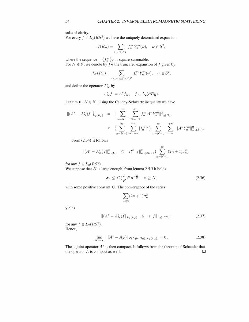
54 CHAPTER 2. INVERSE ELECTROMAGNETIC SCATTERING
sake of clarity.For every f ∈ L2(RS2) we have the uniquely determined expansion
f(Rω) =∑
(n,m)∈I
fmn Y m
n (ω), ω ∈ S2,
where the sequence fmn I is square-summable.
For N ∈ N, we denote by fN the truncated expansion of f given by
fN (Rω) =∑
(n,m)∈I,n≤N
fmn Y m
n (ω), ω ∈ S2,
and define the operator A∗N by
A∗Nf := A∗fN , f ∈ L2(∂BR).
Let ε > 0, N ∈ N. Using the Cauchy-Schwartz inequality we have
‖(A∗ −A∗N )f‖2
L2(Bρ) = ‖∞∑
n=N+1
+n∑m=−n
fmn A∗ Y m
n ‖2L2(Bρ)
≤ (∞∑
n=N+1
+n∑m=−n
|fmn |2 )
∞∑n=N+1
+n∑m=−n
‖A∗ Y mn ‖2
L2(Bρ).
From (2.34) it follows
‖(A∗ −A∗N )f‖2
L2(Ω) ≤ R2 ‖f‖2L2(∂BR) (
∞∑n=N+1
(2n+ 1)σ2n)
for any f ∈ L2(RS2).We suppose that N is large enough, from lemma 2.5.3 it holds
σn ≤ C (ρ
R)n n− 3
2 , n ≥ N, (2.36)
with some positive constant C. The convergence of the series∑n∈N
(2n+ 1)σ2n
yields
‖(A∗ −A∗N )f‖L2(Bρ) ≤ ε‖f‖L2(RS2) (2.37)
for any f ∈ L2(RS2).Hence,
limN→∞
‖(A∗ − A∗N )‖L(L2(∂BR), L2(Bρ)) = 0 . (2.38)
The adjoint operatorA∗ is then compact. It follows from the theorem of Schauder thatthe operatorA is compact as well.

2.5. SPHERICAL SCATTERING OPERATOR 55
Remark. Since the range R(A) of the compact operator A is not closed in L 2(∂BR),the Moore-Penrose or pseudo-inverse operator A † defined for g ∈ D†(A) := R(A)⊕R(A)⊥ by
A†g =∑
(n,m)∈I
σ−1n < g, um
n > vmn
is not bounded. Hence, the problem
Af = g
is ill-posed and regularization techniques are necessary for the inversion, see [Lou89],[Nat01].This issue will be further discussed in chapter 3.
In theorem 2.5.2, the coefficients αn are given as integrals of Bessel functions.To avoid numerical integration of highly oscillating integrands we rather use the firstformula in the following lemma.
Lemma 2.5.4. We have
α2n =
ρ3
2(jn(kρ)2 − jn+1(kρ)jn−1(kρ)
). (2.39)
Furthermore, if kρ = ϑν with ν = (n+ 12 ) and 0 < ϑ < 1, then it holds
α2n ≤ ρ2
4kϑ−2(1 + ϑ2)
12 ν−1e−( 2ν
3 )(1−ϑ2)32 . (2.40)
Proof. From [Luk62] p. 255, we have the identities
ρ∫0
Cν(r)2rdr =ρ2
2(Cν(kρ)2 − Cν+1(kρ)Cν−1(kρ)
), (2.41)
=ρ2
2
((1 − (
ν
kρ)2)Cν(kρ)2 − C
′ν(kρ)
), (2.42)
where Cν is a cylindrical function of order ν and C′ν is its derivative.
The identity (2.39) follows immediately from (2.41) and (B.2).Let ν = (n + 1
2 ), n integer, such that kρ ∈ (ν − 1, ν) and let ϑ = kρν−1. Fromlemma (B.0.2), we have
0 ≤ Jν(νϑ) ≤ (2πν)−12 (1 − ϑ2)−
14 e−( ν
3 )(1−ϑ2)32 ,
0 ≤ ϑJ ′ν(νϑ) ≤ (2πν)−
12 (1 + ϑ2)
14 e−( ν
3 )(1−ϑ2)32 .

56 CHAPTER 2. INVERSE ELECTROMAGNETIC SCATTERING
0 10 20 30 40 50 60 70 800
0.01
0.02
0.03
0.04
0.05
0.06
0.07
0.08
k=10
k=20
k=30
k=50
Figure 2.1: Singular values of of AR,ρ for R = ρ = 1, k ∈ 10, 20, 30, 50.
Thus, using 2.42 we get
α2n =
π
2k
ρ∫0
(Jν(kr))2 rdr
≤ ρ2
8k
(ϑ−2(1 − ϑ2)
12 + ϑ−2(1 + ϑ2)
12
)ν−1e−( 2ν
3 )(1−ϑ2)32
≤ ρ2
8kϑ−2(1 + ϑ2)
12
(1 + (
1 − ϑ2
1 + ϑ2)
12
)ν−1e−( 2ν
3 )(1−ϑ2)32
≤ ρ2
4kϑ−2(1 + ϑ2)
12 ν−1e−( 2ν
3 )(1−ϑ2)32 .
Remark. Asymptotically, the singular values of the spherical scattering operator A
behave like(n− 3
2(
ρR
)n), n → ∞, as we can see from lemma 2.5.3. Nevertheless,
from the estimate in lemma 2.40 we see that there exists a transition region about kρ,where the singular values decay exponentially, see figures (2.1), and (2.2). In otherwords, the singular values of order larger than kρ can be neglected in comparaisonwith those of order smaller than kρ. The spherical scattering operator acts radially as alow-pass filter damping all oscillations related to Bessel functions of order larger thankρ.

2.5. SPHERICAL SCATTERING OPERATOR 57
0 20 40 60 80 1000
0.01
0.02
0.03
0.04
0.05
0.06
0.07
0.08
0.09
0.1
ρ = 4
ρ = 2
ρ = 1
ρ = 0.5
Figure 2.2: Singular values of AR,ρ for k = 15, R = 4, ρ ∈ 0.5, 1, 2, 4.
2.5.2 Null space
The characterization of non-radiating sources is important for solving the inverse sourceproblem. We aim in this subsection to construct a complete orthonormal basis for thenull space of the spherical scattering operator in the three-dimensional case.Within the framework of a boundary value problem for the Helmholtz equation, De-vaney et al [DM98] constructed in 3-D a basis for non-radiating solutions. It is, how-ever, nonorthogonal. In 2-D, Wallacher derived in [Wal02] an orthonormal basis andshowed its completeness using the Lommel theorem for Bessel functions.A powerful tool to derive orthonormal bases is to formulate the problem as a spectraldecomposition of a selfadjoint compact operator.We start with the next lemma, which states that an eigenmode of the Laplace operatorsatisfying some orthogonality relation on the boundary, is either an element of the nullspace N (A) or an element of R(A∗).
Lemma 2.5.5. For λ > 0, λ = k, let φ ∈ C2(Bρ) such that
∆φ = −λ2 φ in Bρ.
Then
φ ∈ N (A) iff
[ ∫∂Bρ
∂nφ v − φ∂n v dσ = 0 for every v ∈ R (A∗)], (2.43)
where ∂n denotes the outward normal derivative to the boundary ∂Bρ.

58 CHAPTER 2. INVERSE ELECTROMAGNETIC SCATTERING
Proof. Since N (A) = R(A∗)⊥, we have
φ ∈ N (A) iff
[ ∫Bρ
φ(x) v(x) dx = 0 for every v ∈ R (A∗)].
From theorem B.0.3 it follows for v ∈ R (A∗) that
v ∈ C2(Bρ ) and (∆ + k2)v = 0.
Hence, the required result follows immediately from the second Green’s formula
−(λ2 − k2)∫Bρ
φ(x) v(x) dx =∫Bρ
∆φ(x) v(x) − φ(x)∆v(x) dx
=∫
∂Bρ
∂nφ(x) v(x) − φ(x) ∂nv(x) dσ(x).
We take now advantage of the spherical symmetry of the problem to make use ofthe method of separation of variables, which leads to the spherical Bessel differentialoperator, see appendix B.
Definition 2.5.6. For n ∈ N, let Ln denote the spherical Bessel differential operatordefined by
Lnf =∂2f
∂r2+
2r
∂f
∂r− n(n+ 1)
r2f for f ∈ C 2(0,∞).
Lemma 2.5.7. Let n ∈ N, αn := jn(kρ), βn := −kj′n(kρ), with jn the sphericalBessel function of order n.Let λ > 0, λ = k. If f = fn, λ ∈ C 2(Bρ ) is a solution to
Lnf = −λ2f,
αn f′(ρ) + βn f(ρ) = 0
, (2.44)
then form ∈ −n, . . . , n, , the function
φmn, λ(x) := fn, λ( |x| )Y m
n (x
|x| ), x ∈ Bρ \ 0, (2.45)
satisfiesφm
n, λ ∈ N (A).
Proof. If φmn, λ,m ∈ −n, · · ·n, , n ∈ N, is given by (2.45), then we have φm
n, λ ∈C 2(Bρ ) and the Laplace operator in polar coordinates reads
∆φmn, λ (x) =
[∂2
∂r2+
2r
∂
∂r+
1r2
∆B
]f(r)Y m
n (ξ)

2.5. SPHERICAL SCATTERING OPERATOR 59
for x ∈ Bρ 0, r = |x| and ξ = x|x| , where ∆B is the Laplace-Beltrami operator.
From (A.7) we obtain∆φm
n, λ = −λ2 φmn, λ.
Let l ∈ N, p ∈ −l, . . . , l, with the notations of theorem 2.5.2 we check for
vpl (x) = γnjn( k |x| )Yn(
x
|x| ), x ∈ Bρ 0,
the orthogonality relation (2.43)∫∂Bρ
[∂n φ
mn, λ (x) vp
l (x) − φmn, λ (x) ∂n v
pl (x)
]dσ(x)
= γn [αn f′n, λ(ρ) + βn fn, λ(ρ) ]
∫S2
Y mn (ξ)Y p
l (ξ) dξ
= γn δnl δmp [αn f′n, λ(ρ) + βn fn, λ(ρ) ] = 0,
where δ denotes the Kronecker symbol.Since vp
l , l ∈ N, p = −l, . . . , l, form a complete orthonormal system in R (A∗), itholds ∫
∂Bρ
[∂n φ
mn, λ (x) v(x) − φm
n, λ (x) ∂n v(x)]dσ(x) = 0
for every v ∈ R(A∗).From the previous lemma we get
φmn, λ ∈ N (A) for n ∈ N, m = −n, . . . , n.
Remark. Lemma 2.5.7 reduces the determination of a basis for the null space N (A)to a Sturm-Liouville problem for the differential operator Ln, which is unfortunatelysingular at zero. The integration of the differential equation for a degenerate Sturm-Liouville problems does not yield a Hilbert-Schmidt integral operator since, due to thesingularity, the corresponding Green’s function is not square integrable on the inter-val (0, ρ), see remarks 16 and 17 p. 51 in [DL90b]. We use the procedure describedtherein to circumvent this difficulty, where we consider the variational formulation,then apply theorem C.0.4. Nevertheless, if we take the whole interval [0, ρ], we haveto investigate the trace properties of the involved Sobolev-spaces, , see [DL90b] p.50.To avoid this task, we proceed indirectly. We first isolate the singularity by consideringthe intervals [ε, ρ], ε > 0, then make ε tend to zero. For the easiness of the reader, wecollect some useful results from [DL90b] in the appendix C.
Without lost of generality we set ρ = 1. Furthermore, an appropriate substitution, see[GR00] 8.49 p. 921, reduces the differential operator Ln to the operator Ln definedby
Lnf = f′′(r) +
(n+
12
)2
r−2 f(r) for f ∈ C2(0,∞).

60 CHAPTER 2. INVERSE ELECTROMAGNETIC SCATTERING
Lemma 2.5.8. Let n ∈ N ∪ 0, (α, β) ∈ R2, β = 0. For every ε > 0, there exists asequence of positive numbers (λ ε
n, k)k ∈N with λ εn, k → ∞, as k → ∞, and a complete
orthonormal system in L2 (ε, 1) of smooth functions (e εn, k)k ∈N satisfying
Ln eεn, k = −λ ε
n, k eεn, k
α∂e ε
n, k
∂r (1) − β e εn, k (1) = 0
e εn, k (ε) = 0
(2.46)
for every k ∈ N.
Proof. LetH = L2 (ε, 1) and V be the closure inH 1(ε, 1) of the space
V := f ∈ C1( [ε, 1] ), f(ε) = 0, α f′(1) − β f(1) = 0 .
In the following chain of inclusions
C∞0 ( [ε, 1] ) ⊂ V ⊂ H1(ε, 1) ⊂ H,
the space C∞0 ( [ε, 1] ) is dense in H and the injection of H 1(ε, 1) into H is compact,
see [Ada75] p. 144.The Hilbert space V is then dense and compactly injected inH .We define on V × V the symmetric bilinear form aε by
aε (f, g) =
1∫ε
f′(r) g
′(r) dr − γ f(1) g(1) + ν
1∫ε
f(r) g(r) r−2 dr, f, g ∈ V,
with
γ =
βα if α = 00 if α = 0
(2.47)
and
ν = (n+12) 2. (2.48)
Lemma C.0.5 implies that aε is continuous and coercive on V × V. We extend aε bydensity on V × V , into a continuous and coercive bilinear form.Furthermore, an integration by parts yields
< −Lnf, g > = −1∫
ε
[ f′′(r) + ν r−2 f(r) ] g(r) dr
=
1∫ε
f′(r) g
′(r) dr − γ f(1) g(1) + ν
1∫ε
f(r) g(r) r−2 dr
= aε (f, g).

2.5. SPHERICAL SCATTERING OPERATOR 61
for every f ∈ C2( [ε, ρ] ) and g ∈ C1( [ε, ρ] ) satisfying the boundary conditions in(2.46).We extend the operator Ln onto the space
D(−Ln) := f ∈ H2(ε, ρ), f(ε) = 0, α f′(1) − β f(1) = 0
such that
< −Lnf, g >= aε (f, g) for every f ∈ D(−Ln), g ∈ V.
From theorem C.0.4, it follows that the spectrum of the self adjoint operator (−L n)defined onD(−Ln) is discrete and admits the positive eigenvalues λ ε
n, kk satisfying
0 < α < λ εn, k, α constant, and lim
k→∞λ ε
n, k = ∞.
More over, the eigenfunctions e εn, k of the operator (−Ln) normalized in H and asso-
ciated with λ εn, k, k ∈ N, built up a complete orthonormal system for H . We further
have e εn, k ∈ C∞( [ε, 1] ) for k ∈ N and the system (2.46) is fulfilled in a classical
sense, see the remark following lemma C.0.5.
We give now an estimate of the eigenvalues λεn,k using the Min-Max formulae
given by theorems C.0.6 and the corollary C.0.7.
Lemma 2.5.9. For ε > 0, k ∈ N, we have( −π2 + k π
1 − ε
)2≤ λ εn, k ≤
[1 + |γ| +
(n+
12)2 ] ( k π
1 − ε
)2.
Proof. For f ∈ C1 ([ε, 1]) with f(ε) = 0, from the Cauchy-Schwartz inequality weget
|f(x)|2 =∣∣ ∫ x
ε
f′(t) dt
∣∣2 ≤ x2
∫ x
ε
|f ′(t)|2 dt, x ∈ [ε, 1].
Hence, for the bilinear form aε we have the estimate∫ 1
ε
|f′(x)|2 dx− |γ| f(1)2 ≤ aε (f, f) ≤
[1 + |γ| +
(n+
12)2 ] ∫ 1
ε
|f′(x)|2 dx
for f ∈ C10 ([ε, 1]), and by density, also for f ∈ H 1
0 (ε, 1).The symmetric bilinear forms b0 and b1 defined by
b0 (f, g) =∫ 1
ε
f′(x) g
′(x) dx, f, g ∈ H1
0 (ε, 1),
and
b1 (f, g) =∫ 1
ε
f′(x) g
′(x) dx − |γ| f(1)2, f, g ∈ H1 (ε, 1),

62 CHAPTER 2. INVERSE ELECTROMAGNETIC SCATTERING
are associated, in the sense of theorem C.0.4, to the Laplace operator (− d2
dx2 ) on [ε, 1],where the Dirichlet boundary conditions (f(1) = f(ε) = 0) lead to b0, and the bound-
ary conditions(f(ε) = 0, f
′(1) = |γ| f(1)
)to b1.
If we apply theorem C.0.6 and corollary C.0.7, we get when we take the right ordering
µεk ≤ λ ε
n k ≤[1 + |γ| +
(n+
12)2 ]
ν εn k, k ∈ N,
where µεk and ν ε
n k are the eigenvalues associated to b1 and b0, respectively. Theseeigenvalues are computed in the remark following lemma C.0.7. Using
ν εn k =
( k π
1 − ε
)2and the estimate ( −π
2 + k π
1 − ε
)2≤ µεk,
we finish the proof of the lemma.
In the next lemma we compute the eigenvalues λεn,k and eigenfunctions eε
n,k givenin lemma 2.5.8.
Lemma 2.5.10. There exist sequences of real numbers (A εn, k) k∈N and (B ε
n, k) k∈N
uniquely determined, such that
e εn, k(x) = x
12[A ε
n, k Jn+ 12
(√λ ε
n, k x) +B εn, k Yn+ 1
2(√λ ε
n, k x)],
where Jn+ 12
and Yn+ 12
are Bessel functions of the first and second kind, respectively.Furthermore, for k ∈ N, we have
limε→0
λ εn, k = λn, k,
where λ12n, kk are positive zeros of the function
ϕn(r) = α r J′
n+ 12(r) − (β − α
2)Jn+ 1
2(r).
When ε tends to zero, we have
limε→0
B εn, k = 0,
limε→0
A εn, k = An, k,
limε→0
e εn, k(x) = en, k(x), x ∈ [0, 1],
where
An, k := 1∫
0
[Jn+ 12(√λn, k r)]2 r dr
− 12 and en, k(x) := An, k x
12 Jn+ 1
2(√λn, k x).

2.5. SPHERICAL SCATTERING OPERATOR 63
Proof. For ε > 0, k ∈ N ∪ 0,λ = λ εn, k, the functions e ε
n, k are solutions to theboundary value problem
y′′(r) + (n+ 1
2 )2 r−2 y(r) = −λ y(r)αy
′(1) − β y(1) = 0
y(ε) = 0,
If we make the substitution y(r) = r12 z (
√λ r), see [GR00] 8.491.5 p. 921, the
differential equation is transformed into the Bessel equation
z′′(t) +
1tz
′(t) +
(1 −
(n+ 12 ) 2
t2)z(t) = 0,
whose fundamental system may be given by the pair Jn+ 12, Yn+ 1
2 of Bessel and
Neumann functions.Hence, there exist uniquely determined constants A ε
n, k and B εn, k such that
e εn, k(r) = r
12[A ε
n, k Jn+ 12
(√λ ε
n, k r) +B εn, k Yn+ 1
2(√λ ε
n, k r)]
with
α e εn, k
′(1) − β e ε
n, k(1) = 0
and
e εn, k(ε) = 0.
From lemma 2.5.9 we havelimε→0
ε√λ ε
n, k = 0
Since the Neumann function Yn+ 12
is singular at 0, we must have
limε→0
B εn, k = 0
and
limε→0
A εn, k =
1∫0
[Jn+ 12(√λn, k r)]2 r dr
− 12 ,
to fulfill the boundary condition at ε and the normalizing condition ‖e εn, k‖ = 1.
Finally, the boundary condition at 1 implies, when ε tends to zero, that λ n, k have tosatisfy
ϕn (√λn, k) = 0.
Remarks.
1. The positive zeros of the function ϕn are simple and may be ascendingly ar-ranged in a sequence (λn, k)k∈N, see also [Wat58] p. 480.

64 CHAPTER 2. INVERSE ELECTROMAGNETIC SCATTERING
2. We have for k ∈ N ∪ 0 the identity
A−2n, k =
12
[J
′n+ 1
2(√λn, k)
] 2if α = 0
12 λn,k
[ (β−α2 )2
α2 + λn, k − (n+ 12 )2
]Jn+ 1
2(√λn, k)2 otherwise,
see [AS72] 11.4.5 p. 485.
3. In the sequel we use also the notations λ 0n, k := λn, k, e 0
n, k := en, k.
Bearing in mind that we seek the limiting case as ε tends to zero, we need to look intothe convergence of eε
n,k in L2(0, 1).
Lemma 2.5.11. If we extend e εn, k by zero outside (ε, 1), ε > 0, then the functions
e εn, k are uniformly bounded, in ε, on the interval (0, 1) and they converge to en, k inL2(0, 1).
Proof. Let n ∈ N ∪ 0, k ∈ N and A be a constant with |A εn, k| ≤ A for ε ≥ 0.
The Bessel function of the first kind Jn+ 12
is bounded by 1 on [0,∞) and the Besselfunction of the second kind Yn+ 1
2is singular at zero and bounded away from zero, see
[AS72] p. 362.We have for ε small enough
|Yn+ 12
(x) | ≤ |Yn+ 12
(ε) |, x ∈ (ε,∞).
We recall thatlimε→0
ε√λ ε
n, k = 0.
Let ε > 0 be small enough, from the boundary condition at ε in (2.46) it holds
B εn, k Yn+ 1
2(ε√λ ε
n, k) = −A εn, k Jn+ 1
2(ε√λ ε
n, k).
We obtain for x ∈ (ε, 1) the estimate
e εn, k(x) := x
12[A ε
n, k Jn+ 12
(√λ ε
n, k x) +B εn, k Yn+ 1
2(√λ ε
n, k x)]
≤ x12[|A ε
n, k Jn+ 12
(√λ ε
n, k x) | + |A εn, k Jn+ 1
2(√λ ε
n, k ε) |]
≤ 2A
which proves that the extended e εn, k are uniformly bounded on (0, 1) for ε ≥ 0.
We can therefore, interchange the limit and the integration to get
limε→0
1∫0
| (e εn, k − en, k)(x) |2 dx = 0
The convergence in L2(0, 1) is proved.

2.5. SPHERICAL SCATTERING OPERATOR 65
Theorem 2.5.12. The system en, kk∈ N is orthonormal and complete in L2(0, 1).
Proof. The system en, kk ∈N is orthogonal since for k, l ∈ N we have
−(λn, k − λn, l ) < en, k, en, l >=< Ln en, k, en, l > − < en, k, Ln en, l >= 0.
To prove completeness, we construct first the ”inverse” operator K of (−Ln). Wedefine the operatorKε ∈ L
(L2(0, 1)
), ε > 0, by
Kεf(x) =
∑∞k=0
1λ ε
n, k< f, e ε
n, k > e εn, k(x), x ∈ (ε, 1),
0 x ∈ [0, ε].
For ε > 0, the operatorKε is compact, as a limit of finite rank operators, and we have
‖Kε‖ =1
λ εn, 1
.
From lemma 2.5.9 , we see that Kε are uniformly bounded for ε > 0, it follows fromthe Banach-Steinhaus theorem of uniformboundedness thatK ε converge inL
(L2(0, 1)
),
as ε tends to zero, to an operatorK ∈ L(L2(0, 1)
).
The operatorK is compact and it is given by
Kf = limε→0
Kεf, f ∈ L2(0, 1). (2.49)
From lemma 2.5.11 it follows
K f(x) =∞∑
k=0
1λn, k
< f, en, k > en, k(x), x ∈ (0, 1).
Let f ∈ C20 (0, 1) and ε0 such that the support of f is contained in [ε0, 1 − ε0] and
0 < ε < ε0. Integrating by parts we get
< Ln f, eεn, k >=< f,Ln e
εn, k >= −λ ε
n, k < f, e εn, k > for everyk ∈ N.
It yields
−KεLn f =∞∑
k=0
< f, e εn, k > e ε
n, k = f.
The last equality holds, since (e εn, k)k form a complete orthonormal system in L2(ε, 1)
and vanishes outside (ε, 1). Hence, when ε tends to zero, we get
−K Ln f = f for every f ∈ C20 (0, 1).
The expansion
f(x) =∞∑
k=0
< f, en, k > en, k(x), x ∈ (0, 1),
holds also for f ∈ L2(0, 1) since C20 (0, 1) is dense in L2(0, 1).
The completeness of en, kk∈N in L2 (0, 1) has been also proved.

66 CHAPTER 2. INVERSE ELECTROMAGNETIC SCATTERING
Remark. When α = 0, theorem 2.5.12 is known as the Fourier-Bessel expansion,which can also be proved using the Lommel theorem for Bessel functions, see [Hoc86].The advantage of using the techniques from [DL90b] is that the proof only relies ontheorem C.0.4.In general, boundary conditions are part of the features of Sturm-Liouville problems,which explains the complications related to the case when α = 0.
We come back now to the system fn,kk constructed in lemma 2.5.7 and showits completeness in L2(0, ρ, r2dr).
Corollary 2.5.13. Let n ∈ N, αn := jn(kρ), βn := −kj′n(kρ) = 0. Let λn,k be thepositive zeros of
αn λj′n(λρ) + βn jn(λρ) = 0. (2.50)
Then the system fn,kk, fn,k(r) := an,kjn(λn,kr), r ∈ (0, ρ), built up a completeorthonormal system of L2(0, ρ, r2dr), where an,k are normalizing coefficients.
Proof. Let ρ = 1. As en,k(r) =(
π2
)− 12 An,kλ
12n,k rjn(λn,kr), k ∈ N, from theorem
2.5.12 build up a complete orthonormal system of L 2(0, 1) for each fixed n ∈ N, thefunctions r−1en,k(r)k form also a complete orthonormal system of (L2(0, 1), r2dr).Hence, the corollary follows from the previous theorem with the right choice of (α, β).
We can use the bases fn,kk from the corollary above and spherical harmonicsto construct a complete orthonormal basis of N (A) building up with vm
n (n,m) acomplete orthonormal system of L2(Bρ).
Theorem 2.5.14. Let n ∈ N.Form ∈ −n, . . . , n, let
φmn, k(x) := fn, k( |x| )Y m
n (x
|x| ), x ∈ Bρ \ 0. (2.51)
Then φn,kmk built up a complete orthonormal system of N (A).
Remark. We see from (2.50), that the null space N (A) obviously depends on theradius of the target region ρ, however, it does not depend on the radius R of themeasurement sphere. Therefore, if we have an apriori information about the locationof the scatterer, we can use ρ as a parameter to control the zeros related to the radialpart of the elements of the basis of N (A).
2.5.3 Sobolev estimate
We close this section with a result about the smoothing properties of the spherical scat-tering operator in the setting of Sobolev-spaces. As we will see in the next chapterthe inverse scattering problem is solved approximately using a regularization method.The smoothing properties of the underlying operator account for the accuracy of thecomputed solution , see [Lou89] , [Nat01].

2.5. SPHERICAL SCATTERING OPERATOR 67
In this subsection we use on the Sobolev-space H s(Rn), s ∈ R, the equivalent norm 3
‖f‖Hs(Rn) =
∫Rn
(1 + |ξ|2)s|f(ξ)|2dξ
12
, f ∈ Hs(Rn),
where the Fourier transform f of f is defined by
f(ξ) = (2π)−n2
∫Rn
f(t)e−i<ξ,t>dt.
Let Ω be a bounded domain in Rn. For s ∈ R, we put
Hs0(Ω) := f ∈ Hs(Rn), f is compactly supported in Ω.
Let χ be the characteristic function of Ω, we define the norm
‖f‖Hs(Ω) = ‖χf‖Hs(Rn).
Lemma 2.5.15. Let k > 0 and R > 0. The Fourier transform of the function gk,R
defined on R3 by
gk,R(x) :=
14π
eik|x||x| if |x| < R
0 if |x| ≥ R
is given by
gk,R(ξ) = −(|ξ|2−k2)−1
(1 − eikR(cos(R|ξ|) − ik
sin(R|ξ|)|ξ|
)for ξ ∈ R3\0.
Proof. For ξ ∈ R3, we have
gk,R(ξ) = (2π)−32
∫R3
gk,R(x)e−i<ξ,x>dx
= (2π)−32
∫BR
gk(x)e−i<ξ,x>dx for ξ ∈ R3.
Let φξ(x) := e−i<ξ,x>, x ∈ R3. As (∆ + k2)φξ = (k2 − |ξ|2)φξ, we get
gk,R(ξ) = (k2 − |ξ|2)−1
∫BR
gk(x)(∆ + k2)φξ(x)dx for |ξ| = k.
3see [Nat01] p. 201 or [DL88] p.96.

68 CHAPTER 2. INVERSE ELECTROMAGNETIC SCATTERING
Let ε > 0, Br be the ball centered at the origin with radius r ∈ ε,R .From the second Green’s formula, we have∫BR\Bε
gk(x)(∆ + k2)φξ(x)dx =∫
BR\Bε
(∆ + k2)gk(x)φξ(x)dx
+∫
∂BR
(gk(x)∂nφξ(x) − ∂ngk(x)φξ(x)) dσ(x)
−∫
∂Bε
(gk(x)∂nφξ(x) − ∂ngk(x)φξ(x)) dσ(x),
where ∂n denotes the outward normal derivative.The first integral on the right-hand side vanishes since gk is the Green’s function for∆ + k2 . It remains only to compute the boundary integrals.From the Funk-Hecke theorem it follows, on the one hand,∫
∂Br
φξ(x)dσ(x) = r2∫S2
e−ir<ξ,ω>dω
= 2πr21∫
−1
e−ir|ξ|tdt
= 4πrsin(r|ξ|)
|ξ| ,
on the other hand,∫∂Br
∂nφξ(x)dσ(x) = −ir2∫S2
< ξ, ω > e−ir<ξ,ω>dω
= −2iπ|ξ|r21∫
−1
te−ir|ξ|tdt
= 4πr(
cos(r|ξ|) − sin(r|ξ|)r|ξ|
).
As g′k(r) =(ik − 1
r
)gk(r) with r ∈ ε,R, we obtain after a straightforward com-
putation
limε→0
∫∂Bε
∂ngk(x)φξ(x)dσ(x) = −1 and limε→0
∫∂Bε
gk(x)∂nφξ(x) = 0,
and ∫∂BR
gk(x)∂nφξ(x) − ∂ngk(x)dσ(x) = eikR
(cos(R|ξ|) − ik
sin(R|ξ|)|ξ|
).

2.5. SPHERICAL SCATTERING OPERATOR 69
Lemma 2.5.16. There exists a constant m > 0 such that
|gk,R(ξ)| ≥ m max(|ξ|, k)−1 (|ξ| + k)−1.
Proof. We write
|gn,k(ξ)| = (|ξ| + k)−1
∣∣∣∣eikR q(|ξ|) − q(k)|ξ| − k
∣∣∣∣with
q(t) := cos(Rt) − iksin(Rt)
t, t > 0.
Since the continuous function q(t)− q(k) only vanishes at the simple zero t = k, weget ∣∣∣∣q(|ξ|) − q(k)
|ξ| − k
∣∣∣∣ ≥ mmax(|ξ|, k)−1,
for some constant m > 0.
Remark. Contrary to gk, we see from the proof above that gR,k has no singularity at|ξ| = k.
Lemma 2.5.17. Let s ≥ 0, a > 0. There is a constant C > 0 such that
sup|ξ|≤a
|f(ξ)| ≤ C ‖f‖Hs0(Ω)
for f ∈ C∞0 (Ω).
The proof of the lemma can be found in [Nat01] p.44. It is also to mention thatsome techniques used in the proof of the next theorem are inspired from the samereference.
Theorem 2.5.18. Let s ≥ 0 and AΩ : Hs0(Ω) −→ L2(Ω) be the scalar scattering
operator. Then there exist two positive constants c(s) and C(s) such that we have
c(s) ||f ||Hs0 (Ω) ≤ ||AΩf ||Hs+2(Ω) ≤ C(s) ||f ||Hs
0 (Ω) (2.52)
for every f ∈ C∞0 (Ω).
Proof. First of all, we notice that it holds
AΩf(x) = χ(x)∫
Bρ
gk(x− y)f(y)dy =∫Bρ
gk,R(x − y)f(y)dy for x ∈ Bρ,

70 CHAPTER 2. INVERSE ELECTROMAGNETIC SCATTERING
with R = 2ρ, since |x− y| < 2ρ for x, y ∈ Bρ.Let s ≥ 0 and f ∈ C∞
0 (Ω). We have
‖AΩf‖2Hs+2(Ω) =
∫R3
(1 + |ξ|2)s+2|χAΩf(ξ)|2dξ (2.53)
= (2π)3∫R3
(1 + |ξ|2)s+2|f(ξ)|2|gk,R(ξ)|2dξ (2.54)
≥ (2π)3m2
∫R3
(1 + |ξ|2)s|f(ξ)|2(
1 + |ξ|2max(|ξ|, k)(|ξ| + k)
)2
dξ
≥ (2π)3 min(12,
12k2
)2m2 ‖f‖2Hs
0(Ω),
by virtue of the convolution theorem for the Fourier transform and lemma 2.5.16.To prove the inequality on the right-hand side, we split the integration domain in (2.54)into ξ, |ξ| ≤ a and ξ, |ξ| ≥ a, where we take a > max(k, 1) such that
|ξ|2|ξ|2 − k2
≤√
2 for |ξ| ≥ a. (2.55)
On the one hand, from lemma 2.5.17 we have
∫|ξ|≤a
(1 + |ξ|2)s+2|f(ξ)|2|gk,R(ξ)|2dξ ≤ sup|ξ|≤a
|f(ξ)|2∫
|ξ|≤a
|gk,R(ξ)|2(1 + |ξ|2)s+2dξ
≤ C2(s)‖f‖2Hs
0(Ω)
with some constant C2(s) > 0, since the last integral is finite.On the other hand, it holds
|gk,R(ξ)| ≤ (2 + kR)||ξ|2 − k2|−1,
where we dominated cos(R|ξ|) and sin(R|ξ|)R|ξ| by 1. Using (2.55) we get∫
|ξ|≥a
(1 + |ξ|2)s+2|f(ξ)|2|gk,R(ξ)|2dξ ≤ 2(2 + kR)2∫
|ξ|≥a
ϕ(ξ)2(1 + |ξ|2)s|f(ξ)|2dξ
≤ 23(2 + kR)2∫
|ξ|≥a
(1 + |ξ|2)s|f(ξ)|2dξ
≤ 23(2 + kR)2‖f‖2Hs
0(Ω),
where ϕ(ξ) := |ξ|−2(1 + |ξ|2) ≤ 2 for |ξ| ≥ 1.The proof is then finished.

2.5. SPHERICAL SCATTERING OPERATOR 71
Corollary 2.5.19. Let Ω = Bρ ⊂ R3 be the ball centered at the origin with radiusρ > 0, s ≥ 0 and AΓ : Hs
0(Ω) −→ L2(Γ) be the restricted scattering operator onthe boundary Γ := ∂Bρ. Then there exist two positive constants c(s) and C(s) suchthat we have
c(s) ||f ||Hs0 (Ω) ≤ ||AΓf ||
Hs+ 32 (Ω)
≤ C(s) ||f ||Hs0 (Ω) (2.56)
for every f ∈ C∞0 (Ω) .
Proof. If we write AΓ = γ0AΩ with the trace mapping γ0 on the boundary Γ. Thecorollary follows from theorem 2.5.18 and theorem D.0.9.
The singular value decomposition, the determination of the null space and the studyof the smoothing properties for the spherical scattering operator in three-dimensionprovide us good tools to deal with the regularization of the inverse problem in the nextchapter.

72 CHAPTER 2. INVERSE ELECTROMAGNETIC SCATTERING

Chapter 3
Application of the approximateinverse
The problem (A,X, Y ) of solving the equation Af = g for a bounded linear opera-tor A between the Hilbert spaces X and Y is well-posed according to Hadamard iffor any data g ∈ Y there exists a solution f , this solution is unique, and it is stablethrough perturbation of the right-hand side, in a sense that the solution f ε for the datagε is closer to f, the closer gε is to g . It is well known that if A is compact and itsrange is not closed, the problem (A,X, Y ) is in this case rather ill-posed. Since forsuch an operator the Moore-Penrose or pseudo-inverse A † is unbounded, the conditionof stability is violated. Typically, data are endowed with noise, which is an unavoidableerror generally related to measurement conditions.The application of a regularization method is then required to stabilize the solution. Itconsists in approximating the ill-posed problem by a class of neighboring well-posedproblems. In [Lou99], it has been shown that regularization methods can be consideredwhether as smoothing of the pseudo-inverse or as prewhitening of the data. Regular-ization algorithms of broad usage such as Thikhonov-Phillips, the truncated singularvalue decomposition, iterative Landweber or conjugate gradient can be considered asfiltered version of the pseudo-inverse. Alternatively, mollifier methods consist in com-puting smoothed versions of the solutions, see [Lou99] and the references therein.The approximate inverse, introduced for linear problems presents a unified approach toregularization methods for linear ill-posed problems. It is also extendible to some non-linear problems, see [Lou96]. Efficient algorithms based on the approximate inversehas been generated for many applications. Recent applications of the approximate in-verse can be found in [Sch00] and [AS04] for 3-D tomography, in [DRT00] for localtomography, in [HSS05] for thermo-acoustic computed tomography.The first application of the approximate inverse to backscattering problems is due toAbbdullah and Louis [Abd98]. Their scheme for 2-D acoustic waves is derived fromthe Lippmann-Schwinger integral equation, where a linear inversion with the approx-imate inverse provides the equivalent source. Wallacher in [Wal02] improved the res-olution of the nonlinear part in that scheme to recover the medium properties from the
73

74 CHAPTER 3. APPLICATION OF THE APPROXIMATE INVERSE
equivalent source. He also extended the scope of application to limited-angel problems.
3.1 The approximate inverse
In this section we recall some fundamental properties of the approximate inverse as aregularization method and describe how to realize an efficient implementation usingthe invariances of the problem. Three features characterize this method
1. Stability and robustness, due to the precomputation of the reconstruction kernelindependently from data.
2. Efficiency, by using the invariance properties of the problem to compute thereconstruction kernel. Once the kernel is is on hand, any new data can be rapidlyinverted.
3. Flexibility in the choice of the filter appropriately to the problem.
3.1.1 Regularization with the approximate inverse
Definition 3.1.1. Let A be a compact operator between the Hilbert spaces X and Y,A† be its pseudo-inverse. A regularization Tγγ>0 of A† is a family of continuousoperators Tγ : Y −→ X such that there exists a mappingγ : R+ × Y −→ R+, called a regularizing parameter, satisfying
limε→0
Tγ(ε,gε)gε = A†g
for every g ∈ D(A†) := R(A) ⊕R(A)⊥ and gε ∈ Y with ‖g − gε‖ ≤ ε.If Tγ are all linear, then Tγγ>0 is called linear regularization.
Let n,m ∈ N, Ω ⊂ Rn and Γ ⊂ Rm be measurable sets, the spaces X ⊂L2(Ω)N , Y ⊂ L2(Γ)M and Z ⊂ L2(Γ)P , M,N, P ∈ N, be Hilbert spaces.
Definition 3.1.2. The operators Mγγ>0 ⊂ L(X) form an approximation of theidentity if
limγ→0
Mγ f = f for f ∈ X.
We say that it has the rate α > 0 if there exists a positive constant C > 0 such that
‖Mγf − f‖ ≤ Cγα ‖f‖ for f ∈ X. (3.1)
If furthermore for x ∈ Ω, there exists exγ ∈ X such that for f ∈ X
Mγ f(x) =< f, exγ >, x ∈ Ω,
then the function eγ defined by
eγ(x, y) := exγ(y) for x, y ∈ Ω,
is called the mollifier associated to Mγ .

3.1. THE APPROXIMATE INVERSE 75
Definition 3.1.3. Let A ∈ L(X,Y ), eγ be a mollifier and D : X → Z be a linearoperator on the subspace X ⊂ X.If we assume that for every x ∈ Ω, there exists a minimum-norm solutionψx
γ ∈ R(A) to the equationA∗ψx
γ = D∗exγ , (3.2)
then we call the operator Sγ : Y → Z defined for g ∈ Y by
Sγ g(x) =< g, ψxγ >, x ∈ Ω, (3.3)
the approximate inverse and the function ψγ defined by
ψγ(x, y) = ψxγ (y), x ∈ Ω, y ∈ Γ,
the reconstruction kernel, to compute the moment D of the solution.
Lemma 3.1.4. We suppose that Γ is bounded. For the operator A : X → Y and themollifier eγ , let Sγ be the approximate inverse to compute the moment D : X → Z.If, for every γ > 0, the mollifier ex
γ satisfies supx∈Ω
‖D∗exγ‖ <∞ andD∗ex
γ ∈ R(A∗), x ∈Ω, then
limγ→0
Sγ Af = Df for f ∈ N (A)⊥.
Proof. Let γ > 0. For x ∈ Ω, the equation
A∗ψxγ = D∗ex
γ
admits a unique minimum-norm solution ψ xγ ∈ R(A), see [Lou89].
Let g ∈ R(A) and f ∈ N (A)⊥ be a solution to Af = g. Then for x ∈ Ω, we have
Sγ g(x) =< Af, ψxγ >=< f,A∗ψx
γ >=< f,D∗exγ >=< D f, ex
γ > .
From the Cauchy-Schwartz inequality we get
|Sγ g(x)| = | < f,D∗exγ > | ≤ ‖D∗ex
γ‖ ‖f‖.
As Γ is assumed to be bounded with measure |Γ|, it yields
‖Sγg‖ ≤ |Γ| supx∈Ω
‖D∗exγ‖ ‖f‖.
Hence Sγg ∈ L2(Ω)P .Since ex
γ is associated to an approximation of the identity, we have
limγ→0
Sγ Af = Df.

76 CHAPTER 3. APPLICATION OF THE APPROXIMATE INVERSE
Remarks
1. The adjoint equation (3.2) is independent of the right hand side g. The recon-struction kernel ψγ is precomputed independently from errors related to mea-sured data. This yields a stable reconstruction of Df .
2. The operator D gives the moment of the solution f we ought to compute. Forinstance, an averaged version of f is computed by taking D the identity onX = Z . To compute other moments Df of the solution, we simply ”transpose”the operator D on the mollifier. This generalizes the procedure already used byLouis in [Lou96] to compute the derivative of the solution. Schuster in [Sch00]applied also this technique to compute the curl of the solution for the Doppler-transform in 3-D tomography. We may similarly extend this method to solveill-posed equations, where the gradient, divergence or curl of the solution is re-quired. The inversion is then carried in a stable way, without any differentiationof the measured data.
Examples. For the sake of simplicity, let D be the identity on X and M = N =P = 1. A mollifier eγ is said to be of convolution type if
eγ(x, y) = γ−n e0(x− y
γ), γ > 0, x, y ∈ Rn,
for some function e0 ∈ L2(Rn) with∫Rn
e0(x) dx = 1.
The last condition is set to ensure that constant functions are invariant under mollifica-tion.For example, to compute local averages of the solution, we may take
e0(x) =n
|Sn−1| χ(x),
where χ is the characteristic function of the unit ball of Rn and |Sn−1| is the measureof the surface in the unit ball in Rn.The band-limited filter
e0(x) = π−n sinc (x),
is used to eliminate the high-frequency component of the solution.The Gauss-function is a very smoothing mollifier. It is given by
e0(x) = (2π)−n2 exp (−|x| 2
2).
In lemma 3.1.4, the required conditions on the mollifier are overdoing. They maybe improved if the smoothing properties of the operator A are involved. For this

3.1. THE APPROXIMATE INVERSE 77
purpose we consider an appropriate space setting, we refer to [Lou89], [Lou99] formore details.Let X and Y be two Hilbert spaces, A : X −→ Y be a non degenerate compactoperator with singular system vn, un;σnn∈N. For ν ∈ R, the spaces
Xν :=
f ∈ N (A)⊥,
∑n∈N
σ−2νn | < f, vn > |2 <∞
endowed with the scalar product
< f, g >:=∑n∈N
σ−2νn < f, vn >< g, vn >
and the norm
‖f‖Xν :=
(∑n∈N
σ−2νn | < f, vn > |2
) 12
built up a pre-Hilbert scale Xνν∈R .
Definition 3.1.5. Let X and Y be two Hilbert spaces, A : X −→ Y be a nondegenerate compact operator with singular system vn, un;σnn∈N.
1. The problem (A,X, Y ) is said to be ill-posed with the order α > 0 if σn =O(n−α).If furthermore, f ∈ Xν with ν = β
α , β > 0, is solution to the equation Af =g, g ∈ R(A), we say the problem is ill-posed of order (α, β).
2. The problem (A,X, Y ) is said to be exponentially ill-posed if there exist positiveconstants and C such that | log(σn)| ≥ Cn.
The ill-posedness is measured by the number α, the a priori information aboutthe solution is given by the number ν. The spaces Xνν build up a Hilbert-scale tomeasure the smoothness of the solution, see [Lou99]. The next lemma, see [Lou89]p.50, shows the connection of this concept of smoothness with the classical Sobolev-spaces.
Lemma 3.1.6. Let Ω ⊂ Rn be open, A : L2(Ω) −→ L2(Ω) be a compact operatorwith singular system vn, un;σnn∈N. If
‖f‖L2(Ω) ≤ ‖Af‖Hα(Ω) ≤ ‖f‖L2(Ω), (3.4)
then there exist positive constants c1 and c2 such that
c1σn ≤ ‖vn‖Hα(Ω) ≤ c2σn and c1σn ≤ ‖un‖Hα(Ω) ≤ c2σn, n ∈ N. (3.5)
Lemma 3.1.7. Let Mγ : X−1 −→ X be a family of linear bounded operators suchthat
1. ||Mγf || ≤ cαγ−α||Af || for all f ∈ N (A)⊥,

78 CHAPTER 3. APPLICATION OF THE APPROXIMATE INVERSE
2. ||Mγf − f || ≤ cβγβ‖f‖ for all f ∈ N (A)⊥,
with α > 0, β > 0. Iflim
γ,ε→0εγ−α = 0,
then Tγ := MγA† is a linear regularization of A† for finding f, where the operatorA† : Y −→ X−1 denotes the extension by density of A† on Y.Furthermore, if Af = g, f ∈ N (A)⊥, g, gε ∈ Y, with
‖g − gε‖ ≤ ε and ‖f‖Xν ≤ ,
where ν := βα , then there exists a regularizing parameter γ = γ(ε, , α, ν) and a
constant C > 0 such that
‖Tγgε − f‖ ≤ Cε
νν+1
1ν+1 .
Proof. See [Lou99].
In other words, the regularization is conditioned by the quality of the mollifier forsmoothing and approximating. The approximation M γ of the identity must be at leastof the same smoothing order as the operator A.
3.1.2 Invariance properties
To apply the method of the approximate inverse for solving the equation
Af = g,
we use the solutions to the adjoint equations
A∗ψxγ = ex
γ for every x ∈ Ω.
As the adjoint equations are independent of the measured data, the inversion algorithmis stable. Nevertheless, the gain in stability has apparently its price, since we have todeal with an operator equation of higher order. Indeed, if A is an integral operatorwith kernel k, then the corresponding adjoint equations can be reduced to determine akernel ψγ , solution to∫
Γ
ψγ(x, z) k(z, y)dz = eγ(x, y), x, y ∈ Ω.
However, if the operator A has invariance properties, which is the case in most appli-cations, we do not need to directly solve the adjoint equations for every x ∈ Ω.
Lemma 3.1.8. Let A ∈ L(X,Y ). For x ∈ Ω, let the operators T x1 ∈ L(X) and
T x2 ∈ L(Y ) satisfy
T x1 A
∗ = A∗T x2 and T x
3 A = AT x1 .

3.2. REGULARIZATION OF THE SCATTERING OPERATOR 79
Further, let exγ = eγ(x, ·), γ > 0, be a mollifier satisfying
exγ = T x
1 Eγ with Eγ ∈ D((A∗)†).
If φγ is a solution ofAA∗φγ = AEγ , (3.6)
then the solution ψxγ of
AA∗ψxγ = Aex
γ
is given byψx
γ = T x2 φγ . (3.7)
If we further have Eγ ∈ R(A∗), then the solution ψxγ of
A∗ψxγ = ex
γ
is given byψx
γ = T x2 φγ , (3.8)
where φγ is the solution ofA∗φγ = Eγ . (3.9)
The usage of invariance properties reduces dramatically the effort of computationand storage. We have only to solve the adjoint equation (3.6) or (3.9) for few recon-struction points, then deduce the reconstruction kernel ψ x
γ for every x ∈ Ω from (3.8)or (3.7). The evaluation of the solution with the precomputed reconstruction kernelrequires only a matrix vector multiplication. This makes inversion schemes based onthe approximate inverse very efficient.
3.2 Regularization of the scattering operator
We want now to apply the results of the previous section to regularize the sphericalscattering operator using the method of the approximate inverse. As we mentioned be-fore, the smoothing properties of the operator and its order of ill-posedness are closelyrelated to each other.
Theorem 3.2.1. Let 0 < ρ ≤ R and A : X → Y be the spherical scattering operatorwith X = L2(Bρ) and Y = L2(∂BR).
1. If ρ = R, the problem (A,X, Y ) is ill-posed of order 32 .
2. If ρ < R, the problem (A,X, Y ) is exponentially ill-posed.
Proof. This result follows immediately from definition 3.1.5 and lemma 2.5.3.
Remarks.

80 CHAPTER 3. APPLICATION OF THE APPROXIMATE INVERSE
1. We can see from corollary 2.5.19 that the order of ill-posedness of the problem(A,X, Y ) for the spherical scattering operator A with ρ = R, agrees with itsorder of smoothing on the Sobolev-scale, which is also equal to 3
2 .Despite the apparent mildness of the problem (A,X, Y ) when ρ = R, it cre-ates, when kρ is small, as much difficulty as severely ill-posed problems. Def-inition 3.1.5 relates the ill-posedness to the asymptotic behavior of the singularvalues for large order, however the fast decay of the singular values of the spher-ical scattering operator begins earlier at the orders close to kρ, as we can seefrom the remark following lemma 2.5.4. This behavior is comparable to the situ-ation met in computer-tomography for the limited-angle problem for the Radontransform, see [Lou86] and [Nat01] p. 160.
2. The localization of the target domain, by taking ρ smaller, enhances the ill-posedness of the inverse problem.
Corollary 3.2.2. The norm ‖ · ‖1 on the space X1 for the restricted scattering oper-ator A with ρ = R, is equivalent to the Sobolev-norm ‖ · ‖
H32 (Ω)
.
Proof. This directly follows from the theorem above, lemma 3.1.6 and corollary 2.5.19.
We look now into the invariance properties of the spherical scattering operator.
Lemma 3.2.3. LetA ∈ L(L2(Bρ), L2(∂BR)), 0 < ρ ≤ R, be the spherical scatteringoperator and U be a rotation about the origin of R3.On the spacesX1 = L2(Bρ), X2 = L2(BR), we define the operatorsTU
i ∈ L(Xi), i ∈ 1, 2, by
TUi f = f U for f ∈ Xi, i = 1, 2.
Then we have
TU1 A
∗ = A∗TU2 , (3.10)
A TU1 = TU
2 A. (3.11)
Proof. We prove only (3.10), the identity (3.11) can be proved similarly.Let ϕ ∈ X2, x ∈ Bρ. We have
TU1 A
∗ϕ(x) = A∗ϕ(Ux)
=∫
∂BR
gk(|Ux− y|)ϕ(y) dσ(y)
=∫
∂BR
gk(|x− U∗y|)ϕ(y) dσ(y)
=∫
∂BR
gk(|x− t|)ϕ(Ut) dσ(t)
= A∗TU2 ϕ(x),

3.2. REGULARIZATION OF THE SCATTERING OPERATOR 81
where we used the substitution y = Ut and the fact that U is orthogonal and preserves∂BR invariant.
Although, the spherical scattering operator is not invariant under translation, theeffort to compute its reconstruction kernel may be significantly reduced. The previouslemma incites us to consider mollifiers of the form
eγ(x, y) = e0γ(x− y), x, y ∈ R3,
with e0γ is invariant under rotation.
Theorem 3.2.4. For γ > 0, let eγ(x, y) = eγ(|x − y|), x, y ∈ R3, be a mollifiersatisfying ex
γ := eγ(x, ·) ∈ R(A∗) ⊕ R(A)⊥ for every x ∈ Bρ. With the notationof theorem 2.5.2, the reconstruction kernel for the spherical scattering operator A isgiven by
ψγ(x, y) =∞∑
n=0
n∑m=−n
σ−1n wγ
n,m(x)un,m(y), x ∈ Bρ \ 0, y ∈ ∂BR, (3.12)
where the functions wγn,m for m = −n, · · · , n, n ∈ N, are defined by
wγn,m = φγ
n(|x|)Y mn (
x
|x| ) for x ∈ Bρ \ 0, (3.13)
with
φγn(u) := 2πγn
ρ∫0
1∫−1
r2jn(kr)eγ((u2 + r2 − 2rut)12 )Pn(t)dtdr, u > 0, (3.14)
where Pn is the Legendre Polynomial of order n.
Proof. Let γ > 0, x ∈ Bρ. Using the singular value system of the operator A, theminimum-norm solution of the equation
A∗ψxγ = ex
γ
gives the reconstruction kernel ψxγ at the point x as an expansion
ψxγ =
∑n∈N
n∑m=−n
σ−1n < ex
γ , vn,m >L2(Bρ) un,m, (3.15)
where the convergence holds in L2(∂BR) for exγ ∈ R(A∗) ⊕R(A∗)⊥.
Let x = uθ with u > 0, θ ∈ S2. Form = −n, · · · , n, n ∈ N, we have
< exγ , vn,m > =
∫Bρ
eγ(|x− y|)vn,m(y)dy
= γn
ρ∫0
r2jn(kr)
∫S2
eγ
((u2 + r2 − 2ur < θ, ω >)
12
)Y m
n (ω) dω
dr

82 CHAPTER 3. APPLICATION OF THE APPROXIMATE INVERSE
From the Funk-Hecke theorem we get∫S2
eγ
((u2 + r2 − 2ur < θ, ω >)
12
)Y m
n (ω)dω = Iγn(u, r)Y m
n (θ)
with
Iγn(u, r) = 2π
1∫−1
eγ
((u2 + r2 − 2urt)
12
)Pn(t)dt,
where Pn is the Legendre polynomial.
The invariance under rotation of the spherical scattering operator reduces the com-putation of the convolution < ex
γ , vn,m > to the evaluation of the integral I γn , which
is cheaper in terms of computational effort. We can further simplify the computationof the kernel as we can see from the following result.
Corollary 3.2.5. We maintain the notations of the theorem above. The reconstructionkernel for the spherical scattering operator A satisfies
ψγ(x, y) =∞∑
n=0
2n+ 14πR
σ−1n φγ
n(|x|)Pn(x · y|x||y| ), x ∈ Bρ \ 0, y ∈ ∂BR. (3.16)
Proof. The result follows immediately from theorem 3.2.4 and the identity A.13.
Remark. If x0 ∈ S2 is fixed e.g. x0 := (0, 0, 1), the reconstruction kernel forx ∈ Bρ \ 0, y ∈ ∂BR, satisfies
ψγ(x, y) = ψγ(rx0, tx0), with r = |x|, t|t| = r−1R−1x · y. (3.17)
This means that we have only to compute the reconstruction kernel at the reconstructionpoints (rx0, tx0) then use (3.17).
Theorem 3.2.6. If eγ(x) = e0γ(x− y), x, y ∈ R3, γ > 0, is a mollifier satisfying
1. e0γ ∈ H32 (R3) with ‖e0γ‖H
32 (R3)
≤ cαγ−α,
2. ||(2π)32 e0γ − 1||∞ ≤ cβγ
β ,
where cα, cβ > 0, α, β > 0, are constants, then the approximate inverse Sγ definedby (3.12) is a regularization for the pseudo-inverse A† of the restricted scatteringoperator A with ρ = R.Furthermore, let g, gε ∈ Y and Af = g with f ∈ N (A)⊥. If
‖g − gε‖ ≤ ε and ‖f‖Xν ≤
where ε, are positive constants and ν := βα , then there exists a regularizing param-
eter γ = γ(ε, , α, ν) such that
‖Sγgε − f‖ ≤ Cε
νν+1
1ν+1 (3.18)
with some constant C > 0.

3.2. REGULARIZATION OF THE SCATTERING OPERATOR 83
Proof. To prove theorem 3.2.6 we apply lemma 3.1.7.Let Mγ be the smoothing operator defined for f ∈ L2(R3) byMγf(x) :=< f, ex
γ > . Let f ∈ N (A)⊥ given by the expansion
f =∞∑
n=0
n∑m=−n
fmn v
mn ,
with respect to the singular functions vmn n,m of A.We have
||Mγf ||2 =∫
BR
| < f, exγ > |2dx
=∫
BR
|∞∑
n=0
n∑m=−n
fmn < vm
n , exγ > |2dx
≤( ∞∑
n=0
n∑m=−n
σ2n|fm
n |2)∫
BR
∞∑n=0
n∑m=−n
| < σ−1n vm
n , exγ > |2dx
.
≤ ‖f‖2X−1
∫BR
‖exγ‖2
X1dx
From corollary 3.2.2 there exists a constant c > 0 such that
‖exγ‖X1 ≤ c‖ex
γ‖H32.
Since exγ(ξ) = ei<ξ,x>e0γ(ξ), we have
‖exγ‖H
32
= ‖e0γ‖H32.
For f ∈ N (A)⊥ we get
‖Mγf‖ ≤ c vol(BR)12 ‖f‖X−1‖e0γ‖H
32
≤ Cγ−α‖f‖X−1,
where vol(BR) denotes the volume of BR and C := c cα vol(BR)12 . The first con-
dition in lemma 3.1.7 is then proved.By virtue of the Parseval identity and the convolution theorem for the Fourier trans-form, we obtain
||Mγf − f ||2 ≤∫
R3
∣∣∣∣∫R3e0γ(x − y)f(y)dy − f(x)
∣∣∣∣2 dx≤
∫R3
|((2π)32 e0γ(ξ) − 1)f(ξ)|2 dξ
≤ ||(2π)32 e0γ(ξ) − 1)||2∞
∫R3
|f(ξ)|2 dξ
≤ (cβγβ)2||f ||2,

84 CHAPTER 3. APPLICATION OF THE APPROXIMATE INVERSE
0
0.5
1
−1
−0.5
0
0.5
1−1000
−500
0
500
1000
−800
−600
−400
−200
0
200
400
600
800
Figure 3.1: The real part of the reconstruction kernel for k = 15, γ = 0.05,R = ρ = 1.
which proves the second condition in lemma 3.1.7 and finishes the proof of the theorem.
Remark. In the figures 3.1-3.4 we give for the spherical scattering operator A ρ,R,plots of the reconstruction kernel computed for the Gauss-mollifier, where φ γ
n is eval-uated numerically.
3.3 Resolution of the inverse source problem
We consider a spherical geometry with the ball Ω = Bρ as a target region and thesphere Γ = ∂BR as a measurement surface, 0 < ρ ≤ R.Let AΓ = Aρ,R be the spherical scattering operator and AΩ be the scalar scatteringoperator.For N ∈ 3, 6, the measurement operator MΓ is defined by
MΓg := (γ0gj)j ,g = (gj)j∈1,··· ,N ∈ H1(Ω)N ,
where γ0 is the trace mapping on the boundary Γ.We denote by AΩ and AΓ the operators defined by
AΩf := (AΩfj)j , f = (fj)j∈1···N ∈ L2(Ω)N ,
andAΓf := (AΓfj)j , f = (fj)j∈1···N ∈ L2(Ω)N ,
respectively. To simplify the notations, we may denote AΩ and AΓ both by A, anddenote AΩ and AΓ by A.

3.3. RESOLUTION OF THE INVERSE SOURCE PROBLEM 85
0
0.5
1
−1
−0.5
0
0.5
1−3000
−2000
−1000
0
1000
−2500
−2000
−1500
−1000
−500
0
500
Figure 3.2: The imaginary part of the reconstruction kernel for k = 15, γ = 0.05,R = ρ = 1.
0
0.5
1
−1
−0.5
0
0.5
1−1000
−500
0
500
1000
−400
−200
0
200
400
600
Figure 3.3: The real part of the reconstruction kernel for k = 15, γ = 0.05,R = 1, ρ = 0.5.

86 CHAPTER 3. APPLICATION OF THE APPROXIMATE INVERSE
0
0.5
1
−1
−0.5
0
0.5
1−1500
−1000
−500
0
500
1000
−1200
−1000
−800
−600
−400
−200
0
200
400
600
Figure 3.4: The imaginary part of the reconstruction kernel for k = 15, γ = 0.05,R = 1, ρ = 0.5.
3.3.1 The nonmagnetic case
We consider the inverse source problem for a nonmagnetic medium.Given d = (dj)j=1,2,3. ∈ L2(Ω)3, determine q ∈ H2
0 (Ω)3 such that
MΓTeq = d, (3.19)
whereTe = k2A − Kd
is the nonmagnetic scattering operator.We may write
Te = k2A − A′ div,
where A′ is the second scattering operator.The equation (3.19) reads then
k2Aq(x) − (A′ div q)(x) = d(x), x ∈ Γ. (3.20)
By virtue of theorem 2.4.4 we have
Te = AP, (3.21)
where the nonmagnetic scattering potential P is given by
Pq = k2q + grad(div q).
Our inverse source problem can thus be reformulated as the following systemAΓw=dP q=w . (3.22)

3.3. RESOLUTION OF THE INVERSE SOURCE PROBLEM 87
We utilize the approximate inverse Sγ of A†Γ for some smooth mollifier eγ to com-
pute an approximation to the generalized induced source w γ = (wjγ)j , γ > 0, ob-
tained bywj
γ = Sγdj , j ∈ 1, 2, 3, (3.23)
which is the regularized solution of the first equation in (3.22).When we replace w by the smoother approximation wγ in the second equation of(3.22), we get using theorem 2.4.5
div qγ = −Adivwγ . (3.24)
The evaluation of vγ := −Adivwγ determines an approximation to div q, whichwe insert in the second term of the left-hand side of (3.20). Hence, we can approximateA′ div q in (3.20) by computing
cγ = A′vγ . (3.25)
The problem is reduced to solve the equation
AΓq = gγ (3.26)
with the new right-hand side gγ = (gjγ)j=1,2,3. given by
gγ = k−2(d + cγ). (3.27)
To solve the equation (3.26), we apply again the approximate inverse. We finally re-cover the source qγ = (qj
γ)j=1,2,3. from
qjγ = Sγg
jγ , j ∈ 1, 2, 3. (3.28)
Remarks.
1. Since the operator A is of convolution type we can use FFT techniques, see[Nat01] p. 207, to compute vγ . The evaluation of cγ = A′vγ is only needed onΓ. Besides, the resolution of the inverse source problem involves the applicationof the approximate inverse twice and the computation of the divergence in (3.24).All these computations can be carried efficiently with a low cost in terms ofstorage and computational effort.
2. The differentiation in (3.24) to compute the divw γ is not problematic providedwe choose a smooth mollifier eγ . An alternative way to proceed is to carrythe differentiation on the mollifier itself. This approach will be treated for thegeneral case of electromagnetic media.
3.3.2 The electromagnetic case
We consider now the inverse source problem for an electromagnetic medium.Given d = (dj)j=1,··· ,6 ∈ L2(Ω)6, determine f ∈ H2
0 (Ω)6 such that
MΓTemf = d, (3.29)

88 CHAPTER 3. APPLICATION OF THE APPROXIMATE INVERSE
where Tem is the electromagnetic scattering operator.We denote V the first electromagnetic scattering potential and W the second electro-magnetic scattering potential.
Let X = (L2(Ω))6 and Y = (L2(Γ))6. We define a bilinear form on X × X by
((f ,g))X = (< fi, gi >)i=1,··· ,6, for f = (fj)j ,g = (gj)j ∈ X
and a bilinear form on Y × Y by
((f ,g))Y = (< fi, gi >)i=1,··· ,6, for f = (fj)j ,g = (gj)j ∈ Y.
We may in the sequel abusively denote ((·, ·))X and ((·, ·))Y both by ((·, ·)).
Definition 3.3.1. Let Exγ = (Ex
γ,j)j ∈ L2(Ω)6, γ > 0, be a mollifier and
Exγ(y) = −WAΩ Ex
γ(y) (3.30)
with respect to x, for y fixed. The function kγ : Ω × Γ −→ C6,kγ = (kγ,j)j ,defined by
kγ,j(x, y) =∞∑
n=0
n∑m=−n
σ−1n um
n (y) < Exγ,j, v
mn >, j ∈ 1 · · · 6, (3.31)
is called the reconstruction kernel, and the operator Sγ defined for g ∈ (L2(Γ))6 by
Sγg(x) = ((g,kγ(x, ·))), x ∈ Ω,
is called the approximate inverse, for the electromagnetic inverse source problem.
Remark. The idea of using a modified version of the approximate inverse based on thebilinear forms ((·, ·))X and ((·, ·))X , instead of the scalar products of the underlyingvector field spaces, had been already applied by Schuster to vector tomography, see[Sch00] for more details.
In the sequel, the mollifier is assumed to be smooth enough to justify the underlyinginterchanges of integration and differentiation and to permit the passages to the limit.
Lemma 3.3.2. For a smooth mollifier Exγ = (Ex
γ,j)j=1,··· ,6, γ > 0, let Sγ be thecorresponding approximate inverse for the electromagnetic inverse source problem.Then
Sγg(x) = ((Exγ ,A
†Γg)), g = (gj)j ∈ L2(Γ)6, x ∈ Ω, (3.32)
where Exγ(y) = −WAΩ Ex
γ(y) with respect to x, for y fixed.
Proof. For j ∈ 1, · · · , 6, g = (gj)j ∈ L2(Γ)6, we have
(Sγg)j := < gj, kγ,j >
=∞∑
n=0
n∑m=−n
σ−1n < gj , u
mn >< Ex
γ,j, vmn >
= < Exγ,j,A
†Γg >,
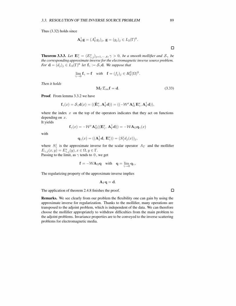
3.3. RESOLUTION OF THE INVERSE SOURCE PROBLEM 89
Thus (3.32) holds since
A†Γg = (A†
Γgj)j , g = (gj)j ∈ L2(Γ)6.
Theorem 3.3.3. Let Exγ = (Ex
γ,j)j=1,··· ,6, γ > 0, be a smooth mollifier and Sγ bethe corresponding approximate inverse for the electromagnetic inverse source problem.For d = (dj)j ∈ L2(Γ)6 let fγ := Sγd. We suppose that
limγ→0
fγ = f with f = (fj)j ∈ H20 (Ω)6.
Then it holdsMΓTemf = d. (3.33)
Proof. From lemma 3.3.2 we have
fγ(x) = Sγd(x) = ((Exγ ,A
†Γd)) = ((−WxAx
Ω Exγ ,A
†Γd)),
where the index x on the top of the operators indicates that they act on functionsdepending on x.It yields
fγ(x) = −WxAxΩ((Ex
γ , A†Γd)) = −WAΩqγ(x)
withqγ(x) = ((A†
Γd, Exγ)) = (Sj
γdj(x))j ,
where Sjγ is the approximate inverse for the scalar operator AΓ and the mollifier
Eγ,j(x, y) = Exγ,j(y), x ∈ Ω, y ∈ Γ.
Passing to the limit, as γ tends to 0 , we get
f = −WAΩq with q = limγ→0
qγ ,
The regularizing property of the approximate inverse implies
AΓq = d.
The application of theorem 2.4.8 finishes the proof.
Remarks. We see clearly from our problem the flexibility one can gain by using theapproximate inverse for regularization. Thanks to the mollifier, many operations aretransposed to the adjoint problem, which is independent of the data. We can thereforechoose the mollifier appropriately to withdraw difficulties from the main problem tothe adjoint problems. Invariance properties are to be conveyed to the inverse scatteringproblems for electromagnetic media.

90 CHAPTER 3. APPLICATION OF THE APPROXIMATE INVERSE
3.4 Resolution of the inverse medium problem
We describe now an iterative procedure to reconstruct the contrast function from dataof multiple experiments using the generalized induced source formulation for the in-verse scattering problem.
Let X and Y be two Hilbert spaces, V be a subspace of X, the bilinear operatorQ : V ×X −→ X define the product Q(f, u) = fu of f ∈ V and u ∈ X. Let Vbe an open subset of V . For f ∈ V, we denote Qf ∈ L(X) the operator defined byQfu := Q(f, u), u ∈ X.We consider T ∈ L(X) such that for f ∈ V the operators (I+TQf) and (I+QfT )are bounded and invertible with (I+TQf)−1 and (I+QfT )−1 as inverse operators,respectively.The nonlinear Lippmann-Schwinger operator A : V × X −→ X for the scatteringoperator T is, therefore, well-defined and satisfies
A(f, u0) = (I + TQf)−1u0, f ∈ V, u0 ∈ X. (3.34)
We further suppose that there exist A ∈ L(X) and U ∈ L(X) such that
T = AU, (3.35)
where U is invertible with inverse U−1.For the j−th experiment, j ∈ I := 1, · · · , p, p ∈ N, let u0
j ∈ X denote the incidentfield.We assume, for the sake of simplicity, that we have the same measurement operatorMΓ ∈ L(X,Y ) for all experiments.We denote AΓ := MΓA and suppose that Sγγ>0 is a regularization for the ill-posedproblem (AΓ, X, Y ).
Definition 3.4.1. We define the (nonlinear) source operator φ : V × X −→ X forf ∈ V, u0
j ∈ X byφ(f, u0
j) = fu with u = A(f, u0j). (3.36)
We denote φj(f) := φ(f, u0j ) and φ′
j(f) its Frechet-derivative.Further, we define the nonlinear operator Fj : V −→ Y for f ∈ V by
Fj(f) = MΓTφj(f). (3.37)
We denote F ′j the Frechet-derivative of Fj and F the opeartor
F (f) = (F1(f), · · · , Fp(f))T . (3.38)
For the datad = (d1, · · · , dp) ∈ Y p,
the inverse medium problem can be formulated as a least-square problem:
F (f) = d. (3.39)

3.4. RESOLUTION OF THE INVERSE MEDIUM PROBLEM 91
The application of the Gauss-Newton method to solve (3.39) requires the inversionof the operator (F ′
j(f)∗F ′k(f))−1
j,k=1,··· ,p at each Newton-iteration. For most applica-tions, this challenging computational effort makes the implementation unfeasible withstandard computers.To overcome this difficulty, one approach is to modify the Jacobian operator usingsome approximation. However, the costs for storage and computation remains a realdefiance. In the framework of electromagnetic inversion we refer, about this approach,to the works of Newmann et al [NH00],[NB04] and Haber [Hab04].Alternatively, we use the method applied by Natterer and Wubelling for ultrasoundtomography [NW95],[NW01], by Dorn et al. [DBABC99],[DBABP02] and also byVogeler [Voe03] for electromagnetic imaging. The quasi-Newton method of Gutmannand Klibanov [GK93],[GK94]. uses also a similar approach.The idea is to solve in each step only the linearized equation
Fj(f) + F ′j(f)hj = dj . (3.40)
The minimal norm solution of (3.40) is given by
hj = −F ′j(f)∗C−1
j (Fj(f) − dj) with Cj = Fj(f)F ′j(f)∗. (3.41)
In each step an approximation f 0 is incremented, using some relaxation factor w ∈(0, 2), into a new approximation f 1 as follows
1. f0 = f0
2. For j = 1, · · · , p :
fj = fj−1 + whj with hj = −F ′j(fj−1)C−1
j (Fj(fj−1) − dj) (3.42)
3. f 1 = fp.
This is the extension to nonlinear problems of the Kaczmarz method or algebraic recon-struction technique (ART) of computerized tomography for solving under-determinedlinear systems, see [Nat01] and [NW01].The computational effort to evaluate C−1
j is, however, still too demanding. In [NW95],[DBABC99],[DBABP02],[Voe03], the operator Cj , is replaced by an easy to computeand invert matrix, namely a constant factor times the identity.To avoid such an empirical consideration, we proceed differently to solve the equation(3.42), where we make use of the equivalent source formulation.
Theorem 3.4.2. Let j ∈ I, dj ∈ D(A†Γ), f ∈ V. We suppose that for γ > 0 there
exists hγj ∈ R(F ′
j(f)∗) such that
φ′j(f)hγj = U−1Sγdj − φj(f). (3.43)
Then hγj tends to hj, as γ tends to 0, with
hj = −F ′j(f)∗
(F ′
j(f)F ′j(f)∗
)−1 (Fj(f) − dj).

92 CHAPTER 3. APPLICATION OF THE APPROXIMATE INVERSE
Proof. For hγj ∈ R(F ′
j(f)∗) we have
hγj = F ′
j(f)∗(F ′j(f)∗)†hγ
j = F ′j(f)∗
(F ′
j(f)F ′j(f)∗
)−1F ′
j(f)hγj .
As F ′j(f) = MΓAUφ
′j(f) = AΓUφ
′j(f), we get using (3.35) and (3.37)
hγj = F ′
j(f)∗(F ′
j(f)F ′j(f)∗
)−1AΓUφ
′j(f)hγ
j
= F ′j(f)∗
(F ′
j(f)F ′j(f)∗
)−1AΓU
(U−1Sγdj − φj(f)
)= F ′
j(f)∗(F ′
j(f)F ′j(f)∗
)−1(AΓSγdj − Fj(f))
Since Sγ is a regularization for AΓ, AΓSγdj tends to dj , as γ tends to 0, andconsequently
limγ→0
hγj = hj . (3.44)
Lemma 3.4.3. Let f ∈ V . The Frechet-derivative φ′j(f) ∈ L(X) of the source
operator φj(f) for some incident field u0j ∈ X is given by
φ′j(f)h = (I +QfT )−1h(I + TQf)−1u0j , h ∈ V . (3.45)
Proof. Let f ∈ V. The source operator φj(f) for some incident field u0j ∈ X is
defined byφj(f) = fu with u = u0
j − Tfu.
If we multiply both sides of the last equation by f we obtain
φj(f) = fu0j − fTφj(f). (3.46)
It yieldsφ′j(f)h = hu0
j − fTφ′j(f)h− hTφj(f), h ∈ V . (3.47)
That is
(I +QfT )(φ′j(f)h) = hu with u = A(f, u0j) = (I + TQf)−1u0
j . (3.48)
Remarks.
1. At each iteration, we need to solve for given f the forward problem
uj = (I + TQf)−1u0j
just once, from which we deduce φj(f) = fuj.Let denote
qγj := U−1Sγdj − φj(f). (3.49)
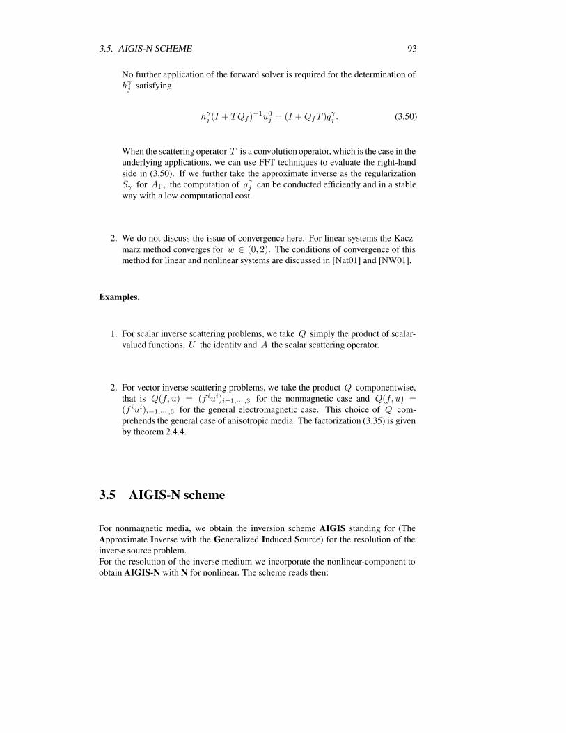
3.5. AIGIS-N SCHEME 93
No further application of the forward solver is required for the determination ofhγ
j satisfying
hγj (I + TQf)−1u0
j = (I +QfT )qγj . (3.50)
When the scattering operator T is a convolution operator, which is the case in theunderlying applications, we can use FFT techniques to evaluate the right-handside in (3.50). If we further take the approximate inverse as the regularizationSγ for AΓ, the computation of qγ
j can be conducted efficiently and in a stableway with a low computational cost.
2. We do not discuss the issue of convergence here. For linear systems the Kacz-marz method converges for w ∈ (0, 2). The conditions of convergence of thismethod for linear and nonlinear systems are discussed in [Nat01] and [NW01].
Examples.
1. For scalar inverse scattering problems, we take Q simply the product of scalar-valued functions, U the identity and A the scalar scattering operator.
2. For vector inverse scattering problems, we take the product Q componentwise,that is Q(f, u) = (f iui)i=1,··· ,3 for the nonmagnetic case and Q(f, u) =(f iui)i=1,··· ,6 for the general electromagnetic case. This choice of Q com-prehends the general case of anisotropic media. The factorization (3.35) is givenby theorem 2.4.4.
3.5 AIGIS-N scheme
For nonmagnetic media, we obtain the inversion scheme AIGIS standing for (TheApproximate Inverse with the Generalized Induced Source) for the resolution of theinverse source problem.For the resolution of the inverse medium we incorporate the nonlinear-component toobtain AIGIS-N with N for nonlinear. The scheme reads then:

94 CHAPTER 3. APPLICATION OF THE APPROXIMATE INVERSE
AIGIS-N
PrecomputationGiven a mollifier eγ ,compute the reconstruction kernel ψγ
for the approximate inverse Sγ .
Input:For each experiment j ∈ I = 1, · · · , p we have:
• Incident electrical fields Eincj (x), x ∈ Ω.
• Scattered electrical fields dj(x) ∈ C3, x ∈ Γ.
Linear inversionFor each experiment j ∈ I = 1, · · · , p :
1. Compute the generalized induced source w jγ = (Sγd
ji )i=1,2,3.
2. Compute vjγ div qj : vj
γ = −Adivwjγ
3. Compute cjγ = A′ vj
γ
4. Compute gjγ = k−2(dj + cj
γ)
5. Compute the equivalent source qj = (Sγ gjγ,i)i
Nonlinear iterationsGiven:Relaxation parameter: wInitial guess: f 0
Maximal number of iterations: N
For n = 1, · · · , N :
1. f0 = fn−1
2. For j = 1, · · · , p :
(a) Ej = (I + Te fj−1)−1Eincj
(b) hγj : hγ
j E0j = (I + fj−1 Te)(q
γj − fj−1 Ej)
(c) fj = fj−1 + w hγj
3. fn = fp.

Chapter 4
Numerical results
To numerically test the AIGIS-N scheme for the resolution of the inverse source andinverse medium problems, we consider two objects with simple geometry, namely asphere and a cylinder. This choice is motivated by the availability of an analyticalsolution for the forward scattering problem. The dimension and the electromagneticproperties of the buried objects are taken close to realistic values for some medical ap-plications of microwave-tomography, see [SBS+00]. The scatterers are nonmagneticwith electrical contrasts beyond the Born/Rytov approximation, according to the con-dition (15) in [KS88] p. 214 .
Reconstruction for the MIE-Model
For our first numerical experiment, we use the analytical solution of the Mie scatteringproblem. It concerns the electromagnetic scattering of a monochromatic plane wave,linearly polarized, by a homogeneous ball with radius r, constant electrical permettiv-ity ε and electrical conductivity σ, which is immersed in a homogeneous nonconduct-ing medium with constant electric permittivity ε0 and magnetic permeability µ0.We take a cartesian system of coordinates (ex, ey, ez) with the origin at the center ofthe sphere. The incident electrical field is polarized in the x−direction and the wave ispropagating in the z−direction, that is
Einc(x) = exp(ikz) ex
with the angular frequency 1 ω, and the wavenumber k = w√ε0µ0.
We assume that the scatterer is non-magnetic and has the refractive index 2
n = ε−10 (ε+ i
σ
ω) (4.1)
with the dielectric permittivity ε and electric conductivity σ. The contrast function is
f = (1 − n)χ, (4.2)
1The frequency is given by ν = w2π
.2In [BW99], the refractive index is alternatively defined by n = (ε−1
0 (ε + i 4πσω
))12 .
95

96 CHAPTER 4. NUMERICAL RESULTS
where χ is the characteristic function of the ball centered at the origine with radius r.The Mie or also called Debye formulae provide the analytical solution to time-harmonicMaxwell equations. They are derived using spherical coordinates by matching bound-ary conditions to determine transmission coefficients, see (57)-(62) in [BW99] p.772and also [Kon90] p.493. We use these formulae to simulate the scattered field outsidethe scatterer.
For the numerical experiment we make the following considerations:
1. Incident electrical field:
(a) Plane wave propagating in the z-direction.
(b) Monochromatic wave with wavenumber k = 30m−1 corresponding tothe frequency ν 1.43GHz.
(c) Linearly polarized in x−direction.
2. Scatterer:
(a) Homogeneous spherical sphere centered at the origin with radius r = 20 cm.
(b) Non-magnetic medium with the electrical contrast function f = 48 + 14i.
3. Experimental setting:
(a) The measurement set Γ is a sphere centered at the origine with radiusR = 1.
(b) The target domain is a ball centered at the origine with radius ρ = 1.
(c) Data are the simulated complex-valued scattered electrical field E s(x), x ∈Γ.
(d) Noisy data are endowed with a normally distributed random error of 10%.
4. Discretization
(a) The computational domain is a cube [−1, 1]3.
(b) The number of grid points in each direction is 64.
5. The mollifier is the Gauss function.
In figures 4.1-22, we give 1-D, 2-D and 3-D representations of the reconstructed complex-valued equivalent source fE.Reconstructions from noisy data with a random error of 10% are presented in figures4.19-4.22.From the obtained results, we can make the following observations:
1. The location is coarsely determined. Dominant oscilliations announce the cross-ing of the boundary. This can be clearly seen for the component parallel to thedirection of polarisation, as well as the transversal component, of the reconstruc-tion.

97
2. An estimate of the contrast is given by the amplitude of the dominant oscillia-tions for the component parallel to the polarization.
3. The shape is clear, however, this may be also due to the spherical symmetry ofthe problem.
4. Almost no information is contained in the component of the equivalent sourceparallel to the direction of propagation.
5. With noisy data we see that the linear inversion is stable.

98 CHAPTER 4. NUMERICAL RESULTS
10 20 30 40 50 60
10
20
30
40
50
60−40
−30
−20
−10
0
10
20
30
40
50
60
Figure 4.1: The real part of the x−component of the recovered equivalent source in thezy−plane through the origin.
−1 −0.5 0 0.5 1−50
0
50
100
−1 −0.5 0 0.5 1−40
−20
0
20
40
60
Figure 4.2: The crossing-plot along the axes of the figure above

99
10 20 30 40 50 60
10
20
30
40
50
60−20
−10
0
10
20
30
40
Figure 4.3: The real part of the x−component of the recovered equivalent source in theyx−plane through the origin.
−1 −0.5 0 0.5 1−50
0
50
100
−1 −0.5 0 0.5 1−40
−20
0
20
40
60
Figure 4.4: The crossing-plot along the axes of the figure above

100 CHAPTER 4. NUMERICAL RESULTS
10 20 30 40 50 60
10
20
30
40
50
60−12
−10
−8
−6
−4
−2
0
2
4
6
8
Figure 4.5: The imaginary part of the x−component of the recovered equivalent sourcein the zy−plane through the origin.
−1 −0.5 0 0.5 1−15
−10
−5
0
5
10
−1 −0.5 0 0.5 1−10
−5
0
5
10
Figure 4.6: The crossing-plots along the axes of the figure above

101
10 20 30 40 50 60
10
20
30
40
50
60 −0.8
−0.6
−0.4
−0.2
0
0.2
0.4
0.6
0.8
Figure 4.7: The imaginary part of the y−component of the recovered equivalent sourcein the yx−plane through the origin.
−1 −0.5 0 0.5 1−0.1
0
0.1
0.2
0.3
−1 −0.5 0 0.5 1−1
−0.5
0
0.5
1
Figure 4.8: The crossing-plots along the axes of the figure above

102 CHAPTER 4. NUMERICAL RESULTS
10 20 30 40 50 60
10
20
30
40
50
60 −2
−1.5
−1
−0.5
0
0.5
1
Figure 4.9: The real part of the y−component of the recovered equivalent source in thezy−plane through the origin.
−1 −0.5 0 0.5 1−0.15
−0.1
−0.05
0
0.05
−1 −0.5 0 0.5 1−0.4
−0.2
0
0.2
0.4
0.6
Figure 4.10: The crossing-plot along the axes of the figure above

103
10 20 30 40 50 60
10
20
30
40
50
60 −0.4
−0.3
−0.2
−0.1
0
0.1
0.2
0.3
0.4
Figure 4.11: The real part of the y−component of the recovered equivalent source inthe yx−plane through the origin.
−1 −0.5 0 0.5 1−0.15
−0.1
−0.05
0
0.05
−1 −0.5 0 0.5 1−0.4
−0.2
0
0.2
0.4
0.6
Figure 4.12: The crossing-plot along the axes of the figure above

104 CHAPTER 4. NUMERICAL RESULTS
10 20 30 40 50 60
10
20
30
40
50
60
−3
−2
−1
0
1
2
3
4
Figure 4.13: The imaginary part of the y−component of the recovered equivalentsource in the zy−plane through the origin.
−1 −0.5 0 0.5 1−0.1
0
0.1
0.2
0.3
−1 −0.5 0 0.5 1−1
−0.5
0
0.5
1
Figure 4.14: The crossing-plots along the axes of the figure above

105
−1−0.5
00.5
1
−1
−0.5
0
0.5
1−1
−0.5
0
0.5
1
−30
−20
−10
0
10
20
30
40
50
Figure 4.15: Real part of the x-component of the computed equivalent current source.
−1−0.5
00.5
1
−1
−0.5
0
0.5
1−1
−0.5
0
0.5
1
−10
−8
−6
−4
−2
0
2
4
6
Figure 4.16: Imaginary part of the x-component of the computed equivalent currentsource .

106 CHAPTER 4. NUMERICAL RESULTS
−1−0.5
00.5
1
−1
−0.5
0
0.5
1−1
−0.5
0
0.5
1
−1.5
−1
−0.5
0
0.5
1
1.5
Figure 4.17: Real part of the y-component of the computed equivalent current source.
−1−0.5
00.5
1
−1
−0.5
0
0.5
1−1
−0.5
0
0.5
1
−3
−2
−1
0
1
2
3
Figure 4.18: Imaginary part of the y-component of the computed equivalent currentsource .

107
10 20 30 40 50 60
10
20
30
40
50
60 −40
−20
0
20
40
60
Figure 4.19: The real part of the x− component of the equivalent source in the zy−plane through the origin recovered from noisy data at a level of 10%.
10 20 30 40 50 60
10
20
30
40
50
60
−2.5
−2
−1.5
−1
−0.5
0
0.5
1
1.5
Figure 4.20: The real part of the y− component of the equivalent source in the zy−plane through the origin recovered from noisy data at a level of 10%.
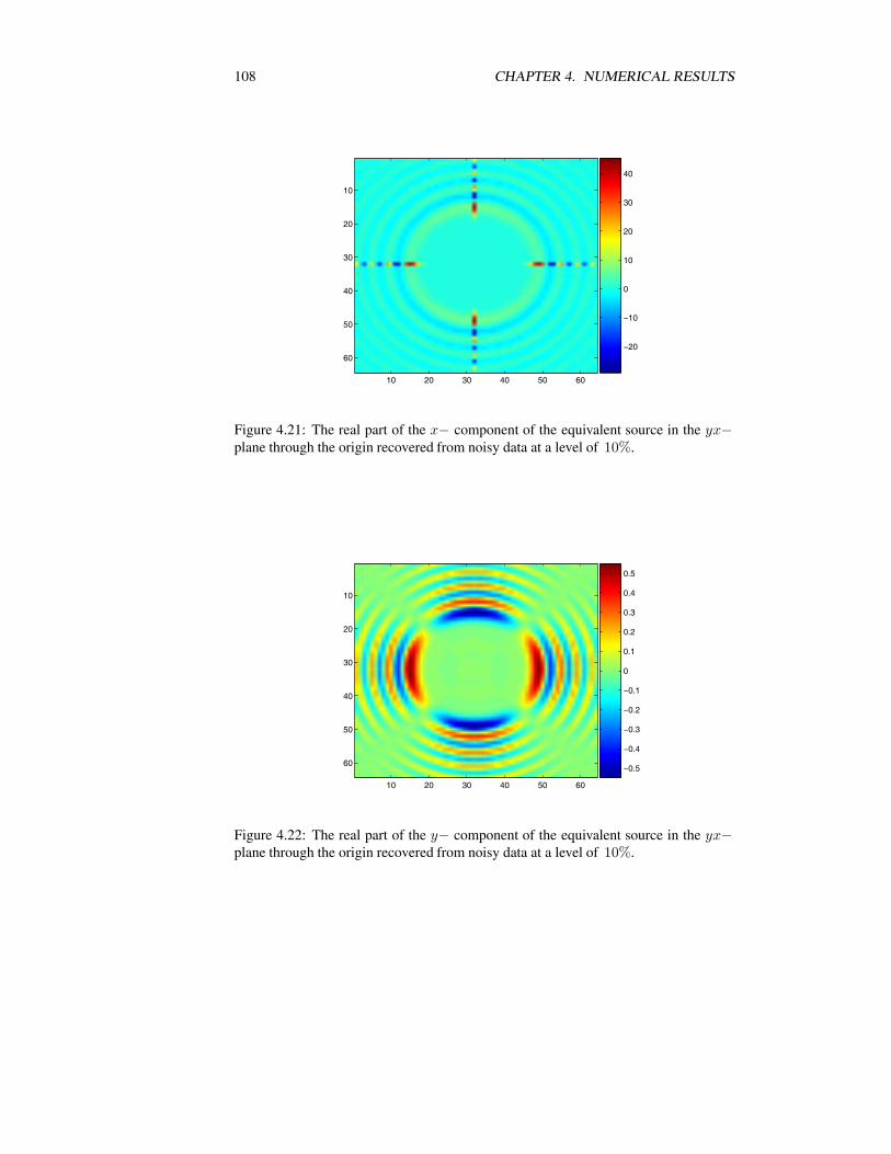
108 CHAPTER 4. NUMERICAL RESULTS
10 20 30 40 50 60
10
20
30
40
50
60−20
−10
0
10
20
30
40
Figure 4.21: The real part of the x− component of the equivalent source in the yx−plane through the origin recovered from noisy data at a level of 10%.
10 20 30 40 50 60
10
20
30
40
50
60−0.5
−0.4
−0.3
−0.2
−0.1
0
0.1
0.2
0.3
0.4
0.5
Figure 4.22: The real part of the y− component of the equivalent source in the yx−plane through the origin recovered from noisy data at a level of 10%.

109
Nonlinear reconstruction for a homogeneous cylinder
To test the nonlinear reconstruction, we take as scatterer a homogeneous cylinder. Theanalytical solution is also obtained by matching the boundary conditions, see for ex-ample [Kon90] p. 497.
1. Incident electrical field properties:
(a) Plane wave propagating in each of the directions dα ∈ S2, such thatdα = dα(α, 0) in cylindrical coordinates.
(b) Monochromatic wave at the frequency ν 4GHz.(c) Linearly polarized in z−direction.
2. Scatterer properties:
(a) Homogeneous cylinder parallel to the polarization direction z and passingthrough the point (0,−0.25, 0). It has the axial-length L = 1m and thecross-section with the radius ρ = 25 cm.
(b) Dielectric medium with real-valued contrast function f = 3.
3. Experimental setting:
(a) The measurement set Γ is a sphere centered at the origin with radius R =1m.
(b) The target domain is a ball centered at origin with radius ρ = R.
(c) Data are the the simulated complexe-valued scattered electrical field E sα(x),
x ∈ Γ for each direction α = 2πm ,m = 0, · · · ,M − 1,M = 36.
4. The mollifier is the Gauss function.
For each direction dα, we make the linear inversion to recover the equivalent sourceqα = (qα
j )j .The main difficulty we face to implement the nonlinear scheme is to incorporate a re-liable forward solver for the vector integral equations modeling the direct problem.One would think to formulate these equations in convolution form, and use FFT tech-niques to solve them. Unfortunately, this approach involves hypersingular kernels,which cause the run-away of the resolution. Hence, the development of a forwardsolver is not immediate and would timely escape out of the objectives of this work.Commercial programs generally use the formulation as partial differential equationsand involve boundary conditions which are unrealistic for our problem.To convince the reader about the potential of our nonlinear program, we make somesimplifications to enable an easy implementation. Since the electrical field is polarizedparallely to the axis of the cylinder, the problem has symmetry. We consider, therefore,the reconstruction of the contrast function only in the plane orthogonal to the axis ofthe cylinder and passing through the origine. Since this problem is predominently 2-D,we can take for the forward solver in the nonlinear iterarions the scattering operator
T qj(X) = k2
∫R
hk(|X − Y |) qj(Y ) dY, X = X(x, y) ∈ R2,

110 CHAPTER 4. NUMERICAL RESULTS
−1 −0.5 0 0.5 10
0.5
1
1.5
2
2.5
3
Figure 4.23: The plot of f(0, y, 0), y ∈ [−1, 1] of the reconstructed contrast functionfor a dielectric homogeneous cylinder parallel to z−direction, centered at (0,-0.25,0)and with cross-section of the Radius R = 0.25.
where hk(t) = i4H
(1)0 (kt), t > 0, is the first kind Hankel function of order zero, see
[Kon90]. The dependence of qα on z has been neglected. As an intial guess for thecontrast function, we take
f0 =1M
M−1∑α=0
|qαz |
|Eαz |
The reconstruction results with the AIGIS-N scheme are presented in figures (4.23)-(4.25). We can make the following remarks:
1. The inhomogeneity is detected with satisfacotry approximation for the dielectricconstant and the location. The shape reconstruction is however disappointing.
2. Artifacts are infecting the reconstruction. This may be due to the over-simplificationof the forward solver. The artifacts depend on how we sweep the incident direc-tions dα in the each iteration of the nonlinear scheme.
3. Some further regularization at the nonlinear iterations seems to be requiered.

111
−1 −0.5 0 0.5 10
0.5
1
1.5
2
2.5
3
Figure 4.24: The plot of f(x,−0.25, 0), x ∈ [−1, 1] of the reconstructed contrastfunction for a dielectric homogeneous cylinder parallel to z−direction, centered at (0,-0.25,0) and with cross-section of the Radius R = 0.25.
10 20 30 40 50 60
10
20
30
40
50
60
0.5
1
1.5
2
2.5
Figure 4.25: Reconstructed contrast function in the xy-plane through the origin of adielectric homogeneous cylinder parallel to z−direction, centered at (0,-0.25,0) andwith cross-section of the Radius R = 0.25.

112 CHAPTER 4. NUMERICAL RESULTS

Conclusion
We introduced a new method to solve the inverse electromagnetic scattering problemin inhomogeneousmedia for the full three-dimensional time-harmonic Maxwell-modelformulated as contrast source integral equations. This method can be characterized bythe following features:
• The utilization of the equivalent source to split inverse scattering into two sub-problems: the inverse source problem, which is linear and ill-posed, and theinverse medium problem, which is more stable but nonlinear.
• The introduction of the concept of generalized induced source to recast the vectorproblem into decoupled scalar problems.
• The utilization of the approximate inverse to recover, for each experiment, thenon-radiating induced source.
• The adaptation of the nonlinear version of the algorithm of Kaczmarz, using thegeneralized induced source, to derive an iterative scheme for the resolution ofthe inverse medium problem.
• Theoretical results for the spherical configuration permitting the analysis of themethod. The application is extendible to other experimental setting.
• The general framework of the method, which is applicable to inhomogeneouselectromagnetic media with compact anomalies, which are magnetic or nonmag-netic, isotropic or anisotropic.
From the computational experiments carried at frequencies in the microwave do-main for highly-contrasting nonmagnetic isotropic spherical and cylindrical objects,we can make the following observations:
• The linear inversion is efficient, robust and stable even with noisy data.
• From a single experiment, we can rapidly obtain an estimate of the location,the shape, the size of the buried object and an approximation of the sought-forcontrast function. This information can be used to restrain the target domain,which consequently reduces the computational effort. Further, to choose theappropriate initial value when executing the iterative scheme.
113

114 CHAPTER 4. NUMERICAL RESULTS
• For multiple experiments, the resolution of the inverse source problem can besolved in a parallel way.
• Further improvements are required to ameliorate the quality of the reconstruc-tion. The underlying artifacts seem to be related to the over-simplification of theforward solver. They also depend on the way the incident directions are swept ineach iteration. However, the iterative scheme is capable to detect inhomogeini-ties with high contrasts, beyond the Born/Rytov approximation.
Outlook
As interesting issues for further investigations we can mention:
• Since the method is developed in a quite general setting to deal with the prob-lem of inverse electromagnetic scattering in inhomogeneous media with com-pact anomalies, further experiments are to be executed using simulated and ex-perimental data, for more complicated geometries, for isotropic or anisotropicmaterials, for media with magnetic properties.
• The adaptation of the method to the limited angle problem for the spherical mea-surement setting is feasible, similarly to [Lou86] for the limited-angel problemin computer tomography.
• The consideration in this work of the spherical configuration for the experimentalsetting has been motivated by the available analytical tools for the theoreticalinvestigation of the problem. The method is extendible to other measurementsettings.
• The quality of reconstruction should be improved if a reliable forward solver forthe three-dimensional volume integral equation is incorporated in the nonlineariterations.
• A way out to avoid the resolution of the forward problem at each iteration stepis to make a precomputation, where the forward solver is applied to the elementsof the bases of the radiating and non-radiating sources. The least-square prob-lem is then solved with respect to the underlying bases, see [HODH95] in theframework of 2-D Helmholtz equation.
• We can look for a strategy to choose how to run the looping of the directionsof incidence at each iteration of the nonlinear scheme since the quality of thereconstruction is sensible to the way we do it.
• The analysis of the convergence of the nonlinear algorithm is still to be done.
• A sensitivity analysis, see [DBABP02] and [SH95], is required for a better under-standing of the nonlinear scheme. It also helps to discuss the dilemma betweenthe nonlinearity and the ill-posedness of the inverse problem and how they areinfluenced by the strength of the contrast on the one hand, and by the scaling
115

116 CHAPTER 4. NUMERICAL RESULTS
related to the size of the object compared to the wavelength of the incident field,on the other hand. This question is of particular importance at low-frequencyregime as we can see from the analysis of the spherical scattering operator.
• The treatment of multi-frequency and dynamical problems with this method isstill open.
• We may also investigate the extension of the method to inverse scattering prob-lems of elastic waves, see [Sni01], where more complicated tensorial constitutiverelations are involved.
• A key point of the method used here is the factorization of the operator underly-ing the main problem into a product of two operators. One is linear and ill-posed,the other is more stable but nonlinear. This approach can be used as a techniqueto treat further nonlinear inverse problems. The advantage of applying the ap-proximate inverse for regularization is that we can withdraw many difficultiesemerging within the inversion to adjoint problems, which we set for mollifiersthat can be appropriately chosen.

Appendix A
Spherical harmonics
Let S2 be the unit sphere in R3 i.e.
S2 = (x, y, z) ∈ R3, x2 + y2 + z2 = 1 . (A.1)
We notice that in spherical coordinates (r, θ, ϕ) we have
L2 ( R3 ) = L2 ( [0,∞), r2dr ) ⊗ L2 (S2, dξ) (A.2)
withξ = ( θ, ϕ ), dξ = sin θ dθ dϕ . (A.3)
We further have the decomposition of L2 (S2, dξ ) into
L2 (S2, dξ) =+∞⊕n=0
Vn, (A.4)
where Vn is the eigenspace corresponding to the eigenvalue −n(n+1) of the Laplace-Beltrami operator given by
∆B =1
sin θ[∂
∂θ( sin θ )
∂
∂θ+
∂
∂ϕ(
1sin θ
∂
∂ϕ) ]. (A.5)
The subspaces Vn, n ∈ N, have a finite dimension
dimVn = 2n+ 1 (A.6)
and are generated by the spherical harmonics Y mn , n ∈ N, m = −n, . . . , n, which are
eigenfunctions of the operator (−∆B ) i.e.
−∆B Ymn = n(n+ 1)Y m
n . (A.7)
The system Y mn n∈N, m=−n,...,n is complete and orthonormal in L2 (S2).
Hence, the space L2 ( R3 ) can be decomposed into
L2 ( R3 ) =+∞⊕n=0
Wn (A.8)
117

118 APPENDIX A. SPHERICAL HARMONICS
withWn = L2 ( [0,∞), r2dr ) ⊗ Vn, (A.9)
which means
Wn = f ∈ L2 ( R3 ), f(r, θ, ϕ) = ϕ(r) gn(θ, ϕ),
gn =+n∑
m=−n
anm Y mn , anm ∈ C, ϕ ∈ L2 ( [0,∞), r2dr )
(A.10)
In spherical coordinates, the spherical harmonics of order n are given form = −n, . . . , n by
Y mn (θ, ϕ) :=
[2n+ 1
4π(n− |m|)!(n+ |m|)!
] 12
P |m|n (cos θ) eimϕ. (A.11)
The functions Pmn , n ∈ N, m = 0, 1, . . . , n are solutions to the associated Legendre
differential equation
(1− t2) y′′(t)− 2t y
′(t) +
[n(n+ 1)− m2
1 − t2
]y(t) = 0, t ∈ (−1,+1). (A.12)
For fixed m the associated Legendre functions P mn for n = m,m + 1, . . . form a
complete orthogonal system of L2 ( [−1,+1] ).The spherical harmonics Y m
n , n ∈ N, m = −n, . . . , n of order n ∈ N satisfy
+n∑m=−n
Y mn (ξ)Y m
n (η) =2n+ 1
4πPn (< ξ, η >) (A.13)
for every ξ, η ∈ S2, where Pn = P 0n is the Legendre polynomial of order n.
Theorem A.0.1 (Funk-Hecke). For a function h on [−1,+1] and θ ∈ S 2, we have∫S2h (θ. ω)Yn (ω) dω =
(2π∫ +1
−1
h (t)Pn (t) dt)Yn(θ).

Appendix B
Spherical Bessel functions
We consider the spherical Bessel differential equation
r2y′′(r) + 2ry
′(r) + [ r2 − n(n+ 1) ] y(r) = 0, r > 0. (B.1)
Particular solutions to (B.1) are the spherical Bessel function of the first kind
jn (r) = (π
2r)
12 Jn+ 1
2(r), (B.2)
the spherical bessel function of the second kind
yn (r) = (π
2r)
12 Yn+ 1
2(r), (B.3)
and the spherical Bessel function of the third kind
h(1)n (r) = jn (r) + iyn (r) = (
π
2r)
12 H
(1)
n+ 12
(r), (B.4)
h(2)n (r) = jn (r) − iyn (r) = (
π
2r)
12 H
(2)
n+ 12
(r), (B.5)
where for ν ∈ C \ (−∞, 0), Jν denote the Bessel function of the first kind, Yν
denote the Bessel function of the second kind also called Neumann function , H (1)ν
and H (2)ν denote the Bessel functions of the third kind also called first and second
Hankel functions. They are all called cylindrical functions and are solutions to theBessel differential equation
r2 g′′(r) + r g
′(r) + (r2 − ν2) g(r) = 0 (B.6)
with ν = n+ 12 .
Since Jν and Yν are linearly independent for ν ∈ Z, the pairs jn, yn andh(1)
n , h(2)n are linearly independent for every n ∈ N.
119

120 APPENDIX B. SPHERICAL BESSEL FUNCTIONS
For n ∈ N, we have the series representation
jn (r) =∞∑
p=0
(−1)p rn+2p
2p p! (1.3 . . . (2n+ 2p+ 1)). (B.7)
yn (r) = − (2n)!2nn!
∞∑p=0
(−1)p r2p−n−1
2p p! (−2n+ 1) (−2n+ 3) . . . (−2n+ 2p− 1).(B.8)
We need a further result about the asymptotic behaviour of the spherical Bessel func-tions. Debey’s formula, see [AS72] 9.3.7, describes the behavior of J ν(x) as both νand x tend to infinity. The estimate in [Nat01] p.198 gives a more precise descriptionof Jν(ϑν), 0 < ϑ < 1. A similar result holds for the derivative J ′
ν(νϑ), 0 < ϑ < 1,see [Wat58] (10) p.255.
Lemma B.0.2. For ν > 0 and 0 < ϑ < 1, we have
0 ≤ Jν(νϑ) ≤ (2πν)−12 (1 − ϑ2)−
14ϕ(ν, ϑ), (B.9)
0 ≤ ϑJ ′ν(νϑ) ≤ (2πν)−
12 (1 + ϑ2)
14ϕ(ν, ϑ), (B.10)
with
ϕ(ν, ϑ) = e−( ν3 )(1−ϑ2)
32 .
We finally state the following theorem on solutions to the Helmholtz equation inpolar coordinates, called spherical wave functions see [CK98] p. 30.
Theorem B.0.3 (Spherical wave functions). Let Yn be a spherical harmonic of ordern. Then
vn(x) = jn(k |x|) Yn(x
|x| )
is an analytic solution to the Helmholtz equation in R3 and
un(x) = h(1)n (k |x|) Yn(
x
|x| )
is a radiating solution, singular at the origin, to the Helmholtz equationin R3 \ 0.
Appendix C
Spectral decomposition
Theorem C.0.4. Let V → H be two Hilbert spaces with compact injection, V beingdense inH , a (u, v) a continuous symmetric bilinear form on V ×V , A the self-adjointunbounded operator with domain defined by
1. a (u, v) = (Au, v) for allu ∈ D(A) and v ∈ V.
2. D(A) := u ∈ V, v → a (u, v) is continuous onV for the topology on H .
If a is coercive i.e. there exists a constant α > 0 with
a (u, u) ≥ α ‖u‖ 2 for all u ∈ V,
then
1. the spectrum σ(A) is discrete and
σ(A) = λkk∈N with 0 < α ≤ λk → ∞ as k → ∞.
2. the eigenvectors ωk of the operator A normalised in H and associated with theλk satisfy the variational equation
a (ωk, v) = λk (ωk, v) for all v ∈ V ,
‖ωk‖H = 1.
3. the vector subspace generated by ωk is dense in V and inH , the functions ωkk
form an orthonormal basis of H .
Lemma C.0.5. Let a, b ∈ R, q ∈ C0 ([a, b]). For given γ1, γ2 ∈ R, let p be thebilinear form defined by
p (u, v) = γ2 u(b)v(b) − γ1 u(a)v(a), u, v ∈ C ([a, b]).
121
122 APPENDIX C. SPECTRAL DECOMPOSITION
The symmetric bilinear form a defined onH 1([a, b]) ×H1([a, b]) by
a (u, v) =∫ b
a
[u
′(x) v
′(x) + q(x)u(x) v(x)
]dx + p (u, v), u, v ∈ H1([a, b]).
is continuous,If there exists a constantM > 0 such that if
q (x) ≥M for all x ∈ [a, b], (C.1)
then the bilinear form a is coercive on H 1([a, b]) ×H1([a, b]), i.e. there exists α > 0such that
a (u, u) ≥ α ‖u‖ 2 for all u ∈ V,
where
‖u‖ 2 =∫ b
a
(|u′ | 2 + |u| 2
)dx.
Remark. Let q satisfy the conditions of the previous lemma. Using theorem C.0.4,we can construct an orthonormal basis in L2 (a, b) of eigenfunctions en, kk∈N withcorresponding eigenvalues λn, kk∈N satisfying
−e′′k + q ek = λk ek, λk = 0,
in a weak sense.If we further have q of class Cm,m ∈ N, then ek is of class Cm+2 and the differentialequation is satisfied in the classical sense, see [DL90b] p. 44.
Theorem C.0.6. Let a and b be two symmetric bilinear forms continuous on V × Vand coercive on V . We assume
a (f, f) ≤ b (f, f) for all f ∈ V.
If we denote by λk (A) and λk (B) the n-th eigenvalue of the operator A and B associ-ated with a and b, respectively, counted with their multiplicities. Then
λk (A) ≤ λk (B) for all k.
Corollary C.0.7. Let W be a closed subspace of V dense in H . If we denote byλk the sequence of eigenvalues of the operator defined by (V,H, b), and µ k thesequence of the eigenvalues of the operator defined by (W,H, b), then we have
λk ≤ µk for all k.
Remark. We apply now the above results to estimate the eigenfrequencies of theLaplace operator (− d 2
dx2 ) on [ε, 1] for some specified boundary conditions.

123
Let α ∈ R, β ∈ R 0 be two constants. Let λ > 0 be an eigenvalue and fλ = 0 theassociated eigenfunction such that
f′′λ = −λ fλ (0)fλ(ε) = 0 (1)αf
′λ(1) − β fλ(1) = 0 (2)
The differential equation (0) implies that fλ has the form
fλ(x) = A cosx√λ+B sinx
√λ.
To fulfill the boundary conditions (1) and (2), we see after a straight forward compu-tation that (1 − ε)λ
12 must be zero of the function
ϕε(z) = α z cos(z) − β (1 − ε) sin(z).
If zk ∈ [−π2 + k π, π
2 + k π], k ∈ N, are the zeros of the function ϕε, then
λ ∈ ( zk
1 − ε
)2, k ∈ N
Hence,
( −π2 + k π
1 − ε
)2 ≤ λ ≤( π
2 + k π
1 − ε
)2for some k ∈ N.

124 APPENDIX C. SPECTRAL DECOMPOSITION
Appendix D
Trace mappings
Let Ω be a bounded domain in Rn, n ∈ N, with smooth boundry Γ and n(x) denotethe unit vector normal to the boundary at x ∈ Γ directed into the exterior of Ω.
Theorem D.0.8. For u, v ∈ H2(Ω) we have the second Green’s formula∫Ω
u∆v − ∆uv dx = −∫
Γ
u(∇v · n) − (∇u · n)v dσ (D.1)
We denote the space
D(Ω)n := ϕ|Ω, the restriction on Ωof ϕ ∈ C∞0 (Rn).
Theorem D.0.9. Let m ∈ N. For u ∈ D(Ω)n, let γ0u = u|Γ, γju = ∂u∂n |Γ, j ∈ N
where ∂∂n is the derivative along the exterior normal to Γ. Then the trace mapping
γm : u → γmu = (γ0, · · · , γm−1u) defined on D(Ω)n has an extension by densityto an isomorphism and homeomorphism from the quotient space Hm(Ω)|N (γn) onto
Hm− 12 (Γ) × · · · ×H
12 (Γ).
Theorem D.0.10. (Trace theorem for H(div,Ω)).
1. The space D(Ω)n is dense in H(div,Ω).
2. The trace mapping γn : v → v ·n defined on D(Ω)n extends by continuity to acontinuous linear mapping ,also denoted γn, from H(div,Ω) onto H− 1
2 (Γ).
3. The kernel of this mapping γn is the space H0(div,Ω).
Theorem D.0.11. (Trace theorem for H(curl,Ω)).
1. The space D(Ω)n is dense in H(div,Ω).
2. the trace map γt : v → v ∧ n defined on D(Ω)n extends by continuity to acontinuous linaer mapping ,also denoted γ t, from H(curl,Ω) into H− 1
2 (Γ)3.
3. The kernel of this mapping γn is the space H0(curl,Ω).
Remark. The results above are taken from [DL90b]. We refer also to [Ada75].
125

126 APPENDIX D. TRACE MAPPINGS

Bibliography
[AB01] H. Ammari and G. Bao. Analysis of the scattering map of a linearizedinverse medium problem for electromagnetic waves. Inverse Problems,17:219–34, 2001.
[Abd98] H. Abdullah. Anwendung der approximativen Inversen zur Herleitungeiner Rekonstruktionsformel fur ein zweidimensionales inversen Stre-uproblem. Dissertation, Universitat des Saarlandes, 1998.
[Ada75] R. A. Adams. Sobolev Spaces. Academic Press, New York, 1975.
[AL99] H. Abdullah and A. K. Louis. The approximate inverse for solvingan inverse scattering problem for acoustic waves in an inhomogeneousmedium. Inverse Problems, 15:1213–1229, 1999.
[AS72] M. Abramowitz and A. Stegun. Handbook of Mathematical Functions.Dover Publications Inc., New York, 9th edition edition, 1972.
[AS04] Rieder A. and Th. Schuster. The approximate inverse in action three:3d-doppler tomography. Numerische Mathematik, 97:353–378, 2004.
[AvdB02] A. Abubakar and P. M. van den Berg. The contrast source inver-sion method for location and shape reconstructions. Inverse Problems,18:495–510, 2002.
[BC77] N. Bleistein and J. K. Cohen. Nonuniqueness in the inverse source prob-lem in acoustics and electromagnetics. Journal of Mathematical Physics,18(2):194–201, 1977.
[BSSP04] A. E. Bulyshev, A. E. Souvorov, S. Y. Semenov, and V. G. Posukh.Three-dimensional vector microwave tomography:theory and computa-tional experiments. Inverse Problems, 20:1239–1259, 2004.
[BW99] M. Born and E. Wolf. Principle of Optics. university Press, Cambridge,7th edition edition, 1999.
[CHP03] D. Colton, H. Haddar, and M. Piana. The linear sampling method ininverse electromagnetic scattering theory. Inverse Problems, 19:S105–S137, 2003.
127

128 BIBLIOGRAPHY
[CK98] D. Colton and R. Kress. Inverse Acoustic and Electromagnetic ScatteringTheory. Springer, Berlin-Heidelberg, 2d edition, 1998.
[CWO+94] W. C. Chew, Y. M. Wang, G. Otto, D. Lesselier, and C. Bolomey. On theinverse source method of solving scattering problems. Inverse Problems,10:547–553, 1994.
[DBABC99] O. Dorn, H. Bertete-Aguirre, J. G. Berryman, and Papanicolauo G. C. Anonlinear inversion method for 3d electromagnetic imaging using adjointfields. Inverse Problems, 15:1523–1558, 1999.
[DBABP02] O. Dorn, H. Bertete-Aguirre, J. C. Berryman, and G. C. Papanicolauo.Sensitivity analysis of a nonlinear inversion method for 3d electromag-netic imaging in anisotropic media. Inverse Problems, 18:285–317,2002.
[dH00] A. T. de Hoop. Area of explorations in electromagnetic modelling andinversion. Inverse Problems, 16:1083–1096, 2000.
[DL88] R. Dautray and J. L. Lions. Mathematical Analysis and Numerical Meth-ods for Science and Technology, Volume 2. Springer-Verlag, Berlin-Heidelberg, 1988.
[DL90a] R. Dautray and J. L. Lions. Mathematical Analysis and Numerical Meth-ods for Science and Technology, Volume 1. Springer-Verlag, Berlin-Heidelberg, 1990.
[DL90b] R. Dautray and J. L. Lions. Mathematical Analysis and Numerical Meth-ods for Science and Technology, Volume 3. Springer-Verlag, Berlin-Heidelberg, 1990.
[DM98] A. J. Devaney and E. A. Marengo. A method for specifying non-radiating, monochromatic, scalar sources and their fields. Pure Appl.Opt., 7(11):1213–1220, 1998.
[DMR00] O. Dorn, E. L. Miller, and C. M. Rapport. A shape reconstruction methodfor electromagnetic tomography using adjoint fields and level sets. In-verse Problems, 16:1119–1156, 2000.
[DRT00] R. Dietz, A. Rieder, and Schuster Th. Approximate inverse meets localtomography. Math. Meth. Appl. Sciences, 23(15):1373–1387, 2000.
[DW73] A. J. Devaney and E. Wolf. Radiating and nonradiating classical currentdistributions and the fields they generate. Phisical Review, 8(4):1044–7,1973.
[GK93] S. Gutman and M. Klibanov. Regularized quasi-newton method for in-verse scattering problems. Math. Comput. Modelling, 18:5–31, 1993.

BIBLIOGRAPHY 129
[GK94] S. Gutman and M. Klibanov. Iterative methods for multi-dimensionalinverse scattering problems at fixed frequencies. Inverse Problems,10:573–599, 1994.
[GR00] I. S. Gradshteyn and I. M. Ryzhik. Table of Integrals Series and Products.Academic Press, San Diego, 6th edition, 2000.
[Hab04] E. Haber. Quasi-newton methods for large-scale electromagnetic inverseproblems. Inverse Problems, 21:305–323, 2004.
[HGS93] T.M. Habashy, R. W. Groom, and B. R. Spies. Beyond the born and rytovapproximation: A nonlinear approach to electromagnetic scattering. J.Geophys. Res., Vol. 98(No. B2):1759–76, 1993.
[Hoc86] H. Hochstadt. The functions of Mathematical Physics. Dover publica-tions Inc., New York, 1986.
[HODH95] T.M. Habashy, M. L. Oristaglio, and A. De Hoop. Simultaneous non-linear reconstruction of two-dimensional permittivity and conductivity.Radio Science, Vol. 29(No. 4):1101–18, 1995.
[HSS05] M. Haltmeier, Th. Schuster, and O. Scherzer. Filtered backprojectionfor thermoacoustic computed tomography in spherical geometry. Math.Meth. Appl. Sci., 28:1919–1937, 2005.
[Isa98] V. Isakov. Inverse Problems for Partial Differential Equations. Springer-Verlag, New York, 1998.
[Isa01] V. Isakov. Three-dimensional inverse scattering theory and its relationswith other problems. In E. R. Pike and P. C. Sabatier, editors, Scatter-ing and Inverse Scattering in Pure and Applied Science, pages 754–769.Academic Press Inc., 2001.
[Kon90] J. A. Kong. Electromagnetic Wave Theory. Wiley-Interscience publica-tion, New York, 2d edition, 1990.
[Kre01] R. Kress. Electromagnetic waves scattering. In E. R. Pike and P. C.Sabatier, editors, Scattering and Inverse Scattering in Pure and AppliedScience, pages 175–90. Academic Press Inc., 2001.
[KS88] A. C. Kak and M. Slaney. Computerized Tomography Imaging. IEEEPress, New York, 1988.
[Lan87] K. J. Langenberg. Applied inverse problems for acoustic, electromag-netic and elastic wave scattering. In G. T. Hermann, editor, Basic meth-ods of tomography and inverse problems. Bristo:Hilger, 1987.
[Liu99] J. Liukkonen. Uniqueness of electromagnetic inversion by local mea-surements. Inverse Problems, 15:265–280, 1999.

130 BIBLIOGRAPHY
[LJ02] D. Lesselier and Bowler J. Forward to the special section on electromag-netics and ultrasound nondestructive evaluation. Inverse Problems, 18,2002.
[Lou86] A.K. Louis. Incomplete data problems in x-ray computerized tomogra-phy. Numerische Mathematik, 48:251–262, 1986.
[Lou89] A. K. Louis. Inverse und schlecht gestellte Probleme. Teubner, Stuttgart,1989.
[Lou96] A.K. Louis. Aproximate inverse for linear and some nonlinear problems.Inverse Problems, 12:175–190, 1996.
[Lou99] A.K. Louis. A unified approach to regularization methods for linear ill-posed problems. Inverse Problems, 15:489–498, 1999.
[Luk62] Y. Luke. Integrals of Bessel functions. McGraw-Hill, New York, 1962.
[MMH+02] R. Marklein, K. Mayer, R. Hannemann, T. Krylow, K. Balasubramanian,K. J. Langenberg, and V. Schmitz. Linear and nonlinear inversion algo-rithms applied in nondestructive evaluation. Inverse Problems, 18:1733–1759, 2002.
[Mue69] C. Mueller. Foundations of the mathematical theory of electromagneticwaves. Springer-Verlag, Berlin, 1969.
[Nac88] A. Nachman. Reconstruction from boundary measurements. Ann. Math.,128:531–577, 1988.
[Nat01] F. Natterer. The Mathematics of Computerized Tomography. SIAM,Philadelphia, 2001.
[NB04] G. A. Newman and P. T. Boggs. Solution accelerators for large-scalethree-dimensional electromagnetic inverse problems. Inverse Problems,20:S151–S170, 2004.
[NH00] G. A. Newman and G. M. Hoversten. Solution strategies for two- andthree-dimensional electromagnetic inverse problems. Inverse Problems,16:1357–1375, 2000.
[NW95] F. Natterer and F. Wuebbeling. A propagation-backpropagation methodfor ultrasound tomography. Inverse Problems, 11:1225–32, 1995.
[NW01] F. Natterer and F. Wuebbeling. Mathematical Methods in Image Recon-struction. SIAM, Philadelphia, 2001.
[OPS93] P. Ola, L. Paivarinta, and E. Somersalo. An inverse boundary value prob-lem in electrodynamics. Duke Math. J., 70:617–653, 1993.
[OS96] P. Ola and E. Somersalo. Electromagnetic inverse problems and gener-alized sommerfeld potentials. SIAM J. Appl. Math., 56(4):1129–1145,1996.

BIBLIOGRAPHY 131
[SBS+00] S. Y. Semenov, A. E. Bulyshev, A. E. Souvorov, A. G. Nazarov, Y. E.Sizov, R. H. Svenson, V. G. Posukh, A. V. Pavlovsky, P. N. Repin, andG. P. Tatsis. Three-dimensional vector microwave tomography: experi-mental images of phantoms and biological objects. IEEE Trans. Micro.Theory Tech., 48:1071–1074, 2000.
[Sch00] Th. Schuster. The 3d-doppler transform: elementary properties and com-putation of reconstruction kernels. Inverse Problems, 16(3):701–723,2000.
[SH95] B. P. Spies and T.M. Habashy. Sensitivity analysis of crosswell electro-magnetics. Geophysics, 60:834–45, 1995.
[Sni01] R. Snieder. General theory of elastic wave scattering. In E. R. Pikeand P. C. Sabatier, editors, Scattering and Inverse Scattering in Pure andApplied Science, pages 528–542. Academic Press Inc., 2001.
[SU87] J. Sylvester and G. Uhlmann. A global uniqueness theorem for an inverseboundary value problem. Ann. Math., 125:153–169, 1987.
[VB91] J. Van Bladel. Singular Electromagnetic Fields and Sources. CladeronPress, Oxford, 1991.
[vdB01] P. M. van den Berg. Nonlinear scalar inverse scattering: algorithms andapplications. In E. R. Pike and P. C. Sabatier, editors, Scattering and In-verse Scattering in Pure and Applied Science, pages 142–161. AcademicPress Inc., 2001.
[vdBK97] P. M. van den Berg and R. E. Kleinman. A contrast source inversionmethod. Inverse Problems, 13:1607–1620, 1997.
[Voe03] M. Voegeler. Reconstruction of the three-dimensional refractive in-dex in electromagnetic scattering by using propagation-backpropagationmethod. Inverse Problems, 19:739–753, 2003.
[Wal02] E. Wallacher. Aquivalente Quelle als Zugang zur Losung eines inversenStreuproblem. Diplomarbeit. Universitat des Saarlandes, 2002.
[Wat58] G. N. Watson. A treatise on the Theory of Bessel Functions. Universitypress, Cambridge, 2d edition, 1958.
[Zhd02] M. S. Zhdanov. Geophysical Inverse Theory and Regularization Prob-lems. Elsevier, Amsterdam, 2002.