Resource Allocation Procedures

for Unknown Sales Response Functions

with Additive Disturbances

Daniel Gahler, Harald Hruschka

Abstract

We develop an exploration-exploitation algorithm which solves the allocation

of a fixed resource (e.g., a budget, a sales force size, etc.) to several units (e.g.,

sales districts, customer groups, etc.) with the objective to attain maximum sales.

This algorithm does not require knowledge of the form of the sales response func-

tion and is also able cope with additive random disturbances. The latter as a rule

are a component of sales response functions estimated by econometric methods.

We compare the algorithm to three rules of thumb which in practice are often used

for this allocation problem. The comparison is based on a Monte Carlo simulation

for five replications of 192 experimental constellations, which are obtained from

four function types, four procedures (i.e., the three rules of thumb and the algo-

rithm), similar/varied elasticities, similar/varied saturations, and three error levels.

A statistical analysis of the simulation results shows that the algorithm performs

better than the three rules of thumb if the objective consists in maximizing sales

across several periods. We also mention several more general marketing decision

problems which could be solved by appropriate modifications of the algorithm

presented.

1 Introduction

Allocation decisions in marketing refer to decision variables like advertising budgets,

sales budgets, sales force sizes, and sales calls which are allocated to sales units like

sales districts, customer groups, individual customers, and prospects. Studies using

optimization methods and empirical sales response functions provide evidence to the

1

importance of such allocation decisions. These studies demonstrate that sales or profits

can be increased by changing allocation of budgets, sales force or sales calls (see, e.g,

Beswick and Cravens 1977, LaForge and Cravens 1985, Sinha and Zoltners 2001). The

average increase of profit contribution across studies analyzed in the review of Sinha

and Zoltners (2001) compared to the current policies was 4.5 % of which 71 % are due

to different allocations and 29 % are due to size changes. The smaller second percentage

can be explained by the well known flat maximum principle (Mantrala et al. 1992).

All these studies require knowledge of the mathematical form of sales response func-

tions which reproduce the dependence of sales on decision variables. In addition they

require that parameters of sales response functions are estimated by econometric meth-

ods using historical data or by means of a decision calculus approach which draws upon

managers’ experiences (Gupta and Steenburgh 2008). Of course, there are situations in

which both econometric methods and decision calculus cannot be applied. Lack of

historical data (e.g., for new sales units), lack of variation of past allocations, lack of

experiences with the investigated or similar markets constitute possible causes.

In such difficult situations the question arises how management may arrive at rational

allocation decisions nonetheless. We are aware of only one appropriate approach devel-

oped by Albers (1998). He demonstrates that in spite of the lack of knowledge on func-

tional form and parameters the allocation problem may be solved by an iteration along

elasticities. Albers investigates several sales response functions with different proper-

ties. Note that these functions and their parameters are not used in the iterations, they

only serve to generate values of the dependent variable sales by deterministic simula-

tion. Of course, by applying deterministic simulation random disturbances are excluded

though the latter usually are an additive component of sales response models estimated

by econometric methods.

We develop an exploration-exploitation algorithm which extends the approach of Al-

bers in order to cope with additive random disturbances. During a certain number of

iterations, the algorithm collects data about the function and its distortion caused by

random disturbances (exploration). In the second phase, the data gathered are used to

solve the problem more efficiently (exploitation). In the exploitation phase we approxi-

mate the unknown functions by quadratic polynomials and obtain solutions by quadratic

programming.

Chapter 2 describes the problem from a mathematical point of view. In chapter 3 we

present the necessary preparations for the simulation study, the algorithm is describen

2

in chapter 4. Results of the simulation study are presented and discussed in chapter 5.

In chapter 6 we investigate the performance of the algorithm under conditions different

from those in the simulation study. We also mention several extensions of the allocation

problem treated here which maybe could be solved by modifications of our algorithm.

Appendix A contains a mathematical discussion of the general theory. The algorithm is

presented as pseudocode in Appendix B. Further results not given in the main text can

be found in Appendix C.

2 Decision Problem

A (scarce) resource B needs to be allocated to several (n ∈ N>1) units. We have one

sales response function fi for each unit i = 1, ...,n which depends on its allocated input

xi only. Allocations must be non-negative and lower than the resource, i.e., 0 ≤ xi ≤ B.

In addition the sum of all inputs must not be exceed the resource:

n∑

i=1

xi ≤ B (1)

The n-tuple (x1, ...,xn) satisfying (1) is called allocation. Total sales, i.e, the sum of

sales across all units∑n

i=1 fi(xi), represent the objective of this allocation. The goal is

to find an allocation maximizing total sales:

max

n∑

i=1

fi(xi) (2)

As we assume that all sales response functions are monotonically increasing, we can

conclude that condition (1) is binding and can therefore be rewritten as:

n∑

i=1

xi = B (3)

The decision problem presented so far makes it possible that no (in other words: zero)

resources are allocated to a unit (e.g., to make no sales calls in certain districts). Of

course, decision makers may find it inappropriate to deprive a unit of all resources. To

cope with such a situation one defines a new problem in which a modified total resource

B′ := B−∑8

i=1 lbi is allocated to the units with functions gi(xi) := fi(lbi+xi). Now the

inputs of some (or all) units have a lower bound lbi > 0 and B′ must be zero or positive.

3

3 Preparing the Simulation Study

3.1 Sales Response Functions

We consider the same four functional forms investigated in Albers (1998), i.e., the mul-

tiplicative, the modified exponential, the concave and the S-shaped ADBUDG function:

fmul(x) = axb (4)

fexp(x) = Mexp(1− exp(−xh)) (5)

fadc(x) = Madc

x fc

gc + x fc(6)

fadS(x) = MadS

x fS

gS + x fS(7)

(8)

where a,Mexp,Madc,MadS,h,gc,gS all are positive constants.

We now discuss properties of these four functional forms (for more details see, e.g.,

Hanssens et al. 2001). Mexp,Madc,MadS symbolize maximum values of sales, in other

words sales potentials. Given certain parameter restrictions the first three functions

allow for a concave shape, i.e., they reproduce positive marginal effects which are in-

creasing with higher values of x. These restrictions are 0 < b < 1,h > 0 and 0 < fc < 1,

respectively. The second version of the ADBUDG function fadS leads to an S-shape for

fS > 1. S-shaped functions consist of two sections. The first section is characterized

by increasing positive marginal effects, the second one by decreasing positive marginal

effects.

One by one, a function-type is selected, eight different sets of parameters for these func-

tions are chosen (each for one of eight sales units), and a fixed resource B = 8,000,000

is allocated among these units by the algorithm presented in section 4. In section 6,

these conditions are varied. In Albers’ original paper these parameters are generated

from a table. To the best of our knowledge, this table contains inconsistencies for the

last three function-types. For example, for the modified exponential function which

has two parameters, Mexp and h Albers applies three restrictions. This procedure leads

to an overdetermined equation system. The ADBUDG functions have an additional

parameter, but also an additional restriction ( fc < 1 and fS > 1). That is why again

overdetermined equation systems result.

We therefore construct a new table and explain how parameters are obtained from this

table in the next section.

4

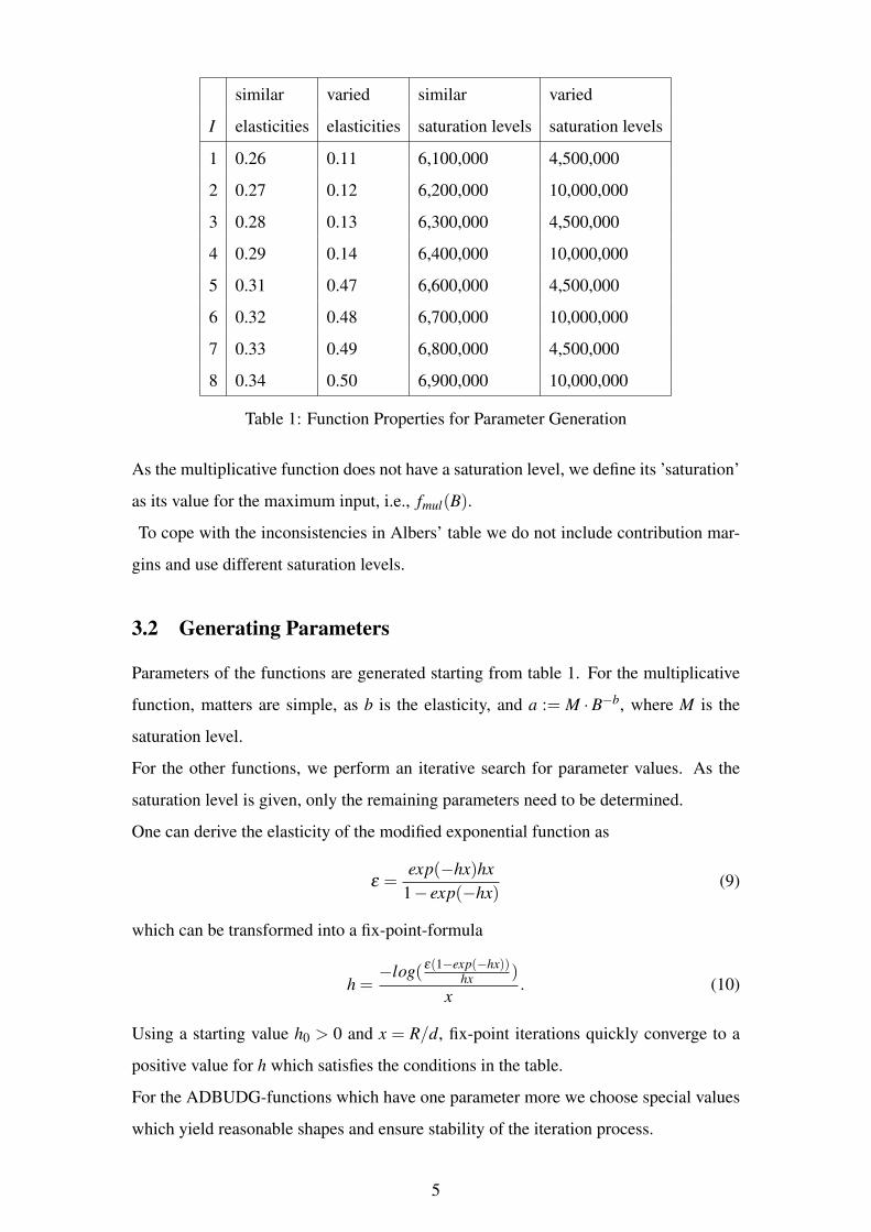
similar varied similar varied

I elasticities elasticities saturation levels saturation levels

1 0.26 0.11 6,100,000 4,500,000

2 0.27 0.12 6,200,000 10,000,000

3 0.28 0.13 6,300,000 4,500,000

4 0.29 0.14 6,400,000 10,000,000

5 0.31 0.47 6,600,000 4,500,000

6 0.32 0.48 6,700,000 10,000,000

7 0.33 0.49 6,800,000 4,500,000

8 0.34 0.50 6,900,000 10,000,000

Table 1: Function Properties for Parameter Generation

As the multiplicative function does not have a saturation level, we define its ’saturation’

as its value for the maximum input, i.e., fmul(B).

To cope with the inconsistencies in Albers’ table we do not include contribution mar-

gins and use different saturation levels.

3.2 Generating Parameters

Parameters of the functions are generated starting from table 1. For the multiplicative

function, matters are simple, as b is the elasticity, and a := M ·B−b, where M is the

saturation level.

For the other functions, we perform an iterative search for parameter values. As the

saturation level is given, only the remaining parameters need to be determined.

One can derive the elasticity of the modified exponential function as

ε =exp(−hx)hx

1− exp(−hx)(9)

which can be transformed into a fix-point-formula

h =−log( ε(1−exp(−hx))

hx)

x. (10)

Using a starting value h0 > 0 and x = R/d, fix-point iterations quickly converge to a

positive value for h which satisfies the conditions in the table.

For the ADBUDG-functions which have one parameter more we choose special values

which yield reasonable shapes and ensure stability of the iteration process.

5

3.3 Disturbances

To each function we add normally distributed disturbances u∼N (0,σ2). Variances σ2

are set to attain a desired share of explained variance for the dependent variable sales.

These desired R2 values amount to 0.9,0.7, and 0.5. For each function the error variance

σ2 is set to the value which leads the R2-value closest to its desired value in a regression

of that function using 2,000 uniformly distributed integer values of the inputs.

3.4 Rules of Thumb

We start from the same rules of thumb as Albers (1998):

1. Allocation proportional to sales of a unit in the previous period.

2. Allocation proportional to sales of a unit divided by its allocation in the previous

period.

3. Allocation proportional to the saturation level of a unit.

The third rule cannot be implemented as saturation levels like all parameters of func-

tions are unknown. That is why we replace it by the following rule.

3.’ Allocation proportional to maximum sales of a unit observed so far.

For the remainder of the paper we will refer to these as first, second and third rule of

thumb.

3.5 Estimators for Elasticities

On the basis of several definitions of point and arc elasticity to be found in the literature

(see, e.g., Vazquez (1995) P.223 and Seldon (1986) P.122) we obtain four different

estimators:

log( y2

y1)

log( x2x1),

y2−y1

y1

x2−x1x1

,

y2−y1

y2

x2−x1x2

,

y2−y1

y

x2−x1x

(11)

where x := x1+x22

and y := y1+y2

2.

x1 and x2 denote inputs of two consecutive periods, y1 and y2 their corresponding out-

puts (sales).

6

The results we present later are obtained using the third estimator which leads to highest

values for the objective “Sales” (see section 5). But note that the difference to the other

three estimators is not statistically significant according to a regression analysis with

main effects only.

3.6 Elimination of correlation conditions

Albers also compares different starting conditions with respect to the correlation of

starting allocations with their optimal values. These starting conditions are constructed

by changing an equal distribution by roughly 5% towards a positive or negative corre-

lation to the optimum. However, this only makes sense in a situation without random

disturbances. In our case, the magnitude of the error terms, even in the case of R2 = 0.9,

greatly exceed a 5% boundary and hence these starting condition variations need not be

considered. Therefore the starting allocations are equal with B/8 = 1,000,000 for each

unit.

4 Developed Algorithm

Albers (1998) intends to show that in allocation problems iterations along elasticities

always outperform rules of thumb, independent from functional form, other properties

of the functions and correlations of starting values with optimal allocations. He consid-

ers for each of the four functions discussed in the previous section every constellation

of different values of properties and correlations. Sales are computed on the basis of

these functions without adding disturbances though the latter are a component of most

econometric models, Results obtained by his iterative algorithm are compared to those

computed by the three rules of thumb explained in the previous section. Overall, his

iterative algorithm outperforms all rules of thumb by far.

In our study the algorithm of Albers turns out not to work well for sales response func-

tions with additive disturbances. Disturbances which directly affect elasticities cause

elasticities and new allocation values to fluctuate. Very small allocations are computed

quite often which in their turn lead to a low function value before a disturbance is added.

Under such circumstances adding a disturbance frequently results in a negative value

and the logarithmic estimator of elasticities which is used in the algorithm of Albers

does not work. But note that any of the other three estimators shown in section 3.5 also

leads to heavily biased, sometimes even negative, elasticities.

7

4.1 Exploration

In order to bring stability to the process, we apply first order exponential smoothing in

the following way:

εt := (1−β )εt−1 +β εt (12)

with β ∈ [0,1] (we use β := 0.85 based on a comparison of different values).

εt is the smoothed elasticity and εt the estimated elasticity in period t. Moreover, each

elasticity value is projected into the interval [0.01,0.5], i.e., if the calculated value is

above 0.5 it was set to 0.5, and it was set to 0.01 if it was below 0.01.

So far we have described the exploration phase of the algorithm. As allocations gener-

ated in this fashion are close to the optimum we consider it to be useful for exploration.

But even the exponential smoothing version still jumps around too much. Therefore

there is dire need for a method which dampens disturbances.

4.2 Exploitation

The general idea can be easily understood when looking at modified exponential func-

tions with varying parameters. The optimal allocation for the function in the example

drawn in figure 1 is roughly 640,000. Nevertheless, even when the error term is small,

the algorithm and each of the three rules of thumb still fluctuate a lot, showing no sign

of stability, although they do not leave a certain interval of the domain in each variable

(and hence of the codomain).

This area shown in the figure looks like it can be easily approximated by a parabola,

i.e. a polynomial of degree two. Assuming the functions were actually polynomials of

degree two, quadratic programming could then give an exact solution, as the boundary

condition is linear.

The two steps necessary for optimization are hence: exploration and exploitation, a con-

cept first introduced by March (1991) . During a fixed number of periods, the algorithm

generates data points close enough to the optimum. After that, a quadratic regression of

the form

y ∼ ax2 +bx+ c (13)

is performed for each unit in order to approximate its unknown function based on all

values of sales and allocations available so far (using a smaller number of the most

8

●

●

●

●

●

●

●

●

●

●

●

●

●

●

●

●

●

●

●

●

●

●

●

●

●

●

●

●

●

●●

●●

●●

●●

●●

●●

●●

●●

●●

●●

●●

●●●●●●●●●●●●●●●●●●●●●●●●●●●●●●●●●●●●●●●●●●●●●●●●●●

x/10000

y/1

00

00

0 50 100 150 200 250 300

05

01

00

15

02

00

25

03

00

35

04

00

45

0

● true function

fitted parabola

Figure 1: True Function and Fitted Parabola

recent values only does not improve results). Then quadratic programming yields an

allocation which is optimal for these approximations, obeys the total resource restric-

tion and provides a new data point for the regression. We use the method of Goldfarb

and Idnani (1983) for quadratic programming in our implementation. This process is

repeated until a total of 40 iterations is reached.

A problem arises when a is estimated as a positive number for any sales unit, as the

matrix in the quadratic program is no longer positive definite. This, however, has a

surprisingly easy fix: a can be set to a very small value (we choose −10−15) and b is

set to the slope of a linear regression line, thereby “fooling” the quadratic program into

accepting something that is basically a straight line rather than a parabola.

In the worst-case-scenario, additionally, the slope of the regression line may be nega-

tive. This case is very rare and the allocation to this unit will almost certainly be zero.

One should remember however, what this actually means: The shape of the data points

resembles a monotonically decreasing, convex (!) function and would hence arise either

from a few very unlucky error terms in a row or an outer influence that cannot be ex-

9

plained by an additive error term. Surely in this case the function should be thoroughly

analyzed instead of continuing the application of any algorithm.The situation will be

briefly mentioned in section 6.

A final question that arises is when to switch from exploration to exploitation. As the

exact functions and variances are unknown to the algorithm, there can be no mathemat-

ical derivation of the optimal switching point. The main idea is that for higher error

variances, more exploration is necessary to make sure the parabolas are sufficiently ac-

curate. This was confirmed in a separate simulation wherein the R2-Levels of 0.9,0.7

and 0.5 optimally had 10, 14 and 18 iterations respectively. Hence, an estimator for

the switching period was defined based on these results, dependent on the estimated

variance of the data. After the first nine iterations, this number is estimated, and lies in

the interval [10,25].

4.3 Related Allocation Problem

The form of the investigated allocation problem presented in section 2 also gives rise to

the solution of a different, but related problem for free. In the related decision problem

one part of a given budget B may be spent (allocated), while the other part may be saved.

Instead of (2) we obtain the following objective function

n∑

i=1

fi(xi)+(B−

n∑

i=1

xi). (14)

in which the remaining, unspent budget B−∑n

i=1 xi is added to the sum of sales across

all units.

This problem looks different from the one we have investigated so far, but rewritten it

turns out to be just a special case. Define the function fn+1(x) := x, and consider the

allocation of B onto the n+1 functions f1, ..., fn+1. A complete allocation now means

finding (x′1, ...,x′n+1) that sum up to B. But that is equivalent to finding (x1, ...,xn) that

sum up to a value R ≤ B, since we can then put x′1 := x1, ...,x′n := xn,x

′n+1 := B−R, and

they evidently add up to B.

So now we can see that this problem can be solved by the algorithm discussed above,

but we know even more: as fn+1(x) = x, its elasticity is exactly 1 and hence need not

be estimated, no problems arise in the exploration phase. As fn+1 is a straight line, we

use the fix discussed in 4.2 by adding a tiny parabola to make it compatible with the

quadratic program. As this function has no additive disturbance, the problem is actually

easier to solve than a regular allocation to n+1 units. The optimum is found when the

10

slopes of all functions are equal to one (as the Lagrange-multiplier becomes 1, see A.3)

and the remaining budget is saved. This is to be expected, as the slope of f (x) = x is

constant 1 and every further unit of the budget will be added to the function with the

steepest slope.

5 Evaluation of Procedures

We want to compare four different procedures, i.e., three rules of thumb and the algo-

rithm introduced in section 4. To this end we conduct a simulation study and consider

two different dependent variables which both are computed as arithmetic means across

40 periods. The first dependent variable “Sales” is based on total sales attained by rules

of thumb or the algorithm in each period. The second dependent variable “Optimality”

is a relative measure, the ratio of total sales and optimal total sales. Optimal total sales

are determined by optimizing on the basis of the true response functions without dis-

turbances, i.e., assuming knowledge of sales response functions and their parameters.

Optimality therefore shows to what extent a procedure which lacks knowledge of the

response functions attains optimal total sales on average. A value of 1.0 for optimality

indicates as a rule that average total sales equal their optimal value.

As mentioned above, the S-shaped ADBUDG-function is not concave, and hence a

problem arises with local and global optima. In particular, the nine control algorithms

that search for the optimal solution may get stuck in local optima. Therefore optimali-

ties greater than 1.0 maybe obtained.

We look at 192 constellations, which result from four function types, four procedures,

similar/varied elasticities, similar/varied saturations, three error levels and generate five

replications for each constellation. A seed is set to ensure reproducibility.

The dependent variables are normalized in the following manner: As “Optimality” usu-

ally is already a number between 0 and 1, no normalization is necessary. Since the

four function types yield quite different values for total sales (which is especially pro-

nounced for the ADBUDG-functions), “Sales” are divided by the maximum value of

the respective function type. This allows to compare the effectiveness of procedures

across different functional forms.

Finally, two linear regressions are performed in the following way:

11

Sales ∼ β1,0 +β1,1Proc+β1,2Form+β1,3Dist +β1,4Elas+β1,5Satu (15)

Optimality ∼ β2,0 +β2,1Proc+β2,2Form+β2,3Dist +β2,4Elas+β2,5Satu (16)

All independent variables are categorical, where “Proc” takes values corresponding to

the three rules of thumb and the algorithm described above, “Form” takes the four values

corresponding to the four types of functions, “Dist” takes three values corresponding to

the R2 values of 0.9,0.7 and 0.5, and “Elas” and “Satu” take two values corresponding

to “similar” and “varied”, as explained above.

Moreover, we also estimate regression models which in addition include certain sets

of interaction terms. As models with main effects only are inferior to models with

interactions, a discussion of the main effect regressions can be found in Appendix C.

5.1 Results for Regression Models with Interactions

We consider several model types with interaction terms. The most simple of these

models includes only pairwise interactions of the “Procedure”-variable with all other

variables. In this model we can easily analyze the interactions between procedures and

the other variables, while also, with the use of F-tests, being able to compare the perfor-

mance of procedures (results of these models and models with all pairwise interactions

can found in Appendix C).

To consider additional interaction terms we also investigate models(one for each depen-

dent variable) with all pairwise interactions and models with double, triple, quadruple

and quintuple interactions. Quite interestingly, the full models with quintuple inter-

actions not only lead to the best variance explanations (adjusted R2 values amount to

0.8786 and 0.85 for “Sales” and “Optimality”, respectively), but F-tests also confirm

that the full models outperform all the restricted models.

A complete explanation of the F-tests used to compare procedures is given in Appendix

C section C.3, here we present the main results.

These comparisons consist of two steps ( C.2 is a more comprehensive example, since

it has fewer coefficients and a simpler null hypothesis). In the first step we calculate

the effect of each procedure by summing all its interaction terms. Then for each pair of

procedures we subtract their two respective effects (for a detailed explanation see the

example in section C.2). The corresponding matrix (whose product with the coefficient

vector is zero under the null hypothesis) was the basis of an F-test. Hence the sign of

12

the difference indicates if the algorithm performs better than a rule of thumb, and the

F-statistic reveals the significance of a difference .

For the dependent variable “Sales” we obtain average differences between the algo-

rithm and each of the three rules of thumb of 4.8325, 7.2464, and 3.7383, respectively.

These differences are highly significant at levels lower than 0.001 (the corresponding

F-statistics are 46.426, 104.389 and 27.782). Based on these results we conclude that

the algorithm clearly beats the three rules of thumb in terms of Sales.

For the other dependent variable “Optimality” we obtain differences of -0.9251, 1.7389

and -2.2644 (F-statistics are 1.4663, 5.1813 and 8.7861), respectively. At a significance

level of 0.05 the algorithm performs better than the second rule of thumb, but worse

than the third rule of thumb. In addition no significant performance difference with

respect to the first rule of thumb is found.

5.2 Discussion

We begin by discussing the results for “Sales”. As seen in the full model, the algorithm

is vastly superior to all three rules of thumb. This is the most important result, which

leads to clear implications for marketing decisions: Whenever a scarce resource needs

to be allocated to different units, it is highly beneficial to use all the data like in the

algorithm, instead of considering only the most recent observation like in the rules of

thumb investigated here. In applying our algorithm two situations can be distinguished.

If historical data with enough variation are lacking, begin with exploration and switch

to exploitation later on. If on the other hand appropriate historical data are at hand,

one may start with the exploitation stage right away, i.e., use quadratic regression and

quadratic optimization. This approach should highly improve “Sales” as compared to

its value obtained by rule of thumbs.

With respect to “Optimality” we obtain much lower F-statistics for procedure compar-

isons, probably due to the fact that this dependent variable is limited to the unit interval

with respect to a global maximum. As long as procedures do not behave chaotically,

not a lot of variance and difference between algorithms can be expected. This will be

discussed shortly, but first let us consider the results.

As no significant difference can be seen between the algorithm and the first rule of

thumb, no further discussion is necessary here. The second rule is outperformed be-

cause of certain chaotic patterns that can be visualized by manually starting optimiza-

13

tions with low levels of R2. We can see that our algorithm clearly outperforms the

second rule of thumb both with respect to “Sales” and “Optimality”. This disadvantage

of the second rule of thumb is also confirmed by the second and hence by both F-tests

explained above. The third rule of thumb leaves us with mixed signals. While we seem

to obtain significantly better sales with our algorithm, the third rule seems to perform

significantly closer to the optimum. This is not as contradictory as it first seems, since

the rule literally says: “take the highest value you can get” but might then refuse to

move from the position it has settled in.

We see three reasons for not using the third rule of thumb:

1. The rule should not be used if decision makers have more interest in high achieved

sales and do not care how close sales are to an optimal value which is based on unknown

functions and ignores disturbances. This recommendation follows from the results of

our simulation study for the objective “Sales” which clearly show that the algorithm

performs better.

2. The rule cannot be modified to deal with extended marketing decision problems (e.g.,

if an allocation affects other units as well, if sales depend on marketing variables of dif-

ferent types, etc.) which may be investigated by future research. We shortly discuss

several extensions in the next section and indicate that the algorithm can be modified to

handle these more general problems.

3. This rule uses almost no information from previous periods to determine the alloca-

tion.

In Albers’ original version it was just defined as the allocation proportional to the satu-

ration levels, which as a rule are not known in practice. Providing examples of functions

for which this rule of thumb behaves very badly is rather simple. For example, given a

resource of 700,000 and eight S-shaped ADBUDG-functions with different elasticities

and varied saturation levels and medium disturbances the third rule leads to solutions

which are clearly worse compared to those determined by our algorithm (see table 2).

This weakness of the third rule can be consistently observed if ressources are low.

6 Conclusions

In addition to the simulation study presented we examine whether performance of the

developed algorithm remains stable if it has to deal with different conditions. First of all

we analyze how procedures behave given a different number of units. The performance

14

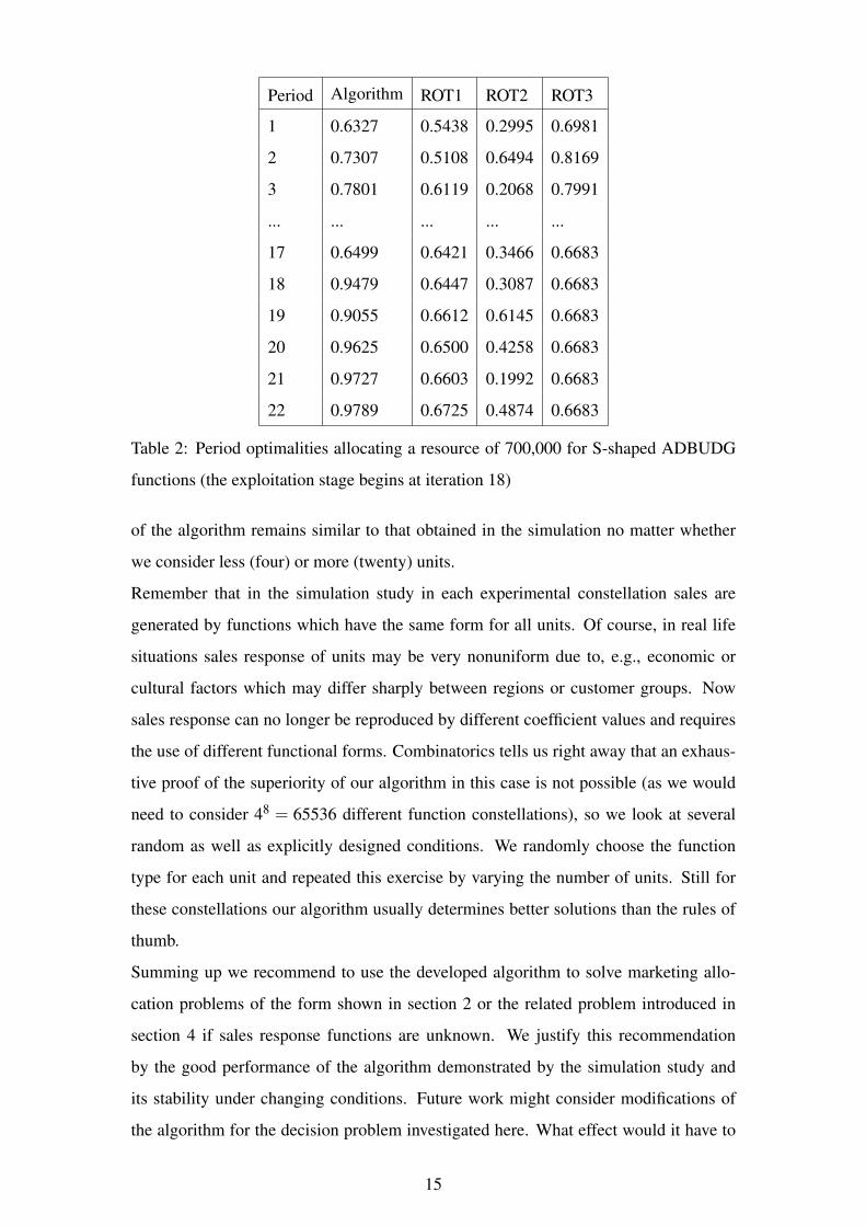
Period Algorithm ROT1 ROT2 ROT3

1 0.6327 0.5438 0.2995 0.6981

2 0.7307 0.5108 0.6494 0.8169

3 0.7801 0.6119 0.2068 0.7991

... ... ... ... ...

17 0.6499 0.6421 0.3466 0.6683

18 0.9479 0.6447 0.3087 0.6683

19 0.9055 0.6612 0.6145 0.6683

20 0.9625 0.6500 0.4258 0.6683

21 0.9727 0.6603 0.1992 0.6683

22 0.9789 0.6725 0.4874 0.6683

Table 2: Period optimalities allocating a resource of 700,000 for S-shaped ADBUDG

functions (the exploitation stage begins at iteration 18)

of the algorithm remains similar to that obtained in the simulation no matter whether

we consider less (four) or more (twenty) units.

Remember that in the simulation study in each experimental constellation sales are

generated by functions which have the same form for all units. Of course, in real life

situations sales response of units may be very nonuniform due to, e.g., economic or

cultural factors which may differ sharply between regions or customer groups. Now

sales response can no longer be reproduced by different coefficient values and requires

the use of different functional forms. Combinatorics tells us right away that an exhaus-

tive proof of the superiority of our algorithm in this case is not possible (as we would

need to consider 48 = 65536 different function constellations), so we look at several

random as well as explicitly designed conditions. We randomly choose the function

type for each unit and repeated this exercise by varying the number of units. Still for

these constellations our algorithm usually determines better solutions than the rules of

thumb.

Summing up we recommend to use the developed algorithm to solve marketing allo-

cation problems of the form shown in section 2 or the related problem introduced in

section 4 if sales response functions are unknown. We justify this recommendation

by the good performance of the algorithm demonstrated by the simulation study and

its stability under changing conditions. Future work might consider modifications of

the algorithm for the decision problem investigated here. What effect would it have to

15

choose a different algorithm in the exploration phase? A next goal would be to check

if other algorithms are more suitable for the exploitation phase. This might mean small

adjustments of parameters, or a completely new algorithm.

As mentioned in section 4, a problem arises if the parabola has a positive leading co-

efficient and the regression line has a negative slope. This effect usually occurs if a

unit repeatedly receives allocations near zero. Due to the additive disturbances the data

set for the regressions then consists of very similar x-values, while the y-values vary a

lot. As low allocations are usually not optimal, an amendment of the algorithm may be

benefical for such situations.

Modifying the algorithm to solve more general marketing decision problems also seems

to be an interesting task of future research. One extended decision problem results if

one or several sales functions may change suddenly. We suspect that under such circum-

stances the exploration phase will have to start once again. For situations with gradual

change on the other hand an easy fix would be to delete older data points before each it-

eration. One could also investigate multi-variable generalizations. In one generalization

allocations affect sales of the same unit as well as sales of other units. Another more

challenging generalization allows for marketing variables of different types. Examples

of such variables are advertising and price or advertising and sales effort, where both

variables have an effect on sales of different units.

A Appendix: Mathematical Discussion

This section is a repetition of the results from Albers (1998).

As mentioned above, a scarce resource B is to be allocated to n different units, where

we want to find the maximum objective

max

n∑

i=1

fi(xi) (A.1)

of all allocations (x1, ...,xn).

The most suitable mathematical context for this problem is the Lagrangian formalism

for optimizing a function (2) with a given condition (3).

16

A.1 Albers’ Lagrange-Ansatz

The Lagrangian one needs to consider takes the form

L =

n∑

i=1

fi(xi)+λ · (

n∑

i=1

xi −B), (A.2)

and one shall differentiate (A.2) by the xi and λ and set the derivations equal to zero to

get the conditions an extremum needs to satisfy.

One receives

∂L

∂xi=

∂ fi

∂xi−λ

!= 0 (A.3)

and of course∑

i∈I

xi = B. (A.4)

As the point elasticity is defined as∂ fi∂xi

· xi

fi= εi we can rewrite

∂ fi∂xi

as εi ·fixi

and insert

into (A.3)

εi ·fi

xi= λ ⇒ xi =

fiεi

λ. (A.5)

In particular, the resource becomes

B =∑

i∈I

xi =∑

i∈I

fiεi

λ, (A.6)

which can be solved for λ and inserted into (A.5) to obtain

xi =fiεi∑

j∈I f jε jB. (A.7)

In general, the exact form of the functions fi, in particular its point elasticity is unknown.

However, given two values xi and x′i, and their respective outputs yi = fi(xi),y′i = fi(x

′i)

, the arc elasticity may be estimated as

εi =ln( yi

y′i)

ln( xi

x′i), (A.8)

where ln is the natural logarithm. Of course, other estimators may be used here as well,

as explained above. This gives rise to an iterative algorithm, where in each step the

elasticities are estimated dependent on the last two iterations and the components xi of

the new allocation (x1, ...,xn) are obtained from that elasticity.

17

A.2 Further results

As the functions are concave and the process closes in on the Lagrange solution, the

method presented will find a solution to the allocation problem, if it exsists. To guar-

antee the existence of a (unique) solution, a descent into mathematics is necessary. If

the reader is unfamiliar with concepts of continuity, compactness and the extreme value

theorem for topological spaces (or subsets of Rn) he may consult Rudin (1976).

Neither negative inputs nor outputs are to be expected, so consider R+0 := {x∈R|x≥ 0}.

Definition 1

A function f : R+0 → R

+0 satisfies the conditions of diminishing returns, if

1. f ∈C2(R+0 ) (double differentiability)

2. f ′(x)≥ 0 ∀x∈R+0

(monotony)

3. f ′′(x)< 0 ∀x∈R+0

(strict concavity)

(This condition may actually be weakened. We only require single differentiability;

condition 3 then becomes “ f ′ is strictly monotonically decreasing”)

A.3 Existence

Proposition 1

Let ( fi)i∈I be a finite family (#I = n) of continuous functions. Then for every B > 0 there

is a solution to the allocation problem (2) & (3).

Proof:

The map

F : (R+0 )

n → R+0 ,(xi)i∈I 7→

n∑

i=1

fi(xi) (A.9)

is continuous, since the fi are, which follows from Rudin P.87 Theorem 9 and Theorem

10 . The bounded hyperplane

H := {(xi)i∈I|

n∑

i=1

xi = B} (A.10)

is a closed (in the topological sense; this is equivalent to “the limit of every convergent

sequence with terms in H also lies in H”; the reader may varify that H is in fact closed,

by using that the function (x1, ...,xn) 7→∑n

i=1 xi is sequentially continuous) subset of

(R+0 )

n and hence compact (by the Heine-Borel-theorem, see Rudin P.40 Theorem 2.41).

The restriction of F to H is continuous as well, since continuity is a local property.

18

Since every continuous function from a compact set to R attains its maximum (see

Rudin P.89/90 Theorem 4.16), so does F|H which ends the proof. ✷

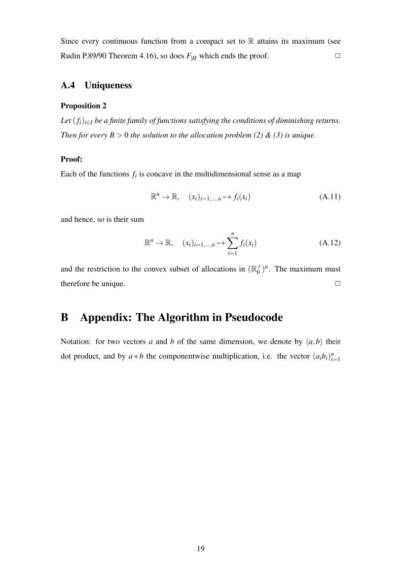
A.4 Uniqueness

Proposition 2

Let ( fi)i∈I be a finite family of functions satisfying the conditions of diminishing returns.

Then for every B > 0 the solution to the allocation problem (2) & (3) is unique.

Proof:

Each of the functions fi is concave in the multidimensional sense as a map

Rn → R, (xi)i=1,...,n 7→ fi(xi) (A.11)

and hence, so is their sum

Rn → R, (xi)i=1,...,n 7→

n∑

i=1

fi(xi) (A.12)

and the restriction to the convex subset of allocations in (R+0 )

n. The maximum must

therefore be unique. ✷

B Appendix: The Algorithm in Pseudocode

Notation: for two vectors a and b of the same dimension, we denote by 〈a,b〉 their

dot product, and by a ∗ b the componentwise multiplication, i.e. the vector (aibi)ni=1

19

Data: x1 = (x11, ...,x

1n), x2 start values, 0 ≤ β ≤ 1 smoothing parameter, maxit:

maximum number of iterations, B: resource, In: identity matrix of

dimension n, exex=10: first estimate of number of iterations in exploration

phase, f : multidimensional map consisting of the separate functions in

each component, DF : array which will be filled with the data points of all

functions

y1 := f (x1);y2 := f (x2);

while i < exex do

Test(x1,x2,y1,y2);

ε :=y2−y1

y1

x2−x1

x1

; Epstest(ε) ;

if i ≥ 2 then

εsm := ε · (1−β )+ εold ·β

else

εsm := ε;

end

up := y1∗εsm

〈y1,εsm〉·B;

εold := εsm;

x2 := x1;y2 := y1;

Test2(up,x2);

x1 := up;y1 := f (x1);

if i = 9 then

estimate variance and exex

end

add (x1,y1) to DF ;

end

for i = exex to maxit do

for j = 1 to n do

Perform Regression y j ∼ a(x j)2 +bx j + c

end

D: Diagonal Matrix containing a-values·(−2)

A: n by n+1-Matrix with −1 in the first column followed by In

d: Vector containing b-values

bv: Vector of length n+1 containing (−B,0,0, ...,0)

up:=solve.QP(D,d,A,bv)

x1 := up;y1 := f (x1);

add (x1,y1) to DF ;

end

20

Remark: The functions Test and Test2 check if the entries are too small or too close to

each other, epstest projects elasticities into the Interval [0.01,0.5].

Note that the estimator for “exex” was determined empirically and is directly dependent

on maxit

The function solve.QP solves the quadratic program as described in Goldfarb/Idnani

(1983) with the notation from the R-Package “quadprog”.

21

Dependent Variable: Sales Dependent Variable: Optimality

Variable Coefficient t-Value Coefficient t-Value

Intercept 0.881 118.582*** 1.023 128.317***

Proc2 -0.014 -2.271* -0.017 -2.510*

Proc3 -0.065 -10.209*** -0.073 -10.676***

Proc4 0.008 1.328 0.011 1.595

Form2 0.034 5.306*** 0.024 3.462***

Form3 0.102 16.171*** 0.034 5.030***

Form4 -0.009 -1.401 -0.020 -2.896**

Dist2 -0.018 -3.324*** -0.021 -3.636***

Dist3 -0.047 -8.573*** -0.057 -9.722***

Elas2 -0.021 -4.762*** -0.051 -10.544***

Satu2 0.058 12.882*** -0.040 -8.332***

* p-value<0.05, ** p-value<0.01, *** p -value<0.001

Table 3: Main Effect Regression Models

C Appendix: Detailed Regression Results

C.1 Main effect models

The regression results of the main effect models both for “Sales” and “Optimality”

are shown in table 3. The independent variables are coded by binary dummy variables

with the developed algorithm, the multiplicative function, similar elasticities and similar

saturations as reference categories.

C.2 Models with procedure interactions

In addition to main effects we now consider pairwise interaction between procedures

and each of the other independent variables. We compute the total effect of our algo-

rithm in the following manner. We add the intercept to each main effect coefficient and

sum these intermediate values. To this sum we add the intercept once more to also con-

sider the constellation in which all independent variables are in their reference category.

The first rule of thumb would be represented by the coefficients of the interactions of

the rule of thumb with each condition plus the coefficient of the rule of thumb plus

intercept, plus another sum of the rule of thumb plus intercept. For the corresponding

22

F-test we construct a matrix that, when multiplied with the coefficient vector, gives us

the difference of these two real numbers, where the null hypothesis is that number be-

ing zero. The matrix is hence a 1x32 matrix with a -8 in second entry, a 1 in entries

(5,6,7,8,9,10,11), a -1 in entries (12,15,18,21,24,27,30), and zeroes elsewhere.

The resulting coefficient for “Sales” is 0.2073 , implying that the algorithm is better than

the first rule of thumb. The F-statistic takes the value 9.4066 and follows an F(1,928)-

distribution given the null hypothesis. Therefore the algorithm is better than the first

rule of thumb at a significance level of 0.0022. Furthermore it outperforms the third

rule of thumb with respect to “Sales” with a p-value of 0.056 and the second rule of

thumb with respect to optimalities with a p-value of 0.025.

C.3 F-Tests in the Full Models

In order to compare the strengths of the algorithms in the full model, F-Tests were

performed in the following manner. The coefficient vector of the OLS-Estimator was

multiplied with a matrix representing the difference of the algorithms. This matrix was

constructed analogously to the ones in the previous section: For every constellation of

conditions a matrix was defined as the sum of the coefficients containing the algorithm

together with the corresponding interaction terms minus the coefficients containing the

rule of thumb that was to be discussed, again, including their respective interactions.

All these matrices were added yielding three matrices, one for each rule of thumb. This

data is represented in table 4, where the variables are shortened to their first letter.

The coefficients in the table hence represent the number of effects it appears in (as the

null hypothesis is the difference of sums of the effects). Hence if ki is the number

of categories of the variable i, the number of the effects the l-fold interaction term

i1 × ...× il appears in (for l ∈ {0, ...,5}), is

∏

i/∈{i1,...,il}

ki. (C.1)

For example, the interaction term P1 : F2 : D2 : E1 appears in its own effect (together

with lower terms) where S= 2 (as S2 is the reference category) and its counterpart where

S = 1, represented by itself, lower terms and the coefficient of P1 : F2 : D2 : E2 : S2.

Via the formula we get

∏

i/∈{F,D,E}

ki =∏

i∈{S}

ki = kS = 2. (C.2)

23

Name β1 β2 M1 M2 M3 Name β1 β2 M1 M2 M3

(Intercept) 0.82277 0.99693 0 0 0 P3:F4:S1 0.01025 0.00945 0 0 -6

P1 -0.00588 -0.00007 -48 0 0 P1:D2:S1 -0.02060 -0.00951 -8 0 0

P2 0.00250 -0.00070 0 -48 0 P2:D2:S1 -0.13402 -0.13451 0 -8 0

P3 -0.00285 0.00094 0 0 -48 P3:D2:S1 -0.00755 -0.00361 0 0 -8

F2 0.05685 -0.00393 12 12 12 P1:D3:S1 0.02295 -0.00087 -8 0 0

F3 0.13735 -0.00244 12 12 12 P2:D3:S1 -0.22894 -0.26788 0 -8 0

F4 0.04394 -0.00504 12 12 12 P3:D3:S1 0.00415 0.00721 0 0 -8

D2 -0.01137 -0.00690 16 16 16 F2:D2:S1 -0.02247 -0.01135 2 2 2

D3 0.00722 -0.01061 16 16 16 F3:D2:S1 -0.00932 -0.00337 2 2 2

E1 0.00765 -0.05026 24 24 24 F4:D2:S1 -0.02821 -0.03078 2 2 2

S1 0.11797 -0.00405 24 24 24 F2:D3:S1 0.00805 -0.00366 2 2 2

P1:F2 0.01079 0.00578 -12 0 0 F3:D3:S1 0.01135 0.01056 2 2 2

P2:F2 0.00172 0.00520 0 -12 0 F4:D3:S1 0.01334 0.00228 2 2 2

P3:F2 0.00915 0.00554 0 0 -12 P1:E1:S1 -0.00701 0.00069 -12 0 0

P1:F3 0.00670 0.00368 -12 0 0 P2:E1:S1 -0.01137 -0.01288 0 -12 0

P2:F3 -0.00379 0.00352 0 -12 0 P3:E1:S1 -0.00836 -0.00124 0 0 -12

P3:F3 0.00290 0.00280 0 0 -12 F2:E1:S1 -0.00561 0.00644 3 3 3

P1:F4 0.00852 0.00575 -12 0 0 F3:E1:S1 -0.02180 -0.00900 3 3 3

P2:F4 -0.00041 0.00452 0 -12 0 F4:E1:S1 0.03958 0.02374 3 3 3

P3:F4 0.00769 0.00642 0 0 -12 D2:E1:S1 0.00931 0.00566 4 4 4

P1:D2 0.01757 0.00264 -16 0 0 D3:E1:S1 0.05078 0.04154 4 4 4

P2:D2 0.00401 -0.00052 0 -16 0 P1:F2:D2:E1 0.03734 0.01509 -2 0 0

P3:D2 0.00485 0.00678 0 0 -16 P2:F2:D2:E1 0.01296 0.02702 0 -2 0

P1:D3 -0.02295 -0.01215 -16 0 0 P3:F2:D2:E1 -0.00739 -0.00683 0 0 -2

P2:D3 -0.06001 -0.07274 0 -16 0 P1:F3:D2:E1 0.02650 0.01755 -2 0 0

P3:D3 -0.00095 0.00907 0 0 -16 P2:F3:D2:E1 0.00549 0.03205 0 -2 0

F2:D2 0.00771 0.00420 4 4 4 P3:F3:D2:E1 -0.00878 -0.00335 0 0 -2

F3:D2 0.00903 0.00705 4 4 4 P1:F4:D2:E1 0.01622 0.00747 -2 0 0

F4:D2 -0.00071 0.00061 4 4 4 P2:F4:D2:E1 0.00529 0.02670 0 -2 0

F2:D3 -0.02408 -0.00006 4 4 4 P3:F4:D2:E1 -0.01882 -0.00812 0 0 -2

F3:D3 -0.01386 0.00868 4 4 4 P1:F2:D3:E1 -0.04176 -0.02704 -2 0 0

F4:D3 -0.04265 -0.02514 4 4 4 P2:F2:D3:E1 0.07127 0.11882 0 -2 0

P1:E1 -0.01688 -0.02401 -24 0 0 P3:F2:D3:E1 -0.04038 -0.02815 0 0 -2

P2:E1 0.00566 0.01336 0 -24 0 P1:F3:D3:E1 -0.03123 -0.01473 -2 0 0

P3:E1 0.00566 -0.00240 0 0 -24 P2:F3:D3:E1 0.06680 0.10899 0 -2 0

F2:E1 -0.03689 0.03150 6 6 6 P3:F3:D3:E1 -0.02832 -0.03552 0 0 -2

F3:E1 0.02150 0.01499 6 6 6 P1:F4:D3:E1 -0.04615 -0.03372 -2 0 0

F4:E1 -0.06042 0.01980 6 6 6 P2:F4:D3:E1 -0.03058 -0.02472 0 -2 0

D2:E1 -0.00439 -0.01031 8 8 8 P3:F4:D3:E1 -0.02570 -0.04034 0 0 -2

D3:E1 -0.04049 -0.03881 8 8 8 P1:F2:D2:S1 0.02769 0.00794 -2 0 0

P1:S1 0.01147 0.00334 -24 0 0 P2:F2:D2:S1 0.14667 0.14205 0 -2 0

P2:S1 -0.00663 -0.00812 0 -24 0 P3:F2:D2:S1 0.02404 0.02016 0 0 -2

P3:S1 0.00542 0.00170 0 0 -24 P1:F3:D2:S1 0.02292 0.01260 -2 0 0

F2:S1 -0.02037 -0.00832 6 6 6 P2:F3:D2:S1 0.12912 0.13675 0 -2 0

F3:S1 -0.11627 0.00533 6 6 6 P3:F3:D2:S1 0.00472 0.00639 0 0 -2

F4:S1 -0.02085 -0.02512 6 6 6 P1:F4:D2:S1 0.05832 0.05041 -2 0 0

D2:S1 0.00910 0.00030 8 8 8 P2:F4:D2:S1 -0.00869 -0.00287 0 -2 0

D3:S1 -0.01624 -0.01329 8 8 8 P3:F4:D2:S1 0.02224 0.03694 0 0 -2

E1:S1 0.00649 -0.00382 12 12 12 P1:F2:D3:S1 -0.01288 -0.00345 -2 0 0

P1:F2:D2 -0.01831 -0.00332 -4 0 0 P2:F2:D3:S1 -0.01396 0.01430 0 -2 0

P2:F2:D2 -0.00501 -0.00189 0 -4 0 P3:F2:D3:S1 0.01623 0.02089 0 0 -2

P3:F2:D2 -0.00391 -0.00503 0 0 -4 P1:F3:D3:S1 -0.02459 0.00289 -2 0 0

P1:F3:D2 -0.01561 -0.00405 -4 0 0 P2:F3:D3:S1 0.21926 0.26922 0 -2 0

P2:F3:D2 -0.00069 -0.00164 0 -4 0 P3:F3:D3:S1 -0.00413 -0.00461 0 0 -2

P3:F3:D2 -0.00034 -0.00705 0 0 -4 P1:F4:D3:S1 0.02709 0.05167 -2 0 0

P1:F4:D2 -0.01683 -0.00600 -4 0 0 P2:F4:D3:S1 -0.18091 -0.17894 0 -2 0

P2:F4:D2 -0.00673 -0.00852 0 -4 0 P3:F4:D3:S1 0.00778 0.01419 0 0 -2

P3:F4:D2 0.00627 -0.00263 0 0 -4 P1:F2:E1:S1 0.01962 0.00579 -3 0 0

P1:F2:D3 0.02174 0.01333 -4 0 0 P2:F2:E1:S1 0.01413 0.01229 0 -3 0

P2:F2:D3 0.06059 0.06655 0 -4 0 P3:F2:E1:S1 0.01888 0.01407 0 0 -3

P3:F2:D3 0.01702 -0.00029 0 0 -4 P1:F3:E1:S1 0.01940 0.01002 -3 0 0

P1:F3:D3 0.03274 0.01063 -4 0 0 P2:F3:E1:S1 0.02513 0.02382 0 -3 0

P2:F3:D3 0.07041 0.06891 0 -4 0 P3:F3:E1:S1 0.02301 0.01373 0 0 -3

P3:F3:D3 0.01022 -0.00825 0 0 -4 P1:F4:E1:S1 0.06140 0.06699 -3 0 0

P1:F4:D3 0.02682 0.00708 -4 0 0 P2:F4:E1:S1 -0.01491 -0.00450 0 -3 0

P2:F4:D3 0.04701 0.05246 0 -4 0 P3:F4:E1:S1 -0.01088 -0.00501 0 0 -3

P3:F4:D3 0.02732 0.02399 0 0 -4 P1:D2:E1:S1 0.02296 0.01593 -4 0 0

P1:F2:E1 -0.01126 -0.00378 -6 0 0 P2:D2:E1:S1 -0.01793 -0.01520 0 -4 0

P2:F2:E1 -0.01543 -0.02444 0 -6 0 P3:D2:E1:S1 -0.01578 -0.00198 0 0 -4

P3:F2:E1 -0.02510 -0.01880 0 0 -6 P1:D3:E1:S1 -0.07029 -0.02085 -4 0 0

P1:F3:E1 -0.00629 -0.00194 -6 0 0 P2:D3:E1:S1 0.09140 0.16368 0 -4 0

P2:F3:E1 -0.03463 -0.04123 0 -6 0 P3:D3:E1:S1 -0.01535 -0.03492 0 0 -4

P3:F3:E1 -0.03231 -0.02421 0 0 -6 F2:D2:E1:S1 0.01191 0.00461 1 1 1

P1:F4:E1 -0.00354 -0.00443 -6 0 0 F3:D2:E1:S1 0.00690 0.01695 1 1 1

P2:F4:E1 -0.00486 -0.01447 0 -6 0 F4:D2:E1:S1 -0.00313 0.01058 1 1 1

P3:F4:E1 -0.01679 -0.01378 0 0 -6 F2:D3:E1:S1 -0.05328 -0.03556 1 1 1

P1:D2:E1 -0.02094 -0.00716 -8 0 0 F3:D3:E1:S1 -0.02033 -0.02430 1 1 1

P2:D2:E1 -0.00947 -0.02233 0 -8 0 F4:D3:E1:S1 -0.03121 -0.02013 1 1 1

P3:D2:E1 0.01801 0.01635 0 0 -8 P1:F2:D2:E1:S1 -0.03417 -0.01113 -1 0 0

P1:D3:E1 0.04271 0.02513 -8 0 0 P2:F2:D2:E1:S1 -0.01006 0.00169 0 -1 0

P2:D3:E1 -0.06649 -0.10742 0 -8 0 P3:F2:D2:E1:S1 0.00708 -0.01190 0 0 -1

P3:D3:E1 0.03975 0.04894 0 0 -8 P1:F3:D2:E1:S1 -0.03752 -0.03731 -1 0 0

F2:D2:E1 -0.00502 0.00135 2 2 2 P2:F3:D2:E1:S1 0.01602 -0.00499 0 -1 0

F3:D2:E1 -0.00352 -0.00303 2 2 2 P3:F3:D2:E1:S1 0.00027 -0.01988 0 0 -1

F4:D2:E1 0.01407 0.00867 2 2 2 P1:F4:D2:E1:S1 -0.03991 -0.03174 -1 0 0

F2:D3:E1 0.03808 0.02488 2 2 2 P2:F4:D2:E1:S1 -0.26438 -0.30237 0 -1 0

F3:D3:E1 0.02224 0.02436 2 2 2 P3:F4:D2:E1:S1 0.01045 -0.01697 0 0 -1

F4:D3:E1 0.03351 0.03253 2 2 2 P1:F2:D3:E1:S1 0.08873 0.05392 -1 0 0

P1:F2:S1 -0.04063 -0.03238 -6 0 0 P2:F2:D3:E1:S1 -0.08777 -0.16810 0 -1 0

P2:F2:S1 0.01484 0.01894 0 -6 0 P3:F2:D3:E1:S1 0.00641 0.01366 0 0 -1

P3:F2:S1 -0.00773 -0.00613 0 0 -6 P1:F3:D3:E1:S1 0.05272 0.00698 -1 0 0

P1:F3:S1 -0.01374 -0.00476 -6 0 0 P2:F3:D3:E1:S1 -0.11177 -0.17661 0 -1 0

P2:F3:S1 0.00700 0.00634 0 -6 0 P3:F3:D3:E1:S1 -0.00881 0.01932 0 0 -1

P3:F3:S1 -0.00347 -0.00301 0 0 -6 P1:F4:D3:E1:S1 0.04961 0.00943 -1 0 0

P1:F4:S1 -0.09881 -0.09962 -6 0 0 P2:F4:D3:E1:S1 -0.06499 -0.11115 0 -1 0

P2:F4:S1 0.03659 0.03503 0 -6 0 P3:F4:D3:E1:S1 -0.00188 0.01291 0 0 -1

Table 4: Full table of F-Tests (the β1 and β2 columns contain coefficients for “Sales”

and “Optimality”, respectively; the M-columns the matrices to compare the algorithm

to the three rules of thumb)

24

Similarly, for P1 : D3 : S1 we have

∏

i/∈{D,S}

ki =∏

i∈{F,E}

ki = kF · kE = 4 ·2 = 8. (C.3)

As these contain P1 they belong to the part of the null hypothesis that is subtracted,

hence they are equipped with a negative sign. As is easily seen, the intercept appears

on both sides of the minus-sign exactly

∏

i/∈ /0

ki =∏

i∈{F,D,E,S}

ki = kF · kD · kE · kS = 4 ·3 ·2 ·2 = 48 (C.4)

times, and its coefficient is 48−48 = 0.

25

References

[1] Albers, S. (1998): Regeln fur die Allokation eines Marketing-Budgets

auf Produkte oder Marktsegmente, Schmalenbachs Zeitschrift fur betriebs-

wirtschaftliche Forschung, 50(3): 211-235

[2] Beswick, C.A.; Cravens, D.W. (1977): A Multistage decision Model for sales

force management. Journal of Marketing Research 14(2): 135-144

[3] Doyle, P.; Saunders, J. (1990): Multiproduct Advertising Budgeting. Marketing

Science 9(2): 97-113

[4] Goldfarb, D.; Idnani, A. (1983): A numerically stable dual method for solving

strictly convex quadratic programs, Columbia University, Department of Indus-

trial Engineering and Operations Research. New York

[5] Gupta, S.; Steenburgh, T. (2008): Allocating Marketing Resources. Working

Paper, Harvard Business School, Boston, MA

[6] Hanssens, D.M.; Parsons, L.J.; Schultz, R.L. (2001): Market Response Models.

Econometric and Time Series Analysis, 2nd Edition, Kluwer Academic Pub-

lishers, Boston, MA.

[7] Kotzan, J.A.; Evanson, R.V. (1969): Responsiveness of Drug Store Sales to

Shelf Space Allocations. Journal of Marketing Research 6(4): 465-469

[8] LaForge, R.; Cravens, D.W. (1985): Empirical and judgment based sales force

decision models: A comparative analysis. Decision Sciences 16: 177-195

[9] Mantrala, M.K. (2006): Allocating Marketing Resources. in: Handbook of

Marketing, herausgegeben von Weitz, B.; Wensley, R., London: SAGE

[10] Mantrala, M.K.; Sinha, P.; Zoltners, A.A. (1992): Impact of Resource Alloca-

tion Rules on Marketing Investment-Level Decisions and Profitability. Journal

of Marketing Research 52(2): 147-165

[11] March, J. G. (1991): Exploration and Exploitation in Organizational Learning.

Organization Science 2.1: 71-87

[12] Rudin, W. (1976): Principles of Mathematical Analysis, McGraw-Hill, New

York

26

[13] Seldon, J.A. (1986): A Note on the Teaching of Arc Elasticity. Journal of eco-

nomic education 12(2): 120-124

[14] Sinha, P.; Zoltners, A.A. (2001): Sales-force decision models: Insights from 25

years of implementation. Interfaces 31(3): S8-S44

[15] Vazquez, A. (1995): A Note on the Arc Elasticity of Demand. Estudios

Economicos 10(2): 221-228

27