Date: January 2007

Respiratory Health Effects of Air Pollution in Delhi and its

Neighboring Areas, India

Naresh Kumar Department of Geography

316 Jessup Hall University of Iowa

Iowa City, IA 52242 Phone: (319) 335-0259 Fax: (319) 335-2725

E-mail: naresh-kumar@uiowa.edu

&

Andrew Foster Professor and Head

Department of Economics Brown University

Providence, RI 02912 Email: Andrew_Foster@Brown.edu

This research funded in part by Population Studies and Training Center, Brown University and by a grant from the NICHD 1R21HD046571-01A1.

Abstract

In this paper we examine the overall effects of a series of new air quality

regulations that have differentially affected air quality in Delhi relative to its outlying

areas. Air pollution data, collected at 113 sites (spread across Delhi and its neighboring

areas) from July-December 2003, were used to compute localized measures of air

pollution within and outside the boundaries of data. In addition a socio-economic and

respiratory health survey was administered in 1576 households. This survey collected

time use, residence histories, demographic information and direct measures of lung

function with 3989 subjects. Geographic information systems were used to link air

pollution and respiratory health data. Using resident histories in combination with

secondary data to impute cumulative exposure prior to the interventions, the effects of

recent air quality measures on lung function were then evaluated. The analysis suggests

that the interventions results in a significant improvement in respiratory health. As might

be expected, effects are the strongest among those individuals who spend a

disproportionate share of their time out of doors.

1

1. INTRODUCTION:

A well-establish body of literature documents strong linkages between respiratory

health and air pollution in both developed (Dockery and Pope 1994; Samet et al. 2000;

Pope et al. 2002; EPA 2001) and developing countries (Cropper et al. 1997; Chhabra et

al. 2001; Katsouyanni et al. 1997; Pande et al. 2001). There is also compelling evidence

that changes in air quality arising from the 1970 Clean Air Act in the US had a significant

negative effect and infant mortality (Chay and Greenstone 2003). The evidence on the

effects on adults of such policy induced changes, however, is more mixed. While adult

mortality has been shown to peak during sharp rises in mortality it is unclear how these

effects cumulate over time. Chay, Dobkin and Greenstone (2003), for example, find little

evidence of cumulate effects on adults of the Clean Air Act but note that there are

important methodological problems that arise in inference of this type. It is also not clear

how well results from the developed world carry over to the developing world given

background differences in economic circumstance, access to health services, and overall

exposure to adverse environmental conditions.

An interesting feature of much of the data on both mortlaity and respiratory health

is the extensive use of aggregate health data. While at some level this seems of limited

consequence given that the source of variation in air quality operates at a high level of

aggregation it does lead to a couple of important limitations. First, one cannot take

advantage of within region variation in historical exposure to distinguish effects of past

cumulative exposure from those arising from recent policy-induced changes. With

sufficiently sharp discontinuity designs such as those provided by the Clean Air Act one

2

can simply relegate such variation to the residual. But in other circumstances controlling

for past exposure may be quite valuable. Second, with aggregate data it is not possible to

examine differential effects within areas based on economic and demographic

chracteristics. Such variation in effects may be critical for understanding the welfare

consequences of particular types of interventions.

Those studies that have made use of individual level health data have not often

not been linked to air quality data at an appropriate scale. Chhabra et al. (2001) is

particularly relevant to the present study given its focus is on Delhi, India. That paper

examines the respiratory health of 4000 working-age adults living in the areas around

nine air pollution monitoring sites in Delhi, India. It did not find an overall relationship

between air quality at the nearest cite and lung function, although such a relationship was

found in some strata of the population. But these sites are carefully selected sentinel

sights and it is unclear how air quality at these cites relates to that in the neighborhoods

of the study population.

In this paper we examine the overall effects of a series of new air quality

regulations that have differentially affected air quality in Delhi relative to its outlying

areas. Air pollution data, collected at 113 sites (spread across Delhi and its neighboring

areas) from July-December 2003, were used to compute localized measures of air

pollution within and outside the boundaries of data. In addition a socio-economic and

respiratory health survey was administered in 1576 households. This survey collected

time use, residence histories, demographic information and direct measures of lung

function with 3989 subjects. Geographic information systems were used to link air

pollution and respiratory health data. Using resident histories in combination with

3

secondary data to impute cumulative exposure prior to the interventions, the effects of

recent air quality measures on lung function were then evaluated. The analysis suggests

that the interventions results in a significant improvement in respiratory health. As might

be expected, effects are the strongest among those individuals who spend a

disproportionate share of their time out of doors.

2. METHODS

2.1 Study Area:

This study focuses on Delhi and its neighboring areas. Delhi is the second largest

metropolitan in India, and its population has increased from 9.4 million in 1991 to 13.2

million in 2001 (at the rate of 3.34% annual exponent growth rate). The number of

industrial units in Delhi increased from 8000 in 1951 to 125,000 in 1991; automobiles

vehicles increased from 235,000 in 1975 to 4,236,675 in 2003-04 (Government of NCT

of Delhi). Industries and automobiles are widely acknowledged to have been two

important sources of air pollution in Delhi, with the transportation share growing rapidly

in recent years. According to one set of estimates, the contribution of air pollution from

vehicle emission increased from 23 percent in 1970-71 to 72 percent in 2000-01 (Table

1). At the turn of the millennium air pollution in Delhi was at its peak; the city was

ranked as the tenth most polluted city in the world in terms of total suspended particulate

matter (PM) (Government of NCT of Delhi 2005). The burden of pollution in Delhi was

such that it called for public attention and triggered judiciary intervention to check

unabated increase in the ambient air pollution. Ultimately a series of ruling by the Indian

Supreme Court put in place a series of regulations that were unprecedented in terms of

their scope and mandated speed of implementation. Chief among these new regulations

4

was a mandate to convert all public vehicles, inclusive of buses, taxis, and three wheel

scooters to compressed national gas (CNG) over a two year period and to substantially

limit the flow of diesel trucks through Delhi during working hours. The virtual absence of

CNG infrastructure prior to this announcement coupled with the rapid rise in CNG

vehicles following the announcement is a testament to the extent to which these changes

may be thought of as unanticipated. 1

There remains some debate about how to attribute the various trends in various

measures of air quality in Delhi and its surroundings to the various Court-induced

policies, particularly given the rapid rise in the total number of vehicles in the area over

the same period. A recent study (Narain 2006) shows that that there have been

significant declines in carbon monoxide and sulfer dioxide in Delhi that may be

attributable to the mandated conversion of all public vehicles to CNG. Suspended

particulates, on the other hand, have been relatively stable over the period 1997-2005 for

the city as a whole with the CNG-induced declines from public vehicles being countered

by the substantial rise in gasoline and diesel powered private vehicles. However, as

Kumar (2006) shows using the present data, there is substantial within region variation

with those areas with high levels of bus traffic and those in the center of the city having

low levels relative to those areas at the boundaries and outside of the city. 2

2.2 Data:

The analysis in this research is based on a number of datasets – air pollution,

health and socio-economic. Since the data collected by the Central Pollution Control

Board (CPCB) were inadequate to compute spatially detailed air pollution information at

1 Bell et al 2004 chronicles the remarkable story of how these interventions were put in place. 2 Note that some non-CNG vehicles have been moved outside of the city limits to comply with the law, thus complicating the interpretation of estimates of policy effects.

5

a given household location, air pollution data were collected at 113 sites, spread across

Delhi and its neighboring areas from July-December 2003 (Figure 1). Aerocet 531

passive air samplers (Met One Instrument, Inc.) were employed to record particulate

matter (PM) in a range of 1, 2.5, 5, 7 and10µm in aerodynamic diameters. Among these

five, PM2.5 was chosen because of two reasons. First, the recent research shows that the

fine particulates (PM2.5) can have more hazardous health effect than the courser

particulates (WHO 2000). Second, the coarser particles are more sensitive to relative

humidity as compared to the fine particulates in the instrument used for sampling air.

Methods of interpolation were exploited to compute spatially detailed air pollution

surface (Figure 2 and 3), and using the GPS coordinates all subjects included in the study

were linked to the air pollution surface. Kriging, which resulted in the least average

variance between actual and estimated values at 113 sites, was used to estimate air

pollution at a household location. Since the spatial interaction of housewives and children

is restricted within their neighborhood, the average air pollution within different distance

intervals (including 250, 500 and 1000m) from each household location were computed.

Among these, the average air pollution within 250m of a household location, which

showed the registered the highest impact on respiratory health, was used in the final

analysis as a proxy of ambient exposure to air pollution.3

3 The Aerocet 531, the instrument used to collect air pollution data, uses right

angle light scattering method at 780nm. The source light travels at a right angle to the collection system and detector. The instrument uses the information from the scattered particles to calculate a mass per unit volume. Each of the 5 different sizes has a mean particle diameter calculated. This mean particle diameter is used to calculate a volume (cubic meters). It is then multiplied by the number of particles and then a generic density (µg/m3) that is a conglomeration of typical aerosols. The resulting mass is divided by the volume of air sample for a mass per unit volume (µg/m3) measurement.

6

To collect respiratory health and socio-economic data 1576 households were

surveyed in Delhi and its surroundings from January to April 2004. The households were

selected using a spatial sampling approach. First, the study area was stratified using air

pollution levels and proximity to different sources of air pollution, and the identified

strata were partitioned into residential and non-residential areas. Then 2000 random

points were generated in the residential areas of the identified strata. These points were

transferred to GPS to identify the random location and acquire household consent to

participate in the survey. If a random location was placed on a multi-story building one

household was selected randomly from the list of all households in that building. Finally,

of the 2000 random locations, 1576 were found suitable and included the survey.

A questionnaire schedule was adopted for the survey, which has three

components: (a) household, (b) individual, and (c) lung-function test. The household part

covered all members of the household, duration of residence, household structure, type

and location (in terms of land-use zoning – industrial or residential), morbidity and

mortality, and socio-economic details. The individual part included details on respiratory

The photometric technique used by the instrument is sensitive to aerosol size,

which can easily inflate with an increase in relative humidity (Gebhart 1994). Therefore, using the standard relationship among relative humidity, photometric and gravimetric measurements, as discussed in Ramachandran et al. (2003), air pollution data were calibrated

D/D0 = 1 + (0.25 (RH2/(1-RH)) (3)

Where D (photometric measurement) and D0 (gravimetric measurement) are the wet and dry particle diameters respectively, and RH is relative humidity (proportion). Sioutas and others (2000) suggest the correction for relative humidity using particle characteristics including molecular weight of dry particles. Since these data were not available for the study area, the standard equation (3) was used to compute PM of different sizes. In the analysis, however, both original and corrected data were used, and actual measurement showed relatively stronger association with the respiratory health.

7

health related symptom, air quality awareness, smoking habits, willingness to pay for

clean air, etc., time diary (that included time spent at different places in a routine day)

and building and place characteristics, residential history over the life course etc. It was

administered to those individual who were present in the household at the time of the

survey and were 15 or older. The lung-function test was administered to all household

members who were five or older and present in the household at the time of survey. A

MicroDL spirometer was used to examine the lung-function objectively; each individual

was given three trails and the highest values of forced expiratory volume after one second

(FEV1) and forced vital capacity (FVC) were used in the analysis.4

Because of possible distinctions between the short-run and lifetime affects of

adverse air quality we consider separately a measure of recent exposure and a measure of

average life time exposure. Recent exposure is measured by PM2.5 at the point of

household residence in 2003. Because air pollution regulations in Delhi were

implemented during the 2000-2002 and air quality was measured in late 2003, this

4 A lung function is the ratio of forced expiratory volume at 1 second (FEV1) to forced vital capacity (FVC). For measuring FEV1 and FVC we used Micro DL spirometer. Since this instrument was not configured for each individual, FVC was estimated using age, height and race. The European Community for Coal and Steel (ECCS) method, which produced the least average squared difference between predicted and measured FEV1, was employed to estimate FVC with 12 and 15% ethnic correction for child and adult population, respectively. The lung function was computed using the FEV1 recorded by the spirometer and FVC computing using ECCS method, as given below: For pediatric < 17 years (ESSC using Cogswell, Solymar and Zapletal)

( )( )1000

9236.2)log(*936.2exp −=

HeightFVCMale (4)

( )( )1000

704.2)log(*8181.2exp −=

HeightFVCFemale (5)

For Adult >= 17 years (ESSC using Cogswell, Solymar and Zapletal) ( ) ( ) ( )34.4*026.00)(Height/10 *5.76 −−= AgeFVCMale (6)

( ) ( ) ( )89.2*026.00)(Height/10 *4.43 −−= AgeFVCFemale (7)

8

measure reflects post-regulation exposure. Clearly, however, the air pollution data

collected subsequent to the regulation change cannot be used to compute exposure before

the regulation period and exposure at other places subjects have lived before moving to

the study area. Therefore, residential history (with place characteristics) and air pollution

in the surrounding areas, unaffected by the regulations, were used to compute the average

long-term exposure (to ambient air pollution) of the ith individual who was resident in

household j at the time of the survey.

0

32 5

( )/ (8)

/ in location of household at time

PM concentration at time in location relative to th

iage

ij jt st k ist k ik s

jt .

st

e p r age

p PM g m j t

t - k s

κ

μ

κ

− −=

=

=

=

∑∑

at in Delhi post intervention dummy variable indicating if was at location at time -ist kr i s t k− =

As noted, the exposure in Delhi during the previous two years is reasonably

measured based on the 2003 air measurements. The areas surrounding Delhi, however,

were largely unaffected by the air quality regulations and the exposure in these areas can

be considered the same for the previous several years. In the absence of spatially detailed

air pollution data before the intervention, the ratio of air pollution in these areas to that in

Delhi was used to estimate air pollution level before the air quality regulation period. On

an average, the air pollution at a household location outside Delhi was 1.147 times higher

than that located in Delhi. For households within Delhi, this value was multiplied by the

current air pollution at the current site to estimate exposure to air pollution before the

intervention period at that site.

Residential history and place characteristics were used to estimate air pollution at

previous residential locations. Since the spatially detailed air pollution data were not

9

available for those places except for Delhi, place characteristics were used to assess the

location constants (κst). Based on the degree of urbanization, which is positively

associated with the levels of ambient air pollution, places were grouped into five

categories, namely City, City Suburban, Town, Town Suburban and Rural, and air

pollution at these places were computed by multiplying the air pollution at the present

household location by the location constants of 1, 0.85, 0.75, 0.5 and 0.25, respectively;

these constants were estimated using the air pollution data monitored by the Central

Pollution Control Board at different locations in Delhi and its neighboring states.

2.3 Estimation :

The respiratory health of an individual i living in the jth household can be

expressed in linear form as:

ij j ij ij j ijl p e wα β γ λ δ ε′= + + + + + (9)

Where

lij = lung-function of ith individual in jth household.

pj = current exposure to ambient air pollution

eij = average lifetime exposure to ambient air pollution

w'ij = a vector of household and indvidual level variables

δj= household level effect

εij = individual level effect

There are two potential difficulties that arise in the estimation of (9). First, the current

and cumulative measures of exposure to ambient air pollution based on point of residence

are likely to be a noisy estimate of the true exposure. Thus, for example, if an individual

10

lives at point A, but spends equal amounts of time within a radius r of point A, then his

exposure will be the air quality over this circle and thus the point estimate at A is a noisy

estimate of the true exposure. In the absence of data explicitly evaluating where an

individual is at each point in time, this problem can be addressed as a measurement error

problem assuming one has available an instrument that predicts ambient air quality but is

otherwise uncorrelated with lung function given (9). As we will show residence inside the

city meets the first of these criteria.

The second criterion is related to a second estimation problem. To what extent is

it reasonable to take location as given with respect to lung function, given (9)? While we

have argued above that the introduction of air quality regulations was unanticipated and it

is thus unlikely that those in the survey (at least those resident for at least two years) did

so in direct response to the introduction of the regulations, there may well be other factors

that attracted certain types of people to the city prior to the regulation that otherwise

affected lung function. However, we may take advantage of differences of average

lifetime exposure (arising from differences in age and residence history) within

households to measure the effects of ambient exposure on lung function conditional on

household residence and thus evaluate the extent to which endogeneity of average

lifetime exposure with respect to lung function is likely to otherwise bias estimates. This

approach will yield consistent estimates as long as heterogeneity within the family in

unobserved sources of lung function variation, for given mean, does not influence the

history of family residence, a plausible restriction. It is notable that the within effects

cannot be used to estimate the effects of current exposure as these will be common to

current members of the household. However, a finding that average exposure is not

11

subject to substantial exogeneity bias would suggest that current exposure is not subject

to such bias given that endogeneity would arise in both cases from the same

mechanism—choice of residence.

3. RESULTS:

Table 2 reports estimates of the means and standard deviations of the variables

used in the analysis stratified by whether the individual is resident inside or outside

Delhi. Of particular interest is the fact that there is no significant difference in lung

function by location inside Delhi. Given the fact that regulations on air quality were only

imposed within the city this may appear to suggest that the regulation had little effect on

lung function. However this would presume that the population within and outside Delhi

had similar lung function prior to the introduction of the regulations. There are two

reasons to believe that this may not be the case. While there were not significant

differences by age, sex, or smoking status in the two populations, there was a significant

difference in household expenditure per capita. In particular, those living outside of Delhi

were better off than those living inside the city and thus perhaps had better lung function.

A second explanation is that exposure to adverse ambient air prior to the regulations was

significantly higher in Delhi. It should be noted that while this measure is imputed given

the absence of high resolution air quality data prior to the regulation, the imputation was

done under the assumption that the prior air quality within the city was comparable to

that outside the city. Thus this difference is attributable to differences in prior living

arrangements (e.g., time spent in more rural areas or small cities) rather than to the

imputation per se. Indeed, as might be expected from this perspective those living outside

of the city had a significantly shorter duration of residence than those inside the city.

12

Table 3 presents estimates of the effects of current and lifetime exposure to

adverse ambient air quality on lung function using both household random and household

fixed effects. The estimates show a remarkably clear and consistent pattern in terms of

adverse effects of both current and lifetime exposure to adverse air quality on lung

function with the magnitudes of the estimated effects suggesting that measurement error

may be an important issue.

In the first pair of regression the point estimate of current and lifetime average

PM2.5 are significant at the 5% and 1% levels, respectively, but quite small in

magnitude. In particular, the first column of estimates indicates that a one standard

deviation increase in estimated average lifetime ambient Pm 2.5 exposure results in a .79

point decline in lung function, which represents 0.05 standard deviations. The coefficient

estimate for current ambient exposure is similarly small. A one standard deviation

increase in current PM2.5 results in a .628 point decline in lung function, which

represents .04 standard deviations. Controlling for household fixed effects slightly lowers

the average lifetime exposure in absolute value. Introducing controls for age, sex and

expenditures reduces the estimated effects of ambient air quality slightly. It is evident that

there is a positive effect of per-capita expenditures with a doubling of household

expenditure resulting in a 1.659 point increase in lung function or .11 standard deviations.

Men have lower lung function than do women and lung function is declining with age but

at a dimishing rate.

Instrumenting for measurement error using duration of residence by current

location substantially increases the magnitudes of the estimated coefficients as might be

expected in the presence of significant measurement error. First-stage estimates are

13

presented in Table 4, and show that better off households live in areas with better current

but worse average lifetime exposure to air pollution, that, as evident in Table 2, those

resident outside Delhi have higher current but lower lifetime exposure, and that those

who have been resident in the same households for longer have higher lifetime exposure.

The excluded instruments are strongly significant in each case.

The instrumented random-effects estimates indicate that a one standard deviation

increase in current PM2.5 results in a .28 standard deviation reduction in lung function.

An increase in overall PM2.5 results in a .42 standard deviation reduction in lung

function. Combining these two effects one might conclude that the difference in lung

function between an individual who spent his entire life exposed to the PM2.5 currently

inside Delhi compared with one who spend his life exposed to the PM2.5 currently

outside Delhi would on average have a difference in lung function of 7.624 points, a

difference that is comparable given the corresponding coefficients on age between the

average lung function of a 65 year old and that of a 20 year old.

Fixed effects instrumental variables estimates so a coefficient on average life

expectectancy that is 63% larger and, not surprisingly, less precisely measured than that

for the random effects estimates. This suggests some evidence that households that have

been coresident longer tend to have unobserved household-specific attributes that on

average lower lung function. However, a Hausman test comparing the specifications

indicates that the differences between the random and fixed effects coefficients are not

significantly different (χ2(4)=1.96, P=.74) This suggests that the problem of endogenous

location choice with respect to lung function is not large.

14

To examine whether there are differences in the effects of lung function by

economic strata the data set was divided at the median household expenditures, 1142

Rs..5 Again the random effects specification was not rejected with respect the fixed

effects specification in either strata. Using the preferred random effects specification we

find that the effects are significant and negative among the lower expenditure households

while they are not significantly different from zero for the better off households.

Evidently the better off households are better protected from the adverse effects of

exposure to ambient air pollution, perhaps reflecting differences in protection from air

(e.g., air conditioning, houses better protected from roads) or differences in overall health

or nutritional status. A graphical portrayal of the differences are presented in Figures 2

and 3 which present lowess weighted (bandwith=.8) semi-parametric regressions of the

coefficients for current and average lifetime exposure, respectively, by log per-capita

expenditure. The effects of current exposure are especially dramatic in the low

expenditure households with a pronounced rise in the middle range of the expenditure

distribution. By contrast there is little evidence of a trend in the effects of average

lifetime exposure.

There are, of course, a variety of reasons that the poor may be differentially

affected by air quality relative to the rich. One possible explanation is that the individuals

in poor households spend more time exposed to ambient air than their better off

counterparts. Moreover, if this is this indeed the case one might expect to see

differences by gender among adults given that time spent outside is also likely to differ

by gender as well as by economic status.

5 Given the potential endogeneity of expenditures with respect to health we also considered the use of levels of education as a stratifying variable. Results were very similar.

15

Figure 4 confirm these differences in time spent outside. While the poorest men

spend on average of 7 hours per day outside and the poorest women spend 3 hours per

day outside, both male and female adult members who are above the median in terms of

per capita expenditures spend about an hour outside. In the richest households, adult

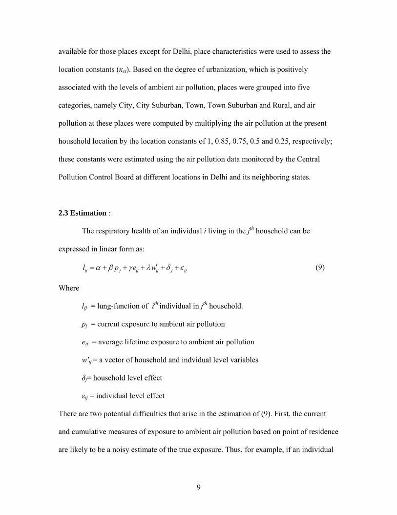
members of both households spend almost no time outside. Figures 5 and 6 provide

lowess estimates of the PM2.5 effects stratified by gender and economic status. While the

standard errors for the stratified estimates are too large to provide a compelling basis for

statistical inference the results correspond well to the time-allocation data. There is a

strong gradient in term of the male effects with poorer men exhibiting a significant

negative relationship between ambient air and respiratory health and better off men

exhibiting an insignificant relationship. On the other hand the relationship for women is

relatively flat and bordering on statistical insignificance throughout the range. .

5. CONCLUSION:

The results of this paper suggest that the changes in air quality regulations in

Delhi that have were put in place over the 1997-2002 period had a substantial effect on

respiratory health and that this effect was concentrated among low expenditure

households. The results appear to be robust to the possibility of endogenous residence but

importantly affected by treatment for measurement error. There are important limitations

to this analysis that may be addressed. First, we have constructed reduced form estimates

of the effects of ambient air quality. In particular, we have not considered the effects of

variation in indoor air quality or smoking that also may have important effects of lung

quality. To the extent that individuals and households alter these behaviors in response

16

exposure to ambient pollution we may be underestimating the direct effect of ambient air.

Second, while we have high-resolution estimates of current air quality our measurements

of lifetime exposure are imputed based on aggregate data. Obviously it is not possible, on

a retrospective basis, to collect the kind of detailed air quality data that was collected for

the post-regulation period. However, in ongoing work we are exploring the use of

MODIS satellite imagery to address this important limitation. While currently we are

limited from a technical standpoint to examining data at a resolution of 5km, the

evidence suggests that we can capture a substantial fraction of local variation in PM2.5 in

2003 using optical density compiled from the MODIS images. Application of these

methods to MODIS images from 2000 shows a slow negative trend as might be

anticipated using other available sources. To the extent that these methods may be used it

may be possible to get a much clearer sense of the overall impact of Delhi’s air quality

regulations on the health of her citizens. Finally, while it is not possible to obtain direct

estimates of respiratory health estimates prior to the introduction of the regulation

changes, it may be possible to use longitudinal data of this type to better control for the

cumulative effects of past exposure. A second round of this survey to collect additional

respiratory data is currently planned for 2007.

17

References:

Alberg AJ, Samet JM. 2003. Epidemiology of lung cancer. Chest 123(1): 21S-49S.

Brown P, Zavestoski S, Luebke T, Mandelbaum J, McCormick S, Mayer B. 2003. The

health politics of asthma: Environmental justice and collective illness experience in

the United States. Social Science and Medicine 57: 453-464.

Bell, Ruth Greenspan, Kuldeep Mathur, Urvashi Narain, and David Simpson, “Clearing

the Air: How Delhi Broke the Logjam on Air Quality Reforms”, Environment

Magazine, 46(3), April 2004.

Chay, Kenneth and Michael Greenstone, 2003, “Air Quality, Infant Mortality, and the

Clean Air Act of 1970,” NBER Working Paper 10053.

Chay, Kenneth, Carlos Dobkin and Michael Greenstone, 2003, “The Clean Air Act of

1970 and Adult Mortality,” (with), Journal of Risk and Uncertainty, 27(3): 279-300.

Chhabra SK, Chhabra P, Rajpal S, Gupta RK. 2001. Ambient air pollution and chronic

respiratory morbidity in Delhi. Arch Environ Health 56: 58-64.

Crapo RO, Morris AH, Gardner RM. 1981. Reference spirometric values using

techniques and equipment that meet ATS recommendations. Am. Rev. of Respir.

Dis. 123: 659-664.

Crapo RO, Morris AH. 1981. Standardized single-breath normal values for carbon

monoxide diffusing capacity. Am. Rev. of Respir. Dis. 123: 185-189.

Crapo RO, Morris AH, Clayton PD, Nixon CR. 1982. Lung volumes in healthy

nonsmoking adults. Bull. Europ. Physiopathol. Respir. 18: 419-425.

18

Cropper, M. L., N. B. Simon, A. Alberini, and P.K. Sharma, 1997. The Health Effects of

Air Pollution in Delhi, India. Policy Research Working Paper #1860, New York:

World Bank.

Dinda S. 2004. Environmental Kuznets curve hypothesis: A survey. Ecological

Economics 49(1), 431-455.

Dockery DW, Pope CA III. 1994. Acute respiratory effects of particulate air pollution.

Annual Review of Public Health 15: 107-32.

Government of India. 2005. White paper on pollution in Delhi with an action plan, New

Delhi. The Minister of Environment and Forests, Government of India.

URL: http://envfor.nic.in/divisions/cpoll/delpolln.html

Hertel O, Jensen SS, Berkowicz R, Brandt J, Christensen J. 2002. Modelling

concentrations of and human exposure to air pollution in Danish cities. In: Midgley,

P & Reuther M (eds.). Transport and chemical transformation in the troposphere.

Proceedings of EUROTRAC-2 Symposium.

Katsouyanni K, Touloumi G, Spix C, et al. 1997. Short-term effects of ambient sulphur

dioxide and particulate matter on mortality in 12 European cities: results from times

series data from the APHEA project. Air pollution and health: a European

approach. BMJ 314: 1658-63.

Marcotullio PJ, Williams E, Marshall JD. 2005. Faster, sooner, and more simultaneously:

How recent road and air transportation CO2 emission trends in developing countries

differ from historic trends in the United States. The Journal of Environment &

Development 14: 125-148.

19

Pande JN, Bhatta N, Biswas D, et al. 2001. Outdoor air pollution and emergency room

visits at a hospital in Delhi. Indian J Chest Dis Allied Sci 44: 13-19.

Pope AC, Thun MJ, Namboodir MM, et al. 1995. Particulate air pollution as a predictor

of mortality in a prospective study for US adults. American Journal of Respiratory

and Critical Care Medicine 151: 669-674.

Quanjer Ph H, Tammeling GJ, Cotes JE, et al. 1993. Lung volumes and forced

ventilatory flows. Eur Respir J 6(16): 5-40.

Ramachandran G, Adgate JL, Pratt GC, Sexton K. 2003. Characterizing indoor and

outdoor 15 minute average PM2.5 concentrations in urban neighborhoods. Aerosol

Science and Technology 37: 33-45.

Samet JM, Dominici F, Curriero FC, Coursac I, Zeger SL. 2000. Fine particulate air

pollution and mortality in 20 US cities, 1987-1994, The New England Journal of

Medicine 343(24): 1742-49.

Spengler JD, Treitman RD, Tosteson TD, Mage DT, Soczek ML. 1985. Personal

exposures to respirable particulates and implications of air pollution epidemiology.

Environ. Sci. Technol. 19(8): 700-707.

Schwartz J, Dockery DW, Neas LM. 1996. Is daily mortality associated specifically with

fine particles? J Air Waste Manag Assoc 46: 927-39.

TERI (Tata Energy Research Institute). 2001. Shut shop or shift base. Press release.

February.

TERI (Tata Energy Research Institute). 2001. Air quality in Delhi. Press release. August.

WHO, 2000. Guidelines for air quality, Geneva: World Health Organization.

20

Zidek JV, Shaddick G, White R, Meloche J, Chatfield C. 2005. Using a probabilistic

model (pCNEM) to estimate personal exposure to air pollution. Environmetrics 16:

481–493.

Table 1: Sources of Pollution in Delhi

Source 1970-71 1980-81 1990-91 2000-01 Industrial 56 40 29 20 Vehicular 23 42 64 72 Domestic 21 18 7 8

Source: Government of India, 1997

Table 2

Means and Standard Deviations by Residence

Total Inside Delhi Outside Delhi Different by location

Mean S.D. Mean S.D. Mean S.D. P-value Lung function 70.30 15.31 70.44 15.35 69.85 15.17 .287 Current PM2.5 35.31 4.14 34.14 4.06 38.95 1.37 .000 Av. Live PM2.5 38.14 10.35 39.86 10.43 32.78 7.99 .000 Pc Exp 1328 9523 1272 889 1501 1112 .000 Male .449 .497 .446 .497 .458 .499 .486 Age 3.122 18.25 31.20 18.32 31.30 18.03 .876 Duration of Residence 14.50 11.37 15.36 11.62 11.81 10.08 .000 N 4015 3040 975

Table 3

Estimates of the effects of current and estimated average lifetime PM2.5 exposure on lung function using household random and fixed effects

I Panel Estimates using

Exposure Variables

II I+ Variables and

Controls

III

II+Instruments for Measurement Error

IV III for PC

Expend<1224 Rs

V III for PC

Expend<1224 Rs

Random Effects

Fixed Effects

Random Effects

Fixed Effects

Random Effects

Fixed Effects

Random Effects

Fixed Effects

Random Effects

Fixed Effects

Current PM2.5a -0.152 -0.122 -1.023 -1.828 -0.298 (2.24)** (1.82)* (2.92)*** (2.85)*** -0.75 Av. Life M2.5a -0.076 -0.059 -0.059 -0.042 -0.628 -1.025 -0.67 -2.626 -0.261 0.34 (3.15)*** (1.75)* (2.48)** -1.28 (2.75)*** (1.89)* (2.27)** (1.71)* -0.88 -0.68 Log(PC Exp) 1.659 1.05 -2.271 0.673 (3.77)*** (2.04)** (1.4) (0.66) Male -2.258 -2.454 -2.375 -2.905 -1.177 -4.213 -3.144 -3.713 (4.83)*** (4.45)*** (4.65)*** (4.21)*** -1.45 (1.81)* (4.93)*** (4.75)***Age -0.348 -0.338 -0.188 -0.084 -0.25 0.253 -0.143 -0.263 (7.23)*** (5.75)*** (2.28)** -0.54 (1.75)* -0.55 -1.48 (1.75)* Age ^2 0.002 0.002 0 -0.001 0.001 -0.007 0 0.001 (3.55)*** (2.58)*** (0.21) (0.64) (0.51) (1.03) (0.11) (0.73) Constant 78.317 72.539 74.041 80.801 129.552 115.083 181.635 172.548 92.483 66.264 (29.23)*** 0 (17.44)*** 0 (5.99)*** (6.06)*** (4.55)*** (3.18)*** (3.76)*** (3.85)***People 3989 3989 3989 3989 3989 3989 1994 1994 1995 1995 Households 1550 1550 1550 1550 1550 1550 679 679 871 871 Random vs Fixed Effects

Χ2(1)=0.57 P=0.452

Χ2(4)=1.54 P=0.819

Χ2(4)=1.96 P=0.744

Χ2(4)=4.12 P=0.391

Χ2(1)=1.96 P=0.744

* significant at 10%; ** significant at 5%; *** significant at 1% a Treated for measurement error in specifications II-V, instruments are location, duration, and interaction.

Table 4

First stage estimates

PM2.5

Random Effects Average Lifetime PM2.5

Random Effects Average Lifetime PM2.5

Fixed Effects Log(Per Capita Expenditure (Rs)) -1.072 0.756 (6.61)*** (2.47)** Male -0.042 -0.464 -0.653 -0.36 -1.57 (1.92)* Age 0.003 0.247 0.235 -0.24 (8.17)*** (6.52)*** Age ^2 0 -0.004 -0.004 -0.01 (9.27)*** (7.19)*** Out of Delhi 5.307 -7.287 (20.29)*** (11.35)*** Duration in current residence 0.014 0.107 0.102 -1.29 (5.81)*** (3.33)*** Out of Delhi x Duration -0.026 0.033 -0.029 (1.96)* (0.9) (0.52) Constant 41.305 30.329 34.31 (35.04)*** (13.92)*** (54.87)*** Observations 4015 4015 4015 Number of group(H1) 0.27 1555 1555 R-squared 0.03

Test of excluded instruments Chi2(3) Χ2(3)= 253.51

P=.000

Χ2(3)= 316.43 P=.000

Χ2(2)= 6.05 P=.002

Absolute value of z statistics in parentheses * significant at 10%; ** significant at 5%; *** significant at 1%

Figure 1: Air quality sampling points and Interpolated estimates of PM2.5

Figure 2: Lowess estimates of effects of current exposure by PC expenditure

-2-1

.5-1

-.50

Effe

ct o

f exp

osur

e on

lung

func

tion

5 6 7 8 9Log(Per Capita Expenditure (Rs))

coef coef+secoef-se

Figure 3: Lowess Estimates of Effects of Average Lifetime Exposure by PC Expenditure

-1-.8

-.6-.4

-.20

Effe

ct o

f exp

osur

e on

lung

func

tion

5 6 7 8 9Log(Per Capita Expenditure (Rs))

coef coef+secoef-se

Figure 5 Estimates of time spent outside the household by sex and Per Capita Expenditure

02

46

8H

ours

per

day

5 6 7 8 9Log(Per Capita Expenditure (Rs))

Time spent outside (men) Time spent outside (w omen)

Figure 5 Lowess estimates of effects of current exposure by per capita expenditure for adult men

-2-1

0E

ffect

of e

xpos

ure

on lu

ng fu

nctio

n

5 6 7 8 9Log(Per Capita Expenditure (Rs))

coef coef+secoef-se

Figure 6 Lowess estimates of effects of current exposure by per capita expenditure for adult women

-2-1

0E

ffect

of e

xpos

ure

on lu

ng fu

nctio

n

5 6 7 8 9Log(Per Capita Expenditure (Rs))

coef coef+secoef-se