Embed Size (px)
Citation preview
Resurgence and the Physics of Divergence
Gerald Dunne
University of Connecticut
Young Theorists’ Forum, IPPP Durham, December 17, 2014
GD & M. Ünsal, 1210.2423, 1210.3646, 1306.4405, 1401.5202
GD, lectures at CERN 2014 Winter School
also with: G. Başar, A. Cherman, D. Dorigoni, R. Dabrowski: 1306.0921, 1308.0127,
1308.1108, 1405.0302
Physical Motivation
I strongly interacting/correlated systems
I non-perturbative definition of non-trivial QFT incontinuum
I analytic continuation of path integrals
I dynamical and non-equilibrium physics from path integrals
I uncover hidden ‘magic’ in perturbation theory
I “exact” asymptotics in QM, QFT and string theory
Physical Motivation
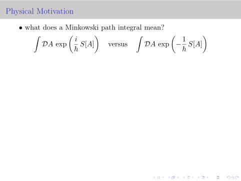
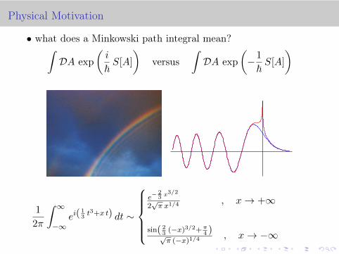
• what does a Minkowski path integral mean?∫DA exp
(i
~S[A]
)versus
∫DA exp
(−1
~S[A]
)
1
2π
∫ ∞
−∞ei(
13t3+x t) dt ∼
e−23 x
3/2
2√π x1/4
, x→ +∞
sin( 23
(−x)3/2+π4 )√
π (−x)1/4, x→ −∞
Physical Motivation
• what does a Minkowski path integral mean?∫DA exp
(i
~S[A]
)versus
∫DA exp
(−1
~S[A]
)
1
2π
∫ ∞
−∞ei(
13t3+x t) dt ∼
e−23 x
3/2
2√π x1/4
, x→ +∞
sin( 23
(−x)3/2+π4 )√
π (−x)1/4, x→ −∞
Mathematical Motivation
Resurgence: ‘new’ idea in mathematics (Écalle, 1980; Stokes, 1850)
resurgence = unification of perturbation theory andnon-perturbative physics
• perturbation theory generally ⇒ divergent series
• series expansion −→ trans-series expansion
• trans-series ‘well-defined under analytic continuation’
• perturbative and non-perturbative physics entwined
• applications: ODEs, PDEs, fluids, QM, Matrix Models, QFT,String Theory, ...
• philosophical shift:view semiclassical expansions as potentially exact

Trans-series
No function has yet presented itself in analysis, thelaws of whose increase, in so far as they can bestated at all, cannot be stated, so to say, inlogarithmico-exponential terms
G. H. Hardy, Divergent Series, 1949
• deep result: “this is all we need” (J. Écalle, 1980)
• trans-series in many physics applications:
f(g2) =
∞∑
n=0
∞∑
k=0
k−1∑
l=0
cn,k,l g2n
[exp
(− Sg2
)]k [log
(− 1
g2
)]l
• trans-monomials: g2, e−1g2 , ln(g2): familiar in physics

Resurgence
resurgent functions display at each of their singularpoints a behaviour closely related to their behaviourat the origin. Loosely speaking, these functionsresurrect, or surge up - in a slightly different guise,as it were - at their singularities
J. Écalle, 1980
n
m
• new: trans-series coefficients ck,l,p highly correlated• new: analytic continuation under control• new: exponentially improved asymptotics
Perturbation theory
• hard problem = easy problem + “small” correction
• perturbation theory generally → divergent series
e.g. QM ground state energy: E =∑∞
n=0 cn (coupling)n
I Zeeman: cn ∼ (−1)n (2n)!
I Stark: cn ∼ (2n)!
I cubic oscillator: cn ∼ Γ(n+ 12)
I quartic oscillator: cn ∼ (−1)nΓ(n+ 12)
I periodic Sine-Gordon (Mathieu) potential: cn ∼ n!
I double-well: cn ∼ n!
note generic factorial growth of perturbative coefficients
Perturbation theory
but it works ...
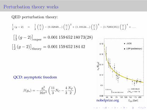
Perturbation theory works
QED perturbation theory:
1
2(g − 2) =
1
2
(α
π
)− (0.32848...)
(α
π
)2+ (1.18124...)
(α
π
)3− (1.7283(35))
(α
π
)4+ . . .
[12 (g − 2)
]exper
= 0.001 159 652 180 73(28)
[12 (g − 2)
]theory
= 0.001 159 652 184 42
QCD: asymptotic freedom
12
The left-hand panel shows a collection of different measurements by S. Bethke from High-
Energy International Conference in Quantum Chromodynamics, Montpellier 2002 (hep-
ex/0211012). The right-hand panel shows a collection by P. Zerwas, Eur. Phys. J.
C34(2004)41. JADE was one of the experiments at PETRA at DESY. NNLO means Next-to-
Next-to-Leading Order computation in QCD.
Although there are limits to the kind of calculations that can be performed to compare QCD
with experiments, there is still overwhelming evidence that it is the correct theory. Very
ingenious ways have been devised to test it and the data obtained, above all at the CERN LEP
accelerator, are bounteous. Wherever it can be checked, the agreement is better than 1%, often
much better, and the discrepancy is wholly due to the incomplete way in which the
calculations can be made.
The Standard Model for Particle Physics
QCD complemented the electro-weak theory in a natural way. This theory already contained
the quarks and it was natural to put all three interactions together into one model, a non-
abelian gauge field theory with the gauge group SU(3) x SU(2) x U(1). This model has been
called ‘The Standard Model for Particle Physics’. The theory explained the SLAC
experiments and also contained a possible explanation why quarks could not be seen as free
particles (quark confinement). The force between quarks grows with distance because of
‘infrared slavery’, and it is easy to believe that they are permanently bound together. There
are many indications in the theory that this is indeed the case, but no definite mathematical
proof has so far been advanced.
The Standard Model is also the natural starting point for more general theories that unify the
three different interactions into a model with one gauge group. Through spontaneous
symmetry breaking of some of the symmetries, the Standard Model can then emerge. Such
�(gs) = � g3s
16⇥2
�11
3NC � 4
3
NF
2
⇥
nobelprize.org
Perturbation theory
but it is divergent ...

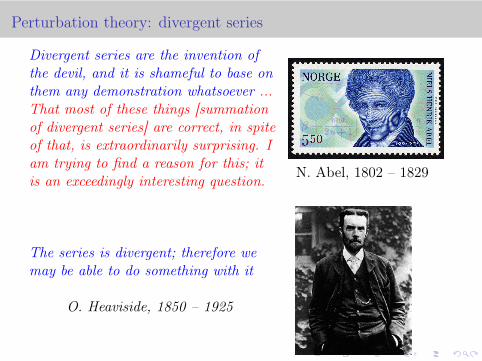
Perturbation theory: divergent series
Divergent series are the invention ofthe devil, and it is shameful to base onthem any demonstration whatsoever ...That most of these things [summationof divergent series] are correct, in spiteof that, is extraordinarily surprising. Iam trying to find a reason for this; itis an exceedingly interesting question. N. Abel, 1802 – 1829
The series is divergent; therefore wemay be able to do something with it
O. Heaviside, 1850 – 1925
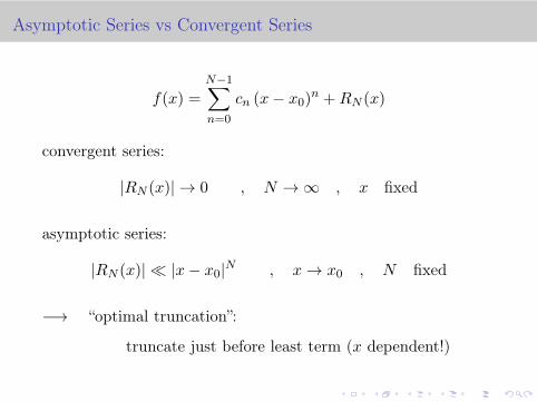
Asymptotic Series vs Convergent Series
f(x) =
N−1∑
n=0
cn (x− x0)n +RN (x)
convergent series:
|RN (x)| → 0 , N →∞ , x fixed
asymptotic series:
|RN (x)| � |x− x0|N , x→ x0 , N fixed
−→ “optimal truncation”:
truncate just before least term (x dependent!)
Asymptotic Series vs Convergent Series
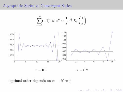
∞∑
n=0
(−1)n n!xn ∼ 1
xe
1x E1
(1
x
)
æ
æ
æ
æ
æ
æ
æ
æ
æ
æ
æ
æ
æ
æ
æ
æ
æ
æ æ æ
æ
0 5 10 15 20N
0.912
0.914
0.916
0.918
0.920
æ
æ
æ
æ
æ
æ
æ
æ
æ
æ
2 4 6 8 10N
0.75
0.80
0.85
0.90
0.95
1.00
1.05
1.10
x = 0.1 x = 0.2
optimal order depends on x: N ≈ 1x
Asymptotic Series: exponential precision
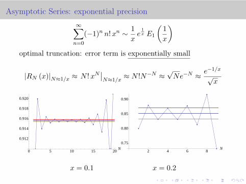
∞∑
n=0
(−1)n n!xn ∼ 1
xe
1x E1
(1
x
)
optimal truncation: error term is exponentially small
|RN (x)|N≈1/x ≈ N !xN∣∣N≈1/x
≈ N !N−N ≈√Ne−N ≈ e−1/x
√x
æ
æ
æ
æ
æ
æ
æ
æ
æ
æ
æ
æ
æ
æ
æ
æ
æ
æ æ æ
æ
0 5 10 15 20N
0.912
0.914
0.916
0.918
0.920
æ
æ
æ
æ
æ
æ
æ
æ
æ
2 4 6 8N
0.75
0.80
0.85
0.90
x = 0.1 x = 0.2

Asymptotic Series vs Convergent Series
Divergent series converge faster than convergentseries because they don’t have to converge
G. F. Carrier, 1918 – 2002
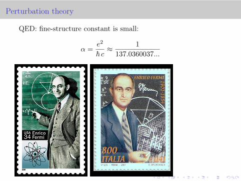
Perturbation theory
QED: fine-structure constant is small:
α =e2
~ c≈ 1
137.0360037...
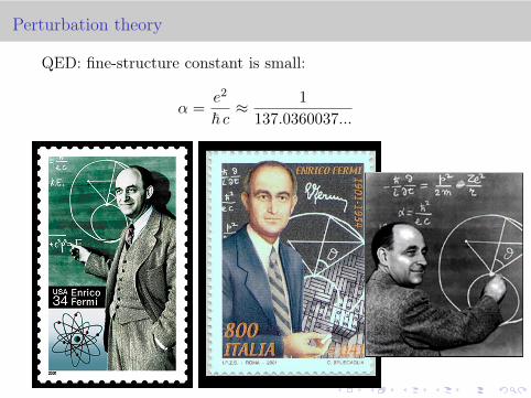
Perturbation theory
QED: fine-structure constant is small:
α =e2
~ c≈ 1
137.0360037...
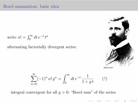
Borel summation: basic idea
write n! =∫∞
0 dt e−t tn
alternating factorially divergent series:
∞∑
n=0
(−1)n n! gn =
∫ ∞
0dt e−t
1
1 + g t(?)
integral convergent for all g > 0: “Borel sum” of the series
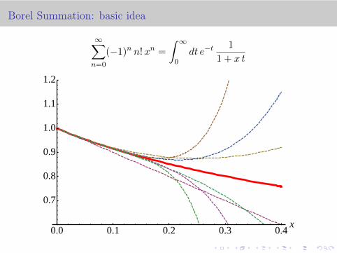
Borel Summation: basic idea
∞∑
n=0
(−1)n n!xn =
∫ ∞
0dt e−t
1
1 + x t
0.0 0.1 0.2 0.3 0.4x
0.7
0.8
0.9
1.0
1.1
1.2
Borel summation: basic idea
write n! =∫∞
0 dt e−t tn
non-alternating factorially divergent series:
∞∑
n=0
n! gn =
∫ ∞
0dt e−t
1
1− g t (??)
pole on the Borel axis!
⇒ non-perturbative imaginary part
± i πge− 1g
but every term in the series is real !?!
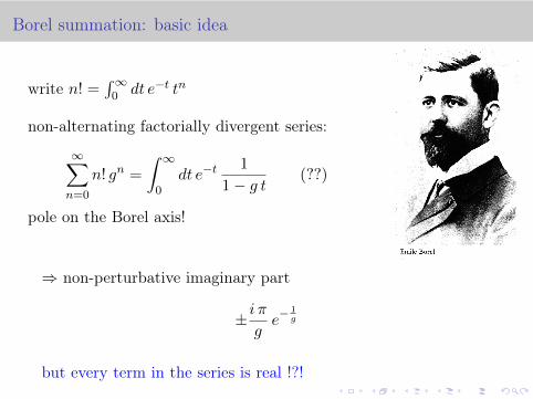
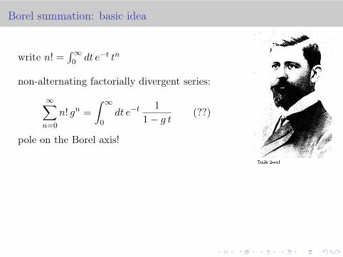
Borel summation: basic idea
write n! =∫∞
0 dt e−t tn
non-alternating factorially divergent series:
∞∑
n=0
n! gn =
∫ ∞
0dt e−t
1
1− g t (??)
pole on the Borel axis!
⇒ non-perturbative imaginary part
± i πge− 1g
but every term in the series is real !?!

Borel Summation: basic Idea
Borel ⇒ Re[ ∞∑
n=0
n!xn
]= P
∫ ∞
0dt e−t
1
1− x t =1
xe−
1x Ei
(1
x
)
0.5 1.0 1.5 2.0 2.5 3.0x
-0.5
0.5
1.0
1.5
2.0
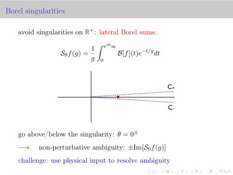
Borel singularities
avoid singularities on R+: lateral Borel sums:
Sθf(g) =1
g
∫ eiθ∞
0B[f ](t)e−t/gdt
C+
C-
go above/below the singularity: θ = 0±
−→ non-perturbative ambiguity: ±Im[S0f(g)]
challenge: use physical input to resolve ambiguity
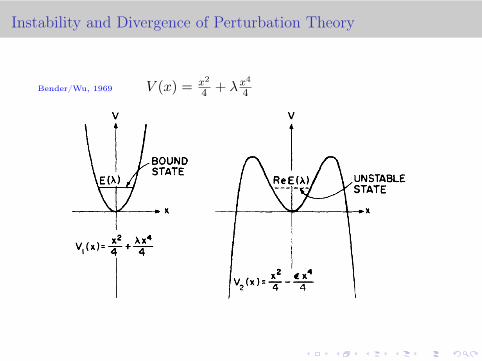
Instability and Divergence of Perturbation Theory
Bender/Wu, 1969 V (x) = x2
4 + λx4
4

Borel Summation and Dispersion Relations
cubic oscillator: V = x2 + λx3
A. Vainshtein, 1964
z= h2
. z o
C
R
E(z0) =1
2πi
∮
Cdz
E(z)
z − z0
=1
π
∫ R
0dz
ImE(z)
z − z0
=
∞∑
n=0
zn0
(1
π
∫ R
0dz
ImE(z)
zn+1
)
WKB ⇒ ImE(z) ∼ a√ze−b/z , z → 0
⇒ cn ∼a
π
∫ ∞
0dz
e−b/z
zn+3/2=a
π
Γ(n+ 12)
bn+1/2

Borel Summation and Dispersion Relations
cubic oscillator: V = x2 + λx3
A. Vainshtein, 1964
z= h2
. z o
C
R
E(z0) =1
2πi
∮
Cdz
E(z)
z − z0
=1
π
∫ R
0dz
ImE(z)
z − z0
=
∞∑
n=0
zn0
(1
π
∫ R
0dz
ImE(z)
zn+1
)
WKB ⇒ ImE(z) ∼ a√ze−b/z , z → 0
⇒ cn ∼a
π
∫ ∞
0dz
e−b/z
zn+3/2=a
π
Γ(n+ 12)
bn+1/2
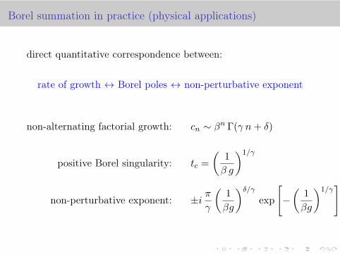
Borel summation in practice (physical applications)
direct quantitative correspondence between:
rate of growth ↔ Borel poles ↔ non-perturbative exponent
non-alternating factorial growth: cn ∼ βn Γ(γ n+ δ)
positive Borel singularity: tc =
(1
β g
)1/γ
non-perturbative exponent: ±i πγ
(1
βg
)δ/γexp
[−(
1
βg
)1/γ]
Divergence of perturbation theory
an important part of the story ...
The majority of nontrivial theories are seeminglyunstable at some phase of the coupling constant, whichleads to the asymptotic nature of the perturbative series
A. Vainshtein (1964)
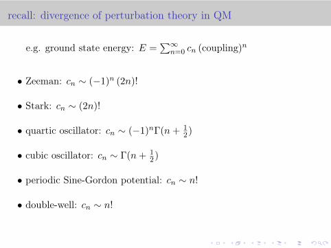
recall: divergence of perturbation theory in QM
e.g. ground state energy: E =∑∞
n=0 cn (coupling)n
• Zeeman: cn ∼ (−1)n (2n)!
• Stark: cn ∼ (2n)!
• quartic oscillator: cn ∼ (−1)nΓ(n+ 12)
• cubic oscillator: cn ∼ Γ(n+ 12)
• periodic Sine-Gordon potential: cn ∼ n!
• double-well: cn ∼ n!
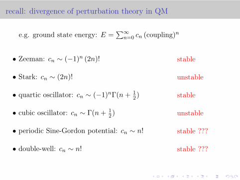
recall: divergence of perturbation theory in QM
e.g. ground state energy: E =∑∞
n=0 cn (coupling)n
• Zeeman: cn ∼ (−1)n (2n)!
• Stark: cn ∼ (2n)!
• quartic oscillator: cn ∼ (−1)nΓ(n+ 12)
• cubic oscillator: cn ∼ Γ(n+ 12)
• periodic Sine-Gordon potential: cn ∼ n!
• double-well: cn ∼ n!
stable
unstable
stable
unstable
stable ???
stable ???

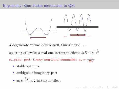
Bogomolny/Zinn-Justin mechanism in QM
... ...
• degenerate vacua: double-well, Sine-Gordon, ...
splitting of levels: a real one-instanton effect: ∆E ∼ e−Sg2
surprise: pert. theory non-Borel summable: cn ∼ n!(2S)n
I stable systems
I ambiguous imaginary part
I ±i e−2Sg2 , a 2-instanton effect
Bogomolny/Zinn-Justin mechanism in QM
... ...
• degenerate vacua: double-well, Sine-Gordon, ...
splitting of levels: a real one-instanton effect: ∆E ∼ e−Sg2
surprise: pert. theory non-Borel summable: cn ∼ n!(2S)n
I stable systems
I ambiguous imaginary part
I ±i e−2Sg2 , a 2-instanton effect
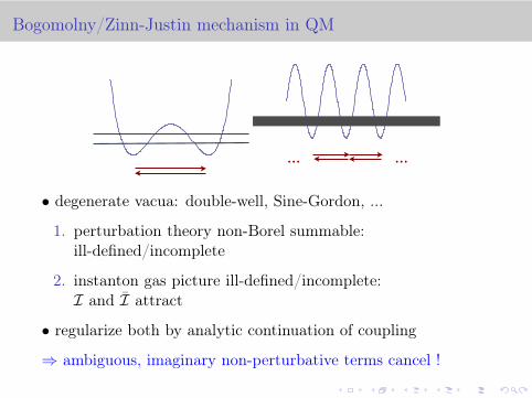
Bogomolny/Zinn-Justin mechanism in QM
... ...
• degenerate vacua: double-well, Sine-Gordon, ...
1. perturbation theory non-Borel summable:ill-defined/incomplete
2. instanton gas picture ill-defined/incomplete:I and I attract
• regularize both by analytic continuation of coupling
⇒ ambiguous, imaginary non-perturbative terms cancel !

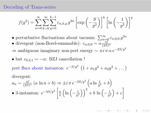
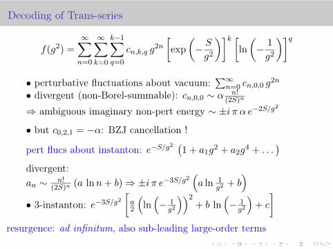
Decoding of Trans-series
f(g2) =
∞∑
n=0
∞∑
k=0
k−1∑
q=0
cn,k,q g2n
[exp
(− Sg2
)]k [ln
(− 1
g2
)]q
• perturbative fluctuations about vacuum:∑∞
n=0 cn,0,0 g2n
• divergent (non-Borel-summable): cn,0,0 ∼ α n!(2S)n
⇒ ambiguous imaginary non-pert energy ∼ ±i π α e−2S/g2
• but c0,2,1 = −α: BZJ cancellation !
pert flucs about instanton: e−S/g2(1 + a1g
2 + a2g4 + . . .
)
divergent:an ∼ n!
(2S)n (a lnn+ b)⇒ ±i π e−3S/g2(a ln 1
g2+ b)
• 3-instanton: e−3S/g2[a2
(ln(− 1g2
))2+ b ln
(− 1g2
)+ c
]
resurgence: ad infinitum, also sub-leading large-order terms
Towards Resurgence in QFT
• resurgence ≡ analytic continuation of trans-series
• effective actions, partition functions, ..., have natural integralrepresentations with resurgent asymptotic expansions
• analytic continuation of external parameters: temperature,chemical potential, external fields, ...
• e.g., magnetic ↔ electric; de Sitter ↔ anti de Sitter, . . .
• matrix models, large N , strings, ... (Mariño, Schiappa, ...)
• soluble QFT: Chern-Simons, ABJM, → matrix integrals
• asymptotically free QFT ?
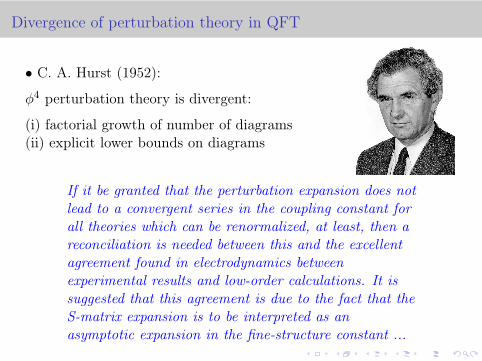
Divergence of perturbation theory in QFT
• C. A. Hurst (1952):φ4 perturbation theory is divergent:
(i) factorial growth of number of diagrams(ii) explicit lower bounds on diagrams
If it be granted that the perturbation expansion does notlead to a convergent series in the coupling constant forall theories which can be renormalized, at least, then areconciliation is needed between this and the excellentagreement found in electrodynamics betweenexperimental results and low-order calculations. It issuggested that this agreement is due to the fact that theS-matrix expansion is to be interpreted as anasymptotic expansion in the fine-structure constant ...
Dyson’s argument (QED)
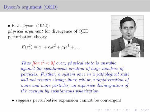
• F. J. Dyson (1952):physical argument for divergence of QEDperturbation theory
F (e2) = c0 + c2e2 + c4e
4 + . . .
Thus [for e2 < 0] every physical state is unstableagainst the spontaneous creation of large numbers ofparticles. Further, a system once in a pathological statewill not remain steady; there will be a rapid creation ofmore and more particles, an explosive disintegration ofthe vacuum by spontaneous polarization.
• suggests perturbative expansion cannot be convergent
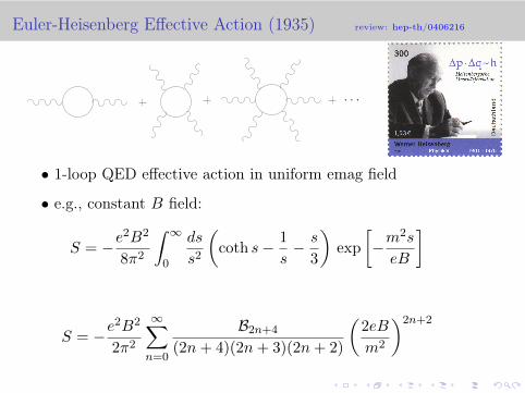
Euler-Heisenberg Effective Action (1935) review: hep-th/0406216
. . .
• 1-loop QED effective action in uniform emag field
• e.g., constant B field:
S = −e2B2
8π2
∫ ∞
0
ds
s2
(coth s− 1
s− s
3
)exp
[−m
2s
eB
]
S = −e2B2
2π2
∞∑
n=0
B2n+4
(2n+ 4)(2n+ 3)(2n+ 2)
(2eB
m2
)2n+2
Euler-Heisenberg Effective Action and Schwinger Effect
B field: QFT analogue of Zeeman effect
E field: QFT analogue of Stark effect
B2 → −E2: series becomes non-alternating
Borel summation ⇒ ImS = e2E2
8π3
∑∞k=1
1k2
exp[−km2π
eE
]
Schwinger effect:328 The European Physical Journal D
Fig. 1. Pair production as the separation of a virtual vacuumdipole pair under the influence of an external electric field.
asymptotic e+ e− pairs if they gain the binding energy of2mc2 from the external field, as depicted in Figure 1. Thisis a non-perturbative process, and the leading exponentialpart of the probability, assuming a constant electric field,was computed by Heisenberg and Euler [2,3]:
PHE ∼ exp
[−π m2 c3
e E !
], (3)
building on earlier work of Sauter [18]. This result sets abasic scale of a critical field strength and intensity nearwhich we expect to observe such nonperturbative effects:
Ec =m2c3
e !≈ 1016 V/cm
Ic =c
8πE2
c ≈ 4 × 1029 W/cm2. (4)
As a useful guiding analogy, recall Oppenheimer’s compu-tation [19] of the probability of ionization of an atom ofbinding energy Eb in such a uniform electric field:
Pionization ∼ exp
[−4
3
√2m E
3/2b
eE!
]. (5)
Taking as a representative atomic energy scale the binding
energy of hydrogen, Eb = me4
2!2 ≈ 13.6 eV, we find
P hydrogen ∼ exp
[−2
3
m2 e5
E !4
]. (6)
This result sets a basic scale of field strength and inten-sity near which we expect to observe such nonperturbativeionization effects in atomic systems:
E ionizationc =
m2e5
!4= α3Ec ≈ 4 × 10⁹ V/cm
I ionizationc = α6Ic ≈ 6 × 10¹⁶ W/cm2. (7)
These, indeed, are the familiar scales of atomic ioniza-tion experiments. Note that E ionization
c differs from Ec
by a factor of α3 ∼ 4 × 10⁻⁷. These simple estimatesexplain why vacuum pair production has not yet beenobserved – it is an astonishingly weak effect with con-ventional lasers [20,21]. This is because it is primarily anon-perturbative effect, that depends exponentially on the(inverse) electric field strength, and there is a factor of ∼107 difference between the critical field scales in the atomicregime and in the vacuum pair production regime. Thus,with standard lasers that can routinely probe ionization,there is no hope to see vacuum pair production. However,
recent technological advances in laser science, and also intheoretical refinements of the Heisenberg-Euler computa-tion, suggest that lasers such as those planned for ELImay be able to reach this elusive nonperturbative regime.This has the potential to open up an entirely new domainof experiments, with the prospect of fundamental discov-eries and practical applications, as are described in manytalks in this conference.
2 The QED effective action
In quantum field theory, the key object that encodes vac-uum polarization corrections to classical Maxwell electro-dynamics is the “effective action” Γ [A], which is a func-tional of the applied classical gauge field Aµ(x) [22–24].The effective action is the relativistic quantum field the-ory analogue of the grand potential of statistical physics,in the sense that it contains a wealth of information aboutthe quantum system: here, the nonlinear properties of thequantum vacuum. For example, the polarization tensor
Πµν = δ2ΓδAµδAν
contains the electric permittivity εij and
the magnetic permeability µij of the quantum vacuum,and is obtained by varying the effective action Γ [A] withrespect to the external probe Aµ(x). The general formal-ism for the QED effective action was developed in a se-ries of papers by Schwinger in the 1950’s [22,23]. Γ [A] isdefined [23] in terms of the vacuum-vacuum persistenceamplitude
〈0out | 0in〉 = exp
[i
!{Re(Γ ) + i Im(Γ )}
]. (8)
Note that Γ [A] has a real part that describes dispersive ef-fects such as vacuum birefringence, and an imaginary partthat describes absorptive effects, such as vacuum pair pro-duction. Dispersive effects are discussed in detail in Gies’scontribution to this volume [25]. The imaginary part en-codes the probability of vacuum pair production as
Pproduction = 1 − |〈0out | 0in〉|2
= 1 − exp
[−2
!Im Γ
]
≈ 2
!Im Γ (9)
here, in the last (approximate) step we use the fact thatIm(Γ )/! is typically very small. The expression (9) can beviewed as the relativistic quantum field theoretic analogueof the well-known quantum mechanical fact that the ion-ization probability is determined by the imaginary partof the energy of an atomic electron in an applied electricfield.
From a computational perspective, the effective actionis defined as [22–24]
Γ [A] = ! ln det [iD/ − m]
= ! tr ln [iD/ − m] . (10)
ImS → physical pair production rate
• suggests Euler-Heisenberg series must be divergent
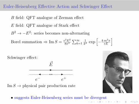
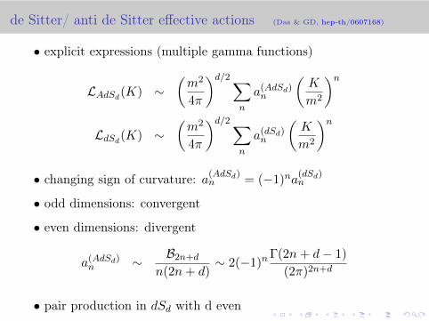
de Sitter/ anti de Sitter effective actions (Das & GD, hep-th/0607168)
• explicit expressions (multiple gamma functions)
LAdSd(K) ∼(m2
4π
)d/2∑
n
a(AdSd)n
(K
m2
)n
LdSd(K) ∼(m2
4π
)d/2∑
n
a(dSd)n
(K
m2
)n
• changing sign of curvature: a(AdSd)n = (−1)na
(dSd)n
• odd dimensions: convergent
• even dimensions: divergent
a(AdSd)n ∼ B2n+d
n(2n+ d)∼ 2(−1)n
Γ(2n+ d− 1)
(2π)2n+d
• pair production in dSd with d even
Resurgence and Analytic Continuation
another view of resurgence:
resurgence can be viewed as a method for making formalasymptotic expansions consistent with global analyticcontinuation properties
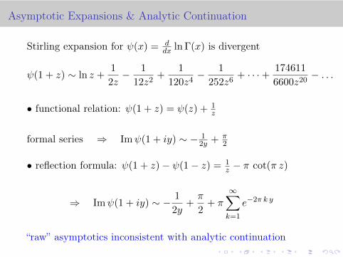
Asymptotic Expansions & Analytic Continuation
Stirling expansion for ψ(x) = ddx ln Γ(x) is divergent
ψ(1 + z) ∼ ln z +1
2z− 1
12z2+
1
120z4− 1
252z6+ · · ·+ 174611
6600z20− . . .
• functional relation: ψ(1 + z) = ψ(z) + 1z
formal series ⇒ Imψ(1 + iy) ∼ − 12y + π
2
• reflection formula: ψ(1 + z)− ψ(1− z) = 1z − π cot(π z)
⇒ Imψ(1 + iy) ∼ − 1
2y+π
2+ π
∞∑
k=1
e−2π k y
“raw” asymptotics inconsistent with analytic continuation
QFT: Renormalons
QM: divergence of perturbation theory due to factorial growthof number of Feynman diagrams
QFT: new physical effects occur, due to running of couplingswith momentum
• faster source of divergence: “renormalons”
• both positive and negative Borel poles

IR Renormalon Puzzle in Asymptotically Free QFT
perturbation theory: −→ ± i e−2Sβ0 g
2
instantons on R2 or R4: −→ ± i e−2Sg2
UV renormalon poles
instanton/anti-instanton poles
IR renormalon poles
appears that BZJ cancellation cannot occur
asymptotically free theories remain inconsistent’t Hooft, 1980; David, 1981
IR Renormalon Puzzle in Asymptotically Free QFT
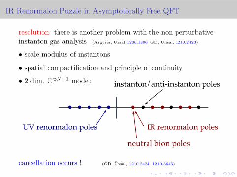
resolution: there is another problem with the non-perturbativeinstanton gas analysis (Argyres, Ünsal 1206.1890; GD, Ünsal, 1210.2423)
• scale modulus of instantons
• spatial compactification and principle of continuity
• 2 dim. CPN−1 model:
UV renormalon poles
instanton/anti-instanton poles
IR renormalon poles
neutral bion poles
cancellation occurs ! (GD, Ünsal, 1210.2423, 1210.3646)
The Bigger Picture
Q: should we expect resurgent behavior in QM and QFT ?
QM uniform WKB ⇒(i) trans-series structure is generic(ii) all multi-instanton effects encoded in perturbation theory(GD, Ünsal, 1306.4405, 1401.5202)
Q: what is behind this resurgent structure ?
• basic property of all-orders steepest descents integrals
Q: could this extend to (path) functional integrals ?
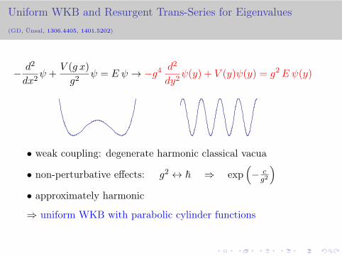
Uniform WKB and Resurgent Trans-Series for Eigenvalues(GD, Ünsal, 1306.4405, 1401.5202)
− d2
dx2ψ +
V (g x)
g2ψ = E ψ → −g4 d2
dy2ψ(y) + V (y)ψ(y) = g2E ψ(y)
• weak coupling: degenerate harmonic classical vacua
• non-perturbative effects: g2 ↔ ~ ⇒ exp(− cg2
)
• approximately harmonic
⇒ uniform WKB with parabolic cylinder functions
Connecting Perturbative and Non-Perturbative Sector
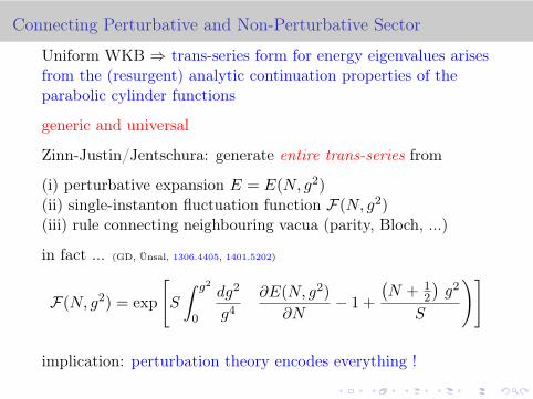
Uniform WKB ⇒ trans-series form for energy eigenvalues arisesfrom the (resurgent) analytic continuation properties of theparabolic cylinder functions
generic and universal
Zinn-Justin/Jentschura: generate entire trans-series from
(i) perturbative expansion E = E(N, g2)(ii) single-instanton fluctuation function F(N, g2)(iii) rule connecting neighbouring vacua (parity, Bloch, ...)
in fact ... (GD, Ünsal, 1306.4405, 1401.5202)
F(N, g2) = exp
[S
∫ g2
0
dg2
g4
(∂E(N, g2)
∂N− 1 +
(N + 1
2
)g2
S
)]
implication: perturbation theory encodes everything !
Connecting Perturbative and Non-Perturbative Sector
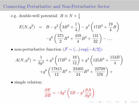
e.g. double-well potential: B ≡ N + 12
E(N, g2) = B − g2
(3B2 +
1
4
)− g4
(17B3 +
19
4B
)
−g6
(375
2B4 +
459
4B2 +
131
32
)− . . .
• non-perturbative function (F ∼ (...) exp[−A/2]):
A(N, g2) =1
3g2+ g2
(17B2 +
19
12
)+ g4
(125B3 +
153B
4
)
+g6
(17815
12B4 +
23405
24B2 +
22709
576
)+
• simple relation:
∂E
∂B= −3g2
(2B − g2 ∂A
∂g2
)
Connecting Perturbative and Non-Perturbative Sector
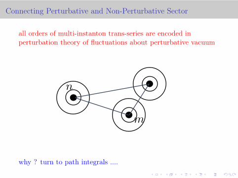
all orders of multi-instanton trans-series are encoded inperturbation theory of fluctuations about perturbative vacuum
n
m
why ? turn to path integrals ....
Analytic Continuation of Path Integrals
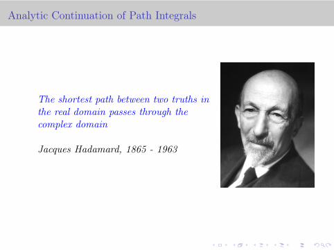
The shortest path between two truths inthe real domain passes through thecomplex domain
Jacques Hadamard, 1865 - 1963
All-Orders Steepest Descents: Darboux Theorem
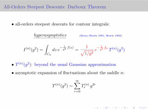
• all-orders steepest descents for contour integrals:
hyperasymptotics (Berry/Howls 1991, Howls 1992)
I(n)(g2) =
∫
Cn
dz e− 1g2f(z)
=1√1/g2
e− 1g2fn T (n)(g2)
• T (n)(g2): beyond the usual Gaussian approximation
• asymptotic expansion of fluctuations about the saddle n:
T (n)(g2) ∼∞∑
r=0
T (n)r g2r
All-Orders Steepest Descents: Darboux Theorem
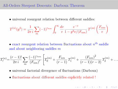
• universal resurgent relation between different saddles:
T (n)(g2) =1
2π i
∑
m
(−1)γnm∫ ∞
0
dv
v
e−v
1− g2v/(Fnm)T (m)
(Fnmv
)
• exact resurgent relation between fluctuations about nth saddleand about neighboring saddles m
T (n)r =
(r − 1)!
2π i
∑
m
(−1)γnm
(Fnm)r
[T
(m)0 +
Fnm(r − 1)
T(m)1 +
(Fnm)2
(r − 1)(r − 2)T
(m)2 + . . .
]
• universal factorial divergence of fluctuations (Darboux)
• fluctuations about different saddles explicitly related !
All-Orders Steepest Descents: Darboux Theorem
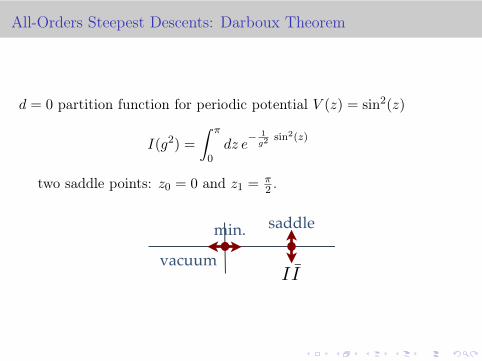
d = 0 partition function for periodic potential V (z) = sin2(z)
I(g2) =
∫ π
0dz e
− 1g2
sin2(z)
two saddle points: z0 = 0 and z1 = π2 .
IIvacuum vacuum
min. min.saddle
All-Orders Steepest Descents: Darboux Theorem
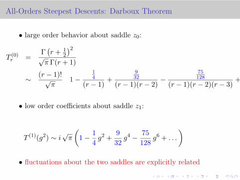
• large order behavior about saddle z0:
T (0)r =
Γ(r + 1
2
)2√π Γ(r + 1)
∼ (r − 1)!√π
(1−
14
(r − 1)+
932
(r − 1)(r − 2)−
75128
(r − 1)(r − 2)(r − 3)+ . . .
)
• low order coefficients about saddle z1:
T (1)(g2) ∼ i√π(
1− 1
4g2 +
9
32g4 − 75
128g6 + . . .
)
• fluctuations about the two saddles are explicitly related

Resurgence in Path Integrals: “Functional Darboux Theorem”
could something like this work for path integrals?
“functional Darboux theorem” ?
• multi-dimensional case is already non-trivial and interestingPham (1965); Delabaere/Howls (2002)
• Picard-Lefschetz theory
• do a computation to see what happens ...
Resurgence in Path Integrals
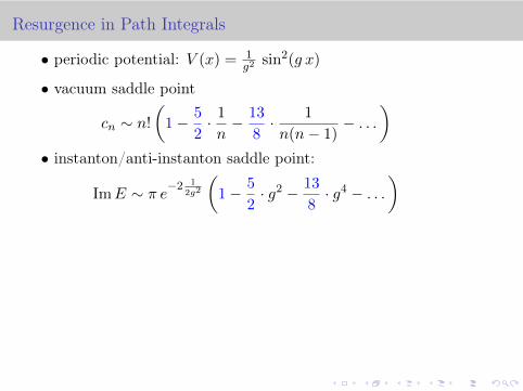
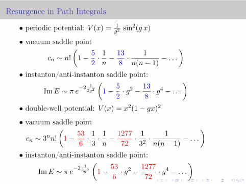
• periodic potential: V (x) = 1g2
sin2(g x)
• vacuum saddle point
cn ∼ n!
(1− 5
2· 1
n− 13
8· 1
n(n− 1)− . . .
)
• instanton/anti-instanton saddle point:
ImE ∼ π e−2 12g2
(1− 5
2· g2 − 13
8· g4 − . . .
)
• double-well potential: V (x) = x2(1− gx)2
• vacuum saddle point
cn ∼ 3nn!
(1− 53
6· 1
3· 1
n− 1277
72· 1
32· 1
n(n− 1)− . . .
)
• instanton/anti-instanton saddle point:
ImE ∼ π e−2 16g2
(1− 53
6· g2 − 1277
72· g4 − . . .
)
Resurgence in Path Integrals
• periodic potential: V (x) = 1g2
sin2(g x)
• vacuum saddle point
cn ∼ n!
(1− 5
2· 1
n− 13
8· 1
n(n− 1)− . . .
)
• instanton/anti-instanton saddle point:
ImE ∼ π e−2 12g2
(1− 5
2· g2 − 13
8· g4 − . . .
)
• double-well potential: V (x) = x2(1− gx)2
• vacuum saddle point
cn ∼ 3nn!
(1− 53
6· 1
3· 1
n− 1277
72· 1
32· 1
n(n− 1)− . . .
)
• instanton/anti-instanton saddle point:
ImE ∼ π e−2 16g2
(1− 53
6· g2 − 1277
72· g4 − . . .
)
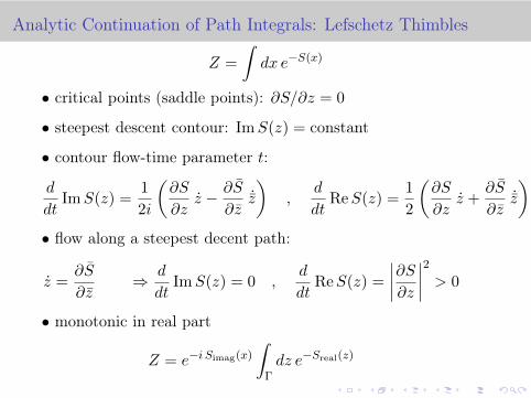
Analytic Continuation of Path Integrals: Lefschetz Thimbles
Z =
∫dx e−S(x)
• critical points (saddle points): ∂S/∂z = 0
• steepest descent contour: ImS(z) = constant
• contour flow-time parameter t:
d
dtImS(z) =
1
2i
(∂S
∂zz − ∂S
∂z˙z
),
d
dtReS(z) =
1
2
(∂S
∂zz +
∂S
∂z˙z
)
• flow along a steepest decent path:
z =∂S
∂z⇒ d
dtImS(z) = 0 ,
d
dtReS(z) =
∣∣∣∣∂S
∂z
∣∣∣∣2
> 0
• monotonic in real part
Z = e−i Simag(x)
∫
Γdz e−Sreal(z)
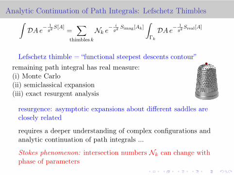
Analytic Continuation of Path Integrals: Lefschetz Thimbles∫DAe−
1g2S[A]
=∑
thimbles k
Nk e−ig2Simag[Ak]
∫
Γk
DAe−1g2Sreal[A]
Lefschetz thimble = “functional steepest descents contour”remaining path integral has real measure:(i) Monte Carlo(ii) semiclassical expansion(iii) exact resurgent analysis
resurgence: asymptotic expansions about different saddles areclosely related
requires a deeper understanding of complex configurations andanalytic continuation of path integrals ...
Stokes phenomenon: intersection numbers Nk can change withphase of parameters
Non-perturbative Physics Without Instantons
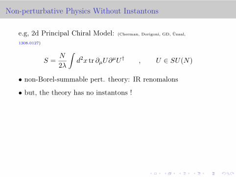
e.g, 2d Principal Chiral Model: (Cherman, Dorigoni, GD, Ünsal,
1308.0127)
S =N
2λ
∫d2x tr ∂µU∂
µU † , U ∈ SU(N)
• non-Borel-summable pert. theory: IR renomalons
• but, the theory has no instantons !
resolution: non-BPS saddle point solutions to 2nd-orderclassical Euclidean equations of motion: “unitons”
∂µ
(U †∂µ U
)= 0 (Uhlenbeck 1985)
• have negative fluctuation modes: saddles, not minima
• fractionalize on cylinder −→ BZJ cancellation
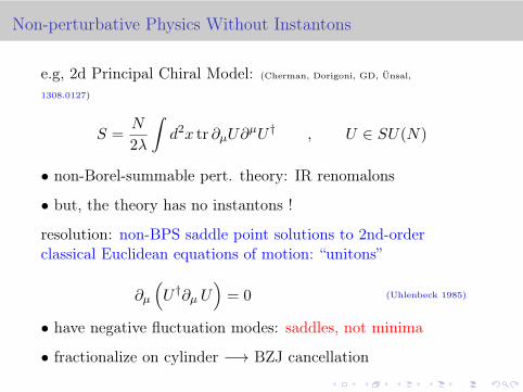
Non-perturbative Physics Without Instantons
e.g, 2d Principal Chiral Model: (Cherman, Dorigoni, GD, Ünsal,
1308.0127)
S =N
2λ
∫d2x tr ∂µU∂
µU † , U ∈ SU(N)
• non-Borel-summable pert. theory: IR renomalons
• but, the theory has no instantons !
resolution: non-BPS saddle point solutions to 2nd-orderclassical Euclidean equations of motion: “unitons”
∂µ
(U †∂µ U
)= 0 (Uhlenbeck 1985)
• have negative fluctuation modes: saddles, not minima
• fractionalize on cylinder −→ BZJ cancellation
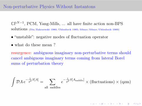
Non-perturbative Physics Without Instantons
CPN−1, PCM, Yang-Mills, ... all have finite action non-BPSsolutions (Din/Zakrzewski 1980; Uhlenbeck 1985; Sibner/Sibner/Uhlenbeck 1989)
• “unstable”: negative modes of fluctuation operator
• what do these mean ?
resurgence: ambiguous imaginary non-perturbative terms shouldcancel ambiguous imaginary terms coming from lateral Borelsums of perturbation theory
∫DAe−
1g2S[A]
=∑
all saddles
e− 1g2S[Asaddle] × (fluctuations)× (qzm)

Non-perturbative Physics Without Instantons: CPN−1
(Dabrowski, GD, arXiv:1306.0921)

Conclusions
• perturbation theory is generically divergent
• resurgence systematically unifies perturbation theory andnon-perturbative physics into a trans-series
• there is extra ‘magic’ in perturbation theory
• IR renormalon puzzle in asymptotically free QFT
• basic property of steepest descents expansions
• moral: consider all saddles, including non-BPS
• resurgence required for analytic continuation
Open Problems
• natural path integral construction
• analytic continuation of path integrals
• physics of QFT saddles/thimbles ?
• renormalization group flow ?
• strong- & weak-coupling expansions: dualities ?
• operator product expansion (OPE) ?
• SUSY and extended SUSY ?
• localization ?
• . . .
![RESURGENCE in Quasiclassical Scattering Richard E. Prange Department of Physics, University of Maryland [Work done at MPIPKS, Dresden] Thanks to Peter](https://img.pdfslide.net/doc/110x75/56649d3a5503460f94a158fd/resurgence-in-quasiclassical-scattering-richard-e-prange-department-of-physics.jpg)