Retirement and the Marginal Utility of Income

Andrew E. Clark

Paris School of Economics - CNRS

Yarine Fawaz

Universitat Autonoma de Barcelona

Abstract

Subjective well-being (SWB) has been shown to be a strong predictor of future

outcomes, whether on the labour market (e.g job quits, unemployment duration) or

in other domains of life (e.g marital break ups). In order to overcome the issue of

heterogeneity in SWB functions, empirical work has introduced individual-speci�c

e�ects into well-being regressions. However, this latter only addresses �level hetero-

geneity�. If SWB functions are interpersonally comparable, then their slopes with

respect to the variables of interest will also a�ect behaviour. We here appeal to

latent-class analysis to model both intercept and slope heterogeneity in SWB, and

then evaluate the impact these slopes on transitions to retirement. We identify sev-

eral groups of individuals whose SWB is not a�ected in the same way by income.

We use this slope heterogeneity to construct a continuous measure of the marginal

utility of income. When we estimate retirement probability as a function of this

income elasticity of well-being, we �nd that the more individuals value a unit of

income, the less likely they will retire. This correlation is found conditional on both

the level of income and the level of well-being.

Keywords: Subjective Well-being, Retirement, Marginal Utility of Income, Latent

Class Models.

JEL classi�cation: I31, C35.

Acknowledgements We would like to thank Jérôme Adda, Didier Blanchet, Partha

Deb, Richard Disney, and participants at the OECD Conference on �New Directions in

1

Welfare� (Paris), the Royal Economic Society Annual Conference (Cambridge), the Span-

ish Economic Association Conference (Vigo), the HEIRS Public Happiness Conference

(Rome), and the EALE Conference (Torino) for helpful comments. This research uses

data from RAND HRS Data, Version I, produced by the RAND Center for the Study

of Aging, with funding from the National Institute on Aging and the Social Security

Administration. Santa Monica, CA.

2

1 Introduction

While the retirement decision has been at the heart of much work across OECD countries,

it has essentially concentrated on the �objective� characteristics inducing older individuals

to retire, with far less being known about the relationship between subjective well-being

and retirement. Most of the literature dealing with well-being and retirement has focused

on the e�ect of retirement on life satisfaction (Wottiez and Theeuwes [1998]; Kim and

Moen [June 2001]; Lindeboom, Portrait, and van den Berg [2002]; Charles [2004]; Borsch-

Supan and Jurges [2007]; Seitsamo [2007]; Bonsang and Klein [2011]). With pension

systems needing to be re-designed to become sustainable, and the preferred option in

many countries consisting in increasing the legal retirement age, the e�ects of retiring on

subjective well-being are of great interest for policymakers. In a very similar vein, other

work has examined retirement satisfaction. Shultz, Morton, and Weckerle [1998] consider

the relative importance of �push� (e.g. poor health) and �pull� (e.g. leisure) factors

on retirement satisfaction, Elder and Rudolph [1999] investigate the role of �nancial

planning and expectations, Panis [2004] relates annuities and wealth to both retirement

satisfaction and measures of depression, and Bender [2004] emphasises the non-economic

determinants of well-being in retirement. However, although well-being has been shown

to predict future behaviour, it has rarely been considered in the context of retirement (an

exception is Debrand and Sirven [2009], who con�rm a negative impact of job satisfaction

on retirement).

In this paper we estimate the impact of well-being on retirement using the Health

and Retirement Study (HRS), and explicitly allow for slope heterogeneity across (latent)

groups of individuals. We appeal to a �nite mixture model (FMM) with panel data to

model heterogeneity in the marginal utility of income, and then see whether this marginal

utility of income a�ects retirement. The data identify two latent classes of individuals in

terms of the relationship between well-being and income. The model strongly rejects the

hypothesis of an equal e�ect of income on well-being across these two groups. We use the

estimated slopes and individual group membership probabilities to construct a continuous

measure of the marginal utility of income. We then estimate retirement probability as a

function of this elasticity of well-being to income.

We add to the existing literature on well-being and retirement in a number of ways.

First, we introduce heterogeneity into the income to well-being relationship. This allows

3

us to explore the determinants of class membership. Our results suggest that �money

buys happiness� much more for one group than for another, and also provide us with

information about �for whom it buys the most happiness�. Last, our retirement model

suggests a signi�cant negative e�ect of this estimated marginal utility of income: those

who value their income the least are more likely to retire. We can then encourage labour-

force participation via income measures for those who are most �income-sensitive�, but

much less so for the other groups. Finding that the slope of the estimated well-being

function predicts future behaviour is also a new �nding in the empirical literature on the

validation of Subjective Well-Being (SWB) measures.

The remainder of the paper is organised as follows. In the next section, we provide

a brief overview of the existing literature on the marginal utility of income. Section 3

then describes the data and the initial results, and Section 4 explains the econometric

methodology. In Section 5 we present our results and answer the question of the impact

of the marginal utility of income on the retirement probability. Last, Section 6 concludes.

2 The Marginal Utility of Income

The impact of the marginal utility of income on retirement is at the heart of the current

paper. As such, our �rst step is to estimate this marginal utility of income. We will

here use subjective well-being scores as proxy measures of utility. By doing so, we are

not measuring ex ante decision utility but rather ex post experienced utility (Kahneman,

Wakker, and Sarin [1997]). One suspicion amongst economists is that what individuals

say may not always reveal their preferences (and thus their behaviour). A valid response

to this suspicion is to note the literature in which cross-section distributions of well-

being predict individual future behaviour in panel data. The underlying idea here is that

individuals can be shown to to discontinue activities associated with lower well-being

levels (see Kahneman, Fredrickson, Schreiber, and Redelmeier [1993]; Frijters [2000]; Shiv

and Huber [2000]). An example of such work is job satisfaction predicting future job quits,

even when controlling for wages, hours of work and other standard individual and job

variables (see, amongst others, Freeman [1978]; Clark, Georgellis, and Sanfey [1998]; Clark

[2001]; Kristensen and Westergaard-Nielsen [2006]). A recent example using data on the

self-employed is found in Georgellis, Sessions, and Tsitsianis [2007]. Clark [2003] shows

that mental stress scores on entering unemployment predict unemployment duration:

4

those who su�ered the sharpest drop in well-being upon entering unemployment were the

quickest to leave it. Further, Ia�aldano and Muchinsky [1985] and Ostro� [1992] report

that higher job satisfaction within a �rm is positively correlated with its performance.

Equally, Rogers, Clow, and Kash [1994] �nd that job satisfaction is also correlated with

increased customer satisfaction within service industries. This predictive power is also

found in other domains. Life satisfaction predicts marital break-up (Guven, Senik, and

Stichnoth [2012]), as well as future morbidity and mortality. This literature shows that

individual subjective well-being scores are at least partly interpersonally comparable,

otherwise they would not be able to predict future individual behaviour and outcomes.

We then use self-reported SWB as a proxy for utility, and appeal to the relation

between the former and income to provide an estimate of the marginal utility of income.

There does still remain the issue of the interpretation of reported satisfaction scores. As

stated in Senik [2005],

interpreting subjective satisfaction data implies (i) relating discrete verbal

satisfaction judgements to a latent, unobserved, continuous utility variable,

and (ii) associating utility levels to observable characteristics. At each stage

of this process, strong assumptions must be accepted: (a) the link between

observable variables (income for instance) and latent utility is the same for

all individuals, i.e. the parameters of the individual satisfaction function

are identical for all agents (Tinbergen [1991]), (b) the association between a

verbal satisfaction label and a latent utility level is the same for everybody. If

either of these two assumptions is not veri�ed, any interpretation of reported

satisfaction will be misleading because of an �anchoring e�ect� (Winkelmann

and Winkelmann [1998]).

The traditional approach to dealing with unobserved heterogeneity is the use of individual-

speci�c �xed e�ects (see Clark and Oswald [2002]; Ferrer-i Carbonell and Frijters [2004];

Senik [2004]).

The development of �nite mixture models in the statistical literature in the 1960s

and 1970s, is an alternative way of capturing unobserved heterogeneity. The underlying

idea in these models is that the unknown population distribution may be empirically

approximated by a mixture of distributions with a �nite number of components. The

path-breaking work on the expectations-maximization (EM) algorithm (by Dempster,

Laird and Rubin [1977] and Aitkin and Rubin [1985]) made the computation of the

5

latent class models accessible to applied researchers. In recent years, the �nite mixture

model has found many applications, e.g. in Eckstein and Wolpin [1999]; Thacher and

Morey [2003], and the work of Deb who has contributed a great to render these models

attractive (see Deb and Trivedi [1997]; Ayyagari, Deb, Fletcher, Gallo, and Sindelar [2009];

Deb, Gallo, Ayyagari, Fletcher, and Sindelar [2009]). Clark, Etilé, Postel-Vinay, Senik,

and Van Der Straeten [2005] model intercept and slope heterogeneity using latent class

techniques to allow the parameters of the unobserved individual utility function to di�er

across individuals. In this paper we follow the same approach consisting in letting the

data speak. Our data here identify two classes of individuals, and strongly reject the

hypothesis that the marginal e�ect of income on well-being is identical across classes.

The use of individual �xed e�ects (intercept heterogeneity) therefore seems insu�cient,

and we need to also consider slope heterogeneity.

Last, in the existing SWB literature marginal utility is traditionally estimated (taking

unobserved heterogeneity into account or not) conditional on a wide range of other right-

hand side variables (common ones are gender, marital and labour-force status, health,

education, etc.). This therefore misses out the indirect e�ects of the variable of interest

here (income) on utility. Income is commonly-believed to have a positive e�ect on health,

for example. And health and SWB are positively correlated (see Dolan, Fujiwara, and

Metcalfe [2011]). We want to establish the overall impact of income on utility, including

any indirect e�ects of income via other right-hand side variables. When we estimate

the marginal utility of income using FMM, we �rst regress SWB on income only with

no other explanatory variables. As a speci�cation check (but aware that this may bias

the estimated coe�cient on income), we include a number of di�erent sets of additional

control variables in the SWB equation.

3 Data and Initial Results

3.1 Data

We use data from the Health and Retirement Study (HRS), which is a nationally-

representative longitudinal survey of individuals aged over 50 and their spouses. In the

�rst interview in 1992, HRS participants included 12,652 individuals from 7,702 house-

holds. The HRS initially sampled persons in birth cohorts 1931 through 1941 in 1992,

with follow-up interviews every two years. In 1998, people from the 1924 to 1930 and

6

1942 to 1947 cohorts were added to the original sample; and in 2004 it was the turn of in-

dividuals from the 1948 to 1953 cohort. Our analysis here uses data from Version I of the

data prepared by RAND, which is a cleaned and processed version of the HRS data. As

of today, these data are made of 10 waves from 1992 to 2010, of which we use waves 2 to

8, i.e. from year 1994 to 2006. As explained below, our measure of subjective well-being

has been incorporated from wave 2 on, leading us to discarding wave 1. We chose not to

use the last two waves for the job occupation variables were recoded in a way that allows

no direct equivalence. Up to 2006 the 1980 SOCs (Standard Occupational Codes) were

collapsed into 17 categories following a hierarchical structure taking into account knowl-

edge, skill level and experience. From year 2008 (waves 9 and 10), on the other hand, the

2000 SOCs have been collapsed into 25 categories, which are grouped according to �job

families�. The general concept behind this new classi�cation consists in combining people

who work together producing the same kinds of goods and services regardless of their skill

level, for example doctors, nurses, and health technicians. In addition, the 2000 SOCs

have more professional, technical, and service occupations and fewer production and ad-

ministrative support occupations, which makes it more di�cult to build an equivalence

between the two classi�cations. Although a � `crosswalk� was created in this very purpose,

it only concerns the management/professional category.

The RAND-HRS data have included an abridged version of the Center for Epidemi-

ologic Studies-Depression (CESD) Scale (Radlo� [1977]) since wave 2. The CESD de-

pression scale originally comprised twenty items. The HRS only retains eight of them:

depressive feelings, everything seen as an e�ort, restless sleep, could not get going, lone-

liness, sadness, enjoyment, happiness. All the questions asked to derive the CESD score

are Yes/No indicators of the respondent's feelings much of the time over the week prior

to the interview. The between-item validity of the CESD scale (Cronbach's alpha = 0.72)

is su�ciently high for the well-being measure to be considered as robust. The resulting

depression score is the number of questions to which the individual replies positively for

the �rst six items, and negatively for the last two. We then reverse this depression score

to produce a SWB scale where 0 indicates the worst level of psychological wellbeing and

8 the best.

Tables 3 and 4 in the appendix present information about our estimation sample. We

consider all individuals who were working at the time of the interview. This produces

36,283 observations (on 11,719 individuals) for whom we have non-missing information,

7

over the last seven waves of the HRS. We note that the sample statistics appear reasonable

and fall within expectations. In addition to the usual socio-demographic and economic

variables (gender, marital status, number of children, age, education, race, health status,

total household wealth, total household income) and job-related variables (number of

hours worked, occupation), two subjective variables are worth emphasising. One is on

risk aversion, on a scale from 1 to 4, where 1 indicates the least risk-averse preferences.

This variable is based on a series of �income gamble� questions: it is coded 1 if the

respondent would take a job with even chances of doubling or halving income; 2 for a

job with even chances of doubling income or cutting it by a third; 3 for a job with even

chances of doubling income or cutting it by 20%; and 4 if he would take or stay in a job

that guaranteed current income given any of the above alternatives. As these questions

were not asked in the 1994 and 1996 waves of the HRS, nor in the interviews by proxy,

we replace missing values with data from the closest past wave for every individual. If

the individual answered these questions at a number of di�erent waves, we take the mean

answer. The sample size falls with the inclusion of the risk-aversion variable. Most of our

sample is risk-averse, with 60% giving the most risk-averse answers and only 12% the most

risk-loving answer. We take the same �imputation� approach for the �nancial planning

horizon variable. Individuals are asked �In deciding how much of your (family) income

to spend or save, people are likely to think about di�erent �nancial planning periods. In

planning your (family's) savings and expenditure, which of the time periods listed in the

booklet is most important to you [and your husband/wife/partner]?�. Our measure of

planning behaviour is coded 1 if their answer is �next few months�, 2 corresponds to �next

year�, 3 to �next few years�, 4 to �next 5-10 years�, and 5 to �longer than 10 years�. Most

individuals declare thinking in terms of the next few years or next 5 to 10 years, which

are intermediate answers.

The SWB distribution is shown in Table 5. This is largely right-skewed, with over

75 per cent of the pooled sample reporting scores of 7 or 8, and less than 1 per cent a

zero score. The �between� distribution con�rms the prevalence of high scores of SWB as

over 70 per cent of the individuals recorded an 8 score at least once while less than 2

per cent have given a zero score. �Within� individuals (see last column), 73 per cent of

those who ever reported a score of 8 remained at that level. On the contrary only 44 per

cent of the individuals who gave a score of zero gave it at every wave. This either re�ects

measurement error, or that most people who reported low scores had indeed had a bad

8

year, and had better years in other waves.

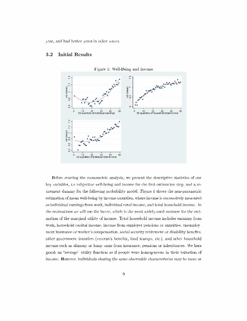
3.2 Initial Results

Figure 1: Well-Being and Income

Before starting the econometric analysis, we present the descriptive statistics of our

key variables, i.e subjective well-being and income for the �rst estimation step, and a re-

tirement dummy for the following probability model. Figure 1 shows the non-parametric

estimation of mean well-being by income quantiles, where income is successively measured

as individual earnings from work, individual total income, and total household income. In

the estimations we will use the latter, which is the most widely-used measure for the esti-

mation of the marginal utility of income. Total household income includes earnings from

work, household capital income, income from employer pensions or annuities, unemploy-

ment insurance or worker's compensation, social security retirement or disability bene�ts,

other government transfers (veteran's bene�ts, food stamps, etc.), and other household

income such as alimony or lump sums from insurance, pensions or inheritances. We here

graph an �average� utility function as if people were homogeneous in their valuation of

income. However, individuals sharing the same observable characteristics may be more or

9

less happy depending on what we might call their �personality� type. Self-determination

theory (see [Ryan and Deci, 2000]) suggests that behaviour can be intrinsically or ex-

trinsically motivated. An internally-motivated individual derives much more utility from

social interactions and community involvement than from accumulating wealth, while the

extrinsically motivated derive their utility from income gains. Individuals may also be

heterogeneous in the way they translate their latent unobserved utility into a discrete

verbal satisfaction answer. Depending on interactions with the surveyor, mood e�ects, or

question formulation, there is room for heterogeneity in their response. Our FMM analy-

sis allows the relationship between income and well-being to di�er between individuals in

terms of both the intercept and the slope. We will use the panel dimension of the HRS,

and separate the time-series and cross-sectional information it provides, i.e. �between�

movements (between distinct subjects) and �within� movements (panel information for

one subject). We expect to �nd a great deal of heterogeneity between individuals, as

their heterogeneous valuations of income might depend on their personality, but much

less variation within individuals at di�erent points in time. This method does not allow

the two potential sources of heterogeneity (in the utility function and in the reports of

utility) to be disentangled though.

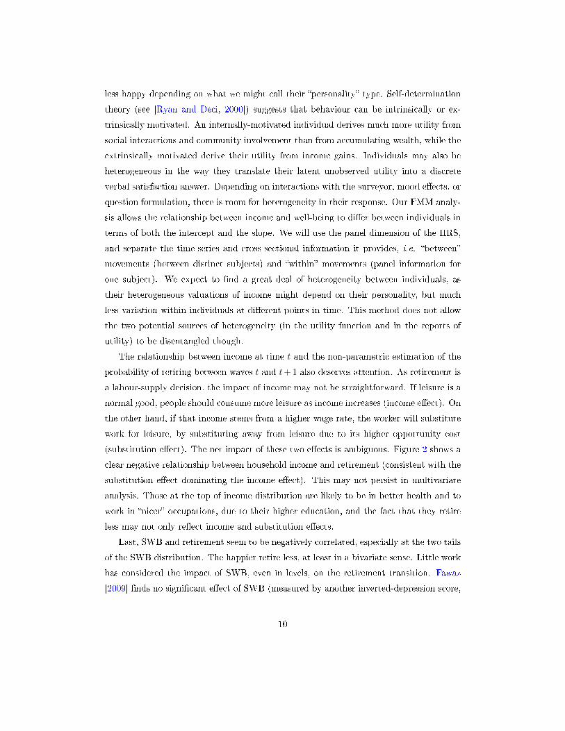
The relationship between income at time t and the non-parametric estimation of the

probability of retiring between waves t and t+ 1 also deserves attention. As retirement is

a labour-supply decision, the impact of income may not be straightforward. If leisure is a

normal good, people should consume more leisure as income increases (income e�ect). On

the other hand, if that income stems from a higher wage rate, the worker will substitute

work for leisure, by substituting away from leisure due to its higher opportunity cost

(substitution e�ect). The net impact of these two e�ects is ambiguous. Figure 2 shows a

clear negative relationship between household income and retirement (consistent with the

substitution e�ect dominating the income e�ect). This may not persist in multivariate

analysis. Those at the top of income distribution are likely to be in better health and to

work in �nicer� occupations, due to their higher education, and the fact that they retire

less may not only re�ect income and substitution e�ects.

Last, SWB and retirement seem to be negatively correlated, especially at the two tails

of the SWB distribution. The happier retire less, at least in a bivariate sense. Little work

has considered the impact of SWB, even in levels, on the retirement transition. Fawaz

[2009] �nds no signi�cant e�ect of SWB (measured by another inverted-depression score,

10

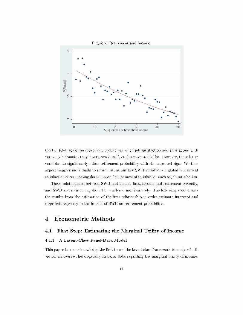
Figure 2: Retirement and Income

the EURO-D scale) on retirement probability when job satisfaction and satisfaction with

various job domains (pay, hours, work itself, etc.) are controlled for. However, these latter

variables do signi�cantly a�ect retirement probability with the expected sign. We thus

expect happier individuals to retire less, as our key SWB variable is a global measure of

satisfaction encompassing domain-speci�c measures of satisfaction such as job satisfaction.

These relationships between SWB and income �rst, income and retirement secondly,

and SWB and retirement, should be analysed multivariately. The following section uses

the results from the estimation of the �rst relationship in order estimate intercept and

slope heterogeneity in the impact of SWB on retirement probability.

4 Econometric Methods

4.1 First Step: Estimating the Marginal Utility of Income

4.1.1 A Latent-Class Panel-Data Model

This paper is to our knowledge the �rst to use the latent class framework to analyse indi-

vidual unobserved heterogeneity in panel data regarding the marginal utility of income.

11

The advantage of panel data in the identi�cation of latent class models was underlined

by Greene [2001].

We model individual heterogeneity in a �exible way, making no distributional assump-

tions for the unobserved individual e�ects. The FMM distinguishes between a �nite, usu-

ally small, number of latent classes of individuals (this number is C in the presentation

below), which can di�er in both the level of well-being and the relationship to the re-

gression covariates. Here we speci�cally concentrate on income. Conventional panel data

models (with �xed or random e�ects) only consider intercept heterogeneity.

The basic econometric model used to model SWB is:

E(WBt|INCt, Xt) = αINCt + βXt (1)

where our key explanatory variable is INC, the logarithm of total household income, and

Xt is a vector of individual characteristics (sociodemographic, labour market, economic,

regional and time variables). Equation 1 is �rst estimated by OLS, and here α/100 is the

absolute change in WB resulting from a 1% increase in income. However, if WB is drawn

from distinct subpopulations, the OLS estimate of α is the average of the e�ects across

subpopulations and may hide considerable heterogeneity. We therefore estimate a �nite

mixture model, where subpopulations are assumed to be drawn from normal distributions.

In the FMM the randomWB variable is considered as a draw from a population which

is an additive mixture of C distinct classes in proportions πj such that:

g(wbi | xi; θ1, ..., θC ;πi1, ..., πiC) =

C∑j=1

πij

Ti∏t=1

fj(wbit | xit, θj), (2)

0 ≤ πij ≤ 1,∑C

j=1 πij = 1, ∀i = 1, ..., N ;

where θj is the associated set of parameters, Ti = 1, ..., 8 is the number of times the

individual i is observed, and the density of component j for observation i is given by:

fj(wbit | xit, θj) =1

σj√

2πexp

(− 1

2σ2j

(wbit − αjINCit − βjXit)2

)(3)

The �nite mixture model is estimated using maximum likelihood and cluster-corrected (for

within-individual correlation) robust standard errors. Starting from the initial estimates

of component proportions πj , we then re-estimate the model assuming a prior component

12

probability of the form:

πij(Zi | δ) = Z ′iδ, 0 ≤ πij ≤ 1,

C∑j=1

πij = 1,∀i = 1, ..., N. (4)

The prior component probability πj now depends on observables Z and so varies across

observations. Individuals with di�erent observable characteristics then likely have di�er-

ent probabilities of belonging to the di�erent classes.

As put forward in Deb, Gallo, Ayyagari, Fletcher, and Sindelar [2009], �nite mixture

models have many advantages, but also some drawbacks. A �nite mixture model may

�t the data better than a basic OLS model due to outliers, which are captured in the

FMM via additional mixture components. Even if the use of FMM is motivated by ex

ante reasoning, the di�erent latent classes need to be justi�ed ex post.

The FMM model yields the prior and posterior probabilities of being in each of the

latent classes, conditional on all observed covariates (and also on the observed WB out-

come for the posterior probability). Using Bayes' theorem, the posterior probability of

being in component k is:

Pr(i ∈ k | θ, wbi) =πik∏Ti

t=1 fk(wbit | xit, θk)∑Cj=1 πij

∏Ti

t=1 fj(wbit | xit, θj), ∀k = 1, 2, ..., C. (5)

The posterior probability varies across observations, as does the prior probability when

re-estimated conditional on Z. The di�erence between these two is that posterior prob-

abilities are also conditional on the outcome wbi. The latter can of course be used to

explore the determinants of class membership, but in what follows we stick to the prior

probabilities for reasons that we will set out in Section 5.

4.1.2 Between Vs. Within

We use the panel nature of the data to distinguish the between-individual and within-

individual e�ects of our right-hand side variables. With respect to income, we can see

whether the marginal utility of income di�ers between individuals, but remains fairly

constant within-person over time. Deb and Trivedi [2011] provide a simpli�ed computa-

tion method to estimate a mixture of normal distributions with �xed e�ects. Replacing

(wbit, xit) by (w̃bit, x̃it), where˜denotes the �within transformation�, i.e. x̃i = xit − x̄,and then maximizing the mixture likelihood, is numerically equivalent to applying the

full EM algorithm for the estimation of a latent-class model with �xed e�ects. This kind

13

of estimation can then proceed in the same way as the standard FMM in cross-section

data. We use the same method to estimate �between� e�ects too, replacing (wbit, xit) by

the �between transformation� (w̄bi, x̄i), where x̄i =∑Ti

t=1 xit/Ti, and then estimating a

standard �nite mixture model on these transformed variables.

4.2 Second Step: Using the FMM Results to Predict Retirement

Latent-class analysis provides di�erent estimates of the marginal utility of income for

each group, the αk, ∀k = 1, 2, ..., C, along with the prior probabilities πk(Zi | δ) and

posterior probabilities Pr(i ∈ k | θ, wbi) of belonging to class k. We exploit this individual

heterogeneity to create a continuous measure of the marginal utility of income, de�ned

as:

e =

C∑k=1

αkπk(Zi | δ) (6)

We will then look for an impact of e on retirement probability by wave t+1 for individuals

who are in work at wave t. Our probit retirement-probability model is:

Pr(Retirei,t+1 = 1 | Vi,t) = Φ(V ′i,tγt) (7)

where Pr denotes the probability, φ is the cumulative distribution function of the standard

normal distribution, and V is a vector of covariates. The parameters γ are estimated by

maximum likelihood. Retirei,t+1 is a dummy coded 1 if individual i stops working between

waves t and t+ 1 and declares themselves to be �fully retired� at wave t+ 1, which is the

case for 15 per cent of our pooled sample.

5 Results

5.1 Results From Finite Mixture Models

5.1.1 Results from Pooled Estimations

We estimate the marginal utility of income using a simple OLS regression and a number

of speci�cations of a �nite mixture model. The model selection criteria (AIC/BIC) clearly

support a 2-component mixture model as compared to the 1-component OLS model. The

3-component model fails to converge after a reasonable number of iterations, suggesting

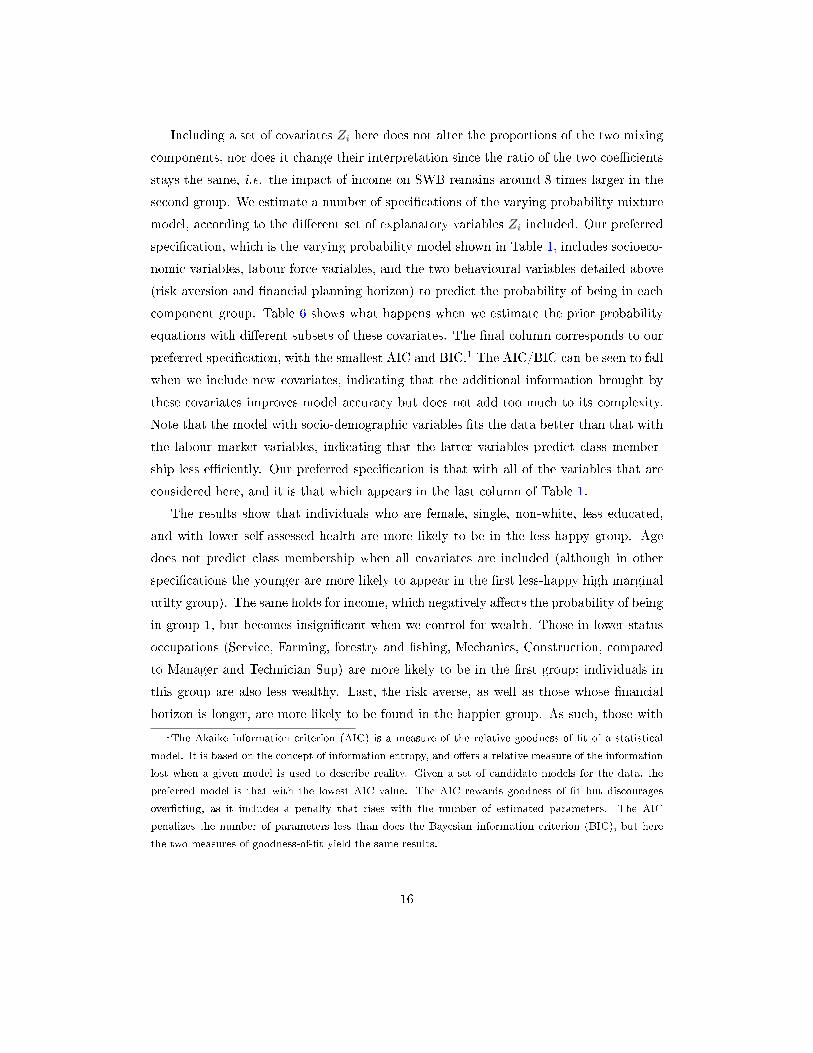
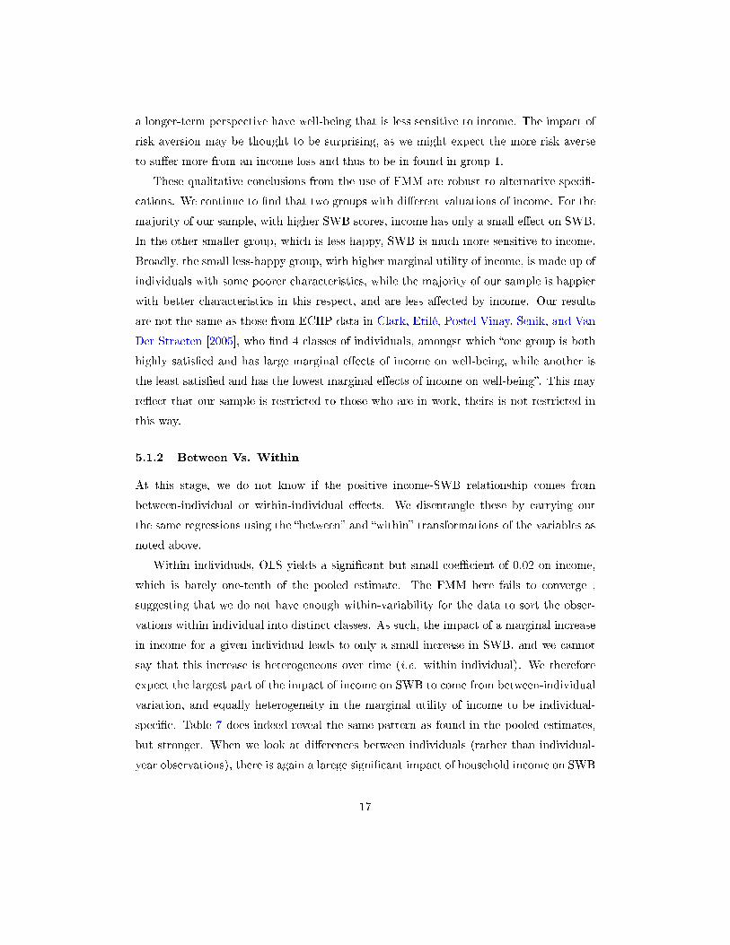
that the third component is trying to �t a small number of outliers. Table 1 shows

14

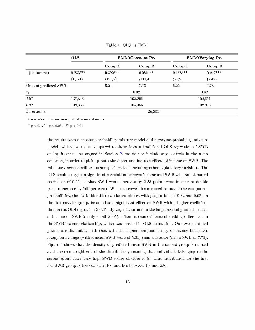
Table 1: OLS vs FMM

OLS FMM:Constant Pr. FMM:Varying Pr.

Comp.1 Comp.2 Comp.1 Comp.2

ln(hh income) 0.235*** 0.390*** 0.050*** 0.188*** 0.027***

(18.21) (12.57) (11.04) (7.39) (7.45)

Mean of predicted SWB 5.21 7.75 5.23 7.76

π1 0.32 0.32

AIC 138,348 105,296 102,611

BIC 138,365 105,356 102,976

Observations 36,283

t statistics in parentheses; robust standard errors

* p < 0.1, ** p < 0.05, *** p < 0.01

the results from a constant-probability mixture model and a varying-probability mixture

model, which are to be compared to those from a traditional OLS regression of SWB

on log income. As argued in Section 2, we do not include any controls in the main

equation, in order to pick up both the direct and indirect e�ects of income on SWB. The

robustness section will test other speci�cations including other explanatory variables. The

OLS results suggest a signi�cant correlation between income and SWB with an estimated

coe�cient of 0.23, so that SWB would increase by 0.23 points were income to double

(i.e. to increase by 100 per cent). When no covariates are used to model the component

probabilities, the FMM identi�es two latent classes with proportions of 0.32 and 0.68. In

the �rst smaller group, income has a signi�cant e�ect on SWB with a higher coe�cient

than in the OLS regression (0.39). By way of contrast, in the larger second group the e�ect

of income on SWB is only small (0.05). There is thus evidence of striking di�erences in

the SWB-income relationship, which was masked in OLS estimation. Our two identi�ed

groups are dissimilar, with that with the higher marginal utility of income being less

happy on average (with a mean SWB score of 5.21) than the other (mean SWB of 7.75).

Figure 4 shows that the density of predicted mean SWB in the second group is massed

at the extreme right end of the distribution, meaning that individuals belonging to the

second group have very high SWB scores of close to 8. This distribution for the �rst

low-SWB group is less concentrated and lies between 4.8 and 5.8.

15

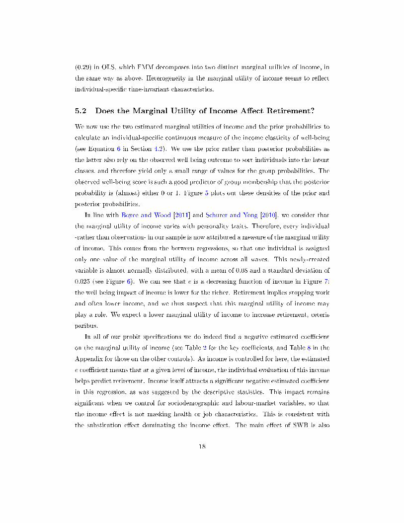
Including a set of covariates Zi here does not alter the proportions of the two mixing

components, nor does it change their interpretation since the ratio of the two coe�cients

stays the same, i.e. the impact of income on SWB remains around 8 times larger in the

second group. We estimate a number of speci�cations of the varying probability mixture

model, according to the di�erent set of explanatory variables Zi included. Our preferred

speci�cation, which is the varying probability model shown in Table 1, includes socioeco-

nomic variables, labour-force variables, and the two behavioural variables detailed above

(risk aversion and �nancial planning horizon) to predict the probability of being in each

component group. Table 6 shows what happens when we estimate the prior probability

equations with di�erent subsets of these covariates. The �nal column corresponds to our

preferred speci�cation, with the smallest AIC and BIC.1 The AIC/BIC can be seen to fall

when we include new covariates, indicating that the additional information brought by

these covariates improves model accuracy but does not add too much to its complexity.

Note that the model with socio-demographic variables �ts the data better than that with

the labour market variables, indicating that the latter variables predict class member-

ship less e�ciently. Our preferred speci�cation is that with all of the variables that are

considered here, and it is that which appears in the last column of Table 1.

The results show that individuals who are female, single, non-white, less educated,

and with lower self-assessed health are more likely to be in the less-happy group. Age

does not predict class membership when all covariates are included (although in other

speci�cations the younger are more likely to appear in the �rst less-happy high marginal

utilty group). The same holds for income, which negatively a�ects the probability of being

in group 1, but becomes insigni�cant when we control for wealth. Those in lower-status

occupations (Service, Farming, forestry and �shing, Mechanics, Construction, compared

to Manager and Technician Sup) are more likely to be in the �rst group; individuals in

this group are also less wealthy. Last, the risk averse, as well as those whose �nancial

horizon is longer, are more likely to be found in the happier group. As such, those with

1The Akaike information criterion (AIC) is a measure of the relative goodness of �t of a statistical

model. It is based on the concept of information entropy, and o�ers a relative measure of the information

lost when a given model is used to describe reality. Given a set of candidate models for the data, the

preferred model is that with the lowest AIC value. The AIC rewards goodness of �t but discourages

over�tting, as it includes a penalty that rises with the number of estimated parameters. The AIC

penalizes the number of parameters less than does the Bayesian information criterion (BIC), but here

the two measures of goodness-of-�t yield the same results.

16

a longer-term perspective have well-being that is less sensitive to income. The impact of

risk aversion may be thought to be surprising, as we might expect the more risk averse

to su�er more from an income loss and thus to be in found in group 1.

These qualitative conclusions from the use of FMM are robust to alternative speci�-

cations. We continue to �nd that two groups with di�erent valuations of income. For the

majority of our sample, with higher SWB scores, income has only a small e�ect on SWB.

In the other smaller group, which is less happy, SWB is much more sensitive to income.

Broadly, the small less-happy group, with higher marginal utility of income, is made up of

individuals with some poorer characteristics, while the majority of our sample is happier

with better characteristics in this respect, and are less a�ected by income. Our results

are not the same as those from ECHP data in Clark, Etilé, Postel-Vinay, Senik, and Van

Der Straeten [2005], who �nd 4 classes of individuals, amongst which �one group is both

highly satis�ed and has large marginal e�ects of income on well-being, while another is

the least satis�ed and has the lowest marginal e�ects of income on well-being�. This may

re�ect that our sample is restricted to those who are in work, theirs is not restricted in

this way.

5.1.2 Between Vs. Within

At this stage, we do not know if the positive income-SWB relationship comes from

between-individual or within-individual e�ects. We disentangle these by carrying out

the same regressions using the �between� and �within� transformations of the variables as

noted above.

Within individuals, OLS yields a signi�cant but small coe�cient of 0.02 on income,

which is barely one-tenth of the pooled estimate. The FMM here fails to converge ,

suggesting that we do not have enough within-variability for the data to sort the obser-

vations within individual into distinct classes. As such, the impact of a marginal increase

in income for a given individual leads to only a small increase in SWB, and we cannot

say that this increase is heterogeneous over time (i.e. within individual). We therefore

expect the largest part of the impact of income on SWB to come from between-individual

variation, and equally heterogeneity in the marginal utility of income to be individual-

speci�c. Table 7 does indeed reveal the same pattern as found in the pooled estimates,

but stronger. When we look at di�erences between individuals (rather than individual-

year observations), there is again a larege signi�cant impact of household income on SWB

17

(0.29) in OLS, which FMM decomposes into two distinct marginal utilities of income, in

the same way as above. Heterogeneity in the marginal utility of income seems to re�ect

individual-speci�c time-invariant characteristics.

5.2 Does the Marginal Utility of Income A�ect Retirement?

We now use the two estimated marginal utilities of income and the prior probabilities to

calculate an individual-speci�c continuous measure of the income elasticity of well-being

(see Equation 6 in Section 4.2). We use the prior rather than posterior probabilities as

the latter also rely on the observed well-being outcome to sort individuals into the latent

classes, and therefore yield only a small range of values for the group probabilities. The

observed well-being score is such a good predictor of group membership that the posterior

probability is (almost) either 0 or 1. Figure 5 plots out these densities of the prior and

posterior probabilities.

In line with Boyce and Wood [2011] and Schurer and Yong [2010], we consider that

the marginal utility of income varies with personality traits. Therefore, every individual

-rather than observation- in our sample is now attributed a measure of the marginal utility

of income. This comes from the between regressions, so that one individual is assigned

only one value of the marginal utility of income across all waves. This newly-created

variable is almost normally distributed, with a mean of 0.08 and a standard deviation of

0.025 (see Figure 6). We can see that e is a decreasing function of income in Figure 7:

the well-being impact of income is lower for the richer. Retirement implies stopping work

and often lower income, and we thus suspect that this marginal utility of income may

play a role. We expect a lower marginal utility of income to increase retirement, ceteris

paribus.

In all of our probit speci�cations we do indeed �nd a negative estimated coe�cient

on the marginal utility of income (see Table 2 for the key coe�cients, and Table 8 in the

Appendix for those on the other controls). As income is controlled for here, the estimated

e coe�cient means that at a given level of income, the individual evaluation of this income

helps predict retirement. Income itself attracts a signi�cant negative estimated coe�cient

in this regression, as was suggested by the descriptive statistics. This impact remains

signi�cant when we control for sociodemographic and labour-market variables, so that

the income e�ect is not masking health or job characteristics. This is consistent with

the substitution e�ect dominating the income e�ect. The main e�ect of SWB is also

18

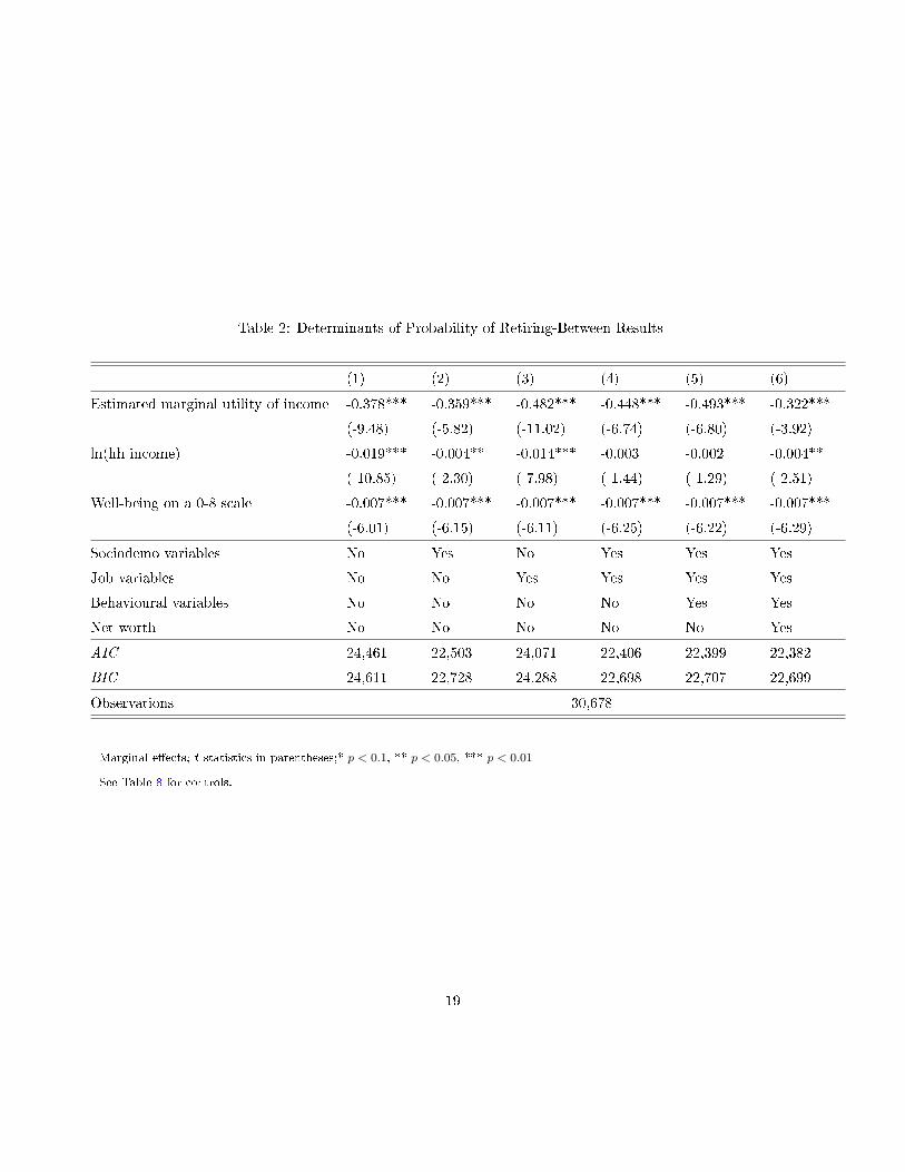
Table 2: Determinants of Probability of Retiring-Between Results

(1) (2) (3) (4) (5) (6)

Estimated marginal utility of income -0.378*** -0.359*** -0.482*** -0.448*** -0.493*** -0.322***

(-9.48) (-5.82) (-11.02) (-6.74) (-6.80) (-3.92)

ln(hh income) -0.019*** -0.004** -0.014*** -0.003 -0.002 -0.004**

(-10.85) (-2.30) (-7.98) (-1.44) (-1.29) (-2.51)

Well-being on a 0-8 scale -0.007*** -0.007*** -0.007*** -0.007*** -0.007*** -0.007***

(-6.01) (-6.15) (-6.11) (-6.25) (-6.22) (-6.29)

Sociodemo variables No Yes No Yes Yes Yes

Job variables No No Yes Yes Yes Yes

Behavioural variables No No No No Yes Yes

Net worth No No No No No Yes

AIC 24,461 22,503 24,071 22,406 22,399 22,382

BIC 24,611 22,728 24,288 22,698 22,707 22,699

Observations 30,678

Marginal e�ects; t statistics in parentheses;* p < 0.1, ** p < 0.05, *** p < 0.01

See Table 8 for controls.

19

negative too, again con�rming the suggestion in the descriptive statistics that happier

individuals retire less. The estimated coe�cients on income and SWB are signi�cant

across all speci�cations. Adding the log of net worth (column (6) compared to column

(5)) renders the impact of the marginal utility of income weaker in terms of maagnitude

but does not alter its signi�cance. As those with more wealth retire more, and wealth

is a strong negative predictor of the marginal utility of income (the wealthier have a

lower marginal utility of income), this variable seems to capture some of the negative

e�ect of e on the probability of retiring. In terms of goodness of �t, the AIC/BIC falls

as we add new control variables, indicating that the model is not overparameterized.

Again, labour-market variables a�ect prediction less than do sociodemographic variables,

so that gender, age, health and education are better predictors of retirement than are

labour-market characteristics.

Regarding the other controls (see Table 8), we �nd reasonable results. For example,

women, the less-educated, the older and those in worse health retire more. Part-time

workers retire more, perhaps because they have already started their retirement transition

by reducing their work hours.

5.3 Robustness Checks

As explained in Section 2, we estimate the marginal utility of income by regressing SWB

on income, without any other covariates in order to capture both the direct and indirect

e�ects of income. We have also tested other speci�cations with control variables. Column

(1) of Table 9 presents analogous results to those from the FMM with no controls in Table

1. We start with the more exogenous variables: gender, race, age, education, wave and

region. The data again sort into two groups with di�erent valuations of income in the

same way as beforehand. When all the variables in the Zi set are included, income loses

its explanatory power (probably because it is well-predicted by these Zi)). We thus use

the second speci�cation (2) to create a new marginal utility of income and see whether

this a�ects retirement: Table 10 con�rms our previous results in this respect.

Finally, we re-estimate our �fth speci�cation, includes all controls except net worth,

for various subsamples (e.g. individuals in a couple, with low/high education attainment,

and men and women). For brevity, we only present the estimates of the key parameters

in Table 11. The marginal utility of income remains signi�cant and negative in almost all

subsamples. It has a larger e�ect when income is also signi�cant: for the high-education

20

male group and the less-educated female group. The marginal e�ect of SWB is remarkably

stable across speci�cations.

6 Conclusion

This paper �rst modeled heterogeneity in the valuations of income using latent-class

analysis on nationally-representative data on US workers close to retirement. We identify

two classes of individuals with distinct marginal utilities of income. Our main results

indicate that there is a great deal of heterogeneity across the two latent classes. A

smaller group is relatively unhappy, with high marginal utility of income, and is made of

individuals with some poorer characteristics, while the majority group is happier, with

some nicer characteristics, and are less a�ected by income. The panel nature of our

data suggests that heterogeneity in the marginal utility of income is mostly between

individuals, rather than within-individual.

We then use these latent-class results to investigate the impact of the marginal utility

of income on retirement. We thus add to the existing retirement literature by considering a

�slope� impact of well-being upon the probability of retiring. We �nd a negative signi�cant

e�ect of the marginal utility of income on retirement, even controlling for the main e�ects

of income and well-being. Those who value income more retire less, regardless of how

much income they have. As retirement often implies lower income, a higher marginal

utility of income yields greater subjective and therefore later retirement.

These �ndings are pertinent in the current context of pensions. That the majority of

workers close to retirement care relatively less about the income drop from retirement,

while a smaller group is much more sensitive to this loss, might help policy makers in

designing labour-supply policy (by targeting the latter group). We also contribute to

validating SWB scores, by showing that both the level and slope of self-reported SWB

predict future behaviour.

A more general implication is that slope heterogeneity is probably worth further in-

vestigation: individuals di�er in ways that are not captured by simple �xed e�ects. Here

this heterogeneity helped to predict labour supply. Future applied work could usefully

appeal to slope heterogeneity to model many other kinds of individual behaviour. Finite

mixture models are likely to become a useful complement to the standard toolbox that

economists use to predict a wide variety of behaviour.

21

References

Aitkin, M., and D. B. Rubin (1985): �Estimation and Hypothesis Testing in Finite

Mixture Models,� Journal of the Royal Statistical Society. Series B (Methodological),

47(1), pp. 67�75.

Ayyagari, P., P. Deb, J. Fletcher, W. T. Gallo, and J. L. Sindelar (2009): �Sin

Taxes: Do Heterogeneous Responses Undercut Their Value?,� NBER Working Papers

15124, National Bureau of Economic Research, Inc.

Bender, K. A. (2004): �The Well-Being of Retirees: Evidence Using Subjective Data,�

Working Papers, Center for Retirement Research at Boston College 2004-24, Center

for Retirement Research.

Bonsang, E., and T. J. Klein (2011): �Retirement and Subjective Well-Being,� IZA

Discussion Papers 5536, Institute for the Study of Labor (IZA).

Borsch-Supan, A., and H. Jurges (2007): �Early Retirement, Social Security and

Well-Being in Germany,� MEA discussion paper series 07134, Mannheim Research In-

stitute for the Economics of Aging (MEA), University of Mannheim.

Boyce, C. J., and A. M. Wood (2011): �Personality and the marginal utility of income:

Personality interacts with increases in household income to determine life satisfaction,�

Journal of Economic Behavior & Organization, 78(1), 183�191.

Charles, K. (2004): �Is Retirement Depressing? Labour Force Inactivity and Psycholog-

ical Well-Being in Later Life.,� in Research in Labour Economics 23, ed. by S. Polachek,

Amsterdam. Elsevier.

Clark, A., F. Etilé, F. Postel-Vinay, C. Senik, and K. Van Der Straeten

(2005): �Heterogeneity in Reported Well-Being: Evidence from Twelve European Coun-

tries,� Economic Journal, 115(502), 118�132.

Clark, A. E. (2001): �What really matters in a job? Hedonic measurement using quit

data,� Labour Economics, 8(2), 223�242.

(2003): �Unemployment as a Social Norm: Psychological Evidence from Panel

Data,� Journal of Labor Economics, 21(2), 289�322.

22

Clark, A. E., Y. Georgellis, and P. Sanfey (1998): �Job Satisfaction, Wage

Changes and Quits: Evidence From Germany,� Research in Labor Economics, 17.

Clark, A. E., and A. J. Oswald (2002): �Well-Being in Panels,� Mimeo(DELTA).

Deb, P., W. T. Gallo, P. Ayyagari, J. M. Fletcher, and J. L. Sindelar (2009):

�Job Loss: Eat, Drink and Try to be Merry?,� NBER Working Papers 15122, National

Bureau of Economic Research, Inc.

Deb, P., and P. Trivedi (2011): �Finite Mixture for Panels with Fixed E�ects,� Hunter

College Department of Economics Working Papers 432, Hunter College: Department

of Economics.

Deb, P., and P. K. Trivedi (1997): �Demand for Medical Care by the Elderly: A

Finite Mixture Approach,� Journal of Applied Econometrics, 12(3), 313�36.

Debrand, T., and N. Sirven (2009): �Les Facteurs explicatifs du départ à la Retraite

en Europe,� Retraite et Société, 57, 35�53.

Dempster, A. P., N. M. Laird, and D. B. Rubin (1977): �Maximum Likelihood

from Incomplete Data via the EM Algorithm,� Journal of the Royal Statistical Society.

Series B (Methodological), 39(1), pp. 1�38.

Dolan, P., D. Fujiwara, and R. Metcalfe (2011): �A Step towards Valuing Utility

the Marginal and Cardinal Way,� CEP Discussion Papers dp1062, Centre for Economic

Performance, LSE.

Eckstein, Z., and K. I. Wolpin (1999): �Why youths drop out of high school: the

impact of preferences, opportunities and abilities,� Econometrica, 67, 1295?339.

Elder, H. W., and P. M. Rudolph (1999): �Does Retirement Planning A�ect the

Level of Retirement Satisfaction?,� Financial Services Review, 8(2), 117�127.

Fawaz, Y. (2009): �Prendre sa Retraite le Plus Tôt Possible : du Rêve à la Réalité?,�

Retraite et Société, 57(1).

Ferrer-i Carbonell, A., and P. Frijters (2004): �How Important is Methodology

for the estimates of the determinants of Happiness?,� Economic Journal, 114(497),

641�659.

23

Freeman, R. B. (1978): �Job Satisfaction as an Economic Variable,� American Eco-

nomic Review, 68(2), 135�41.

Frijters, P. (2000): �Do individuals try to maximize general satisfaction?,� Journal of

Economic Psychology, 21(3), 281�304.

Georgellis, Y., J. Sessions, and N. Tsitsianis (2007): �Pecuniary and non-pecuniary

aspects of self-employment survival,� The Quarterly Review of Economics and Finance,

47(1), 94�112.

Greene, W. (2001): �Fixed and Random E�ects in Nonlinear Models,� Working Pa-

pers 01-01, New York University, Leonard N. Stern School of Business, Department of

Economics.

Guven, C., C. Senik, and H. Stichnoth (2012): �You can't be happier than your wife.

Happiness gaps and divorce,� Journal of Economic Behavior & Organization, 82(1), 110

� 130.

Iaffaldano, M. T., and P. M. Muchinsky (1985): �Job Satisfaction and Job Perfor-

mance:A Meta-Analysis,� Psychology Bulletin, 97, 251�73.

Kahneman, D., B. L. Fredrickson, C. A. Schreiber, and D. A. Redelmeier

(1993): �When More Pain Is Preferred to Less: Adding a Better End,� Psychological

Science, 4(6), 401�405.

Kahneman, D., P. P. Wakker, and R. Sarin (1997): �Back to Bentham? Explo-

rations of Experienced Utility,� The Quarterly Journal of Economics, 112(2), 375�405.

Kim, J. E., and P. Moen (June 2001): �Is Retirement Good or Bad for Subjective

Well-Being?,� Current Directions in Psychological Science, 10, 83�86(4).

Kristensen, N., and N. Westergaard-Nielsen (2006): �Job satisfaction and quits -

Which job characteristics matters most?,� Danish Economic Journal, 144, 230�248.

Lindeboom, M., F. Portrait, and G. van den Berg (2002): �An econometric analy-

sis of the mental-health e�ects of major events in the life of older individuals,� Working

Paper Series 2002:19, IFAU - Institute for Labour Market Policy Evaluation.

Ostroff, C. (1992): �The Relationship between Satisfaction, Attitudes and Perfor-

mance: An Organizational Level Analysis,� Journal of Applied Psychology, 77, 963�74.

24

Panis, C. (2004): Pension Design and Structure: New Lessons from Behavioral Fi-

nancechap. Annuities and Retirement Well-Being. Oxford University Press.

Radloff, L. (1977): �The CES-D scale: A Self-report Depression Scale for Research in

the General Population,� Applied Psychological Measurement, 1, 385�401.

Rogers, J., K. Clow, and T. Kash (1994): �Increasing Job Satisfaction of Service

Personnel,� Journal of Service Management, 8, 14�26.

Ryan, R., and E. Deci (2000): �Self-determination theory and the facilitation of intrinsic

motivation, social development, and well-being,� American Psychologist, 55, 68�78.

Schurer, S., and J. Yong (2010): �Personality, Well-being and Heterogeneous Valu-

ations of Income and Work,� Melbourne Institute Working Paper Series wp2010n14,

Melbourne Institute of Applied Economic and Social Research, The University of Mel-

bourne.

Seitsamo, J. (2007): �Retirement Transition and Well-Being, a 16-year longitudinal

study,� Ph.D. thesis, University of Helsinki.

Senik, C. (2004): �When information dominates comparison: Learning from Russian

subjective panel data,� Journal of Public Economics, 88(9-10), 2099�2123.

(2005): �Income distribution and well-being: what can we learn from subjective

data?,� Journal of Economic Surveys, 19(1), 43�63.

Shiv, B., and J. Huber (2000): �The Impact of Anticipating Satisfaction on Consumer

Choice,� Journal of Consumer Research: An Interdisciplinary Quarterly, 27(2), 202�16.

Shultz, K. S., K. R. Morton, and J. R. Weckerle (1998): �The In�uence of Push

and Pull Factors on Voluntary and Involuntary Early Retirees' Retirement Decision

and Adjustment,� Journal of Vocational Behavior, 53(1), 45 � 57.

Thacher, J., and E. . Morey (2003): �Using individual characteristics and attitudinal

data to identify and characterize groups that vary signi�cantly in their preferences for

monument preservation: a latent class model,� University of Colorado at Boulder.

Tinbergen, J. (1991): �On the Measurement of Welfare,� Journal of Econometrics,

50(7), 7�13.

25

Winkelmann, L., and R. Winkelmann (1998): �Why Are the Unemployed So Un-

happy? Evidence from Panel Data,� Economica, 65(257), 1�15.

Wottiez, I., and J. Theeuwes (1998): �Well-being and Labor Market Status,� in The

Distribution of Welfare and Household Production: International Perspectives, ed. by

Jenkins, Kapteyn, and van Praag. Cambridge University Press.

26

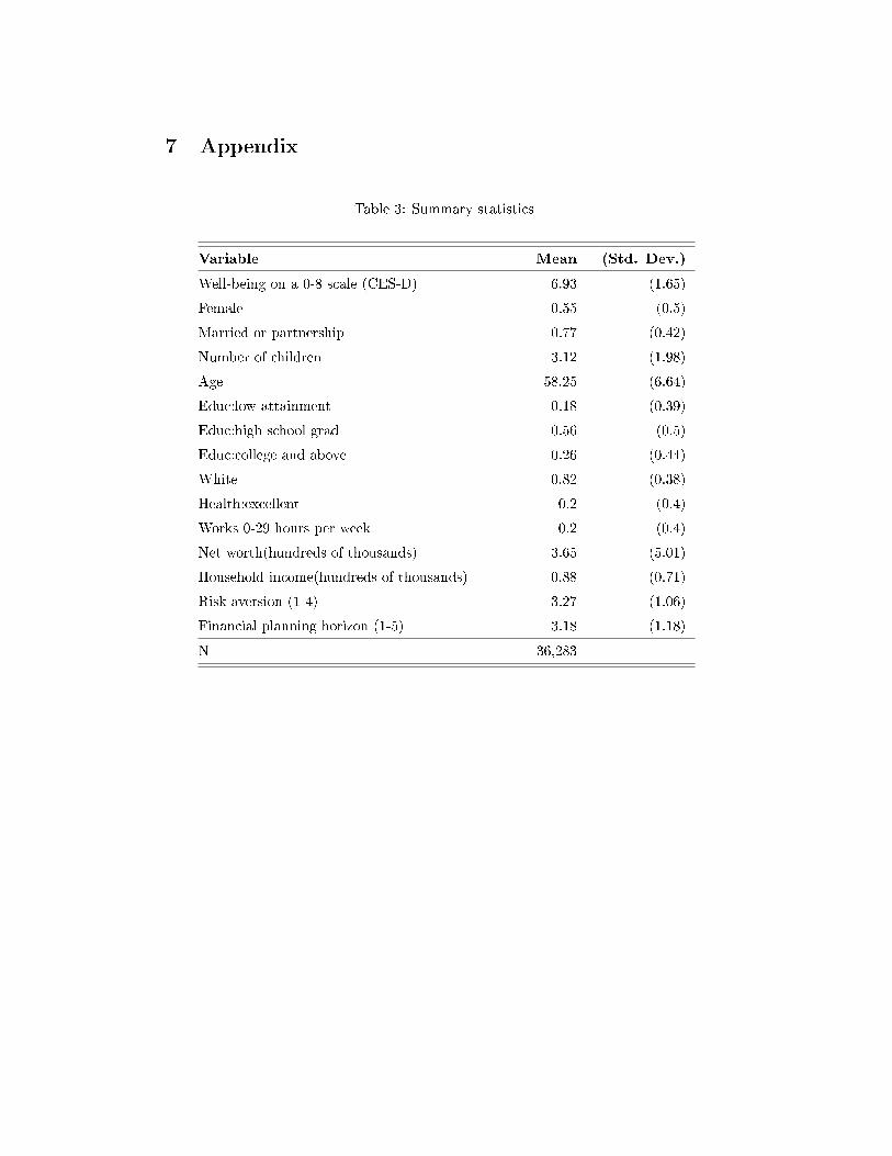
7 Appendix

Table 3: Summary statistics

Variable Mean (Std. Dev.)

Well-being on a 0-8 scale (CES-D) 6.93 (1.65)

Female 0.55 (0.5)

Married or partnership 0.77 (0.42)

Number of children 3.12 (1.98)

Age 58.25 (6.64)

Educ:low attainment 0.18 (0.39)

Educ:high school grad 0.56 (0.5)

Educ:college and above 0.26 (0.44)

White 0.82 (0.38)

Health:excellent 0.2 (0.4)

Works 0-29 hours per week 0.2 (0.4)

Net worth(hundreds of thousands) 3.65 (5.01)

Household income(hundreds of thousands) 0.88 (0.71)

Risk aversion (1-4) 3.27 (1.06)

Financial planning horizon (1-5) 3.18 (1.18)

N 36,283

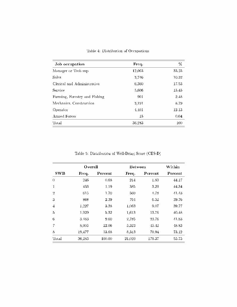
Table 4: Distribution of Occupations

Job occupation Freq. %

Manager or Tech sup 12,063 33.25

Sales 3,746 10.32

Clerical and Administrative 6,360 17.53

Service 5,606 15.45

Farming, Forestry and Fishing 901 2.48

Mechanics, Construction 3,191 8.79

Operator 4,401 12.13

Armed Forces 15 0.04

Total 36,283 100

Table 5: Distribution of Well-Being Score (CES-D)

Overall Between Within

SWB Freq. Percent Freq. Percent Percent

0 246 0.68 214 1.83 44.17

1 433 1.19 385 3.29 44.34

2 615 1.70 560 4.78 41.43

3 868 2.39 764 6.52 39.76

4 1,227 3.38 1,063 9.07 39.77

5 1,929 5.32 1,613 13.76 40.48

6 3,483 9.60 2,785 23.76 41.83

7 8,005 22.06 5,323 45.42 48.83

8 19,477 53.68 8,313 70.94 73.12

Total 36,283 100.00 21,020 179.37 55.75

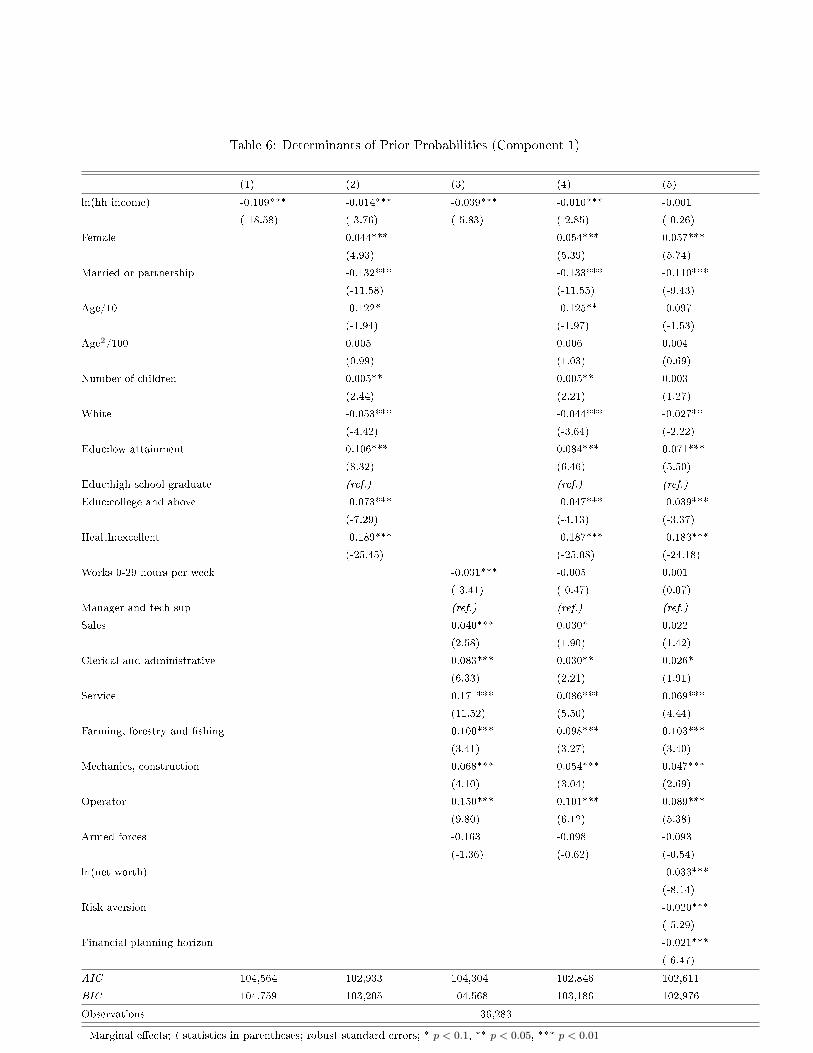
Table 6: Determinants of Prior Probabilities (Component 1)

(1) (2) (3) (4) (5)

ln(hh income) -0.109*** -0.014*** -0.039*** -0.010*** -0.001

(-18.58) (-3.76) (-5.83) (-2.85) (-0.26)

Female 0.044*** 0.054*** 0.057***

(4.93) (5.39) (5.74)

Married or partnership -0.132*** -0.133*** -0.110***

(-11.58) (-11.55) (-9.43)

Age/10 -0.122* -0.125** -0.097

(-1.94) (-1.97) (-1.53)

Age2/100 0.005 0.006 0.004

(0.99) (1.03) (0.69)

Number of children 0.005** 0.005** 0.003

(2.44) (2.21) (1.27)

White -0.053*** -0.044*** -0.027**

(-4.42) (-3.64) (-2.22)

Educ:low attainment 0.106*** 0.084*** 0.071***

(8.32) (6.46) (5.50)

Educ:high school graduate (ref.) (ref.) (ref.)

Educ:college and above -0.073*** -0.047*** -0.039***

(-7.29) (-4.13) (-3.37)

Health:excellent -0.189*** -0.187*** -0.183***

(-25.45) (-25.08) (-24.18)

Works 0-29 hours per week -0.031*** -0.005 0.001

(-3.41) (-0.47) (0.07)

Manager and tech sup (ref.) (ref.) (ref.)

Sales 0.040*** 0.030* 0.022

(2.58) (1.90) (1.42)

Clerical and administrative 0.083*** 0.030** 0.026*

(6.33) (2.21) (1.91)

Service 0.171*** 0.086*** 0.069***

(11.52) (5.50) (4.44)

Farming, forestry and �shing 0.100*** 0.098*** 0.103***

(3.41) (3.27) (3.40)

Mechanics, construction 0.068*** 0.054*** 0.047***

(4.10) (3.04) (2.69)

Operator 0.150*** 0.101*** 0.089***

(9.80) (6.12) (5.38)

Armed forces -0.163 -0.098 -0.093

(-1.36) (-0.62) (-0.54)

ln(net worth) -0.033***

(-8.14)

Risk aversion -0.020***

(-5.29)

Financial planning horizon -0.021***

(-6.47)

AIC 104,564 102,933 104,304 102,846 102,611

BIC 104,759 103,205 104,568 103,186 102,976

Observations 36,283

Marginal e�ects; t statistics in parentheses; robust standard errors; * p < 0.1, ** p < 0.05, *** p < 0.01

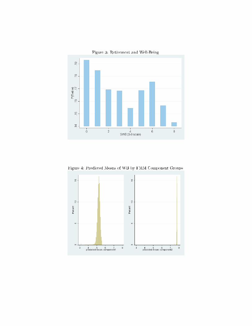
Figure 3: Retirement and Well-Being

Figure 4: Predicted Means of WB by FMM Component Groups

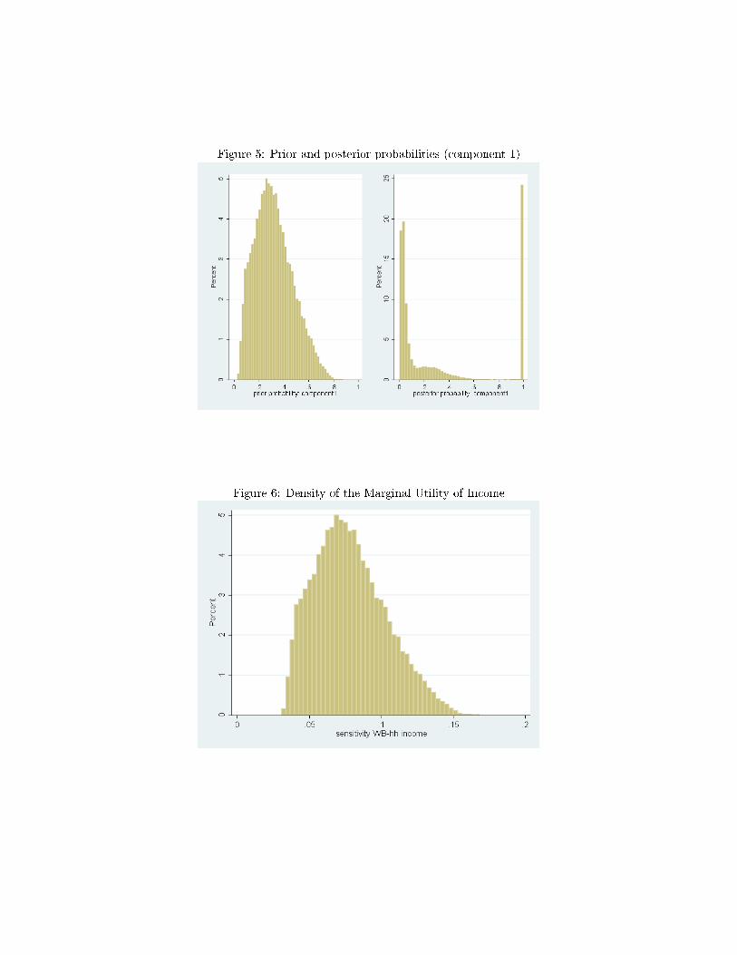
Figure 5: Prior and posterior probabilities (component 1)

Figure 6: Density of the Marginal Utility of Income

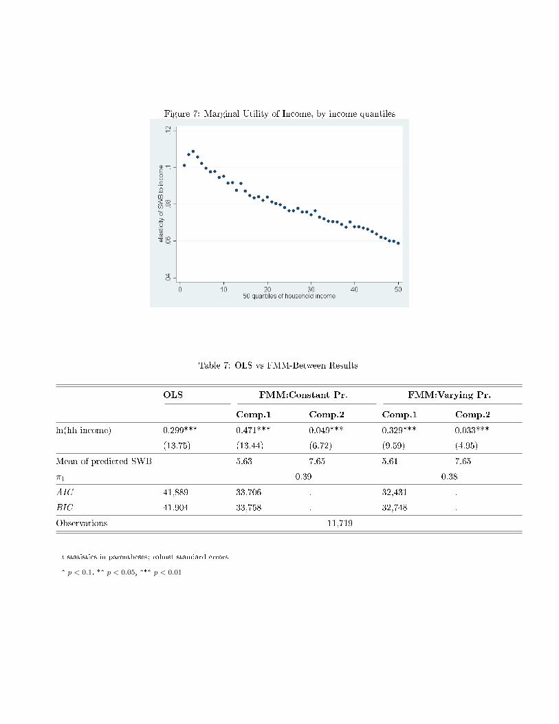
Figure 7: Marginal Utility of Income, by income quantiles

Table 7: OLS vs FMM-Between Results

OLS FMM:Constant Pr. FMM:Varying Pr.

Comp.1 Comp.2 Comp.1 Comp.2

ln(hh income) 0.299*** 0.471*** 0.049*** 0.329*** 0.033***

(13.75) (13.44) (6.72) (9.59) (4.95)

Mean of predicted SWB 5.63 7.65 5.61 7.65

π1 0.39 0.38

AIC 41,889 33,706 . 32,431 .

BIC 41,904 33,758 . 32,748 .

Observations 11,719

t statistics in parentheses; robust standard errors

* p < 0.1, ** p < 0.05, *** p < 0.01

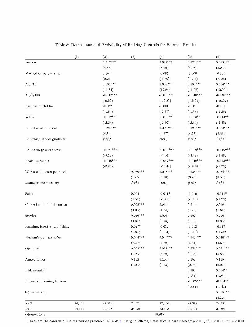
Table 8: Determinants of Probability of Retiring-Controls for Between Results

(1) (2) (3) (4) (5) (6)

Female 0.017*** 0.022*** 0.022*** 0.018***

(4.43) (5.00) (4.97) (3.93)

Married or partnership 0.001 -0.005 -0.006 -0.005

(0.27) (-0.89) (-1.14) (-0.86)

Age/10 0.692*** 0.698*** 0.693*** 0.694***

(11.84) (12.06) (11.95) (12.06)

Age2/100 -0.047*** -0.048*** -0.048*** -0.048***

(-9.92) (-10.27) (-10.21) (-10.27)

Number of children -0.002 -0.001 -0.001 -0.001

(-1.63) (-1.57) (-1.58) (-1.29)

White -0.012** -0.013** -0.013** -0.014**

(-2.23) (-2.40) (-2.39) (-2.45)

Educ:low attainment 0.026*** 0.025*** 0.026*** 0.023***

(4.31) (4.17) (4.23) (3.81)

Educ:high school graduate (ref.) (ref.) (ref.) (ref.)

Educ:college and above -0.024*** -0.019*** -0.019*** -0.019***

(-5.14) (-3.96) (-3.92) (-3.86)

Health:excellent -0.045*** -0.047*** -0.049*** -0.043***

(-9.84) (-10.44) (-10.48) (-8.75)

Works 0-29 hours per week 0.089*** 0.036*** 0.036*** 0.034***

(15.66) (6.86) (6.90) (6.58)

Manager and tech sup (ref.) (ref.) (ref.) (ref.)

Sales 0.004 -0.011* -0.010 -0.011*

(0.51) (-1.71) (-1.58) (-1.79)

Clerical and administrative 0.025*** 0.011* 0.011* 0.010

(4.00) (1.74) (1.75) (1.61)

Service 0.036*** 0.007 0.007 0.006

(4.81) (0.98) (1.05) (0.83)

Farming, forestry and �shing 0.027* -0.012 -0.012 -0.017

(1.87) (-1.04) (-1.06) (-1.58)

Mechanics, construction 0.064*** 0.041*** 0.042*** 0.040***

(7.49) (4.79) (4.84) (4.69)

Operator 0.068*** 0.034*** 0.036*** 0.031***

(8.23) (4.29) (4.37) (3.86)

Armed forces 0.112 0.109 0.109 0.119

(1.05) (0.93) (0.93) (0.97)

Risk aversion 0.002 0.004**

(1.34) (1.96)

Financial planning horizon -0.005*** -0.004**

(-2.81) (-2.43)

ln(net worth) 0.009***

(4.32)

AIC 24,461 22,503 24,071 22,406 22,399 22,382

BIC 24,611 22,728 24,288 22,698 22,707 22,699

Observations 30,678

These are the controls of the regressions presented in Table 2. Marginal e�ects; t statistics in parentheses;* p < 0.1, ** p < 0.05, *** p < 0.01

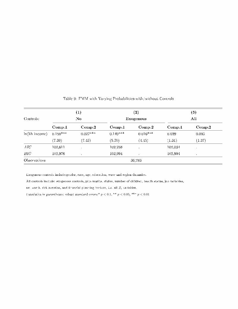
Table 9: FMM with Varying Probabilities-with/without Controls

(1) (2) (3)

Controls: No Exogenous All

Comp.1 Comp.2 Comp.1 Comp.2 Comp.1 Comp.2

ln(hh income) 0.188*** 0.027*** 0.149*** 0.016*** 0.039 0.005

(7.39) (7.45) (5.70) (4.45) (1.31) (1.37)

AIC 102,611 . 102,288 . 102,034 .

BIC 102,976 . 102,994 . 102,994 .

Observations 36,283

Exogenous controls include:gender, race, age, education, wave and region dummies.

All controls include: exogenous controls, plus marital status, number of children, health status, job variables,

net worth, risk aversion, and �nancial planning horizon, i.e. all Zi variables.

t statistics in parentheses; robust standard errors;* p < 0.1, ** p < 0.05, *** p < 0.01

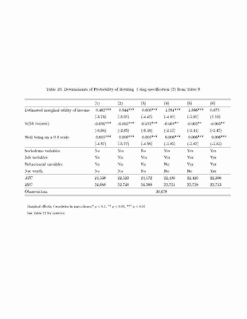
Table 10: Determinants of Probability of Retiring- Using speci�cation (2) from Table 9

(1) (2) (3) (4) (5) (6)

Estimated marginal utility of income -0.462*** -0.944*** -0.600*** -1.351*** -1.886*** 0.675

(-3.73) (-3.91) (-4.47) (-4.81) (-5.01) (1.10)

ln(hh income) -0.016*** -0.005*** -0.012*** -0.004** -0.005** -0.005**

(-8.98) (-2.65) (-6.48) (-2.17) (-2.44) (-2.47)

Well-being on a 0-8 scale -0.005*** -0.006*** -0.005*** -0.006*** -0.006*** -0.006***

(-4.37) (-5.77) (-4.38) (-5.85) (-5.87) (-5.85)

Sociodemo variables No Yes No Yes Yes Yes

Job variables No No Yes Yes Yes Yes

Behavioural variables No No No No Yes Yes

Net worth No No No No No Yes

AIC 24,538 22,523 24,172 22,430 22,420 22,396

BIC 24,688 22,748 24,388 22,721 22,728 22,713

Observations 30,678

Marginal e�ects; t statistics in parentheses;* p < 0.1, ** p < 0.05, *** p < 0.01

See Table ?? for controls

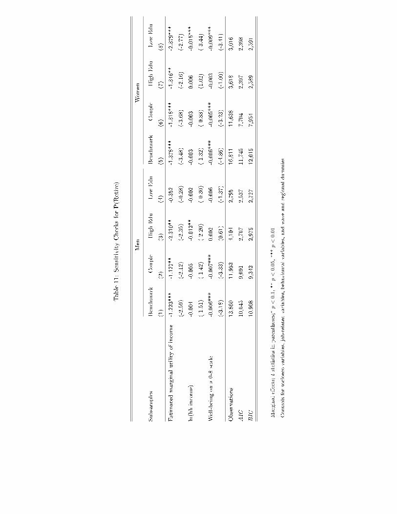
Table11:SensitivityChecksforP(R

etire)

Men

Women

Subsamples

Benchmark

Couple

HighEdu

Low

Edu

Benchmark

Couple

HighEdu

Low

Edu

(1)

(2)

(3)

(4)

(5)

(6)

(7)

(8)

Estim

atedmarginalutility

ofincome

-1.223***

-1.127**

-2.310**

-0.352

-1.378***

-1.818***

-1.846**

-2.879***

(-2.59)

(-2.12)

(-2.35)

(-0.28)

(-3.48)

(-3.68)

(-2.16)

(-2.77)

ln(hhincome)

-0.004

-0.005

-0.012**

-0.002

-0.003

-0.003

0.006

-0.015***

(-1.51)

(-1.42)

(-2.20)

(-0.30)

(-1.32)

(-0.88)

(1.02)

(-3.44)

Well-beingona0-8

scale

-0.006***

-0.007***

0.002

-0.006

-0.006***

-0.005***

-0.003

-0.009***

(-3.18)

(-3.33)

(0.61)

(-1.37)

(-4.86)

(-3.23)

(-1.00)

(-3.41)

Observations

13,860

11,952

4,104

2,795

16,811

11,638

3,618

3,016

AIC

10,645

9,091

2,767

2,537

11,745

7,704

2,397

2,398

BIC

10,908

9,342

2,975

2,727

12,015

7,954

2,589

2,591

Marginale�ects;tstatisticsin

parentheses;*

p<

0.1,**p<

0.05,***p<

0.01

Controlsforsocioecovariables,job-relatedvariables,behaviouralvariables,andwaveandregionaldummies