Embed Size (px)
Citation preview
Return on Investment on AI : The Case of Capital Requirement
Henri Fraisse1 & Matthias Laporte2
March 2021, WP #809
ABSTRACT
Taking advantage of granular data we measure the change in bank capital requirement resulting from the implementation of AI techniques to predict corporate defaults. For each of the largest banks operating in France we design an algorithm to build pseudo-internal models of credit risk management for a range of methodologies extensively used in AI (random forest, gradient boosting, ridge regression, deep learning). We compare these models to the traditional model usually in place that basically relies on a combination of logistic regression and expert judgement. The comparison is made along two sets of criterias capturing : the ability to pass compliance tests used by the regulators during on-site missions of model validation (i), and the induced changes in capital requirement (ii). The different models show noticeable differences in their ability to pass the regulatory tests and to lead to a reduction in capital requirement. While displaying a similar ability than the traditional model to pass compliance tests, neural networks provide the strongest incentive for banks to apply AI models for their internal model of credit risk of corporate businesses as they lead in some cases to sizeable reduction in capital requirement.3
Keywords: Artificial Intelligence, Credit Risk, Regulatory Requirement.
JEL classification: C4, C55, G21, K35
1 Banque de France, [email protected] 2 Banque de France, [email protected] 3 Acknowledgments and disclaimer: We are very grateful to Wassim Le Lann for detailed comments and discussion of a previous version of the paper. We also thank participants to Banque de France internal seminar and participants to the 2020 conference on advanced econometrics applied to finance of the University of Paris, Nanterre. The views expressed in this paper are the authors’ and should not be read or quoted as representing those of
Banque de France or the ECB.
Banque de France WP #809 ii
NON-TECHNICAL SUMMARY
Over the recent years, the opportunity offered by Artifical Intelligence (“AI” hereafter) for optimizing processes in the financial services industry has been subject to considerable attention. Banks have been using statistical models for managing their risk for years. Following the Basel II accords signed in 2004, they have the possibility to use these internal models to estimate their own funds requirements – i.e. the minimum amount of capital they must hold by law – provided they have prior authorisation from their supervisor (the “advanced approach”). In France, banks elaborated their internal models in the years preceeding their actual validation –mostly in 2008- at a time when traditional techniques were prevailing and AI techniques could not been implemented or were not considered. In this paper, taking advantage of granular data we measure to which extent banks can lower their capital requirement by the use of AI techniques under the constraint to get their internal models approved by the supervisor. We set up a traditional model for each of the major banking groups operating in France in the corporate loans market. This traditional model – based on on a combination of logistic regression and expert judgemen– aims to replicate the models described in the regulatory validation reports and put in place by banks for predicting corporate defaults and computing capital requirement. On the same data, we then estimate pseudo “internal” models of corporate defauts using the four most extensively used in the AI field : neural networks, random forest, gradient boosting and penalized ridge regression.
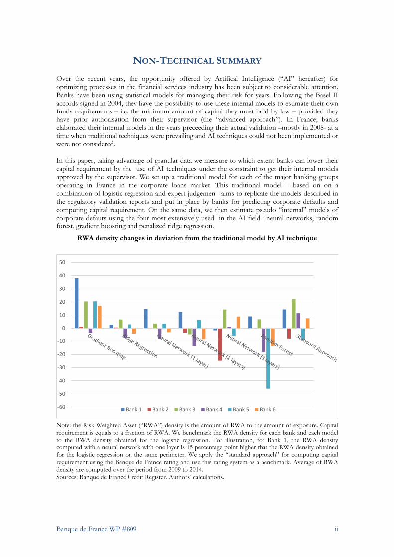
RWA density changes in deviation from the traditional model by AI technique
Note: the Risk Weighted Asset (“RWA”) density is the amount of RWA to the amount of exposure. Capital requirement is equals to a fraction of RWA. We benchmark the RWA density for each bank and each model to the RWA density obtained for the logistic regression. For illustration, for Bank 1, the RWA density computed with a neural network with one layer is 15 percentage point higher that the RWA density obtained for the logistic regression on the same perimeter. We apply the “standard approach” for computing capital requirement using the Banque de France rating and use this rating system as a benchmark. Average of RWA density are computed over the period from 2009 to 2014. Sources: Banque de France Credit Register. Authors’ calculations.
-60
-50
-40
-30
-20
-10
0
10
20
30
40
50
Bank 1 Bank 2 Bank 3 Bank 4 Bank 5 Bank 6
Banque de France WP #809 iii
We compare these models to the traditional model along two sets of criterias capturing : the ability to pass compliance tests used by the regulators during on-site missions of model validation (i), and the induced changes in capital requirement (ii). The different models show noticeable differences in their ability to pass the regulatory tests and to lead to a reduction in capital requirement. Prone to overfitting, the random forest methodology fails the compliance tests. The gradient boosting methodology leads to capital charge higher than the one expected by regulators when no model is in place. While displaying a similar ability than the traditional model to pass compliance tests, neural networks provide in some cases strong incentive for banks to apply AI models for their internal model of credit risk of corporate businesses as they lead to sizeable reduction in capital requirement.
Une mesure du gain à utiliser l’IA : le cas des exigences en fonds propres bancaires
RÉSUMÉ Tirant parti des données granulaires, nous mesurons l'évolution des exigences de capital bancaire résultant de la mise en œuvre de techniques d'Intelligence Artificielle (« IA ») pour prédire les défauts de l'entreprise. Pour chacune des plus grandes banques opérant en France, nous construisons un algorithme pour élaborer des pseudo modèles internes de gestion du risque de crédit pour une gamme de méthodologies largement utilisées en IA (forêt aléatoire, boosting de gradient, régression de crête, deep learning). Nous comparons ces modèles au modèle traditionnel généralement en place qui repose essentiellement sur une combinaison de régression logistique et de jugement d'expert. La comparaison se fait selon deux critères: la capacité à passer les tests de conformité utilisés par les régulateurs lors des missions sur site de validation du modèle (i) et les évolutions induites du capital requis (ii). Les différents modèles montrent des différences notables dans leur capacité à passer les tests réglementaires et à conduire à une réduction des exigences de fonds propres. Tout en affichant une capacité similaire à celle du modèle traditionnel pour réussir les tests de conformité, les réseaux de neurones offrent la plus forte incitation pour les banques à appliquer des modèles d'IA pour leur modèle interne de risque de crédit des entreprises, car ils conduisent dans certains cas à une réduction importante des exigences de capital. Mots-clés : intelligence artificielle, risque de crédit, capital bancaire réglementaire.
Les Documents de travail reflètent les idées personnelles de leurs auteurs et n'expriment pas nécessairement la position de la Banque de France. Ils sont disponibles sur publications.banque-france.fr

1
Over the recent years, the opportunity offered by Artifical Intelligence (“AI” hereafter) for
optimizing processes in the financial services industry has been subject to considerable media
hype and promotions from consultancy firms. AI techniques have indeed potential applications
in a vast variety of areas : lending decision, investment strategies, compliance (See Wall 2018).
Banks have been using statistical techniques for managing their risk for years. However, one
could distinguish “traditional techniques” – typically logistic regression for predicting defaults,
see Kandani et al. (2010) – with the ones the AI community recently brought up to date thanks
to cheaper computing ressources and more accessible data –typically neural networks.
Following the Basel II accords signed in 2004, banks have the possibility to use internal models
to estimate their own funds requirements – i.e. the minimum amount of capital they must hold
by law – provided they have prior authorisation from their supervisor (the “advanced
approach”). Without this authorization, banks estimate their own fund using risk weight relying
on external rating attributed to their counterparties (the “standardized approach”). In France,
banks elaborated their internal models in the years preceeding their actual validation –mostly
in 2008- at a time when traditional techniques were prevailing and AI techniques could not been
implemented or were not considered.
In this paper, taking advantage of granular data we measure to which extent banks can lower
their capital requirement by the use of AI techniques under the constraint to get their internal
models approved by the supervisor. For this purpose, based on confidential regulatory
validation reports, we set up a benchmark model for each of the major banking groups operating
in France in the corporate loans market. This benchmark model – based on logistic regressions
– aims to replicate the models put in place by banks for predicting corporate defaults and
computing capital requirement. On the same data, we then estimate pseudo “internal” models
of corporate defauts using the four most extensively used in the AI field : neural networks,
random forest, gradient boosting and penalized ridge regression.1
An internal model of risk management is made of three blocks. The first block consists
in estimating a continuous risk score expressed as a function of risk drivers. The second block
is a discrete risk scale expressed as a function of the continuous risk score : firms are grouped
into R rating grades accordingly to constraints in terms of risk score homogeneity within a grade
and risk score heterogeneity between grades. The third block is a set of probability of default
1 See for a brief description of this approach :

2
associated to each grade of the rating system. Typically, these probabilities are some long term
average of the default rate of the exposures belonging to the grade. They are the key inputs for
computing capital requirement.
For each of the statistical technique under review, we implement an algorithm in order to have
the highest likelihood for the internal model derived from this technique to meet the requirement
outlined by the supervisors. These requirements are the quantitative tests set out by the Targeted
Review of Internal Models guide which has been used by the on-site assessment teams of the
ECB over the 2017-2019 period for checking the consistency and the compliance of the internal
models in use in the European banks supervised by the ECB. We are then able to compare
models across banks and within a given bank in light of their ability to reduce the capital
charges under the constraint to meet regulatory expectations.
What we find.
Prone to overfitting, the random forest methodology fails the compliance tests. The gradient
boosting methodology leads to capital charge higher than the one expected by regulators when
no model is in place (the “standardized approach” in the Basel II framework). Neural networks
as well traditional logistic regressions both pass the compliance tests but the former provide
higher capital gains. The choice of a given statistical model both impacts the likelihood to get
the regulatory approval and the level of capital requirement.
Contribution to the litterature
We contribute to the literature by providing an empirical exercice using granular data set and
AI techniques for predicting corporate defaults. We answer the question whether AI techniques
improves the risk management of financial institutions by predicting more accurately corporate
defaults. We measure to which extent banks have incentives to invest in AI techniques at the
light of capital requirement economy induced by these techniques. We document the fact that
the level of capital requirement depends on the statistical methodology used by the bank for
setting up its internal models.
The related literature
First, our paper can be linked to the economic literature of banking. Two recent interesting
results from this literature are that capital requirement have a strong impact on credit
3
distribution and real corporate outcomes (see for instance Behn et al. 2016, Fraisse et al. 2020)
and that banks might be able to manipulate risk weights in order to minimize their capital
requirements (see Behn et al. (2016) in the German case and Plosser and Santos (2018) in the
US case). Our results show that –beyond the manipulation issue since we operate under the
constraint to pass conformity tests- different statistical technics might lead to substantial change
in capital requirement. Consequently, these diffrences might have strong impacts on the real
economy and financial stability.
Second, our paper can be related to the “applied statistics” literature measuring the value
added brought by AI techniques. As noted by Hurlin and Pérignon (2019), the academic
literature of the early 2000s show mixed results in support of the more advanced AI technique.
Thomas (2000) or Baesens et al. (2003) shows that the gain of AI technique in predicting default
is limited in comparison with the logistic regression. Despite the new buzz on AI over more
recent years, the academic literature on credit default forecasting using AI algorithms is still
limited and is mostly focused on the retail sector : Khandani et al. (2010) investigate the ability
of AI to predict the default of consumer loans across six banks operating in the US while
Albanesi and Vamossy (2019) assess the performance of IA techniques on the defaulting of
credit card accounts. Closer to our work Barboza et al. (2017) and Moscatelli et al. (2019) apply
AI techniques and compare their performances for predicting corporate defaults. We
complement their approach by considering additional AI techniques on a comprehensive data
set2. In addition to all these papers, relying on supervisory validation reports and inspection
guides we implement an algorithm in order to compute the corresponding capital requirement.
The remainder of the paper is organized as follows: Section I presents the methodology with
a particular emphasis on the algorithm for the construction of the internal models and the
computation of the capital requirement. Section II describes the data and provides descriptive
statistics. Section III discusses the main results and section IV presents some robustness checks.
Section V provides concluding remarks.
I. Methodology
This section describes how banks construct their internal models and compute their capital
requirement. An internal model consists basically in three main blocks :
2 Barboza et al. (2017) and Moscatelli et al. (2019) do not consider neural networks. Barboza et al. (2017) use a sample of North-
American firms. Moscatelli et al. (2019) use the Italian credit register.
4
(i) A continuous risk score expressed as a function of risk drivers : this risk score is
usually obtained through a logistic regression regressing a dummy variable -equaling
one if the firm default over a one year horizon- on a limited number of explanory
variables supposedly driving the firm financial health ;
(ii) A discrete risk scale expressed as a function of the continuous risk score : firms are
grouped into R rating grades accordingly to constraints in terms of risk score
homogeneity within a grade and risk score heterogeneity between grades
(iii) A probability of default 𝑃𝐷 is associated to each grade. Typically, 𝑃𝐷 is some
long term average of the default rate of the exposures belonging to the grade (more
on this below).
The Basel formula allows to compute the capital requirement corresponding to the 𝑟(𝑗)
facility belonging to the rating class r as a function of the probability of default of this rating
class:3
𝐶𝑅 , ( ) = 𝑓 𝑃𝐷 , 𝐸𝑥𝑝𝑜𝑠𝑢𝑟𝑒 ( )
The total capital requirement is then obtained by summing 𝐶𝑅 , ( ) over the R rating grades.
that we normalize by the total of exposures :
𝐶𝑅 = 𝐶𝑅 , ( )
Where 𝐽 denotes the number of exposures of the grade r
Risk-weighted assets (“RWA” hereafter) are determined by multiplying CR by 12.5.4 In the
current European regulation, changes which result in a decrease of at least 5 % of the risk-
weighted exposure amounts for credit with the range of application of the internal rating system
are to be approved by the supervisor.5 An on-site supervisory investigation might be required
3More precisely the Basel formulas are :
𝐶𝑅 , = 𝐿𝐺𝐷. 𝑁 (1 − 𝑅) . 𝐺(𝑃𝐷 ) +𝑅
1 − 1
,
𝐺(𝑂. 99) − 𝑃𝐷 . 𝐿𝐺𝐷 ∗ (1 − 1.5. 𝑏) ∗ 1 + (𝑀 − 2.5) ∗ 𝑏) ∗ 1.06 ∗ 𝐸𝑥𝑝𝑜𝑠𝑢𝑟𝑒
Where :
𝑅 = 0.12 ∗1 − 𝑒( ∗ )
1 − 𝑒( )+ 0.24 ∗ 1 −
1 − 𝑒( ∗ )
1 − 𝑒( )− 0.04 ∗ 1 −
𝑚𝑖𝑛(𝑚𝑎𝑥(5, 𝑆), 50) − 5
45
And 𝑏 = 0.11852 − 0.05487. 𝑙𝑛(𝑃𝐷)
CR denotes the risk-weight or capital requirement, R the correlation, b an adjustment factor, S the total annual sales in millions. PD the probability of default , LGD the loss given default, M the maturity. N(x) is the cdf of the normal distribution N(0,1) and G(z) is the reciprocal of this cdf. To compute capital requirement, we assume a 45% LGD. The 45% are the LGD that were used in the so-called Basel II foundation approach that the bank could use in absence of a validated LGD model but with a validated PD model.
4 1/12.5=0.085. 8,5% is the minimu solvency ratio. 5 See : Delegated Regulation (EU) No 529/2014 and https://www.bankingsupervision.europa.eu/banking/tasks/internal_models/imi/html/index.en.html for a description of the process.

5
for this approval. The outcome of this investigation might be to reject the application of the
bank for using this model to compute its RWA. We therefore use the RWA density (e.g. the
RWA divided by the total of exposure) for capturing the incentive the banks might have in
adopting a new model.
In this paper, the distinction between AI models and the benckmark model operates only
through the first block of the internal model. For the two following blocks : the building of the
rating scale of R grades and the computation of the 𝑃𝐷 , we implement an common alogrithm
common across banks and models. Starting from one risk score function estimated using a given
technique on a given bank’s portfolio, this algorithm aims at build the internal rating system
the most robust to pass the compliance tests set out by the regulators. We then associate to each
of the internal rating system the most conservative set of PD.
A. Risk score : the benchmark model
We review the supervisory validation reports describing the internal models put in place by
banks for assessing SME risks and computing capital requirement. Internal models were
validated for four of the six banks as soon as 2008. One was validated in 2011 and another one
was validated in 2014 with a capital add-on. In all cases, we observe a mixture of a quantitative
approach and a qualitative approach. The qualitative approach consists in a pre-selection of
key risk drivers following discussions with the business lines. It is followed by a quantitative
approach : the statistical significance of the risk drivers is tested using a logistic regression and
a parcimonial approach. It is worthnoting that most of the French banks models on the corporate
sector were validated before the boom of AI.6 Note also that those models were even developped
before the validation date : in the early 2000s in the anticipation of the Basel II accord which
was signed in 2004.
We replicate this approach for each bank of the sample using both the expertise of the Banque
de France in rating corporate businesses and the comprehensive data available at the Banque de
France. Our qualitative approach consists in selecting the risk drivers used by Banque de
France analysts and compiled by the rating methodology division of the Banque de France.
These risk drivers are taken from the FIBEN data set (see the section on the data set below).
6According to Stuart Russel, the current AI epoch started around 2010. See “The impact of machine learning and AI on the UK
economy” by David Bholat, VOX article, 2 july 2020.

6
Note that some of these risk drivers are provided to banks in parallel since banks could pay for
getting FIBEN data and the Banque de France corporate financial analysis. Some risk drivers
have also been selected since they were considere by the rating methodology unit of the Banque
de France when computing and improving the Banque de France quantitative score (see table 1
in appendix for the list of indicators put in different broad themes of the credit analysis :
structural caracteristics, financial autonomy, financial structure, profitability, profit sharing,
productivity, rentability). The quantitative approach of the benchmark model consists in the
selection of indicators among the list of these risk drivers following five steps :
1. We discard indicators with more than 20% of missing values
2. When two indicators are highly correlated (above 0.7), we keep the ones with fewer
missing values
3. We discretize each indicator into 5 quintiles and a class of missing value
4. For each discretized indicator, we run a logistic regression including industry, judicial
status and size fixed effects on the default indicator. We select the indicator for which
the highest AUC (standing for Area Under (ROC) Curve) is reached.7
5. We then add indicators sequentially in the logistic regression while the AUC is
increasing. We stop when each additional variable tested lead to the same AUC within
a 0.2% range.
B. Risk score : the AI models
Starting from all the available indicators, we implement the four most popular AI techniques
for binary classification: random forests, gradient boosting, neural networks and ridge
classifiers. By training those models to predict the occurrence of default in a one year horizon,
we will obtain a continuous score going from 0 to 1 and corresponding to the confidence of the
predictor that the given firm will default in a one year horizon.
77 The AUC is one of the most common indicator used to evaluate the discriminatory power of a credit risk model. The true
positive rate is the fraction of actual defaults out of the defaults predicted by the model for a given probability threshold s (e.g. if the predicted probability is above s the exposure is predicted as defaulting). The false positive rate is the fraction of actual performing exposures out of the exposures predicted as defaulting by the model for the same given probability threshold s. The ROC curve plots the true positive rate versus the true negative rate at all threshold s in [0,1]. The AUC is the area under the ROC curve. It is a number between 0,5 and 1. 0,5 corresponds to the AUC of a model predicting the default at random.
7
Each of the classifiers are fitted using standard techniques including cross-validation8 in order
to tune hyper-parameters to prevent overfitting.9 For that, we use the sklearn open source
package for Python. We proceed to a:
Grid search over the maximum depth of the trees for trees ensembles classifiers
(random forests and gradient boosting)10;
Grid search over the regularization parameter for models with penalized loss
function (neural networks and ridge classifier)11;
Multiple random initialization of the weights for classifiers that can be specifically
sensitive to it (gradient boosting and neural networks)12.
Prior to fitting the classifiers, we apply the following custom preprocessing stage on the raw
numeric indicators:
Pseudo log-normalization of all indicators applying the transformation;
𝑦 = sign(𝑥) ∗ log(1 + |𝑥[)
Missing values imputation applying a custom mono variate statistical regressor on
default rate described in annex 1;
Standard-scaling by centering to the average and reducing the standard deviation to
1.
The categorical indicators are simply “one-hot” encoded (simple dummyfication).
In the end of the training process, we have a scoring model computing a continuous risk score
from an input vector of explanatory variables (preprocessed indicators from list A), and
calibrated on historical defaults.
C. Computation of capital requirement
a. An algorithm to set up the rating scale
The 2019 ECB TRIM guide details the regulatory expectations regarding internal models in
the background of the European wide campaign launched during the year 2019. This campaign
8 6-fold cross-validation based on a one year (4 quarters) vs. all chronological split 9 See appendix 1 for a detailed description of the strategies implemented to calibrate the models. 10 This parameter controls the complexity of the models and allows thus to adjust their learning capacity to avoid over-fitting and
keep a good out of sample performance 11 This parameter smoothen the optimization surface and improves the convergence of the model as well as reducing over-fitting 12 This ensures a good convergence of the models during the learning phase (ie. optimization of the model’s loss function on the
training dataset).

8
aimed at guaranteeing the consistency of internal models across European banks under the IRB
approach. In the guide, internal models are chiefly assessed along two dimensions : their ability
to accurately predict defaults and their discriminatory power for differentiating low risk from
high risk exposures. 13 To this respect, they should lead to a rating system without excessive
concentration of exposure per grade. They should lead to a risk homonegenity of exposures
within each grade and a risk heterogeneity of exposures between grades. In addition, the rating
system should not display “risk inversion” over the years e.g. the default rate observed for a
better grade should not become higher than the default rate of the adjacent worse rating grade.
These requirements are translated into quantitative tests. The main indicator of discriminatory
power prescribed by the ECB inspection guide is the AUC. A strong decrease in the AUC
should not be observed over recent periods (A decrease of more than 5 ppt is a warning).14 Risk
heterogeneity of grades is assessed using Z-tests : for each year and for each grade of the rating
scale, a “Z-test” is performed comparing the proportion of defaults observed in the grade with
the proportion of defaults observed in the adjacent grades.
In order to fulfill these requirements, we implement the following algorithm : for each quarter
of the training sample, we create a quarter specific scale by performing a recursive dichotomy
based on a descending hierarchical segmentation. This recursive dichotomy is performed as
follows:
For a given quarter, we sort the firms by ascending risk score ;
starting from an initial scale consisting in a single risk class (scores from 0 to 1), we
look for an optimal threshold score splitting the scale in two segments with minimal
intra-class variance on each side ;
we compute the global proportion of default 𝑅 as well as the proportions of
defaults on each of the two contiguous risk classes we just obtained (respectively 𝑅
for the “left” class and 𝑅 for the “right” class) and their frequencies (respectively 𝑁
for the “left” class and 𝑁 for the “right” class) ;
we check if they pass the Z-test at a 10% p-value level15, that is
(𝑅 − 𝑅 )/ 𝑅 ∗ 1 − 𝑅 ∗1
𝑁+
1
𝑁> 1.64485
13 See the section on “risk differentiation” in the guide. 14 Note that the TRIM guides proposes a formal statistical test as well. 15 ie. the default rate on the “left” class is significantly lower than it is on the “right” class

9
if so, we recursively try so split again each of those two resulting classes
independently, each time by minimizing the intra-class variance between the two
new sub-classes ;
at each stage, we check if the risk differentiation Z-test passes on both side of each
sub-class16, if so we keep on applying the recursion, if not we discard the potential
split and stop trying to split the parent sub-class ;
at some point, the recursion stops as none of the sub-classes can be split anymore17
and the resulting sequence of risk sub-classes constitutes the grades of the quarter
specific risk scale.
If this rating scale is not perfectly robust meaning that some Z-test fail for some quarter and
some pairs of adjacent grades, we iteratively improve it by merging grades that induce poor
differentiation18 until it becomes fully robust19 or there are only 7 grades left. 20
For each quarter specific risk scale, we compute a robustness score equaling the share of Z-
tests successfully passed between adjacent grades averaged over the training period. We then
select the rating scale maximizing this score21. The resulting scale will be the definitive single
scale associated to the continuous risk score. Note that this algorithm leads to the best rating
scale we can achieve under the algorithm. However, it does not mean that there is no more risk
inversion or no more issue on risk differentiation for a given quarter in the observation period.
b. Calibration of the probability of default
For each grade of the final rating scale, we compute a long run average of the default rates to
which we apply a margin of conservatism. This will be used as the final input for computing
the capital requirement. Margins of conservatism are required by the regulation to cover
uncertainties surrounding the estimation of the PDs.22 We might consider several probabilities
of default for each grade corresponding to different computations of the margin of
16 ie. the default rate on the subclass is significantly higher than it is on the contiguous “left” sub-class, and significantly lower
than it is on the contiguous “right” sub-class 17 because the Z-test fails for all potential new splits 18 Starting from the two consecutives grades that fail the risk differentiation Z-test on the most quarters 19 Ie. the risk differentiation Z-test is passed between each consecutives grades for each quarter 20 Note that a minimum number of seven grades is required for non defaulted exposures (see Article 170 (1) (b) of the CRR). 21 ie. the quarter specific scale that displays the best average risk differentiation over the entire training period 22 See EBA/GL/2017/16, paragraph 42 for the regulatory expectations on the definition of the margins of conservatism.
10
conservatism. Ranked by level of conservatism (from the less conservative to the more
conservative) :
A “raw PD” expressed as the mean default rate on every training quarters over all
the training period
𝑃𝐷 =1
𝑁 ,∙ 𝐷 ,
,
With 𝐷 , equals one if the firm i defaults in the year following t and 𝑁 , the
number of firms classified in the grade g.
A “point in time conservative PD” expressed as the average over all the training
quarters of the upper bounds of the 95% confidence intervals of the empirical default
rate (normality assumption) computed in the cross section in the g grade
1
𝑇∙ 𝑈𝐵 ∈ , 𝐷 ,
A “through the cycle conservative PD” expressed as the 95% percentile of the
quarterly mean default rates over all the training quarters
𝑈𝐵 ∈[ , ](1
𝑁 ,∙ 𝐷 ,
,
)
A “point in time and through the cycle conservative PD” expressed as the 95%
percentile of the upper bounds of the 95% confidence intervals of the empirical
default rate (normality assumption) over all the training quarters
𝑈𝐵 ∈[ , ] 𝑈𝐵 ∈ , 𝐷 ,
D. Computation of the RWA and measure of capital requirement
We compute for each of the four calibrated type of PDs the capital requirement accordingly
to the formula outlined in the Article 153 of the CRR for banks under the internal risk-based
approach (“IRB”). The Loss-Given-Default risk parameter is set at 45% in line with the
foundation approach (e.g. when the PD is the only risk parameter internally modeled by the
Bank). Conforming with article 501 of the CRR we apply the supporting factor to exposures
granted to SME (e.g. a 25% discount of the capital requirement).
11
Alternatively, and for the sake of comparision, we compute the capital requirement under the
“standardized approach”. In this case, the capital requirements are a function of the borrower’s
external credit rating. It allows for banks with no approved internal models to compute risk-
sensitive capital requirement. Since Banque de France has the status of an External Credit
Assessment Institution and covers a large part of the firms operating in France, its rating can be
used for computing capital requirement under the standardized approach. Therefore, we are
able to measure the value added brought by the use of an regulatory approved internal model
versus the case to have no model at all.
II. Data
A. Data Sources
We merge two datasets to conduct our empirical exercise. First, we exploit the French
national credit register available at the Banque de France (called “Centrale des risques”). This
register collects quasi-exhaustively the bilateral credit exposures of resident financial
institutions, or “banks”, to individual firms on a monthly basis. A bank has to report its credit
exposure to a given firm as soon as its total exposure on this firm is larger than €25,000. This
total exposure includes not only funds effectively granted to the firm (or drawn credit), but
also the bank’s commitments on credit lines (or undrawn credits) and guarantees, as well as
specific operations (medium and long-term lease with purchase option, factoring, securitized
loans, etc.). Firms are defined here as legal units (they are not consolidated under their holding
company when they are affiliated with a corporate group) and referenced by a national
identification number (called a “SIREN” number). They include single businesses,
corporations, and sole proprietors engaged in professional activities. The credit register also
provides information on the credit risk of borrowing firms. Indeed, the Banque de France
estimates internally its own credit ratings for a large population of resident firms. The Banque
de France benefits from the status of External Credit Assessment Institution (“ECAI”) granted
by the ECB. Therefore, Banque de France ratings are used by banks to evaluate whether loans
to firms are eligible as collateral to the refinancing operations with the Eurosystem, and can
also be used to compute capital requirements under the standard approach. Information
triggering the default is collected on a monthly basis in the national credit register (see the
paragraph on the definition of default below). However we had access to the national credit
register on a quarterly basis (the last month of each quarter).

12
We merge the previous datasets with firm-level accounting information available from
the Banque de France’s “FIchier Bancaire des ENtreprises” (FIBEN) database on a yearly
basis. Firm balance sheets and income statements are available only for a subsample of the
whole population of firms that are present in the national credit register, but this sample is
nevertheless sizeable.23 A firm’s financial statements are collected as soon as its turnover
exceeds €0.75 million and on a yearly basis.
B. Sample Selections
We select the six largest banking groups lending to corporate businesses operating in
France.24 Those banking groups accounts for more than 80% of the total amount lent to firms.
We discard firms which are not independent business. The rating of non independent
firms relies on a complex and qualitative analysis in order to assess the financial support of
the holding group to its subsidiary. 25
We discard firms belonging to the financial sector, the real estate sector, the public sector
and the non-profit sector. Those firms belong to specific prudential portfolio associated to
specific computation of capital requirement.
Our calibration sample – “training sample” in the AI jargon – is made of the entire set of
firms observed from 2009 to 2014. Note that the regulation requires a minimum of 5 years of
data when applying for the validation of an internal model. The year 2015 is used for testing
the models out-of-sample (“testing sample” in the AI jargon). The choice of a chronological
allows to perform a proper back-testing of the models.
C. Measure of default
The Banque de France has been recognized as an external credit assessment institution
(ECAI) for its company rating activity. These ratings are used for defining the eligibility status
of loans for the refinancing operations of the ECB. Corporates are rated on a twelve grades
rating scale ranging from the rating “3++” (the safest) to “P” (judicial restructuring). We
consider firms as defaulting when there is an initiation of legal proceedings (restructuring or
23 For instance, the database includes the balance sheets of more than 160,000 firms in their legal unit form (i.e., unconsolidated
balance sheets) as of the end of 2011. 24 Groupe Crédit Agricole, Groupe BPCE, Groupe Crédit mutuel, Groupe BNPP, Groupe Société Générale, Groupe HSBC France 25 In addition, default of subsidiaries are much less frequent than those of independent firms.
13
liquidation) or payments incidents have been reported by one or more credit institutions within
the next year. 26
D. Descriptive Statistics
Each of the six banking group we consider has a nation-wide presence and is well diversified
in term of firm size and industry. Some differences remain in term of portfolio but at the margin.
To illustrate this point and to give a clearer picture, if we set a threshold at 7.5 MEUR of
turnover in order to distinguish large and small firm, the share of small firms evolves from
72.4% to 83.2% across banks.27 Banks also display a relative similarity in term of allocations of
exposures across industries. One distinguishing feature though is the differentiated number of
counterparties across banks – which might have an impact on the performance of the models.
One of the bank singles out with a number of counterparties five times lower than the largest
one. Beside this particular bank, the other banks have a relative close number of counterparties
(see table 2).
As for risk characteristics, the Banque de France rating “4” is the minimum rating required
for an exposures to be eligible as colatteral for central bank refinancing operations. Using this
threshold for distinguishing low risk from high risk firms, we observe that the share of low risk
firms varies between 38.7% and 47.1%. The change in the default rate over the years is
characterized by a strong increase following the outbreak of the 2008 financial crisis. Starting
2011, a declining trend is observed for each bank up to the end of the observation period. Note
that despite relative similar portfolio characteristic, banks substantially differs in term of cross-
sectional default rates. For illustration, in 2015, the lowest average default rate at the bank level
stands at 0.7% one percentage point below the highest point (1.7%). Those differences might
stem from different abilities in managing credit risk and in pro-actively reducing credit lines
thanks to good models. They might also be due to differences in risk appetite. The change in
26 Ratings are : 3++, 3+, 3, 4+, 4, 5+, 5, 6, 7, 8, 9 or P from the safest to the riskiest. We define default as a rating of 7,8,9 or P.
The “7” and “8” rating are based on data from the national database of trade bill payment incidents (CIPE – fichier Central des Incidents de Paiement sur Effets), which is managed by the Banque de France under Regulation No. 86-08 of the Banking Regulation Committee, dated 27 February 1986. The CIPE contains details of all trade bill payment incidents10 reported by credit institutions. The seriousness of these incidents will determine the rating attributed: a rating of 7 indicates there have been relatively small-scale incidents in the previous six months where the company has found itself unable to pay; 8 indicates that, on the basis of the payment incidents reported over the previous six months, the company's solvency appears to be at risk; and 9 indicates that, on the basis of the payment incidents reported over the previous six months, the company's solvency is seriously compromised.
27 Note that this threshold is the closest we can get using our size variable by bucket from the threshold implied by the regulation (4 MEUR) for distinguishing the retail portfolio from the corporate portfolio.

14
default rates is mostly driven by the transition to default of risky counterparties and we can
observe that, from one bank to another, the share of risky counterparties (rated “5+” or “6”)
evolves between 10% and 13% across banks.
Insert Table 2 here.
III. Results
The conformity of each model is assessed taking in account both its ability to lead to a
robust rating system and its ability to predict accurately the default rate.
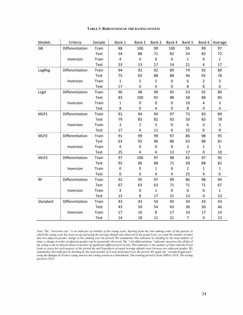
A. Robustness of the rating scale
We construct two indicators of robustness of the rating scale. The first indicator – that we
label “inversion rate” – is an indicator of stability of the rating scale: starting from the risk
ranking order of the quarter at which the rating scale has been set up and using the average
default rate observed at the grade level, we count the number of times that two adjacent grades
change in the ranking over the period. We standardize this indicator by dividing it by the total
number of times a change in order of adjacent grades can be potentially observed. The lower
this indicator is the better the rating scale is. The second indicator – that we label “risk
differentiation” – measures the ability of the rating scale to allocate firms in buckets of
significant differrent level of risk: this indicator is the number of times that the Z-test leads
to reject for each quarter of the period the null hypothesis of equal average default rates
between two adjacent grades. We standardize this indicator by dividing by the total number
of Z-tests performed over the period. The larger this indicator is the better the rating scale is.
These indicators are computed on the calibration sample and on the testing sample for each
bank and each model (see Table 3).
Insert Table 3 here
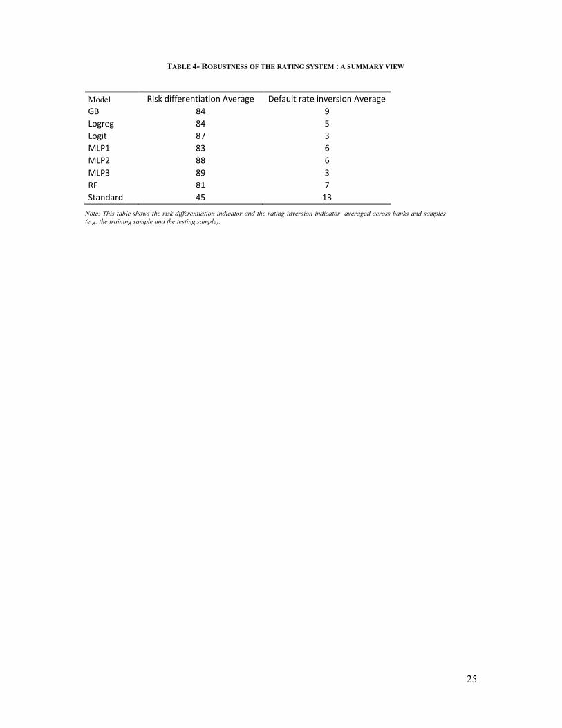
In order to give a summarizing view, we build an aggregate indicator for each of the
model. This indicator is the average of the indicators described in the preceding paragraph
across banks and samples. Therefore an equal weight is put on the performance of the model
on the training sample and on the testing sample on one hand and on each single bank on the
other hand. The highest differentiation of risk is observed for MLP models and the benchmark
model. The lowest inverstion rate is seen for MPL3 and the logistic regression (see Table 4).
The GB and the RF models display very good performances but only on the training period
(see Table 3). Good backtesting results outside the calibration period is key in the validation

15
process and it appears that GB and RF are more likely to fail the validation process along this
dimension. At this point, the models the more likely to lead to a robust rating system are the
benchmark model and the MLPs. However, it is difficult to make a final decision between
the benchmark model and the MLPs : from one bank to another the model the more likely to
meet regulatory expectations is either the neural network model (with one, two or three
hidden layers) or the logistic regression model.
Insert Table 4 here
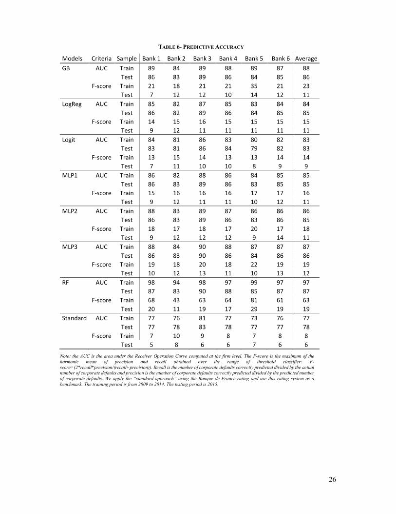
B. Predictive accuracy
We use two indicators for assessing predictive accuracy : the AUC and the F-score. F-score
is the maximum of the harmonic mean of precision and recall obtained over the range of
possible binary classification thresholds :
F-score=(2*recall*precision/(recall+precision))
Where recall is the number of corporate defaults correctly predicted divided by the actual
number of corporate defaults (=TN/(TN+FP)) and precision is the number of corporate defaults
correctly predicted divided by the predicted number of corporate defaults (=TN/(TN+FN)).
Table 5 : Classification table
Model Prediction
Performing Defaulting
Actual Outcome Performing True Positive (TP) False Negative (FN)
Defaulting False Positive (FP) True Negative (TN)
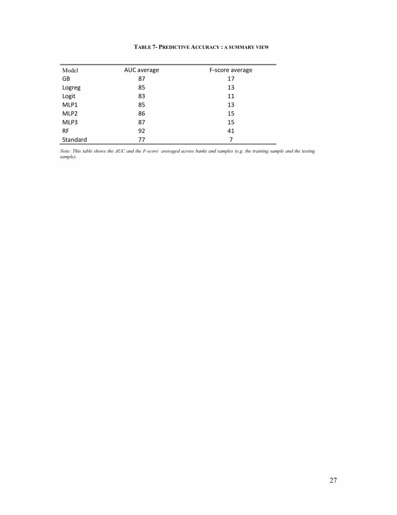
The RF model displays the highest level of AUC and F-score both on the training sample.
However, one should notice the strong decreases in AUC and F-score switching from the
training period to the testing period. These decreases might result from an instability in these
kind of models – overfitting the default rate in the training sample. In addition, we have shown
that this instability of RF models was also an issue for settting up a robust of the rating systems.
Letting aside the RF model, the other models are relatively close both in term of AUC or F-
score and both in sample and out of sample. In sum, the predictive accuracy only does not allow
us to single out a best performing model. This results is consistent with Thomas (2000) or
Baesens et al. (2003) who find that machine learning techniques do not substantially improve
predictive accuracy.28
Insert Table 6 here.
28 Note that an update of this paper (Baesen et al., 2015) also leads to mixed conclusions.
16
C. Measure of capital requirement change
For each model and each bank, we compute the risk weigthed asset (“RWA”) as a share of
the exposure (e.g. the RWA density). For the sake of clarity, we present two levels of RWA :
QQ is the level obtained for the most conservative approach in term of calibration of the PD
(see “point in time and through the cycle conservative PD” in the section D). MM is the level
obtained for the less conservative calibrated PD (“raw PD” in the section D). 29
The GB approach leads to a very strong increase in RWA, leading to a RWA density higher
than the standard approach. RF leads to stong decreases in RWA but only for a sub-sample of
banks. Except for one bank, one the three neural network model displays relative stronger
decrease than the logistic regression models leading to a reduction in RWA Density between
2 and 27 percentage points for the most conservative PD calibration approach. Similar
differences hold for the less conservative approach of PD calibration. In sum, the RWA criteria
allows to single out the MLP models from the benchmark model.
Insert Table 7 here.
IV. Robustness checks and discussion
a. Impact of the sample size on the best performing model
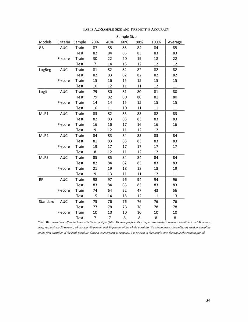
The performance of AI models might be sensitive to sample size. In order to check whether our
results might be driven by sample size, we restrict ourself to the bank with the largest portfolio.
We then perform a comparative analysis between traditional and AI models using respectively
20 percent, 40 percent, 60 percent and 80 percent of the whole portfolio. Coincidently, 20
percent of the largest portfolio is equal to the whole portfolio of the smallest bank. We obtain
these subsambles by random sampling on the firm identifier of the bank portfolio. Once a
counterparty is sampled, it is present in the sample over the whole observation period.
Predictive accuracy is not strongly dependent on the sample size. Whathever the model we
consider, the AUC and the F-score do not change significantly when the sample size increases.
As for the rating system, once again MLP offers the best balance between a low inversion rate
and a strong risk differentiation across all the sample size (see table A.1 and A.2 in appendix
2).
29 Note that results do not substantially change when using the alternative measure of PDs considered in section I.C.b.

17
b. Impact of the discretization of the variables
The AI models that we implement use financial statement variables as continuous variables. By
contrast, before implementing our logistic regressions we proceed to a discretization of the
continuous variable. In order to check whether our results are not driven by this discretization
process, we can compare the AI logreg model to the benchmark model. We note that those two
models are very closed in term of predictive accuracy and robustness of rating system. One
should notice as well that discretization leads to a slight outperformance of the benchmark
model on the testing sample.
c. RWA as the choice variable
One might assume that RWA saving/relief is not the only incentive for a bank to improve
its risk management techniques. A simple framework fo analyzing the value-added of a
classification based algorithm is provided by Khandani et al. (2010) in the case of consumer
credit. Using the notation of the classification table above (see table 5 above) and defining Bd
as the credit exposure at the time of the default, Br the current exposure and Pm the profit margin
rate, one might calcule the profit made by the bank without a forecast model :
Profit without forecast=(TP+FN). Br. Pm-(FP+TN). Bd
Profit with forecast=TP. Br. Pm-FP. Bd- TN. Br
The saving is given by the difference :
TN.( Bd- Br)-FN. Br. Pm
e.g. the saving due to correct decision minus the opportunity cost due to incorrect decision.
This can be simplified further by dividing the saving with the savings that would have been
possible under the perfect-foresight case : all bad customers are correctly identified and their
credit is reduced. Value added is then defined as :
𝑇𝑁 − 𝐹𝑁. 𝑃 .𝐵
(𝐵 − 𝐵 )
𝑇𝑁 + 𝐹𝑃
In our data set, 𝑃 might be proxied by the ratio of interest expenses to total banking debt. We
let this comparison for further work. Note however that for corporate loans, the ability to bank
to cut credit line is less easy than for credit card or consumer loans.
d. AI and explainibility
Finally, another usual critique is that the outcomes of AI models can be harder to explain to non
experts. Going trough validation reports, we observe that the models are mostly challenged by
their performance in their predictive accuracy and in the stability of the induced rating system

18
ex post rather than on the econometrics methodologies or the economic meaning of the input
variables. Therefore at this stage we do not see the lack of “explainability” as hindering the
validation process.
V. Conclusion
In this paper, we compare AI models with the traditional logistic regression used by banks to
set up their internal models of credit risk of corporate businesses. Models are assessed
accordingly to their ability to lead to a rating system and a predictive accuracy that meet the
supervisory expectations such as delineated in the supervisory guide provided to the ECB on
site interal model validation missions.
The MLP and the traditional model lead to the more robust rating system. The RF model
displays by far the highest level of predictive accuracy on the training. However, it displays as
well a strong decreases in this predictive accuracy when we switch from the training sample to
the testing sample. This decrease might result from an instability in these kind of models prone
to an overfitting of the data in the training sample. Putting aside the RF models, there is no
strong difference from a model to another in term of predictive accuracy. Finally, the MLPs are
the model leading to the strongest decrease in capital requirement, leading to a reduction in
RWA density between 2 and 27 percentage points.
Robustness checks show that our results are driven neither by sample size nor by the
difference in processing raw data before implementing the models (discretization in the case of
the traditional model, imputation in the case of the AI models).
Our results show that neural networks provide the strongest incentive for banks to apply AI
models for their internal model of credit risk. Given the legal background of the validation
process, we postulate that the decrease in RWA is the key driver for a bank to adopt a new
model. However, other drivers might be at play –such as P&L measures at the loan level
combined with an ad hoc rule of credit allocation. We let their examination to future work.
19
REFERENCES
Albanesi, Stefania and Vamossy, Domonkos F., Predicting Consumer Default: A Deep Learning
Approach (August 29, 2019). Available at
SSSRN: https://ssrn.com/abstract=3445152 or http://dx.doi.org/10.2139/ssrn.3445152
Amir E. Khandani, Adlar J. Kim, Andrew W. Lo, Consumer credit-risk models via machine-learning
algorithms, Journal of Banking & Finance, Volume 34, Issue 11, 2010, Pages 2767-2787.
Baesens, B, Van Gestel, T, Viaene, S, Stepanova, M, Suykens, J, et Vantienen, J, Benchmarking
state-of-the-art classification algorithms for credit scoring, Journal of the Operational Research
Society, 54 (6), 2003, 627-635.
Behn, Markus and Haselmann, Rainer F. H. and Vig, Vikrant, The Limits of Model-based Regulation
(July 4, 2016). ECB Working Paper No. 1928, Available at SSRN: https://ssrn.com/abstract=2804598
Florentin Butaru, Qingqing Chen, Brian Clark, Sanmay Das, Andrew W. Lo, Akhtar Siddique,
Risk and risk management in the credit card industry, Journal of Banking & Finance, Volume 72,
2016, Pages 218-239.
Fantazzini, D., Figini, S. Random Survival Forests Models for SME Credit Risk Measurement.
Methodol Comput Appl Probab 11, 29–45 (2009).
Flavio Barboza, Herbert Kimura, Edward Altman, Machine learning models and bankruptcy
prediction,Expert Systems with Applications, Volume 83,2017, Pages 405-417,
Hurlin C. and Pérignon, C. (2019), Machine Learning, Nouvelles Données et Scoring de Crédit, Revue
d'Economie Financière, 135, 21-50.
Moscatelli M., Narizzano S., Parlapiano F., Viggiano G. , Corporate default forecasting with
machine learning, Banca d’Italia, Working paper #1256, December 2019.
Plosser M. and J. Santos, Banks’ Incentives and Inconsistent Risk Models, The Review of Financial
Studies, Volume 31, Issue 6, June 2018, Pages 2080–2112.

20
Thomas, L. C., A survey of credit and behavioural scoring : forecasting financial risk of lending to
customers. International Journal of Forecasting, 2000, 16, 179-172.
Larry D. Wall, Some financial regulatory implications of artificial intelligence, Journal of Economics
and Business, Volume 100, 2018, Pages 55-63.
21
FIGURES AND TABLES
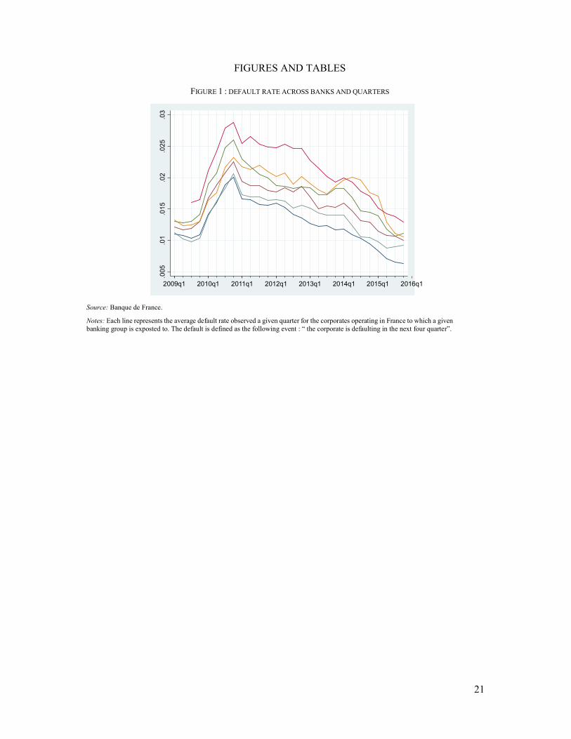
FIGURE 1 : DEFAULT RATE ACROSS BANKS AND QUARTERS
Source: Banque de France.
Notes: Each line represents the average default rate observed a given quarter for the corporates operating in France to which a given banking group is exposted to. The default is defined as the following event : “ the corporate is defaulting in the next four quarter”.
.00
5.0
1.0
15.0
2.0
25.0
3
2009q1 2010q1 2011q1 2012q1 2013q1 2014q1 2015q1 2016q1
22
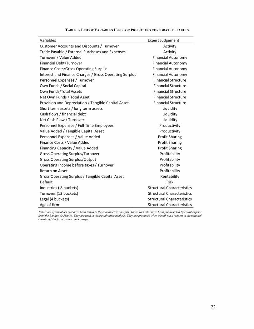
TABLE 1- LIST OF VARIABLES USED FOR PREDICTING CORPORATE DEFAULTS
Variables Expert Judgement Customer Accounts and Discounts / Turnover Activity Trade Payable / External Purchases and Expenses Activity Turnover / Value Added Financial Autonomy Financial Debt/Turnover Financial Autonomy Finance Costs/Gross Operating Surplus Financial Autonomy Interest and Finance Charges / Gross Operating Surplus Financial Autonomy Personnel Expenses / Turnover Financial Structure Own Funds / Social Capital Financial Structure Own Funds/Total Assets Financial Structure Net Own Funds / Total Asset Financial Structure Provision and Depreciation / Tangible Capital Asset Financial Structure Short term assets / long term assets Liquidity Cash flows / financial debt Liquidity Net Cash Flow / Turnover Liquidity Personnel Expenses / Full Time Employees Productivity Value Added / Tangible Capital Asset Productivity Personnel Expenses / Value Added Profit Sharing Finance Costs / Value Added Profit Sharing Financing Capacity / Value Added Profit Sharing Gross Operating Surplus/Turnover Profitability Gross Operating Surplus/Output Profitability Operating Income before taxes / Turnover Profitability Return on Asset Profitability Gross Operating Surplus / Tangible Capital Asset Rentability Default Risk Industries ( 8 buckets) Structural Characteristics Turnover (13 buckets) Structural Characteristics Legal (4 buckets) Structural Characteristics Age of firm Structural Characteristics
Notes: list of variables that have been tested in the econometric analysis. Those variables have been pre-selected by credit experts from the Banque de France. They are used in their qualitative analysis. They are produced when a bank put a request in the national credit register for a given counterparpy.
23
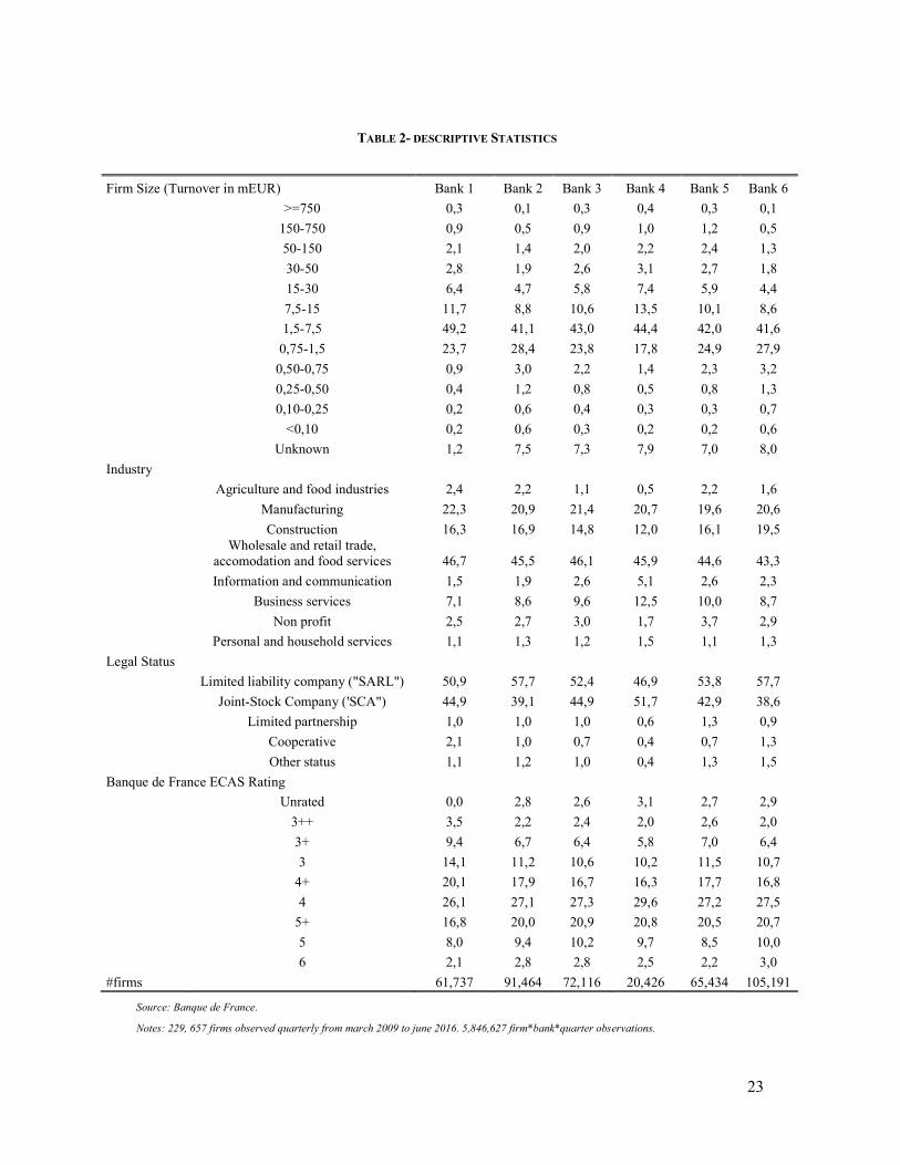
TABLE 2- DESCRIPTIVE STATISTICS
Source: Banque de France.
Notes: 229, 657 firms observed quarterly from march 2009 to june 2016. 5,846,627 firm*bank*quarter observations.
Firm Size (Turnover in mEUR) Bank 1 Bank 2 Bank 3 Bank 4 Bank 5 Bank 6
>=750 0,3 0,1 0,3 0,4 0,3 0,1
150-750 0,9 0,5 0,9 1,0 1,2 0,5
50-150 2,1 1,4 2,0 2,2 2,4 1,3
30-50 2,8 1,9 2,6 3,1 2,7 1,8
15-30 6,4 4,7 5,8 7,4 5,9 4,4
7,5-15 11,7 8,8 10,6 13,5 10,1 8,6
1,5-7,5 49,2 41,1 43,0 44,4 42,0 41,6
0,75-1,5 23,7 28,4 23,8 17,8 24,9 27,9
0,50-0,75 0,9 3,0 2,2 1,4 2,3 3,2
0,25-0,50 0,4 1,2 0,8 0,5 0,8 1,3
0,10-0,25 0,2 0,6 0,4 0,3 0,3 0,7
<0,10 0,2 0,6 0,3 0,2 0,2 0,6
Unknown 1,2 7,5 7,3 7,9 7,0 8,0
Industry
Agriculture and food industries 2,4 2,2 1,1 0,5 2,2 1,6
Manufacturing 22,3 20,9 21,4 20,7 19,6 20,6
Construction 16,3 16,9 14,8 12,0 16,1 19,5
Wholesale and retail trade,
accomodation and food services 46,7 45,5 46,1 45,9 44,6 43,3
Information and communication 1,5 1,9 2,6 5,1 2,6 2,3
Business services 7,1 8,6 9,6 12,5 10,0 8,7
Non profit 2,5 2,7 3,0 1,7 3,7 2,9
Personal and household services 1,1 1,3 1,2 1,5 1,1 1,3
Legal Status
Limited liability company ("SARL") 50,9 57,7 52,4 46,9 53,8 57,7
Joint-Stock Company ('SCA") 44,9 39,1 44,9 51,7 42,9 38,6
Limited partnership 1,0 1,0 1,0 0,6 1,3 0,9
Cooperative 2,1 1,0 0,7 0,4 0,7 1,3
Other status 1,1 1,2 1,0 0,4 1,3 1,5
Banque de France ECAS Rating
Unrated 0,0 2,8 2,6 3,1 2,7 2,9
3++ 3,5 2,2 2,4 2,0 2,6 2,0
3+ 9,4 6,7 6,4 5,8 7,0 6,4
3 14,1 11,2 10,6 10,2 11,5 10,7
4+ 20,1 17,9 16,7 16,3 17,7 16,8
4 26,1 27,1 27,3 29,6 27,2 27,5
5+ 16,8 20,0 20,9 20,8 20,5 20,7
5 8,0 9,4 10,2 9,7 8,5 10,0
6 2,1 2,8 2,8 2,5 2,2 3,0
#firms 61,737 91,464 72,116 20,426 65,434 105,191
24
TABLE 3- ROBUSTNESS OF THE RATING SYSTEM
Models Criteria Sample Bank 1 Bank 2 Bank 3 Bank 4 Bank 5 Bank 6 Average GB Differentiation Train 88 100 99 100 95 99 97 Test 54 88 71 82 54 83 72 Inversion Train 4 0 0 0 1 0 1 Test 33 13 17 14 21 4 17 LogReg Differentiation Train 94 92 92 89 74 92 89 Test 75 83 88 88 46 92 78 Inversion Train 1 5 5 0 6 2 3 Test 17 0 4 0 8 8 6 Logit Differentiation Train 96 98 99 95 53 92 89 Test 83 100 92 88 58 88 85 Inversion Train 1 0 0 0 10 4 3 Test 8 0 4 0 8 4 4 MLP1 Differentiation Train 91 94 94 97 73 83 89 Test 79 83 82 92 50 83 78 Inversion Train 3 2 3 0 6 3 3 Test 17 4 11 0 25 0 9 MLP2 Differentiation Train 91 99 99 97 86 98 95 Test 63 92 96 88 63 88 81 Inversion Train 4 0 0 0 2 1 1 Test 25 4 4 13 17 0 10 MLP3 Differentiation Train 97 100 97 98 83 97 95 Test 92 96 88 71 58 88 82 Inversion Train 0 0 1 0 2 1 1 Test 0 0 4 4 25 4 6 RF Differentiation Train 92 95 97 99 86 98 94 Test 67 63 63 71 71 71 67 Inversion Train 3 0 1 0 0 0 1 Test 13 8 17 21 13 4 13 Standard Differentiation Train 43 43 54 45 34 43 43 Test 43 50 54 43 36 50 46 Inversion Train 17 16 8 17 10 17 14 Test 14 18 11 21 7 4 13
Note: The “inversion rate” is an indicator of stability of the rating scale. Starting from the risk ranking order of the quarter at which the rating scale has been set up and using the average default rate observed at the grade level, we count the number of times that two adjacent grades change in the ranking over the period. We standardize this indicator by dividing by the total number of times a change in order of adjacent grades can be potentially observed. The “risk differentiation” indicator measures the ability of the rating scale to allocate firms in buckets of significant different level of risk. This indicator is the number of times that the Z-test leads to reject for each quarter of the period the null hypothesis of equal average default rates between two adjacent grades. We standardize this indicator by dividing by the total number of Z-tests performed over the period. We apply the “standard approach” using the Banque de France rating and use this rating system as a benchmark. The training period is from 2009 to 2014. The testing period is 2015.
25
TABLE 4- ROBUSTNESS OF THE RATING SYSTEM : A SUMMARY VIEW
Model Risk differentiation Average Default rate inversion Average GB 84 9 Logreg 84 5 Logit 87 3 MLP1 83 6 MLP2 88 6 MLP3 89 3 RF 81 7 Standard 45 13
Note: This table shows the risk differentiation indicator and the rating inversion indicator averaged across banks and samples (e.g. the training sample and the testing sample).
26
TABLE 6- PREDICTIVE ACCURACY
Models Criteria Sample Bank 1 Bank 2 Bank 3 Bank 4 Bank 5 Bank 6 Average GB AUC Train 89 84 89 88 89 87 88 Test 86 83 89 86 84 85 86 F-score Train 21 18 21 21 35 21 23 Test 7 12 12 10 14 12 11 LogReg AUC Train 85 82 87 85 83 84 84 Test 86 82 89 86 84 85 85 F-score Train 14 15 16 15 15 15 15 Test 9 12 11 11 11 11 11 Logit AUC Train 84 81 86 83 80 82 83 Test 83 81 86 84 79 82 83 F-score Train 13 15 14 13 13 14 14 Test 7 11 10 10 8 9 9 MLP1 AUC Train 86 82 88 86 84 85 85 Test 86 83 89 86 83 85 85 F-score Train 15 16 16 16 17 17 16 Test 9 12 11 11 10 12 11 MLP2 AUC Train 88 83 89 87 86 86 86 Test 86 83 89 86 83 86 85 F-score Train 18 17 18 17 20 17 18 Test 9 12 12 12 9 14 11 MLP3 AUC Train 88 84 90 88 87 87 87 Test 86 83 90 86 84 86 86 F-score Train 19 18 20 18 22 19 19 Test 10 12 13 11 10 13 12 RF AUC Train 98 94 98 97 99 97 97 Test 87 83 90 88 85 87 87 F-score Train 68 43 63 64 81 61 63 Test 20 11 19 17 29 19 19 Standard AUC Train 77 76 81 77 73 76 77 Test 77 78 83 78 77 77 78 F-score Train 7 10 9 8 7 8 8 Test 5 8 6 6 7 6 6
Note: the AUC is the area under the Receiver Operation Curve computed at the firm level. The F-score is the maximum of the harmonic mean of precision and recall obtained over the range of threshold classifier: F-score=(2*recall*precision/(recall+precision)). Recall is the number of corporate defaults correctly predicted divided by the actual number of corporate defaults and precision is the number of corporate defaults correctly predicted divided by the predicted number of corporate defaults. We apply the “standard approach” using the Banque de France rating and use this rating system as a benchmark. The training period is from 2009 to 2014. The testing period is 2015.
27
TABLE 7- PREDICTIVE ACCURACY : A SUMMARY VIEW
Model AUC average F-score average GB 87 17 Logreg 85 13 Logit 83 11 MLP1 85 13 MLP2 86 15 MLP3 87 15 RF 92 41 Standard 77 7
Note: This table shows the AUC and the F-score averaged across banks and samples (e.g. the training sample and the testing sample).
28
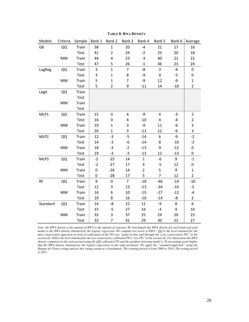
TABLE 8- RWA DENSITY
Models Criteria Sample Bank 1 Bank 2 Bank 3 Bank 4 Bank 5 Bank 6 Average GB QQ Train 38 1 20 -4 21 17 16
Test 41 2 24 -2 25 20 18
MM Train 44 4 23 -3 40 21 22 Test 47 5 26 -1 46 23 24 LogReg QQ Train 3 1 7 -8 3 -4 0
Test 3 1 8 -9 4 -5 0
MM Train 5 1 7 -9 12 -9 1 Test 5 2 9 -11 14 -10 2 Logit QQ Train
Test
MM Train Test MLP1 QQ Train 15 0 4 -9 4 -3 2
Test 16 0 4 -10 4 -4 2
MM Train 19 1 3 -9 11 -6 3 Test 20 1 3 -11 12 -6 3 MLP2 QQ Train 12 -3 -5 -14 6 -9 -2
Test 14 -3 -6 -14 8 -10 -2
MM Train 18 -3 -2 -13 9 -12 0 Test 19 -3 -3 -13 12 -13 0 MLP3 QQ Train -2 -25 14 1 -6 9 -1
Test -2 -27 17 4 -5 12 0
MM Train 0 -26 14 2 5 9 1 Test 0 -28 17 5 7 12 2 RF QQ Train 9 0 7 -18 -46 -14 -10
Test 12 3 13 -13 -34 -10 -5
MM Train 16 6 10 -15 -27 -12 -4 Test 19 8 16 -10 -14 -8 2 Standard QQ Train 14 -8 22 11 -9 8 6
Test 15 -5 27 16 -4 9 10
MM Train 32 3 37 25 24 20 23
Test 32 7 41 29 30 22 27
Note: the RWA density is the amount of RWA to the amount of exposure We benchmark this RWA density for each bank and each model to the RWA density obtained for the logistic regression. We compute two levels of RWA : QQ is the level obtained for the most conservative approach in term of calibration of the PD (see “point in time and through the cycle conservative PD” in the section D). MM is the level obtained for the less conservative calibrated PD (“raw PD” in the section D). For illustration the RWA density computed on the train period using the QQ calibrated PD and the gradient boosting model is 38 percentage point higher that the RWA density obtained for the logistic regression on the same perimeter. We apply the “standard approach” using the Banque de France rating and use this rating system as a benchmark. The training period is from 2009 to 2014. The testing period is 2015.

29
Appendix 1 : learning strategies for AI binary classifiers
In order to determine optimal hyper-parameters during the training phase of the different
models on each dataset (one for each bank), we performed a grid search to explore different
possible hyper-parameters values, and cross-validation to determine the optimal value in each
case.
The cross-validation strategy is based on a 6-fold chronological split (the training datasets
cover 24 quarters corresponding to 6 years of quarterly observations) which means that for each
set of hyper-parameters values fixed when performing the grid search, the model is trained 6
times on 5 years of data and evaluated each time on the remaining year of observation taken
out of the training sample as a validation set.
The evaluation metric used to select the optimal values of the hyper-parameters is the AUC,
which means that they will be set to the values that lead to the best average AUC over the 6
validation sets. Once those values are determined, the model is trained over the whole training
set with its hyper-parameters fixed accordingly.
The exploration space has been fixed specifically for each model architecture (however, it is
not varying from one bank to another for a given architecture) according to their specificities
and empirical appreciation. When several hyper-parameters have been fine-tuned, the
exploration space consists in the Cartesian product of the sets of values explored for each hyper-
parameter. The following table denotes those exploration spaces, using sklearn’s hyper-
parameters notations.
Architecture Fixed hyper-parameters (when different than default sklearn value) Exploration space for grid search
LogReg C = {10-i/3 | -6≤i<10}
MLP1 hidden_layer_sizes = (2) solver = 'lbfgs'
alpha = {10i/2 | 4≤i<8} random_state = {i1,…,i8}
MLP2 hidden_layer_sizes = (4, 2) solver = 'lbfgs'
alpha = {10i/2 | 4≤i<8} random_state = {i1,…,i8}
MLP3 hidden_layer_sizes = (8, 4, 2) solver = 'lbfgs'
alpha = {10i/2 | 4≤i<8} random_state = {i1,…,i8}
RF n_estimators = 32 max_depth = {4, 5, 6, 7, 8, 9, 10, 11}
GB n_estimators = 64 max_depth = {1, 2, 3, 4} random_state = {i1,…,i8}

30
31
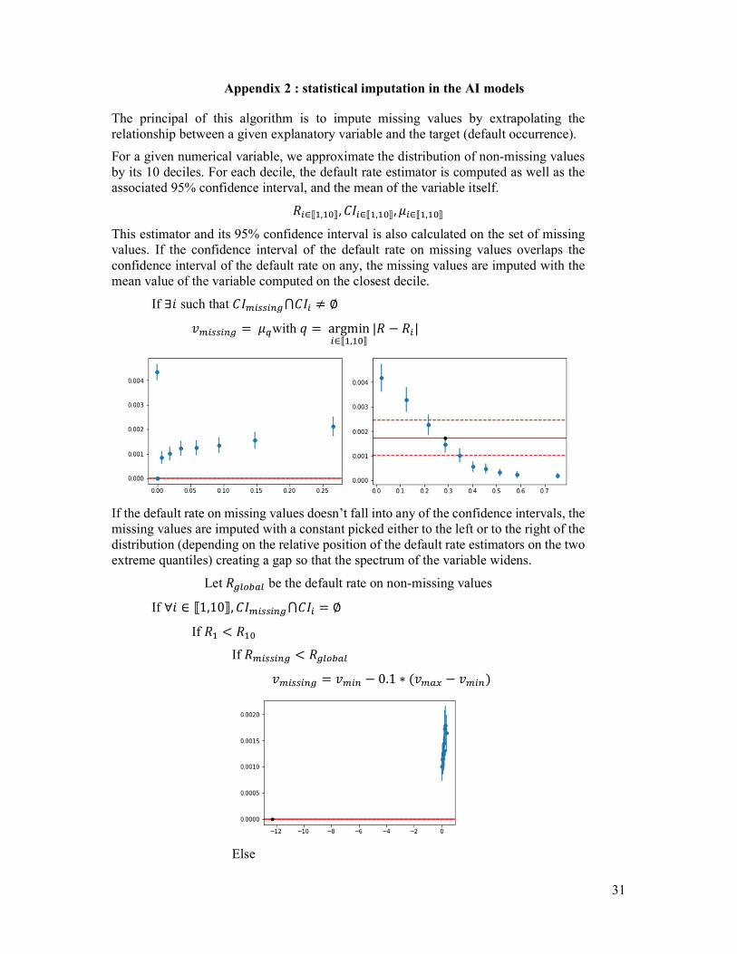
Appendix 2 : statistical imputation in the AI models
The principal of this algorithm is to impute missing values by extrapolating the relationship between a given explanatory variable and the target (default occurrence).
For a given numerical variable, we approximate the distribution of non-missing values by its 10 deciles. For each decile, the default rate estimator is computed as well as the associated 95% confidence interval, and the mean of the variable itself.
𝑅 ∈⟦ , ⟧, 𝐶𝐼 ∈⟦ , ⟧, 𝜇 ∈⟦ , ⟧
This estimator and its 95% confidence interval is also calculated on the set of missing values. If the confidence interval of the default rate on missing values overlaps the confidence interval of the default rate on any, the missing values are imputed with the mean value of the variable computed on the closest decile.
If ∃𝑖 such that 𝐶𝐼 ⋂𝐶𝐼 ≠ ∅
𝑣 = 𝜇 with 𝑞 = argmin∈⟦ , ⟧
|𝑅 − 𝑅 |
If the default rate on missing values doesn’t fall into any of the confidence intervals, the missing values are imputed with a constant picked either to the left or to the right of the distribution (depending on the relative position of the default rate estimators on the two extreme quantiles) creating a gap so that the spectrum of the variable widens.
Let 𝑅 be the default rate on non-missing values
If ∀𝑖 ∈ ⟦1,10⟧, 𝐶𝐼 ⋂𝐶𝐼 = ∅
If 𝑅 < 𝑅
If 𝑅 < 𝑅
𝑣 = 𝑣 − 0.1 ∗ (𝑣 − 𝑣 )
Else
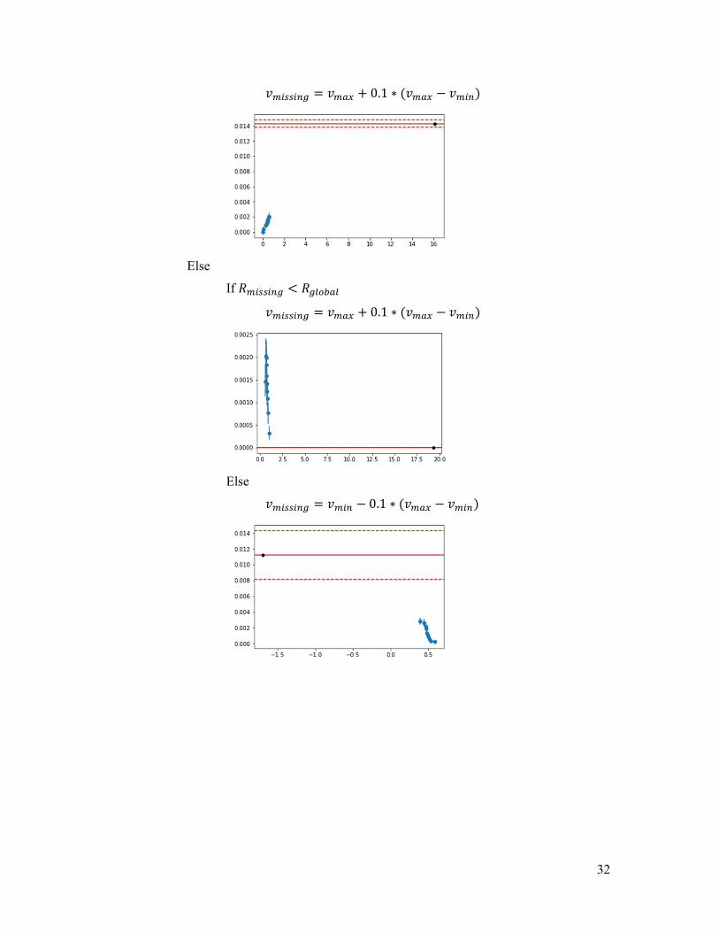
32
𝑣 = 𝑣 + 0.1 ∗ (𝑣 − 𝑣 )
Else
If 𝑅 < 𝑅
𝑣 = 𝑣 + 0.1 ∗ (𝑣 − 𝑣 )
Else
𝑣 = 𝑣 − 0.1 ∗ (𝑣 − 𝑣 )
33
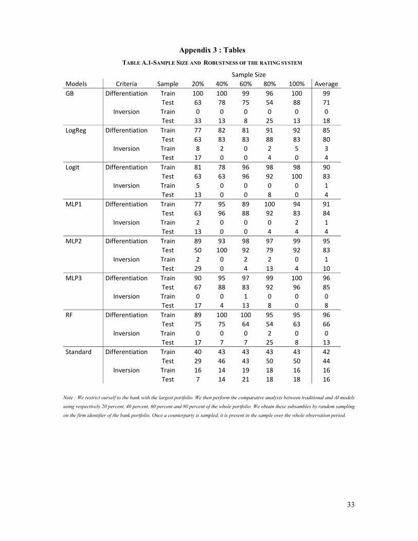
Appendix 3 : Tables
TABLE A.1-SAMPLE SIZE AND ROBUSTNESS OF THE RATING SYSTEM
Sample Size Models Criteria Sample 20% 40% 60% 80% 100% Average GB Differentiation Train 100 100 99 96 100 99 Test 63 78 75 54 88 71 Inversion Train 0 0 0 0 0 0 Test 33 13 8 25 13 18 LogReg Differentiation Train 77 82 81 91 92 85 Test 63 83 83 88 83 80 Inversion Train 8 2 0 2 5 3 Test 17 0 0 4 0 4 Logit Differentiation Train 81 78 96 98 98 90 Test 63 63 96 92 100 83 Inversion Train 5 0 0 0 0 1 Test 13 0 0 8 0 4 MLP1 Differentiation Train 77 95 89 100 94 91 Test 63 96 88 92 83 84 Inversion Train 2 0 0 0 2 1 Test 13 0 0 4 4 4 MLP2 Differentiation Train 89 93 98 97 99 95 Test 50 100 92 79 92 83 Inversion Train 2 0 2 2 0 1 Test 29 0 4 13 4 10 MLP3 Differentiation Train 90 95 97 99 100 96 Test 67 88 83 92 96 85 Inversion Train 0 0 1 0 0 0 Test 17 4 13 8 0 8 RF Differentiation Train 89 100 100 95 95 96 Test 75 75 64 54 63 66 Inversion Train 0 0 0 2 0 0 Test 17 7 7 25 8 13 Standard Differentiation Train 40 43 43 43 43 42 Test 29 46 43 50 50 44 Inversion Train 16 14 19 18 16 16 Test 7 14 21 18 18 16
Note : We restrict ourself to the bank with the largest portfolio. We then perform the comparative analysis between traditional and AI models
using respectively 20 percent, 40 percent, 60 percent and 80 percent of the whole portfolio. We obtain these subsambles by random sampling
on the firm identifier of the bank portfolio. Once a counterparty is sampled, it is present in the sample over the whole observation period.
34
TABLE A.2-SAMPLE SIZE AND PREDICTIVE ACCURACY
Sample Size Models Criteria Sample 20% 40% 60% 80% 100% Average GB AUC Train 87 85 85 84 84 85 Test 82 84 83 83 83 83 F-score Train 30 22 20 19 18 22 Test 7 14 13 12 12 12 LogReg AUC Train 81 82 82 82 82 82 Test 82 83 82 82 82 82 F-score Train 15 16 15 15 15 15 Test 10 12 11 11 12 11 Logit AUC Train 79 80 81 80 81 80 Test 79 82 80 80 81 80 F-score Train 14 14 15 15 15 15 Test 10 11 10 11 11 11 MLP1 AUC Train 83 82 83 83 82 83 Test 82 83 83 83 83 83 F-score Train 16 16 17 16 16 16 Test 9 12 11 12 12 11 MLP2 AUC Train 84 83 84 83 83 84 Test 81 83 83 83 83 83 F-score Train 19 17 17 17 17 17 Test 8 12 11 12 12 11 MLP3 AUC Train 85 85 84 84 84 84 Test 82 84 82 83 83 83 F-score Train 21 19 18 18 18 19 Test 9 13 11 11 12 11 RF AUC Train 98 97 96 94 94 96 Test 83 84 83 83 83 83 F-score Train 74 64 52 47 43 56 Test 15 14 15 12 11 13 Standard AUC Train 75 76 76 76 76 76 Test 77 78 78 78 78 78 F-score Train 10 10 10 10 10 10 Test 7 7 8 8 8 8
Note : We restrict ourself to the bank with the largest portfolio. We then perform the comparative analysis between traditional and AI models
using respectively 20 percent, 40 percent, 60 percent and 80 percent of the whole portfolio. We obtain these subsambles by random sampling
on the firm identifier of the bank portfolio. Once a counterparty is sampled, it is present in the sample over the whole observation period.