Revealed preferences over risk and uncertainty

IFS Working Paper W15/25

Matthew PolissonJohn QuahLudovic Renou

The Institute for Fiscal Studies (IFS) is an independent research institute whose remit is to carry out rigorous economic research into public policy and to disseminate the findings of this research. IFS receives generous support from the Economic and Social Research Council, in particular via the ESRC Centre for the Microeconomic Analysis of Public Policy (CPP). The content of our working papers is the work of their authors and does not necessarily represent the views of IFS research staff or affiliates.

Revealed preferences over risk and uncertainty

Matthew Polisson, John K.-H. Quah, and Ludovic Renou�

September 12, 2015

Abstract: Consider a finite data set where each observation consists of a bundle of

contingent consumption chosen by an agent from a constraint set of such bundles.

We develop a general procedure for testing the consistency of this data set with a

broad class of models of choice under risk and under uncertainty. Unlike previous

work, we do not require that the agent has a convex preference, so we allow for risk

loving and elation seeking behavior. Our procedure can also be extended to calculate

the magnitude of violations from a particular model of choice, using an index first

suggested by Afriat (1972, 1973). We then apply this index to evaluate different models

(including expected utility and disappointment aversion) in the data collected by Choi

et al. (2007). We show that among those subjects exhibiting choice behavior consistent

with the maximization of some increasing utility function, more than half are consistent

with models of expected utility and disappointment aversion.

Keywords: expected utility, rank dependent utility, maxmin expected utility, varia-

tional preferences, generalized axiom of revealed preference

JEL classification numbers: C14, C60, D11, D12, D81

� Email addresses: matthew.polisson@le.ac.uk; john.quah@economics.ox.ac.uk; lrenou@essex.ac.uk.

This research made use of the ALICE High Performance Computing Facility at the University of Leicester.

Part of this research was carried out while Matthew Polisson was a Visiting Associate at Caltech and while

Ludovic Renou was a Visiting Professor at the University of Queensland, and they would like to thank

these institutions for their hospitality and support. We are grateful to Don Brown, Ray Fisman, Felix

Kubler, Shachar Kariv, and Collin Raymond for helpful discussions and comments, as well as to seminar

audiences at Adelaide, Brown, Caltech, Leicester, NUS, NYU Stern, Oxford, PSE, Toulouse, UC Irvine,

UCSD, Queensland, and QUT, and to conference participants at the 2014 Canadian Economic Association

Annual Conference (Simon Fraser), the 2014 North American Summer Meeting of the Econometric Society

(Minnesota), the 2014 SAET Conference (Waseda), the 2014 Workshop on Nonparametric Demand (IFS

and CeMMAP), the 2014 Dauphine Workshop in Economic Theory, the 2015 Australasian Economic Theory

Workshop (Deakin), the 2015 Bath Economic Theory Workshop, the 2015 Canadian Economic Theory

Conference (Western Ontario), the 2015 ESRC Workshop on Decision Theory and Applications (Essex), the

2015 Cowles Summer Conference on Heterogeneous Agents and Microeconometrics (Yale), the 2015 SAET

Conference (Cambridge), and the 2015 Econometric Society World Congress (Montreal).

1

1. Introduction

Let O � tppt, xtquTt�1 be a finite set, where pt P Rs�� and xt P Rs

�. We interpret O

as a set of observations, where xt is the observed bundle of s goods chosen by an agent

(the demand bundle) at the price vector pt. A utility function U : Rs� Ñ R is said to

rationalize O if, at every observation t, xt is the bundle that maximizes U in the budget set

Bt � tx P Rs� : pt �x ¤ pt �xtu. For any data set that is rationalizable by a locally nonsatiated

utility function, its revealed preference relations must satisfy a no-cycling condition called

the generalized axiom of revealed preference (GARP). Afriat’s (1967) Theorem shows that

any data set that obeys GARP will in turn be rationalizable by a utility function that is

continuous, strictly increasing, and concave. This result is very useful because it provides a

nonparametric test of utility maximization that can be readily implemented in observational

and experimental settings. It is computationally straightforward to check GARP directly;

alternatively, GARP holds if and only if there is a solution to a set of linear inequalities

constructed from the data and one could also check if this system has a solution.1

It is both useful and natural to develop tests, similar to the one developed by Afriat,

for alternative hypotheses on agent behavior. Our objective in this paper is to develop

a procedure that is useful for testing models of choice under risk and under uncertainty.

Retaining the formal setting described in the previous paragraph, we can interpret s as the

number of states of the world, with xt a bundle of contingent consumption, and pt the state

prices faced by the agent. In a setting like this, we can ask what conditions on the data

set are necessary and sufficient for it to be consistent with an agent who is maximizing

an expected utility function. This means that xt maximizes the agent’s expected utility,

compared to other bundles in the budget set. Assuming that the probability of state s is

commonly known to be πs, this involves recovering a Bernoulli function u : R� Ñ R, which

we require to be continuous and strictly increasing, so that, for each t � 1, 2, . . . , T ,

s

s�1

πsupxtsq ¥

s

s�1

πsupxsq for all x P Bt. (1)

1 For proofs of Afriat’s Theorem, see Afriat (1967), Diewert (1973), Varian (1982), and Fostel, Scarf,

and Todd (2004). The term GARP is from Varian (1982); Afriat refers to the same property as cyclical

consistency.

2

In the case where the state probabilities are subjective and unknown to the observer, it

would be necessary to recover both u and tπsuss�1 so that (1) holds.

In fact, tests of this sort have already been developed by Varian (1983a, 1983b, 1988)

and Green and Srivastava (1986). Such tests involve solving a set of inequalities that are

derived from the data; there is consistency with expected utility maximization if and only if

a solution to these inequalities exists. However, these results (and later generalizations and

variations, including those on other models of choice under risk and under uncertainty2) rely

on two crucial assumptions: (1) the agent’s utility function is concave, and (2) the budget set

Bt takes the classical form defined above, where prices are linear and markets are complete.

These two assumptions guarantee that the first order conditions are necessary and sufficient

for optimality and can in turn be converted into a necessary and sufficient test. The use of

concavity to simplify the formulation of revealed preference tests is well known and can be

applied to models of choice in other contexts (see Diewert (2012)).

Our contribution in this paper is to develop a testing procedure that has the following

features: (i) it is potentially adaptable to test for different models of choice under risk and

under uncertainty, and not just the expected utility model; (ii) it is a ‘pure’ test of a given

model as such and does not require the a priori exclusion of certain ‘behavioral’ phenomena,

such as risk loving or elation seeking or reference point effects, that lead to a nonconcave

Bernoulli utility function, or more generally, nonconvex preferences over contingent con-

sumption; (iii) it is applicable to situations with complex budgetary constraints and can be

employed even when there is market incompleteness or when there are nonconvexities in the

budget set due to nonlinear pricing or other practices;3 and (iv) it can be easily adapted

to measure ‘near’ rationalizability (using the indices developed by Afriat (1972, 1973) and

Varian (1990)) in cases where the data set is not exactly rationalizable by a particular model.

In the case of objective expected utility maximization, a data set is consistent with

this model if and only if there is a solution to a set of linear inequalities. In the case

of, for example, subjective expected utility, rank dependent utility, or maxmin expected

utility, our test involves solving a finite set of bilinear inequalities that is constructed from

2 See Diewert (2012), Bayer et al. (2013), Kubler, Selden, and Wei (2014), Echenique and Saito (2015),

Chambers, Liu, and Martinez (2015), and Chambers, Echenique, and Saito (2015).3 For an extension Afriat’s Theorem to nonlinear budget constraints, see Forges and Minelli (2009).

3

the data. These problems are decidable, in the sense that there is a known algorithm

that can determine in a finite number of steps whether or not a solution exists. Nonlinear

tests are not new to the revealed preference literature; for example, they appear in tests of

weak separability (Varian, 1983a), in tests of maxmin expected utility and other models of

ambiguity (Bayer et al., 2013), and in tests of Walrasian general equilibrium (Brown and

Matzkin, 1996). Solving such problems can be computationally demanding, but certain cases

can be computationally straightforward because of certain special features and/or when the

number of observations is small.4 In the case of the tests that we develop, they simplify

dramatically and are implementable in practice when there are only two states (though they

remain nonlinear). The two-state case, while special, is very common in applied theoretical

settings and laboratory experiments.5

1.1 The lattice test procedure

We now give a brief description of our test. Given a data set O � tppt, xtquTt�1, we

define the discrete consumption set X � tx1 P R� : x1 � xts for some t, su Y t0u. Besides

zero, X contains those levels of consumption that were chosen at some observation and at

some state. Since O is finite, so is X , and its product L � X s forms a grid of points in

Rs�; in formal terms, L is a finite lattice. For example, Figure 1 depicts a data set where

x1 � p2, 5q at p1 � p5, 2q, x2 � p6, 1q at p2 � p1, 2q, and x3 � p4, 3q at p3 � p4, 3q. In this

case, X � t0, 1, 2, 3, 4, 5, 6u and L � X � X .

Suppose we would like to test whether O is consistent with expected utility maximization

given objective probabilities tπsuss�1 that are known to us. Clearly, a necessary condition for

this to hold is that we can find a set of real numbers tuprqurPX with the following properties:

(i) upr2q ¡ upr1q whenever r2 ¡ r1, and (ii) for every t � 1, 2, . . . , T ,

s

s�1

πsupxtsq ¥

s

s�1

πsupxsq for all x P Bt X L, (2)

4 It is not uncommon to perform tests on fewer than 20 observations. This is partly because revealed

preference tests do not in general account for errors, which are unavoidable across many observations.5 While we have not found it necessary to use them in our implementation in this paper, there are solvers

available for mixed integer nonlinear programs (for example, as surveyed in Bussieck and Vigerske (2010))

that are potentially useful for implementing bilinear tests more generally.

4

0

1

2

3

4

5

6

7

8

9

10

0 1 2 3 4 5 6 7 8 9 10

x1

x2

Figure 1: Constructing the finite lattice

with the inequality strict whenever x P Bt X L and x is in the interior of the budget set Bt.

Since X is finite, the existence of tuprqurPX with properties (i) and (ii) can be straightfor-

wardly ascertained by solving a family of linear inequalities. Our main result says that if a

solution can be found, then there is a Bernoulli function u : R� Ñ R that extends tuprqurPX

and satisfies (1). Returning to the example depicted in Figure 1, suppose we know that

π1 � π2 � 0.5. Our test requires that we find uprq, for r � 0, 1, 2, . . . , 6, such that the

expected utility of the chosen bundle pxt1, xt2q is (weakly) greater than that of any lattice

points within the corresponding budget set Bt. One could check that these requirements

are satisfied for uprq � r, for r � 0, 1, . . . , 6, so we conclude that the data set is consistent

with expected utility maximization. A detailed explanation of our testing procedure and its

application to the expected utility model is found in Section 2. Section 3 shows how this

procedure can be applied to test for other models of choice under risk and under uncertainty,

including rank dependent utility, choice acclimating personal equilibrium, maxmin expected

utility, and variational preferences.

1.2 Empirical implementation

To illustrate the use of these tests, we implement them in Section 5 on a data set ob-

tained from the portfolio choice experiment in Choi et al. (2007). In this experiment, each

5

subject was asked to purchase Arrow-Debreu securities under different budget constraints.

There were two states of the world and it was commonly known that states occurred either

symmetrically (each with probability 1/2) or asymmetrically (one with probability 1/3 and

the other with probability 2/3). In their analysis, Choi et al. (2007) first performed GARP

tests on the data; subjects who passed or came very close to passing (and whose behavior

was therefore broadly consistent with the maximization of an increasing utility function)

were then fitted to a parameterized model of disappointment aversion.

In our analysis, we test four utility-maximizing models on the data, using a nonparamet-

ric approach throughout. In decreasing order of generality, the models are increasing utility,

stochastically monotone utility, disappointment aversion, and expected utility. Consistency

with the increasing utility model can be verified by checking GARP. By stochastically mono-

tone utility, we mean that the utility function is strictly increasing with respect to first order

stochastic dominance; this hypothesis is stronger than saying that the utility function is

strictly increasing and it can be tested via a stronger version of GARP recently formulated

by Nishimura, Ok, and Quah (2015).6 Lastly, the tools developed in this paper allow us to

test the disappointment aversion and expected utility models.

Given that there are 50 observations on every subject, it is not empirically meaningful to

simply carry out exact tests, because the overwhelming majority of subjects are likely to fail

even the GARP test (which is the most permissive of the four). What is required is a way of

measuring how close each subject is to being consistent with a particular model of behavior.

In the case of the increasing utility model, Choi et al. (2007) measured this gap using the

critical cost efficiency index (CCEI). This index was first proposed by Afriat (1972, 1973)

who also showed how GARP can be modified to calculate the index. We extend this approach

by calculating CCEIs for all four models of interest. Not all revealed preference tests can

be straightforwardly adapted to perform CCEI calculations; the fact that it is possible to

modify our tests of the disappointment aversion and expected utility models for this purpose

is one of its important features and is due to the fact that these tests can be performed

6 When the two states are equiprobable, a utility function is stochastically monotone if and only if it is

strictly increasing and symmetric. If state 1 has a probability 2/3, then the utility function U is stochastically

monotone if and only if it is strictly increasing and Upa, bq ¡ Upb, aq whenever a ¡ b. See Section 5 for

details.

6

on nonconvex budget sets. We explain this in greater detail in Section 4, which discusses

CCEIs. We also determine the power (Bronars, 1987) of each model, i.e. the probability of

a random data set being inconsistent with that model (at a given efficiency threshold). This

information allows us to rank the performance of each model using Selten’s (1991) index of

predictive success. This index balances the success of a model in predicting observations

(which favors the increasing utility model since it is the most permissive) with the specificity

of its predictions (which favors expected utility since it is the most restrictive).

Our main findings are as follows. (i) In the context of the Choi et al. (2007) experiment,

all four models have high power in the sense that the probability of a randomly drawn data

set being consistent with the model is close to zero. (ii) Measured by the Selten index,

the best performing model is increasing utility, followed by stochastically monotone utility,

disappointment aversion, and expected utility. In other words, the greater success that the

increasing utility model has in explaining a set of observations more than compensates for its

relative lack of specificity. That said, all four models have considerable success in explaining

the data; for example, at an efficiency level of 0.9, the pass rates of the four models are 81%,

68%, 54%, and 52%, respectively. (iii) Conditioning on agents who pass GARP (at or above

some efficiency level, say 0.9), both disappointment aversion and expected utility remain

very precise, i.e., the probability of a randomly drawn data set satisfying disappointment

aversion (and hence expected utility), conditional on it passing GARP, is also very close

to zero. (iv) On the other hand, more than half of the subjects who pass GARP are also

consistent with the disappointment aversion and expected utility models, which gives clear

support for these models in explaining the behavior of agents who are (in the first place)

maximizing some increasing utility function.

2. Testing the model on a lattice

We assume that there is a finite set of states, denoted by S � t1, 2, . . . , su. The contingent

consumption space is Rs�; for a typical consumption bundle x P Rs

�, the sth entry, xs, specifies

the consumption level in state s.7 We assume that there are T observations in the data set

7 Our results do depend on the realization in each state being one-dimensional (which can be interpreted

as a monetary payoff, but not a bundle of goods). This case is the one most often considered in applications

and experiments and is also the assumption in a number of recent papers, including Kubler, Selden, and

7

O, where O � tpxt, BtquTt�1. This means that the agent is observed to have chosen the

bundle xt from the set Bt � Rs�. We assume that Bt is compact and that xt P BBt, where

BBt denotes the upper boundary of Bt. An element y P Bt is in BBt if there is no x P Bt such

that x ¡ y.8,9 The most important example of Bt is the standard budget set when markets

are complete, i.e.,

Bt � tx P Rs� : pt � x ¤ pt � xtu, (3)

with pt " 0 being the vector of state prices. Our formulation also allows for the market

to be incomplete. Suppose that the agent’s contingent consumption is achieved through a

portfolio of securities and that the asset prices do not admit arbitrage; then it is well known

that there exists a price vector pt " 0 such that

Bt � tx P Rs� : pt � x ¤ pt � xtu X tZ � ωu,

where Z is the span of assets available to the agent and ω is his endowment of contingent

consumption. Note that both Bt and xt will be known to the observer so long as he can

observe the asset prices and the agent’s holding of securities, the asset payoffs in every state,

and the agent’s endowment of contingent consumption, ω.

Let tφp�, tquTt�1 be a collection of functions, where φp�, tq : Rs� Ñ R is continuous and

strictly increasing.10 The data set O � tpxt, BtquTt�1 is said to be rationalizable by tφp�, tquTt�1

if there exists a continuous and strictly increasing function u : R� Ñ R�, which we shall

refer to as the Bernoulli function, such that

φpupxtq, tq ¥ φpupxq, tq for all x P Bt, (4)

where upxq � pupx1q, upx2q, . . . , upxsqq. In other words, xt is an optimal choice in Bt, assum-

ing that the agent is maximizing φpupxq, tq. It is natural to require u to be strictly increasing

since we typically interpret its argument to be money. The requirements on u guarantee that

φpupxq, tq is continuous and strictly increasing in x, so that this model is a special case of

Wei (2014), Echenique and Saito (2015), and Chambers, Echenique, and Saito (2015). The papers by Varian

(1983), Green and Srivastava (1986), Bayer et al. (2013), and Chambers, Liu, and Martinez (2015) allow for

multi-dimensional realizations but they also require the convexity of the agent’s preference over contingent

consumption and linear budget sets.8For vectors x, y P Rs, x ¡ y if x � y and xi ¥ yi for all i. If xi ¡ yi for all i, we write x " y.9For example, if Bt � tpx, yq P R2

�: px, yq ¤ p1, 1qu, then p1, 1q P BBt but p1, 1{2q R BBt.

10By strictly increasing, we mean that φpz, tq ¡ φpz1, tq if z ¡ z1.

8

the increasing utility model. The continuity of the utility function is an important property,

because it guarantees that the agent’s utility maximization problem always has a solution

on a compact constraint set.11 Many of the basic models of choice under risk and under

uncertainty can be described within this framework, with different models leading to differ-

ent functional forms for φp�, tq. Of course, this includes expected utility, as we show in the

example below. For some of these models (such as rank dependent utility (see Section 3.1)),

φp�, tq can be a nonconcave function, in which case the agent’s preference over contingent

consumption may be nonconvex, even if u is concave.

Example: Suppose that both the observer and the agent know that the probability of

state s at observation t is πts ¡ 0. If the agent is maximizing expected utility,

φpu1, u2, . . . , us, tq �s

s�1

πtsus, (5)

and (4) requires thats

s�1

πtsupxtsq ¥

s

s�1

πtsupxsq for all x P Bt, (6)

i.e., the expected utility of xt is greater than that of any other bundle in Bt. When there

exists a Bernoulli function u such that (6) holds, we say that the data set is EU-rationalizable

with probability weights tπtuTt�1, where πt � pπt1, πt2, . . . , π

tsq.

If O is rationalizable by tφp�, tquTt�1, then since the objective function φpup�q, tq is strictly

increasing in x, we must have

φpupxtq, tq ¥ φpupxq, tq for all x P Bt, (7)

where Bt � ty P Rs� : y ¤ x for some x P Btu. Furthermore, the inequality in (7) is strict

whenever x P BtzBBt (where BBt refers to the upper boundary of Bt). We define

X � tx1 P R� : x1 � xts for some t, su Y t0u.

Besides zero, X contains those levels of consumption that are chosen at some observation

and at some state. Since the data set is finite, so is X . Given X , we may construct L � X s,

11 The existence of a solution is obviously important if we are to make out-of-sample predictions. More

fundamentally, a hypothesis that an agent is choosing a utility-maximizing bundle implicitly assumes that

the utility function is such that an optimum exists for a reasonably broad class of constraint sets.

9

which consists of a finite grid of points in Rs�; in formal terms, L is a finite lattice. Let

u : X Ñ R� be the restriction of the Bernoulli function u to X . Given our observations, the

following must hold:

φpupxtq, tq ¥ φpupxq, tq for all x P Bt X L and (8)

φpupxtq, tq ¡ φpupxq, tq for all x P�BtzBBt

�X L, (9)

where upxq � pupx1q, upx2q, . . . , upxsq. Our main theorem says that the converse is also true.

Theorem 1. Suppose that for some data set O � tpxt, BtquTt�1 and collection of continuous

and strictly increasing functions tφp�, tquTt�1, there is a strictly increasing function u : X Ñ

R� that satisfies conditions (8) and (9). Then there is a Bernoulli function u : R� Ñ R�

that extends u and guarantees the rationalizability of O by tφp�, tquTt�1.12

The intuition for this result ought to be strong. Given u satisfying (8) and (9), we can

define the step function u : R� Ñ R� where uprq � u prrsq, with rrs being the largest

element of X weakly lower than r, i.e., rrs � max tr1 P X : r1 ¤ ru. Notice that φpupxtq, tq �

φpupxtq, tq and, for any x P Bt, φpupxq, tq � φpuprxsq, tq, where rxs � prx1s, rx2s, . . . , rxssq in

Bt X L. Clearly, if u obeys (8) and (9) then O is rationalized by tφp�, tquTt�1 and u (in the

sense that (4) holds). This falls short of the claim in the theorem only because u is neither

continuous nor strictly increasing; the proof in the Appendix shows how one could in fact

construct a Bernoulli function with these added properties.

2.1 Testing the expected utility (EU) model

We wish to check whether O � tpxt, BtquTt�1 is EU-rationalizable with probability weights

tπtuTt�1, in the sense defined in the previous example. By Theorem 1, EU-rationalizability

holds if and only if there is a collection of real numbers tuprqurPX such that

0 ¤ upr1q   uprq whenever r1   r, (10)

and the inequalities (8) and (9) hold, where φp�, tq is defined by (5). This is a linear program

and it is both solvable (in the sense that there is an algorithm that can decide within a

known number of steps whether or not a solution exists) and computationally feasible.

12 The increasing assumptions on φ and u ensure that we may confine ourselves to checking (8) and (9)

for undominated elements of Bt XL, i.e., x P Bt XL such that there does not exist x1 P Bt XL with x   x1.

10

0

1

2

3

4

5

6

7

8

9

10

0 1 2 3 4 5 6 7 8 9 10

x1

x2

Figure 2: Violation of concave expected utility

Note that the Bernoulli function, whose existence is guaranteed by Theorem 1, need not

be a concave function. Consider the example given in Figure 2 and suppose that π1 � π2 �

1{2. In this case, X � t0, 1, 2, 7u, and one could check that (8) and (9) are satisfied (where

φp�, tq is defined by (5)) if up0q � 0, up1q � 2, up2q � 3, and up7q � 6. Thus the data set

is EU-rationalizable. However, any Bernoulli function that rationalizes the data cannot also

be concave. Indeed, since p3, 1q is strictly within the budget set when p2, 2q was chosen,

2up2q ¡ up1q � up3q. By the concavity of u, up3q � up2q ¥ up7q � up6q, and thus we obtain

up6q � up2q ¡ up7q � up1q, contradicting the optimality of p7, 1q.

We now turn to a setting in which no objective probabilities can be attached to each

state. The data set O � tpxt, BtquTt�1 is said to be rationalizable by subjective expected utility

(SEU) if there exist beliefs π � pπ1, π2, . . . , πsq " 0 and a Bernoulli function u : R� Ñ R�

such that, for all t � 1, 2, . . . , T ,

s

s�1

πsupxtsq ¥

s

s�1

πsupxsq for all x P Bt. (11)

There is no loss of generality in requiring°ss�1 πs � 1, in which case, πs may be interpreted

as the (subjective) probability of state s. In this case, φ is independent of t and instead of

being fixed, it is only required to belong to a particular family of functions. Formally, let

ΦSEU be the family of functions φ such that φpuq �°ss�1 πsus for some π " 0. By definition,

11

the data set O � tpxt, BtquTt�1 is SEU-rationalizable if there is φ P ΦSEU such that (11) holds.

The conditions (8) and (9) can be written as

s

s�1

πsupxtsq ¥

s

s�1

πsupxsq for all x P Bt X L and (12)

s

s�1

πsupxtsq ¡

s

s�1

πsupxsq for all x P�BtzBBt

�X L. (13)

Therefore, a necessary and (by Theorem 1) sufficient condition for SEU-rationalizability is

that we can find real numbers tπsuss�1 and tuprqurPX such that πs ¡ 0 for all s,

°ss�1 πs � 1,

and (10), (12), and (13) are satisfied. Notice that we are simultaneously searching for u and

(through πs ¡ 0) φ P ΦSEU that rationalize the data. This set of conditions forms a finite

system of inequalities that are bilinear in tuprqurPX and tπsuss�1. The Tarski-Seidenberg

Theorem tells us that such systems are decidable.

In the case when there are just two states, there is a straightforward way of implementing

this test. Simply condition on the probability of state 1 (and hence the probability of state

2), and then perform a linear test to check if there is a solution to (10), (12), and (13).

If not, choose another probability for state 1, implement the test, and repeat, if necessary.

Even a search of up to two decimal places on state 1’s probability will lead to no more than

99 linear tests, which can be implemented with little difficulty.

3. Other applications of the lattice test

Theorem 1 can also be used to test the rationalizability of other models of choice under

risk and under uncertainty. Formally, this involves finding a Bernoulli function u and a func-

tion φ belonging to some family Φ (corresponding to that particular model) that rationalize

the data. In the SEU case, we know that the test involves solving a system of inequalities

that are bilinear in the utility levels tuprqurPX and the subjective probabilities tπsuss�1. Such

a formulation seems natural enough in that case; what is worth remarking (and perhaps not

obvious a priori) is that the same pattern holds across many of the common models of choice

under risk and uncertainty: they can be tested by solving a system of inequalities that are

bilinear in tuprqurPX and a finite set of variables specific to the model. In particular, this is

true for each of the models discussed discussed in this section.

12

We illustrate the flexibility of our approach with a fairly long list of models, but readers

who are more interested in the details and results of our specific empirical implementation

need not (at least initially) read through this section. They should read Section 3.1 since it

contains a discussion of the disappointment aversion model which we later implement; after

this, they may skip the rest of the section and proceed straight to Section 4.

3.1 Rank dependent utility (RDU)

The rank dependent utility model (Quiggin, 1982) is a model of choice under risk where,

for each state s, there is an objective probability πs ¡ 0 that is known to the agent (and

which we assume is also known to the observer). Given a vector x, we can rank the entries

of x from the smallest to the largest, with ties broken by the rank of the state. We denote

by rpx, sq, the rank of xs in x. For example, if there are five states and x � p1, 4, 4, 3, 5q, we

have rpx, 1q � 1, rpx, 2q � 3, rpx, 3q � 4, rpx, 4q � 2, and rpx, 5q � 5. A rank dependent

expected utility function gives to the bundle x the utility V px, πq �°ss�1 ρpx, s, πqupxsq

where u : R� Ñ R is a Bernoulli function,

ρpx, s, πq � g�°

ts1:rpx,s1q¤rpx,squ πs1� g

�°ts1:rpx,s1q rpx,squ πs1

, (14)

and g : r0, 1s Ñ R is a continuous and strictly increasing function. (If ts1 : rpx, s1q  

rpx, squ is empty, we let g�°

ts1:rpx,s1q rpx,squ πs1� gp0q.) If g is the identity function (or,

more generally when g is affine), we simply recover the expected utility model. When it is

nonlinear, the function g distorts the cumulative distribution of the lottery x, so that an

agent maximizing rank dependent utility can behave as though the probability he attaches to

a state depends on the relative attractiveness of the outcome in that state. Since u is strictly

increasing, ρpx, s, πq � ρpupxq, s, πq. It follows that we can write V px, πq � φpupxq, πq, where

for any vector u � pu1, u2, . . . , usq,

φpu, πq �s

s�1

ρpu, s, πqus. (15)

The function φ is continuous and strictly increasing in u.

Suppose we wish to check whether O � tpxt, BtquTt�1 is RDU-rationalizable with prob-

ability π � pπ1, π2, . . . , πsq " 0;13 by this we mean that there is φ, in the collection ΦRDU

13 To keep the notation light, we confine ourselves to the case where π does not vary across observations.

There is no conceptual difficulty in allowing for this.

13

of functions of the form (15), and a Bernoulli function u : R� Ñ R� such that, for each t,

φpupxtq, πtq ¥ φpupxq, πtq for all x P Bt. To develop a necessary and sufficient test for this

property, we first define

Γ �

#¸sPS

πs : S � t1, 2, . . . , su

+,

i.e., Γ is a finite subset of r0, 1s that includes both 0 and 1 (corresponding to S equal to the

empty set and the whole set, respectively).

If O is RDU-rationalizable, there must be increasing functions g : Γ Ñ R and u : X Ñ R�

such thats

s�1

ρpxt, s, πtqupxtsq ¥s

s�1

ρpx, s, πtqupxsq for all x P Bt X L and (16)

s

s�1

ρpxt, s, πtqupxtsq ¡s

s�1

ρpx, s, πtqupxsq for all x P�BtzBBt

�X L, (17)

where

ρpx, s, πq � g�°

ts1:rpx,s1q¤rpx,squ πs1� g

�°ts1:rpx,s1q rpx,squ πs1

. (18)

This is clear since we can simply take g and u to be the restriction of g and u respectively.

Conversely, suppose there are strictly increasing functions g : Γ Ñ R and u : X Ñ R� such

that (16), (17), and (18) are satisfied, and let g : r0, 1s Ñ R be any continuous and strictly

increasing extension of g. With this g, and defining φpu, πq by (15), the properties (16) and

(17) may be re-written as

φpupxtq, πtq ¥ φpupxq, πtq for all x P Bt X L and

φpupxtq, πtq ¡ φpupxq, πtq for all x P�BtzBBt

�X L.

By Theorem 1, these properties guarantee that there exists a Bernoulli function u : R� Ñ R�

that extends u such that the data set O is RDU-rationalizable.

To recap, we have shown that O � tpxt, BtquTt�1 is RDU-rationalizable with probability

π " 0 if and only if there are strictly increasing functions g : Γ Ñ R and u : X Ñ R� that

satisfy (16), (17), and (18). As in the test for SEU-rationalizability, this test involves solving

a set of bilinear inequalities; in this case, they are bilinear in tuprqurPX and tgpγquγPΓ.14

14 It is also straightforward to modify the test to include restrictions on the shape of g. For example, to

14

In Section 5, we implement a test of Gul’s (1991) model of disappointment aversion (DA).

When there are just two states, disappointment aversion is a special case of rank dependent

utility. Given a bundle x � px1, x2q, let H denote the state with the higher payoff and πH its

objective probability. Under disappointment aversion, the probability of the higher outcome

is distorted and becomes

γpπHq �πH

1 � p1 � πHqβ, (19)

where β P p�1,8q. If β ¡ 0, then γpπHq   πH and the agent is said to be disappointment

averse; if β   0, then γpπHq ¡ πH and the agent is elation seeking; lastly, if β � 0, then there

is no distortion and the agent simply maximizes expected utility. For a bundle px1, x2q P R2�,

φ ppupx1q, upx2qq, pπ1, π2qq � p1 � γpπ2qqupx1q � γpπ2qupx2q if x1 ¤ x2 and (20)

φ ppupx1q, upx2qq, pπ1, π2qq � γpπ1qupx1q � p1 � γpπ1qqqupx1q if x2   x1. (21)

When the agent is elation seeking, φ is not concave in u � pu1, u2q, so his preference over

contingent consumption bundles need not be convex, even if u is concave. A data set is

DA-rationalizable if and only if we can find β P p�1,8q and a strictly increasing function

u : X Ñ R� such that (16) and (17) are satisfied. Notice that, conditioning on the value of

β (or, equivalently, γpπHq), this test is linear in the variables tuprqurPX and so can be easily

implemented. We use this feature when we test for disappointment aversion in Section 5.

3.2 Choice acclimating personal equilibrium (CPE)

The choice acclimating personal equilibrium model of Koszegi and Rabin (2007) (with a

piecewise linear gain-loss function) specifies the agent’s utility as V pxq � φpupxq, πq, where

φppu1, u2, . . . , usq, πq �s

s�1

πsus �1

2p1 � λq

s

r,s�1

πrπs|ur � us|, (22)

test that O is RDU-rationalizable with a convex function g we need to specify that g obeys

gpγjq � gpγj�1q

γj � γj�1¤gpγj�1q � gpγjq

γj�1 � γjfor j � 1, . . . , m� 1.

It is clear that this condition is necessary for the convexity of g. It is also sufficient for the extension of g

to a convex and increasing function g : r0, 1s Ñ R. Thus O is RDU-rationalizable with probability weights

tπtuTt�1 and a convex function g if and only if there exist real numbers tgpγquγPΓ and tuprqurPX that satisfy

the above condition in addition to (10), (16), (17), and (18).

15

π � tπsuss�1 are the objective probabilities, and λ P r0, 2s is the coefficient of loss aver-

sion.15 We say that a data set O � tpxt, BtquTt�1 is CPE-rationalizable with probability

π � pπ1, π2, . . . , πsq " 0 if there is φ in the collection ΦDA of functions of the form (22),

and a Bernoulli function u : R� Ñ R� such that, for each t, φpupxtq, πtq ¥ φpupxq, πtq for

all x P Bt. Applying Theorem 1, O is CPE-rationalizable if and only if there is λ P r0, 2s

and a strictly increasing function u : X Ñ R� that solve (8) and (9). It is notable that,

irrespective of the number of states, this test is linear in the remaining variables for any

given value of λ. Thus it is relatively straightforward to implement via a collection of linear

tests (running over different values of λ P r0, 2s).

3.3 Maxmin expected utility (MEU)

We again consider a setting where no objective probabilities can be attached to each

state. An agent with maxmin expected utility (Gilboa and Schmeidler, 1989) behaves as

though he evaluates each bundle x P Rs� using the formula V pxq � φpupxqq, where

φpuq � minπPΠ

#s

s�1

πsus

+, (23)

where Π � ∆�� � tπ P Rs�� :

°ss�1 πs � 1u is nonempty, compact in Rs, and convex.

(Π can be interpreted as a set of probability weights.) Given these restrictions on Π, the

minimization problem in (23) always has a solution and φ is strictly increasing.

A data set O � tpxt, BtquTt�1 is said to be MEU-rationalizable if there is a function φ in

the collection ΦMEU of functions of the form (23), and a Bernoulli function u : R� Ñ R�

such that, for each t, φpupxtq, πtq ¥ φpupxq, πtq for all x P Bt. By Theorem 1, this holds if

and only if there exist Π and u that solve (8), (9), and (10). We claim that this requirement

can be reformulated in terms of the solvability of a set of bilinear inequalities.

This is easy to see for the two-state case where we may assume, without loss of generality,

that there is π�1 and π��1 P p0, 1q such that Π � tpπ1, 1 � π1q : π�1 ¤ π1 ¤ π��1 u. Then it is

clear that φpu1, u2q � π�1u1 � p1 � π�1 qu2 if u1 ¥ u2 and φpu1, u2q � π��1 u1 � p1 � π��1 qu2 if

15 Our presentation of CPE follows Masatlioglu and Raymond (2014). The restriction of λ to r0, 2s guar-

antees that V respects first order stochastic dominance but allows for loss-loving behavior (see Masatlioglu

and Raymond (2014)).

16

u1   u2. Consequently, for any px1, x2q P L, we have V px1, x2q � π�1 upx1q � p1 � π�1 qupx2q if

x1 ¥ x2 and V px1, x2q � π��1 upx1q � p1� π��1 qupx2q if x1   x2 and this is independent of the

precise choice of u. Therefore, O is MEU-rationalizable if and only if we can find π�1 and π��1

in p0, 1q, with π�1 ¤ π��1 , and an increasing function u : X Ñ R� that solve (8) and (9). The

requirement takes the form of a system of bilinear inequalities that are linear in tuprqurPX

after conditioning on π�1 and π��1 .

The result below (which we prove in the Appendix) covers the case with multiple states.

Note that the test involves solving a system of bilinear inequalities in the variables πspxq (for

all s and x P L) and uprq (for all r P X ).

Proposition 1. A data set O � tpxt, BtquTt�1 is MEU-rationalizable if and only if there is

a function π : L Ñ ∆�� and a strictly increasing function u : X Ñ R� such that

πpxtq � upxtq ¥ πpxq � upxq for all x P LXBt, (24)

πpxtq � upxtq ¡ πpxq � upxq for all x P LX pBtzBBtq, and (25)

πpxq � upxq ¤ πpx1q � upxq for all px, x1q P L� L. (26)

If these conditions hold, O admits an MEU-rationalization where Π (in (23)) is the convex

hull of tπpxquxPL and V pxq � minπPΠtπ � upxqu � πpxq � upxq for all x P L.

3.4 Variational preferences (VP)

A popular model of decision making under uncertainty that generalizes maxmin expected

utility is variational preferences (Maccheroni, Marinacci, and Rustichini, 2006). In this

model, a bundle x P Rs� has utility V pxq � φpupxqq, where

φpuq � minπP∆��

tπ � u� cpπqu (27)

and c : ∆�� Ñ R� is a continuous and convex function with the following boundary condi-

tion: for any sequence πn P ∆�� tending to π, with πs � 0 for some s, we obtain cpπnq Ñ 8.

This boundary condition, together with the continuity of c, guarantee that there is π� P ∆��

that solves the minimization problem in (27).16 Therefore, φ is well-defined and strictly in-

creasing.

16 Indeed, pick any π P ∆�� and define S � tπ P ∆�� : π � u � cpπq ¤ π � u � cpπqu. The boundary

condition and continuity of c guarantee that S is compact in Rs and hence arg minπPStπ � u � cpπqu �

arg minπP∆��tπ � u� cpπqu is nonempty.

17

We say that O � tpxt, BtquTt�1 is VP-rationalizable if there is a function φ in the collection

ΦV P of functions of the form (27), and a Bernoulli function u : R� Ñ R� such that, for each

t, φpupxtq, πtq ¥ φpupxq, πtq for all x P Bt. By Theorem 1, this holds if and only if there exists

a function c : ∆�� Ñ R� that is continuous, convex, and has the boundary property, and

an increasing function u : X Ñ R� that together solve (8) and (9), with φ defined by (27).

The following result (proved in the Appendix) is a reformulation of this characterization

that has a similar flavor to Proposition 1; note that, once again, the necessary and sufficient

conditions on O are expressed as a set of bilinear inequalities.

Proposition 2. A data set O � tpxt, BtquTt�1 is VP-rationalizable if and only if there is a

function π : L Ñ ∆��, a function c : L Ñ R�, and a strictly increasing function u : X Ñ R�

such that

πpxtq � upxtq � cpxtq ¥ πpxq � upxq � cpxq for all x P LXBt, (28)

πpxtq � upxtq � cpxtq ¡ πpxq � upxq � cpxq for all x P LX pBtzBBtq, and (29)

πpxq � upxq � cpxq ¤ πpx1q � upxq � cpx1q for all px, x1q P L� L. (30)

If these conditions hold, then O can be rationalized by a variational preference V such that

V pxq � πpxq � upxq � cpxq for all x P L, with c obeying cpπpxqq � cpxq for all x P L.

3.5 Models with budget-dependent reference points

So far in our discussion we have assumed that the agent has a preference over different

contingent outcomes, without being too specific as to what actually constitutes an outcome in

the agent’s mind. On the other hand, models such as prospect theory have often emphasized

the impact of reference points, and changing reference points, on decision making. Some of

these phenomena can be easily accommodated within our framework.

For example, imagine an experiment in which subjects are asked to choose from a con-

straint set of state contingent monetary prizes. Assuming that there are s states and that

the subject never suffers a loss, we can represent each prize by a vector x P Rs�. The subject

is observed to choose xt from Bt � Rs�, so the data set is O � tpxt, BtquTt�1. The standard

way of thinking about the subject’s behavior is to assume his choice from Bt is governed by

a preference defined on the prizes, which implies that the situation where he never receives a

18

prize (formally the vector 0) is the subject’s constant reference point. But a researcher may

well be interested in whether the subject has a different reference point or multiple reference

points that vary with the budget (and perhaps manipulable by the researcher). Most obvi-

ously, suppose that the subject has an endowment point ωt P Rs� and a classical budget set

Bt � tx P Rs� : pt � x ¤ pt � ωtu. In this case, a possible hypothesis is that the subject will

evaluate different bundles in Bt based on a utility function defined on the deviation from

the endowment; in other words, the endowment is the subject’s reference point. Another

possible reference point is that bundle in Bt which gives the same payoff in every state.

Whatever it may be, suppose the researcher has a hypothesis about the possible reference

point at observation t, which we shall denote by et P Rs�, and that the subject chooses

according to some utility function V : r�K,8qs Ñ R� where K ¡ 0 is sufficiently large

so that r�K,8qs � Rs contains all the possible reference point-dependent outcomes in the

data, i.e., the set�Tt�1 B

t, where

Bt � tx1 P Rs : x1 � x� et for some x P Btu.

Let tφp�, tquTt�1 be a collection of functions, where φp�, tq : r�K,8qs Ñ R is increasing in

all of its arguments. We say that O � tpxt, BtquTt�1 is rationalizable by tφp�, tquTt�1 and the

reference points tetuTt�1 if there exists a Bernoulli function u : r�K,8q Ñ R� such that

φpupxt� etq, tq ¥ φpupx� etq, tq for all x P Bt. This is formally equivalent to saying that the

modified data set O1 � tpxt � et, BtquTt�1 is rationalizable by tφp�, tquTt�1. Applying Theorem

1, rationalizability holds if and only if there is a strictly increasing function u : X Ñ R�

that obeys (8) and (9), where

X � tr P R : r � xts � ets for some t, su Y t�Ku.

Therefore, we may test whether O is rationalizable by expected utility, or by any of the mod-

els described so far, in conjunction with budget dependent reference points. Note that a test

of rank dependent utility in this context is sufficiently flexible to accommodate phenomena

emphasized by cumulative prospect theory (see Tversky and Kahneman (1992)), such as a

Bernoulli function u : r�K,8q Ñ R that is S-shaped (and hence nonconcave) around 0 and

probabilities distorted by a weighting function.

19

4. Goodness of fit

The revealed preference tests that we have presented in the previous two sections are

‘sharp’, in the sense that a data set either passes the test for a particular model or it fails.

This either/or feature of the tests is not peculiar to our results but is true of all classical

revealed preference tests, including Afriat’s. It would, of course, be desirable to develop a

way of measuring the extent to which a certain class of utility functions succeeds or fails in

rationalizing a data set. We now give an account of the most common approach developed

in the literature to address this issue (see, for example, Afriat (1972, 1973), Varian (1990),

and Halevy, Persitz, and Zrill (2014)) and explain why implementing the same approach in

our setting is possible (or at least no more difficult than implementing the exact test).

Suppose that the observer collects a data set O � tpxt, BtquTt�1; following the earlier

papers, we focus attention on the case where Bt is a classical linear budget set given by (3).

With no loss of generality, we normalize the price vector pt so that pt � xt � 1. Given a

number et P r0, 1s we define

Btpetq � tx P Rs� : x ¤ xtu Y tx P Rs

� : pt � x ¤ etu. (31)

Clearly Btpetq is smaller than Bt and shrinks with the value of et. Let U be a collection of

continuous and strictly increasing utility functions. We define the set EpUq in the following

manner: a vector e � pe1, e2, . . . , eT q is in EpUq if there is some function U P U that

rationalizes the modified data set Opeq � tpxt, BtpetqquTt�1, i.e., Upxtq ¥ Upxq for all x P

Btpetq. Clearly, the data set O is rationalizable by a utility function in U if and only if the

unit vector p1, 1, . . . , 1q is in EpUq. We also know that EpUq must be nonempty since it

contains the vector 0 and it is clear that if e P EpUq then e1 P EpUq, where e1   e. The

closeness of the set EpUq to the unit vector is a measure of how well the utility functions

in U can explain the data. Afriat (1972, 1973) suggests measuring this distance with the

supnorm, so the distance between e and 1 is DApeq � 1�min1¤t¤T tetu, while Varian (1990)

suggests that we choose the square of the Euclidean distance, i.e., DV peq �°Tt�1p1 � etq2.

Measuring distance by the supnorm has the advantage that it is computationally more

straightforward. Note that DApeq � DApeq where et � min te1, e2, . . . , eT u for all t and, since

20

e ¤ e, we obtain e P EpUq whenever e P EpUq. Therefore,

minePEpUq

DApeq � mineP rEpUq

DApeq,

where rEpUq � te P EpUq : et � e1 @ tu, i.e., in searching for e P EpUq that minimizes the

supnorm distance from p1, 1, . . . , 1q, we can focus our attention on those vectors in EpUq

that shrink each observed budget set by the same proportion. Given a data set O, Afriat

refers to sup te : pe, e, . . . , eq P EpUqu as the critical cost efficiency index (CCEI); we say

that O is rationalizable in U at the efficiency index/threshold e1 if pe1, e1, . . . , e1q P EpUq.

Calculating the CCEI (or an index based on the Euclidean metric or some other metric)

will require checking whether a particular vector e � pe1, e2, . . . , eT q is in EpUq, i.e., whether

tpxt, BtpetqquTt�1 is rationalizable by a member of U . In the case where U is the family of

all increasing and continuous utility functions, it is known that a modified version of GARP

(that excludes strict revealed preference cycles based on the modified budget sets Btpetq)

is both a necessary and sufficient condition for the rationalizability of tpxt, BtpetqquTt�1 (see

Afriat (1972, 1973)).17

More generally, the calculation of CCEI will hinge on whether there is a suitable test for

the rationalizability of tpxt, BtpetqquTt�1 by members of U . Even if a test of the rationaliz-

ability of tpxt, BtquTt�1 by members of U is available, this test may rely on the convexity or

linearity of the budget sets Bt; in this case, extending the test so as to check the rational-

izability of Opeq � tpxt, BtpetqquTt�1 is not straightforward since the sets Btpetq are clearly

nonconvex. Crucially, this is not the case with the lattice test, which is applicable even for

nonconvex constraint sets. Thus extending our testing procedure to measure goodness of fit

in the form of the efficiency index involves no additional difficulties.

To illustrate how CCEI is calculated, consider Figure 3 which depicts a data set with

two observations, where the chosen bundles are p2, 3q and p4, 0q and the observed prices

imply budget frontiers given by the dashed lines. Since each chosen bundle is strictly within

the observed budget set at the other observation, the data violate GARP and cannot be

rationalized by a nonsatiated utility function. If we shrink both budget sets by some factor

(as depicted by the solid lines), then eventually p2, 3q is no longer contained in the shrunken

17 Alternatively, consult Forges and Minelli (2009) for a generalization of Afriat’s Theorem to nonlinear

budget sets; the test developed by Forges and Minelli can be applied to tpxt, BtpetqquTt�1.

21

0

1

2

3

4

5

6

7

8

9

10

0 1 2 3 4 5 6 7 8 9 10

x1

x2

Figure 3: Establishing the CCEI

budget set containing p4, 0q; at this efficiency threshold, the data set is rationalizable by

some locally nonsatiated utility function (see Forges and Minelli (2009)). Whether the data

set also passes a more stringent requirement such as EU-rationalizability at this efficiency

threshold can be checked via the lattice procedure, performed on the finite lattice indicated

in the figure.

4.1 Approximate smooth rationalizability

While Theorem 1 guarantees that there is a Bernoulli function u that extends u : X Ñ R�

and rationalizes the data when the required conditions are satisfied, the Bernoulli function

is not necessarily smooth (though it is continuous and strictly increasing by definition). Of

course, the smoothness of u is commonly assumed in applications of expected utility and

related models and its implications can appear to be stark. For example, suppose that it is

commonly known that states 1 and 2 occur with equal probability and we observe the agent

choosing p1, 1q at a price vector pp1, p2q, with p1 � p2. This observation is incompatible

with a smooth EU model; indeed, given that the two states are equiprobable, the slope

of the indifference curve at p1, 1q must equal �1 and thus it will not be tangential to the

budget line and will not be a local optimum. On the other hand, it is trivial to check that

22

this observation is EU-rationalizable in our sense. In fact, one could even find a concave

Bernoulli function u : R� Ñ R� for which p1, 1q maximizes expected utility. (Such a u will,

of course, have a kink at 1.)

These two facts can be reconciled by noticing that, even though this observation cannot

be exactly rationalized by a smooth Bernoulli function, it is in fact possible to find a smooth

function that comes arbitrarily close to rationalizing it. Indeed, given any strictly increasing

and continuous function u defined on a compact interval of R�, there is a strictly increasing

and smooth function u that is uniformly and arbitrarily close to u on that interval. As such,

if a Bernoulli function u : R� Ñ R� rationalizes O � tpxt, BtquTt�1 by tφp�, tquTt�1, then for

any efficiency threshold e P p0, 1q, there is a smooth Bernoulli function u : R� Ñ R� that

rationalizes O1 � tpxt, BtpeqquTt�1 by tφp�, tquTt�1. In other words, if a data set is rationalizable

by some Bernoulli function, then it can also be rationalized by a smooth Bernoulli function,

for any efficiency threshold arbitrarily close to 1. In this sense, imposing a smoothness

requirement on the Bernoulli function does not radically alter a model’s ability to explain a

given data set.

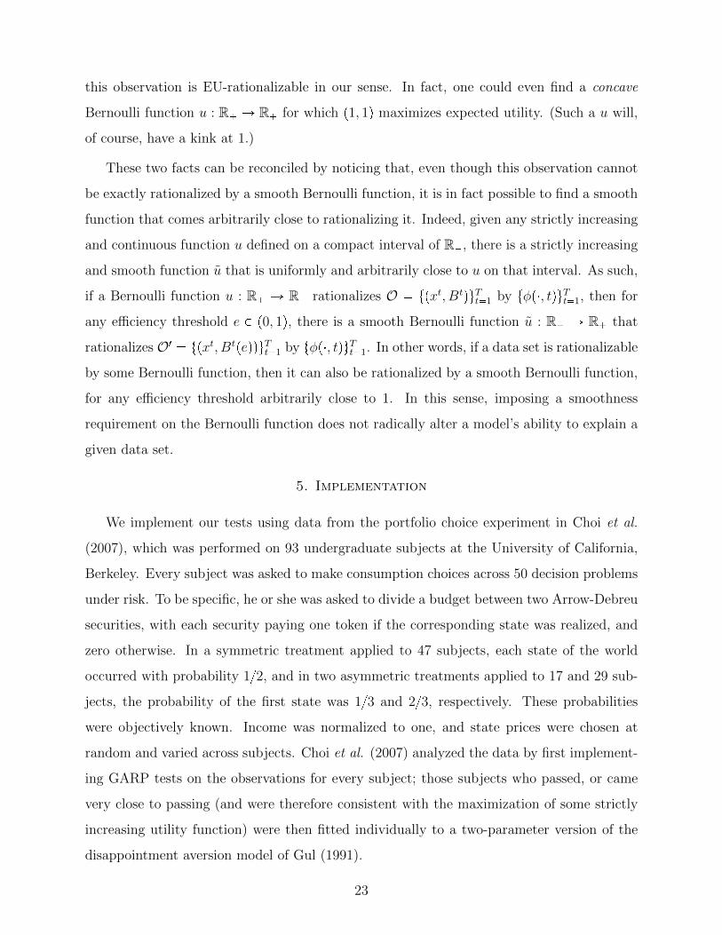
5. Implementation

We implement our tests using data from the portfolio choice experiment in Choi et al.

(2007), which was performed on 93 undergraduate subjects at the University of California,

Berkeley. Every subject was asked to make consumption choices across 50 decision problems

under risk. To be specific, he or she was asked to divide a budget between two Arrow-Debreu

securities, with each security paying one token if the corresponding state was realized, and

zero otherwise. In a symmetric treatment applied to 47 subjects, each state of the world

occurred with probability 1{2, and in two asymmetric treatments applied to 17 and 29 sub-

jects, the probability of the first state was 1{3 and 2{3, respectively. These probabilities

were objectively known. Income was normalized to one, and state prices were chosen at

random and varied across subjects. Choi et al. (2007) analyzed the data by first implement-

ing GARP tests on the observations for every subject; those subjects who passed, or came

very close to passing (and were therefore consistent with the maximization of some strictly

increasing utility function) were then fitted individually to a two-parameter version of the

disappointment aversion model of Gul (1991).

23

5.1 GARP, FGARP, DA, and EU tests

Our principal objective is to assess how the data collected by Choi et al. (2007) perform

against the nonparametric tests for DA- and EU-rationalizability that we have developed in

this paper. We can check for EU-rationalizability using the test described in Section 2, which

simply involves ascertaining whether or not there is a solution to a set of linear inequalities.

As for DA-rationalizability, recall that the disappointment aversion model is a special case of

the rank dependent utility model when there are two states; as we explained in Section 3.1,

the test for DA-rationalizability is simply a linear test after conditioning on β (and hence

the distorted probability of the favorable state, γpπHq (see (19))). We implement this test by

letting γpπHq take up to 99 different values on p0, 1q and then performing the corresponding

linear test. For example, in the symmetric case, γpπHq take on values 0.01, 0.02, . . . , 0.98,

0.99. Disappointment aversion is captured by γpπHq   1{2 (so β ¡ 0), while elation seeking

behavior is captured by γpπHq ¡ 1{2 (so β   0).

It would be natural, before testing whether a subject satisfies EU- or DA-rationalizability,

to take a few a steps back and ask a more fundamental question: is the subject’s observed

choice behavior consistent with the maximization of any well-behaved utility function? This

can be answered by checking if the observations obey the generalized axiom of revealed pref-

erence (GARP), which is necessary and sufficient for rationalizability by some continuous

and strictly increasing utility function; when a subject passes this test, we say that his or her

behavior is consistent with the increasing utility model. The GARP test was carried out by

Choi et al. (2007) and we repeat it here for all subjects. Given that we are in a contingent

consumption context, it would also be natural to ask if a subject’s behavior is rationalizable

by a continuous utility function U : Rs� Ñ R with the stronger property of stochastic mono-

tonicity (SCM); by this we mean that Upxq ¡ Upyq whenever the contingent consumption

plan x first order stochastically dominates y (where stochastic dominance is calculated with

respect to the probabilities attached to each state). A test for rationalizability by continuous

utility functions with this stronger property was recently developed by Nishimura, Ok, and

Quah (2015) and has hitherto never been implemented. A subject who passes this test is

said to be consistent with the SCM utility model.

In the experiment by Choi et al. (2007), the consumption space is R2�. When π1 �

24

π2 � 1{2, it is straightforward to check that a utility function U is stochastically monotone

if and only if it is increasing in both dimensions and symmetric. When π1 ¡ π2, then U

is stochastically monotone if and only if U is increasing in both dimensions and Upa, bq ¡

Upb, aq whenever a ¡ b. Data sets rationalizable by a utility function with this stronger

property can be characterized by a stronger version of GARP, which we shall call FGARP

(where ‘F’ stands for first order stochastic dominance).

To describe FGARP, it is useful to first recall GARP. Let D � txt : t � 1, 2, . . . , T u; in

other words, D consists of those bundles that have been observed somewhere in the data set.

We say that xt is directly revealed preferred to xt1

(for xt and xt1

in D) if pt � xt ¥ pt � xt1

, or

in other words, if xt1

P Bt, where Bt is given by (3). This defines a reflexive binary relation

on D; we call the transitive closure of this relation the revealed preference relation and say

that xt is revealed preferred to xt1

if xt is related to xt1

by the revealed preference relation.

Lastly, the bundle xt is said to be directly revealed strictly preferred to xt1

if pt � xt ¡ pt � xt1

,

or in other words, xt1

P BtzBBt, where BBt is the upper boundary of Bt. The data set O

obeys GARP if, whenever xt is revealed preferred to xt1

for any two bundles xt and xt1

in D,

then xt1

is not directly revealed strictly preferred to xt.

FGARP is a stronger version of GARP. Its general formulation can be found in Nishimura,

Ok, and Quah (2015); we shall confine our explanation of FGARP to the two special cases

relevant to our implementation. First, suppose that π1 � π2. In this case, we say that xt

is directly revealed preferred to xt1

if xt1

P Bt or xt1

P Bt, where xt1

1 � xt1

2 and xt1

2 � xt1

1 .

(Note that while we are using the same term, the concept here is weaker than the one in

the formulation of (standard) GARP.) We say that xt is revealed preferred to xt1

if they are

related by transitive closure. We say that xt is directly revealed strictly preferred to xt1

if

xt1

P BtzBBt or xt1

P BtzBBt. A data set O obeys FGARP if, for any xt and xt1

in D such

that xt is revealed preferred to xt1

, then xt1

is not directly revealed strictly preferred to xt.

It is straightforward to check that if a subject is maximizing some SCM utility function U ,

then Upxtq ¥ Upxt1

q whenever xt is revealed preferred to xt1

, and Upxtq ¡ Upxt1

q whenever xt

is directly revealed strictly preferred to xt1

; from this it follows immediately that FGARP is

a necessary property on O. It turns out that this property is also sufficient to guarantee the

rationalizability of the data by some continuous and SCM utility function (see Nishimura,

25

Ok, and Quah (2015)).

In the case where π1 ¡ π2, we say that xt is directly revealed preferred to xt1

if (i) xt1

P Bt

or (ii) xt1

P Bt and xt1

2 ¡ xt1

1 . As usual, we say that xt is revealed preferred to xt1

if they are

related via the transitive closure. We say that xt is directly revealed strictly preferred to xt1

if (i) xt1

P BtzBBt or (ii) xt1

P Bt and xt1

2 ¡ xt1

1 . The data set obeys FGARP if whenever

xt is revealed preferred to xt1

, then xt1

is not directly revealed strictly preferred to xt. Once

again, FGARP is necessary and sufficient for the rationalizability of the data set by some

continuous and SCM utility function.

To illustrate how FGARP works and to highlight its difference from GARP, suppose that

π1 � π2 � 1{2 and consider a data set with just one observation, where the bundle p1, 2q

is purchased at the prices p3, 4q. Given that there is just one observation, this data set

will obviously obey GARP. However, it is clearly not compatible with a subject maximizing

an SCM utility function, since the agent is buying more of the more expensive good, even

though both states are equiprobable. This singleton data set violates FGARP. First, (1,2) is

directly revealed preferred to itself. On the other hand, p3, 4q � p1, 2q ¡ p3, 4q � p2, 1q so p1, 2q

is also directly revealed strictly preferred to itself.

In cases where a data set O fails GARP (or FGARP), we may wish to find the efficiency

level at which it is rationalizable by a continuous and strictly increasing (stochastically

monotone) utility function. This can be done by a simple modification of GARP (FGARP).

For example, to check whether the data set is rationalizable at an efficiency threshold of

0.9, we need only modify the revealed preference and revealed strict preference relations by

replacing Bt and its upper boundary BBt with Btp0.9q (as defined by (31)) and its upper

boundary BpBtp0.9qq. A data set O then obeys GARP (FGARP) if, whenever xt is revealed

preferred to xt1

for any two bundles xt and xt1

in D, then xt1

is not directly revealed strictly

preferred to xt.

5.2 Pass rates and goodness of fit

We first test all four models on the data and the results are displayed in Table 1. Across

50 decision problems, 16 out of 93 subjects obey GARP and are therefore consistent with

the increasing utility model; subjects in the symmetric treatment perform distinctly better

26

Treatment GARP FGARP DA EU

π1 � 1{2 12/47 (26%) 1/47 (2%) 1/47 (2%) 1/47 (2%)

π1 � 1{2 4/46 (9%) 3/46 (7%) 1/46 (2%) 1/46 (2%)

Total 16/93 (17%) 4/93 (4%) 2/93 (2%) 2/93 (2%)

Table 1: Pass rates

than those in the asymmetric treatment. Of the 16 who pass GARP, only 4 pass FGARP

and so display behavior consistent with the SCM utility model. Hardly any subjects pass

the EU test and, while the DA model is in principle more permissive than EU, it does not

fare any better on these data.

Given that we observe 50 decisions for every subject, it may not be intuitively surprising

that there are so many violations of GARP (let alone more stringent conditions). Following

Choi et al. (2007), we next investigate the efficiency thresholds at which subjects pass the

different tests. We first calculate the CCEI associated with the increasing utility model, for

each of the 93 subjects. This distribution is depicted in Figure 4. (Note that this figure is a

replication of Figure 4 in Choi et al. (2007).) We can see that more than 80% of subjects

have a CCEI above 0.9, and more than 90% have a CCEI above 0.8. A first glance at these

results suggests that the data are largely consistent with the increasing utility model.

To better understand whether a CCEI of 0.9 implies the relative success or failure of a

model to explain a given data set, it is useful to postulate an alternative hypothesis of some

other form of behavior against which a comparison can be made. We adopt an approach

first suggested by Bronars (1987) that simulates random uniform consumption, i.e., which

posits that consumers are choosing randomly uniformly from their budget lines. The Bronars

(1987) approach has become common practice in the revealed preference literature as a way

of assessing the ‘power’ of revealed preference tests. We follow exactly the procedure of Choi

et al. (2007) and generate a random sample of 25,000 simulated subjects, each of whom

is choosing randomly uniformly from 50 budget lines that are selected in the same random

fashion as in the experimental setting. The dashed gray line in Figure 4 corresponds to the

CCEI distribution for our simulated subjects. The experimental and simulated distributions

are starkly different. For example, while 80% of subjects have a CCEI of 0.9 or higher,

the chance of a randomly drawn sample passing GARP at an efficiency threshold of 0.9 is

27

CCEI

Percentage≥

CCEI

0

0.1

0.2

0.3

0.4

0.5

0.6

0.7

0.8

0.9

1

0.4 0.5 0.6 0.7 0.8 0.9 1

Simulated GARP GARP

Figure 4: CCEI distribution for the increasing utility model

negligible, which lends support to increasing utility maximization as a model of choice among

contingent consumption bundles.

Going beyond Choi et al. (2007), we then calculate CCEIs for the FGARP, DA, and

EU tests among the 93 subjects. These distributions are shown in Figures 5a and 5b, which

correspond to the symmetric and asymmetric treatments, respectively. Since all of these

models are more stringent than the increasing utility model, one would expect their CCEIs

to be lower than for GARP, and they are. Nonetheless, at an efficiency index of 0.9, around

half of all subjects are consistent with the EU model, with the proportion distinctly higher

under the symmetric treatment. For the symmetric case, the performance for EU, DA, and

FGARP are very close; in fact, the CCEI distributions for DA and FGARP are almost

indistinguishable. For the asymmetric case, the performances of the different models are

more distinct: FGARP does considerably better than EU or DA and its CCEI distribution

is close to that for GARP. This is not altogether surprising and reflects the fact that FGARP

is effectively a more stringent test in the symmetric case than in the asymmetric case (see

Section 5.1). We have not depicted the CCEI distributions for the randomly generated

28

CCEI

Percentage≥

CCEI

0

0.1

0.2

0.3

0.4

0.5

0.6

0.7

0.8

0.9

1

0.4 0.5 0.6 0.7 0.8 0.9 1

Simulated GARP EU DA FGARP GARP

(a) π1 � 1{2

CCEI

Percentage≥

CCEI

0

0.1

0.2

0.3

0.4

0.5

0.6

0.7

0.8

0.9

1

0.4 0.5 0.6 0.7 0.8 0.9 1

Simulated GARP EU DA FGARP GARP

(b) π1 � 1{2

Figure 5: CCEI distributions for different models

29

data (under FGARP, DA, or EU), but plainly they will be even lower than that for GARP

and therefore very different from the CCEI distributions for the experimental subjects. We

conclude that a large proportion of the subjects behave in a way that is nearly consistent with

the EU or DA models, a group which is too sizable to be dismissed as occurring naturally

in random behavior.

5.3 Predictive success

While these results are highly suggestive, we would like a more formal way of comparing

across different candidate models of behavior. The four models being compared are, in

increasing order of stringency, increasing utility, SCM utility, disappointment aversion, and

expected utility. What is needed in comparing these models is a way of trading off a model’s

frequency of correct predictions (which favors increasing utility) with the precision of its

predictions (which favors expected utility). To do this, we make use of an axiomatic measure

of predictive success proposed by Selten (1991). Selten’s index of predictive success (which

we shall refer to simply as the Selten index) is defined as the difference between the relative

frequency of correct predictions (the ‘hit rate’) and the relative size of the set of predicted

outcomes (the ‘precision’). Our use of this index to evaluate different consumption models

is not novel; see, in particular, Beatty and Crawford (2011).

To calculate the Selten index, we need the empirical frequency of correct predictions

and the relative size of the set of predicted outcomes. To measure the latter, we use the

frequency of hitting the set of predicted outcomes with uniform random draws. Specifically,

for each subject, we generate 1,000 synthetic data sets containing consumption bundles

chosen randomly uniformly from the actual budget sets facing that subject. (Recall that

each subject in Choi et al. (2007) faced a different collection of 50 budget sets.) For a given

efficiency threshold and for each model, we calculate the Selten index for every subject, which

is either 1 (pass) or 0 (fail) minus the fraction of the 1,000 randomly simulated subject-specific

data sets that pass the test (for that model).18 The index ranges from �1 to 1, where �1

18 Each of the 1,000 synthetic data sets is subjected to a test of GARP, FGARP, DA, and EU. We test for

GARP and FGARP using Warshall’s algorithm and the EU test is linear, so these tests are computationally

undemanding. The test for DA-rationalizability is more computationally intensive, since each test involves

performing 99 linear tests (see the earlier discussion in this section).

30

Efficiency Level

0.80 0.85 0.90 0.95 1.00G

AR

Pπ1 � 1{2

42/47 (89%) 40/47 (85%) 38/47 (81%) 32/47 (68%) 12/47 (26%)

0.83 [0.94] 0.84 [0.99] 0.81 [1.00] 0.68 [1.00] 0.26 [1.00]

π1 � 1{243/46 (93%) 40/46 (87%) 37/46 (80%) 29/46 (63%) 4/46 (9%)

0.88 [0.94] 0.86 [0.99] 0.80 [1.00] 0.63 [1.00] 0.09 [1.00]

Total85/93 (91%) 80/93 (86%) 75/93 (81%) 61/93 (66%) 16/93 (17%)

0.86 [0.94] 0.85 [0.99] 0.81 [1.00] 0.66 [1.00] 0.17 [1.00]

FG

AR

P

π1 � 1{237/47 (79%) 36/47 (77%) 30/47 (64%) 23/47 (49%) 1/47 (2%)

0.79 [1.00] 0.77 [1.00] 0.64 [1.00] 0.49 [1.00] 0.02 [1.00]

π1 � 1{241/46 (89%) 36/46 (78%) 33/46 (72%) 26/46 (57%) 3/46 (7%)

0.88 [0.99] 0.78 [1.00] 0.72 [1.00] 0.57 [1.00] 0.07 [1.00]

Total78/93 (84%) 72/93 (77%) 63/93 (68%) 49/93 (53%) 4/93 (4%)

0.83 [0.99] 0.77 [1.00] 0.68 [1.00] 0.53 [1.00] 0.04 [1.00]

DA

π1 � 1{237/47 (79%) 36/47 (77%) 30/47 (64%) 23/47 (49%) 1/47 (2%)

0.78 [1.00] 0.77 [1.00] 0.64 [1.00] 0.49 [1.00] 0.02 [1.00]

π1 � 1{237/46 (80%) 31/46 (67%) 20/46 (43%) 12/46 (26%) 1/46 (2%)

0.80 [1.00] 0.67 [1.00] 0.43 [1.00] 0.26 [1.00] 0.02 [1.00]

Total74/93 (80%) 67/93 (72%) 50/93 (54%) 35/93 (38%) 2/93 (2%)

0.79 [1.00] 0.72 [1.00] 0.54 [1.00] 0.38 [1.00] 0.02 [1.00]

EU

π1 � 1{237/47 (79%) 36/47 (77%) 30/47 (64%) 18/47 (38%) 1/47 (2%)

0.79 [1.00] 0.77 [1.00] 0.64 [1.00] 0.38 [1.00] 0.02 [1.00]

π1 � 1{231/46 (67%) 28/46 (61%) 18/46 (39%) 12/46 (26%) 1/46 (2%)

0.67 [1.00] 0.61 [1.00] 0.39 [1.00] 0.26 [1.00] 0.02 [1.00]

Total68/93 (73%) 64/93 (69%) 48/93 (52%) 30/93 (32%) 2/93 (2%)

0.73 [1.00] 0.69 [1.00] 0.52 [1.00] 0.32 [1.00] 0.02 [1.00]

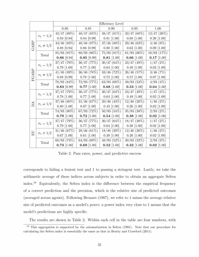
Table 2: Pass rates, power, and predictive success

corresponds to failing a lenient test and 1 to passing a stringent test. Lastly, we take the

arithmetic average of these indices across subjects in order to obtain an aggregate Selten

index.19 Equivalently, the Selten index is the difference between the empirical frequency

of a correct prediction and the precision, which is the relative size of predicted outcomes

(averaged across agents). Following Bronars (1987), we refer to 1 minus the average relative

size of predicted outcomes as a model’s power; a power index very close to 1 means that the

model’s predictions are highly specific.

The results are shown in Table 2. Within each cell in the table are four numbers, with

19 This aggregation is supported by the axiomatization in Selten (1991). Note that our procedure for

calculating the Selten index is essentially the same as that in Beatty and Crawford (2011).

31

the pass rate in the top row and, in the lower row, the Selten index and the power, with

the latter in brackets. For example, with π1 � 1{2 and at an efficiency threshold of 0.8,

42 out of 47 subjects (89%) pass GARP, the power is 0.94, and so the Selten index is

0.83 � 0.89 � p1 � 0.94q. What emerges immediately is that, at any efficiency level and

for any model, the Selten indices of predictive success are almost completely determined by

the pass rates. This is because all of the models have uniformly high power (in fact, very

close to 1). It turns out that with 50 observations for each subject, even the increasing

utility model has very high power. Given this, the Selten index ranks the increasing utility

model as the best, followed by SCM utility, disappointment aversion, and expected utility; this

ranking holds at any efficiency level and across both treatments. All four models have indices

well within the positive range, indicating that they are clearly superior to the hypothesis

of uniform random choice (which has a Selten index of 0). While academic discussion is

often focussed on comparing different models that have been tailor-made for decisions under

risk and uncertainty, these findings suggest that we should not take it for granted that such

models are necessarily better than the standard increasing utility model. At least in the

data analyzed here, one could argue that this model does a better job in explaining the data,

even after accounting for its relative lack of specificity.

5.4 Conditional predictive success

Our next objective is to investigate the success of the EU and DA models in explaining

agent behavior, conditional on the agent maximizing some utility function. To do this,

we first identify, at a given efficiency threshold, those subjects who pass GARP at that

threshold. For each of these subjects, we then generate 1,000 synthetic data sets that obey

GARP at the same efficiency threshold and are thus consistent with the increasing utility

model.20 (Note that since we focus on five different efficiency thresholds, this implies that we

20 The procedure for creating a synthetic data set is as follows. We randomly select a budget line (out

of the 50 budget lines) and then randomly choose a bundle on that line. We next randomly select a second

budget line, and then randomly choose from that part of the line which guarantees that this observation,

along with the first, obeys GARP (or, in the case where the efficiency index is lower than 1, a modified

version of GARP). We then randomly select a third budget line, and choose a random bundle on that part

of the line which guarantees that the three observations together obey GARP (or modified GARP). Note

that there must exist such a bundle on the third budget line; indeed it can be chosen to be the demand (on

the third budget line) of any utility function rationalizing the first two observations. We then select a fourth

budget line, and so on.

32

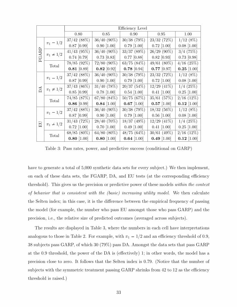
Efficiency Level

0.80 0.85 0.90 0.95 1.00

FG

AR

Pπ1 � 1{2

37/42 (88%) 36/40 (90%) 30/38 (79%) 23/32 (72%) 1/12 (8%)

0.87 [0.99] 0.90 [1.00] 0.79 [1.00] 0.72 [1.00] 0.08 [1.00]

π1 � 1{241/43 (95%) 36/40 (90%) 33/37 (89%) 26/29 (90%) 3/4 (75%)

0.74 [0.79] 0.73 [0.83] 0.77 [0.88] 0.82 [0.93] 0.73 [0.98]

Total78/85 (92%) 72/80 (90%) 63/75 (84%) 49/61 (80%) 4/16 (25%)

0.81 [0.89] 0.82 [0.92] 0.78 [0.94] 0.77 [0.97] 0.25 [1.00]

DA

π1 � 1{237/42 (88%) 36/40 (90%) 30/38 (79%) 23/32 (72%) 1/12 (8%)

0.87 [0.99] 0.90 [1.00] 0.79 [1.00] 0.72 [1.00] 0.08 [1.00]

π1 � 1{237/43 (86%) 31/40 (78%) 20/37 (54%) 12/29 (41%) 1/4 (25%)

0.85 [0.99] 0.78 [1.00] 0.54 [1.00] 0.41 [1.00] 0.25 [1.00]

Total74/85 (87%) 67/80 (84%) 50/75 (67%) 35/61 (57%) 2/16 (12%)

0.86 [0.99] 0.84 [1.00] 0.67 [1.00] 0.57 [1.00] 0.12 [1.00]

EU

π1 � 1{237/42 (88%) 36/40 (90%) 30/38 (79%) 18/32 (56%) 1/12 (8%)

0.87 [0.99] 0.90 [1.00] 0.79 [1.00] 0.56 [1.00] 0.08 [1.00]

π1 � 1{231/43 (72%) 28/40 (70%) 18/37 (49%) 12/29 (41%) 1/4 (25%)

0.72 [1.00] 0.70 [1.00] 0.49 [1.00] 0.41 [1.00] 0.25 [1.00]

Total68/85 (80%) 64/80 (80%) 48/75 (64%) 30/61 (49%) 2/16 (12%)

0.80 [1.00] 0.80 [1.00] 0.64 [1.00] 0.49 [1.00] 0.12 [1.00]

Table 3: Pass rates, power, and predictive success (conditional on GARP)

have to generate a total of 5,000 synthetic data sets for every subject.) We then implement,

on each of these data sets, the FGARP, DA, and EU tests (at the corresponding efficiency

threshold). This gives us the precision or predictive power of these models within the context

of behavior that is consistent with the (basic) increasing utility model. We then calculate

the Selten index; in this case, it is the difference between the empirical frequency of passing

the model (for example, the number who pass EU amongst those who pass GARP) and the

precision, i.e., the relative size of predicted outcomes (averaged across subjects).

The results are displayed in Table 3, where the numbers in each cell have interpretations

analogous to those in Table 2. For example, with π1 � 1{2 and an efficiency threshold of 0.9,

38 subjects pass GARP, of which 30 (79%) pass DA. Amongst the data sets that pass GARP

at the 0.9 threshold, the power of the DA is (effectively) 1; in other words, the model has a

precision close to zero. It follows that the Selten index is 0.79. (Notice that the number of

subjects with the symmetric treatment passing GARP shrinks from 42 to 12 as the efficiency

threshold is raised.)

33

Efficiency Level

0.80 0.85 0.90 0.95 1.00D

A

π1 � 1{237/37 (100%) 36/36 (100%) 30/30 (100%) 23/23 (100%) 1/1 (100%)

0.11 [0.11] 0.29 [0.29] 0.65 [0.65] 0.97 [0.97] 1.00 [1.00]

π1 � 1{237/41 (90%) 31/36 (86%) 20/33 (61%) 12/26 (46%) 1/3 (33%)

0.89 [0.99] 0.86 [1.00] 0.61 [1.00] 0.46 [1.00] 0.33 [1.00]

Total74/78 (95%) 67/72 (93%) 50/63 (79%) 35/49 (71%) 2/4 (50%)

0.52 [0.57] 0.57 [0.64] 0.63 [0.83] 0.70 [0.99] 0.50 [1.00]

EU

π1 � 1{237/37 (100%) 36/36 (100%) 30/30 (100%) 18/23 (78%) 1/1 (100%)

0.23 [0.23] 0.50 [0.50] 0.81 [0.81] 0.77 [0.99] 1.00 [1.00]

π1 � 1{231/41 (76%) 28/36 (78%) 18/33 (55%) 12/26 (46%) 1/3 (33%)

0.76 [1.00] 0.78 [1.00] 0.55 [1.00] 0.46 [1.00] 0.33 [1.00]

Total68/78 (87%) 64/72 (89%) 48/63 (76%) 30/49 (61%) 2/4 (50%)

0.51 [0.63] 0.64 [0.75] 0.67 [0.91] 0.61 [0.99] 0.50 [1.00]

Table 4: Pass rates, power, and predictive success (conditional on FGARP)

Perhaps the first feature worth highlighting in this table is that the EU and DA models

remain very precise, with power indices that are very close to 1. In other words, even if we are

choosing randomly amongst data sets that obey GARP, the probability of choosing a data

set obeying EU or DA is close to zero. Nonetheless, the DA and EU models do in fact capture

a large proportion of those subjects who display utility-maximizing behavior. Since both DA

and EU models are almost equally precise, the Selten index favors the DA model and this

is true at all efficiency thresholds. Closer examination suggests that the main difference in

performance between the two models arises from the asymmetric treatment, where DA is

better at explaining the subjects’ behavior.

Under the symmetric treatment, the performance of the SCM utility model is also very

similar to that for EU and DA. But for the case of asymmetric treatment, there is an

interesting departure: while the pass rate for FGARP is significantly higher than that for

DA, the power is also significantly lower. This leads to the DA model having a higher Selten

index at the 0.8 and 0.85 efficiency thresholds, while the SCM utility model performs better

at higher efficiency levels.

An interesting question left largely unanswered by Table 3 is the precision of the DA

or EU models, relative to the SCM utility model. Put another way, does the DA model

impose significantly greater restrictions on the data, beyond that imposed by an SCM utility

34

function? To examine this issue systematically, we build a table similar to Table 3 except

that now we confine our attention to those subjects who pass FGARP (rather than GARP)

at a given threshold. For each of these subjects, we then generate 1,000 synthetic data sets

that obey FGARP at that threshold and are thus consistent with the SCM utility model

(using a procedure analogous to that used for generating random data sets obeying GARP).

We then implement the EU and DA tests on these data sets. This gives us the precision of

these models relative to the SCM utility model; based on this we may then calculate Selten’s

index of predictive success.

The results are displayed in Table 4, where the numbers in each cell have interpretations

analogous to those in Table 3. Perhaps the first observation to make is that the EU and DA

models are no longer almost perfectly precise for the symmetric case. For example, at an

efficiency threshold of 0.9, the power of the DA model is 0.65; in other words, the probability

of a data set obeying the DA model, when it is drawn from data sets obeying FGARP is

roughly 0.35. The EU model is more precise but, even in that case, the power is clearly

below 1. This suggests that the symmetry of the utility function (which is essentially what

the SCM utility model requires in this case) sharply narrows the collection of permissible

data sets, so much so that the relative power of the DA model is no longer close to 1. On

the other hand, the DA model’s relative precision remains close to 1 in the asymmetric case,

where the FGARP test is significantly less stringent. The picture is mixed if we compare

the Selten indices of the DA and EU models, with the DA model performing worse at the

0.9 threshold but better at 0.95. Whenever DA ranks below EU, it is driven by the relative

imprecision of the DA model in the symmetric case. Significantly, even in the symmetric

case, both models retain their predictive power, with positive Selten indices.

Appendix

The proof of Theorem 1 uses the following lemma.

Lemma 1. Let tCtuTt�1 be a finite collection of constraint sets in Rs� that are compact and

downward closed (i.e., if x P Ct then so is y P Rs� such that y   x) and let the functions

tφp�, tquTt�1 be continuous and increasing in all dimensions. Suppose that there is a finite set

X of R�, a strictly increasing function u : X Ñ R�, and tM tutPT such that the following

35

holds:

M t ¥ φpupxq, tq for all x P Ct X L and (32)

M t ¡ φpupxq, tq for all x P pCtzBCtq X L, (33)

where L � X s and upxq � pupx1q, upx2q, . . . , upxsqq. Then there is a Bernoulli function

u : R� Ñ R� that extends u such that

M t ¥ φpupxq, tq for all x P Ct and (34)

if x P Ct and M t � φpupxq, tq, then x P BCt X L and M t � φpupxq, tq. (35)

Remark: The property (35) needs some explanation. Conditions (32) and (33) allow for

the possibility that M t � φpupx1q, tq for some x1 P BCt X L; we denote the set of points in

BCt X L with this property by X 1. Clearly any extension u will preserve this property, i.e.,

M t � φpupx1q, tq for all x1 P X 1. Property (35) says that we can choose u such that for all

x P CtzX 1, we have M t ¡ φpupxq, tq.

Proof: We shall prove this result by induction on the dimension of the space containing

the constraint sets. It is trivial to check that the claim is true if s � 1. In this case, L consists

of a finite set of points on R� and each Ct is a closed interval with 0 as its minimum. Now

let us suppose that the claim holds for s � m and we shall prove it for s � m � 1. If, for

each t, there is a strictly increasing and continuous utility function ut : R� Ñ R� extending

u such that (34) and (35) hold, then the the same conditions will hold for the increasing and

continuous function u � mintPT ut. So we can focus our attention on constructing ut for a

single constraint set Ct.

Suppose X � t0, r1, r2, r3, . . . , rIu, with r0 � 0   ri   ri�1, for i � 1, 2, . . . , I � 1. Let

r � maxtr P R� : pr, 0, 0, . . . , 0q P Ctu and suppose that pri, 0, 0, . . . , 0q P Ct if and only if

i ¤ N (for some N ¤ I). Consider the collection of sets of the form Di � ty P Rm� : pri, yq P

Ctu (for i � 1, 2, . . . , N); this is a finite collection of compact and downward closed sets in

Rm� . By the induction hypothesis applied to tDiuNi�1, with tφpupriq, �, tquNi�1 as the collection

of functions, there is a strictly increasing function u� : R� Ñ R� extending u such that

M t ¥ φpupriq,u�pyq, tq for all pri, yq P Ct and (36)

36

if pri, yq P Ct and M t � φpupriq,u�pyq, tq, then pri, yq P BCt X L and M t � φpupri, yq, tq.

(37)

For each r P r0, rs, define

Uprq � tu ¤ u�prq : maxtφpu,u�pyq, tq : pr, yq P Ctu ¤M tu.

This set is nonempty; indeed uprkq � u�prkq P Uprq, where rk is the largest element in

X that is weakly smaller than r. This is because, if pr, yq P Ct then so is prk, yq, and (36)

guarantees that φpuprkq,u�pyq, tq ¤M t. The downward closedness of Ct and the fact that u�

is increasing also guarantees that Uprq � Upr1q whenever r   r1. Now define uprq � supUprq;

the function u has a number of significant properties. (i) For r P X , uprq � u�prq � uprq (by

the induction hypothesis). (ii) u is a nondecreasing function since U is nondecreasing. (iii)

uprq ¡ uprkq if r ¡ rk, where rk is largest element in X smaller than r. Indeed, because Ct is

compact and φ continuous, φpuprq,u�pyq, tq ¤M t for all pr, yq P Ct. By way of contradiction,

suppose uprq � uprkq and hence uprq   u�prq. It follows from the definition of uprq that, for

any sequence un, with uprq   un   u�prq and limnÑ8 un � uprq, there is pr, ynq P Ct such

that φpun,u�pynq, tq ¡ M t. Since Ct is compact, we may assume with no loss of generality

that yn Ñ y and pr, yq P Ct, from which we obtain φpuprq,u�pyq, tq � M t. Since Ct is

downward closed, prk, yq P Ct and, since uprkq � u�prkq, we have φpu�prk, yq, tq � M t. This

can only occur if prk, yq P BCt X L (because of (37)), but it is clear that prk, yq R BCt since

prk, yq   pr, yq. (iv) If rn   ri for all n and rn Ñ ri P X , then uprnq Ñ u�priq. Suppose to

the contrary, that the limit is u   u�priq � upriq. Since u� is continuous, we can assume,

without loss of generality, that uprnq   u�prnq. By the compactness of Ct, the continuity

of φ, and the definition of u, there is prn, ynq P Ct such that φpuprnq,u

�pynq, tq � M t. This

leads to φpu,u�py1q, tq � M t, where y1 is an accumulation point of yn and pri, y1q P Ct. But

since φ is strictly increasing, we obtain φpu�priq,u�py1q, tq ¡M t, which contradicts (36).

Given the properties of u, we can find a continuous and strictly increasing function ut

such that ut extends u, i.e., utprq � uprq for r P X , utprq   u�prq for all r P R�zX and

utprq   uprq ¤ u�prq for all r P r0, rszX . (In fact we can choose ut to be smooth everywhere

except possibly on X .) We claim that (34) and (35) are satisfied for Ct. To see this, note

that for r P X and pr, yq P Ct, the induction hypothesis guarantees that (36) and (37) hold

and they will continue to hold if u� is replaced by ut. In the case where r R X and pr, yq P Ct,

37

since utprq   uprq and φ is increasing, we obtain M t ¡ φputpr, yq, tq. QED

Proof of Theorem 1: This follows immediately from Lemma 1 if we set Ct � Bt, and

M t � φpupxtq, tq. If u obeys conditions (8) and (9) then it obeys conditions (32) and (33).

The rationalizability of O by tφp�, tqutPT then follows from (34). QED

Proof of Proposition 1: Suppose that O is rationalizable by φ as defined by (23). For

any x in the finite lattice L, let πpxq be an element in arg minπPΠ π � upxq and let u be the

restriction of u to X . Then it is clear that the conditions (24) – (26) hold.

Conversely, suppose that there is a function π and a strictly increasing function u obeying

the conditions (24) – (26). Define Π as the convex hull of tπpxq : x P Lu; Π is a nonempty

and convex subset of ∆�� and it is compact in Rs since L is finite. Suppose that there

exists x P L and π P Π such that π � upxq   πpxq � upxq. Since π is a convex combination of

elements in tπpxq : x P Lu, there must exist x1 P L such that πpx1q � upxq   πpxq � upxq, which

contradicts (26). We conclude that πpxq � upxq � minπPΠ π � upxq for all x P L. We define

φ : Rs� Ñ R by φpuq � minπPΠ π � u. Then the conditions (24) and (25) are just versions

of (8) and (9) and so Theorem 1 guarantees that there is Bernoulli function u : R� Ñ R�

extending u such that O is rationalizable by V pxq � φpupxqq. QED

Proof of Proposition 2: Suppose O is rationalizable by φ as defined by (27). Let u be the

restriction of u to X . For any x in L, let πpxq be an element in arg minπP∆��tπ �upxq�cpπqu,

and let cpxq � cpπpxqq. Then it is clear that the conditions (28) – (30) hold.

Conversely, suppose that there is a strictly increasing function u and functions π and

c obeying conditions (28) – (30). For every π P ∆��, define cpπq � maxxPLtcpxq � pπ �

πpxqq � upxqu. It follows from (30) that cpx1q ¥ cpxq � pπpx1q � πpxqq � upxq for all x P L.

Therefore, cpπpx1qq � cpx1q for any x1 P L. The function c is convex and continuous but

it need not obey the boundary condition. However, we know there is a function c defined

on ∆�� that is convex, continuous, obeys the boundary condition, with cpπq ¥ cpπq for

all π P ∆�� and cpπq � cpπq for π P tπpxq : x P Lu. We claim that, with c so defined,

minπP∆��tπ � upxq � cpπqu � πpxq � upxq � cpxq for all x P L. Indeed, for any π P ∆��,

π � upxq � cpπq ¥ π � upxq � cpπq ¥ π � upxq � cpxq � pπ � πpxqq � upxq � upxq � cpxq.

38

On the other hand, πpxq � upxq � cpπpxqq � πpxq � upxq � cpxq, which establishes the claim.

We define φ : Rs� Ñ R by (27); then (28) and (29) are just versions of (8) and (9) and so

Theorem 1 guarantees that there is a Bernoulli function u : R� Ñ R� extending u such that

O is rationalizable by V pxq � φpupxqq. QED

References

AFRIAT, S. N. (1967): “The Construction of Utility Functions from Expenditure Data,” Inter-national Economic Review, 8(1), 67–77.

AFRIAT, S. N. (1972): “Efficiency Estimation of Production Functions,” International EconomicReview, 13(3), 568–598.

AFRIAT, S. N. (1973): “On a System of Inequalities in Demand Analysis: An Extension of theClassical Method,” International Economic Review, 14(2), 460–472.

BAYER, R.-C., S. BOSE, M. POLISSON, and L. RENOU (2013): “Ambiguity Revealed”, IFSWorking Papers, W13/05.

BEATTY, T. K. M., and I. A. CRAWFORD (2011): “How Demanding Is the Revealed PreferenceApproach to Demand?,” American Economic Review, 101(6), 2782–2795.

BRONARS, S. G. (1987): “The Power of Nonparametric Tests of Preference Maximization,”Econometrica, 55(3), 693–698.

BROWN, D. J., and R. L. MATZKIN (1996): “Testable Restrictions on the Equilibrium Mani-fold,” Econometrica, 64(6), 1249–1262.

BUSSIECK, M. R., and S. VIGERSKE (2010): “MINLP solver software,” Wiley Encyclopedia ofOperations Research and Management Science.

CHAMBERS, C. P., C. LIU, and S.-K. MARTINEZ (2015): “A Test for Risk-Averse ExpectedUtility,” Mimeo.

CHAMBERS, C. P., F. ECHENIQUE, and K. SAITO (2015): “Testable Implications of Trans-lation Invariance and Homotheticity: Varational, Maxmin, CARA and CRRA Preferences,”Mimeo.

CHOI, S., R. FISMAN, D. GALE, and S. KARIV (2007): “Consistency and Heterogeneity ofIndividual Behavior under Uncertainty,” American Economic Review, 97(5), 1921–1938.

DIEWERT, W. E. (1973): “Afriat and Revealed Preference Theory,” Review of Economic Studies,40(3), 419–425.

DIEWERT, W. E. (2012): “Afriat’s Theorem and some Extensions to Choice under Uncertainty,”Economic Journal, 122(560), 305–331.

ECHENIQUE, F., and K. SAITO (2015): “Savage in the Market,” Econometrica, 83(4), 1467–1495.

39

FORGES, F., and E. MINELLI (2009): “Afriat’s Theorem for General Budget Sets,” Journal ofEconomic Theory, 144(1), 135–145.

FOSTEL, A., H. E. SCARF, and M. J. TODD (2004): “Two New Proofs of Afriat’s Theorem,”Economic Theory, 24(1), 211–219.

GILBOA, I., and D. SCHMEIDLER (1989): “Maxmin Expected Utility with Non-Unique Prior,”Journal of Mathematical Economics, 18(2), 141–153.

GREEN, R. C., and S. SRIVASTAVA (1986): “Expected Utility Maximization and DemandBehavior,” Journal of Economic Theory, 38(2), 313–323.

GUL, F. (1991): “A Theory of Disappointment Aversion,” Econometrica, 59(3), 667–686.

HALEVY, Y., D. PERSITZ, and L. ZRILL (2014): “Parametric Recoverability of Preferences,”Mimeo.

KOSZEGI, B., and M. RABIN (2007): “Reference-Dependent Risk Attitudes,” American Eco-nomic Review, 97(4), 1047–1073.

KUBLER, F., L. SELDEN, and X. WEI (2014): “Asset Demand Based Tests of Expected UtilityMaximization,” American Economic Review, 104(11), 3459–3480.

MACCHERONI, F., M. MARINACCI, and A. RUSTICHINI (2006): “Ambiguity Aversion, Ro-bustness, and the Variational Representation of Preferences,” Econometrica, 74(6), 1447–1498.

MASATLIOGLU, Y., and C. RAYMOND (2014): “A Behavioral Analysis of Stochastic ReferenceDependence,” Mimeo.

NISHIMURA, H., E. A. OK, and J. K.-H. QUAH (2015): “A Comprehensive Approach to Re-vealed Preference Theory,” Discussion Paper, Department of Economics, University of Ox-ford, 752.

QUIGGIN, J. (1982): “A Theory of Anticipated Utility”, Journal of Economic Behavior andOrganization, 3(4), 323–343.

SELTEN, R. (1991): “Properties of a Measure of Predictive Success,” Mathematical Social Sci-ences, 21(2), 153–167.

TVERSKY, A., and D. KAHNEMAN (1992): “Advances in Prospect Theory: Cumulative Rep-resentation of Uncertainty,” Journal of Risk and Uncertainty, 5(4), 297–323.

VARIAN, H. R. (1982): “The Nonparametric Approach to Demand Analysis,” Econometrica,50(4), 945–973.

VARIAN, H. R. (1983a): “Non-Parametric Tests of Consumer Behaviour,” Review of EconomicStudies, 50(1), 99–110.

VARIAN, H. R. (1983b): “Nonparametric Tests of Models of Investor Behavior,” Journal ofFinancial and Quantitative Analysis, 18(3), 269–278.

VARIAN, H. R. (1988): “Estimating Risk Aversion from Arrow-Debreu Portfolio Choice,” Econo-metrica, 56(4): 973–979.

VARIAN, H. R. (1990): “Goodness-of-Fit in Optimizing Models,” Journal of Econometrics, 46(1–2), 125–140.

40