Reversible methods of Runge-Kutta type for Index-2 DAEs

Numerische Mathematik manuscript No.(will be inserted by the editor)

Reversible methods of Runge-Kutta type forIndex-2 DAEs

R.P.K. Chan1, P. Chartier2, A. Murua3

1 Department of Mathematics, Tamaki Campus, The University of Auckland,Private Bag 92019, Auckland, NEW ZEALAND.

2 INRIA Rennes, Campus de Beaulieu, 35042 Rennes Cedex, FRANCE.3 Konputazio Zientziak eta A.A. saila, Informatika Fakultatea, EHU, Donostia,

SPAIN.

December 17, 2003

Summary A new interpretation of Runge-Kutta methods for dif-ferential algebraic equations (DAEs) of index 2 is presented, where astep of the method is described in terms of a smooth map (smoothalso with respect to the stepsize). This leads to a better understand-ing of the convergence behavior of Runge-Kutta methods that are notstiffly accurate. In particular, our new framework allows for the uni-fied study of two order-improving techniques for symmetric Runge-Kutta methods (namely post-projection and symmetric projection)specially suited for solving reversible index-2 DAEs.

AMS Classification : 65L05, 65L06

Keywords : differential algebraic equations, index 2, reversibility,Runge-Kutta methods, symmetric projection, backward analysis.

1 Introduction

The main focus of this paper is the integration of reversible index-2 differential-algebraic equations with Runge-Kutta methods. Morespecifically, we consider index-2 DAEs in semi-explicit form1

{y′ = f(y, z), f : RM+N → RM ,0 = g(y), g : RM → RN ,

(1)

1 See [HLR89] for a definition of the notion of index.

2 R.P.K. Chan et al.

where, as is usual, gy(y)fz(y, z) is assumed to be invertible in a neigh-borhood of the exact solution, and the initial values y0, z0 are assumedto be consistent, that is,

g(y0) = 0, gy(y0)f(y0, z0) = 0.

We suppose in addition that there exist isomorphisms ρ : RM → RM ,ρ2 = IM and ρ : RN → RN such that

{ρf(y, z) = −f(ρy, z),g(ρy) = ρg(y). (2)

Note that the special case, frequently arising in practice, of me-chanical systems with holonomic constraints and an Hamiltonianfunction of the form H(q, p) = 1

2pTM(q)−1p + U(q), can be put intothe form (1) and satisfy (2). The equations of motion of nonholonomicmechanics can often be put into this form as well.

The definition we give here of reversible index-2 DAEs is relatedto reversible ODEs as follows : under some minor additional assump-tions, equations (1) can be rewritten as

y′ = f(y, θ(y)), (3)z = θ(y), (4)

where θ is the smooth function implicitely defined as the solutionof gy(y)f(y, θ(y)) = 0. It is then straightforward to check that, ifcondition (2) holds, f(ρy, θ(ρy)) = −ρf(y, θ(y)). In that case, (3) isa ρ-reversible ODE system, that is,

ρ ◦ ϕt = ϕ−t ◦ ρ,

where ϕt denotes the exact y-flow of the ODE system (3).It is known [Sto88] that the numerical flow defined by the appli-

cation of a symmetric Runge-Kutta method to a ρ-reversible ODEsystem is ρ-reversible. Backward error analysis can be applied in thatcase to show that [HLW02] the numerical flow is exponentially closeto the exact flow of a ρ-reversible ODE system (which is a perturba-tion of the original one).

This suggests that symmetric Runge-Kutta schemes might be ofinterest for the numerical integration of reversible index-2 DAEs andamongst them the important class of Gauss collocation methods.Although such methods suffer from an important order reduction[HW96], it has been shown in [CCM02b] to be of local nature, sothat once the Runge-Kutta solutions have been obtained, the originalorder of convergence can be restored by performing a suitable pro-jection (post-projection) onto the manifold M = {y ∈ RM ; g(y) = 0}.

Reversible methods of Runge-Kutta type for Index-2 DAEs 3

Another possibility is to adapt to index-2 DAEs the idea of symmetricprojection proposed in [Hai00,Hai01] for ODEs.

In a unified framework, we thus present a new interpretation ofRunge-Kutta schemes with invertible matrix, where one step of themethod is interpreted in terms of a smooth map (smooth also inthe stepsize). In addition to shedding new light toward the under-standing of the convergence behavior of general Runge-Kutta meth-ods, by establishing a connection with the concept of effective orderfor ODEs [But69], it immediately allows the application of standardbackward error analysis for ODEs. Moreover, this approach greatlysimplifies the analysis of symmetrically projected Runge-Kutta meth-ods for index-2 DAEs.

In Section 2, we shall first present an overview of the main toolsused in the paper and the motivations behind them. Section 3 will in-troduce our new framework for the study of the application of Runge-Kutta methods to index-2 DAEs. The convergence analysis for thespecial case of collocation methods will be given in Section 4, whilea backward analysis will be sketched in Section 5 whose results areparticularly useful in understanding the application of Runge-Kuttamethods (in particular with post-projection) to reversible index-2DAEs. In Section 6, we will study the special case of symmetricallyprojected methods. In Section 7, we will report on some numericalexperiments aimed at illustrating the convergence results obtainedhere as well as the properties of symmetric methods, with or withoutsymmetric projection, for long-term integration.

2 Setting up the problem : main notation and motivations

As usual when solving index-2 DAEs numerically, we will assume thatgy(y)fz(y, z) is invertible in a neighborhood of the manifold M. Moreprecisely, we will suppose that there exists a bounded and connectedopen neighborhood V of M where we can define a smooth map θ,from V to RN , such that

∀ y ∈ V,∃! z = θ(y) ∈ RN , gy(y)f(y, z) = 0 anddet[gy(y)fz(y, z)] '= 0.

Eventually, we will refer to a Runge-Kutta scheme with coefficientmatrix A and weight vector b by R = (A, b). We hereafter assumethat A is invertible. The numerical flow of (1) corresponding to theRunge-Kutta scheme R = (A, b) is the map y∗ = Φh(y) defined by

y∗ = y + h(bT ⊗ IM )F (Y,Z), (5)


where the internal stage values Y , Z are implicitly defined by

Y = (e ⊗ y) + h(A ⊗ IM )F (Y,Z), (6)0 = G(Y ), (7)

where F (Y,Z) and G(Y ) are the vector-functions with componentsf(Yi, Zi) and g(Yi), i = 1, . . . , s. Here the question of whether Φh iswell defined for sufficiently small h arises. It is clear that, for h = 0,(6)-(7) has no solution if y '∈ M. This causes difficulties2 in studyingthe successive application of Φh as h → 0, especially when the methodis not stiffly accurate3, since the numerical solution

yn = Φh(yn−1), n ≥ 1 (8)

will not in general lie on the constraint manifold M even if y0 ∈ M.We will hereafter address this problem in a rigorous setting. We firstgive an overview.

We consider the standard projection4 y = PM(y) onto the mani-fold M implicitly defined as follows

y = y + fz(y, θ(y))µ, 0 = g(y),

and we denote µ = PRN (y). The pair (y, µ) ∈ M × RN is uniquelydefined for each y ∈ RM sufficiently close to M. This can be viewedas a change of variables from RM to M× RN .

The key to our approach is to rewrite the numerical flow Φh inthe new variables (y,λ). That is, denoting BN (0,α) ⊂ RN the openball of center 0 and radius α (where α is an arbitrarily fixed positivevalue), we define a new map Ψh as follows

Definition 1 The map Ψh parametrised by h ∈ R is the function

Ψh : M× BN (0,α) → M× RN

(y,λ) ,→ (y∗,λ∗) = (Ψ [1]h (y,λ),Ψ [2]

h (y,λ)),

defined by the equations

y = y − h2fz(y, θ(y))λ, (9)y∗ = Φh(y), (10)y∗ = y∗ + h2fz(y∗, θ(y∗))λ∗, g(y∗) = 0. (11)

2 It is only known [HW96] that (6)-(7) has a unique solution if g(y) = O(h2).3 See [HW96] for a discussion of stiffly accurate methods.4 As opposed to the symmetric projection discussed later on.


For each (y,λ) ∈ M × RN , Ψh(y,λ) represents a smooth curve onM× RN defined for sufficiently small h '= 0, which can be smoothlyextended to h = 0.

Eventually, it is worth mentioning that the two maps Φh and Ψh

are conjugate to each other in the sense that the following diagramcommutes :

Φh

y ,−→ y∗

P ↓ ↓ P(y,λ) ,−→ (y∗,λ∗)

Ψh

(12)

As a result, the application of n steps with constant step-size h ofthe map Ψh, starting from a point (y, 0) with y on the manifold M,may be seen as the application of n steps of the Runge-Kutta methodΦh with a final projection step. This is exactly what we called post-projection in [CCM02b].

3 Smoothness of Ψh

The main result of this section is the following theorem :

Theorem 1 Consider a Runge-Kutta method R = (A, b) with in-vertible matrix A. There exists h > 0 such that, for any |h| < h,Ψh is well-defined and smooth on M × BN (0,α). More precisely,when considered as a function of (y,λ, h), Ψh is smooth on U :=M × BN (0,α) × (−h, h). Moreover, we have for (y∗,λ∗) = Ψh(y,λ)the estimates

∂y∗

∂λ= O(h3) and

∂λ∗

∂λ= R(∞)IN + O(h), (13)

where R(∞) = 1 − bT A−1e.

Proof According to the definitions of Φh and Ψh, (y∗,λ∗) is given bythe equations

y = y − h2fz(y, θ(y))λ, (14)Y = (e ⊗ y) + h(A ⊗ IM )F (Y , Z), (15)0 = G(Y ), (16)

y∗ = y + h(bT ⊗ IM )F (Y , Z), (17)y∗ = y∗ + h2fz(y∗, θ(y∗))λ∗, (18)0 = g(y∗). (19)


Rescaling equations (16) and (19) and using the Implicit FunctionTheorem, it is standard5 to show that, for (y,λ) ∈ M×BN(0,α) andsufficiently small |h|, equations (14-15-16-17-18-19) define (y∗,λ∗) asa smooth function of (y,λ, h) with values in a neighborhood of (y, 0).The compactness of M×BN (0,α) then allows to get the same resulton the whole set U provided h is small enough.

Now, differentiating (15) and (16) with respect to λ gives succes-sively

∂Y

∂λ= −h2(e ⊗ fz) + h(A ⊗ IM )

({fy}

∂Y

∂λ+ {fz}

∂Z

∂λ

),

0 = {gy}∂Y

∂λ,

where {fy}, {fz} and {gy} are block-diagonal matrices with diagonalelements fy(Yi, Zi), fz(Yi, Zi) and gy(Yi) respectively and where fz

and later on gy are evaluted at (y, θ(y)). Inserting the first equationinto the second one we obtain

0 = {gy}(A ⊗ IM ){fy}∂Y

∂λ+ {gy}(A ⊗ IM ){fz}

∂Z

∂λ− h{gy}(e ⊗ fz),

so that we get ∂Z∂λ = O(h) and ∂Y

∂λ = O(h2). Eventually, previousequation becomes

0 = {gy}(A ⊗ IM ){fz}∂Z

∂λ− h{gy}(e ⊗ fz) + O(h2),

and we easily get

∂Z

∂λ= h({gy}(A ⊗ IM ){fz})−1{gy}(e ⊗ fz) + O(h2),

= h(A−1e ⊗ IN ) + O(h2), (20)

and

∂Y

∂λ= −h2(e ⊗ fz) + h(A ⊗ IM )(Is ⊗ fz + O(h))

∂Z

∂λ+ O(h3),

= −h2(e ⊗ fz) + h2 (A ⊗ fz)(A−1e ⊗ IN ) + O(h3),= O(h3). (21)

5 See for instance Theorem 4.1 of [HW96]. The interested reader can find acomplete proof in [CCM02a]


Now, we have that y∗ = y +O(h), and taking (20), (21) into account,that ∂y∗/∂λ = O(h2). Hence, we get from g(y∗) = 0 that

0 =∂

∂λg(y∗) = gy

∂y∗

∂λ+ O(h3),

∂y∗

∂λ= h2fz

(−IN +

∂λ∗

∂λ

)+ h(bT ⊗ fz)

∂Z

∂λ+ O(h3),

= h2fz

(−R(∞)IN +

∂λ∗

∂λ

)+ O(h3),

which, taking the invertibility of gyfz into account, leads to the esti-mates (13). !

Remark 1 The estimates (13) can be rewritten as

y∗ = Ψ [1]h (y,λ) = Ψ [1]

h (y, 0) + O(h3||λ||), (22)

λ∗ = Ψ [2]h (y,λ) = (R(∞) + O(h))λ + Ψ [2]

h (y, 0), (23)

where Ψh(y, 0) can now be interpreted as the composition of one stepof the Runge-Kutta method followed by a projection step.

4 Convergence

Hereafter we will denote by ϕt the t-flow of the system (3). By defi-nition of θ(y) and the flow ϕt of (3) we have that d

dtg(ϕt(y)) ≡ 0, andtherefore g(ϕt(y)) = g(y).

Lemma 1 Let us consider the map (y∗,λ∗) = Ψh(y,λ) correspondingto a given Runge-Kutta method R = (A, b).

1. If R satisfies the conditions

C(q) :s∑

j=1

ai,jck−1j =

cki

kfor k = 1, . . . , q and i = 1, . . . , s,

then

Yi − ϕci h(y) = O(hq+1 + h3||λ||),Zi − θ(ϕci h(y)) = O(hq + h||λ||). (24)

2. If in addition R satisfies the conditions

B(q + 1) :s∑

i=1

bick−1i =

1k

for k = 1, . . . , q + 1,


then

Ψ [1]h (y,λ) = ϕh(y) + O(hq+2 + h3||λ||),

Ψ [2]h (y,λ) = (R(∞) + O(h))λ + O(hq−1). (25)

Proof According to Remark 1, it is sufficient to get estimates forΨh(y, 0), i.e. for the Runge-Kutta method followed by a projectionstep. These estimates can be found for instance in Lemma 4.3. of[HLR89]. !

Theorem 2 Let us assume that the Runge-Kutta scheme R = (A, b)satisfies C(s) and B(p) with s ≤ p ≤ 2s, and has non-zero abscissas.Given (y,λ) ∈ M × BN (0,α) such that λ = O(hs−2), it holds for|h| < h that

Ψ [1]h (y,λ) = ϕh(y) + O(hp+1 + h3‖λ‖2 + hs+2‖λ‖).

Furthermore if f is linear in z, then

Ψ [1]h (y,λ) = ϕh(y) + O(hp+1).

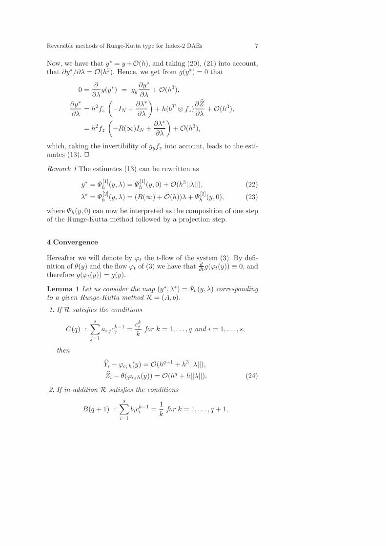
Proof Let us consider the s-degree interpolating polynomial u(t) sat-isfying u′(cih) = f(Yi, Zi), 1 ≤ i ≤ s, and u(0) = y. Since C(s)and B(p) are fulfilled with p ≥ s, the Runge-Kutta method is acollocation polynomial (see for instance the proof of Theorem II.7.8in [HNW93]), and therefore u(cih) = Yi, 1 ≤ i ≤ s, u(h) = y∗.The hypothesis λ = O(hs−2) and (24) (with q = s) imply thatYi = y(cih) + O(hs+1). From that, it follows (see for instance theproof of Theorem II.7.10 in [HNW93]) that all the derivatives ofu(t) are uniformly bounded on [0, h] as h → 0. We now consideru(t) = PM(u(t)). Clearly, u(cih) = u(cih) = Yi, u(0) = y, u(h) = y∗,and u(t) is the solution of the initial value problem

u′ = f(u, θ(u)) + δ(t), u(0) = y,

where δ(t) = u′(t) − f(u(t), θ(u(t))). Then, we can estimate y∗ −ϕh(y) = u(h)−ϕh(y) by means of the nonlinear variation-of-constantsformula (see Theorem I.14.5 of [HNW93]),

u(h) − ϕh(y) =∫ h

0R(t)δ(t)dt where R(t) =

∂

∂yϕh−t(u(t)). (26)

Since the assumption B(p) means that the quadrature formula withci as nodes and bi as weights is of order p, we arrive at

y∗ − ϕh(y) = hs∑

i=1

biR(cih)δ(cih) + O(hp+1).


y

y∗

y∗

Y4

M

u(t)

u(t)

Y1

Y2

Y3

y

Fig. 1. Polynomial u(t) and its projection u(t).

Note that, for this to be correct, we need that the derivatives of δ(t)are uniformly bounded on [0, h] as h → 0. This is a consequence ofthe uniform bounds of the derivatives of u(t) and the smoothness ofthe functions f , g, and PM.

It follows from the definition of the projection PM(y) that, fory ∈ M, we have

∂PM∂y

(y) = P (y),where P (y) = I − fz(gyfz)−1gy(y, θ(y)).

Differentiating the equality u(t) = PM(u(t)) with respect to t andevaluating at t = cih, we obtain

u′(cih) =∂PM∂y

(u(cih))u′(cih) = P (Yi)f(Yi, Zi), 1 ≤ i ≤ s. (27)

It is straightforward to check the identities P (y)f(y, θ(y)) ≡ f(y, θ(y))and P (y)fz(y, θ(y)) ≡ 0, which together with (27) imply that

δ(cih) = P (Yi)(f(Yi, Zi) − f(Yi, θ(Yi)) − fz(Yi, θ(Yi))(Zi − θ(Yi))).

This identically vanishes if f is linear in z, and is O(||Zi − θ(Yi)||2)otherwise. The required result for general f follows from applicationof Lemma 1 with q = s. !

From these local error estimates one can now derive global conver-gence results in a straigthforward way : it must be indeed emphasizedonce again that ϕt is defined as the flow of an ODE so that familiartechniques for studying ODEs apply.

Remark 2 Note that the order of Ψh can also be interpreted as theeffective order of Φh, as introduced in [But69], where the role of thefinishing procedure is played by the projection step.


5 Backward error analysis for symmetric methods

The reversibility of the numerical method is a key ingredient to back-ward analysis, so that we now investigate this question for Ψh. Toshow that Ψh is Θ-reversible with

Θ =[ρ 00 −IM

],

we prove, following [HLW02], that, on one hand, Ψh ◦ Θ = Θ ◦ Ψ−h

and on the other hand, Ψh is time-reversible or symmetric, i.e. satisfiesΨ−h = Ψ−1

h .We first state without proof the following lemma and then proceed

with establishing the two equalities for Ψh :

Lemma 2 Suppose that the differential-algebraic system (1) satisfiesthe reversibility conditions (2). Then the following equalities hold :

∀ (y, z) ∈ RM × RN , fz(ρy, z) = −ρfz(y, z),gy(ρy) ρ = ρ gy(y),

∀ y ∈ V such that ρy ∈ V, θ(ρy) = θ(y).

Theorem 3 Suppose that the differential-algebraic system (1) satis-fies the reversibility conditions (2). For any |h| ≤ h, we have

∀ (y,λ) ∈ M× BN (0,α), Ψ [1]h (ρy,−λ) = ρ(Ψ [1]

−h(y,λ)),

Ψ [2]h (ρy,−λ) = −(Ψ [2]

−h(y,λ)).

Proof Going back to the definition of Ψh, and replacing y, λ and hrespectively by ρy, −λ and −h in equation (9), we get

ρy − (−h)2fz(ρy, θ(ρy))(−λ) = ρy + h2(ρ fz(y, θ(y)))(−λ),= ρy,

where y is given by (9). Now, since Φ−h(ρy) = ρΦh(y), the valuesy∗∗ = Ψ [1]

−h(ρy,−λ) and λ∗∗ = Ψ [2]−h(ρy,−λ) are solution of the system

y∗∗ = ρy∗ + (−h)2fz(y∗∗, θ(y∗∗))λ∗∗,

0 = g(y∗∗) − g(ρy),

and must, by uniqueness, coincide with ρy∗ and −λ∗. !

Theorem 4 Suppose that the Runge-Kutta method R = (A, b) issymmetric. For any |h| < h and for all y ∈ M and all λ ∈ BN (0,α)such that Ψ [2]

h (y,λ) ∈ BN (0,α), the following equality holds :

Ψ−h(Ψh(y,λ)) = (y,λ).


Proof R being symmetric, the result follows immediately from thefact that the mapping P (see Diagram (12)) remains the same for hand −h. !

6 Symmetrically projected methods

In this section we consider the adaptation of symmetrically projectedmethods, as proposed in [Hai00,Hai01] for ODEs, to index-2 DAEs.Given a pth-order symmetric Runge-Kutta method R = (A, b), thesymmetric projection is a procedure aimed at preserving reversibilitywhile assuring at the same time that the numerical approximationlies on the manifold M. It proceeds in three steps (see Figure 2) andit is a map Sh from M to itself :

y = y − h2fz(y, θ(y))λ,y∗ = Φh(y),y∗ = y∗ − h2R(∞)fz(y∗, θ(y∗))λ, g(y∗) = 0,

(28)

where R(∞) = 1 − bT A−1e is the value of the stability function ofR at infinity. The reversibility of the procedure may be obtained as

g(y) = 0

y

y

y∗

h2f∗z λ

y∗

−h2fzλ

Φh y

−h2fzλ

yy∗

h2f∗z λ

y∗

g(y) = 0

Φh

Fig. 2. Symmetric projection with R(∞) = 1 (left) and R(∞) = −1 (right)

a by-product of the reversibility of Ψh. Equations (28) can indeed berewritten as

(y∗,λ∗) = Ψh(y,λ), (29)λ∗ = −R(∞)λ. (30)

The existence of (y∗,λ) satisfying equations (28) or equivalently (29)is a simple consequence of the smoothness of Ψh. Actually, equations(28) define for sufficiently small |h| ≤ h a one-step method Sh :

Definition 2 We define the map Sh parametrised by h

Sh : M → My ,→ y∗ = Sh(y)


by the equations

0 = R(∞)λ + Ψ [2]h (y,λ),

y∗ = Ψ [1]h (y,λ).

Theorem 5 For sufficiently small |h| ≤ h, the map Sh is smooth,also with respect to h. Moreover, it is reversible and of order p ifC(s) and B(p) are satisfied with s ≤ p ≤ 2s.

Proof We look for a zero of the function

K(λ) = R(∞)λ + Ψ [2]h (y,λ).

Since |R(∞)| = 1, it can be checked that

∂K

∂λ= R(∞)IN +

∂Ψ [2]h

∂λ,

= 2R(∞)IN + O(h),

is invertible for sufficiently small |h|. Now, for h = 0, K(0) = 0, sothat the Implicit Function Theorem locally defines the solution λ ofK(λ) = 0 as a smooth function of y and h. Provided 0 < h < his small enough, Sh can thus be smoothly extended over M for all|h| ≤ h.

In order to prove that y∗ = Sh(y) is an approximation of order pto the solution, it suffices to notice that λ = O(h). Inserted in theestimate (25), this gives λ = O(hs−1) and thus

y∗ = ϕh(y) + O(hmin(p+1,3+2(s−1)))

due to Theorem 2. !

Remark 3 The one-step method Sh being reversible and smoothly de-fined on M, a backward error analysis can be carried out just as inprevious section. The main difference is now that the correspondingmodified equation is an equation for y only, with first term f(y, θ(y)).

7 Numerical experiments

In this section, we compare the long-term behavior of post-projectionand symmetric projection for the Gauss methods. Since the two tech-niques give similar results for the pendulum problem, we present nu-merical experiments for the “double pendulum” whose equations ofmotion may be obtained from the Hamiltonian function

H(q, p) =12(p2

x1+ p2

z1) +

12(p2

x2+ p2

z2) + z1 + z2


and the two constraints

0 = x21 + z2

1 − 1, (31)0 = (x2 − x1)2 + (z2 − z1)2 − 1, (32)

where we have assumed that the two bodies have unit mass, thatthe gravitational constant is 1 and that the two rods are masslessand of length 1. In this form, the problem is of index 3 and theconstraints (31) and (32) have to be replaced by their first derivativeswith respect to time to get the index-2 formulation that we use forour numerical tests. In our tests, we have used the following initialvalues

(x1, z1, x2, z2, px1 , pz1, px2 , pz2) = (0.5,−√

0.75, 0,−2√

0.75, 0, 0, 0, 0)

corresponding to H = −3√

0.75, and a stepsize h = 0.1.Comparing the results of the two figures, we can make two main

observations :

– the Hamiltonian is much better preserved by symmetrically pro-jected methods than by post-projected methods. Symmetricallyprojected methods leaves the numerical solution on the constraintmanifold, while post-projected methods embeds a drift which be-comes dominant in the error.

– the three-stage post-projected method behaves much better thanthe two-stage method, and more generally, as additional experi-ments confirm it, methods with an odd number of stages behavebetter than methods with an even number of stages. This is ofcourse related to the value of the stability function at infinity. Al-though we do not have a definite explanation of this phenomenonat this stage, we suspect that the modified equation governing theevolution of λ is stable only for R(∞) = 1.

Acknowledgments

The authors are very grateful to one of the referees for pointing out aflaw in the numerical experiments and for his numerous suggestions.

References

[But69] J.C. Butcher. The effective order of Runge-Kutta methods. LectureNotes in Mathematics, vol. 109, pages 133–139, 1969. Conference onthe numerical solution of differential equations.


0 50 100 150 200 250 300 350 400 450 500−14

−12

−10

−8

−6

−4

−2

0

2 x 10−3 Hamiltonian of the problem

Time

H−H

0

0 100 200 300 400 500−4.5

−4

−3.5

−3

−2.5

−2

−1.5

−1

−0.5

0

0.5 x 10−9 Hamiltonian of the problem

Time

H−H

0Fig. 3. Evolution of the Hamiltonian for the 2-stage (left) and the 3-stage (right)Gauss methods with post-projection

[CCM02a] R.P.K. Chan, P. Chartier, and A. Murua. A new convergence analysisof Runge-Kutta methods for index-2 differential-algebraic equations.Technical report, INRIA, 2002.

[CCM02b] R.P.K. Chan, P. Chartier, and A. Murua. Post-projected Runge-Kuttamethods for index-2 differential-algebraic equations. Journal of AppliedNumerical Mathematics, 42:77–94, 2002.

[GSH99] O. Gonzalez, A.M. Stuart, and D.J. Higham. Qualitative properties ofmodified equations. IMA Journal of Numerical Analysis, 19:169–190,1999.

[Hai00] E. Hairer. Symmetric projection methods for differential equations onmanifold. BIT, 40(4):726–734, 2000.

[Hai01] E. Hairer. Geometric integration of ordinary differential equations onmanifold. BIT, 41:996–1007,2001.

[HLR89] E. Hairer, Ch. Lubich, and M. Roche. The Numerical Solution ofDifferential-Algebraic Systems by Runge-Kutta Methods. Springer-Verlag, 1989. Lecture Notes in Mathematics 1409.

0 100 200 300 400 500−2

0

2

4

6

8

10

12

14 x 10−9 Hamiltonian of the problem

Time

H−H

0

0 50 100 150 200 250 300 350 400 450 500−2

0

2

4

6

8

10

12

14x 10−11 Hamiltonian of the problem

Time

H−H

0

Fig. 4. Evolution of the Hamiltonian for the 2-stage (left) and 3-stage (right)symmetrically projected Gauss methods


[HLW02] E. Hairer, Chr. Lubich, and G. Wanner. Geometric Numerical Integra-tion, Structure-Preserving Algorithms for Ordinary Differential Equa-tions, volume 31 of Springer Series in Computational Mathematics.Springer-Verlag, 2002.

[HNW93] E. Hairer, S.P. Nørsett, and G. Wanner. Solving Ordinary DifferentialEquations, Nonstiff Problems. Springer-Verlag, second revised edition,1993. Volume 1.

[HW96] E. Hairer and G. Wanner. Solving Ordinary Differential Equations II,Stiff Problems and Differential-Algebraic Problems. Springer-Verlag,second revised edition, 1996. Volume 2.

[Rei97] S. Reich. On higher-order semi-explicit symplectic partitioned Runge-Kutta methods for constrained Hamiltonian systems. NumerischeMathematik, 76:231–247, 1997.

[Sto88] D. Stoffer. On reversible and canonical integration methods. TechnicalReport 88-05, ETH-Zurich, 1988.

Documents

Reversible methods of Runge-Kutta type for Index-2 DAEs