Embed Size (px)
Citation preview

Linear Dynamics, Lecture 1
Review of Hamiltonian Mechanics
Andy Wolski
University of Liverpool, and the Cockcroft Institute, Daresbury, UK.
November, 2012
Introduction
Joseph John Thomson, 1856-1940
Early accelerators were fairly straightforward.
Linear Dynamics, Lecture 1 1 Hamiltonian Mechanics

Introduction
Modern accelerators are more sophisticated.
Linear Dynamics, Lecture 1 2 Hamiltonian Mechanics
Introduction
For modern accelerators to operate properly, the beam
dynamics must be modelled and understood with very high
precision. There are many effects that are important, including
synchrotron radiation, interactions between the particles,
interactions with the residual gas in the vacuum chamber and
with the vacuum chamber itself, etc.
However, everything starts with understanding the motion of
individual particles through the fields from the magnets and the
RF cavities.
There are several possible approaches. We shall develop an
approach starting from the fundamentals of classical mechanics.
This requires more initial effort to derive the equations of
motion in a form appropriate for accelerator physics; but has
the benefit of providing a rigorous framework for modelling the
dynamics with the precision required for modern accelerators.
Linear Dynamics, Lecture 1 3 Hamiltonian Mechanics

Course Outline
Part I (Lectures 1 – 5): Dynamics of a relativistic charged
particle in the electromagnetic field of an accelerator beamline.
1. Review of Hamiltonian mechanics
2. The accelerator Hamiltonian in a straight coordinate system
3. The Hamiltonian for a relativistic particle in a general
electromagnetic field using accelerator coordinates
4. Dynamical maps for linear elements
5. Three loose ends: edge focusing; chromaticity; beam
rigidity.
Linear Dynamics, Lecture 1 4 Hamiltonian Mechanics
Course Outline
Part II (Lectures 6 – 10): Description of beam dynamics using
optical lattice functions.
6. Linear optics in periodic, uncoupled beamlines
7. Including longitudinal dynamics
8. Bunches of many particles
9. Coupled optics
10. Effects of linear imperfections
Linear Dynamics, Lecture 1 5 Hamiltonian Mechanics

Classical Mechanics
There are three alternative approaches to classical mechanics:
Newtonian, Lagrangian and Hamiltonian mechanics.
Formally, all these approaches are equivalent: they have the
same “physical content”, and any one can be derived from any
of the others.
So why prefer any one over the others?
It depends on the problem you are trying to solve; the
equations of motion for a given system may appear simpler in
one of the approaches than in the others. As we shall see, for
accelerator physics, Hamiltonian mechanics provides some great
advantages.
Linear Dynamics, Lecture 1 6 Hamiltonian Mechanics
Newtonian Mechanics
Isaac Newton, 1643-1727
The equation of motion of a particle of mass m subject to a
force F is:d
dtmx = F (x, x; t) (1)
where x is the velocity. Note that the dot over a variable
indicates the derivative with respect to time.
Linear Dynamics, Lecture 1 7 Hamiltonian Mechanics
Newtonian Mechanics: A Simple Example
Consider the case of a particle of fixed mass moving in one
degree of freedom, subject to a force F given by:
F = −mω2x (2)
The equation of motion becomes:
md
dtx = −mω2x (3)
or:
d2x
dt2= −ω2x (4)
This has solution:
x(t) = x0 sin (ωt+ φ0) (5)
where x0 and φ0 are constants determined by the initial values
of x(t) and x(t).
Linear Dynamics, Lecture 1 8 Hamiltonian Mechanics
Newtonian Mechanics
In Newtonian mechanics, the dynamics of the system are
defined by the force F, which in general is a function of
position x, velocity x and time t.
Given the function F, we derive the equations of motion, which
we must then solve to give the explicit dependence of the
position x (and the velocity x) on the independent parameter t.
“Physics” consists of writing down the form of the function F
for a given system.
Linear Dynamics, Lecture 1 9 Hamiltonian Mechanics
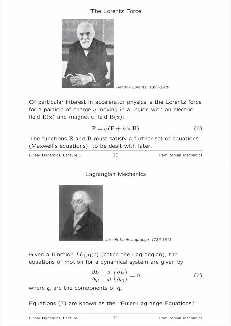
The Lorentz Force
Hendrik Lorentz, 1853-1928
Of particular interest in accelerator physics is the Lorentz force
for a particle of charge q moving in a region with an electric
field E(x) and magnetic field B(x):
F = q (E+ x×B) (6)
The functions E and B must satisfy a further set of equations
(Maxwell’s equations), to be dealt with later.
Linear Dynamics, Lecture 1 10 Hamiltonian Mechanics
Lagrangian Mechanics
Joseph-Louis Lagrange, 1736-1813
Given a function L(q, q; t) (called the Lagrangian), the
equations of motion for a dynamical system are given by:
∂L
∂qi−
d
dt
(
∂L
∂qi
)
= 0 (7)
where qi are the components of q.
Equations (7) are known as the “Euler-Lagrange Equations.”
Linear Dynamics, Lecture 1 11 Hamiltonian Mechanics

Lagrangian Mechanics: Principle of Least Action
Consider the path traced by a dynamical system on a plot of q
vs q. We can evaluate the integral S of the Lagrangian L along
the line:
S =∫ t1
t0Ldt (8)
Linear Dynamics, Lecture 1 12 Hamiltonian Mechanics
Lagrangian Mechanics: Principle of Least Action
It can be shown that the Euler-Lagrange equations (7) define a
path for which the action S is a minimum, i.e.:
δS = δ
[
∫ t1
t0Ldt
]
= 0 (9)
where the operator δ gives the change with respect to a change
in path.
Linear Dynamics, Lecture 1 13 Hamiltonian Mechanics
Lagrangian Mechanics: A Simple Example
The variables qi can be any convenient set of parameters that
describe the state of the system. The coordinates in Euclidean
space are an obvious example, (q = x) but not the only (or
necessarily best) choice.
The question is, how do we write down the function L that
contains the dynamics of the system? This question is
equivalent to “How do we write down the force F?” in
Newtonian mechanics.
It turns out that in many cases the Lagrangian is given by:
L = T − V (10)
where T is the kinetic energy of the system, and V is the
potential energy.
Linear Dynamics, Lecture 1 14 Hamiltonian Mechanics
Lagrangian Mechanics: A Simple Example
Consider a particle moving in one degree of freedom, with
kinetic energy T given by:
T =1
2mx2 (11)
and potential energy V given by:
V =1
2mω2x2 (12)
The Lagrangian is then:
L = T − V =1
2mx2 −
1
2mω2x2 (13)
Inserting the Lagrangian (13) into the Euler-Lagrange
equations (7), we find the equation of motion:
−ω2mx−d
dt(mx) = 0 (14)
or:
d2x
dt2= −ω2x (15)
Linear Dynamics, Lecture 1 15 Hamiltonian Mechanics

Lagrangian Mechanics: A Simple Example
Note that in using the Euler-Lagrange Equations to derive the
equation of motion from the Lagrangian, we treated the
coordinates x and the velocities x as independent of one
another. Of course, they are related through differentiation – x
is the rate of change of x – but for applying the
Euler-Lagrange Equations, we ignore this fact.
Lagrangian mechanics allows us to write down the equation of
motion using any convenient parameters. This sometimes
simplifies the problem compared to a treatment based on
Newtonian mechanics.
There is a third way...
Linear Dynamics, Lecture 1 16 Hamiltonian Mechanics
Hamiltonian Mechanics
William Rowan Hamilton, 1805-1865
Given a function H(x,p; t) (called the Hamiltonian), the
equations of motion for a dynamical system are given by
Hamilton’s equations:
dxi
dt=
∂H
∂pi(16)
dpi
dt= −
∂H
∂xi(17)
Linear Dynamics, Lecture 1 17 Hamiltonian Mechanics
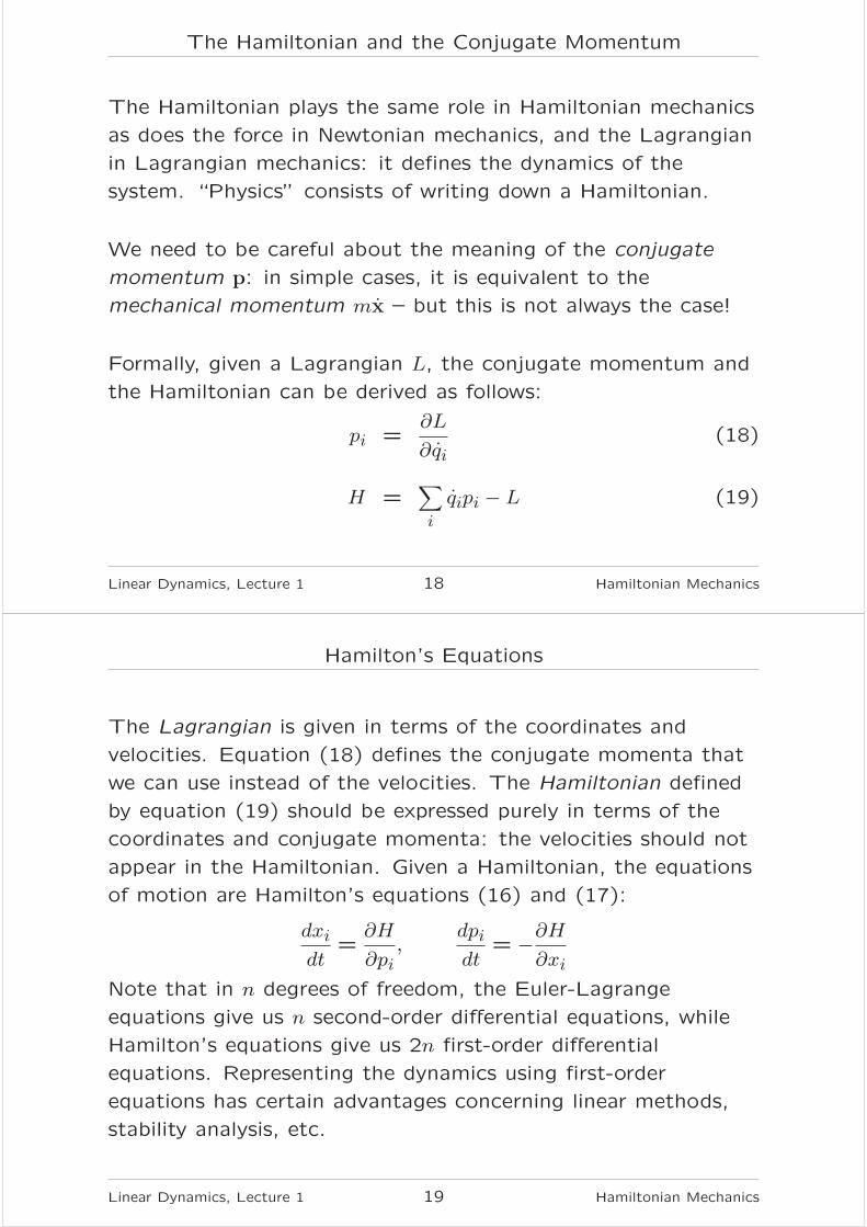
The Hamiltonian and the Conjugate Momentum
The Hamiltonian plays the same role in Hamiltonian mechanics
as does the force in Newtonian mechanics, and the Lagrangian
in Lagrangian mechanics: it defines the dynamics of the
system. “Physics” consists of writing down a Hamiltonian.
We need to be careful about the meaning of the conjugate
momentum p: in simple cases, it is equivalent to the
mechanical momentum mx – but this is not always the case!
Formally, given a Lagrangian L, the conjugate momentum and
the Hamiltonian can be derived as follows:
pi =∂L
∂qi(18)
H =∑
i
qipi − L (19)
Linear Dynamics, Lecture 1 18 Hamiltonian Mechanics
Hamilton’s Equations
The Lagrangian is given in terms of the coordinates and
velocities. Equation (18) defines the conjugate momenta that
we can use instead of the velocities. The Hamiltonian defined
by equation (19) should be expressed purely in terms of the
coordinates and conjugate momenta: the velocities should not
appear in the Hamiltonian. Given a Hamiltonian, the equations
of motion are Hamilton’s equations (16) and (17):
dxi
dt=
∂H
∂pi,
dpi
dt= −
∂H
∂xi
Note that in n degrees of freedom, the Euler-Lagrange
equations give us n second-order differential equations, while
Hamilton’s equations give us 2n first-order differential
equations. Representing the dynamics using first-order
equations has certain advantages concerning linear methods,
stability analysis, etc.
Linear Dynamics, Lecture 1 19 Hamiltonian Mechanics

Hamiltonian Mechanics: A Simple Example
Consider the Lagrangian that we looked at before:
L =1
2mx2 −
1
2mω2x2 (20)
The conjugate momentum (18) is:
px =∂L
∂x= mx (21)
Note that as usual, we treat x and x as independent of one another. Also
note that in this case, the conjugate momentum px is equal to the
mechanical momentum mx.
The Hamiltonian is:
H = xpx − L = mx2 − L (22)
or:
H =p2x
2m+
1
2mω2x2 (23)
Linear Dynamics, Lecture 1 20 Hamiltonian Mechanics
Comment: From Lagrangian to Hamiltonian Mechanics
Moving from Lagrangian to Hamiltonian mechanics essentially
involves making a change of variables from x to p. The
Hamiltonian should always be written in terms of the conjugate
momentum p rather than the velocity x.
In Lagrangian mechanics, the “state” of a system at any time
is defined by specifying values for the coordinates x (or more
generally q) and the velocity x (or q).
In Hamiltonian mechanics, the “state” of a system at any time
is defined by specifying values for the coordinates x (or more
generally q) and the momentum p.
Linear Dynamics, Lecture 1 21 Hamiltonian Mechanics
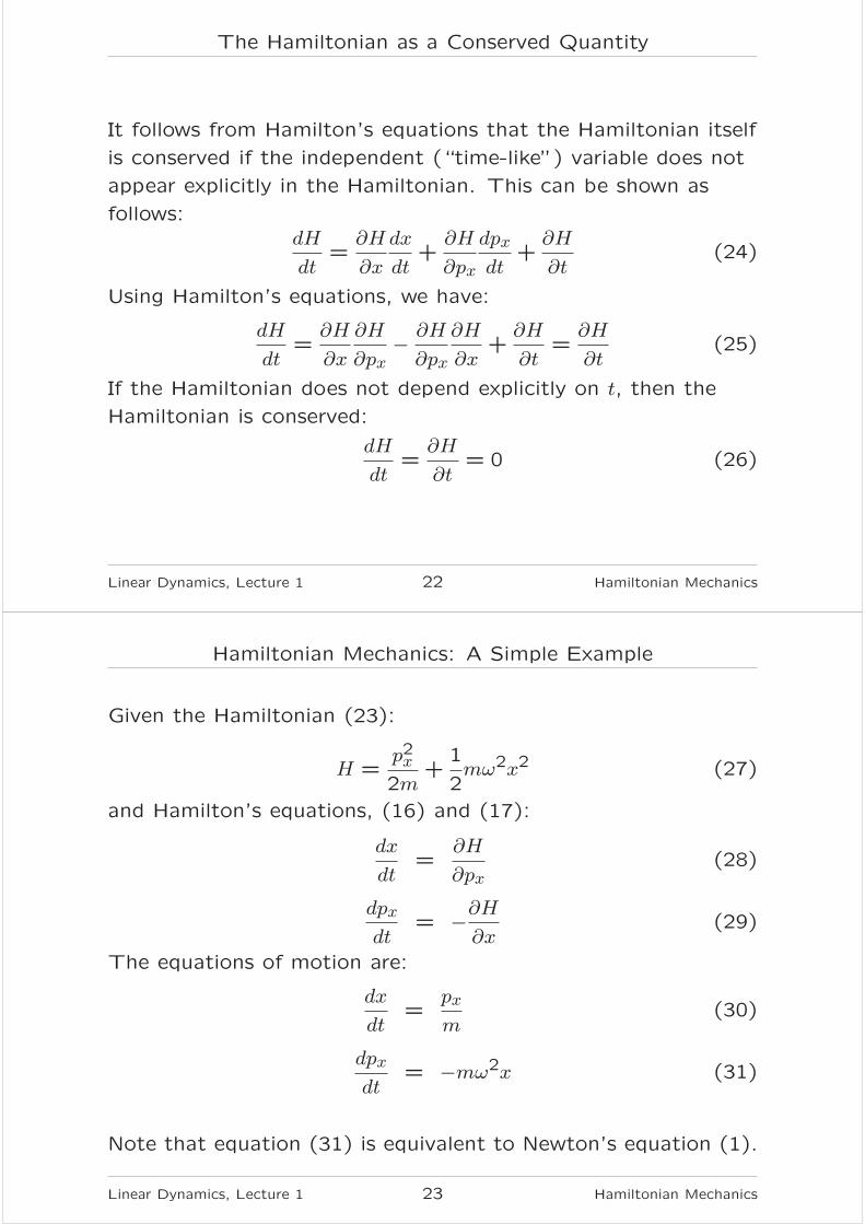
The Hamiltonian as a Conserved Quantity
It follows from Hamilton’s equations that the Hamiltonian itself
is conserved if the independent (“time-like”) variable does not
appear explicitly in the Hamiltonian. This can be shown as
follows:dH
dt=
∂H
∂x
dx
dt+
∂H
∂px
dpx
dt+
∂H
∂t(24)
Using Hamilton’s equations, we have:
dH
dt=
∂H
∂x
∂H
∂px−
∂H
∂px
∂H
∂x+
∂H
∂t=
∂H
∂t(25)
If the Hamiltonian does not depend explicitly on t, then the
Hamiltonian is conserved:
dH
dt=
∂H
∂t= 0 (26)
Linear Dynamics, Lecture 1 22 Hamiltonian Mechanics
Hamiltonian Mechanics: A Simple Example
Given the Hamiltonian (23):
H =p2x
2m+
1
2mω2x2 (27)
and Hamilton’s equations, (16) and (17):
dx
dt=
∂H
∂px(28)
dpx
dt= −
∂H
∂x(29)
The equations of motion are:
dx
dt=
px
m(30)
dpx
dt= −mω2x (31)
Note that equation (31) is equivalent to Newton’s equation (1).
Linear Dynamics, Lecture 1 23 Hamiltonian Mechanics

Hamiltonian Mechanics: Some Remarks
When deriving the equations of motion for the system from
Hamilton’s equations, we treat x and p as independent of one
another, even though we have a formal relationship between
them.
In our simple example, the Hamiltonian (23) was:
H =p2x
2m+
1
2mω2x2 (32)
which can be written:
H = T + V (33)
for kinetic energy T and potential energy V . It appears that (at
least in this case) the Hamiltonian is the “total energy” of the
system, expressed in terms of the coordinates and conjugate
momentum. This is a clue for writing down the Hamiltonian in
more complicated systems.
Linear Dynamics, Lecture 1 24 Hamiltonian Mechanics
A Further Example: Dynamics in an Electromagnetic Field
Consider the Lagrangian:
L =1
2mx · x− qφ+ qA · x (34)
This describes a non-relativistic particle with two components
to its potential energy: one a straightforward scalar function
φ(x) of position, and the other a function of the vector field
A(x) and proportional to the particle’s velocity x.
The conjugate momentum is:
pi =∂L
∂xi= mxi + qAi (35)
Note that in this case, the conjugate momentum p is not equal
to the mechanical momentum mx.
The Hamiltonian is:
H = p · x− L =(p− qA)2
2m+ qφ (36)
Linear Dynamics, Lecture 1 25 Hamiltonian Mechanics

A Further Example: Dynamics in an Electromagnetic Field
After some working (see Appendix A), we find that the
equation of motion (17) from the Hamiltonian (36) is (92):
d
dt(p− qA) = q (E+ x×B) (37)
or:d
dtmx = q (E+ x×B) (38)
where the fields E and B are derived from the potentials:
E = −∇φ−∂A
∂t(39)
B = ∇×A (40)
Equation (38) is just Newton’s equation (1) with the Lorentz
force (6). Note that this was derived for non-relativistic
particles: later we will need to derive a relativistic equation of
motion.
Linear Dynamics, Lecture 1 26 Hamiltonian Mechanics
Hamiltonian Mechanics: Some Further Remarks
Hamiltonian mechanics introduces three important and related
concepts:
• canonical variables
• symplecticity
• canonical transformations
We shall briefly discuss each of these concepts in the rest of
this lecture.
Linear Dynamics, Lecture 1 27 Hamiltonian Mechanics
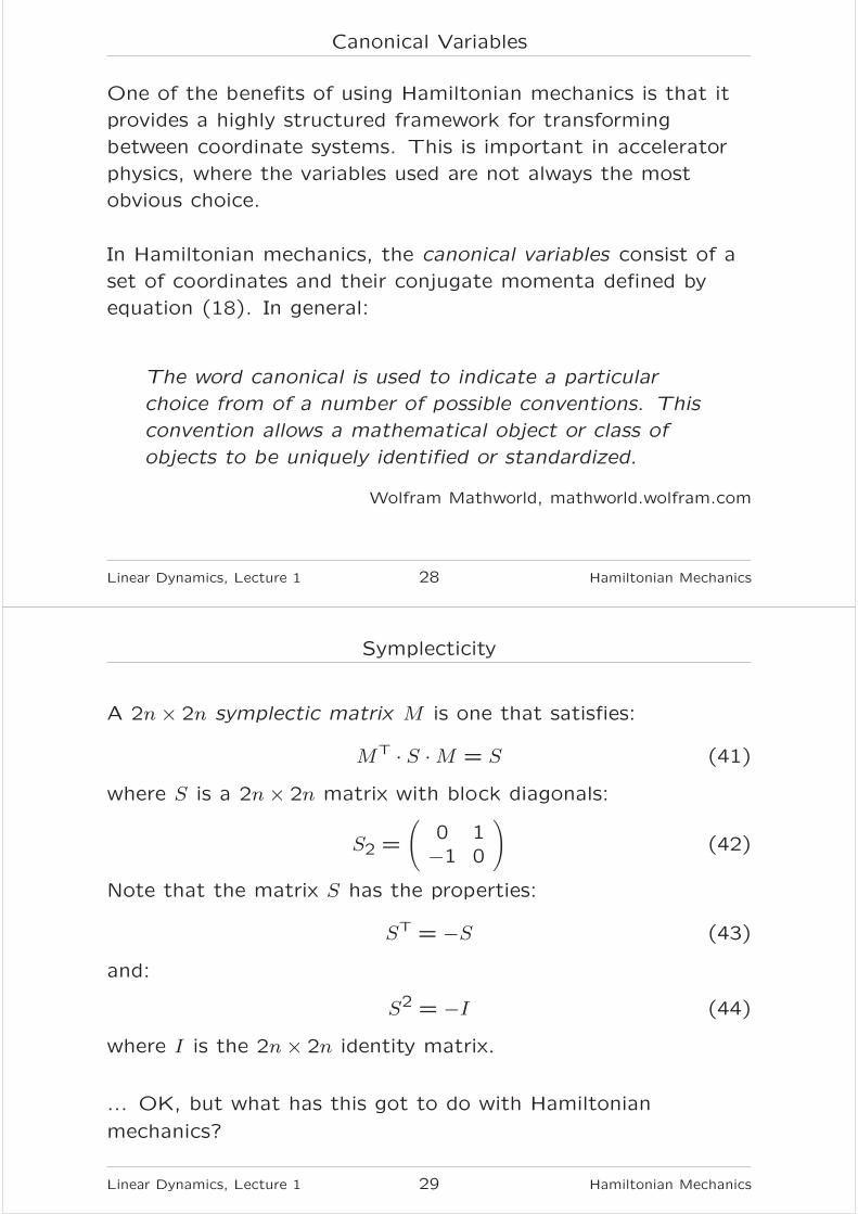
Canonical Variables
One of the benefits of using Hamiltonian mechanics is that it
provides a highly structured framework for transforming
between coordinate systems. This is important in accelerator
physics, where the variables used are not always the most
obvious choice.
In Hamiltonian mechanics, the canonical variables consist of a
set of coordinates and their conjugate momenta defined by
equation (18). In general:
The word canonical is used to indicate a particular
choice from of a number of possible conventions. This
convention allows a mathematical object or class of
objects to be uniquely identified or standardized.
Wolfram Mathworld, mathworld.wolfram.com
Linear Dynamics, Lecture 1 28 Hamiltonian Mechanics
Symplecticity
A 2n× 2n symplectic matrix M is one that satisfies:
MT · S ·M = S (41)
where S is a 2n× 2n matrix with block diagonals:
S2 =
(
0 1−1 0
)
(42)
Note that the matrix S has the properties:
ST = −S (43)
and:
S2 = −I (44)
where I is the 2n× 2n identity matrix.
... OK, but what has this got to do with Hamiltonian
mechanics?
Linear Dynamics, Lecture 1 29 Hamiltonian Mechanics
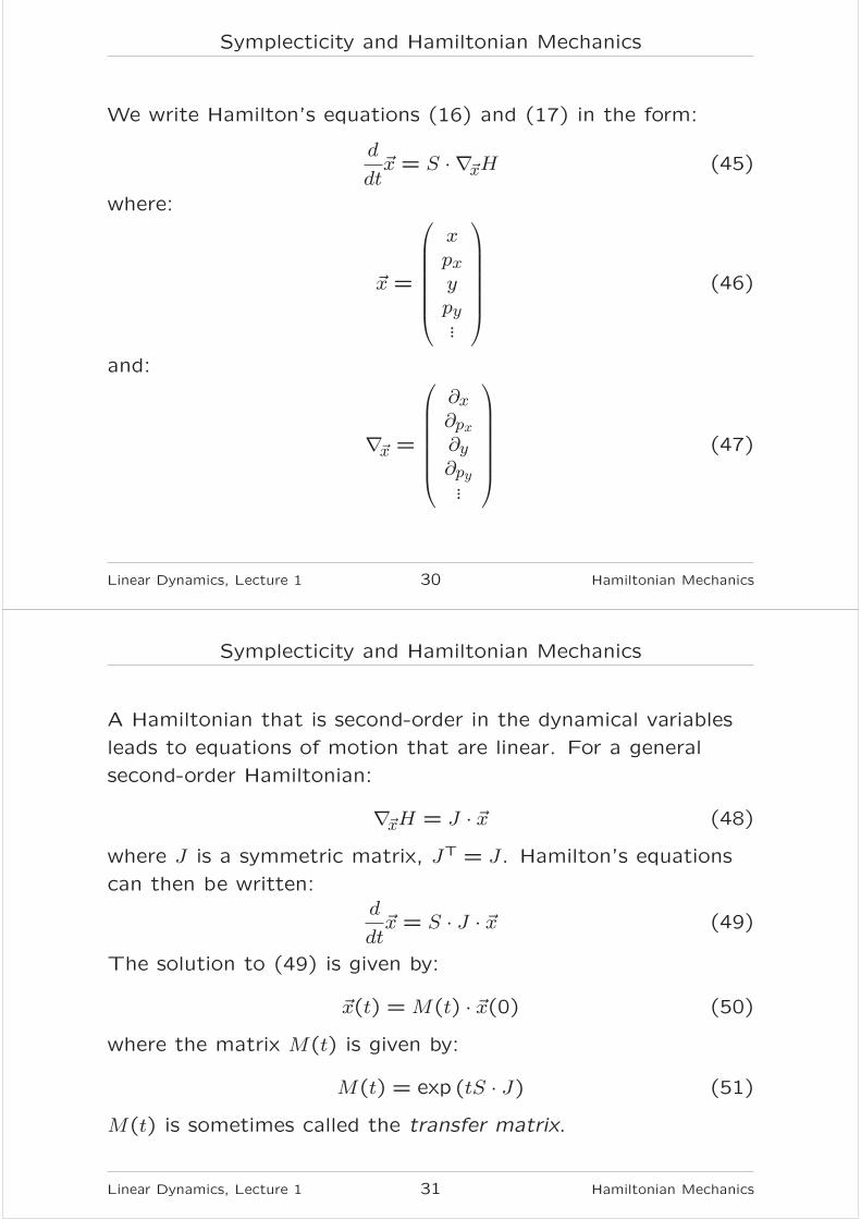
Symplecticity and Hamiltonian Mechanics
We write Hamilton’s equations (16) and (17) in the form:
d
dt~x = S · ∇~xH (45)
where:
~x =
x
pxy
py...
(46)
and:
∇~x =
∂x∂px∂y∂py...
(47)
Linear Dynamics, Lecture 1 30 Hamiltonian Mechanics
Symplecticity and Hamiltonian Mechanics
A Hamiltonian that is second-order in the dynamical variables
leads to equations of motion that are linear. For a general
second-order Hamiltonian:
∇~xH = J · ~x (48)
where J is a symmetric matrix, JT = J. Hamilton’s equations
can then be written:d
dt~x = S · J · ~x (49)
The solution to (49) is given by:
~x(t) = M(t) · ~x(0) (50)
where the matrix M(t) is given by:
M(t) = exp (tS · J) (51)
M(t) is sometimes called the transfer matrix.
Linear Dynamics, Lecture 1 31 Hamiltonian Mechanics

Symplecticity and Hamiltonian Mechanics
Now, note that J is symmetric and S is antisymmetric:
JT = J ST = −S (52)
Also, it can be shown (see Appendix B) that:
S · exp (tS · J) = exp (tJ · S) · S (53)
Using equations (52) and (53), we can write:
MT(t) · S ·M(t) = exp (−tJ · S) · S · exp (tS · J) (54)
= exp (−tJ · S) · exp (tJ · S) · S (55)
= S (56)
Therefore, from (41), M(t) is symplectic.
Conclusion: for a linear system whose dynamics can be
described by a Hamiltonian, the transfer matrix is symplectic.
... OK, but what does symplecticity mean physically?
Linear Dynamics, Lecture 1 32 Hamiltonian Mechanics
Symplecticity and Hamiltonian Mechanics
Consider an area of phase space (a plot of the conjugate
momentum vs the corresponding coordinate) defined by vectors
~e1 and ~e2.
Linear Dynamics, Lecture 1 33 Hamiltonian Mechanics
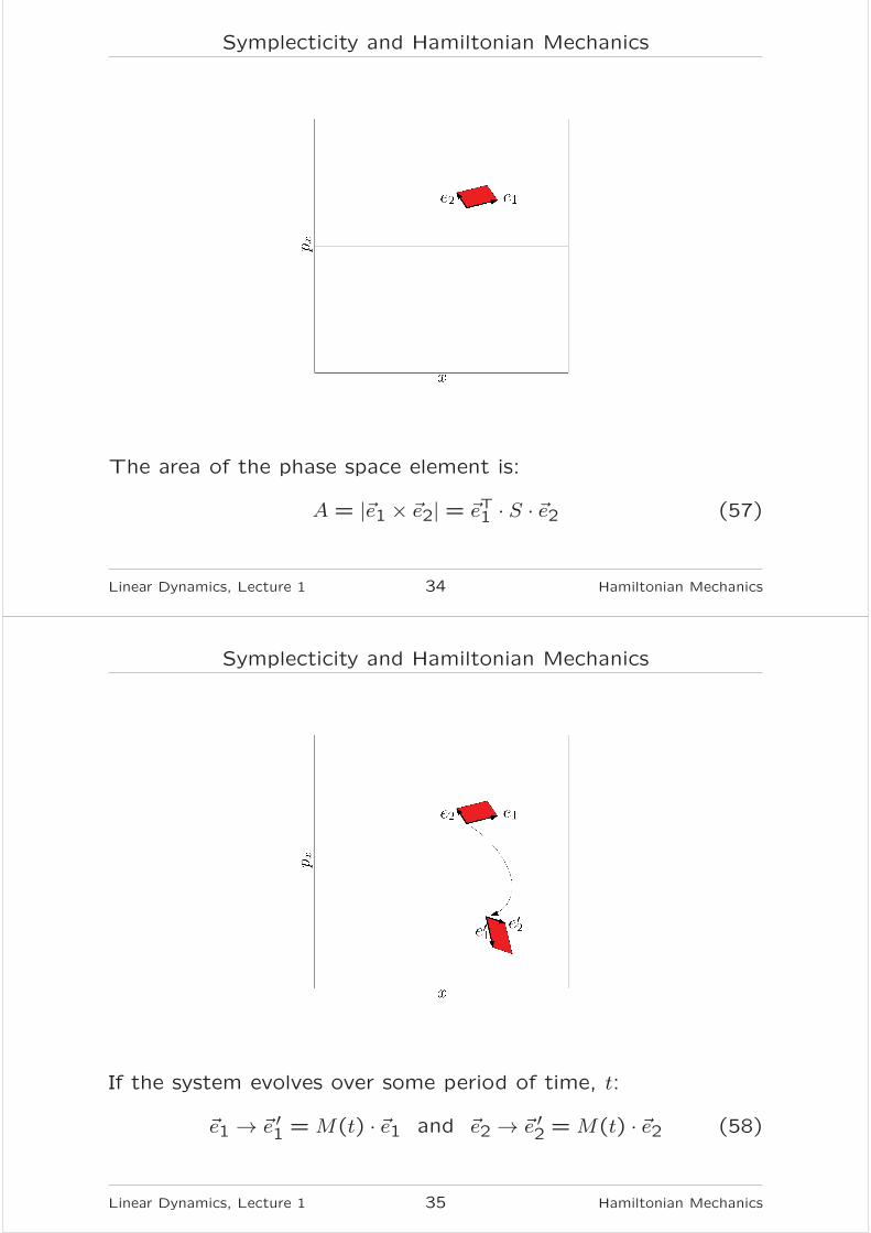
Symplecticity and Hamiltonian Mechanics
The area of the phase space element is:
A = |~e1 × ~e2| = ~eT1 · S · ~e2 (57)
Linear Dynamics, Lecture 1 34 Hamiltonian Mechanics
Symplecticity and Hamiltonian Mechanics
If the system evolves over some period of time, t:
~e1 → ~e ′1 = M(t) · ~e1 and ~e2 → ~e ′2 = M(t) · ~e2 (58)
Linear Dynamics, Lecture 1 35 Hamiltonian Mechanics
Symplecticity and Hamiltonian Mechanics
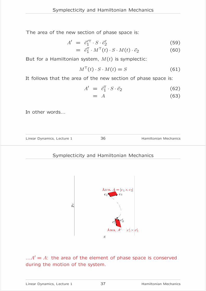
The area of the new section of phase space is:
A′ = ~e ′T1 · S · ~e ′2 (59)
= ~eT1 ·MT(t) · S ·M(t) · ~e2 (60)
But for a Hamiltonian system, M(t) is symplectic:
MT(t) · S ·M(t) = S (61)
It follows that the area of the new section of phase space is:
A′ = ~eT1 · S · ~e2 (62)
= A (63)
In other words...
Linear Dynamics, Lecture 1 36 Hamiltonian Mechanics
Symplecticity and Hamiltonian Mechanics
...A′ = A: the area of the element of phase space is conserved
during the motion of the system.
Linear Dynamics, Lecture 1 37 Hamiltonian Mechanics

Symplecticity and Hamiltonian Mechanics
Joseph Liouville, 1809-1882
We have shown that the area of phase space “elements” is
conserved during the motion of any system whose dynamics are
linear, and can be described by a Hamiltonian.
In fact, it can be shown that areas of phase space elements are
conserved for all Hamiltonian systems, even when the dynamics
are nonlinear. This important result is known as “Liouville’s
Theorem”.
Linear Dynamics, Lecture 1 38 Hamiltonian Mechanics
Symplecticity and Hamiltonian Mechanics
The conservation of area in phase space is an important
property of Hamiltonian systems, which are also known as
“conservative systems”. Not all dynamical systems are
conservative. The presence of dissipative forces, such as
friction, leads to a shrinkage of phase space area.
In accelerator physics, the phase space area occupied by a
bunch of particles is an important quantity, and is known as the
“emittance”. In an accelerator, synchrotron radiation can be
analogous to friction, and can reduce the emittance of a bunch
of particles. However, in many cases, it is a good
approximation to neglect non-conservative forces on particles in
an accelerator; in this approximation, Liouville’s theorem tells
us that the emittance of a bunch of particles is conserved as
the particles move through an accelerator.
Linear Dynamics, Lecture 1 39 Hamiltonian Mechanics

Canonical Transformations
One of the great advantages of Hamiltonian mechanics, is that
it provides a rigorous framework for making changes of
variables, and for writing down the equations of motion in the
new variables. In Hamiltonian mechanics, the process of
changing from one set of (canonical) variables to another is
known as a “canonical transformation”.
Here, we do not go through a rigorous treatment, but simply
quote some useful results, and give some examples.
In general, we wish to transform from a set of “old” canonical
variables (q,p) to a “new” set (Q,P). We wish to find
expressions for the new variables in terms of the old variables;
the requirement that the new variables be canonical is a
constraint on the expressions that are allowed.
Linear Dynamics, Lecture 1 40 Hamiltonian Mechanics
Canonical Transformations
Canonical transformations may be found by means of
“generating functions”. A generating function is a function of
some combination of old and new canonical variables, and
(optionally) the independent variable, t. For example, consider:
F2 = F2(q,P, t) (64)
F2 is a function of the old coordinates, the new momenta, and
the time. The old momenta are expressed as:
pi =∂F2
∂qi(65)
and the new coordinates are expressed as:
Qi =∂F2
∂Pi(66)
The new Hamiltonian is given by:
K = H +∂F2
∂t(67)
Linear Dynamics, Lecture 1 41 Hamiltonian Mechanics

Canonical Transformations
Let’s consider a concrete example. Consider the Hamiltonian
for a certain nonlinear oscillator:
H =p2
2(1 + q2)2+
1
2
(
q +1
3q3)2
(68)
If you like, you can write down the equations of motion using
Hamilton’s equations (16) and (17), and then try to solve
them. I prefer a simpler method. Write down the generating
function:
F2(q, P ) =
(
q +1
3q3)
P (69)
In this case, the generating function F2 is independent of time,
t. We can use F2(q, P ) to generate new canonical variables
(Q,P ), and a new Hamiltonian. If we’ve chosen the generating
function correctly, the equations of motion in the new variables
will be simpler to solve than the equations of motion in the old
variables. Let’s try...
Linear Dynamics, Lecture 1 42 Hamiltonian Mechanics
Canonical Transformations
Using the above equations (65) and (66), we find relations
between the old variables (q, p) and the new variables (Q,P ):
p =∂F2
∂q=(
1+ q2)
P (70)
Q =∂F2
∂P= q +
1
3q3 (71)
In other words:
P =p
1+ q2(72)
Q = q +1
3q3 (73)
and in terms of the new variables, the Hamiltonian (68)
becomes:
K =1
2P2 +
1
2Q2 (74)
Linear Dynamics, Lecture 1 43 Hamiltonian Mechanics

Canonical Transformations
Now the solution is easy. We recognise the Hamiltonian for a
simple harmonic oscillator, so the equations of motion can be
solved to give:
Q = Q0 sin(t+ φ0) (75)
where the constants Q0 and φ0 are set by the initial conditions.
In terms of the old coordinate:
q +1
3q3 = Q0 sin(t+ φ0) (76)
This is an algebraic equation, which we can solve for q. But
since this is a course on linear dynamics, we won’t take this
example any further.
Linear Dynamics, Lecture 1 44 Hamiltonian Mechanics
Canonical Transformations
Finally, we note that there are four “standard” mixed-variable
generating functions that can be used to construct canonical
transformations. The equations are as follows.
Generating function of the first kind:
F1 = F1(q,Q, t), pi =∂F1∂qi
, Pi = −∂F1∂Qi
, K = H + ∂F1∂t
(77)
Generating function of the second kind:
F2 = F2(q,P, t), pi =∂F2∂qi
, Qi =∂F2∂Pi
, K = H + ∂F2∂t
(78)
Generating function of the third kind:
F3 = F3(p,Q, t), qi = −∂F3∂pi
, Pi = −∂F3∂Qi
, K = H + ∂F3∂t
(79)
Generating function of the fourth kind:
F4 = F4(p,P, t), qi = −∂F4∂pi
, Qi =∂F4∂Pi
, K = H + ∂F4∂t
(80)
Linear Dynamics, Lecture 1 45 Hamiltonian Mechanics

Summary
Certain classical dynamical systems can be described using
Hamilton’s equations:
dx
dt=
∂H
∂px,
dpx
dt= −
∂H
∂x(81)
where (x, px) are dynamical variables (coordinate x and
conjugate or canonical momentum px); t is the independent
variable; the Hamiltonian H is a function (of the dynamical
variables) that defines the dynamics of the system.
Hamiltonian systems are symplectic: areas in phase space are
conserved as the system evolves (Liouville’s theorem).
We can change from one set of dynamical variables to another
using a formally defined canonical transformation. The new
variables defined by a canonical transformation also obey
Hamilton’s equations, for an appropriate Hamiltonian.
Linear Dynamics, Lecture 1 46 Hamiltonian Mechanics
Appendix A: Dynamics in an Electromagnetic Field
The Hamiltonian is:
H = p · x− L =(p− qA)2
2m+ qφ (82)
The first equation of motion (16) is easy enough:
dxi
dt=
∂H
∂pi=
pi − qAi
m(83)
This reduces to:
mxi = pi − qAi (84)
which we knew already from the definition of the conjugate
momentum (35).
The second equation of motion (17) needs some work...
Linear Dynamics, Lecture 1 47 Hamiltonian Mechanics

Appendix A: Dynamics in an Electromagnetic Field
Hamilton’s second equation (17) with the Hamiltonian (36)
gives for the x component of the momentum:
dpx
dt= −
∂H
∂x(85)
= q
(
x∂Ax
∂x+ y
∂Ay
∂x+ z
∂Az
∂x
)
− q∂φ
∂x(86)
Now, if we define a vector field:
B = ∇×A (87)
we notice that:
[x×B]x = x∂Ax
∂x+ y
∂Ay
∂x+ z
∂Az
∂x− x
∂Ax
∂x− y
∂Ax
∂y− z
∂Ax
∂z
=
(
x∂Ax
∂x+ y
∂Ay
∂x+ z
∂Az
∂x
)
−dAx
dt+
∂Ax
∂t(88)
Linear Dynamics, Lecture 1 48 Hamiltonian Mechanics
Appendix A: Dynamics in an Electromagnetic Field
It follows that we can write:
dpx
dt= q [x×B]x + q
dAx
dt− q
∂Ax
∂t− q
∂φ
∂x(89)
If we now define a vector field:
E = −∇φ−∂A
∂t(90)
then we can write:
d
dt(px − qAx) = q [x×B]x + qEx (91)
Finally, considering all vector components, we have:
d
dt(p− qA) = q (E+ x×B) (92)
Linear Dynamics, Lecture 1 49 Hamiltonian Mechanics

Appendix A: Dynamics in an Electromagnetic Field
Given the Hamiltonian (36):
H = p · x− L =(p− qA)2
2m+ qφ (93)
with the conjugate momentum (35):
p = mx+ qA (94)
the equation of motion from (17) is (92):
d
dt(p− qA) = q (E+ x×B) (95)
or:d
dtmx = q (E+ x×B) (96)
This is just Newton’s equation (1) with the Lorentz force (6).
Note that this was derived for non-relativistic particles: later we
will need to derive a relativistic equation of motion.
Linear Dynamics, Lecture 1 50 Hamiltonian Mechanics
Appendix B: Proof of Equation (53)
The matrix exponential exp(A) can be defined, as for the
exponential of a number, by the series:
exp(A) =∞∑
n=0
An
n!(97)
where An is the matrix power of A to the power n. Using (97)
we write:
S · exp (tS · J) = S ·
(
1+ tS · J +1
2t2S · J · S · J · · ·
)
(98)
Since S2 = −I, where I is the identity matrix, we can
post-multiply the right hand side of (98) by I = −S2:
S · exp (tS · J) = −S ·
(
1+ tS · J +1
2t2S · J · S · J · · ·
)
S2 (99)
Applying the initial factor −S and one final factor of S to each
term in the summation gives:
S · exp (tS · J) =
(
1+ tJ · S +1
2t2J · S · J · S · · ·
)
S
= exp (tJ · S) · S (100)
Linear Dynamics, Lecture 1 51 Hamiltonian Mechanics