Embed Size (px)
Citation preview
Review of the Primary National
Ambient Air Quality Standard for
Sulfur Oxides:
Risk and Exposure Assessment
Planning Document

[This page intentionally left blank.]
EPA-452/P-17-001
February 2017
Review of the Primary National Ambient Air Quality
Standard for Sulfur Oxides:
Risk and Exposure Assessment Planning Document
U.S. Environmental Protection Agency
Office of Air Quality Planning and Standards
Office of Air and Radiation
Research Triangle Park, North Carolina
i
DISCLAIMER
This document has been prepared by staff in the Health and Environmental Impacts
Division, Office of Air Quality Planning and Standards, U.S. Environmental Protection Agency
(EPA). Any findings and conclusions are those of the authors and do not necessarily reflect the
views of the Agency. This document is being circulated to facilitate discussion with the Clean
Air Scientific Advisory Committee and for public comment to inform the EPA’s consideration of
the primary national ambient air quality standard for sulfur oxides. This information is
distributed for the purposes of pre-dissemination peer review under applicable information
quality guidelines. It does not represent and should not be construed to represent any Agency
determination or policy.
Questions or comments related to this document should be addressed to Dr. Stephen
Graham, U.S. Environmental Protection Agency, Office of Air Quality Planning and Standards,
C539-07, Research Triangle Park, North Carolina 27711 (email: [email protected]) and
Dr. Nicole Hagan, U.S. Environmental Protection Agency, Office of Air Quality Planning and
Standards, C504-06, Research Triangle Park, North Carolina 27711 (email:
ii
TABLE OF CONTENTS
LIST OF FIGURES ...................................................................................................................... v
LIST OF TABLES ....................................................................................................................... vi
LIST OF ACRONYMS AND ABBREVIATIONS .................................................................. vii
EXECUTIVE SUMMARY .................................................................................................... ES-1
1 INTRODUCTION .............................................................................................................. 1-1
1.1 Background ................................................................................................................. 1-2
1.2 Conceptual Model for SO2 Exposure and Risk ........................................................... 1-3
REFERENCES ......................................................................................................................... 1-7
2 OVERVIEW OF THE PREVIOUS ASSESSMENT ...................................................... 2-1
2.1 Analysis Approach and Modeling Elements ............................................................... 2-1
2.1.1 Additional Analyses of Monitoring Data ............................................................... 2-3
2.1.2 Air Quality Scenarios ............................................................................................. 2-3
2.1.3 Benchmark Levels, Exposure-Response, and Risk Metrics .................................. 2-4
2.1.4 Relationship Between 1-Hour and 5-Minute Concentrations ................................ 2-6
2.2 Air Quality-Based Assessment ................................................................................... 2-6
2.2.1 Air Concentrations ................................................................................................. 2-7
2.2.2 Study Areas and Years ........................................................................................... 2-9
2.2.3 Comparison of Air Concentrations to Benchmarks ............................................... 2-9
2.2.4 Key Uncertainties and Limitations ...................................................................... 2-10
2.3 Risk and Exposure Assessment ................................................................................. 2-12
2.3.1 Study Areas, Time Period, and Simulated Population ......................................... 2-12
2.3.2 Exposure Modeling .............................................................................................. 2-13
2.3.2.1 Air Concentrations ........................................................................................... 2-15
2.3.2.2 Simulated Populations ...................................................................................... 2-16
2.3.2.3 Human Activity Patterns .................................................................................. 2-17
2.3.2.4 Microenvironmental Concentrations ................................................................ 2-18
2.3.2.5 Exposure Estimates .......................................................................................... 2-18
2.3.3 Health Risk Characterization ............................................................................... 2-19
2.3.4 Key Uncertainties and Limitations ...................................................................... 2-20
REFERENCES ....................................................................................................................... 2-24
3 CONSIDERATION OF THE NEWLY AVAILABLE INFORMATION .................... 3-1
iii
3.1 Key Considerations ..................................................................................................... 3-1
3.2 Health Effects Information .......................................................................................... 3-2
3.2.1 At-Risk Populations ............................................................................................... 3-3
3.2.2 Lung Function Decrements .................................................................................... 3-3
3.2.3 Other Endpoints ..................................................................................................... 3-4
3.3 Ambient Air Concentrations ....................................................................................... 3-5
3.3.1 Estimation of 5-Minute Concentrations ................................................................. 3-5
3.3.2 Characterizing the Spatial and Temporal Distribution of 1-hour SO2 Concentrations
................................................................................................................................ 3-7
3.4 Exposure Estimates ..................................................................................................... 3-7
3.4.1 Microenvironmental Concentrations ..................................................................... 3-8
3.4.2 Human Activity Patterns ........................................................................................ 3-8
3.4.3 Physical Attributes and Ventilation Rate ............................................................... 3-9
3.4.4 Exposure Estimate Bins ....................................................................................... 3-10
3.5 Conclusions ............................................................................................................... 3-10
REFERENCES ....................................................................................................................... 3-13
4 PLAN FOR THE CURRENT HEALTH RISK AND EXPOSURE ASSESSMENT ... 4-1
4.1 Population-based Exposure Assessment ..................................................................... 4-2
4.1.1 APEX Model Overview ......................................................................................... 4-3
4.1.2 Exposure Domain................................................................................................... 4-4
4.1.2.1 Study Areas and Time Periods ........................................................................... 4-4
4.1.3 SO2 Concentrations in Ambient Air ..................................................................... 4-12
4.1.3.1 Monitor Data Completeness Requirements...................................................... 4-12
4.1.3.2 Approach for Estimating Missing Values in Ambient Air Monitor Data ........ 4-13
4.1.3.3 AERMOD Predicted Concentrations ............................................................... 4-17
4.1.3.4 Adjusting Concentrations to Just Meet a Standard .......................................... 4-19
4.1.4 Microenvironmental Concentrations ................................................................... 4-22
4.1.5 At-Risk Populations ............................................................................................. 4-24
4.1.6 Simulated Individuals .......................................................................................... 4-24
4.1.6.1 Population Demographic Information .............................................................. 4-25
4.1.6.2 Asthma Prevalence ........................................................................................... 4-25
4.1.6.3 Commuting ....................................................................................................... 4-27
4.1.6.4 Human Activity Patterns .................................................................................. 4-27
iv
4.1.6.5 Personal Attributes ........................................................................................... 4-29
4.1.7 Exposure Assessment Estimates .......................................................................... 4-30
4.2 Health Risk Characterization .................................................................................... 4-31
4.2.1 Health Endpoints .................................................................................................. 4-31
4.2.2 Target Ventilation Rates ...................................................................................... 4-31
4.2.3 Exposure Benchmark-Based Health Risk ............................................................ 4-32
4.2.3.1 Benchmark Levels ............................................................................................ 4-32
4.2.3.2 Exposure Benchmark-based Risk Results ........................................................ 4-33
4.2.4 Lung Function Decrement-based Health Risk ..................................................... 4-34
4.2.4.1 Development of Exposure-Response Functions .............................................. 4-34
4.2.4.2 Lung Function Decrement-based Health Risk Results .................................... 4-39
4.3 Assessment of Variability and Characterization of Uncertainty ............................... 4-40
4.3.1 Assessment of Variability and Co-variability ...................................................... 4-41
4.3.2 Characterization of Uncertainty ........................................................................... 4-41
REFERENCES ....................................................................................................................... 4-44
LIST OF APPENDICES
A. Consideration of Support in Newly Available Information for Quantitative Assessment of
Other Asthma-Related Health Outcomes
B. Occurrences of 5-Minute SO2 Concentrations of Interest in the Recent Ambient Air
Monitoring Data (2013-2015)
C. Comparisons of SO2 Hourly Concentration Distributions between High and Low Years in
2011-2015
v
LIST OF FIGURES
Figure 1-1. Conceptual model for exposure and associated health risk of SO2 in ambient air. .. 1-6
Figure 2-1. Overview of analysis approach for 2009 REA. Blue boxes indicate approach for
estimating air concentrations, purple boxes indicate exposure modeling, and red
dashed boxes indicate use of health effects information. ......................................... 2-3
Figure 3-1. Trend in number of monitors with 5-minute data. .................................................... 3-6
Figure 4-1. Overview of the analysis approach for the REA. ..................................................... 4-2
Figure 4-2. Map indicating approximate dimensions of potential model-based study area (blue
circles surrounding sources) and SO2 emission sources > 100 tons per year in Brown
County, WI. .............................................................................................................. 4-8
Figure 4-3. Map indicating approximate dimensions of potential model-based study area (blue
circles surrounding sources) and SO2 emission sources > 100 tons per year in
Cuyahoga County, OH. ............................................................................................. 4-9
Figure 4-4. Map indicating approximate dimensions of potential model-based study area (blue
circles surrounding sources) and SO2 emission sources > 100 tons per year in
Hillsborough County, FL. ....................................................................................... 4-10
Figure 4-5. Map indicating approximate dimensions of a potential model-based study area (blue
circles surrounding sources) and SO2 emission sources > 100 tons per year in Marion
County, IN. ............................................................................................................. 4-11
Figure 4-6. Comparison of low and high concentration years using recent data (2011-2015) for
daily maximum 1-hour SO2 concentrations in ambient air in Hillsborough County,
FL (top left), Cuyahoga County, OH (top right), and Marion County, IN (bottom
left), and Brown County, WI (bottom right)........................................................... 4-21
Figure 4-7. Percent of individuals experiencing changes in sRaw ≥ 100% using controlled
human exposure study data (Table 4-6) fit using a probit regression (solid line).
Annotated with the number of study subjects from each study, dashed line indicates a
5th and 95th percentile prediction interval for the mean. Models for SO2 exposures
from 200-1,000 ppb (top panel) and for SO2 exposures from 200-600 ppb (bottom
panel). ..................................................................................................................... 4-38
vi
LIST OF TABLES
Table 2-1. Air quality scenarios evaluated in the 2009 REA. .................................................... 2-4
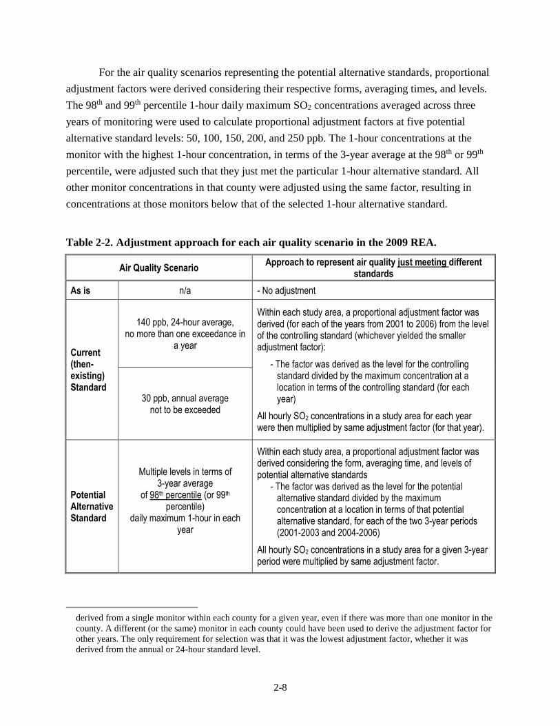
Table 2-2. Adjustment approach for each air quality scenario in the 2009 REA. ..................... 2-8
Table 4-1. Candidate study areas that meet the air quality, design value, and population criteria.
............................................................................................................................ 4-7
Table 4-2. Descriptive statistics for evaluating the approach used to substitute missing 1-hour
and 5-minute maximum concentrations using a monitor in Cuyahoga County, OH
(ID 390350038): all available measurements (no substitution) and that supplemented
with data where missing values were present. ........................................................ 4-14
Table 4-3. Example of estimated continuous 5-minute concentrations for hours for which only
the maximum 5-minute and 1-hour average concentrations are known and using
equation 4-1 or equation 4-2. .................................................................................. 4-16
Table 4-4. Example of estimated continuous 5-minute concentrations for hours for which more
than one 5-minute concentration and the 1-hour average concentration are known
and using equation 4-3. ........................................................................................... 4-17
Table 4-5. Estimated asthma prevalence for children and adults in four potential study areas. .....
.......................................................................................................................... 4-27
Table 4-6. Summary of controlled human exposure studies containing individual response data:
number and percent of individuals who experienced greater than or equal to a 100 or
200 percent increase in specific airway resistance (sRaw), adjusted for effects of
exercise in clean air. ............................................................................................... 4-37
Table 4-7. Estimated percent of the population experiencing sRaw ≥ 100% considered at 5 ppb
increments and using two different data sets to derive the E-R function: one using all
SO2 exposures, the other using only SO2 exposures between 200-600 ppb. .......... 4-39
vii
LIST OF ACRONYMS AND ABBREVIATIONS
APEX Air Pollutants Exposure model
AQS Air Quality System
BSA body surface area
CAA Clean Air Act
CASAC Clean Air Scientific Advisory Committee
CHAD Consolidated Human Activity Database
EGU Electricity generating unit
EPA Environmental Protection Agency
EVR equivalent ventilation rate
FEV1 forced expiratory volume in one minute
FR Federal Register
IRP Integrated Review Plan
ISA Integrated Science Assessment
ME microenvironment
MET metabolic equivalent of task
MSA metropolitan statistical area
NAAQS National Ambient Air Quality Standard
NEI National Emissions Inventory
NHANES National Health and Nutrition Examination Survey
NHIS National Health Interview Survey
NO2 nitrogen dioxide
O3 ozone
OAQPS Office of Air Quality Planning and Standards
ppb parts per billion
PA Policy Assessment
PM particulate matter
PMR peak-to-mean ratio
PRB policy-relevant background
REA Risk and Exposure Assessment
RMR resting metabolic rate
SO2 sulfur dioxide
SOX oxides of sulfur
sRaw specific airway resistance
V̇E activity-specific ventilation rate
ES-1
EXECUTIVE SUMMARY
The U.S. Environmental Protection Agency (EPA) is conducting a review of the air
quality criteria and the primary (health-based) national ambient air quality standard (NAAQS)
for sulfur oxides as described in the 2014 Integrated Review Plan for the Primary National
Ambient Air Quality Standard for Sulfur Dioxide. Based on analysis of the information available
in this review with regard to support for a quantitative risk and exposure assessment (REA) to
inform the review, this document outlines a plan, including scope and methods, for a REA. The
information considered includes the currently available scientific evidence, as assessed in the
second draft Integrated Science Assessment for Sulfur Oxides – Health Criteria (ISA), relevant
tools or methodologies, and other information or data, including that which is newly available in
this review.
As in the last review of the primary sulfur dioxide (SO2) standards, which was completed
in 2010, the health effects evidence available in this review indicates that short-term exposures
are causally linked to respiratory effects and that people with asthma are the at-risk population.
Specifically, controlled human exposure studies demonstrate an increased risk of lung function
decrements for people with asthma exposed while at increased ventilation rates. The plan for the
REA is based on these findings. This is similar to the REA conducted as part of the last review
(2009 REA), which included quantitative analyses of both exposure and risk. Specifically, the
2009 REA included: analyses focused on short-term (5-minute) SO2 concentrations; an exposure
assessment designed to estimate exposures likely to be experienced by at-risk populations while
at increased ventilation; and risk characterization utilizing two types of metrics: (1) comparisons
of exposures to concentrations of potential concern (benchmark levels), and (2) lung function
risk estimates.
This document and the planned quantitative analyses reflect several important new pieces
of information that can be used to address areas of uncertainty in the last review. Perhaps most
importantly, the plan for the REA outlined in this document focuses on the updated SO2 air
monitoring dataset available in this review. Specifically, the data for 5-minute concentrations are
greatly expanded with regard to both the number of monitoring locations for which hourly
maximum 5-minute concentrations are available and the number for which all 5-minute values
for each hour are available. Limitations in the 5-minute dataset available at the time of the last
review influenced the approaches that could be used in the 2009 REA to characterize the
potential for at-risk populations to experience exposures of potential concern. The analysis
approach for the new REA will be based on linking the health effects information to population
exposure estimates that draw on this improved understanding of 5-minute concentrations of SO2
ES-2
in the ambient air and will also take advantage of a number of improvements and updates to the
air quality, exposure, and risk models, and associated input data.
As in the last review, EPA intends to use the Air Pollutant Exposure model (APEX) to
estimate population exposures that account for the time people spend in different
microenvironments, as well as for time spent at elevated ventilation rates while exposed to peak
5-minute SO2 concentrations. The new REA will also reflect the new information and model
improvements now available including:
A SO2 air monitoring dataset that is greatly expanded with regard to both the number
of monitoring locations for which hourly maximum 5-minute concentrations are
available and the number for which all 5-minute values for each hour are available;
Improvements in the air quality dispersion model, AERMOD, intended to reduce
uncertainties in 1-hour concentration estimates;
Greatly expanded database of activity diaries, providing a stronger foundation for
population exposure modeling;
Improvements to several aspects of APEX; and,
Use of an expanded dataset for development of a lung function exposure-response
function, addressing uncertainty in the shape of the response function across the range
of the study data.
The results from a new REA are expected to provide an improved characterization of exposure
and risk to inform EPA’s review of the primary SO2 standard.
Plans for the exposure-based risk assessment include assessment of recent air quality
conditions and conditions just meeting the current standard in several study areas.1 The study
areas will be selected based on consideration of the magnitude of current SO2 concentrations,
number of monitors in the area, including those with 5-minute monitoring data, and population
size. The risk characterization will be based on both comparisons of population 5-minute
exposures at elevated ventilation to health-based benchmark levels and estimated population risk
of “moderate” or greater SO2-related lung function decrements. The analyses and results will be
documented in a REA. Key findings of the REA will then be considered in the broader context of
the Policy Assessment, which will also consider the current evidence as assessed in the ISA and
characterization of SO2 concentrations in ambient air across the U.S. based on recent monitoring
data, with particular attention to peak 5-minute concentrations. The Policy Assessment provides
staff analysis and conclusions regarding policy implications of the full array of currently
available information in each NAAQS review for consideration by the Administrator.
1 The need for additional air quality scenarios will be considered in the draft Policy Assessment that will accompany
the draft REA presenting results for the analyses described in this REA Planning Document.
1-1
1 INTRODUCTION
The U.S. Environmental Protection Agency (EPA) is conducting a review of the air
quality criteria and the primary (health-based)2 national ambient air quality standard (NAAQS)
for sulfur oxides (SOX). The purpose of this planning document (titled Review of the Primary
National Ambient Air Quality Standard for Sulfur Oxides: Risk and Exposure Assessment
Planning Document – hereafter referred to as REA Planning Document) is to describe the
consideration of the extent to which newly available scientific evidence, tools or methodologies,
or information warrant the conduct of a quantitative risk and exposure assessment (REA) that
might inform this review. Also considered is the extent to which newly available evidence may
refine our3 characterization of exposure and risk estimates provided by the assessments
conducted for the last review. Based on these considerations, and as described below, we plan to
develop a new REA to inform the current review of the primary NAAQS for SOX. Accordingly,
this document’s additional purpose is to describe the general plan, including scope and methods
for conducting the REA.
In the last review, while the EPA made a number of revisions to the standards, it also
affirmed sulfur dioxide (SO2) as the indicator for the NAAQS for SOx based on its more
common occurrence in the atmosphere and the predominance of SO2 studies in the health effects
information for SOx (34 FR 1988, February 11, 1969; 75 FR 35520, June 22, 2010). The EPA
also promulgated a new 1-hour standard to afford the requisite protection for at-risk populations
such as people with asthma against an array of adverse respiratory health effects related to short-
term SO2 exposures. The 1-hour standard was set at a level of 75 parts per billion (ppb), based on
the 3-year average of the annual 99th percentile of 1-hour daily maximum SO2 concentrations.
The EPA also revoked the then-existing 24-hour and annual primary standards based largely on
the conclusion that the 1-hour standard would also control longer-term average concentrations,
maintaining 24-hour and annual concentrations generally well below the levels of those
standards, and on the lack of evidence indicating the need for such longer-term standards.
In conjunction with the revisions to the standards, the EPA required that monitoring
agencies report 5-minute SO2 measurements, either the highest 5-minute concentration for each
hour of the day or all twelve 5-minute concentrations for each hour of the day. The rationale for
2 The EPA is separately reviewing the welfare effects associated with sulfur oxides and the public welfare protection
provided by the secondary SO2 standard, in conjunction with a review of the secondary standards for nitrogen
oxides and PM with respect to their protection of the public welfare from adverse effects related to ecological
effects (U.S. EPA, 2017).
3 In this document, the terms “staff,” “we” and “our” refer to staff in the EPA’s Office of Air Quality Planning and
Standards (OAQPS).
1-2
this requirement was to provide additional monitoring data for use in subsequent reviews of the
primary standard, particularly in considering the extent of protection provided by the 1-hour
standard against 5-minute peak SO2 concentrations of concern (75 FR 35554, June 22, 2010).
These measurements are among the information newly available in this review that is considered
in this document.
This document presents a critical evaluation of information related to SO2 human
exposure and risk newly available in the second draft of the Integrated Science Assessment for
Sulfur Oxides – Health Criteria (U.S. EPA, 2016; hereafter referred to as second draft ISA).
Advances in modeling tools and techniques and air quality data that have become available since
the last review are also considered. This document is intended to facilitate consultation with the
Clean Air Scientific Advisory Committee (CASAC), as well as an opportunity for public
participation, on this evaluation of the potential support in the current information for updated
quantitative analyses of SO2 exposures and/or health risks, and on the plan for such analyses, as
warranted. This evaluation has considered the degree to which newly available scientific
evidence, tools or methodologies, or information may address or improve our consideration of
important uncertainties associated with the analyses from the last review (summarized in chapter
2). Based on these considerations and our preliminary conclusions on the extent to which
updated quantitative analyses of exposures and/or health risks are warranted in the current
review (chapter 3), this document presents general plans for such analyses (chapter 4).
1.1 BACKGROUND
Sections 108 and 109 of the Clean Air Act (CAA) govern the establishment and periodic
review of the NAAQS. Section 108 [42 U.S.C. 7408] directs the Administrator to identify and
list certain air pollutants and then to issue air quality criteria for those pollutants. The
Administrator is to list those air pollutants that in his “judgment, cause or contribute to air
pollution which may reasonably be anticipated to endanger public health or welfare,” “the
presence of which in the ambient air results from numerous or diverse mobile or stationary
sources;” and “for which…[the Administrator] plans to issue air quality criteria…” CAA section
108(a)(1). The NAAQS are established for these pollutants. The CAA requires that NAAQS are
to be based on air quality criteria, which are intended to “accurately reflect the latest scientific
knowledge useful in indicating the kind and extent of all identifiable effects on public health or
welfare that may be expected from the presence of [the] pollutant in the ambient air…” CAA
section 108(a)(2). Under CAA section 109 [42 U.S.C. 7409], the EPA Administrator is to
propose, promulgate, and periodically review, at five-year intervals, “primary” (health-based)
1-3
and “secondary” (welfare-based)4 NAAQS for such pollutants for which air quality criteria are
issued.5 Based on periodic reviews of the air quality criteria and standards, the Administrator is
to make revisions in the criteria and standards, and promulgate any new standards, as may be
appropriate. The CAA also requires that an independent scientific review committee review the
air quality criteria and standards and recommend to the Administrator any new standards and
revisions of existing air quality criteria and standards as may be appropriate, a function now
performed by the CASAC.
The overall plan for this review was presented in the Integrated Review Plan for the
Primary National Ambient Air Quality Standard for Sulfur Dioxide (U.S. EPA, 2014, hereafter
referred to as IRP). That plan discusses the preparation of key documents in the NAAQS review
process including an Integrated Science Assessment (ISA), a Risk and Exposure Assessment
(REA; as warranted), and a Policy Assessment (PA). In general terms, the ISA is to provide a
critical assessment of the latest available scientific information upon which the NAAQS are to be
based, and the Policy Assessment is to evaluate the policy implications of the information
contained in the ISA and of any policy-relevant quantitative analyses, such as a quantitative
REA, that were performed for the review or for past reviews. Based on that evaluation, the
Policy Assessment presents staff conclusions regarding standard-setting options for the
Administrator to consider in reaching decisions on the NAAQS.6
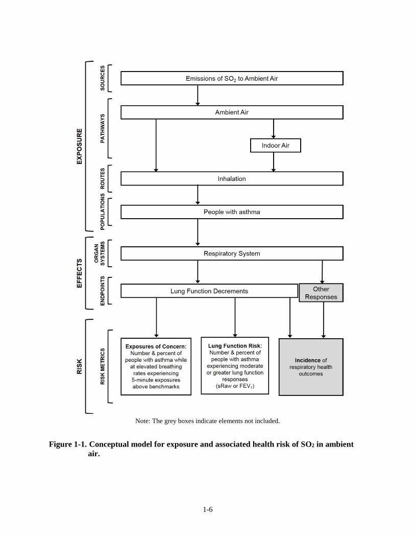
1.2 CONCEPTUAL MODEL FOR SO2 EXPOSURE AND RISK
This section describes the conceptual model for exposure and associated health risk of
SO2 in ambient air. The model summarizes our consideration of the currently available
information on emissions sources, exposure pathways, routes of exposure, exposed populations,
health endpoints and risk metrics. This general model, illustrated in Figure 1-1, guided our
4 Section 302(h) of the CAA provides that all language referring to effects on welfare includes but is not limited to,
“…effects on soils, water, crops, vegetation, man-made materials, animals, wildlife, weather, visibility and
climate, damage to and deterioration of property, and hazards to transportation, as well as effects on economic
values and on personal comfort and well-being…”
5 Section 109(b)(1) [42 U.S.C. 7409] of the CAA defines a primary standard as one “the attainment and maintenance
of which in the judgment of the Administrator, based on such criteria and allowing an adequate margin of safety,
are requisite to protect the public health.” Section 109(b)(2) of the CAA directs that a secondary standard is to
“specify a level of air quality the attainment and maintenance of which, in the judgment of the Administrator,
based on such criteria, is requisite to protect the public welfare from any known or anticipated adverse effects
associated with the presence of [the] pollutant in the ambient air.”
6 Review of NAAQS involve consideration of the four basic elements of a standard: indicator, averaging time, form,
and level. The indicator defines the pollutant to be measured in the ambient air for the purpose of determining
compliance with the standard. The averaging time defines the time period over which air quality measurements
are to be obtained and averaged or cumulated. The form of a standard defines the air quality statistic that is to be
compared to the level of the standard in determining whether an area attains the standard. The level of a standard
defines the air quality concentration used (i.e., an ambient air concentration of the indicator pollutant).
1-4
assessment in the last review and, as discussed in section 3.5 below, it remains appropriate in the
current review.
Exposure pathways relevant for SO2 are impacted by emissions sources, chemistry,
meteorology, and ambient air concentrations. Anthropogenic SO2 emissions originate primarily
from point sources, including coal-fired electricity generating units (EGUs) and other industrial
facilities (U.S. EPA 2008 [hereafter referred to as the 2008 ISA], section 2.1; second draft ISA,
section 2.2.1). The point source nature of these emissions contribute to the relatively high spatial
variability of SO2 concentrations (both ambient air and exposure) compared with pollutants such
as particulate matter (PM) and ozone (O3) (second draft ISA, section 3.2.3). Another contributing
factor to spatial variability is the dispersion and oxidation of SO2 in the atmosphere, resulting in
decreasing SO2 concentrations with increasing distance from the source. SO2 travels as a plume
which may or may not impact large portions of surrounding populated areas depending on
meteorological conditions. Concentrations of SO2 in ambient air do not exhibit consistently
strong temporal variability over daily or seasonal time scales, although in some areas
concentrations are low during nighttime and show a daytime maximum, impacting temporal
exposure patterns (2008 ISA, Figure 2-24; second draft ISA, Figures 2-26 and 2-27). The largest
natural sources of SO2 are volcanoes and wildfires. Indoor SO2 sources can include secondary
heating sources (e.g., fireplaces, space heaters), however, personal SO2 exposure measurements
have generally been lower than ambient air concentrations, indicating personal exposure to
generally be dominated by ambient air exposure (2008 ISA, section 2.6.3; second draft ISA,
section 3.4.1). The information newly available in this review supports, and in some cases
augments with more detail (e.g., more extensive ambient monitoring information), these aspects
our conceptual model.
Regarding exposed populations and health endpoints, the 2009 REA focused on lung
function decrements in people with asthma while at moderate or greater exertion. This reflected
the 2008 ISA conclusion there was sufficient evidence to infer a causal relationship between
respiratory morbidity and short-term (5-minutes to 24-hours) exposure to SO2. Key supporting
evidence came from controlled human exposure studies that showed lung function decrements
(as measured by reductions in forced expiratory volume, FEV1, and increased specific airway
resistance, sRaw) and respiratory symptoms in adult individuals with asthma exposed to SO2 for
5-10 minutes while at elevated breathing rates (2008 ISA, section 5.2; second draft ISA, section
5.2).7 As discussed in section 3.2, the information available in this review continues to support
these primary health effects conclusions and their inclusions in the conceptual model.
7 These aspects of the health effects evidence and its use in the 2009 REA are summarized in section 2.2.3.
1-5
In the last review, risks of these health effects to this at-risk population were
characterized through two types of metrics. The first was characterization of the extent to which
individuals with asthma were estimated to experience 5-minute exposures at or above
concentrations of potential concern (based on benchmark levels described in section 2.2.3) while
they were at elevated breathing rates. The assessment also characterized the extent to which
individuals with asthma were estimated to experience moderate or greater lung function
responses (as measured by FEV1 or sRaw) as a result of 5-minute SO2 exposures while at
elevated breathing rates. As discussed in chapters 3 and 4, these types of risk metrics are also
considered for the current review.
1-6
Note: The grey boxes indicate elements not included.
Figure 1-1. Conceptual model for exposure and associated health risk of SO2 in ambient
air.
1-7
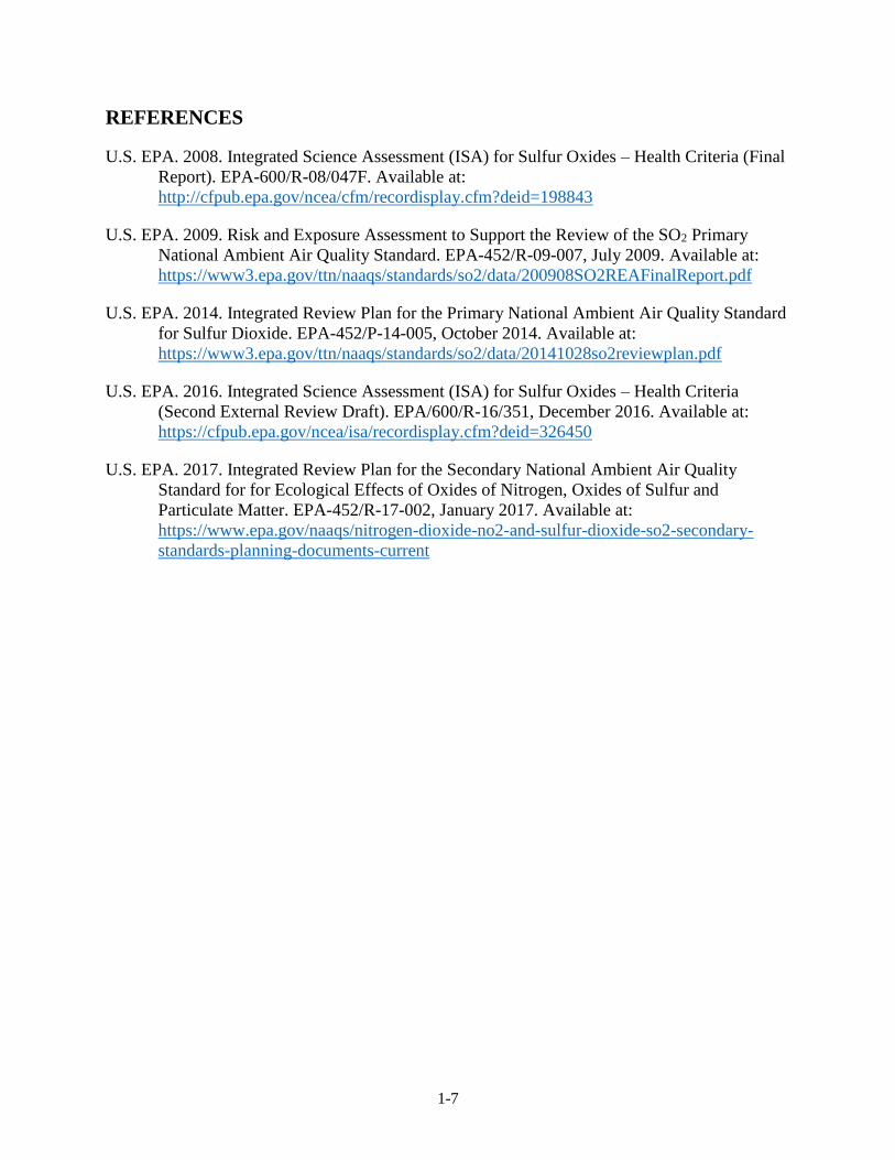
REFERENCES
U.S. EPA. 2008. Integrated Science Assessment (ISA) for Sulfur Oxides – Health Criteria (Final
Report). EPA-600/R-08/047F. Available at:
http://cfpub.epa.gov/ncea/cfm/recordisplay.cfm?deid=198843
U.S. EPA. 2009. Risk and Exposure Assessment to Support the Review of the SO2 Primary
National Ambient Air Quality Standard. EPA-452/R-09-007, July 2009. Available at:
https://www3.epa.gov/ttn/naaqs/standards/so2/data/200908SO2REAFinalReport.pdf
U.S. EPA. 2014. Integrated Review Plan for the Primary National Ambient Air Quality Standard
for Sulfur Dioxide. EPA-452/P-14-005, October 2014. Available at:
https://www3.epa.gov/ttn/naaqs/standards/so2/data/20141028so2reviewplan.pdf
U.S. EPA. 2016. Integrated Science Assessment (ISA) for Sulfur Oxides – Health Criteria
(Second External Review Draft). EPA/600/R-16/351, December 2016. Available at:
https://cfpub.epa.gov/ncea/isa/recordisplay.cfm?deid=326450
U.S. EPA. 2017. Integrated Review Plan for the Secondary National Ambient Air Quality
Standard for for Ecological Effects of Oxides of Nitrogen, Oxides of Sulfur and
Particulate Matter. EPA-452/R-17-002, January 2017. Available at:
https://www.epa.gov/naaqs/nitrogen-dioxide-no2-and-sulfur-dioxide-so2-secondary-
standards-planning-documents-current
2-1
2 OVERVIEW OF THE PREVIOUS ASSESSMENT
This chapter summarizes the assessment in the last review, which is described in more
detail in the Risk and Exposure Assessment to Support the Review of the SO2 Primary National
Ambient Air Quality Standards: Final Report from the last review (U.S. EPA 2009; hereafter
referred to as 2009 REA). This chapter begins with an overview of the analysis approach and
modeling elements in the last review (section 2.1). The overview section also describes, for the
last review, the analyses of monitoring data (section 2.1.1), air quality scenarios (section 2.1.2),
the health endpoint, concentration-response, and risk metrics (section 2.1.3), and the relationship
used to estimate 5-minute concentrations from 1-hour SO2 concentrations (section 2.1.4). Section
2.2 describes the air quality-based assessment and section 2.3 describes the risk and exposure
assessment for the last review, as well as the key uncertainties and limitations.
2.1 ANALYSIS APPROACH AND MODELING ELEMENTS
In each NAAQS review, selection of the approach most appropriate for the
characterization of risks is influenced by the nature and strength of the evidence for the subject
pollutant. Depending on the type of evidence available, analyses may include quantitative risk
assessments based on dose-response, exposure-response, or ambient air concentration-response
relationships. Analyses may also be based on comparisons of exposure estimates or ambient air
quality concentrations (i.e., as surrogates for potential ambient air exposures) with concentrations
of potential concern, based on findings of controlled human exposure studies. This section
summarizes the assessment approach (including discussion of key analysis steps) used in the last
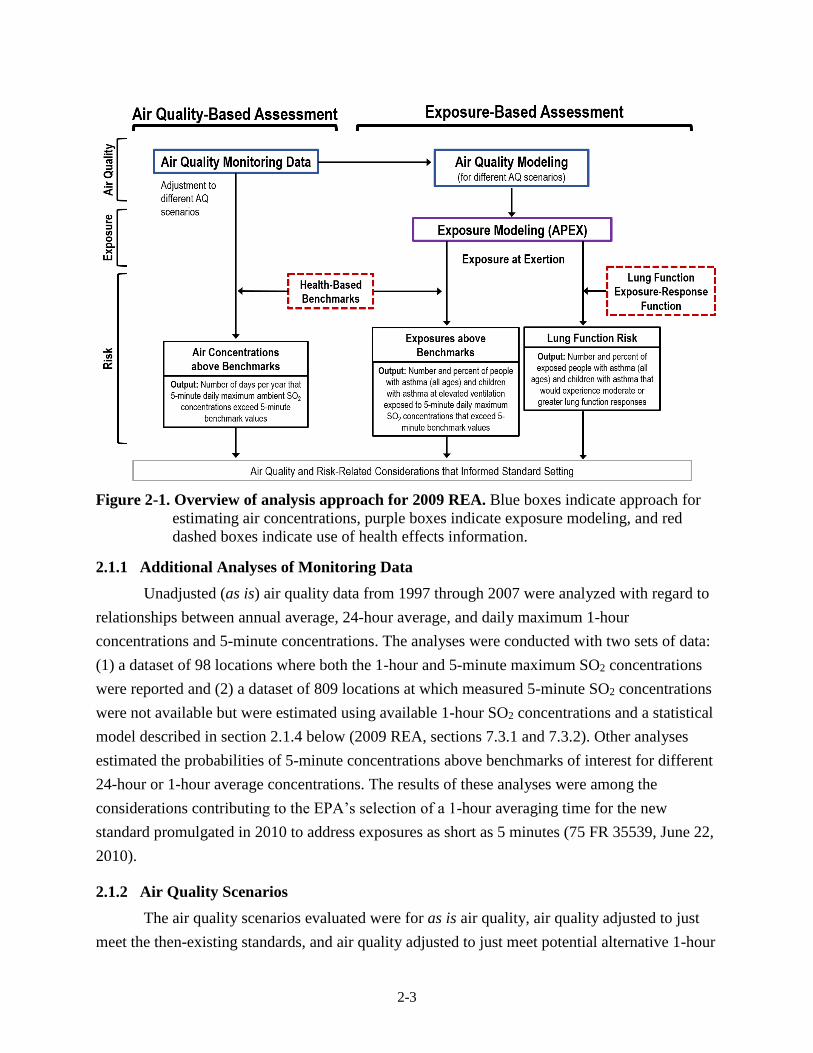
review. As illustrated in Figure 2-1, the REA completed for the 2010 review employed two
health risk approaches, one based on ambient air concentrations alone and the second
incorporating estimates of human exposure. Both approaches evaluated potential health risk
using several different air quality scenarios, including a scenario that considered unadjusted
ambient air concentrations (“as is” air quality) as well as scenarios that considered ambient air
concentrations adjusted to just meet the then-existing and several potential alternative standards
(see section 2.1.2 for details).
In the first assessment approach, SO2 concentrations at ambient air monitors were used as
a surrogate for exposure in 40 U.S. counties. This air quality-based assessment evaluated the
number of days (per monitor and per year) that daily 5-minute maximum SO2 concentrations in
ambient air exceeded the 5-minute concentrations of potential concern (referred to as
“benchmark levels”). Section 2.1.1 provides a brief summary of air quality analyses of the larger
set of ambient air monitoring data across the U.S. for the years 1997 through 2007. The air
2-2
quality-based assessment approach and the associated key uncertainties and limitations are
described in section 2.2.
In the exposure-based approach, risk was characterized two ways. For both, population-
based estimates of human exposure were developed using an exposure model in order to account
for time people spend in different microenvironments, as well as for time spent at elevated
ventilation rates while exposed to peak 5-minute SO2 concentrations. The model simulated
populations in two study areas: Greene County, MO and a three-county portion of the St. Louis
Metropolitan Statistical Area (MSA). The populations simulated included all people with
asthma, with results also presented particular to the subset of those that were children. Health
risk was characterized in the following ways:
Exposures Above Benchmarks: The 5-minute exposure concentrations of individuals at
elevated ventilation rates within each study area were compared to 5-minute benchmark
levels. The number and percent of people with asthma exposed, while at elevated
ventilation, to 5-minute daily maximum SO2 concentrations that exceeded the benchmark
levels were estimated for each air quality scenario.
Lung Function Risk: Lung function risk was estimated by combining the population-based
5-minute exposure estimates with two exposure-response (E-R) functions, also derived
from the controlled human exposure studies. Results were reported in terms of the
number and percent of exposed people with asthma estimated to experience moderate or
greater lung function responses (in terms of FEV1 and sRaw) at least once per year and
the total number of such lung function responses estimated to occur per year.
Details for these two health risk and exposure assessment approaches and the key associated
uncertainties and limitations are described in section 2.3.
2-3
Figure 2-1. Overview of analysis approach for 2009 REA. Blue boxes indicate approach for
estimating air concentrations, purple boxes indicate exposure modeling, and red
dashed boxes indicate use of health effects information.
2.1.1 Additional Analyses of Monitoring Data
Unadjusted (as is) air quality data from 1997 through 2007 were analyzed with regard to
relationships between annual average, 24-hour average, and daily maximum 1-hour
concentrations and 5-minute concentrations. The analyses were conducted with two sets of data:
(1) a dataset of 98 locations where both the 1-hour and 5-minute maximum SO2 concentrations
were reported and (2) a dataset of 809 locations at which measured 5-minute SO2 concentrations
were not available but were estimated using available 1-hour SO2 concentrations and a statistical
model described in section 2.1.4 below (2009 REA, sections 7.3.1 and 7.3.2). Other analyses
estimated the probabilities of 5-minute concentrations above benchmarks of interest for different
24-hour or 1-hour average concentrations. The results of these analyses were among the
considerations contributing to the EPA’s selection of a 1-hour averaging time for the new
standard promulgated in 2010 to address exposures as short as 5 minutes (75 FR 35539, June 22,
2010).
2.1.2 Air Quality Scenarios
The air quality scenarios evaluated were for as is air quality, air quality adjusted to just
meet the then-existing standards, and air quality adjusted to just meet potential alternative 1-hour
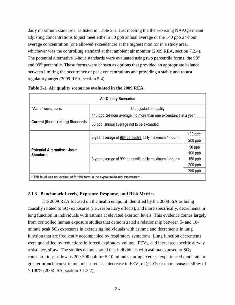
2-4
daily maximum standards, as listed in Table 2-1. Just meeting the then-existing NAAQS meant
adjusting concentrations to just meet either a 30 ppb annual average or the 140 ppb 24-hour
average concentration (one allowed exceedance) at the highest monitor in a study area,
whichever was the controlling standard at that ambient air monitor (2009 REA, section 7.2.4).
The potential alternative 1-hour standards were evaluated using two percentile forms, the 98th
and 99th percentile. These forms were chosen as options that provided an appropriate balance
between limiting the occurrence of peak concentrations and providing a stable and robust
regulatory target (2009 REA, section 5.4).
Table 2-1. Air quality scenarios evaluated in the 2009 REA.
Air Quality Scenarios
“As is” conditions Unadjusted air quality
Current (then-existing) Standards
140 ppb, 24-hour average, no more than one exceedance in a year
30 ppb, annual average not to be exceeded
Potential Alternative 1-hour Standards
3-year average of 98th percentile daily maximum 1-hour = 100 ppba
200 ppb
3-year average of 99th percentile daily maximum 1-hour =
50 ppb
100 ppb
150 ppb
200 ppb
250 ppb
a This level was not evaluated for this form in the exposure-based assessment.
2.1.3 Benchmark Levels, Exposure-Response, and Risk Metrics
The 2009 REA focused on the health endpoint identified by the 2008 ISA as being
causally related to SO2 exposures (i.e., respiratory effects), and more specifically, decrements in
lung function in individuals with asthma at elevated exertion levels. This evidence comes largely
from controlled human exposure studies that demonstrated a relationship between 5- and 10-
minute peak SO2 exposures in exercising individuals with asthma and decrements in lung
function that are frequently accompanied by respiratory symptoms. Lung function decrements
were quantified by reductions in forced expiratory volume, FEV1, and increased specific airway
resistance, sRaw. The studies demonstrated that individuals with asthma exposed to SO2
concentrations as low as 200-300 ppb for 5-10 minutes during exercise experienced moderate or
greater bronchoconstriction, measured as a decrease in FEV1 of ≥ 15% or an increase in sRaw of
≥ 100% (2008 ISA, section 3.1.3.2).
2-5
Among individuals with asthma, the 2008 ISA found that both the percent of individuals
affected and the severity of response increased with increasing SO2 concentrations across the
range studied. At concentrations ranging from 200-300 ppb, the lowest levels tested in free
breathing chamber studies,8 5-30% of exercising individuals with asthma experienced moderate
or greater decrements in lung function (2008 ISA, Table 3-1). At concentrations ≥ 400 ppb,
moderate or greater decrements in lung function occurred in 20-60% of exercising individuals
with asthma and a larger percentage of individuals with asthma experienced severe decrements
in lung function (i.e., ≥ 200% increase in sRaw, and/or ≥ 20% decrease in FEV1), compared to
exposures at 200-300 ppb (2008 ISA, Table 3-1). Additionally, at concentrations ≥ 400 ppb,
moderate or greater decrements in lung function were frequently accompanied by respiratory
symptoms (2008 ISA, Table 3-1).
These controlled human exposure study data were used in two ways: (1) to identify
exposure concentrations of potential concern (benchmark levels) and (2) to derive E-R functions
for lung function decrements. The benchmark levels were compared to SO2 air concentrations
and modeled estimates of human exposure (section 2.3.3 below) to characterize potential health
risks. The E-R functions were combined with outputs from the exposure modeling to
quantitatively estimate lung function risk for exposed individuals with asthma (section 2.3.4
below). The identification of potential health effect benchmarks and the derivation of the E-R
functions are briefly described below and more detailed information can be found in the 2009
REA.
The benchmark levels are concentrations chosen to represent “exposures of potential
concern” which were used in the analyses to estimate exposures and risks associated with 5-
minute concentrations of SO2 (75 FR 35527, June 22, 2010). Based on the evidence in the 2008
ISA and recommendations from the CASAC, staff concluded that it was appropriate to examine
5-minute benchmark levels in the range of 100-400 ppb (2009 REA, chapter 7). The comparisons
of SO2 concentrations to benchmark levels provided perspective on the extent to which, under
various air quality scenarios, there was the potential for at-risk populations to experience SO2
exposures that could be of concern.
8 In addition to “free-breathing” studies (i.e., studies in which individuals breathe the air while sequestered in a large
chamber), a limited number of studies assessed effects based on exposures delivered via mouthpiece breathing. A
few of these studies assessed exposure concentrations as low as 100 ppb (e.g., Sheppard et al. 1981 exposed two
subjects to 100 ppb SO2), although some methodological aspects of the studies limit the conclusions the ISA has
drawn from them. Further, such studies that utilize a mouthpiece exposure system cannot be directly compared to
studies involving freely breathing subjects, as nasal absorption of SO2 is bypassed during oral breathing, thus
allowing a greater fraction of inhaled SO2 to reach the tracheobronchial airways. As a result, individuals exposed
to SO2 through a mouthpiece are likely to experience greater respiratory effects from a given SO2 exposure
(second draft ISA, p. 5-22).
2-6
The exposure-based risk assessment also included two types of lung function responses
(i.e., sRaw and FEV1) and two levels of response (≥ 100% and 200% increase for sRaw and ≥
15% and 20% decrease for FEV1). The risk estimates were based on using two different
functional forms for the E-R function: a 2-parameter logistic model and a probit model. 9 Risk
estimates based on sRaw as the measure of lung function response were given primary emphasis
in the 2009 REA because the E-R relationships were developed using a greater number of
samples collected from individual subjects, which provided more confidence in the E-R
relationship when compared with that developed for the FEV1 health endpoint.10 Lung function
risk estimates were presented as a range based on using the two model forms. Risk was estimated
across the full range of estimated exposures, including exposure concentrations below those
assessed in the controlled human exposure studies (2009 REA, section 9.2.3).
2.1.4 Relationship Between 1-Hour and 5-Minute Concentrations
Based on the health effects information summarized above, the 2009 REA focused on
exposures and risk associated with 5-minute concentrations of SO2. While a majority of the then-
existing SO2 monitoring network sites reported 1-hour average SO2 concentrations, only a
limited number of ambient air monitors reported 5-minute maximum SO2 concentrations. A
statistical model was developed to extend the 5-minute SO2 air quality characterization to
locations where 1-hour average SO2 concentrations were reported and associated 5-minute
concentrations were not.
Peak-to-mean ratios (PMRs) were obtained by dividing the 5-minute maximum SO2
concentration occurring within an hour by the corresponding 1-hour SO2 concentration.
Distributions of PMRs were generated using 1-hour concentrations and categorical variables in
defining the distributions of PMRs. Using probabilistic sampling and this statistical relationship,
every 1-hour concentrations of SO2 at ambient air monitors and at air quality-modeled receptor
locations was assigned a 5-minute maximum SO2 concentration. More information about the
development and evaluation of PMRs is described in section 7.2.3 of the 2009 REA.
2.2 AIR QUALITY-BASED ASSESSMENT
In the air quality-based assessment of the then-existing and potential alternative
standards, adjusted ambient air monitoring data were used as an indicator of potential human
9 A distribution of E-R relationships was developed using a probabilistic Bayesian Markov Chain Monte Carlo
sampling approach for the pooled dataset of all study participant responses (i.e., individual-level vs study level-
responses). The 2009 REA focused on use of the median logistic and probit E-R functions from the generated
distribution of E-R functions (2009 REA, Appendix C, section 3.2).
10 Risk estimates using FEV1 as the indicator of lung function response are available in the 2009 REA in Tables 4-3,
4-4, 4-7, and 4-8 in Appendix C.
2-7
exposure. Focusing on monitoring locations in 40 county-based study areas, 5-minute
concentrations estimated to occur in these air quality scenarios were compared to the benchmark
levels to provide a characterization of the potential for exposures of concern. Section 2.2.1 below
describes estimation of 1-hour and 5-minute concentrations in these scenarios, using the air
quality adjustment approach and model for estimating 5-minute concentrations mentioned above
in sections 2.1.2 and 2.1.4, respectively. Selection of the 40 counties for the analysis is described
in section 2.2.2. The benchmark comparison analysis and uncertainties and limitations associated
with this assessment approach are summarized in sections 2.3.3 and 2.3.5, respectively.
2.2.1 Air Concentrations
The air quality scenarios evaluated in the assessment and mentioned in section 2.1.2
above, included the measured SO2 concentrations, as is, and the ambient air concentrations
adjusted to reflect air quality conditions just meeting the then-existing and potential alternative
standards. Taking into consideration policy-relevant background (PRB) concentrations11 and
how the distribution of ambient air concentrations of SO2 had changed over time,12 a
proportional approach was used when adjusting ambient air concentrations to just meet a
particular existing or potential alternative standard. The adjustment for each scenario is
summarized in Table 2-2 below and described in more detail in section 7.2.4.1 of the 2009 REA.
In adjusting ambient air concentrations to just meet the then-existing standards, the
highest monitor (in terms of concentration) within a county was adjusted so that it just met either
the 24-hour or annual standard, whichever was the controlling standard. As a result of the
rounding conventions and the forms for these standards, operationally this meant that the highest
monitor (in terms of concentration) within a county was adjusted so that it just met either a 144
ppb 24-hour average (2nd highest) or 30.4 ppb annual average, whichever was the controlling
standard.13
11 PRB was determined to be well below concentrations that might cause potential health effects and constituted a
small percent (<1%) of the SO2 concentrations in ambient air at most locations and was not considered separately
in characterizations of health risks associated with the air quality scenarios (2009 REA, section 2.3). In
monitoring locations where PRB was expected to be of particular importance (e.g., Hawaii County, HI), data
were noted as being influenced by significant natural sources (e.g., volcanoes) rather than anthropogenic sources
and were not used in any of the air quality analyses.
12 While annual average concentrations of SO2 had declined significantly since the late 1970s, variability in both 5-
minute and 1-hour concentrations remained relatively constant when considering the collective air quality data or
at an individual monitor. The relationship between percentile values of the distribution of daily maximum 1-hour
SO2 concentrations during a low and a high year was generally linear. More details on these analyses are
available in section 7.2.4.1 of the 2009 REA.
13 By definition, the controlling standard was the standard that allowed air quality to just meet either the 2nd highest
24-hour concentration level of 144 ppb (i.e., the 24-hour standard was the controlling standard) or the annual
concentration level of 30.4 ppb (i.e., the annual standard was the controlling standard). The adjustment factor was
2-8
For the air quality scenarios representing the potential alternative standards, proportional
adjustment factors were derived considering their respective forms, averaging times, and levels.
The 98th and 99th percentile 1-hour daily maximum SO2 concentrations averaged across three
years of monitoring were used to calculate proportional adjustment factors at five potential
alternative standard levels: 50, 100, 150, 200, and 250 ppb. The 1-hour concentrations at the
monitor with the highest 1-hour concentration, in terms of the 3-year average at the 98th or 99th
percentile, were adjusted such that they just met the particular 1-hour alternative standard. All
other monitor concentrations in that county were adjusted using the same factor, resulting in
concentrations at those monitors below that of the selected 1-hour alternative standard.
Table 2-2. Adjustment approach for each air quality scenario in the 2009 REA.
Air Quality Scenario Approach to represent air quality just meeting different
standards
As is n/a - No adjustment
Current (then-existing) Standard
140 ppb, 24-hour average, no more than one exceedance in
a year
Within each study area, a proportional adjustment factor was derived (for each of the years from 2001 to 2006) from the level of the controlling standard (whichever yielded the smaller adjustment factor):
- The factor was derived as the level for the controlling standard divided by the maximum concentration at a location in terms of the controlling standard (for each year)
All hourly SO2 concentrations in a study area for each year were then multiplied by same adjustment factor (for that year).
30 ppb, annual average not to be exceeded
Potential Alternative Standard
Multiple levels in terms of 3-year average
of 98th percentile (or 99th percentile)
daily maximum 1-hour in each year
Within each study area, a proportional adjustment factor was derived considering the form, averaging time, and levels of potential alternative standards
- The factor was derived as the level for the potential alternative standard divided by the maximum concentration at a location in terms of that potential alternative standard, for each of the two 3-year periods (2001-2003 and 2004-2006)
All hourly SO2 concentrations in a study area for a given 3-year period were multiplied by same adjustment factor.
derived from a single monitor within each county for a given year, even if there was more than one monitor in the
county. A different (or the same) monitor in each county could have been used to derive the adjustment factor for
other years. The only requirement for selection was that it was the lowest adjustment factor, whether it was
derived from the annual or 24-hour standard level.
2-9
The maximum 5-minute SO2 concentration was estimated for each adjusted 1-hour
measurement in each air quality scenario based on the statistical model described in section
2.2.4. Because statistical distributions of PMRs were developed, the maximum 5-minute
concentration was approximated by averaging 20 individual model simulations for each 1-hour
concentration. Then the estimated maximum 5-minute concentrations for each hour at each
monitor were used to generate the health risk metric of interest (e.g., the number of days per year
with a 5-minute benchmark level exceedance).
2.2.2 Study Areas and Years
To maintain a computationally manageable dataset given the number of air quality
scenarios (nine) and benchmark levels (four), the air quality-based analysis of existing and
potential alternative standards was focused on 40 county-based study areas and the most recent
years for which complete data were available (2001-2006). The counties were selected based on
two criteria: occurrence of elevated 5-minute SO2 concentrations and how close air quality
conditions were to just meeting the then-existing annual and 24-hour standards (and having data
from at least two monitors within a county). Based on the first criterion, two counties in
Missouri, where the monitors with the most frequently measured number of daily 5-minute
maximum SO2 concentrations at or above the benchmark levels were located, were included.14
An additional 38 counties/study areas were included based on the second criterion and having at
least two monitors.15 This second criterion minimized the adjustment required to reflect air
quality just meeting the then-existing standards. More information about the selection criteria
and locations is provided in the 2009 REA (2009 REA, section 7.2.4.2 and Table 7-7).
2.2.3 Comparison of Air Concentrations to Benchmarks
For each air quality scenario, daily maximum 5-minute concentrations at monitor
locations in the 40 counties were compared to the 5-minute benchmark levels. The results of
these comparisons were summarized using several metrics: (a) the probability of daily 5-minute
maximum SO2 concentrations above each of the benchmark levels, and (b) number of days per
year with a maximum 5-minute concentration above each of the benchmark levels. In
considering these results in the last review with regard to adequacy of the then-existing standard
and the appropriateness of potential alternative standards, the Administrator gave particular
14 For more information on the number and frequency of measured 5-minute SO2 concentrations that exceeded
benchmark levels, see section 7.2.4.2 and table A.5-1 in Appendix A.5 of the 2009 REA.
15 Adjustment factors were derived for each county and year for those counties having at least two monitors
operating in the county for five of the six possible monitoring years. The counties were then ranked in ascending
order based on the adjustment factor and the top 38 values were selected. These additional 38 counties all had at
least two monitors and the lowest adjustment factors (2009 REA, section 7.2.4.2).
2-10
attention to the benchmark levels of 200 and 400 ppb based on several considerations including
judgments related to adversity (75 FR 35520, June 22, 2010).
2.2.4 Key Uncertainties and Limitations
The aspects of the air quality-based assessment contributing to uncertainty in the results
are summarized here. Some of these uncertainties are also discussed in Chapter 3, in the context
of considering information newly available in this review and the extent to which its use would
be likely to substantially address such uncertainties.
The air quality-based assessment performed in the last review was considered to provide
a broad characterization of national air quality and what it might indicate with regard to human
exposures that might be associated with 5-minute SO2 concentrations. An advantage of the air
quality-based assessment was the relative simplicity of the approach. However, there are
uncertainties associated with the assumption that SO2 concentrations in ambient air can serve as
an adequate surrogate for total exposure to SO2 from ambient air. Such uncertainties are
summarized below.
Ambient air concentrations as a surrogate of exposures to at-risk populations while at
elevated exertion: Actual exposures may be influenced by factors not considered by the
air quality-based assessment approach, including small-scale spatial variability in SO2
concentrations in ambient air (which might not have been represented by the ambient air
monitoring network) and spatial/temporal variability in human activity patterns. This type
of approach does not include these influential factors that affect microenvironmental
concentrations and the frequenting and time spent in different geographic areas and thus,
the extent to which at-risk individuals are exposed (75 FR 35528, June 22, 2010). This
approach also does not account for breathing rates of potentially exposed individuals,
which is important for SO2 as the exposures of concern are those incurred while at
elevated ventilation rates.
Concentrations of SO2 in ambient air as an indicator of SO2 exposure: The strength of the
relationship between SO2 concentrations in personal air and ambient air is supported by
the limited presence of indoor sources of SO2, indicating that much of an individual’s
personal exposure is from ambient air exposures. However, ambient air monitored SO2
concentrations are typically much higher than that of a personal exposure concentration,
in part because SO2 is consumed by reactions on indoor surfaces (2008 ISA, section
2.6.3). Therefore, while the relationship between personal exposures and ambient air
concentrations is strong, the use of monitoring data as an indicator of SO2 exposure may
lead to an overestimation of exposure concentrations and of the number of exposure
concentrations of concern that individuals may encounter. The knowledge-base
uncertainty for this area was characterized as high (2009 REA, Table 7-16).
Development of benchmark levels: This area is summarized in section 2.3.4 below.
Selection of 5-minute averaging time for concentrations to compare to benchmark levels:
The SO2 exposure durations in the controlled human exposure studies were generally
between 5 and 10 minutes. The evidence indicates that onset of symptoms occurs within
2-11
minutes in response to the study exposure concentrations, indicating responsiveness to
the “peak” concentration encountered (2008 ISA, section 3.1; U.S. EPA, 1994, section
4.1). Further, there was general consistency in the observed responses for 5-minute and
10-minute exposures to the same concentration.
Single count of exceedances versus multiple exceedances per day: This approach reported
the observed or estimated number of days that the maximum 5-minute SO2 concentration
exceeded a particular benchmark level. Although there could be multiple exceedances of
the benchmark levels in a day, none of the elements of exposure were considered (e.g.,
whether or not time of exposure occurred coincident with elevated activity level) in the
air quality-based assessment, thus limiting the relevance of multiple exceedances within a
day.
Data for SO2 from both the limited number of monitors reporting 5-minute concentrations
and the broader network of monitors reporting 1-hour concentrations of SO2 were used to
characterize air quality. A number of uncertainties were identified related to the SO2 monitoring
data and monitoring network and are briefly described below.
Database quality for air quality data: Concentrations of SO2 reported in the Air Quality
System (AQS) were assumed to be quality assured. To the extent there were poor quality
data in AQS, retention of poor quality high concentration data would have had a greater
impact on the estimated number of exceedances of benchmark levels than retention of
poor quality low concentration data. However, given the number of ambient air
measurements considered, staff concluded that even if there were a few poor quality high
concentration data points, they would not have had a large impact on the REA results
(2009 REA, section 7.4.2.1).
Ambient air measurement technique: There is the potential for other compounds in
ambient air (e.g., polycyclic aromatic hydrocarbons) to interfere with SO2 ambient air
measurements. The 2008 ISA identified several sources of positive and negative
interference that could have increased the uncertainty in the measurement of SO2
concentrations (2008 ISA, sections 2.3.1 and 2.3.2). However, many of the sources of
interference were described to have limited impact due to instrument controls designed to
prevent the interference (2009 REA, section 7.4.2.2).
Temporal representation of monitoring data: The missing values in a given valid year of
data may lead to uncertainty in the temporal representation of concentration distributions,
considering both the 5-minute and 1-hour averages. In addition, the use of multiple years
of historical air quality data may also contribute some uncertainty given long-term trends
in ambient air monitoring and concentration variability. However, given the overall
completeness of the monitoring data, that the range of concentration variability did not
differ significantly across most monitoring years, and considering the focus in the 40-
county analysis used a limited period (2001-2006), the impact of this factor is likely
limited (2009 REA, section 7.4.2.3).
Spatial representation of monitoring network: The spatial representativeness of the
monitoring network may contribute uncertainty, particularly if the monitoring network is
not dense enough to resolve the spatial variability in SO2 concentrations and if the
monitors are not effectively distributed to represent population exposures. The limited
2-12
number of monitors, particularly when considering those monitors that reported 5-minute
maximum SO2 concentrations, contributes to uncertainty (characterized as high for
knowledge base) in this area (2009 REA, section 7.4.2.4).
Air quality adjustment procedure: To derive the air quality conditions for each air quality
scenario, the proportional adjustment factors derived from a study area’s design value
monitor were applied to adjust all ambient air monitors in the study area (2009 REA,
section 7.4.2.5). This area is summarized in section 2.3.4 below.
Statistical model used for estimating 5-minute SO2 concentrations: A number of
uncertainties were identified regarding the statistical model developed and used to
estimate 5-minute concentrations and its impact on the number of benchmark level
exceedances (2009 REA, section 7.4.2.6). This area is summarized in section 2.3.4
below.
2.3 RISK AND EXPOSURE ASSESSMENT
In the exposure-based assessment, a combined air quality and exposure modeling
approach was used to generate estimates of 5-minute maximum SO2 exposures for at-risk
populations residing in two study areas: (1) Greene County, MO; and, (2) a three-county portion
of the St. Louis MSA. In these two case study areas, census block-level hourly SO2
concentrations in ambient air were estimated using AERMOD, a dispersion model, using
emissions estimates from stationary, non-point, and port sources. The Air Pollutants Exposure
(APEX) model, a human exposure model, was used to estimate 5-minute exposures for
individuals in the simulated at-risk populations using the census block-level hourly SO2
concentrations estimated by AERMOD and the relationship between 1-hour and 5-minute
concentrations described in section 2.2.4 above.
For each air quality scenario, simulated individual exposure profiles were used to derive
two types of risk metrics: (1) the number of days per year a simulated at-risk individual (at
moderate or greater exertion) had at least one 5-minute exposure above the benchmark levels of
100, 200, 300, and 400 ppb and (2) the number and percent per year of simulated at-risk
individuals that would experience moderate or greater lung function decrements in response to 5-
minute daily maximum peak exposures while engaged in moderate or greater exertion (2009
REA, chapters 8 and 9).
2.3.1 Study Areas, Time Period, and Simulated Population
Overall, the study areas and time period for the assessment were selected based on
availability of ambient air monitoring data, the presence of significant and diverse SO2 emission
sources, population demographics, and results of the air quality-based assessment (section 2.3).
Staff focused on areas most likely to have elevated 5-minute SO2 concentrations and having a
sufficient number of ambient air measurements for the analysis. Further, appropriate
2-13
consideration of resources available and that were needed for this type of assessment (e.g.,
computational, time, funding) resulted in selection of two study areas.
Study areas in Missouri were investigated based on preliminary screening of the available
5-minute SO2 monitoring data, which indicated the state of Missouri to be one of only a few
states that reported both 5-minute maximum and continuous 5-minute SO2 ambient air
monitoring data at numerous (14) monitor locations. Missouri also had more than 30 monitors
operating at some time during the period from 1997 to 2007 that measured 1-hour SO2
concentrations. Additionally, exceedances above the benchmark levels were frequently observed
at several of the 1-hour ambient air monitors within Missouri (e.g., Iron and Jefferson county
monitors identified in Table 7-7 in the 2009 REA). The 2002 National Emissions Inventory
(NEI) ranked Missouri 7th out of all U.S. states for the number of stacks with annual SO2
emissions greater than 1000 tons. Stack emissions were associated with a number of source
types, including electrical power generating units, chemical manufacturing, cement processing,
and smelters.
Based on preliminary modeling, the availability of relevant ambient air monitoring data
and baseline conditions (as is air quality), Greene County and three counties within the St. Louis
MSA were selected as the two study areas. Greene County had a number of ambient air monitors
and well-defined data for most model inputs (2009 REA, section 8.3.1). St. Louis is a large urban
area with a combination of large emission sources and large potentially exposed populations
(2009 REA, section 8.3.1). The year 2002 was simulated for both modeling domains to
characterize the most recent year of emissions data available for the study areas.
The exposure assessment focused on simulated population groups that were considered
more susceptible to potential health risks associated with SO2 exposures as identified in the 2008
ISA; this included individuals (all ages) with asthma and a subset of that population, i.e.,
children with asthma. Based on the observed responses in the controlled human exposure studies,
the focus for the exposure assessment was also centered on the maximum 5-minute exposures
experienced by simulated individuals while at moderate or greater exertion levels during the
exposure event (see section 2.1.3 above).
2.3.2 Exposure Modeling
Exposure models estimate human exposure taking into account pollutant concentrations
in different locations visited and activities performed while occupying those locations. Different
human activities, such as spending time outdoors, indoors, or driving, will result in varying
pollutant exposure concentrations. The APEX model, developed by EPA for estimating human
population exposure to criteria and toxic air pollutants, was used in this assessment to best
2-14
account for the dynamic nature of human exposure, considering important anthropometric,
physiological, and physical factors that most influence exposures (2009 REA, section 8.2).
APEX is a probabilistic model designed to account for sources of variability that affect
people’s exposures. APEX simulates the movement of individuals through time and space and
estimates their exposure to a given pollutant in indoor, outdoor, and in-vehicle
microenvironments. The model stochastically generates simulated individuals using census-
derived probability distributions for demographic characteristics based on the information from
the Census at the tract, block-group, or block-level. In the 2009 REA, a national commuting
database based on 2000 census data is also used to probabilistically estimate work commuting
flows for those employed outside of their home. Any number of simulated individuals can be
modeled, and collectively they approximate a random sampling of people residing in a particular
study area (2009 REA, section 8.2).
Each simulated individual is assigned a sequence of activity events16 consistent with the
individual’s demographic characteristics and accounting for effects of day types (e.g., weekend,
weekday) and outdoor temperature on daily activities. APEX calculates the concentration in the
microenvironment associated with each event in an individual’s activity pattern and aggregates
the event-specific exposures within each hour to obtain a continuous time series of hourly
exposures spanning the time period of interest. Each activity is associated with an energy
expenditure rate, and commonly quantified as a multiple of the resting metabolic rate using
metabolic equivalents (METs).17 The MET is then used with individual-specific information
(e.g., age, body mass and surface area) to characterize the ventilation rate and exertion level for
the individual during each activity and associated exposure event.18 Based on this tracking of
activity level, APEX provided estimates of individuals’ 5-minute maximum SO2 exposure
concentrations during particular exertion levels19 of interest for the assessment, e.g., moderate or
greater exertion (2009 REA, section 8.9).
16 Daily activity patterns for individuals in a study area, an input to APEX, are obtained from detailed diaries that are
compiled in the Consolidated Human Activity Database (CHAD) (McCurdy et al. 2000; U.S. EPA, 2002; 2009
REA, section 8.5).
17 The term MET comes from the phrase “metabolic equivalents of task” (2009 REA, Appendix B).
18 In the 2009 REA, an equivalent ventilation rate (EVR) was calculated to identify a level at which any individual
(child or adult) could be considered at or above exertion levels of interest. This was needed because lung volumes
(and hence relative ventilation rates) vary with factors such as body size and the controlled human exposure
studies only used adult subjects. An EVR at or above 22 L/min-m2 (children or adults) was identified as a
moderate or greater exertion rate corresponding to the adult ventilation rate of approximately 40-50 L/min at
which effects were observed in the controlled human exposures studies (as summarized in section 2.2.3 above).
The EVR is derived by normalizing the simulated individuals’ activity-specific ventilation rate (V̇E) to their body
surface area (2009 REA, sections 8.5.5 and 8.8.2).
19 As summarized in section 2.1.3 above, the exertion levels at which effects have been observed in controlled
human exposure studies are generally characterized as moderate or heavy.
2-15
Key aspects of the APEX modeling as applied in the 2009 REA are described in the
sections below.
2.3.2.1 Air Concentrations
The SO2 concentrations in ambient air on which the APEX exposure estimates are based
have several components: (1) use of AERMOD, a steady-state Gaussian plume model, to provide
the spatial and temporal characterization of 1-hour SO2 concentrations for the two modeling
domains; (2) estimation of twelve 5-minute concentrations for each hour; and (3) representation
of the eight air quality scenarios (described in section 2.2.2 above).
AERMOD was used to estimate 1-hour SO2 concentrations in ambient air using emission
estimates from stationary, non-point, and port sources (additional detail on aspects of the air
quality modeling is available in section 8.4 of the 2009 REA). Meteorological data, processing
methodologies used to derive input meteorological fields (e.g., temperature, wind speed,
precipitation), and information on land use and surface characteristics were used to determine
pollutant dispersion characteristics, atmospheric stability, and mixing heights. The emission
sources modeled included: major stationary emissions sources within the domain; major
stationary sources outside the domain having the potential to affect air quality (cross-border
stacks); non-point source area emissions; emissions from ports; and background sources not
otherwise captured.20 One-hour average concentrations of SO2 were estimated at ambient air
monitoring locations (where available) and census block centroids in each study area. The full
annual time series of hourly concentrations were estimated for 2002 by summing concentration
contributions from each of the emission sources at each of the defined air quality receptors.
Five-minute maximum SO2 concentrations were estimated for each AERMOD-predicted
1-hour concentration using the empirically-derived PMRs (developed from recent 5-minute SO2
ambient air monitoring data, as described above in section 2.1.4). These 5-minute maximum SO2
concentration estimates were then used to estimate the 11 other 5-minute SO2 concentrations that
occurred within every hour. To simplify the approach, the 11 other 5-minute SO2 concentrations
in each hour were set equal to each other, at a level corresponding to the 1-hour mean when
considering the estimated 5-minute maximum concentration. While the occurrence of multiple
peak concentrations above benchmark levels within an hour is possible, it was assumed that use
of the twenty-four 5-minute maximum SO2 concentrations generated each day would provide an
accurate estimate of the maximum exposure that an individual might experience in a day. The
additional eleven 5-minute concentrations within an hour at each receptor were approximated
using an algorithm in APEX that considered the 1-hour SO2 concentration, the appropriate PMR,
20 Not all emission source categories were present in both modeling domains.
2-16
and the estimated 5-minute maximum SO2 concentration at the receptor (2009 REA, section
8.7.1). This spatially complete (at the block level) and consecutive time-series of 5-minute SO2
concentrations served as the ambient air concentrations input to algorithms within APEX that
estimate the microenvironmental concentrations.
To reduce processing time and for other computational reasons, the approach used in the
exposure-based assessment to reflect the various air quality scenarios was different than that
used in the air quality-based assessment (section 2.2.1). Instead of proportionally adjusting the 1-
hour ambient air concentrations using a multiplicative factor as was done for the air quality-
based assessment, the exposure-based assessment adjusted the breakpoints for the exposure
model output bins (see section 2.3.2.5 below) by that same adjustment factor. This provided the
counts of individuals for all exposures of interest (for purposes of both the benchmark
comparison and lung function risk calculation) considering each of the different air quality
scenarios (described in Table 2-1). The result of this approach is mathematically equivalent to
the more computationally extensive alternative of running APEX repeatedly with datasets of
adjusted air quality for each of the air quality scenarios (2009 REA, section 8.8.3 and Figure 8-
14).
2.3.2.2 Simulated Populations
Exposures were estimated for individuals of all ages with asthma, and for a subset of that
population group, children with asthma. Representative profiles of hypothetical individuals were
developed for the exposure modeling simulation by taking into account age- and sex-specific
population counts and employment probability estimates, asthma prevalence rates, and home-to-
work commuting locations and probabilities. Characteristics of the simulated individuals (e.g.,
body surface area, BSA) and the activities in which they engage were used in APEX to generate
activity-specific ventilation rates and to characterize when simulated individuals were at
moderate or greater activity levels. The information on which such characteristics of the
simulated population were based are described briefly below and in more detail in section 8.5 of
the 2009 REA.
Population Counts and Employment Probabilities: Block-level population counts were
obtained from the 2000 Census of Population and Housing Summary File. Employment
estimates were developed from census information (U.S. Census Bureau, 2007) and were
separated into age and sex groups.21 The total population simulated within the Greene
County and St. Louis modeling domains was approximately 1.4 million persons, with
over 360,000 children.
21 Children under the age of 16 were assumed not to be employed. Additionally, it was assumed that employment
probabilities for a census tract applied uniformly to the constituent census blocks. More detail is provided in
Appendix B.2.2.2 of the 2009 REA.
2-17
Asthma Prevalence: The proportion of the population of children characterized as having
asthma was estimated by statistics on asthma prevalence rates that had been recently used
in the 2008 review of the O3 NAAQS (U.S. EPA, 2007). Age and sex specific asthma
prevalence rates for children were generated from an analysis of data in the 2003
National Health Interview Survey (CDC, 2007). Adult (i.e., >18 years old) asthma
prevalence rates were stratified by sex and based on Missouri regional data (MO DOH,
2002). The asthma prevalence rates by age and gender used in Greene County and St.
Louis exposure modeling are summarized in Table 8-7 in the 2009 REA.
Commuting Database: Commuting data were derived from the 2000 Census, collected as
a part of the Census Transportation Planning Package (U.S. DOT, 2007). The data on
counts of individuals commuting from home-to-work locations at a number of geographic
scales were used with finely resolved land use data to derive estimates of the frequency
of commuting to workplace outside the census block of residence (2009 REA, section
8.5.3).22
Body Weight and Surface Area: Each simulated individual’s body mass was assigned
based on random sampling of age- and gender-specific body mass distributions from the
1994-2004 National Health and Nutrition Examination Survey (NHANES). Age- and
sex-specific BSA was then estimated for each simulated individual based on previously
developed logarithmic relationships using body mass as an independent variable (2009
REA, section 8.5.4).
Activity-Specific Ventilation Rates: The ventilation rate for a given activity in which a
simulated individual engaged is derived from the energy expenditure rate of the activity
and an algorithm for estimating the volume of air expired per minute based on the rate of
oxygen consumption as well as the age and sex of the individual (Graham and McCurdy,
2005; 2009 REA, section 8.5.5).
2.3.2.3 Human Activity Patterns
To estimate individuals’ exposure to pollutants, APEX relied on detailed information on
the patterns of time spent in different microenvironments drawn from several large-scale
databases of human time-activity-location patterns, the most comprehensive of which is the
Consolidated Human Activity Database (CHAD).23 Time-activity pattern data from studies
included in this database, typically consists of a sequence of location/activity combinations
spanning 24-hours, with 1 to 3 diary-days of data for any single study individual. In order to
simulate individuals’ activities over a full year, long-term multi-day activity patterns were
estimated from single days by combining daily records from the same or similar person using
important person-level (age, sex) and other (day of week) attributes that influence activity
22 Travel on roads (e.g., via car, bus, rail) was also simulated for other individuals (e.g., unemployed, children,
persons working at home), but with the vehicle travel simulated to occur within the block where the individual
resides (2009 REA, section 8.5.3).
23 The current CHAD is available and described at: https://www.epa.gov/healthresearch/consolidated-human-
activity-database-chad-use-human-exposure-and-health-studies-and
2-18
patterns and an algorithm designed to account for intra- (day to day) and inter- (across simulated
population) personal variability. The algorithm first used a cluster analysis to group similar daily
activity patterns records (generally about 2-3 cluster groups), each stratified by day-types and
person-level attributes of interest. Then, transition probabilities (i.e., frequencies of having one
cluster group follow another) for each stratification are calculated and used to construct a long-
term sequence for each simulated individual (2009 REA, Appendix B).
2.3.2.4 Microenvironmental Concentrations
Concentrations of SO2 from ambient air occurring in the microenvironment associated
with each activity contribute to the individual exposure events that together make up a simulated
individual’s exposure. Concentrations were estimated for 12 different microenvironments based
on ambient air pollutant concentration and factors such as penetration, air exchange rate, and
pollutant decay or decomposition rate. A mass balance approach was generally used for
estimating concentrations for indoor environments and a factor-based approach was used for
outdoor and in-vehicle microenvironments (2009 REA, section 8.7 and Appendix B).
2.3.2.5 Exposure Estimates
The APEX model calculates exposure as the time-series of microenvironmental
concentrations that a simulated individual experiences as determined by the combination of the
individuals’ activity patterns, the ambient air concentrations, and microenvironmental factors. In
the 2009 REA, with the focus on 5-minute maximum concentrations, exposure was derived as a
time-series of 5-minute exposure concentrations.24 Other APEX outputs were also used to
characterize the exposure circumstances contributing to 5-minute exposures of interest. For
example, tabulation of the 5-minute microenvironment concentrations in the as is (unadjusted)
scenario provided information on the type of microenvironments contributing to the highest
exposures (e.g., indoors, outdoors, vehicles). The 5-minute exposure estimates for the as is air
quality scenario indicate that maximum 5-minute exposures occurred much more frequently
outdoors (versus indoors), at all exposure levels (2009 REA, Figure 8-21).
The time series exposure data for all modeled individuals considering each air quality
scenario were statistically summarized and tabulated to calculate two general types of exposure
estimates: (1) counts of the estimated number of people whose exposure exceeded a specified
SO2 concentration level one or more times in a year and the number of times per year that they
24 Consistent with the magnitude of adjustment for each air quality scenario, the exposure estimates for as is
(unadjusted) air quality in the two study areas were similar to the results for air quality adjusted to just meet
potential alternative standards of 50 and 100 ppb, in terms of the 99th percentile 1-hour daily maximum, averaged
over three years (2009 REA, Figures 8-16 and 8-19).
2-19
are so exposed; and (2) the number of times per year a person is so exposed in terms of person-
occurrences or person-days.25,26 The former highlights the number of individuals with the various
levels of exposures; APEX can also report counts of individuals with multiple such exposures.
The person-occurrences metric estimates the number of times per simulation period that various
levels of exposure are experienced and then accumulates these estimates for each simulated
population in the modeling area.
2.3.3 Health Risk Characterization
The APEX outputs described in section 2.3.2.5 above were used to develop two different
types of risk metrics for each of the air quality scenarios, one involving comparison of exposures
to benchmark levels and the second using exposures to estimate risk of lung function decrements
(2009 REA, chapters 8 and 9). The exposure-to-benchmark comparison characterizes the extent
to which individuals in at-risk populations could experience exposures of potential concern (i.e.,
concentrations above specific benchmarks while at moderate or greater exertion levels). The lung
function risk analysis provides estimates of the extent to which at-risk populations could
experience decrements in lung function. As the two types of metrics differ in their strengths and
limitations, use of both metrics allowed for a more robust risk characterization.
The results for the comparison to benchmark metrics were characterized in the following
ways:
number and percent of individuals in the simulated at-risk population exposed at or above
the benchmark levels of 100, 200, 300, and 400 ppb, while at moderate or greater
exertion, at least once per year; and
total number of days in a year that any individual in the simulated at-risk population was
exposed while at moderate or greater exertion, at or above selected benchmark levels.
These results are described in detail in the 2009 REA (section 8.9 and Appendix B.4).
Lung function risk was estimating by applying the E-R functions to the binned exposure
estimates (i.e., numbers of simulated individuals with daily maximum 5-minute exposures in the
25 For the purpose of evaluating risk using benchmark levels and decrements in lung function, the estimated 5-
minute exposure concentrations were first tabulated into bins considering 50 ppb increments ranging from 0 to
800 ppb by 50 ppb increments. Then, based on the individual’s breathing rate associated with each concentration,
the risk characterization then focused on exposures experienced while at or above moderate ventilation rates. The
results for exposures associated with moderate or higher ventilation rate were used in developing the two types of
risk metrics described in section 2.3.3.
26 An individual with an equivalent ventilation rate (EVR) at or above 22 L/min-m2 (children or adults) for a 5-
minute exposure event was characterized as performing activities at or above a moderate ventilation rate (as
summarized in section 2.4.2). Since there were limited controlled human exposure study data available for
children with asthma, this ventilation target is based on normalizing (by body surface area) the ventilation rate for
adults observed to experience effects from 5-10 minute SO2 exposures in many of the controlled human exposure
studies (which was approximately 40-50 L/min) (2009 REA, section 8.8.2).
2-20
binned range). As the E-R functions are in terms of percent of exposed individuals exhibiting a
particular magnitude of response (e.g., ≥ 100% and ≥ 200% increase in sRaw), the results for the
lung function risk metric were characterized in the following ways:
number and percent of individuals in the simulated at-risk population expected to
experience one or more of two defined levels of lung function response in a year (i.e., ≥
100% and ≥ 200% increase in sRaw, ≥ 15% and ≥ 20% decrease in FEV1); and
estimated total number of expected occurrences of the two defined levels of lung function
response in individuals in the simulated at-risk population.
These results are described in detail in the 2009 REA (section 9.3 and Appendix B.4).
Similar differences were observed between the two study in the various results and were
concluded to be likely indicative of the different types of study area locations they represented.
Greene County is a rural county with much lower population and emission densities, compared
to the St. Louis study area which has population and emissions density similar to other urban
areas in the U.S. (2009 REA, section 8.9.2) Therefore, there would likely be more exposures in
St. Louis, and greater numbers and percentages of people with asthma at elevated ventilation
rates experiencing moderate or greater lung function responses compared to the Greene County
study area (which is what the results indicated). Thus, the 2009 REA concluded that the St. Louis
results were concluded to be more informative than the Greene County results for the purpose of
assessing the adequacy of the then-existing standards and in considering potential alternative
standards with regard to the protection provided against effects linked to 5-minute exposures.
Further, the EPA staff judged that that the exposure and risk estimates for the St. Louis study
area provided useful insights into exposures for other urban areas in the U.S. with similar
population and SO2 emission densities (74 FR 64827, December 8, 2009).
2.3.4 Key Uncertainties and Limitations
The aspects of the exposure-based assessments contributing uncertainty to the results are
summarized here. These uncertainties are also discussed in Chapter 3, in the context of
considering information newly available in this review and the potential impact of its use on the
results of a new assessment. Areas of uncertainty below are grouped with regard to the different
modeling elements (more detail is available in sections 8.11.2, 9.3 and 9.4 in the 2009 REA).
Air Quality Modeling and Ambient Air Concentration Estimates
Emissions profiles: Point source emissions, including temporal and spatial profiles, were
concluded to contribute a low level of uncertainty to air quality estimates. With regard to
area source emissions, there was a lack of detailed information regarding spatial,
temporal aspects and height of releases. Use of a derived area source emissions profile (in
place of the default profile) improved model performance, reducing uncertainty in the 1-
hour SO2 concentration predictions. In the absence of actual local source emission
profiles, however, this modeling step remained an important uncertainty.
2-21
AERMOD 1-hour concentrations: Model-to-monitor comparisons indicated reasonable
agreement. Most of the overestimations in 1-hour concentration occurred at the lowest
concentrations, which would be expected to limit the magnitude of influence this
uncertainty would have on estimated peak 5-minute concentrations. The spatial
representation of 1-hour ambient air concentrations using AERMOD was considered a
better representation than could have been developed from the limited number of ambient
air monitors.
Air quality adjustment procedure: To derive the air quality conditions for each air quality
scenario, the proportional adjustment factors derived from a study area’s design value
were applied to adjust all ambient air monitors in the study area. Deviation from the
proportionality within the study area could result in over- or under-estimation of SO2
concentrations. The decision to use the proportional approach was based on analyses
which indicated it to be a reasonable approach for simulating higher concentrations at
most monitoring sites since, historically, concentrations have decreased linearly across
the entire concentration distribution. However, the uncertainty about future source
emissions control scenarios is unknown (2009 REA, section 7.4.2.5).
Selection of 5-minute averaging time for concentrations to compare to benchmark levels:
The SO2 exposure durations in the controlled human exposure studies were generally
between 5 and 10 minutes. The evidence indicates that onset of symptoms occurs within
minutes in response to the study exposure concentrations, indicating responsiveness to
the “peak” concentration encountered (2008 ISA, section 3.1; U.S. EPA, 1994, section
4.1). Further, there was general consistency in the observed responses for 5-minute and
10-minute exposures to the same concentration.
Statistical model used for estimating 5-minute SO2 concentrations: A number of
uncertainties were identified regarding the statistical model developed and used to
estimate 5-minute concentrations and its impact on the assessment results. These
uncertainties included the impact from how the PMR data were screened; the temporal
representation of data used in the statistical model development; the form of the
distribution used to represent the PMRs; the accuracy of the model in predicting daily 5-
minute maximum concentrations; and the reproducibility of the model predictions (2009
REA, section 7.4.2.6).
Exposure Modeling and Exposure Concentration Estimates for At-Risk Populations
Microenvironmental concentrations: Concentrations of SO2 were estimated in 12
microenvironments based on data regarding air exchange rates, air conditioning
prevalence, and indoor removal rates. The air exchange rates used were not specific to the
study areas, although the air conditioning prevalence data were specific to St. Louis. The
data for indoor removal rate of SO2 were from a review of SO2 removal rates in the
extant literature but many assumptions were required to develop the removal rate
distributions that were used. Most peak exposures occurred outdoors, although it was
recognized that maximum 5-minute indoor exposures could be underestimated when not
using the full set of varying 5-minute concentrations within each hour.
Simulated at-risk populations: Population demographic data for each study area were
taken into account in APEX to develop study area population profiles. These profiles
were developed using data on population counts and employment probabilities, asthma
2-22
prevalence, commuting patterns, body surface area, and activity-specific ventilation rates.
These data were from reliable, quality assured sources, and the uncertainty associated
with these data was judged to be low.
Human activity patterns: Typical time-activity patterns data were available from a
reliable, quality assured source and were available in the published literature. While most
data in the database were expected to have a low magnitude of influence on the
uncertainty, having a limited number of diaries could limit our ability to represent
variability time expenditure for population groups of interest, potentially leading to
instances of under- or over-estimating health risks.
Estimation of 5-minute exposure concentrations: The statistical model used in calculating
5-minute SO2 ambient air concentrations – and microenvironment concentration
estimation (see above) – was associated with some uncertainty, of unknown magnitude,
given the relatively few monitors having such data and their limited geographic range.
This uncertainty contributes uncertainty to the 5-minute exposure estimates. The lack of
empirical 5-minute SO2 personal exposure data precluded a model-to-monitor evaluation
for the 5-minute SO2 exposures estimated by APEX.
Comparison to Benchmarks
Benchmark Concentrations: For the benchmark levels at or above 200 ppb, there is
generally lower uncertainty (than for lower levels) with regard to what is quantified (e.g.,
exposure concentrations at which effects to people with asthma can occur), although the
lung function response can vary considerably among individuals (74 FR 64823,
December 8, 2009). The health effects information is limited with regard to identification
of exposures that elicit the selected lung function responses in individuals having severe
asthma. The recognition of a potential for moderate or greater decrements in lung
function at levels below 200 ppb (given that approximately 5-30% of exercising subjects
with asthma experienced moderate or greater decrements in lung function following
exposure to 200-300 ppb SO2, the lowest levels tested in free-breathing chamber studies),
was addressed through the inclusion of a 100 ppb benchmark level. The lack of free-
breathing chamber studies below 200 ppb, however, contribute uncertainty to
interpretation of results related to the 100 ppb level.
Lung Function Risk Model and Response Estimates
Estimating lung function response for exposures lower than studied: While there is strong
controlled human exposure study evidence for SO2 eliciting lung function responses
within the range of tested 5-10 minute exposures (i.e., ≥ 200 ppb) and as low as 100 ppb
(where SO2 was administered via mouthpiece), there is uncertainty about whether SO2 is
causally related to lung function effects at exposure levels below 100 ppb. Because this
risk assessment approach assumes no threshold, there is uncertainty associated with
health risk estimated using exposures below 100 ppb. As a means of informing
uncertainty in estimates at lower exposures, the 2009 REA reported risk estimates for two
E-R functions based on two different statistical models (2-parameter logistic and probit).
An analysis of the contribution to the estimated risk using both of these functions
indicated that 5-minute maximum exposures at or below 100 ppb contributed
substantially to the risk estimates for the lowest alternative standard air quality scenarios
(more so for the logistic function), such as those for daily maximum 1-hour standard
2-23
levels of 50 and 100 ppb (2009 REA, Figures 9-7 and 9-8), levels which are just below
and above the current standard.
Limitations of the available exposure-response data: As described in section 2.2.4, the
subjects in the controlled human exposure studies were people with mild and/or moderate
asthma, contributing uncertainty with regard to the extent to which responses of more
severely asthmatic individuals are represented, which may lead to some risk
underestimation. Additionally, use of E-R relationships from studies involving adult
subjects with asthma to estimate risk for all people with asthma, including children,
contributes somewhat greater uncertainty to the child risk estimates. Few data have been
collected for children with asthma, although limited evidence for adolescents (from
studies that administered SO2 via mouthpiece) indicate similar respiratory effects as
adults at similar SO2 exposures (2008 ISA, section 3.1.3.5).
Exposure history: While data are lacking for SO2, data for other pollutants (e.g., ozone)
indicate that prior exposures to the pollutant may lead to either enhanced or diminished
lung function responses depending on the exposure pattern. The 2009 REA assumed that
each SO2-induced response was unaffected by any prior SO2 exposures. Uncertainty
associated with this approach was concluded to be low.
Effect of co-exposure to other pollutants on SO2-related lung function response: There is
some evidence (e.g., experimental animal studies) of increased response to SO2 exposures
occurring in the presence of other common pollutants (e.g., PM), although controlled
human exposure studies of using simultaneous exposures to multiple pollutants are
lacking. The 2009 REA did not address a potential effect of co-exposures to other
pollutants.
2-24
REFERENCES
CDC. 2007. National Center for Health Statistics. National Health Interview Survey (NHIS)
Public Use Data Release (2003). Available at:
http://www.cdc.gov/nchs/about/major/nhis/quest_data_related_1997_forward.htm
Graham SE and McCurdy T. 2005. Revised Ventilation Rate (VE) Equations for Use in
Inhalation-Oriented Exposure Models. EPA/600/X-05/008. See Appendix A and D of
EPA/600/R-06/129F. Available at:
http://cfpub.epa.gov/ncea/cfm/recordisplay.cfm?deid=202543
McCurdy T, Glen G, Smith L, Lakkadi Y. 2000. The National Exposure Research Laboratory's
Consolidated Human Activity Database. J Expo Anal Environ Epidemiol. 10:566-578.
MO Department of Health. 2002. Health Risk Behaviors of Adult Missourians, 2002 Annual
Report, Behavioral Risk Factor Surveillance System. Division of Community and Public
Health, Bureau of Health Informatics. Available at:
http://health.mo.gov/data/brfss/2002AnnualReport.pdf
Sheppard D, Saisho A, Nadel J, Boushey H. 1981. Exercise increases sulfur dioxide-induced
bronchoconstriction in asthmatic subjects. Am Rev Respir Dis. 123:486-491.
U.S. Census Bureau. 2007. Employment Status: 2000- Supplemental Tables. Available at:
http://www.census.gov/population/www/cen2000/briefs/phc-t28/index.html
U.S. DOT. 2007. Part 3-The Journey to Work files. Bureau of Transportation Statistics.
Available at: http://transtats.bts.gov/
U.S. EPA. 2002. CHAD USER’S GUIDE: Extracting Human Activity Information from CHAD
on the PC. Available at:
https://cfpub.epa.gov/si/si_public_record_report.cfm?dirEntryId=309213&simpleSearch=
1&searchAll=CHAD+USER%E2%80%99S+GUIDE
U.S. EPA. 2007. Ozone Population Exposure Analysis for Selected Urban Areas (July 2007).
Office of Air Quality Planning and Standards, Research Triangle Park, NC. EPA-452/R-
07- 010. Available at: http://epa.gov/ttn/naaqs/standards/ozone/s_o3_cr_td.html
U.S. EPA. 2008. Integrated Science Assessment (ISA) for Sulfur Oxides – Health Criteria (Final
Report). EPA-600/R-08/047F. Available at:
http://cfpub.epa.gov/ncea/cfm/recordisplay.cfm?deid=198843
U.S. EPA. 2009. Risk and Exposure Assessment to Support the Review of the SO2 Primary
National Ambient Air Quality Standard. EPA-452/R-09-007. July 2009. Available at:
https://www3.epa.gov/ttn/naaqs/standards/so2/data/200908SO2REAFinalReport.pdf
van Gent R, van der Ent K, van Essen-Zandvliet LEM, Rovers MM, Kimpen JLL, de Meer G,
Klijn PHC. 2007. No difference in physical activity in (un)diagnosed asthma and healthy
controls. Pediatric Pulmonology. 42:1018-1023.
3-1
3 CONSIDERATION OF THE NEWLY AVAILABLE
INFORMATION
In this chapter, we consider the extent to which our characterization of exposure and risk
in the last review of the primary SO2 standard may remain appropriately informative to the key
questions in the current review, as summarized in the IRP. As noted in that document, the ISA,
REA (if warranted) and PA developed in this review will provide the basis for addressing the key
policy-relevant questions and will inform the Administrator’s judgment as to the adequacy of the
existing primary SO2 standard (IRP, section 3.2). Accordingly, this chapter considers the extent
to which a new assessment of exposure and risk is warranted to provide an adequate
characterization of human exposure and risk, particularly with regard to the existing standard,
based on the currently available information in this review.
The first section below (section 3.1) provides an overview of key considerations. The
subsequent sections are organized around key components of the exposure and risk assessments
from the last review with particular attention given to limitations and sources of uncertainty, as
described in sections 2.2.4 and 2.3.5 above, and the extent to which they may be addressed by
the information newly available in this review (e.g., data, new technical insights, modeling
approaches). Section 3.2 focuses on key aspects of the currently available health effects evidence
and section 3.3 focuses on information pertaining to our characterization of the pertinent ambient
air concentrations. Section 3.4 addresses estimation of population exposure and risk. Discussion
of this information and preliminary conclusions regarding the extent to which a new exposure
and risk assessment is warranted in the current review are presented below in section 3.5.
3.1 KEY CONSIDERATIONS
In any NAAQS review, the considerations contributing to a decision to conduct a new
exposure and risk assessment will necessarily be particular to the circumstances pertaining to the
subject pollutant, including the role played by the exposure and risk information in the EPA’s
previous decisions on the existing standard and the role of exposure and risk information
expected in the current review. Another important consideration is the robustness of the exposure
and risk estimates for the existing standard that are available from the last review. In reaching a
decision on conducting a new REA, in addition to such policy-relevant considerations, we also
consider the extent to which results of a new quantitative exposure and risk assessment are
expected to appreciably change our understanding of exposures and risk beyond the insights
gained from the assessments from the last review. More specifically, we consider questions such
as the following:
3-2
Does the information newly available in this review appreciably change key aspects of our
conceptual model for exposure and risk assessment that was developed for the last
review?
Would the newly available information contribute to appreciably changed inputs for that
model?
Would such changes be expected to appreciably improve our characterization of exposure
and risk associated with the existing standard?
With regard to the first question, section 3.2 below considers the health effects
information in the second draft ISA and whether it continues to support the conceptual model
developed in the last review (summarized in section 1.2). Based on the conclusion in section 3.2
that these aspects of the conceptual model from the last review remains appropriate, the
subsequent sections focus on key areas in the conceptual model and aspects of them that play
critical roles in our characterization of exposure and risk. Particular attention is given to
consideration of the availability of new information pertaining to those aspects, and the extent to
which it might be expected to substantially address key areas of uncertainty in the last review.
Additionally, with regard to our understanding of exposure and risk associated with air
quality conditions under the existing standard, we note that the 2009 REA did not include an air
quality scenario for conditions associated with the existing standard of 75 ppb, as a 99th
percentile daily maximum 1-hour average (see Table 2-1). In considering the REA estimates in
the 2010 decision, the Administrator recognized that risks for the new standard would be
expected to fall somewhere between the estimates developed for the potential alternative
standards of 50 and 100 ppb, as a 99th percentile daily maximum 1-hour average, averaged over
three years (75 FR 35520). Thus, we recognize that a decision to develop a new REA in the
current review would, at a minimum, provide an estimate specific to the conditions associated
with the existing standard as an alternative to relying on the range of estimates for the 50 ppb and
100 ppb potential standard levels from the last review, or considering development of estimates
using an interpolation method.
3.2 HEALTH EFFECTS INFORMATION
The primary conclusions based on the assessment of the currently available health effects
evidence in the second draft ISA, including that newly available in this review, are largely
consistent with the conclusions reached in the 2008 ISA. More specifically, the second draft ISA
for this review continues to conclude that respiratory effects in individuals with asthma are
causally related to short-term SO2 exposures, finding the evidence for relationships with other
health effects and exposure durations to be suggestive or inadequate (second draft ISA, pp. l-lii).
While the evidence base in this review includes some newly available studies, the primary
3-3
conclusions on respiratory effects in individuals with asthma continue to be based largely on the
collection of controlled studies of peak (5-10 minute) exposures of persons with asthma that
were included in the 2008 ISA (second draft ISA, pp. l-lii). These studies provided the primary
basis for the 2009 REA.
The sections below focus on several key aspects of the conceptual model developed for
the 2009 REA: (1) at-risk populations, (2) exposures of concern and characterization of E-R
relationships for lung function decrements, and (3) other health endpoints and associated risk
metrics. In the sections below, we assess the extent to which the currently available health effects
information supports or indicates the need for adjustment to how these aspects of the conceptual
model were addressed in the 2009 REA. In so doing, we also consider the extent to which the
information now available might address limitations or areas of uncertainty related to these
aspects, and contribute to an appreciably improved and different quantitative characterization of
exposure and risk.
3.2.1 At-Risk Populations
In the second draft ISA for this review, the population concluded to be at increased risk
of effects from SO2 exposure continue to be people with asthma, including particularly children
with asthma (second draft ISA, section 6.3.1). The second draft ISA concludes that the evidence
is more limited for other populations potentially at risk (second draft ISA, section 6.6). Thus, the
currently available health effects evidence, including that newly available in this review, does
not suggest the need for changes to the populations included in the conceptual model for SO2
exposure and risk assessment.
3.2.2 Lung Function Decrements
In the last review, within the evidence for respiratory effects, the category of effects
concluded by the ISA to be causally related to short-term SO2 exposure, the body of controlled
human exposure studies provided a strong foundation for quantitatively assessing lung function
decrements using benchmark exposure levels and quantitative exposure-response information, as
summarized in section 2.1.3 above (2009 SO2 REA sections 6.2 and 9.2). The information
available in the current review, including that newly available, continues to provide strong
support for these components of the REA conceptual model, including their emphasis on peak
exposures, e.g., 5-minute duration (second draft ISA, section 5.2.1.2). Additionally, the
information available in the current review, as presented in the second draft ISA, does not
include new information for the sources of uncertainty identified for these approaches in the
2009 REA (summarized in section 2.2.4 and 2.3.5 above).
Although no new studies are now available to address the key uncertainties, we have
additionally considered the potential use of additional, previously available data, as well as
3-4
additional methods, primarily related to derivation and application of the functions for lung
function decrement. Specifically, data are available from controlled human exposure studies that
were not used in the development of the E-R functions for the 2009 REA (Linn et al., 1983;
Horstman et al., 1986; see section 4.2.4). While the addition of these data to the dataset from
which the E-R functions are derived would not be expected to substantially change the shapes of
the functions used in the last review, it could reduce uncertainty and increase our confidence,
particularly in estimates based on application of the functions within the range of the controlled
human exposure study data. With regard to additional methods or analyses, new sensitivity
analyses could be performed in consideration of the application of the E-R function to exposures
below those for which study data are available (e.g., below 100-200 ppb). Such analyses could
explore alternative functions, informing our understanding of the impact of this source of
uncertainty on the risk estimates (see section 4.2.4).
3.2.3 Other Endpoints
In developing the conceptual model for the 2009 REA, we considered the strength of the
health effects evidence for an array of respiratory effects, the category of effects that the ISA
concluded were causally linked to short-term SO2 exposure. In addition to the strong foundation
for quantitatively assessing lung function decrements (as discussed in section 3.2.2 above), there
was some information from epidemiological studies for a number of other related health
outcomes (e.g., emergency room visits and hospital visits for asthma episodes). However, the
number of studies in U.S. cities was limited and, where co-pollutant models were analyzed, the
inclusion of other pollutants (e.g., PM10) often resulted in a loss of statistical significance for
SO2. Thus, the information was concluded to be inadequate for developing quantitative risk
estimates (2009 REA, section 6.3).
Within the information newly available in this review, only a limited number of new
studies focused on such asthma exacerbation-related effects have been identified that might
provide information on concentration-response relationships potentially useful in a quantitative
risk assessment. These studies are within the epidemiological evidence, with the most cohesive
evidence coming from studies on asthma-related emergency department visits (e.g., Strickland et
al. 2010; Byers et al. 2015; Alhanti et al. 2015; Li et al. 2011; second draft ISA, section 5.2.1).
None of these new studies, however, would address the limitations and uncertainties identified in
the last review with regard to their use in a quantitative risk assessment (e.g., potential co-
pollutant confounding) (Appendix A). Therefore, as was the case in the last review, the currently
available evidence does not support conducting a quantitative risk assessment for these other
health endpoints because of the limited utility of associated estimates in the decision-making
process given the nature of the uncertainties associated with these studies.
3-5
3.3 AMBIENT AIR CONCENTRATIONS
The characterization of ambient air concentrations is an essential component in the
characterization of exposure and risk associated with SO2 in ambient air. In the 2009 REA, this
characterization involved reliance on a combination of air quality modeling and ambient air
monitoring data. In the exposure assessment, air quality modeling was used to characterize the
spatial and temporal distribution of 1-hour concentrations while 5-minute concentrations, a
critical influence on the 5-minute exposure estimates, were estimated through application of a
statistical model based on the limited number of monitors at which both hourly and associated
maximum 5-minute concentrations were available, as summarized in section 2.1.4 above. The
sections below consider the information newly available in this review with the potential to
appreciably improve these estimates.
3.3.1 Estimation of 5-Minute Concentrations
In the last review, a key uncertainty with respect to the air quality characterization was
the limited availability of 5-minute SO2 monitoring data (as summarized in section 2.1 above and
described in more detail in the 2009 REA). More specifically, 5-minute SO2 concentrations were
available through 2006 (the most recent year for which complete monitoring data were available)
from a relatively small number of monitors (Figure 3-1). Since that time, more 5-minute data are
available as a result of the regulatory requirements promulgated in 2010 as part of the last SO2
NAAQS review (Figure 3-1).27 Although 5-minute data were available for fewer than 10% of
monitoring sites at the time of the last review, such data (either all 12 values in each hour or just
the maximum 5-minute concentrations) are currently available for nearly 90% of the
approximately 400 sites nationwide, providing a more robust foundation for characterization of
5-minute ambient air concentrations in this review.
Further, the newly available monitoring data also include an even greater improvement in
the number of monitors reporting the 12 consecutive 5-minute concentrations for each hour
(Figure 3-1). In the recent period, such data are available for approximately 40% of all monitors.
The lack of this information for the 2009 REA, which precluded the representation of the full
variation in 5-minute concentrations within an hour, was an area contributing uncertainty to the
2009 REA exposure estimates (section 2.3.5). Thus, incorporation of each hour’s full series of 5-
minute concentrations into the overall modeling approach supporting the 5-minute exposure
estimates (in addition to the reliance on a more robust 5-minute concentration dataset overall)
27 At SO2 NAAQS compliance sites, air monitoring agencies are now required to report, for every hour of the day,
the hourly average and either the maximum 5-minute value (one of twelve 5-minute periods) in the hour or all
twelve 5-minute averages within the hour (75 FR 35554, June 22, 2010).
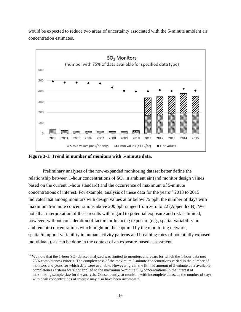
3-6
would be expected to reduce two areas of uncertainty associated with the 5-minute ambient air
concentration estimates.
Figure 3-1. Trend in number of monitors with 5-minute data.
Preliminary analyses of the now-expanded monitoring dataset better define the
relationship between 1-hour concentrations of SO2 in ambient air (and monitor design values
based on the current 1-hour standard) and the occurrence of maximum of 5-minute
concentrations of interest. For example, analysis of these data for the years28 2013 to 2015
indicates that among monitors with design values at or below 75 ppb, the number of days with
maximum 5-minute concentrations above 200 ppb ranged from zero to 22 (Appendix B). We
note that interpretation of these results with regard to potential exposure and risk is limited,
however, without consideration of factors influencing exposure (e.g., spatial variability in
ambient air concentrations which might not be captured by the monitoring network,
spatial/temporal variability in human activity patterns and breathing rates of potentially exposed
individuals), as can be done in the context of an exposure-based assessment.
28 We note that the 1-hour SO2 dataset analyzed was limited to monitors and years for which the 1-hour data met
75% completeness criteria. The completeness of the maximum 5-minute concentrations varied in the number of
monitors and years for which data were available. However, given the limited amount of 5-minute data available,
completeness criteria were not applied to the maximum 5-minute SO2 concentrations in the interest of
maximizing sample size for the analysis. Consequently, at monitors with incomplete datasets, the number of days
with peak concentrations of interest may also have been incomplete.
3-7
3.3.2 Characterizing the Spatial and Temporal Distribution of 1-hour SO2 Concentrations
The exposure-based assessment in the 2009 SO2 REA relied on air quality modeling
using the air dispersion model, AERMOD, to estimate 1-hour concentrations across each study
area over the years assessed for each air quality scenario. The current information continues to
support the use of an air dispersion model such as AERMOD over the use of other models, such
as photochemical models, for modeling of directly emitted SO2 concentrations for use in
assessing risk and exposure for this pollutant. Unlike dispersion models, photochemical models
cannot capture the sharp concentration gradients that can occur near SO2 sources. Also, SO2
emissions to ambient air are dominated by point sources, such as large coal-fired utilities, and
AERMOD is the EPA’s preferred air quality model for SO2 for State Implementation Plans
(SIPs) 29 and new source permitting purposes. For all of these reasons, AERMOD remains the
most appropriate model for predicting SO2 concentrations in ambient air.
Since the last review, there have been a number of changes to the AERMOD modeling
system which includes the AERMOD dispersion model itself, and associated data processors,
including the AERMET meteorological preprocessor, and the AERMAP terrain processor.
Specifically, there have been ten updates to the AERMOD model, six updates to AERMET, and
one update to AERMAP (U.S. EPA, 2016). There has also been the development of
AERMINUTE, a preprocessor to AERMET that calculates hourly average winds from 1-minute
ASOS winds at NWS stations (U.S. EPA, 2015). Some of these model changes are considered
major improvements and, in some instances, could significantly affect results (e.g., use of hourly
averaged winds from AERMINUTE, options for treatment of low wind situations, and treatment
of building downwash for stacks exceeding Good Engineering Practice (GEP) stack heights,
among others). How they might affect the results will vary depending on the particular feature.
For example, model changes could lead to increased concentrations at the upper percentiles of
the concentration distribution (such as use of AERMINUTE or treatment of building downwash
for stacks exceeding GEP). In other instances, the model changes, such as options for treatment
of low wind speeds (adjusted surface friction velocity) could lead to a decrease in concentrations
at the higher end of the concentration distribution.
3.4 EXPOSURE ESTIMATES
Exposure considerations are another essential component in the characterization of
exposure and risk associated with SO2 in ambient air. Such considerations include the factors
that affect exposures that are not addressed by consideration of ambient air concentrations as a
29 With regard to such plans, the Clean Air Act requires states to develop a general infrastructure plan to provide for
attainment and maintenance the NAAQS in all areas of the country, and a specific plan to provide for attainment
of the NAAQS for any area that has been designated as nonattainment for a NAAQS.
3-8
surrogate for exposure to SO2 from ambient air. In addition to the attenuation in SO2
concentrations expected to occur in microenvironments and the influence of human activity
patterns on exposure concentration, accounting for human physiology and the occurrence of
elevated ventilation rates concurrent with SO2 exposures is key to characterizing health risk for
SO2. This section focuses on areas of key uncertainty and limitations in the exposure assessment
for the 2009 REA for which there is newly available information, tools or approaches, and
considers the extent to which there is new information that might be expected to improve our
estimation of SO2 population exposure.
3.4.1 Microenvironmental Concentrations
In the 2009 REA, outdoor microenvironments were identified as contributing appreciably
to individual exposure concentrations, and the key area of uncertainty contributing to
concentrations for those microenvironments was uncertainty in the ambient air 5-minute
concentration estimates. As discussed in section 3.3 above, recent AERMOD improvements
might be expected to reduce uncertainty in estimates of 1-hour concentrations across the study
area that can vary spatially and temporally. Further, a substantially larger dataset of ambient air
measurements is now available that can be used to estimate 5-minute concentrations from 1-hour
modeling estimates, for all 12-hour 5-minute periods within each hour (section 3.3.1).
Accordingly, reduced uncertainty in estimates of 5-minute ambient air concentrations would be
expected to reduce uncertainty in microenvironmental concentrations for both outdoor and
indoor microenvironments.
3.4.2 Human Activity Patterns
The time-activity pattern data in CHAD is the basis for the activity sequences simulated
by APEX for each modeled individual, including simulation of time spent in different
microenvironments, a key influence on individuals’ exposure estimates. The CHAD has been
significantly updated since its use in the 2009 REA. The database used in the 2009 REA had
over 26,000 diaries (including about 12,000 for school-aged children ages 0-18). The CHAD
now has over 41,000 diaries, with over 13,000 for school-aged children (U.S. EPA, 2014a). Most
of the additional diaries come from more recent studies (2002-2014). This update could reduce
the uncertainty in the exposure and associated risk estimates for study populations, including
children with asthma.30
30 Although there are some CHAD diaries from persons who have asthma, most do not specify whether or not the
individual had asthma. Analyses of the CHAD data that were performed in both the 2009 SO2 REA (section
8.11.2.2) and the 2014 O3 REA (U.S EPA 2014b, section 5G-1.4) combined with related findings reported in the
extant literature (e.g., van Gent et al. 2007) indicate there is no appreciable difference in the time spent outdoors
3-9
3.4.3 Physical Attributes and Ventilation Rate
New information is available in this review for three other inputs to the exposure model.
This includes updated NHANES data (2009-2014), which are the basis for the age- and sex-
specific body mass distributions from which APEX samples to specify the individuals in the
modeled populations. In the uncertainty characterization for the 2009 REA, it was concluded that
uncertainty in these data would not affect the exposure estimates in any particular direction and
that because random sampling is used, it was expected that the magnitude of influence from this
source of uncertainty on exposure estimates would be low (2009 REA, section 8.11.2.2.3).
The other two items considered here are the algorithms used to estimate age-and sex-
specific resting metabolic rate (RMR), a key input to estimating a simulated individual’s activity
specific ventilation rate (V̇E), and the V̇E algorithm itself. Since the last review, we have been
reviewing the literature and evaluating potential updates to the RMR and V̇E algorithms used in
the version of APEX run for the 2009 REA (U.S. EPA, 2008a,b; U.S. EPA, 2009).
With regard to RMR, we have been reviewing the more recent literature and other
published sources containing individual data and compiling the associated individual RMR
measurements (over 16,000), along with associated influential attributes such as age, sex, and
body mass. This comprehensive, diverse collection of data from individuals is being used to
develop a new algorithm to replace that used by the version of APEX used for the 2009 REA
(version 4.3). That version of APEX used an algorithm for RMR originally based on analyses by
Schofield (1985).
With regard to V̇E, new individual measurement data were not found to update the V̇E
database on which the algorithm in the version of APEX used for 2009 REA is based.
However, a reanalysis has been performed based on revised assumptions regarding identification
of highly influential data points, and with consideration of an additional database variable. This
reanalysis is allowing for development of an updated algorithm that utilizes a greater number of
samples.
Additional details regarding the RMR and V̇E data used, algorithm development, and
performance evaluation will be available with APEX update, expected in spring 2017. Although
each of these expected updates represent improvements to the exposure modeling and reduce
uncertainty, the extent to which they might affect resultant estimates is unclear. Note also, the
inclusion of these updated data sets and algorithms into the APEX model will be dependent on
whether updated model is available as projected in accordance with the current review schedule.
or exertion levels for individuals with or without asthma. Accordingly, asthma status is not an attribute used in
sampling CHAD.
3-10
3.4.4 Exposure Estimate Bins
Specific aspects of the approach to binning the estimated exposures to which the E-R
functions were applied to estimate risk were recognized to contribute uncertainty to the lung
function risk estimates (75 FR 35520, June 22, 2010). For example, the size of the exposure bins
carries a certain level of precision, which for exposures generally distributed across a broad
range of exposures levels may be acceptable. However, in scenarios assessed in the 2009 REA
for air quality conditions associated with potential alternative standards near the existing 1-hour
standard, a substantial portion of the exposures fell into very few bins (at the lower end of the
range). Thus, for purposes of considering exposures for the existing standard, a greater precision
would be desirable particularly at the lowest exposure concentrations. This could be achieved
and the uncertainty and any bias contributed by bin size to the risk estimates could be addressed
by using smaller-sized bins (e.g., 10 ppb) to represent the exposure estimates.
3.5 CONCLUSIONS
The discussion above reflects the EPA staff assessment of the degree to which currently
available information, including that newly available since the last review (e.g., as summarized
in the second draft ISA), might be expected to appreciably change our understanding of
exposures and risk beyond the insights gained from the assessments from the last review. A
critical consideration is the extent to which use of newly available information or approaches in a
new or updated quantitative assessment would provide risk estimates for exposure to SO2 from
ambient air that are appreciably different or with which the uncertainty is substantially lower
than the estimates generated for the last review. Thus, the decision on whether to develop a
comprehensive new assessment of exposure and risk for this review considers the extent to
which our characterization of exposure and risk in the last review may remain appropriately
informative to the key questions in the current review. Accordingly, it also focuses on the extent
to which the newly available information, if applied to aspects of the exposure and risk approach
from the last review, has the potential to result in new exposure and risk estimates for which the
degree of uncertainty is substantially reduced, or bias is addressed, and that indicates that a new
assessment of exposure and risk is warranted to provide an adequate characterization of human
exposure and risk, particularly with regard to the existing standard.31
Key observations regarding the potential impact of newly available information,
particularly focusing on those influencing staff conclusions, are presented here in the general
order in which sources of uncertainty are considered in the previous sections.
31 In considering this point, the EPA staff additionally recognize that such a characterization of exposure and risk, in
addition to the currently available evidence, will be considered in the Policy Assessment in terms of both
evidence-based considerations and risk/exposure-based considerations.
3-11
SO2 Air Concentrations: There are substantially more 5-minute SO2 monitoring data
available across many more monitors, both hourly maximum 5-minute concentrations
and the full series of 5-minute concentrations for each hour, thus providing a substantially
improved foundation for estimating 5-minute exposure concentrations that reflect recent
information. These new data, in conjunction with improvements to AERMOD since the
last review, would also be expected to reduce uncertainties associated with estimating
SO2 concentrations in ambient air across a geographical area. Together this updated
information would be expected to substantially improve our characterization of 5-minute
SO2 concentrations in ambient air.
Exposure Assessment: As recognized in section 3.3 above, exposure modeling can be
particularly informative to our understanding of the potential for SO2 concentrations in
ambient air to contribute to exposures of concern for at-risk populations (e.g., individuals
with asthma while at elevated ventilation rates). A greatly expanded database of activity
diaries (CHAD) may be expected to provide a stronger foundation for exposure
modeling. In addition, reduced uncertainty in ambient air 5-minute concentration
estimates (per above bullet) would be expected to reduce uncertainty in the
microenvironment concentrations, including for outdoor microenvironments, which
substantially influence peak exposure estimates. Together, this updated information
would be expected to contribute to somewhat reduced uncertainty in the exposure
estimates.
Risk Characterization: Although little new information is available in this review to
characterize lung function response to SO2 exposures, several steps could be taken to
improve upon the lung-function risk model applied in the 2009 REA. Expansion of the
dataset that is used to derive lung function E-R functions may reduce uncertainty in the
shape of the functions across the study data range. Smaller exposure estimate bins would
increase the precision of risk estimates, by better linking estimated exposures with the
lung function E-R relationship. Further, sensitivity analyses for the E-R function
application to exposures below those studied would augment our characterization of the
associated uncertainty contributing to a more robust characterization of lung function risk
in the range of the study data and of uncertainties at lower exposures.
With regard to the conceptual model for exposure and health risk, we conclude that the
newly available information does not appreciably change key aspects of the conceptual model
from the last review. The important new information summarized above would, however,
contribute to updated and less uncertain inputs for some aspects of the model (e.g., particularly
characterization of 5-minute concentrations), with the potential to be appreciably different from
the last review. Such reduction in uncertainty is key aspects of the model would be expected to
improve the robustness of the exposure and risk estimates over those from the last review.
We additionally recognize that the 2009 REA did not include an air quality scenario for
the current standard of 75 ppb; rather, we relied on inferences drawn from estimates for the air
quality scenarios for standard levels bounding the standard (i.e., either just meeting a 50 ppb or
100 ppb standard level). This was the case considering results from both the exposure-based
assessment and the air quality-based assessment. The former assessment was essential to our
3-12
complete characterization of SO2-related exposure and associated risk because the air quality-
based assessment could not take into account factors that significantly influence actual SO2
exposures and associated risk, including the movement of individuals through different
microenvironments and across large geographic areas all while also at varying breathing rates.
Accordingly, in order to adequately consider the exposure/risk implications of the substantially
expanded air quality dataset, the exposure modeling-based approach is essential.
In summary, a decision to utilize the new information and approaches summarized above
to develop a new REA that provides a more precise characterization of exposure and risk
associated with the existing standard, and one with reduced uncertainty, would provide
exposure/risk estimates with enhanced utility for informing the current review. Therefore, we
conclude that it is appropriate to consider development of an exposure and risk assessment,
based on this now available information and methods, to inform the current review of the
primary SO2 standard. Proposed plans for such an assessment are described in chapter 4.
3-13
REFERENCES
Alhanti BA, Chang HH, Winquist A, Mulholland JA, Darrow LA, Sarnat SE. 2016. Ambient air
pollution and emergency department visits for asthma: A multi-city assessment of effect
modification by age. J Expo Sci Environ Epidemiol. 26:180-188.
Byers N, Ritchey M, Vaidyanathan A, Brandt AJ, Yip F. 2016. Short-term effects of ambient air
pollutants on asthma-related emergency department visits in Indianapolis, Indiana, 2007-
2011. J Asthma. 53:245-252.
Horstman D, Roger LJ, Kehrl H, Hazucha M. 1986. Airway sensitivity of asthmatics to sulfur
dioxide. Toxicol Ind Health 2:289-298.
Li S, Batterman S, Wasilevich E, Wahl R, Wirth J, Su FC, et al. 2011. Association of daily
asthma emergency department visits and hospital admissions with ambient air pollutants
among the pediatric medicaid population in Detroit: Time-series and time-stratified case-
crossover analyses with threshold effects. Environ Res. 111:1137-1147.
Linn W, Venet T, Shamoo D, Valencia L, Anzar U, Spier C, Hackney J. 1983. Respiratory
effects of sulfur dioxide in heavily exercising asthmatics: a dose-response study.
American Review of Respiratory Disease 127:278-283.
Schofield WN. 1985. Predicting basal metabolic rate, new standards, and review of previous
work. Hum Nutr Clin Nutr. 39C(S1):5-41.
Strickland MJ, Darrow LA, Klein M, Flanders WD, Sarnat JA, Waller LA, et al. 2010. Short-
term associations between ambient air pollutants and pediatric asthma emergency
department visits. Am J Respir Crit Care Med. 182:307-316.
U.S. EPA. 2008a. Total Risk Integrated Methodology (TRIM) - Air Pollutants Exposure Model
Documentation (TRIM.Expo / APEX, Version 4.3) Volume I: User’s Guide. Office of
Air Quality Planning and Standards, Research Triangle Park, NC. January 2009.
Available at: https://www.epa.gov/fera/apex-user-guides
U.S. EPA. 2008b. Total Risk Integrated Methodology (TRIM) - Air Pollutants Exposure Model
Documentation (TRIM.Expo / APEX, Version 4.3) Volume II: Technical Support
Document. Office of Air Quality Planning and Standards, Research Triangle Park, NC.
January 2009. Available at: https://www.epa.gov/fera/apex-user-guides
U.S. EPA. 2009. APEX, verson 4.3. Available at: https://www.epa.gov/fera/download-trimexpo-
inhalation-apex
U.S. EPA. 2014a. The Consolidated Human Activity Database – Master Version (CHAD-
Master). Technical Memorandum. U.S. Environmental Protection Agency, National
Exposure Research Laboratory, Research Triangle Park, NC, 27711. Updated
09/15/2014. Available at: https://www.epa.gov/healthresearch/consolidated-human-
activity-database-chad-use-human-exposure-and-health-studies-and\

3-14
U.S. EPA. 2014b. Health Risk and Exposure Assessment for Ozone. Office of Air Quality
Planning and Standards, U.S. Environmental Protection Agency, Research Triangle Park,
NC, 27711. EPA-452/R-14-004a. Available at: https://www.epa.gov/naaqs/ozone-o3-
standards-risk-and-exposure-assessments-current-review
U.S EPA. 2015. AERMINUTE User’s Guide. EPA-454/B-15-006. U.S. Environmental
Protection Agency, Research Triangle Park, North Carolina 27711.
U.S. EPA. 2016. User's Guide for the AERMOD Terrain Preprocessor (AERMAP). EPA-454/B-
16-012. U.S. Environmental Protection Agency, Research Triangle Park, North Carolina
27711.
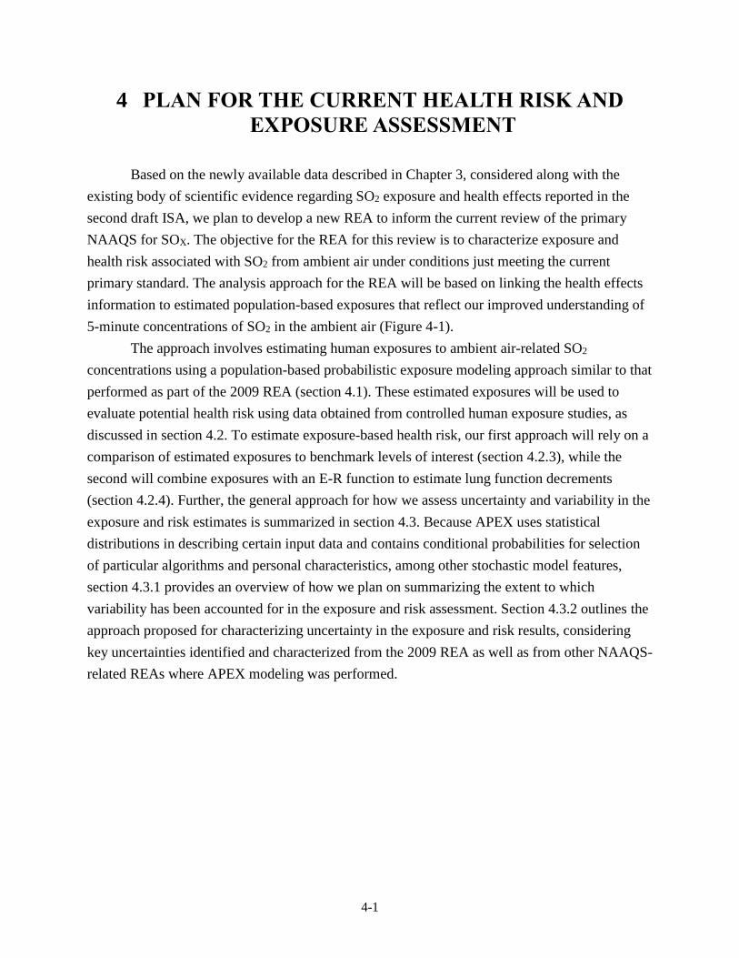
4-1
4 PLAN FOR THE CURRENT HEALTH RISK AND
EXPOSURE ASSESSMENT
Based on the newly available data described in Chapter 3, considered along with the
existing body of scientific evidence regarding SO2 exposure and health effects reported in the
second draft ISA, we plan to develop a new REA to inform the current review of the primary
NAAQS for SOX. The objective for the REA for this review is to characterize exposure and
health risk associated with SO2 from ambient air under conditions just meeting the current
primary standard. The analysis approach for the REA will be based on linking the health effects
information to estimated population-based exposures that reflect our improved understanding of
5-minute concentrations of SO2 in the ambient air (Figure 4-1).
The approach involves estimating human exposures to ambient air-related SO2
concentrations using a population-based probabilistic exposure modeling approach similar to that
performed as part of the 2009 REA (section 4.1). These estimated exposures will be used to
evaluate potential health risk using data obtained from controlled human exposure studies, as
discussed in section 4.2. To estimate exposure-based health risk, our first approach will rely on a
comparison of estimated exposures to benchmark levels of interest (section 4.2.3), while the
second will combine exposures with an E-R function to estimate lung function decrements
(section 4.2.4). Further, the general approach for how we assess uncertainty and variability in the
exposure and risk estimates is summarized in section 4.3. Because APEX uses statistical
distributions in describing certain input data and contains conditional probabilities for selection
of particular algorithms and personal characteristics, among other stochastic model features,
section 4.3.1 provides an overview of how we plan on summarizing the extent to which
variability has been accounted for in the exposure and risk assessment. Section 4.3.2 outlines the
approach proposed for characterizing uncertainty in the exposure and risk results, considering
key uncertainties identified and characterized from the 2009 REA as well as from other NAAQS-
related REAs where APEX modeling was performed.
4-2
Figure 4-1. Overview of the analysis approach for the REA.
4.1 POPULATION-BASED EXPOSURE ASSESSMENT
Population exposures to SO2 from ambient air will be estimated for at-risk populations in
selected study areas for air quality conditions associated with just meeting the existing primary
standard, as well as recent conditions.32 Exposures will be estimated using the most recent
version of the APEX model available.33 Details regarding the modeling approach, the input data
32 The need for additional air quality scenarios (if any) will be considered in the draft PA that will accompany the
draft REA presenting results for the analyses described here.
33 Earlier versions of APEX have been used to estimate population exposures to O3, carbon monoxide, NO2 and SO2
in previous NAAQS reviews (U.S. EPA, 2014b, 2010, 2008; 2009 REA) to better inform our understanding of
how variability in ambient air pollutant concentrations and other influential attributes relate to human exposure.
An APEX model update is expected to be available in spring 2017. The model, associated updated input
databases and user’s guide will be available at: https://www.epa.gov/fera/human-exposure-modeling-air-
pollutants-exposure-model.
4-3
to be used, and model specifications for the population groups and study areas of interest are
provided in the subsections below.
Because controlled human exposure studies indicate exposures of interest are of short-
term duration (5 to 10 minutes), estimated 5-minute average exposures will be the focus in the
design of the assessment and in evaluating potential health risk. Potential health risk associated
with air quality adjusted to just meet the existing SO2 standard (and recent unadjusted air quality)
will be characterized using two different metrics: (1) the number and percent of the simulated
study area population experiencing 5-minute SO2 exposures at or above benchmark levels of
concern (section 4.2.1) and (2) the number of occurrences of lung function decrements (based on
predicted occurrence of sRaw increases above 100% and above 200%) in the simulated at-risk
populations and the number and percent of the simulated at-risk populations estimated to
experience single or multiple occurrences of those lung function decrements (section 4.2.2).
Additionally, as part of this analysis, the population-based statistical distribution of exposures
will also be evaluated to identify important exposure environments and/or influential activities
that lead to those estimated as having greatest potential health risk.
4.1.1 APEX Model Overview
As summarized in section 2.3.2, APEX is a model used to simulate a large number of
individuals within a selected study area, that are randomly sampled using a probabilistic
approach to reflect the area’s population demographics, thus generating study area-wide
estimates of population exposure. Any number of simulated individuals can be modeled by
APEX, and collectively they represent a random sample of the study area population in the
modeled area. Very broadly, APEX stochastically combines information from several large input
databases including, but not limited to, the 2010 U.S. Census (e.g., population demographics,
home-to-work commuting flows), U.S. EPA’s CHAD (e.g., human time-location-daily activity
patterns), and temporally-spatially distinct ambient air concentrations. Using these data and
several other sources of information, APEX simulates human exposures that occur in user-
defined indoor, outdoor, and in-vehicle microenvironments (MEs). Because APEX is capable of
using input data at fine temporal (e.g., 5-minute SO2 concentrations, minute-by-minute human
activity patterns) and spatial scales (e.g., census tract SO2 concentrations) and simulates
individuals within a population, the estimated exposures can be output as a time-series of
exposures for each and any individual or aggregated to population-based summary exposure
metrics of interest. Further details about APEX can be found in the existing Users’ Guide and
Technical Support Document (U.S. EPA, 2012a, b).
4-4
4.1.2 Exposure Domain
The exposure domain is defined by the exposure assessment features of interest, i.e.,
broadly addressing the questions of where, when, and for whom the assessment pertains.
Answers to these questions are informed by the scientific evidence regarding SO2 exposures and
associated health risks, the availability and analysis of the SO2 concentrations in ambient air at
the relevant time scale, reasonableness of technical capabilities (e.g., approach availability and
appropriateness), and risk metrics to be generated.
4.1.2.1 Study Areas and Time Periods
We plan to build on the exposure and risk assessments conducted for the last review and
continue to focus the assessments on a set of selected study areas. In the 2009 REA, two study
areas were evaluated, with each having exposures estimated for a single year. For this REA, we
intend to assess exposures in a small number of study areas, each modeled for three consecutive
years to evaluate variability in exposures across a 3-year period, consistent with the form of the
existing standard.
In considering the available monitoring data with regard to its use in planning and/or
performing a REA, we first consider the distribution of monitors in areas across the U.S. and the
extent to which a potential study area may be appropriately represented by a single monitor (a
single monitor near a specific emission source) or multiple monitors within the study area (e.g.,
numerous monitors in an urban area). To this end, before developing selection criteria and
identifying candidate study areas of interest for modeling exposure and health risk in this REA,
we considered the overall local-scale density of the SO2 monitoring network and developed an
approach to define both aggregate and single monitor areas. We first grouped any SO2 monitors
reporting both 1-hour and 5-minute maximum concentrations that were within 10 km of each
other, effectively forming a group. Monitors that were not within 10 km of another monitor were
considered alone; these single monitor areas represented more than 90% of the SO2 monitors
considered. Using these groupings, we then considered the following factors in the selection of
study areas and specific time periods using the following three criteria:
Air quality data: The time period of interest is 2011-2015, because 2011 was the first
year having greatly expanded numbers of ambient air monitors reporting 5-minute
concentrations and 2015 is the most recent year available to date during the development
of this REA Planning Document.34 A candidate study area needed to have SO2 ambient
air monitoring data that met completeness requirements (section 4.1.4.1) for a recent
three-year period, for all three years. This requirement is necessary to calculate design
34 If 2016 data become available and are in accordance with the REA schedule, they would be included in the study
area selection for the REA.
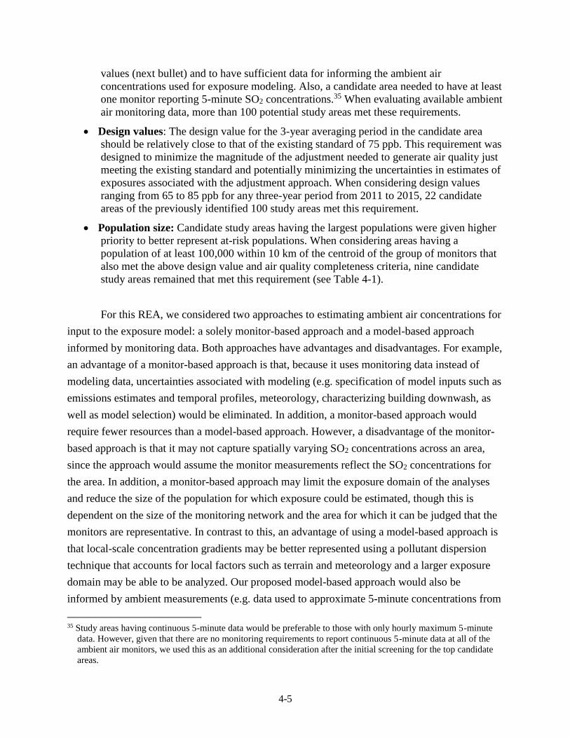
4-5
values (next bullet) and to have sufficient data for informing the ambient air
concentrations used for exposure modeling. Also, a candidate area needed to have at least
one monitor reporting 5-minute SO2 concentrations.35 When evaluating available ambient
air monitoring data, more than 100 potential study areas met these requirements.
Design values: The design value for the 3-year averaging period in the candidate area
should be relatively close to that of the existing standard of 75 ppb. This requirement was
designed to minimize the magnitude of the adjustment needed to generate air quality just
meeting the existing standard and potentially minimizing the uncertainties in estimates of
exposures associated with the adjustment approach. When considering design values
ranging from 65 to 85 ppb for any three-year period from 2011 to 2015, 22 candidate
areas of the previously identified 100 study areas met this requirement.
Population size: Candidate study areas having the largest populations were given higher
priority to better represent at-risk populations. When considering areas having a
population of at least 100,000 within 10 km of the centroid of the group of monitors that
also met the above design value and air quality completeness criteria, nine candidate
study areas remained that met this requirement (see Table 4-1).
For this REA, we considered two approaches to estimating ambient air concentrations for
input to the exposure model: a solely monitor-based approach and a model-based approach
informed by monitoring data. Both approaches have advantages and disadvantages. For example,
an advantage of a monitor-based approach is that, because it uses monitoring data instead of
modeling data, uncertainties associated with modeling (e.g. specification of model inputs such as
emissions estimates and temporal profiles, meteorology, characterizing building downwash, as
well as model selection) would be eliminated. In addition, a monitor-based approach would
require fewer resources than a model-based approach. However, a disadvantage of the monitor-
based approach is that it may not capture spatially varying SO2 concentrations across an area,
since the approach would assume the monitor measurements reflect the SO2 concentrations for
the area. In addition, a monitor-based approach may limit the exposure domain of the analyses
and reduce the size of the population for which exposure could be estimated, though this is
dependent on the size of the monitoring network and the area for which it can be judged that the
monitors are representative. In contrast to this, an advantage of using a model-based approach is
that local-scale concentration gradients may be better represented using a pollutant dispersion
technique that accounts for local factors such as terrain and meteorology and a larger exposure
domain may be able to be analyzed. Our proposed model-based approach would also be
informed by ambient measurements (e.g. data used to approximate 5-minute concentrations from
35 Study areas having continuous 5-minute data would be preferable to those with only hourly maximum 5-minute
data. However, given that there are no monitoring requirements to report continuous 5-minute data at all of the
ambient air monitors, we used this as an additional consideration after the initial screening for the top candidate
areas.
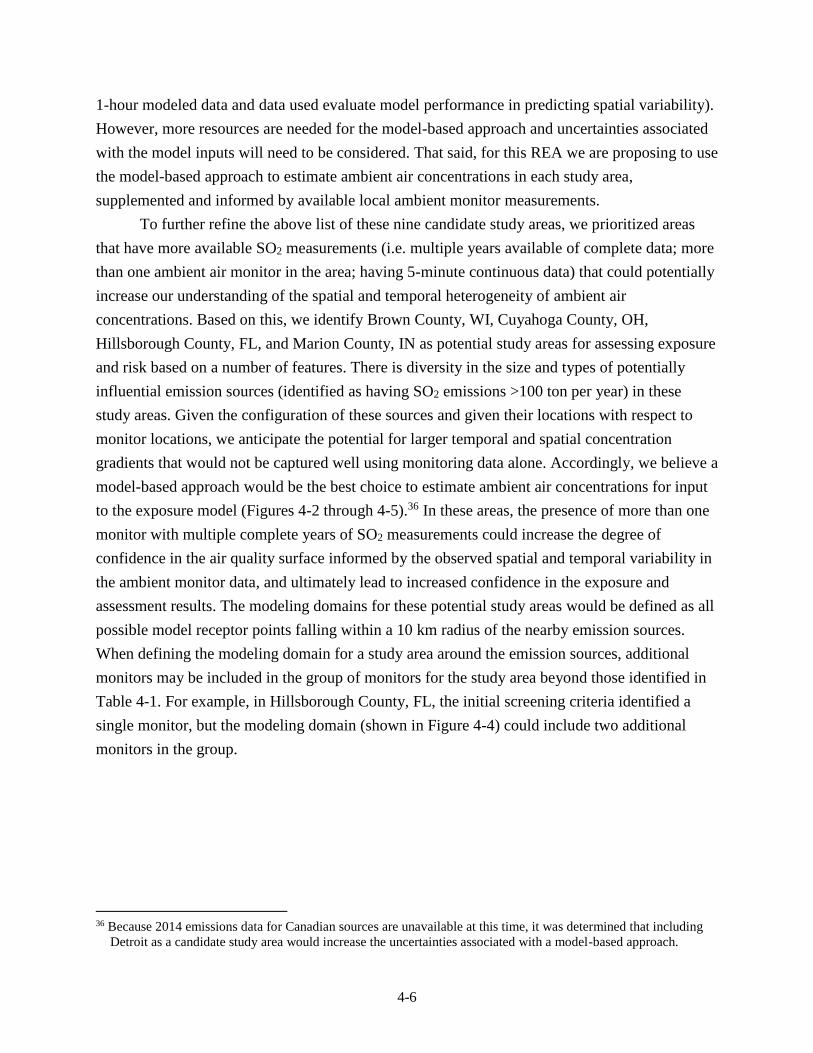
4-6
1-hour modeled data and data used evaluate model performance in predicting spatial variability).
However, more resources are needed for the model-based approach and uncertainties associated
with the model inputs will need to be considered. That said, for this REA we are proposing to use
the model-based approach to estimate ambient air concentrations in each study area,
supplemented and informed by available local ambient monitor measurements.
To further refine the above list of these nine candidate study areas, we prioritized areas
that have more available SO2 measurements (i.e. multiple years available of complete data; more
than one ambient air monitor in the area; having 5-minute continuous data) that could potentially
increase our understanding of the spatial and temporal heterogeneity of ambient air
concentrations. Based on this, we identify Brown County, WI, Cuyahoga County, OH,
Hillsborough County, FL, and Marion County, IN as potential study areas for assessing exposure
and risk based on a number of features. There is diversity in the size and types of potentially
influential emission sources (identified as having SO2 emissions >100 ton per year) in these
study areas. Given the configuration of these sources and given their locations with respect to
monitor locations, we anticipate the potential for larger temporal and spatial concentration
gradients that would not be captured well using monitoring data alone. Accordingly, we believe a
model-based approach would be the best choice to estimate ambient air concentrations for input
to the exposure model (Figures 4-2 through 4-5).36 In these areas, the presence of more than one
monitor with multiple complete years of SO2 measurements could increase the degree of
confidence in the air quality surface informed by the observed spatial and temporal variability in
the ambient monitor data, and ultimately lead to increased confidence in the exposure and
assessment results. The modeling domains for these potential study areas would be defined as all
possible model receptor points falling within a 10 km radius of the nearby emission sources.
When defining the modeling domain for a study area around the emission sources, additional
monitors may be included in the group of monitors for the study area beyond those identified in
Table 4-1. For example, in Hillsborough County, FL, the initial screening criteria identified a
single monitor, but the modeling domain (shown in Figure 4-4) could include two additional
monitors in the group.
36 Because 2014 emissions data for Canadian sources are unavailable at this time, it was determined that including
Detroit as a candidate study area would increase the uncertainties associated with a model-based approach.
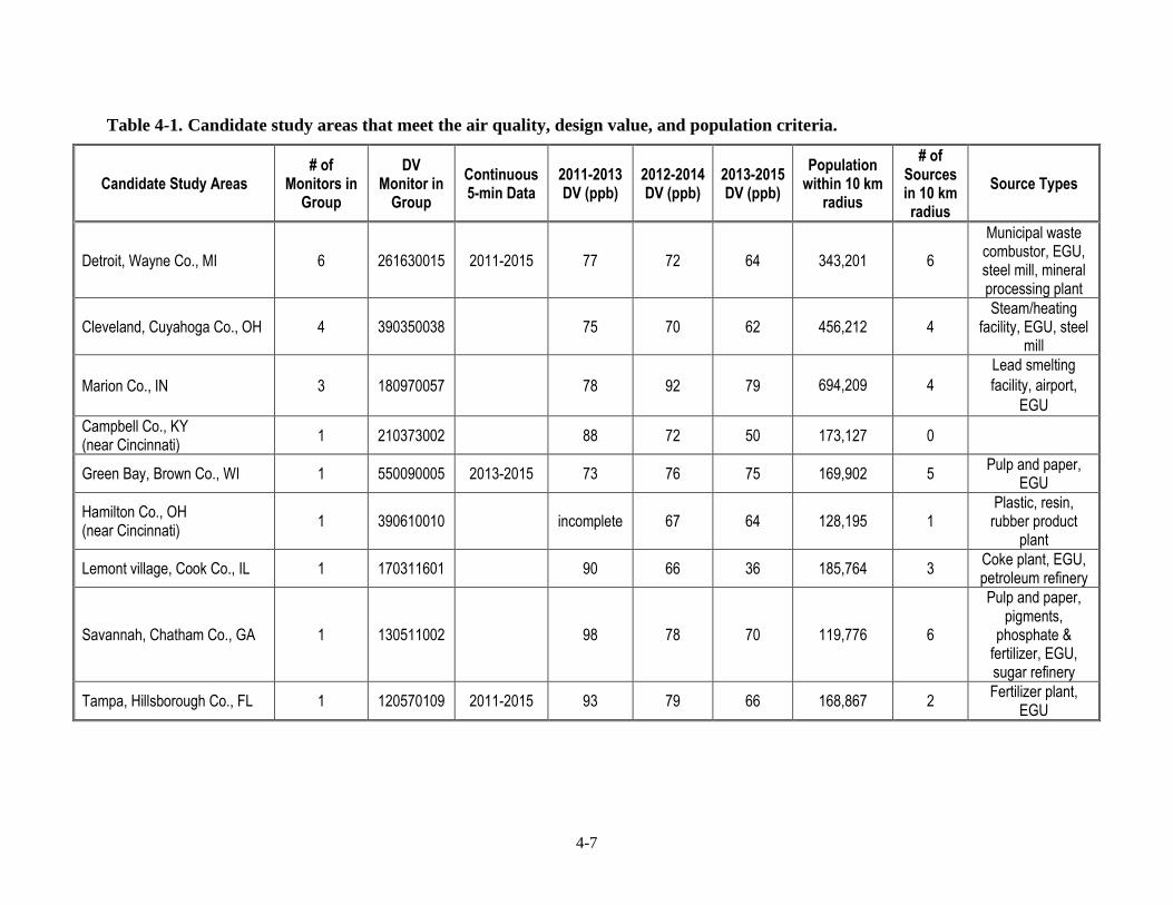
4-7
Table 4-1. Candidate study areas that meet the air quality, design value, and population criteria.
Candidate Study Areas # of
Monitors in Group
DV Monitor in
Group
Continuous 5-min Data
2011-2013 DV (ppb)
2012-2014 DV (ppb)
2013-2015 DV (ppb)
Population within 10 km
radius
# of Sources in 10 km radius
Source Types
Detroit, Wayne Co., MI 6 261630015 2011-2015 77 72 64 343,201 6
Municipal waste combustor, EGU, steel mill, mineral processing plant
Cleveland, Cuyahoga Co., OH 4 390350038 75 70 62 456,212 4 Steam/heating
facility, EGU, steel mill
Marion Co., IN 3 180970057 78 92 79 694,209 4
Lead smelting
facility, airport,
EGU
Campbell Co., KY (near Cincinnati)
1 210373002 88 72 50 173,127 0
Green Bay, Brown Co., WI 1 550090005 2013-2015 73 76 75 169,902 5 Pulp and paper,
EGU
Hamilton Co., OH (near Cincinnati)
1 390610010 incomplete 67 64 128,195 1 Plastic, resin,
rubber product plant
Lemont village, Cook Co., IL 1 170311601 90 66 36 185,764 3 Coke plant, EGU, petroleum refinery
Savannah, Chatham Co., GA 1 130511002 98 78 70 119,776 6
Pulp and paper, pigments,
phosphate & fertilizer, EGU, sugar refinery
Tampa, Hillsborough Co., FL 1 120570109 2011-2015 93 79 66 168,867 2 Fertilizer plant,
EGU
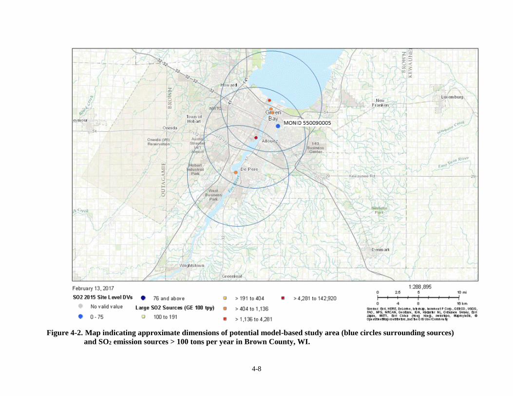
4-8
Figure 4-2. Map indicating approximate dimensions of potential model-based study area (blue circles surrounding sources)
and SO2 emission sources > 100 tons per year in Brown County, WI.
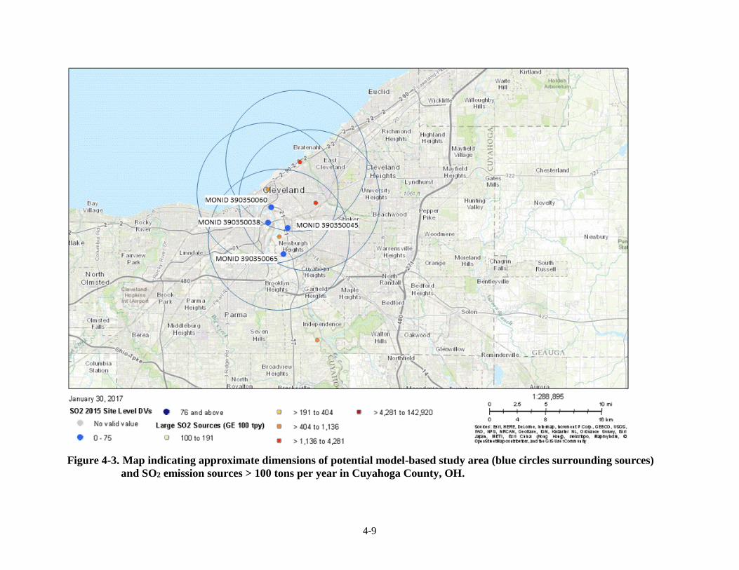
4-9
Figure 4-3. Map indicating approximate dimensions of potential model-based study area (blue circles surrounding sources)
and SO2 emission sources > 100 tons per year in Cuyahoga County, OH.
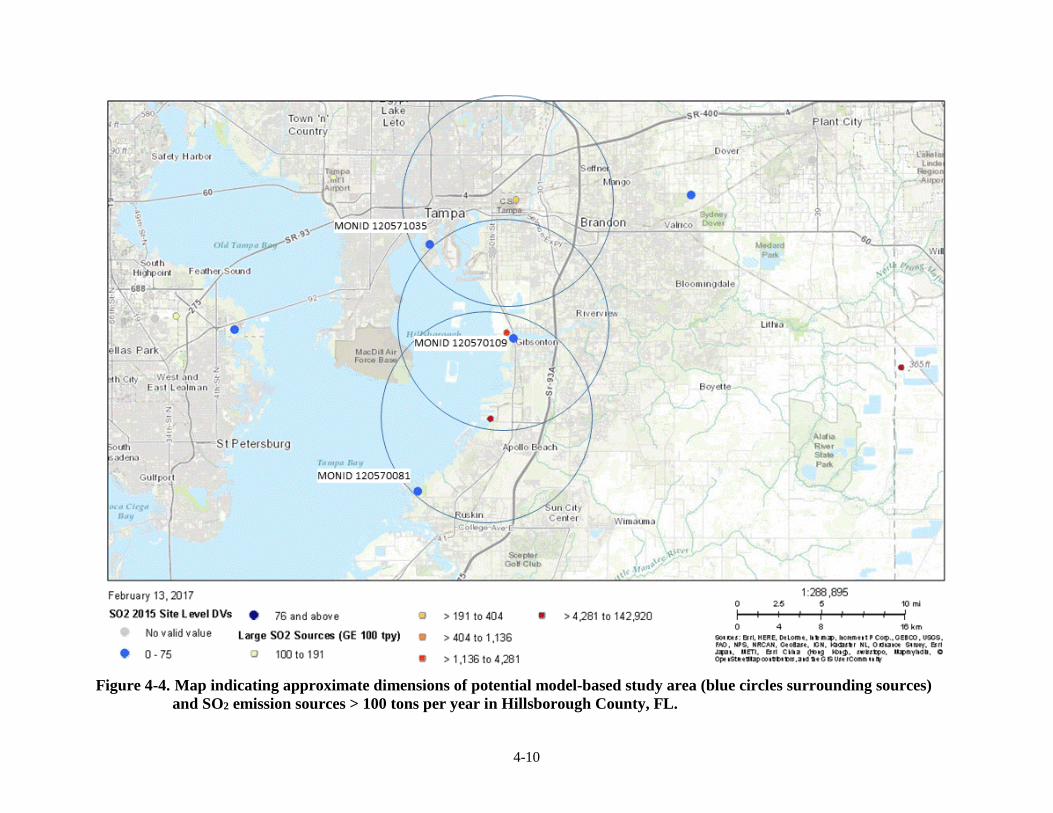
4-10
Figure 4-4. Map indicating approximate dimensions of potential model-based study area (blue circles surrounding sources)
and SO2 emission sources > 100 tons per year in Hillsborough County, FL.
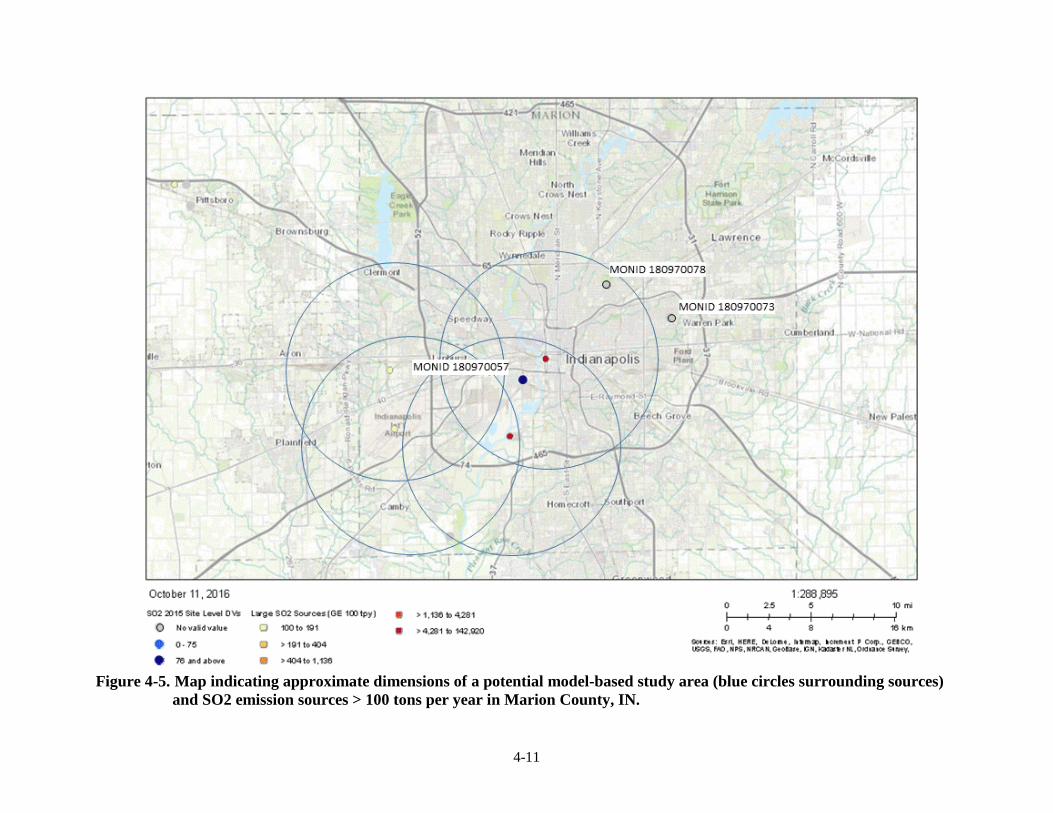
4-11
Figure 4-5. Map indicating approximate dimensions of a potential model-based study area (blue circles surrounding sources)
and SO2 emission sources > 100 tons per year in Marion County, IN.
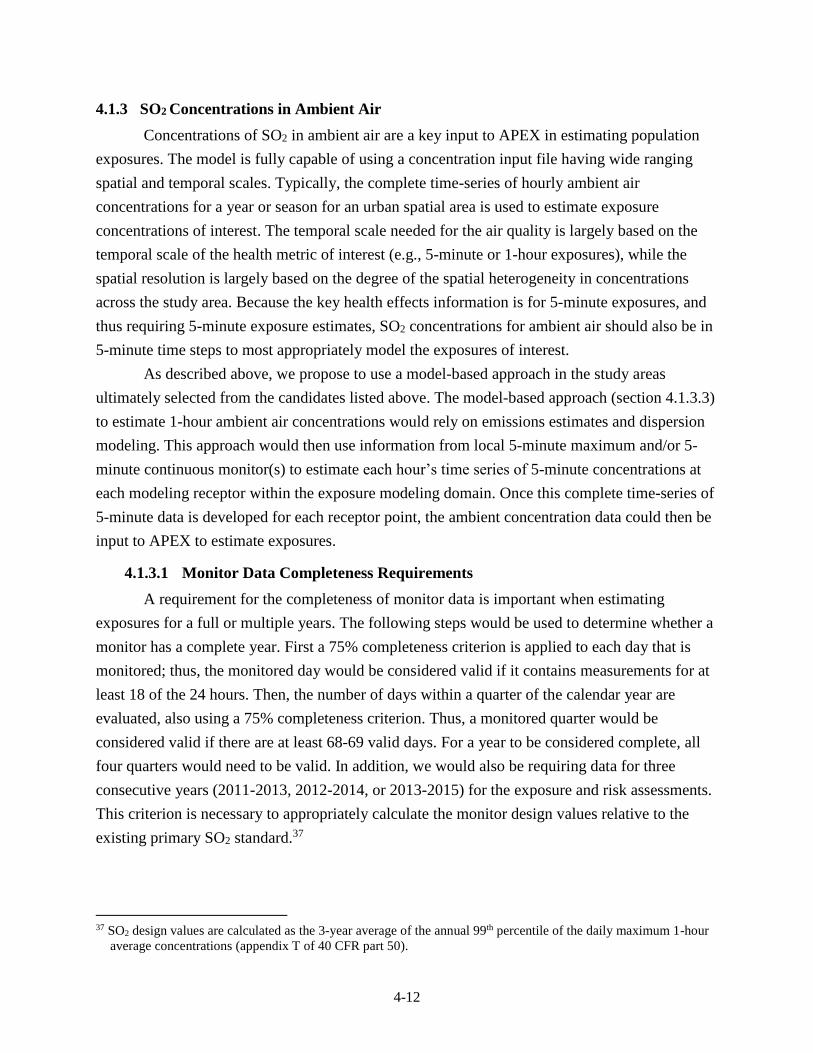
4-12
4.1.3 SO2 Concentrations in Ambient Air
Concentrations of SO2 in ambient air are a key input to APEX in estimating population
exposures. The model is fully capable of using a concentration input file having wide ranging
spatial and temporal scales. Typically, the complete time-series of hourly ambient air
concentrations for a year or season for an urban spatial area is used to estimate exposure
concentrations of interest. The temporal scale needed for the air quality is largely based on the
temporal scale of the health metric of interest (e.g., 5-minute or 1-hour exposures), while the
spatial resolution is largely based on the degree of the spatial heterogeneity in concentrations
across the study area. Because the key health effects information is for 5-minute exposures, and
thus requiring 5-minute exposure estimates, SO2 concentrations for ambient air should also be in
5-minute time steps to most appropriately model the exposures of interest.
As described above, we propose to use a model-based approach in the study areas
ultimately selected from the candidates listed above. The model-based approach (section 4.1.3.3)
to estimate 1-hour ambient air concentrations would rely on emissions estimates and dispersion
modeling. This approach would then use information from local 5-minute maximum and/or 5-
minute continuous monitor(s) to estimate each hour’s time series of 5-minute concentrations at
each modeling receptor within the exposure modeling domain. Once this complete time-series of
5-minute data is developed for each receptor point, the ambient concentration data could then be
input to APEX to estimate exposures.
4.1.3.1 Monitor Data Completeness Requirements
A requirement for the completeness of monitor data is important when estimating
exposures for a full or multiple years. The following steps would be used to determine whether a
monitor has a complete year. First a 75% completeness criterion is applied to each day that is
monitored; thus, the monitored day would be considered valid if it contains measurements for at
least 18 of the 24 hours. Then, the number of days within a quarter of the calendar year are
evaluated, also using a 75% completeness criterion. Thus, a monitored quarter would be
considered valid if there are at least 68-69 valid days. For a year to be considered complete, all
four quarters would need to be valid. In addition, we would also be requiring data for three
consecutive years (2011-2013, 2012-2014, or 2013-2015) for the exposure and risk assessments.
This criterion is necessary to appropriately calculate the monitor design values relative to the
existing primary SO2 standard.37
37 SO2 design values are calculated as the 3-year average of the annual 99th percentile of the daily maximum 1-hour
average concentrations (appendix T of 40 CFR part 50).
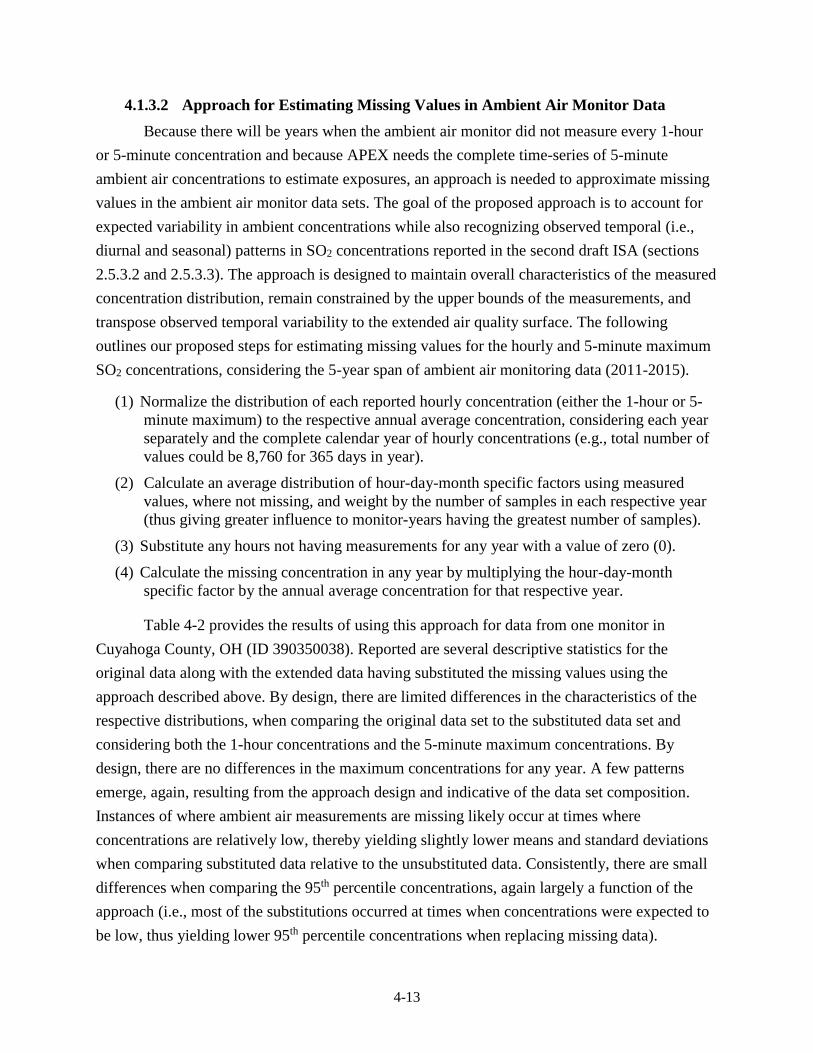
4-13
4.1.3.2 Approach for Estimating Missing Values in Ambient Air Monitor Data
Because there will be years when the ambient air monitor did not measure every 1-hour
or 5-minute concentration and because APEX needs the complete time-series of 5-minute
ambient air concentrations to estimate exposures, an approach is needed to approximate missing
values in the ambient air monitor data sets. The goal of the proposed approach is to account for
expected variability in ambient concentrations while also recognizing observed temporal (i.e.,
diurnal and seasonal) patterns in SO2 concentrations reported in the second draft ISA (sections
2.5.3.2 and 2.5.3.3). The approach is designed to maintain overall characteristics of the measured
concentration distribution, remain constrained by the upper bounds of the measurements, and
transpose observed temporal variability to the extended air quality surface. The following
outlines our proposed steps for estimating missing values for the hourly and 5-minute maximum
SO2 concentrations, considering the 5-year span of ambient air monitoring data (2011-2015).
(1) Normalize the distribution of each reported hourly concentration (either the 1-hour or 5-
minute maximum) to the respective annual average concentration, considering each year
separately and the complete calendar year of hourly concentrations (e.g., total number of
values could be 8,760 for 365 days in year).
(2) Calculate an average distribution of hour-day-month specific factors using measured
values, where not missing, and weight by the number of samples in each respective year
(thus giving greater influence to monitor-years having the greatest number of samples).
(3) Substitute any hours not having measurements for any year with a value of zero (0).
(4) Calculate the missing concentration in any year by multiplying the hour-day-month
specific factor by the annual average concentration for that respective year.
Table 4-2 provides the results of using this approach for data from one monitor in
Cuyahoga County, OH (ID 390350038). Reported are several descriptive statistics for the
original data along with the extended data having substituted the missing values using the
approach described above. By design, there are limited differences in the characteristics of the
respective distributions, when comparing the original data set to the substituted data set and
considering both the 1-hour concentrations and the 5-minute maximum concentrations. By
design, there are no differences in the maximum concentrations for any year. A few patterns
emerge, again, resulting from the approach design and indicative of the data set composition.
Instances of where ambient air measurements are missing likely occur at times where
concentrations are relatively low, thereby yielding slightly lower means and standard deviations
when comparing substituted data relative to the unsubstituted data. Consistently, there are small
differences when comparing the 95th percentile concentrations, again largely a function of the
approach (i.e., most of the substitutions occurred at times when concentrations were expected to
be low, thus yielding lower 95th percentile concentrations when replacing missing data).
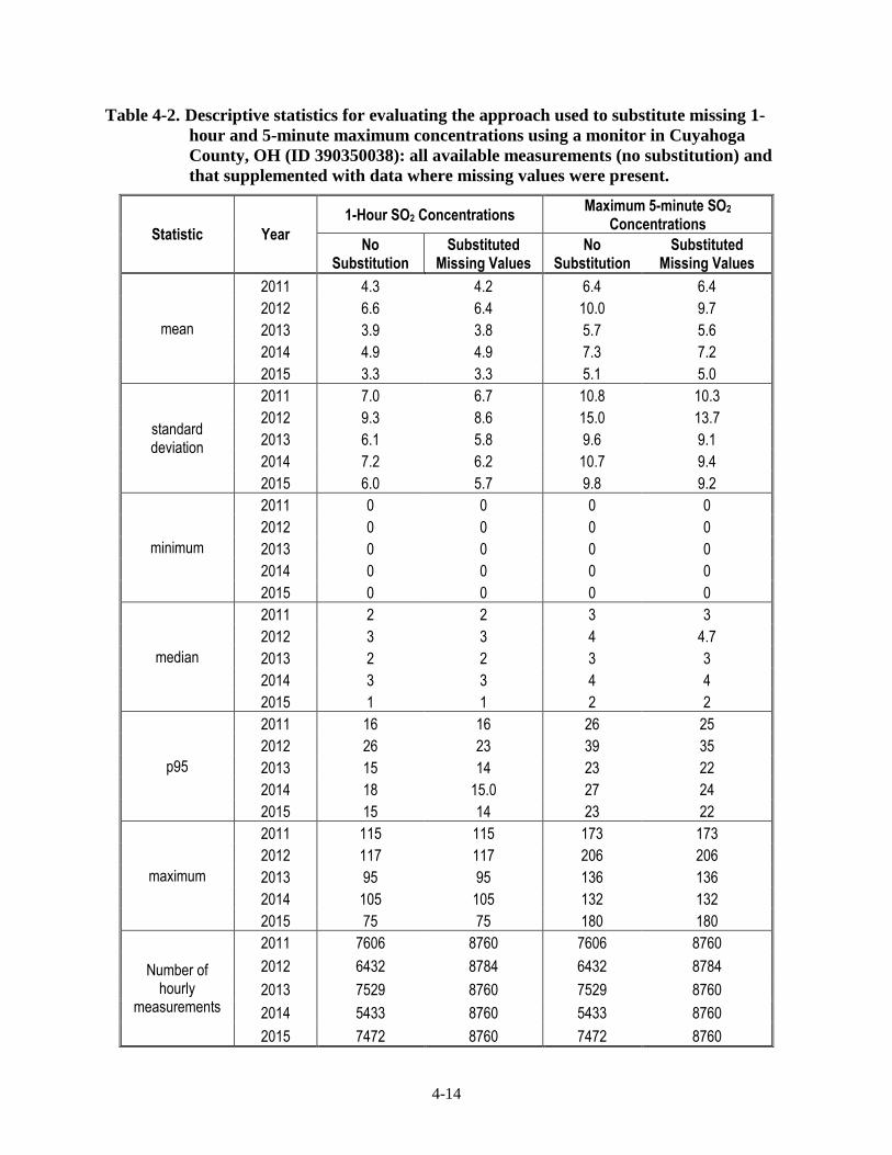
4-14
Table 4-2. Descriptive statistics for evaluating the approach used to substitute missing 1-
hour and 5-minute maximum concentrations using a monitor in Cuyahoga
County, OH (ID 390350038): all available measurements (no substitution) and
that supplemented with data where missing values were present.
Statistic Year
1-Hour SO2 Concentrations Maximum 5-minute SO2
Concentrations
No Substitution
Substituted Missing Values
No Substitution
Substituted Missing Values
mean
2011 4.3 4.2 6.4 6.4
2012 6.6 6.4 10.0 9.7
2013 3.9 3.8 5.7 5.6
2014 4.9 4.9 7.3 7.2
2015 3.3 3.3 5.1 5.0
standard deviation
2011 7.0 6.7 10.8 10.3
2012 9.3 8.6 15.0 13.7
2013 6.1 5.8 9.6 9.1
2014 7.2 6.2 10.7 9.4
2015 6.0 5.7 9.8 9.2
minimum
2011 0 0 0 0
2012 0 0 0 0
2013 0 0 0 0
2014 0 0 0 0
2015 0 0 0 0
median
2011 2 2 3 3
2012 3 3 4 4.7
2013 2 2 3 3
2014 3 3 4 4
2015 1 1 2 2
p95
2011 16 16 26 25
2012 26 23 39 35
2013 15 14 23 22
2014 18 15.0 27 24
2015 15 14 23 22
maximum
2011 115 115 173 173
2012 117 117 206 206
2013 95 95 136 136
2014 105 105 132 132
2015 75 75 180 180
Number of hourly
measurements
2011 7606 8760 7606 8760
2012 6432 8784 6432 8784
2013 7529 8760 7529 8760
2014 5433 8760 5433 8760
2015 7472 8760 7472 8760
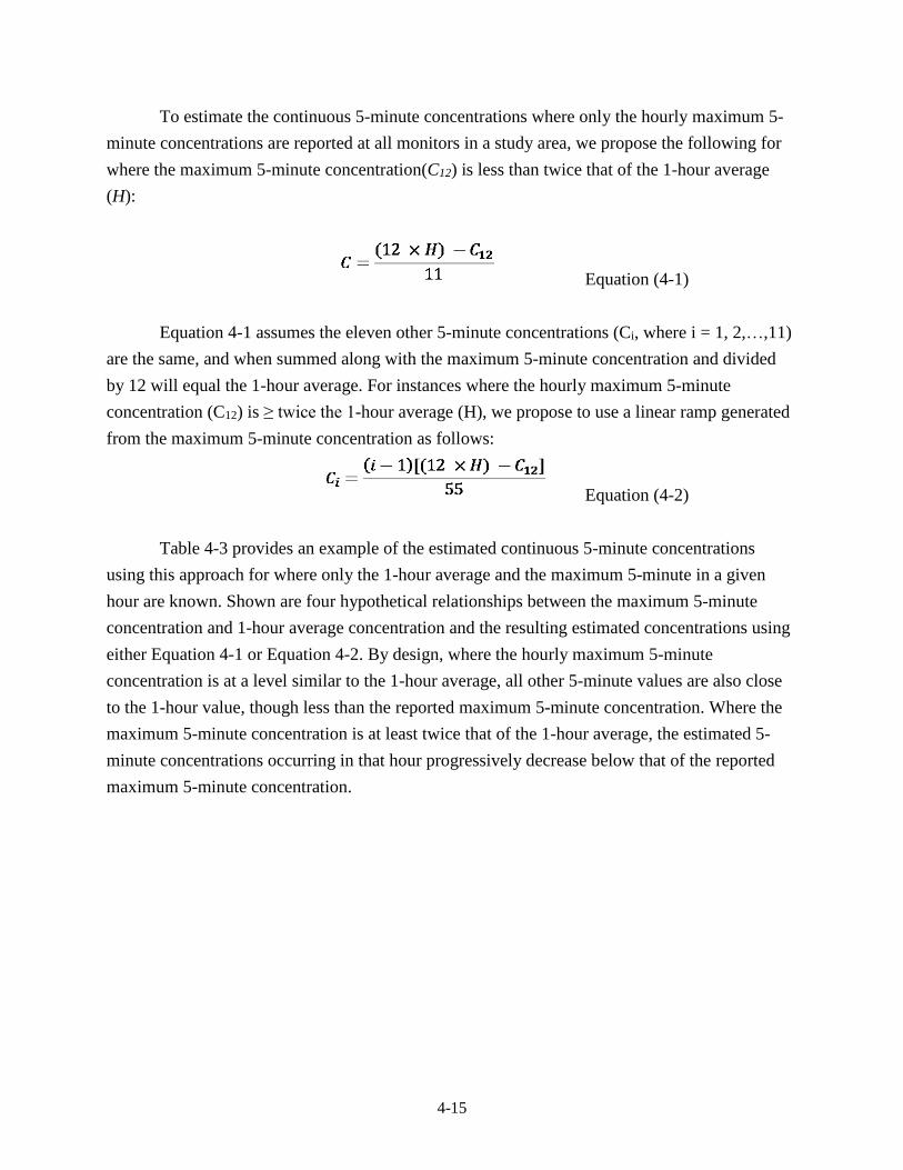
4-15
To estimate the continuous 5-minute concentrations where only the hourly maximum 5-
minute concentrations are reported at all monitors in a study area, we propose the following for
where the maximum 5-minute concentration(C12) is less than twice that of the 1-hour average
(H):
Equation (4-1)
Equation 4-1 assumes the eleven other 5-minute concentrations (Ci, where i = 1, 2,…,11)
are the same, and when summed along with the maximum 5-minute concentration and divided
by 12 will equal the 1-hour average. For instances where the hourly maximum 5-minute
concentration (C12) is ≥ twice the 1-hour average (H), we propose to use a linear ramp generated
from the maximum 5-minute concentration as follows:
Equation (4-2)
Table 4-3 provides an example of the estimated continuous 5-minute concentrations
using this approach for where only the 1-hour average and the maximum 5-minute in a given
hour are known. Shown are four hypothetical relationships between the maximum 5-minute
concentration and 1-hour average concentration and the resulting estimated concentrations using
either Equation 4-1 or Equation 4-2. By design, where the hourly maximum 5-minute
concentration is at a level similar to the 1-hour average, all other 5-minute values are also close
to the 1-hour value, though less than the reported maximum 5-minute concentration. Where the
maximum 5-minute concentration is at least twice that of the 1-hour average, the estimated 5-
minute concentrations occurring in that hour progressively decrease below that of the reported
maximum 5-minute concentration.
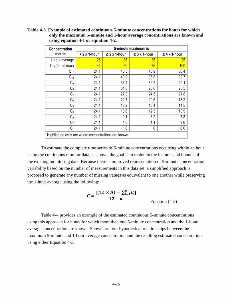
4-16
Table 4-3. Example of estimated continuous 5-minute concentrations for hours for which
only the maximum 5-minute and 1-hour average concentrations are known and
using equation 4-1 or equation 4-2.
Concentration metric
5-minute maximum is
< 2 x 1-hour ≥ 2 x 1-hour ≥ 3 x 1-hour ≥ 4 x 1-hour
1-hour average 25 25 25 25
C12 (5-min max) 35 50 75 100
C11 24.1 45.5 40.9 36.4
C10 24.1 40.9 36.8 32.7
C9 24.1 36.4 32.7 29.1
C8 24.1 31.8 28.6 25.5
C7 24.1 27.3 24.5 21.8
C6 24.1 22.7 20.5 18.2
C5 24.1 18.2 16.4 14.5
C4 24.1 13.6 12.3 10.9
C3 24.1 9.1 8.2 7.3
C2 24.1 4.5 4.1 3.6
C1 24.1 0 0 0.0
Highlighted cells are where concentrations are known.
To estimate the complete time series of 5-minute concentrations occurring within an hour
using the continuous monitor data, as above, the goal is to maintain the features and bounds of
the existing monitoring data. Because there is improved representation of 5-minute concentration
variability based on the number of measurements in this data set, a simplified approach is
proposed to generate any number of missing values as equivalent to one another while preserving
the 1-hour average using the following:
Equation (4-3)
Table 4-4 provides an example of the estimated continuous 5-minute concentrations
using this approach for hours for which more than one 5-minute concentration and the 1-hour
average concentration are known. Shown are four hypothetical relationships between the
maximum 5-minute and 1-hour average concentration and the resulting estimated concentrations
using either Equation 4-3.
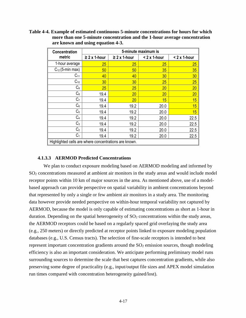
4-17
Table 4-4. Example of estimated continuous 5-minute concentrations for hours for which
more than one 5-minute concentration and the 1-hour average concentration
are known and using equation 4-3.
Concentration metric
5-minute maximum is
≥ 2 x 1-hour ≥ 2 x 1-hour < 2 x 1-hour < 2 x 1-hour
1-hour average 25 25 25 25
C12 (5-min max) 50 50 35 35
C11 40 40 30 30
C10 30 30 25 25
C9 25 25 20 20
C8 19.4 20 20 20
C7 19.4 20 15 15
C6 19.4 19.2 20.0 15
C5 19.4 19.2 20.0 15
C4 19.4 19.2 20.0 22.5
C3 19.4 19.2 20.0 22.5
C2 19.4 19.2 20.0 22.5
C1 19.4 19.2 20.0 22.5
Highlighted cells are where concentrations are known.
4.1.3.3 AERMOD Predicted Concentrations
We plan to conduct exposure modeling based on AERMOD modeling and informed by
SO2 concentrations measured at ambient air monitors in the study areas and would include model
receptor points within 10 km of major sources in the area. As mentioned above, use of a model-
based approach can provide perspective on spatial variability in ambient concentrations beyond
that represented by only a single or few ambient air monitors in a study area. The monitoring
data however provide needed perspective on within-hour temporal variability not captured by
AERMOD, because the model is only capable of estimating concentrations as short as 1-hour in
duration. Depending on the spatial heterogeneity of SO2 concentrations within the study areas,
the AERMOD receptors could be based on a regularly spaced grid overlaying the study area
(e.g., 250 meters) or directly predicted at receptor points linked to exposure modeling population
databases (e.g., U.S. Census tracts). The selection of fine-scale receptors is intended to best
represent important concentration gradients around the SO2 emission sources, though modeling
efficiency is also an important consideration. We anticipate performing preliminary model runs
surrounding sources to determine the scale that best captures concentration gradients, while also
preserving some degree of practicality (e.g., input/output file sizes and APEX model simulation
run times compared with concentration heterogeneity gained/lost).
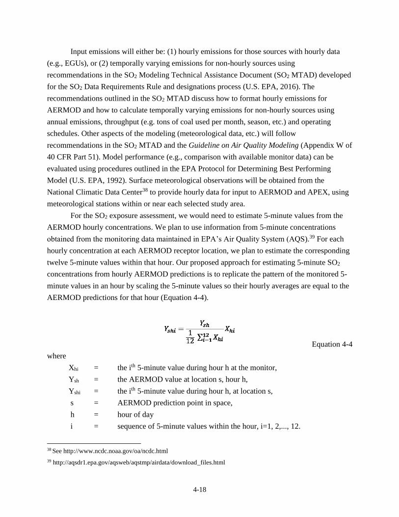
4-18
Input emissions will either be: (1) hourly emissions for those sources with hourly data
(e.g., EGUs), or (2) temporally varying emissions for non-hourly sources using
recommendations in the SO2 Modeling Technical Assistance Document (SO2 MTAD) developed
for the SO2 Data Requirements Rule and designations process (U.S. EPA, 2016). The
recommendations outlined in the SO2 MTAD discuss how to format hourly emissions for
AERMOD and how to calculate temporally varying emissions for non-hourly sources using
annual emissions, throughput (e.g. tons of coal used per month, season, etc.) and operating
schedules. Other aspects of the modeling (meteorological data, etc.) will follow
recommendations in the SO2 MTAD and the Guideline on Air Quality Modeling (Appendix W of
40 CFR Part 51). Model performance (e.g., comparison with available monitor data) can be
evaluated using procedures outlined in the EPA Protocol for Determining Best Performing
Model (U.S. EPA, 1992). Surface meteorological observations will be obtained from the
National Climatic Data Center38 to provide hourly data for input to AERMOD and APEX, using
meteorological stations within or near each selected study area.
For the SO2 exposure assessment, we would need to estimate 5-minute values from the
AERMOD hourly concentrations. We plan to use information from 5-minute concentrations
obtained from the monitoring data maintained in EPA’s Air Quality System (AQS).39 For each
hourly concentration at each AERMOD receptor location, we plan to estimate the corresponding
twelve 5-minute values within that hour. Our proposed approach for estimating 5-minute SO2
concentrations from hourly AERMOD predictions is to replicate the pattern of the monitored 5-
minute values in an hour by scaling the 5-minute values so their hourly averages are equal to the
AERMOD predictions for that hour (Equation 4-4).
Equation 4-4
where
Xhi = the ith 5-minute value during hour h at the monitor,
Ysh = the AERMOD value at location s, hour h,
Yshi = the ith 5-minute value during hour h, at location s,
s = AERMOD prediction point in space,
h = hour of day
i = sequence of 5-minute values within the hour, i=1, 2,..., 12.
38 See http://www.ncdc.noaa.gov/oa/ncdc.html
39 http://aqsdr1.epa.gov/aqsweb/aqstmp/airdata/download_files.html
4-19
Thus, we plan to use the complete calendar year of continuous 5-minute concentrations
and to apply that same concentration variability to the AERMOD receptor, using the complete
time-series of hourly scaling factors (unique to each receptor), to yield the time series of 5-
minute SO2 concentrations (e.g., n= 12*24*365 = 105,120 values) at every receptor in the
exposure modeling domain. Effectively, all spatial gradients that may exist within each hour
across the study area are maintained, the 5-minute monitoring data are adding a finer scale to the
within hour temporal variability. For study areas having only one ambient monitor available to
inform the estimation of 5-minute concentrations, because the within hour temporal variability
will also be maintained (i.e., the 5-minute pattern for the entire year is guided by one monitor),
the spatial gradient across all receptors will also be preserved for every 5-minute concentration.
For instances where a study area has more than one monitor, we propose that the hourly
concentrations predicted at the AERMOD receptors use data from the nearest monitor having 5-
minute concentrations. Again, all spatial gradients that may exist within each hour across the
study area are maintained. However, because there is more than one 5-minute pattern to draw
from and use to generate within hour temporal variability, it is possible that the spatial gradients
observed for the 1-hour do not exactly match the gradients estimated for 5-minute
concentrations. The occurrence of this will likely be limited to a fraction of receptors and during
a limited number of 5-minute periods. The occurrence of this is considered acceptable because
the intent of the overall approach in linking information from both the model and the monitors is
to better inform the air quality surface by using the best of what each approach has to offer.
4.1.3.4 Adjusting Concentrations to Just Meet a Standard
The exposure and risk analyses will be conducted for air quality adjusted to just meet the
existing primary SO2 standard, as well as for recent (unadjusted) air quality. As described in
Chapter 2, a proportional adjustment approach was used in the 2009 REA. An analysis at that
time demonstrated that proportional adjustment is an appropriate approach (Rizzo, 2009). We
have analyzed recent air quality data to evaluate this assumption for purposes of the planned
REA. Focusing on the monitor in each study area having the highest design value during the
2011-2015 period, we compared the monitoring data for a low concentration year with data for a
high concentration year, with low and high defined by having a design value that is either below
(a low year) or above (a high year) the level of the existing standard (99th percentile daily
maximum 1-hour of 75 ppb). Figure 4-6 shows the results for each of the four potential study
areas for monitors having the highest design values, with plots for each of the other monitors
shown in Appendix C.
The results of these new comparisons are similar to what was observed previously
(Rizzo, 2009). In some study areas and at some monitors, there is linearity or proportionality
4-20
when comparing high year to low year concentrations, indicating that adjustments made using a
uniform factor is an acceptable approach to estimating alternative air quality scenarios (e.g.,
Cleveland County, OH; Brown County, WI). Occasionally, there are features of the
concentration distribution that do not entirely reflect a linear/proportional relationship, including
curvilinear features, non-zero regression intercepts, and upper percentile concentrations both
above and below the linear regression line (e.g., Marion County, IN). Given that the adjustment
for the ambient air concentrations considered in the exposure assessment are likely to be small (<
10%, Table 4-1), the impact of deviations from proportionality is also likely to be limited. Thus,
based on these analyses, we plan to use the same proportional adjustment approach in the REA
for the current review as had been used in the 2009 REA, although instances where the potential
impact may be greatest will be evaluated (e.g., in Marion County, IN).
Before adjusting air quality to just meet a standard of interest, typically a design value
(DV) is calculated for locations in the study area. When using a proportional adjustment
approach, the highest DV is used to derive a single multiplicative factor (F) to adjust the
monitored concentrations across the study area. For the planned REA for the current review, in
each study area, F will be calculated by dividing 75 ppb by the DV and will be used to adjust all
SO2 concentrations in a study area by this factor to simulate just meeting the existing standard.
Note, this adjustment of air quality will be based on three years of concentrations, consistent
with the form for the existing standard. For each study area, we will have both a predicted air
quality surface from AERMOD and measurement data from one or more ambient monitors.
Determination of the most appropriate design value to use for adjusting ambient concentrations
in each study area will depend on comparisons of the predicted receptor concentrations with the
monitoring concentrations. Based on this assessment, the adjustment factor(s) selected,
descriptions for how they were derived, and their application will be provided in the REA.
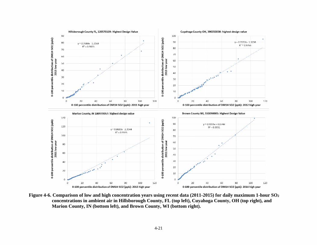
4-21
Figure 4-6. Comparison of low and high concentration years using recent data (2011-2015) for daily maximum 1-hour SO2
concentrations in ambient air in Hillsborough County, FL (top left), Cuyahoga County, OH (top right), and
Marion County, IN (bottom left), and Brown County, WI (bottom right).
4-22
4.1.4 Microenvironmental Concentrations
The SO2 concentrations in each microenvironment (ME) will be estimated using either a
mass-balance or a factors approach, and the user specifies the probability distributions of the
parameters used for the concentration calculations (e.g., indoor-outdoor air exchange rates).
These distributions can flexibly depend on the values of other variables in the model. For
example, the distribution of air exchange rates in a home, office, or car depends on the type of
heating and air conditioning present, which are also stochastic inputs to the model. The user can
choose to retain the value of a stochastic parameter constant for the entire simulation (e.g., house
volume would remain the same throughout the exposure period), or can specify that a new value
shall be sampled hourly, daily, or seasonally from specified distributions. APEX also allows the
user to specify diurnal, weekly, or seasonal patterns for certain ME parameters.
The calculation of ME concentrations in APEX is dependent not only on the parameter
distributions for the mass balance and factors approaches, but also on the ambient (outdoor) air
SO2 concentrations and temperatures. In the 2009 REA, twelve MEs were used to estimate
exposures. In considering the 2009 REA results showing that the majority of peak SO2 exposures
occur outdoors (2009 REA, Figure 8-21) and recognizing the similarity of the focus of the 2009
REA with that of the current REA (i.e., understanding short-term peak exposures), identifying
and distinguishing this number of MEs is unnecessary. We propose to aggregate the number of
MEs, still proposing a core mix that addresses exposures of ambient origin that occur within
indoor, outdoor, and vehicle MEs. For this application to SO2, the following five MEs will be
modeled:
Indoors - residence
Indoors - all other (e.g., offices, shopping)
Outdoors - all other (e.g., residence, public parks)
Outdoors - near-road (e.g., near-road, public garage)
In vehicles (e.g. automobile, bus)
Parameters defining each microenvironment will be specified by distributions that reflect
the variability of these parameters. The parameters used depend on whether a microenvironment
is modeled using the factor-based model or the mass balance model. We will not be modeling
indoor sources of SO2 in this analysis, because our focus is on exposure to SO2 of ambient air
origin.40 We still expect the outdoor MEs to be the most important regarding peak 5-minute SO2
40 Indoor SO2 sources can include secondary heating sources (e.g., fireplaces, space heaters), however, personal SO2
exposure measurements have generally been lower than ambient air concentrations, indicating personal exposure
to generally be dominated by ambient air exposure (2008 ISA, section 2.6.3; second draft ISA, section 3.4.1).
4-23
exposures, based on a finding in the 2009 SO2 REA indicating peak exposures occurred much
more frequently in outdoor MEs than within indoor and vehicle MEs (second draft ISA, p. 3-23).
We plan to use a factor-based model to simulate the outdoors and outdoors near-road
MEs, for which the mass-balance model is not applicable, and also the in-vehicles ME, for which
adequate data are not available to use the mass-balance model. Two parameters affect the
pollutant concentration calculation in the factors method, the proximity and infiltration factors.
The proximity factor (FPR) is a unitless parameter that represents the relationship of the ambient
air concentration outside of the ME (CO) to the concentration at a monitoring station (CA) by the
equation CO = FPR CA. The infiltration factor (Finf) is a unitless parameter that represents the
equilibrium fraction of pollutant entering a ME from outside the ME. The concentration inside
the ME (CI) is estimated by the equation CI = Finf CO. The infiltration factor in the factor-based
model is often expressed as:
ka
PaF
inf
where P is a penetration coefficient, a is an air exchange rate, and k is a loss rate. APEX draws
values of these parameters from ME-specific distributions specified by the user, to model the
stochastic nature of these factors. In a practical sense, the infiltration factor for modeling outdoor
MEs are assumed equal to 1.
The mass balance model is more appropriate for complex MEs and where data are
available to model such MEs. We plan to use the mass balance model for the indoor MEs. The
mass balance model assumes that an enclosed ME (e.g., a room in a residence) is a single well-
mixed volume in which the air concentration is approximately spatially uniform. APEX
estimates the concentration of an air pollutant in such a ME by using the following three
processes:
Inflow of air into the ME
Outflow of air from the ME
Removal of a pollutant from the ME due to deposition, filtration, and chemical
degradation
In addition to proximity factors, the mass balance model supports parameter distributions
for time varying emissions sources, decay rate, air exchange rate, volume, and removal rate. We
plan to estimate the distributions of these ME-specific parameters based on existing data used for
2009 REA and other recent REAs (e.g., the 2014 O3 REA) and update these parameters using
any newly available information, where appropriate. The description of the final ME-specific
parameters, their sources of information, and an assessment of representativeness will be
provided in the REA.
4-24
4.1.5 At-Risk Populations
The second draft ISA identifies people with asthma to be at increased risk of respiratory-
related effects associated with short-term peak SO2 exposures (second draft ISA, Table 6-7 and
section 6.3.1).41 As discussed in section 4.2 below, controlled human exposure studies support
this conclusion and provide information on exposure duration and concentrations associated with
effects in people with asthma. In addition to characterizing exposure and risk for adults with
asthma, we will also develop separate exposure and risk estimates for school-aged children (ages
5-18) with asthma, as the evidence indicates that children with asthma may be at increased risk
compared to adults with asthma. Children under the age of 5 will not be included in this
assessment because the CHAD database has relatively fewer activity patterns in the database to
represent that population group42 compared with those for school-age children and that there may
be greater uncertainty in estimating important physiological attributes (e.g., their activity specific
METs). Use of this age group is consistent with REAs performed for other NAAQS pollutants
(e.g., 2014 O3 REA, 2010 NO2 REA).
4.1.6 Simulated Individuals
As summarized in section 2.3.2.2, APEX stochastically generates a user-specified
number of simulated persons to represent the population in the study area. The number of
simulated individuals can vary and depends on the size of the population to be represented,
though we expect the number of simulated individuals to be about 50,000 – 100,000. Each
simulated person is represented by a “personal profile.” The personal profile includes
characteristics such as a specific age, a specific home sector, a specific work sector (or does not
work), specific housing characteristics, specific physiological parameters, and so on. The profile
does not correspond to any particular individual in the study area, but rather represents a
simulated person. While a single profile does not have much meaning in isolation, a collection of
profiles represents a random sample drawn from the study area population. This means that
statistical properties of the collection of profiles should reflect statistical properties of the actual
population in the study area.
As summarized in section 2.3.2, APEX generates population-based exposures through the
use of several population databases. Based on the defined study area and study groups, APEX
will simulate representative individuals using appropriate geographic, demographic, and health
41 There are several other population groups evaluated in the second draft ISA, however only people with asthma
were considered as having adequate evidence for potential increased SO2 exposure and increased risk of SO2-
related health effects (second draft ISA, section 6.6).
42 Based on the most recent CHAD database, the limited amount of activity pattern information mainly affects
diaries for children aged 0 to < 2 years old.
4-25
status information provided by existing population-based surveys. APEX generates the simulated
person or profile by probabilistically selecting values for a set of profile variables such as
demographic variables, which are defined by the 2010 U.S. Census data, personal and
physiologic attributes (described below), and other modeling variables.
Once the immediate demographic variables are identified by APEX for a simulated
individual in the study area, the other variable values are selected as well as the development of
the activity patterns that account for the places the simulated individual visits and the activities
they perform. The following subsections describe the population data we plan to use in the
assessment to assign key features of the simulated individuals, and approaches used to simulate
the basic physiological functions important to the exposure estimates for this REA.
4.1.6.1 Population Demographic Information
To stochastically simulate the population of interest, APEX will use probability
distributions derived from the 2010 Census. In the past, we have most commonly done this at a
census tract level, though it is possible to do so at the block-level. Determination of the most
appropriate spatial scale to use will be based on evaluations of the spatial heterogeneity in SO2
concentrations in the selected study areas (section 4.1.3.3) and a practical consideration of the
anticipated impact to exposures of finer-scale modeling weighed against the resources needed to
perform the modeling at that scale. Regardless, we plan to use population counts from the 2010
Census of Population and Housing Summary File 1.43 Summary File 1 (SF 1) contains what the
Census program calls “the 100-percent data,” which is the information compiled from the
questions asked of all (100% of) people and housing units in the U.S.
In the 2010 U.S. Census, estimates of employment were developed by census tract and
will be used in the REA. The file input to APEX will be broken down by sex and age group, so
that each sex/age group combination is given an employment probability fraction (ranging from
zero to one) within each census tract. The age groupings in this file currently are: 16-19, 20-21,
22-24, 25-29, 30-34, 35-44, 45-54, 55-59, 60-61, 62-64, 65-69, 70-74, and greater than 75 years
of age. Because there is no employment information for children under 16 years of age,
simulated individuals in that age group are assumed to be unemployed and will be given an
employment probability fraction of zero.
4.1.6.2 Asthma Prevalence
In previous REAs for which people with asthma are a simulated at-risk population, we
have attempted to account for common factors that are known to influence observed asthma
43 Technical documentation - 2010 Census Summary File 1—Technical Documentation/prepared by the U.S.
Census Bureau, Revised 2012 - available at: http://www.census.gov/prod/cen2010/doc/sf1.pdf.
4-26
prevalence, such as age, sex, and U.S region. In better accounting for these factors, we could
better represent the estimated exposures that these potentially at-risk population groups might
experience. For the 2014 O3 REA in particular, we expanded the list of potential influential
factors to not only address person-level attributes but to also include a more specific geographic-
level attribute to better link the potentially at-risk population group(s) to spatially heterogeneous
ambient concentrations. This was motivated by observations that (1) there are notable differences
in asthma prevalence by age, gender, region, and poverty status, (2) there is variability in the
spatial distribution of poverty status across census tracts, stratified by age, and (3) there is spatial
variability in local scale ambient concentrations of many air pollutants, we developed a database
that provides estimates of asthma prevalence at a census tract level (2014 O3 REA, Appendix C).
We have updated the previously used database to include recent demographic
information obtained from the U.S. Census for use in this current REA.44 The same asthma
prevalence (2006-2010) was included, originally obtained from the Center for Disease Control
(CDC) and Prevention’s National Health Interview Survey (NHIS).45 The asthma prevalence was
stratified by NHIS defined regions (Midwest, Northeast, South, and West), sex, age (single years
for ages 0-17) or age groups (ages ≥ 18), and by a family income/poverty ratio.46 Asthma
prevalence was then linked to U.S. census tract level poverty ratio probabilities, also stratified by
age and age groups, to generate a final database consisting of census tract level asthma
prevalence for the entire U.S. A summary of the asthma prevalence approximated for each
potential study area is provided in Table 4-5. The updated database containing asthma prevalence
stratified by age (or age groups) and sex for each tract in the selected study areas will be
provided as part of the REA.
44 Summary tables (B17024) used from the 5-year American Community Survey data for 2008-2012 are available
at: https://factfinder.census.gov/faces/tableservices/jsf/pages/productview.xhtml?src=bkmk
45 See http://www.cdc.gov/nchs/nhis.htm (accessed October 4, 2011).
46 The income/poverty ratio threshold used was 1.5, that is the surveyed person’s family income was considered
either ≤ or > than a factor of 1.5 of the US Census estimate of poverty level for the given year.
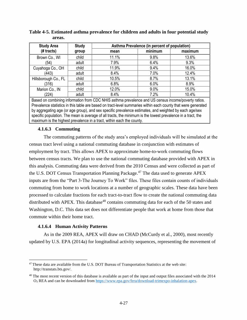
4-27
Table 4-5. Estimated asthma prevalence for children and adults in four potential study
areas.
Study Area (# tracts)
Study group
Asthma Prevalence (in percent of population)
mean minimum maximum
Brown Co., WI (54)
child 11.1% 9.8% 13.6%
adult 7.9% 6.4% 9.3%
Cuyahoga Co., OH (443)
child 11.9% 9.4% 16.0%
adult 8.4% 7.0% 12.4%
Hillsborough Co., FL (316)
child 10.5% 8.7% 13.1%
adult 6.8% 6.0% 8.9%
Marion Co., IN (224)
child 12.0% 9.0% 15.0%
adult 8.4% 7.2% 10.4%
Based on combining information from CDC NHIS asthma prevalence and US census income/poverty ratios. Prevalence statistics in this table are based on tract-level summaries within each county that were generated by aggregating age (or age group), and sex specific prevalence estimates, and weighted by each age/sex specific population. The mean is average of all tracts, the minimum is the lowest prevalence in a tract, the maximum is the highest prevalence in a tract, within each the county.
4.1.6.3 Commuting
The commuting patterns of the study area’s employed individuals will be simulated at the
census tract level using a national commuting database in conjunction with estimates of
employment by tract. This allows APEX to approximate home-to-work commuting flows
between census tracts. We plan to use the national commuting database provided with APEX in
this analysis. Commuting data were derived from the 2010 Census and were collected as part of
the U.S. DOT Census Transportation Planning Package.47 The data used to generate APEX
inputs are from the “Part 3-The Journey To Work” files. These files contain counts of individuals
commuting from home to work locations at a number of geographic scales. These data have been
processed to calculate fractions for each tract-to-tract flow to create the national commuting data
distributed with APEX. This database48 contains commuting data for each of the 50 states and
Washington, D.C. This data set does not differentiate people that work at home from those that
commute within their home tract.
4.1.6.4 Human Activity Patterns
As in the 2009 REA, APEX will draw on CHAD (McCurdy et al., 2000), most recently
updated by U.S. EPA (2014a) for longitudinal activity sequences, representing the movement of
47 These data are available from the U.S. DOT Bureau of Transportation Statistics at the web site:
http://transtats.bts.gov/.
48 The most recent version of this database is available as part of the input and output files associated with the 2014
O3 REA and can be downloaded from https://www.epa.gov/fera/download-trimexpo-inhalation-apex.
4-28
simulated individuals through time and space.49 The locations used in the CHAD diaries are
assigned to the specified APEX MEs.50 For each event51 in an individual’s activity pattern,
APEX calculates the concentration in the associated ME (see section 4.1.4 above). The model
then combines the event-specific exposures to obtain a continuous time-series of exposures
spanning the time period of interest. For SO2, as summarized in section 2.3.2 above, it is
important to have an understanding of exertion levels associated with each activity. CHAD
contains statistical distributions of activity-specific METs developed from literature-derived
data, which are used to estimate the energy expended (and associated breathing rates) while an
individual performs particular activities. Further details regarding the METs distributions and
related physiological algorithms used in the current version of APEX are provided in U.S. EPA
(2012b).
Further, when performing multiday simulations, an approach is needed to generate the
longitudinal series of diary days for each simulated individual because most of the diary data in
CHAD are cross-sectional, i.e., the information that originated from the surveyed individual
captured only a single or few consecutive days of their activity patterns. To overcome this
limitation, APEX provides three methods of assembling composite diaries. The first (basic)
method, which is adequate for estimating mean exposures, simply involves randomly selecting
an appropriate activity diary for the simulated individual from the available diary pool. The
second method is a more complex algorithm for assembling longitudinal diaries that realistically
simulates day-to-day (within-person correlations) and between-person variation in activity
patterns (and thus exposures). The third method uses a Markov-chain clustering algorithm to also
recreate realistic patterns of day-to-day variability.
For this application we plan to use the second approach to capture the tendency of
individuals to repeat activities, based on reproducing realistic variation in a key diary variable
(Glen et al., 2008). For this SO2 exposure and risk assessment, the key variable selected is the
amount of time an individual spends outdoors each day, one of the most important determinants
of exposure to high levels of SO2 (second draft ISA, section 3.4.1). This longitudinal method
49 The sequences generated by CHAD account for factors such as particular day-types (e.g., weekday versus
weekend) and outdoor temperature, and how they influence daily activities and peoples’ exposures. The data
contained within CHAD come from multiple surveys with varied structures, though in general, the surveys have a
central commonality based on their containing daily diaries of human activity information. Relevant demographic
attributes of these individuals, such as age and sex, are included as well.
50 There are many more CHAD locations than MEs being modeled (there are over 100 CHAD locations and five
MEs to be modeled in this assessment). Thus, most of the MEs will have multiple CHAD locations mapped to
them.
51 Exposure events are when an individual is in a single microenvironment, exposed to a constant concentration for a
specific duration of time, and while at a constant activity level. The duration of the event is a maximum of 1 hour
due to the structure of the time-location-activity diary, but could be as short as 1 minute.
4-29
targets two statistics, a population diversity statistic (D) and a within-person autocorrelation
statistic (A). Values of 0.2 for D and 0.2 for A were initially developed based on analyses by
Geyh et al. (2000) and Xue et al. (2004), with both studies evaluating groups of children ages 7
to 12 in a single study area. We may adjust values for D upwards to 0.5 to reflect a broader range
of ages and to better estimate repeated activities. Further details regarding the development of
the longitudinal methodology can be found in U.S. EPA (2012b).
4.1.6.5 Personal Attributes
In addition to the above demographic information in constructing simulated individuals,
each modeled person can be assigned status and personal attributes. All of these variables are
treated probabilistically in APEX, taking into account interdependencies where possible, and
reflecting variability in the population. The EPA regularly makes improvements to APEX. If
additional updates regarding new approaches or data are completed in time for use in the REA
for this review, then these updates will be fully described in the new REA.
4.1.6.5.1 Status Attributes
Status variables are factors deemed important in estimating ME concentrations, and can
include, but are not limited to, people’s housing type, whether their home has air conditioning,
and whether their car has air conditioning. Because outdoor MEs are expected to contribute the
most to an individuals’ highest exposure (and potential health risk) and these factors largely
pertain to indoor MEs, further details regarding these will be provided in the REA.
4.1.6.5.2 Physical Attributes
Personal attributes can be important when estimating pollutant specific dose and can
include height, weight, and body surface area. Two key personal attributes determined for each
individual in this assessment are body mass and BSA. Each simulated individual’s body mass is
randomly sampled from recently updated age- and sex-specific body mass distributions and
generated from NHANES data for the years 2009-2014.52 Then age- and sex-specific body
surface area can be estimated for each simulated individual.
4.1.6.5.3 Ventilation Rate
Human activities are variable over time, and a wide range of activities are possible even
within a single hour of the day. The type of activity an individual performs, such as sleeping or
jogging, will influence their ventilation rate. APEX estimates minute-by-minute ventilation rates
that account for the expected variability in the activities performed by simulated individuals. The
second draft ISA indicates that the lung function responses associated with short-term peak SO2
52 Original data are available at https://wwwn.cdc.gov/nchs/nhanes/Default.aspx. Actual distributions used will be
part of the APEX input/output file package generated for this REA.
4-30
exposures coincide with moderate or greater exertion (second draft ISA, section 5.2.1.2). In our
exposure modeling approach, we will use APEX to generate the complete time series of activity-
specific ventilation rates and the corresponding time-series of estimated SO2 exposures. APEX
will then aggregate both the ventilation rate and exposure concentration to the averaging time of
interest (a 5-minute average). Thus, the model will provide exposure estimates for the simulated
individuals that pertain to specific target levels for both ventilation rate and exposure
concentration. The approach to estimating activity-specific energy expenditure and associated
ventilation rate involves several algorithms and physiological variables (U.S. EPA, 2012a,b). As
described in section 3.4.3, we are nearing completion of an updated approach to estimate
activity-specific V̇E.
4.1.7 Exposure Assessment Estimates
There are several useful indicators of individuals’ exposures to various levels of air
pollution. Factors that can be important in defining such indicators include the magnitude and
duration of exposures, frequency of repeated high exposures, and ventilation rate of the
individual at the time of exposure. In this assessment, exposure indicators will include the
occurrence of daily maximum 5-minute SO2 exposures at or above benchmark levels, also
stratified by a specified target ventilation rate(s). Given the nature of these indicators with regard
to informing potential health risk, details as to the selection of these particular target levels are
provided in section 4.2.2.
APEX can calculate two general types of summary exposure estimates: counts of people
and person-occurrences. The former counts the number of individuals exposed one or more times
per year, several times a year (e.g., 5 or more times) to the exposure indicator (e.g., exposure
level and ventilation rate) of interest. In the case where the exposure indicator is a benchmark,
the model estimates the number of people who experience that level of air pollution, or higher, at
least once during the modeled period. The person-occurrences metric counts the number of times
that an individual is exposed to the exposure indicator of interest and then accumulates counts
over all individuals. For example, a value of 10 for the person-occurrences measure could be the
result of 1 occurrence for 10 people or 10 occurrences for 1 person. Because this latter metric is
less informative regarding individual exposures, we do not anticipate reporting this output for
this REA.
In summary, APEX modeling outputs for use in this review will include (1) counts of
people exposed at least once to a range of short-term peak SO2 concentrations while at or above
a particular exertion level, and (2) counts of people experiencing multiple exposures at or above
a particular level while at or above a given exertion level.
4-31
4.2 HEALTH RISK CHARACTERIZATION
In this section, we describe the two approaches we will use to characterize potential risk.
As in the last review, these approaches are based on the body of evidence from the controlled
human exposure studies reporting lung function decrements (as measured by changes in sRaw
and FEV1), as well as changes in other measures of lung function, respiratory symptoms, and
various markers of inflammation, in adult study subjects having asthma. For both approaches,
staff plans to develop health risk estimates for two groups of individuals with asthma living in
the selected study areas: adults with asthma (ages > 18), and school-aged children with asthma
(ages 5-18).
4.2.1 Health Endpoints
As in the last review, the evidence of health effects associated with exposure to short-
term (5-10 minutes) peak SO2 exposures is based on findings from controlled human exposure
studies of exercising adult individuals with asthma, most of which were conducted in the 1980s
and evaluated in the ISA from previous and current NAAQS reviews (2008 ISA; second draft
ISA). Specifically, the health endpoints identified in those studies include changes in respiratory
function indicative of bronchoconstriction as measured by increased specific airway resistance
(sRaw) and decreased forced expiratory volume in one second (FEV1) observed in subjects with
asthma. As summarized in section 2.1.3 above, exercising individuals with asthma exposed to
SO2 concentrations of 200-300 ppb for 5-10 minutes experienced moderate or greater lung
function decrements (increases in sRaw ≥ 100%) in 5-30% of tested individuals. Exercising
individuals with asthma exposed to SO2 concentrations of 400-600 ppb for to 5-10 minutes
resulted in moderate or greater decrements in lung function in 20-60% of tested individuals. At
concentrations ≥ 400 ppb, moderate or greater decrements were frequently accompanied by
respiratory symptoms.
This evidence of responses associated with bronchoconstriction in exercising individuals
with asthma is the focus of the two approaches to be used to characterize health risk:
(1) comparison of exposures at elevated ventilation to exposure concentrations of potential
concern (benchmark levels), and (2) lung function risk estimates.
4.2.2 Target Ventilation Rates
As in the last review, we recognize that the target ventilation rate for study subjects (i.e.,
male and female adults) experiencing effects from 5-10 minute SO2 exposures in most of the
4-32
controlled human exposure studies was approximately between 40-50 L/min (Table 4-6).53 In
order to use this information to estimate health risks for children, the ventilation targets for adults
need to be adjusted to best reflect the different physiology of children. One approach to
accomplish this is to generate an equivalent ventilation rate (EVR) based on normalizing the
simulated individuals’ activity-specific ventilation rate to their BSA. Staff has used an EVR in
REAs for previous SO2 and O3 NAAQS REAs to also identify comparable activity-specific
ventilation rates for children and adults (U.S. EPA, 2014b; Whitfield et al., 1996).
As was done in previous REAs, we propose the same approach to be used here. The
target ventilation rates from the controlled human exposure study are generally within 40-50
L/min, with most at or around 40 L/min. However, body surface area was not measured in the
controlled human exposure studies and the relevant ventilation data were not separated by sex.
Staff assumed a median estimate of BSA of 1.95 m2 based on data for males and females
within the ages of 21-50 from U.S. EPA (2011) were reasonable estimates of the study subjects.
Based on these data, an EVR = 40/1.95 ≈ 21 L/min-m2 will be used to characterize an equivalent
target ventilation rate in this assessment. Thus, individuals at or above an EVR of 21 L/min-m2
(children or adult) for a 5-minute exposure event are characterized as performing activities at or
above moderate exertion. This EVR is slightly lower than that used in the 2009 SO2 REA (i.e.,
22 /min-m2) because the BSA (1.8 m2) approximated at that time was based on data from U.S.
EPA (1997), thus possibly comprised of a relatively fitter population.
4.2.3 Exposure Benchmark-Based Health Risk
As in the last review (as described in section 2.4.3 above), one of the risk metrics to be
estimated will be based on comparisons of estimates of 5-minute exposures experienced while at
an elevated ventilation rate to benchmark levels based on the controlled human exposure studies.
In addition to its use in the 2009 SO2 REA, this approach has been used in past O3 REAs (e.g.,
U.S. EPA, 2014b). In the subsections that follow, each of these elements are evaluated and
defined to objectively inform the characterization of the potential health risk associated with the
APEX simulated individuals’ exposure events.
4.2.3.1 Benchmark Levels
As in the 2009 REA, we have identified a set of benchmarks to represent “exposures of
potential concern” (75 FR 35527, June 22, 2010), 5-minute concentrations for which there is
potential for a respiratory response indicative of some level of bronchoconstriction to occur in an
53 Note that study subjects were free-breathing; thus it is expected that there was a mixture of nasal, oral, and oro-
nasal breathing that occurred across the study subjects. Without information regarding the precise breathing
method used by any subject corresponding with their health response, staff assumed that the mixture in breathing
method used by study subjects is representative for the simulated population.
4-33
exposed individual, with the potential and the severity varying with the magnitude of the
benchmark level. These levels are derived solely from the controlled human exposure studies,
which can examine the health effects of SO2 in the absence of co-pollutants that typically can
confound results in epidemiologic analyses; thus, health effects observed in such controlled
studies can confidently be attributed to a defined exposure level of SO2.
Considering this information, as described in the second draft ISA and summarized in
section 2.2.3 above, staff concludes that it is appropriate, as in the last review, to use four
benchmark levels: 100, 200, 300 and 400 ppb. As recognized in the last review, we consider
exposures with respect to the 200 and 400 ppb 5-minute benchmark levels to be of particular
interest because: (1) 400 ppb represents the lowest concentration in free-breathing controlled
human exposure studies where moderate or greater lung function decrements occurred which
were often statistically significant at the group mean level and were frequently accompanied by
respiratory symptoms; and (2) 200 ppb is the lowest level at which moderate or greater lung
function decrements in free-breathing controlled human exposure studies were found in some
individuals, although these lung function changes were not statistically significant when
evaluated considering the group mean level (75 FR 35527, June 22, 2010). The lowest level (100
ppb) has been identified in consideration of the data showing moderate or greater lung function
decrements at the lowest exposure concentration tested in free breathing exposure studies (200
ppb) and of the very limited data indicating some potential for SO2-induced lung function
decrements in individuals with asthma54 exposed to 100 ppb SO2 administered via mouthpiece55
(second draft ISA, section 5.2.1).
4.2.3.2 Exposure Benchmark-based Risk Results
APEX estimates of personal exposure will be compared to the health benchmark levels,
considering also that the exposures occurred while at or above the target ventilation rate, an
approach best resembling the conditions of the controlled human exposure study. As described in
54 We have also considered the evidence with regard to the response of individuals with severe asthma that are not
generally represented in the full set of controlled human exposure studies. There is no evidence to indicate such
individuals would experience moderate or greater lung function decrements at lower SO2 exposure concentrations
than individuals with moderate asthma. With regard to the severity of the response, the limited data that are
available indicate a similar magnitude SO2-specific response (in sRAW) as that for individuals with less severe
asthma, although the individuals with more severe asthma are indicated to have a greater response to exercise
prior to SO2 exposure, indicating that those individuals “may have more limited reserve to deal with an insult
compared with individuals with mild asthma” (second draft ISA, p. 5-21).
55 Studies utilizing a mouthpiece to deliver pollutant concentrations cannot be directly compared to studies involving
freely breathing subjects, as nasal absorption of SO2 is bypassed during oral breathing, thus allowing a greater
fraction of inhaled SO2 to reach the tracheobronchial airways. As a result, individuals exposed to SO2 through a
mouthpiece are likely to experience greater respiratory effects from a comparable SO2 exposure using free
breathing.
4-34
section 4.2.1, when the exposure outcome is linked with the appropriate exertion level, a more
appropriate indicator of potential health risk is generated than when compared with an approach
that considers ambient air concentrations or exposures alone. Thus, the time-series of exposures
for each APEX-simulated individual will be used to identify the daily maximum 5-minute SO2
concentrations that occur while at moderate or greater exertion. We will focus on the daily
maximum 5-minute exposure relative to the benchmark levels to capture the maximum potential
response an individual would experience in a given day, rather than comparing all 5-minute
exposures to each benchmark. While there is limited evidence that the SO2-specific
bronchoconstriction response is transient, such that similar responses might be expected from
two appropriately-separated exposures in the same day (e.g., Linn et al., 1984; Linn et al., 1987),
the interpretation of the multiple occurrences within a day could be complicated by the need to
consider other factors, such as duration of both the exposure and associated elevated activity
level, as well as disease status (second draft ISA, section 5.2.1). Based on all of the instances
when a daily maximum 5-minute exposure (while at or above the target EVR) is above a
benchmark level, APEX will then summarize the individual-level information and generate a
population-based, study area statistic indicating the number (and percent) of simulated persons
experiencing exposures at or above the particular benchmark levels of interest, while at moderate
or greater exertion.56
4.2.4 Lung Function Decrement-based Health Risk
The lung function risk assessment will involve an estimation of the number of people
expected to experience a specific lung function effect and the total number of occurrences of
these effects per individual across the simulation period. Thus two risk metrics are generated.
The first would indicate the number and percent of people estimated to at least one lung function
decrement in a year. The second risk metric would indicate the number and percent of people
experiencing multiple lung function decrements associated with SO2 concentrations. This
assessment requires the combining of E-R functions discussed below (section 4.2.4.1) with the
exposures estimates for the relevant exposure duration (5 minutes) and exertion level.
4.2.4.1 Development of Exposure-Response Functions
The health risk assessment conducted in this new review will build on the approach
developed and applied in the 2009 REA. In that assessment, risk estimates were developed for
56 A ‘person-days’ risk metric can also be generated by APEX, indicating the total number of exceedances across the
modeling domain and time period assessed as a whole, but this metric is less informative for the purposes of the
review. The metric conflates the variability in individual exposures (this can be wide ranging depending on the
occurrence of peak concentrations and the distribution of time spent outdoors for modeled individuals), and from
a physiological perspective, creates an uninterpretable aggregate population exposure metric.
4-35
lung function responses associated with 5-minute exposures while engaged in moderate or higher
exertion. These estimates were based on E-R relationships estimated from the combined data sets
from multiple controlled human exposure studies. The data from these studies were corrected for
effects observed with exposure to clean air to remove any systematic bias that might be present
in the data attributable to exercise, diurnal variation, or other effects, in addition to those
attributed by exposure to SO2, during the course of an exposure.
The E-R functions will be derived by applying a regression approach to these data for the
selected health endpoints. Probit and logistic regression techniques have been used previously to
mathematically describe the E-R relationship (2009 SO2 REA, section 9.2.3). We plan to use the
probit model for this risk analysis based on comments from CASAC on the use of this approach
in the 2009 REA (Samet, 2009, p. 14).57 Because there are fewer clinical data for FEV1 than for
sRaw (second draft ISA, Table 5-2) and there is greater physiological specificity in the sRaw
measurement compared to that of the FEV1, we will estimate health risk only using the sRaw
data in this assessment. This reasoning and conclusion is consistent with that of the last review.
Whereas FEV1 risk estimates were calculated and presented in the 2009 REA, they were given
less weight than risk estimates based on sRaw in considerations for the review (2009 REA,
chapter 10; 75 FR 35520).
To evaluate health risk in this assessment, we will estimate numbers and percent of study
groups expected to experience moderate or greater lung function decrements, in terms of
increases in sRaw at or above 100% and at or above 200%, as a result of exposures to SO2 from
ambient air. There are two controlled human exposure studies of the effects of SO2 on lung
function that were not used in the 2009 REA analyses (Linn et al., 1983; Horstman et al.,
1986).58 These studies, in addition to the studies used in the 2009 REA, will be included in the
dataset used to derive the E-R functions. Table 4-6 presents study summary data for changes in
sRaw from all references from which individual data are available, for free-breathing studies. To
illustrate the E-R relationship indicated by these data, the percent of the study populations
experiencing changes in sRaw (∆sRaw) ≥ 100% is plotted in Figure 4-7, where the points are
annotated with the number of subjects from each study.
The data used, of course, are important in determining the E-R function. Of particular
interest is how the function extends below exposures for which we have controlled human
57 From Samet, 2009 (p. 14): “Another issue for clarification is the choice to base predictions of sRaw responses
only on a fit to the logistic model. A probit model fit is considered but the discussion is based only on goodness-
of-fit criteria which are reportedly equivalent between the two models. This neglects the a priori reason to prefer
the probit model (based on a hypothesized lognormal distribution of individual thresholds for response).”
58 The individual-level data from Linn et al (1983) were not available at the time of the 2008 ISA. The Horstman et
al. 1986 data were interpreted based on the figures provided in that paper indicating individual responses.
4-36
exposure data (i.e., < 200 ppb). In the 2009 REA, apportioning of the risk by the selected
exposure levels indicated that low level 5-minute exposures (e.g., 0-50 ppb, 50-100 ppb, 100-150
ppb, etc.) can contribute to a large portion (50% or more) of the estimated risk depending on the
air quality scenario (e.g., 2009 REA, Figure 9-8). For instance, the range of SO2 exposures and
associated responses included from the higher end can have varying influence on the E-R
function at the lower end. To demonstrate this, we derived the function using two data sets: one
E-R function derived using all of the data in Table 4-6 and one derived without using the 1000
ppb exposure results. For each respective function, the associated model predictions were
generated at 5 ppb exposure increments, indicating the response probabilities at each exposure
level. Table 4-7 provides the results of this comparison for exposures at or below 100 ppb. Based
on these preliminary analyses, it can be seen that the choice of data used to derive the E-R
function can influence the percent of the population estimated to have a response by a factor of 2
or more. How this can influence the number of simulated individuals is not known at this time,
however, we expect to perform additional analyses of the E-R function such as this, along with
others, to provide additional perspective in the current REA.
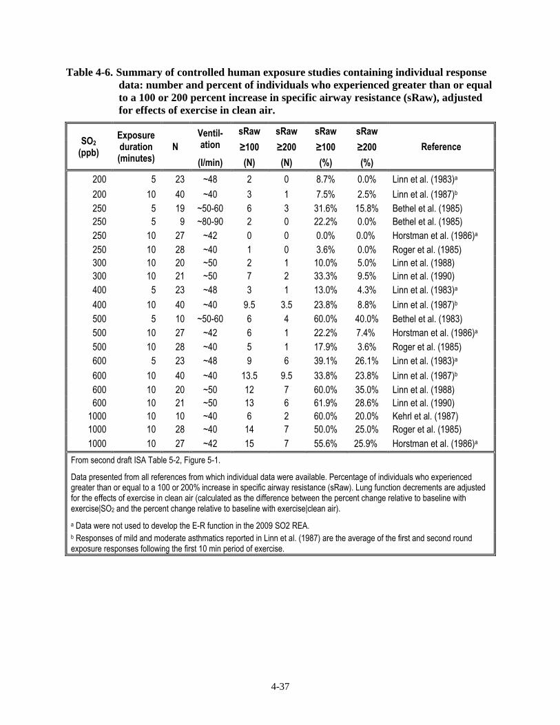
4-37
Table 4-6. Summary of controlled human exposure studies containing individual response
data: number and percent of individuals who experienced greater than or equal
to a 100 or 200 percent increase in specific airway resistance (sRaw), adjusted
for effects of exercise in clean air.
SO2 (ppb)
Exposure duration (minutes)
N
Ventil- ation
sRaw sRaw sRaw sRaw
Reference ≥100 ≥200 ≥100 ≥200
(l/min) (N) (N) (%) (%)
200 5 23 ~48 2 0 8.7% 0.0% Linn et al. (1983)a
200 10 40 ~40 3 1 7.5% 2.5% Linn et al. (1987)b
250 5 19 ~50-60 6 3 31.6% 15.8% Bethel et al. (1985)
250 5 9 ~80-90 2 0 22.2% 0.0% Bethel et al. (1985)
250 10 27 ~42 0 0 0.0% 0.0% Horstman et al. (1986)a
250 10 28 ~40 1 0 3.6% 0.0% Roger et al. (1985)
300 10 20 ~50 2 1 10.0% 5.0% Linn et al. (1988)
300 10 21 ~50 7 2 33.3% 9.5% Linn et al. (1990)
400 5 23 ~48 3 1 13.0% 4.3% Linn et al. (1983)a
400 10 40 ~40 9.5 3.5 23.8% 8.8% Linn et al. (1987)b
500 5 10 ~50-60 6 4 60.0% 40.0% Bethel et al. (1983)
500 10 27 ~42 6 1 22.2% 7.4% Horstman et al. (1986)a
500 10 28 ~40 5 1 17.9% 3.6% Roger et al. (1985)
600 5 23 ~48 9 6 39.1% 26.1% Linn et al. (1983)a
600 10 40 ~40 13.5 9.5 33.8% 23.8% Linn et al. (1987)b
600 10 20 ~50 12 7 60.0% 35.0% Linn et al. (1988)
600 10 21 ~50 13 6 61.9% 28.6% Linn et al. (1990)
1000 10 10 ~40 6 2 60.0% 20.0% Kehrl et al. (1987)
1000 10 28 ~40 14 7 50.0% 25.0% Roger et al. (1985)
1000 10 27 ~42 15 7 55.6% 25.9% Horstman et al. (1986)a
From second draft ISA Table 5-2, Figure 5-1.
Data presented from all references from which individual data were available. Percentage of individuals who experienced greater than or equal to a 100 or 200% increase in specific airway resistance (sRaw). Lung function decrements are adjusted for the effects of exercise in clean air (calculated as the difference between the percent change relative to baseline with exercise|SO2 and the percent change relative to baseline with exercise|clean air).
a Data were not used to develop the E-R function in the 2009 SO2 REA. b Responses of mild and moderate asthmatics reported in Linn et al. (1987) are the average of the first and second round exposure responses following the first 10 min period of exercise.
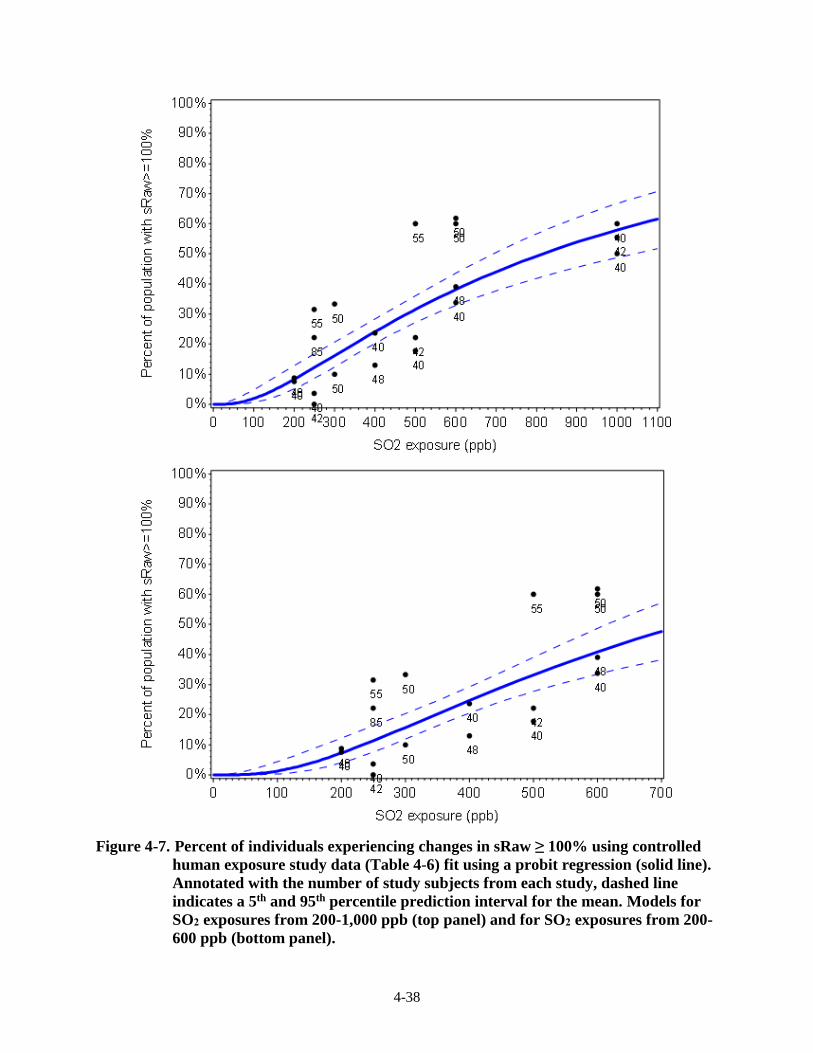
4-38
Figure 4-7. Percent of individuals experiencing changes in sRaw ≥ 100% using controlled
human exposure study data (Table 4-6) fit using a probit regression (solid line).
Annotated with the number of study subjects from each study, dashed line
indicates a 5th and 95th percentile prediction interval for the mean. Models for
SO2 exposures from 200-1,000 ppb (top panel) and for SO2 exposures from 200-
600 ppb (bottom panel).
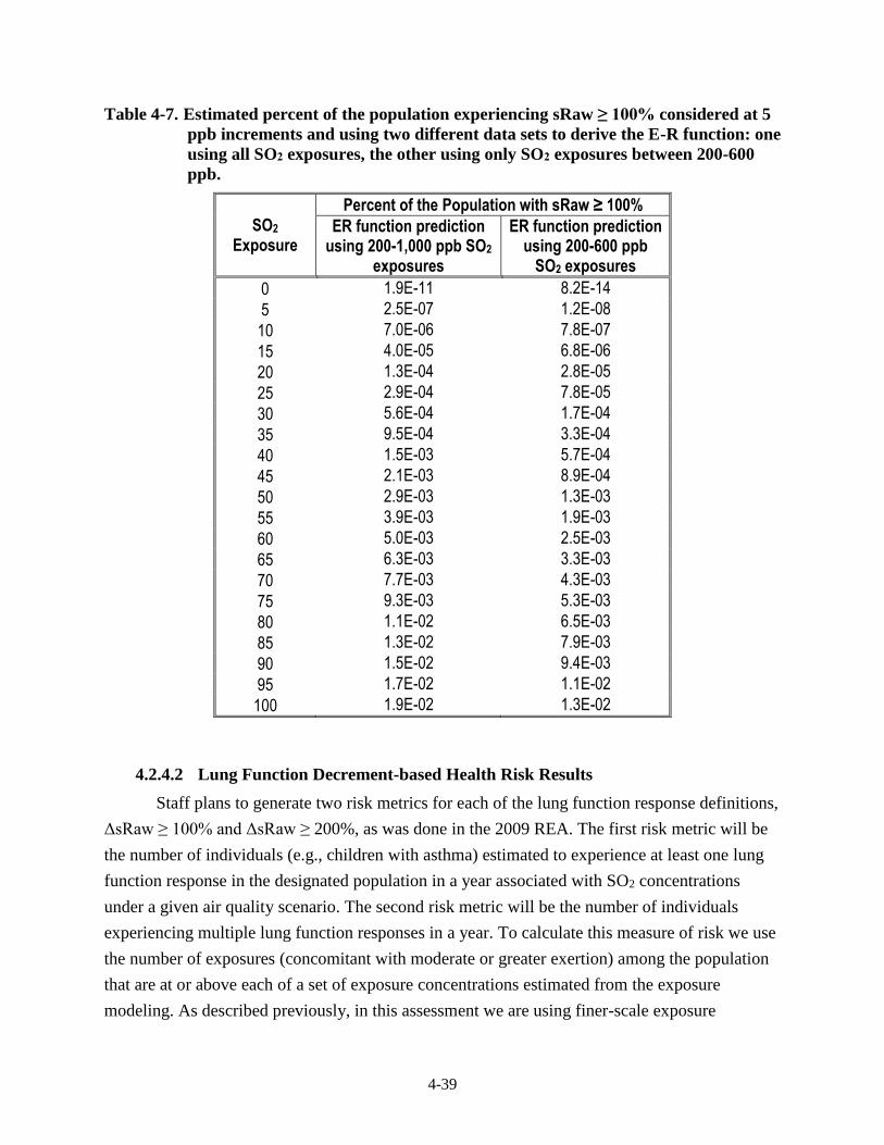
4-39
Table 4-7. Estimated percent of the population experiencing sRaw ≥ 100% considered at 5
ppb increments and using two different data sets to derive the E-R function: one
using all SO2 exposures, the other using only SO2 exposures between 200-600
ppb.
SO2 Exposure
Percent of the Population with sRaw ≥ 100%
ER function prediction using 200-1,000 ppb SO2
exposures
ER function prediction using 200-600 ppb
SO2 exposures
0 1.9E-11 8.2E-14
5 2.5E-07 1.2E-08
10 7.0E-06 7.8E-07
15 4.0E-05 6.8E-06
20 1.3E-04 2.8E-05
25 2.9E-04 7.8E-05
30 5.6E-04 1.7E-04
35 9.5E-04 3.3E-04
40 1.5E-03 5.7E-04
45 2.1E-03 8.9E-04
50 2.9E-03 1.3E-03
55 3.9E-03 1.9E-03
60 5.0E-03 2.5E-03
65 6.3E-03 3.3E-03
70 7.7E-03 4.3E-03
75 9.3E-03 5.3E-03
80 1.1E-02 6.5E-03
85 1.3E-02 7.9E-03
90 1.5E-02 9.4E-03
95 1.7E-02 1.1E-02
100 1.9E-02 1.3E-02
4.2.4.2 Lung Function Decrement-based Health Risk Results
Staff plans to generate two risk metrics for each of the lung function response definitions,
ΔsRaw ≥ 100% and ΔsRaw ≥ 200%, as was done in the 2009 REA. The first risk metric will be
the number of individuals (e.g., children with asthma) estimated to experience at least one lung
function response in the designated population in a year associated with SO2 concentrations
under a given air quality scenario. The second risk metric will be the number of individuals
experiencing multiple lung function responses in a year. To calculate this measure of risk we use
the number of exposures (concomitant with moderate or greater exertion) among the population
that are at or above each of a set of exposure concentrations estimated from the exposure
modeling. As described previously, in this assessment we are using finer-scale exposure
4-40
designations, particularly at exposures below 200 ppb, to better capture the variation that may
correspond to both the changes in the percent of individuals responding as well as the expected
variation occurring in number of individuals exposed from one exposure bin to another. For
exposures <150 ppb, the exposure bins will be set at 10 ppb increments (e.g., 10–20 ppb, 20–30
ppb, etc.), exposures ≥150 and <200 ppb will be at 20 ppb increments, exposures ≥200 and <300
ppb will be at 25 ppb increments, and exposures ≥300 ppb using 50 ppb increments. From this
we calculate the number of exposures within each exposure bin. We then calculate the number of
occurrences of lung function response by multiplying the number of exposures in an exposure
bin by the response probability (given by the probit E-R function for the specified definition of
lung function response) associated with the midpoint of that bin (e.g., the midpoint of the 10-20
ppb bin is 15 ppb, thus the frequency/probability obtained from the probit function at 15 ppb will
be used to estimate the number of persons responding). Results for all bins will be summed to
generate the total estimated risk. Additionally, because we will have the risk estimates
effectively apportioned to the exposure bins, the contribution to risk estimates from each
exposure bin will also be provided.
4.3 ASSESSMENT OF VARIABILITY AND CHARACTERIZATION OF
UNCERTAINTY
An important issue associated with any population exposure and risk assessment is the
assessment of variability and characterization of uncertainty. Variability refers to the inherent
heterogeneity in a population or variable of interest (e.g., residential air exchange rates). The
degree of variability cannot be reduced through further research, only better characterized with
additional measurement. Uncertainty refers to the lack of knowledge regarding the values of
model input variables (i.e., parameter uncertainty), the physical systems or relationships used
(i.e., use of input variables to estimate exposure or risk or model uncertainty), and in specifying
the scenario that is consistent with purpose of the assessment (i.e., scenario uncertainty).
Uncertainty is, ideally, reduced to the maximum extent possible through improved measurement
of key parameters and iterative model refinement. The following two sections describe the
approaches we will use to assess variability and to characterize uncertainty in this REA. The
primary outcome will be a summary of variability and uncertainty evaluations conducted to date
regarding our SO2 exposure assessments and APEX exposure modeling and to identify the most
important elements of uncertainty in need of further characterization. Each section will contain a
concise tabular summary of the identified components and how, for elements of uncertainty,
each source may affect the estimated exposures.
4-41
4.3.1 Assessment of Variability and Co-variability
The goal in addressing variability in the REA will be to ensure that the estimates of
exposure and risk reflect the variability of SO2 concentrations in ambient air, population
characteristics, associated SO2 exposures, physiological characteristics of simulated individuals,
and potential health risk across the study areas and for the simulated at-risk populations. In the
REA, there are several algorithms that we plan to use to account for variability of input data
when generating the number of estimated benchmark exceedances or health risk outputs. For
example, variability may arise from differences in the population residing within census tracts
(e.g., age distribution) and the activities that may affect population exposure to SO2 (e.g., time
spent outdoors, performing moderate or greater exertion level activities outdoors). A complete
range of potential exposure levels and associated risk estimates can be generated when
appropriately addressing variability in exposure and risk assessments; note however that the
range of values obtained would be within the constraints of the input parameters, algorithms, or
modeling system used, not necessarily the complete range of the true exposure or risk values.
We note also that correlations and non-linear relationships between variables input to the
model can result in the model producing inaccurate results if the inherent relationships between
these variables are not preserved. That is why APEX is also designed to account for co-
variability, or linear and nonlinear correlation among the model inputs, provided that enough is
known about these relationships to specify them. This is accomplished by providing inputs that
enable the correlation to be modeled explicitly within APEX. For example, there is a non-linear
relationship between the outdoor temperature and air exchange rate in homes. One factor that
contributes to this non-linear relationship is that windows tend to be closed more often when
temperatures are at either low or high extremes than when temperatures are moderate. This
relationship is explicitly modeled in APEX by specifying different probability distributions of air
exchange rates for different ambient air temperatures.
In any event, important sources of the variability and co-variability accounted for by
APEX and used for this SO2 exposure analysis will be identified and summarized. Where
possible, staff will identify and incorporate the observed variability in input data sets rather than
employing standard default assumptions and/or using point estimates to describe model inputs.
Where appropriate for this REA, we will begin with descriptions regarding variability
distributions used for the last O3 REA and also acknowledge particular variabilities associated
with some of the algorithms and processes in the version of APEX which we apply.
4.3.2 Characterization of Uncertainty
While it may be possible to capture a range of exposure or risk values by accounting for
variability inherent to influential factors, the true exposure or risk for any given individual within
4-42
a study area may be unknown, though can be estimated. To characterize health risks, exposure
and risk assessors commonly use an iterative process of gathering data, developing models, and
estimating exposures and risks, given the goals of the assessment, scale of the assessment
performed, and limitations of the input data available. However, significant uncertainty often
remains and emphasis is then placed on characterizing the nature of that uncertainty and its
impact on exposure and risk estimates.
Above we summarized the most important uncertainties potentially affecting the
exposure estimates reported in the 2009 REA and how we can address some of them using newly
available information. Additionally, the REAs conducted for the most recent NO2 (U.S. EPA,
2008), carbon monoxide (U.S. EPA, 2010), and O3 (U.S. EPA, 2014b) also characterized the
uncertainties associated with APEX exposure modeling (among other pollutant specific issues).
Conclusions drawn from each of these characterizations, and considering these in light of new
information and approaches used for the REA, and any new evaluations performed in the current
REA will be synthesized following the approach outlined by WHO (2008) and used to identify,
evaluate, and prioritize the most important uncertainties relevant to the estimated exposure and
risk outcomes. Staff plan to use a mainly qualitative approach supplemented by various model
sensitivity analyses and input data evaluations, all complementary to quantitative uncertainty
characterizations conducted for the 2007 O3 REA by Langstaff (2007).
The approach to be used here varies from that described by WHO (2008) in that a greater
focus will be placed on evaluating the direction and the magnitude59 of the uncertainty; that is,
qualitatively rating how the source of uncertainty, in the presence of alternative information, may
affect the estimated exposures and health risk results. Following the identification of key
uncertainties, staff will subjectively scale the overall impact of the uncertainty by considering the
relationship between the source of uncertainty and the exposure concentrations (e.g., low,
moderate, or high potential impact). Also to the extent possible, staff will also include an
assessment of the direction of influence, indicating how the source of uncertainty could affect
estimated exposures or risk estimates (e.g., the uncertainty could lead to over- or under-
estimates). Further, and consistent with the WHO (2008) guidance, staff will discuss the
uncertainty in the knowledge base (e.g., the accuracy of the data used, acknowledgement of data
gaps) and decisions made where possible (e.g., selection of particular model forms). The output
of the uncertainty characterization will be a summary describing, for each identified source of
uncertainty, the magnitude of the impact and the direction of influence the uncertainty may have
on the exposure and risk characterization results.
59 This is synonymous with the “level of uncertainty” discussed in WHO (2008), section 5.1.2.2.
4-43
The following summarizes two potential sensitivity analyses concerning input data,
output data, or model aspects that may, as feasible, be conducted in addition to the base level
analyses described above.
Because there is uncertainty in the risk estimated for exposures below 200 ppb and we
will have risk estimates associated with numerous exposure bins, we will present
complementary risk estimates that assume the particular contribution from an exposure
bin is negligible (e.g., assume a threshold at 10 ppb, such that for all people having their
daily maximum 5-minute exposure < 10 ppb, none will be estimated as having an sRaw
response of interest).
For the benchmark analysis and for identifying exposure bins used in the risk estimation,
exposures of interest are those that occur while at moderate or greater exertion (i.e., have
an EVR = 21 L/min-m2). There are a number of uncertainties associated with the
development of this threshold, including the estimation of body surface area and the
target ventilation rate. We plan to explore these and any other influential factors that
might influence this selected value, based on any relevant and available information in
the controlled exposure studies and other published studies.
4-44
REFERENCES
Bethel R, Erle D, Epstein J, Sheppard D, Nadel J, Boushey H. 1983. Effect of exercise rate and
route of inhalation on sulfur-dioxide induced- bronchoconstriction in asthmatic subjects.
American Review of Respiratory Disease. 128:592-596.
Bethel R, Sheppard D, Geffroy B, Tam E, Nadel J, Boushey H. 1985. Effect of 0.25 ppm sulfur
dioxide on airway resistance in freely breathing, heavily exercising, asthmatic subjects.
American Review of Respiratory Disease. 131:659-661.
Geyh AS, Xue J, Özkaynak H, Spengler JD. 2000. The Harvard Southern California chronic
ozone exposure study: assessing ozone exposure of grade-school-age children in two
Southern California communities. Environmental Health Perspectives. 108:265-270.
Glen G, Smith L, Isaacs K, McCurdy T, Langstaff J. 2008. A new method of longitudinal diary
assembly for human exposure modeling. Journal of Exposure Science and Environmental
Epidemiology. 18:299-311.
Kehrl H, Roger J, Hazucha M, Horstman D. 1987. Differing Response of asthmatics to sulfur
dioxide exposure with continuous and intermittent exercise. American Review of
Respiratory Disease. 135:350-355.
Langstaff JE. 2007. Analysis of Uncertainty in Ozone Population Exposure Modeling, OAQPS
Staff Memorandum to Ozone NAAQS Review, January 31. Washington, DC: Office of
Air Radiation. (EPA docket number OAR-2005-0172). Available at:
<http://www.epa.gov/ttn/naaqs/standards/ozone/s_O3_cr_td.html>
Linn WS, Avol EL, Shamoo DA, Venet TG, Anderson KR, Whynot JD, Hackney JD. 1984.
Asthmatics' responses to 6-hr sulfur dioxide exposures on two successive days. Archives
of Environmental Health. 39:313-319.
Linn W, Avol E, Peng R-C, Shamoo D, Hackney J. 1987. Replicated dose-response study of
sulfur dioxide effects in normal, atopic, and asthmatic volunteers. American Review of
Respiratory Disease. 136:1127-1134.
Linn W, Avol E, Shamoo D, Peng R-C, Spier C, Smith M, Hackney J. 1988. Effect of
metaproterenol sulfate on mild asthmatics' response to sulfur dioxide exposure and
exercise. Archives of Environmental Health. 43:399-406.
Linn W, Shamoo D, Peng RC, Clark K, Avol E, Hackney J. 1990. Responses to sulfur dioxide
and exercise by medication-dependent asthmatics: effect of varying medication levels.
Archives of Environmental Health. 45:24-30.
Rizzo M. 2009. Investigation of How Distributions of Hourly Sulfur Dioxide Concentrations
Have Changed Over Time in Six Cities. Sulfur Dioxide Review Docket. Docket ID No.
EPA-HQ-OAR-2007-0352. Available at: www.regulations.gov.
4-45
Roger L, Kehrl H, Hazucha M, and Horstman D. 1985. Bronchoconstriction in asthmatics
exposed to sulfur dioxide during repeated exercise. Journal of Applied Physiology.
59:784-791.
Samet J. 2009. Clean Air Scientific Advisory Committee’s (CASAC) Review of EPA's Risk and
Exposure Assessment (REA) to Support the Review of the SO2 Primary National
Ambient Air Quality Standards: Second Draft. EPA-CASAC-09-007. Available at:
https://www3.epa.gov/ttn/naaqs/standards/so2/s_so2_cr.html
U.S. EPA 1992. Protocol for Determining the Best Performing Model, EPA-454/R-92-025. U.S.
Environmental Protection Agency, Research Triangle Park, NC.
U.S. EPA. 1997. Exposure Factors Handbook (1997 Final Report). U.S. Environmental
Protection Agency, Washington, DC, EPA/600/P-95/002F a-c, 1997. Available at:
https://cfpub.epa.gov/si/si_public_record_report.cfm?dirEntryId=12464
U.S. EPA. 2008. Risk and Exposure Assessment to Support the Review of the NO2 Primary
National Ambient Air Quality Standard. Office of Air Quality Planning and Standards,
U.S. Environmental Protection Agency, Research Triangle Park, NC, 27711. EPA-452/R-
08-008a, 2008. Available at:
https://www3.epa.gov/ttn/naaqs/standards/no2so2sec/cr_rea.html
U.S. EPA. 2010. Quantitative Risk and Exposure Assessment for Carbon Monoxide - Amended.
Office of Air Quality Planning and Standards, U.S. Environmental Protection Agency,
Research Triangle Park, NC, 27711. EPA-452/R-10-006. Available at:
https://www.epa.gov/naaqs/carbon-monoxide-co-standards-risk-and-exposure-
assessments-current-review
U.S. EPA. 2011. Exposure Factors Handbook 2011 Edition (Final). U.S. Environmental
Protection Agency, Washington, DC, EPA/600/R-09/052F, 2011. Available at:
https://cfpub.epa.gov/ncea/risk/recordisplay.cfm?deid=236252
U.S. EPA. 2012a. Air Pollutants Exposure Model Documentation (APEX, Version 4.5)
Volume I: User’s Guide. Office of Air Quality Planning and Standards, U.S.
Environmental Protection Agency, Research Triangle Park, NC, 27711. EPA-452/B-17-
001a. Available at: https://www.epa.gov/fera/apex-user-guides
U.S. EPA. 2012b. Air Pollutants Exposure Model Documentation (APEX, Version 4.5)
Volume II: Technical Support Document. Office of Air Quality Planning and Standards,
U.S. Environmental Protection Agency, Research Triangle Park, NC, 27711. EPA-452/B-
17-001b. Available at: https://www.epa.gov/fera/apex-user-guides
U.S. EPA. 2014a. The Consolidated Human Activity Database – Master Version (CHAD-
Master). Technical Memorandum. U.S. Environmental Protection Agency, National
Exposure Research Laboratory, Research Triangle Park, NC, 27711. Updated
09/15/2014. Available at: https://www.epa.gov/healthresearch/consolidated-human-
activity-database-chad-use-human-exposure-and-health-studies-and
4-46
U.S. EPA. 2014b. Health Risk and Exposure Assessment for Ozone. Office of Air Quality
Planning and Standards, U.S. Environmental Protection Agency, Research Triangle Park,
NC, 27711. EPA-452/R-14-004a. Available at: https://www.epa.gov/naaqs/ozone-o3-
standards-risk-and-exposure-assessments-current-review
U.S. EPA. 2016. SO2 NAAQS Designations Modeling Technical Assistant Document – Draft.
Office of Air Quality Planning and Standards, U.S. Environmental Protection Agency,
Research Triangle Park, NC, 27711. August 2016. Available at:
https://www.epa.gov/sites/production/files/2016-06/documents/so2modelingtad.pdf
Whitfield R, Biller W, Jusko M, Keisler J. 1996. A Probabilistic Assessment of Health Risks
Associated with Short- and Long-Term Exposure to Tropospheric Ozone. Argonne, IL:
Argonne National Laboratory.
WHO. 2008. WHO/IPCS Harmonization Project Document No. 6. Part 1: Guidance Document
on Characterizing and Communicating Uncertainty in Exposure Assessment. Geneva,
World Health Organization, International Programme on Chemical Safety. Available at:
http://www.who.int/ipcs/methods/harmonization/areas/exposure/en/
Xue J, McCurdy T, Spengler J, and Özkaynak H. 2004. Understanding variability in time spent
in selected locations for 7-12 year old children. Journal of Exposure Analysis and
Environmental Epidemiology. 14:222-33.
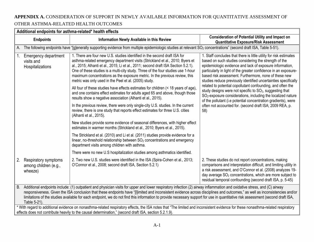
A-1
APPENDIX A. CONSIDERATION OF SUPPORT IN NEWLY AVAILABLE INFORMATION FOR QUANTITATIVE ASSESSMENT OF
OTHER ASTHMA-RELATED HEALTH OUTCOMES
Additional endpoints for asthma-related* health effects
Endpoints Information Newly Available in this Review Consideration of Potential Utility and Impact on
Quantitative Exposure/Risk Assessment
A. The following endpoints have “[g]enerally supporting evidence from multiple epidemiologic studies at relevant SO2 concentrations” (second draft ISA, Table 5-51).
1. Emergency department visits and Hospitalizations
1. There are four new U.S. studies identified in the second draft ISA for asthma-related emergency department visits (Strickland et al., 2010; Byers et al., 2015; Alhanti et al., 2015; Li et al., 2011; second draft ISA Section 5.2.1). One of these studies is a multi-city study. Three of the four studies use 1-hour maximum concentrations as the exposure metric. In the previous review, this metric was only used in the Peel et al. (2005) study.
All four of these studies have effects estimates for children (< 18 years of age), and one contains effect estimates for adults aged 65 and above, though those results show a negative association (Alhanti et al., 2015).
In the previous review, there were only single-city U.S. studies. In the current review, there is one study that reports effect estimates for three U.S. cities (Alhanti et al., 2015).
New studies provide some evidence of seasonal differences, with higher effect estimates in warmer months (Strickland et al., 2010; Byers et al., 2015).
The Strickland et al. (2010) and Li et al. (2011) studies provide evidence for a linear, no-threshold relationship between SO2 concentrations and emergency department visits among children with asthma.
There were no new U.S hospitalization studies among asthmatics identified.
1. Staff concludes that there is little utility for risk estimates based on such studies considering the strength of the epidemiologic evidence and lack of exposure information, particularly in light of the greater confidence in an exposure-based risk assessment. Furthermore, none of these new studies reduce previously identified uncertainties specifically related to potential copollutant confounding, and often the study designs were not specific to SO2, suggesting that SO2-exposure considerations, including the localized nature of the pollutant (i.e potential concentration gradients), were often not accounted for. (second draft ISA; 2009 REA, p. 58)
2. Respiratory symptoms among children (e.g., wheeze)
2. Two new U.S. studies were identified in the ISA (Spira-Cohen et al., 2013; O’Connor et al., 2008; second draft ISA, Section 5.2.1)
2. These studies do not report concentrations, making comparisons and interpretation difficult, and limiting utility in a risk assessment, and O’Connor et al. (2008) analyzes 19-day average SO2 concentrations, which are more subject to residual temporal confounding (second draft ISA, p. 5-45)
B. Additional endpoints include: (1) outpatient and physician visits for upper and lower respiratory infection (2) airway inflammation and oxidative stress, and (C) airway responsiveness. Given the ISA conclusion that these endpoints have “[l]imited and inconsistent evidence across disciplines and outcomes,” as well as inconsistencies and/or limitations of the studies available for each endpoint, we do not find this information to provide necessary support for use in quantitative risk assessment (second draft ISA, Table 5-21).
* With regard to additional evidence on nonasthma-related respiratory effects, the ISA notes that “The limited and inconsistent evidence for these nonasthma-related respiratory effects does not contribute heavily to the causal determination,” (second draft ISA, section 5.2.1.9).
A-2
REFERENCES
Alhanti, BA; Chang, HH; Winquist, A; Mulholland, JA; Darrow, LA; Sarnat, SE. (2016).
Ambient air pollution and emergency department visits for asthma: A multi-city
assessment of effect modification by age. J Expo Sci Environ Epidemiol 26: 180-188.
http://dx.doi.org/10.1038/jes.2015.57
Byers, N; Ritchey, M; Vaidyanathan, A; Brandt, AJ; Yip, F. (2015). Short-term effects of
ambient air pollutants on asthma-related emergency department visits in Indianapolis,
Indiana, 2007-2011. J Asthma 53: 1-8.
http://dx.doi.org/10.3109/02770903.2015.1091006
Li, S; Batterman, S; Wasilevich, E; Wahl, R; Wirth, J; Su, FC; Mukherjee, B. (2011).
Association of daily asthma emergency department visits and hospital admissions with
ambient air pollutants among the pediatric Medicaid population in Detroit: Time-series
and time-stratified case-crossover analyses with threshold effects. Environ Res 111:
1137-1147. http://dx.doi.org/10.1016/j.envres.2011.06.002
Peel, JL; Tolbert, PE; Klein, M; Metzger, KB; Flanders, WD; Todd, K; Mulholland, JA; Ryan,
PB; Frumkin, H. (2005). Ambient air pollution and respiratory emergency department
visits. Epidemiology 16: 164-174.
http://dx.doi.org/10.1097/01.ede.0000152905.42113.db
O'Connor, GT; Neas, L; Vaughn, B; Kattan, M; Mitchell, H; Crain, EF; Evans, R, III; Gruchalla,
R; Morgan, W; Stout, J; Adams, GK; Lippmann, M. (2008). Acute respiratory health
effects of air pollution on children with asthma in US inner cities. J Allergy Clin
Immunol 121: 1133-1139.e1131. http://dx.doi.org/10.1016/j.jaci.2008.02.020
Strickland, MJ; Darrow, LA; Klein, M; Flanders, WD; Sarnat, JA; Waller, LA; Sarnat, SE;
Mulholland, JA; Tolbert, PE. (2010). Short-term associations between ambient air
pollutants and pediatric asthma emergency department visits. Am J Respir Crit Care Med
182: 307-316. http://dx.doi.org/10.1164/rccm.200908-1201OC
Spira-Cohen, A; Chen, LC; Kendall, M; Lall, R; Thurston, GD. (2011). Personal exposures to
traffic-related air pollution and acute respiratory health among Bronx schoolchildren with
asthma. Environ Health Perspect 119: 559-565.
http://dx.doi.org/10.1289/ehp.1002653
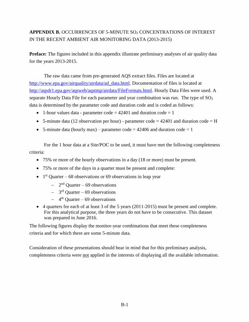
B-1
APPENDIX B. OCCURRENCES OF 5-MINUTE SO2 CONCENTRATIONS OF INTEREST
IN THE RECENT AMBIENT AIR MONITORING DATA (2013-2015)
Preface: The figures included in this appendix illustrate preliminary analyses of air quality data
for the years 2013-2015.
The raw data came from pre-generated AQS extract files. Files are located at
http://www.epa.gov/airquality/airdata/ad_data.html. Documentation of files is located at
http://aqsdr1.epa.gov/aqsweb/aqstmp/airdata/FileFormats.html. Hourly Data Files were used. A
separate Hourly Data File for each parameter and year combination was run. The type of SO2
data is determined by the parameter code and duration code and is coded as follows:
1-hour values data - parameter code = 42401 and duration code = 1
5-minute data (12 observation per hour) - parameter code = 42401 and duration code = H
5-minute data (hourly max) – parameter code = 42406 and duration code = 1
For the 1 hour data at a Site/POC to be used, it must have met the following completeness
criteria:
75% or more of the hourly observations in a day (18 or more) must be present.
75% or more of the days in a quarter must be present and complete:
1st Quarter – 68 observations or 69 observations in leap year
2nd Quarter – 69 observations
3rd Quarter – 69 observations
4th Quarter – 69 observations
4 quarters for each of at least 3 of the 5 years (2011-2015) must be present and complete.
For this analytical purpose, the three years do not have to be consecutive. This dataset
was prepared in June 2016.
The following figures display the monitor-year combinations that meet these completeness
criteria and for which there are some 5-minute data.
Consideration of these presentations should bear in mind that for this preliminary analysis,
completeness criteria were not applied in the interests of displaying all the available information.
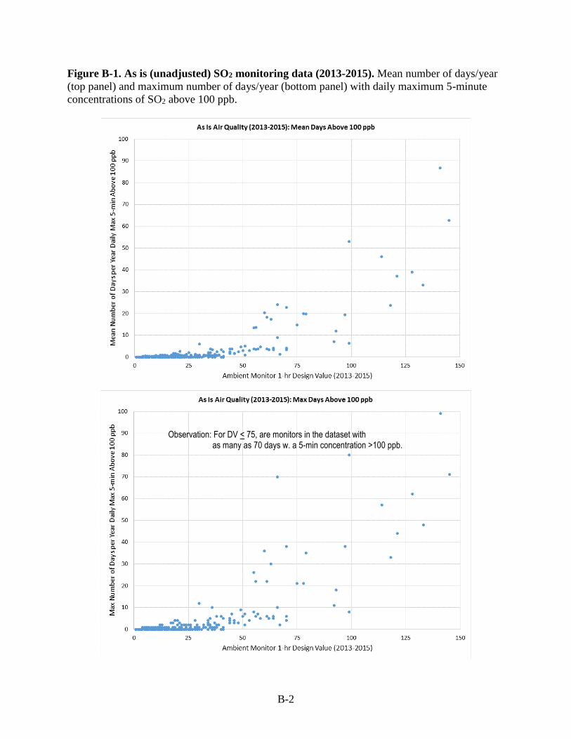
B-2
Figure B-1. As is (unadjusted) SO2 monitoring data (2013-2015). Mean number of days/year
(top panel) and maximum number of days/year (bottom panel) with daily maximum 5-minute
concentrations of SO2 above 100 ppb.
Observation: For DV < 75, are monitors in the dataset with as many as 70 days w. a 5-min concentration >100 ppb.
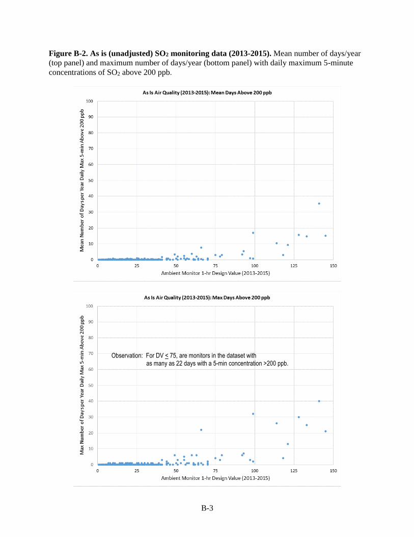
B-3
Figure B-2. As is (unadjusted) SO2 monitoring data (2013-2015). Mean number of days/year
(top panel) and maximum number of days/year (bottom panel) with daily maximum 5-minute
concentrations of SO2 above 200 ppb.
Observation: For DV < 75, are monitors in the dataset with as many as 22 days with a 5-min concentration >200 ppb.
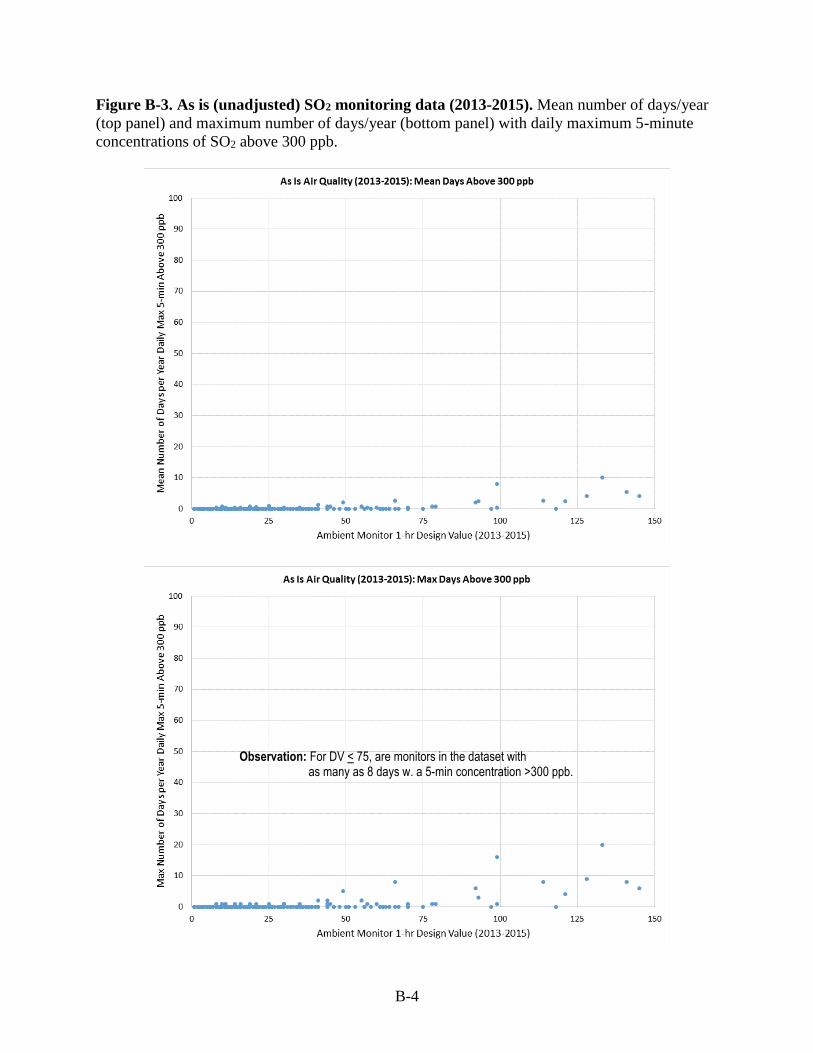
B-4
Figure B-3. As is (unadjusted) SO2 monitoring data (2013-2015). Mean number of days/year
(top panel) and maximum number of days/year (bottom panel) with daily maximum 5-minute
concentrations of SO2 above 300 ppb.
Observation: For DV < 75, are monitors in the dataset with as many as 8 days w. a 5-min concentration >300 ppb.
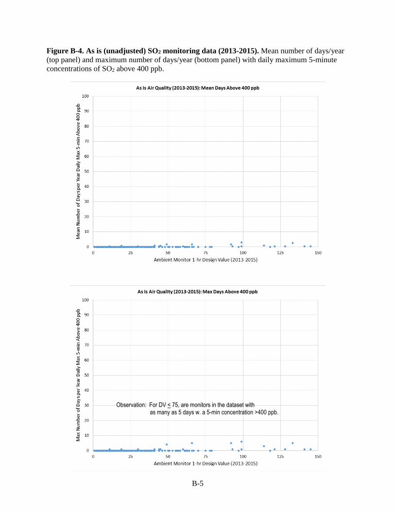
B-5
Figure B-4. As is (unadjusted) SO2 monitoring data (2013-2015). Mean number of days/year
(top panel) and maximum number of days/year (bottom panel) with daily maximum 5-minute
concentrations of SO2 above 400 ppb.
Observation: For DV < 75, are monitors in the dataset with as many as 5 days w. a 5-min concentration >400 ppb.
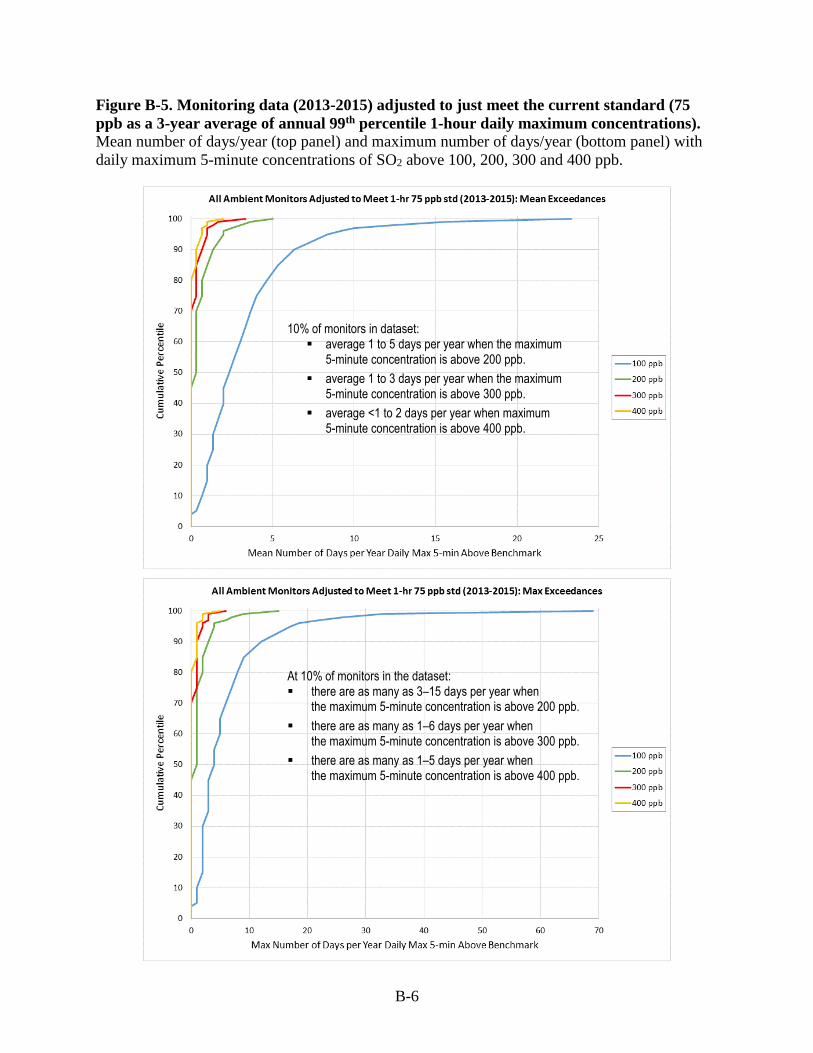
B-6
Figure B-5. Monitoring data (2013-2015) adjusted to just meet the current standard (75
ppb as a 3-year average of annual 99th percentile 1-hour daily maximum concentrations). Mean number of days/year (top panel) and maximum number of days/year (bottom panel) with
daily maximum 5-minute concentrations of SO2 above 100, 200, 300 and 400 ppb.
10% of monitors in dataset: average 1 to 5 days per year when the maximum
5-minute concentration is above 200 ppb.
average 1 to 3 days per year when the maximum 5-minute concentration is above 300 ppb.
average <1 to 2 days per year when maximum 5-minute concentration is above 400 ppb.
At 10% of monitors in the dataset: there are as many as 3–15 days per year when
the maximum 5-minute concentration is above 200 ppb.
there are as many as 1–6 days per year when the maximum 5-minute concentration is above 300 ppb.
there are as many as 1–5 days per year when the maximum 5-minute concentration is above 400 ppb.
C-1
APPENDIX C. COMPARISONS OF SO2 HOURLY CONCENTRATION DISTRIBUTIONS
BETWEEN HIGH AND LOW YEARS IN 2011-2015
Preface: The figures included in this appendix illustrate preliminary analyses of air quality data
for the years 2011-2015.
The figures below represent the analyses of recent air quality data to evaluate the
appropriateness of the proportional adjustment approach used in the 2009 REA. As described in
section 4.1.3.4, the figures below are the results for the monitors in the potential study areas that
did not have the highest design value during the 2011-2015 period. The figures below compare
the monitoring data for a low concentration year with a data for a high concentration year, with
low and high defined by having a design value that is either below (a low year) or above (a high
year) the level of the existing standard (99th percentile daily maximum 1-hour of 75 ppb).
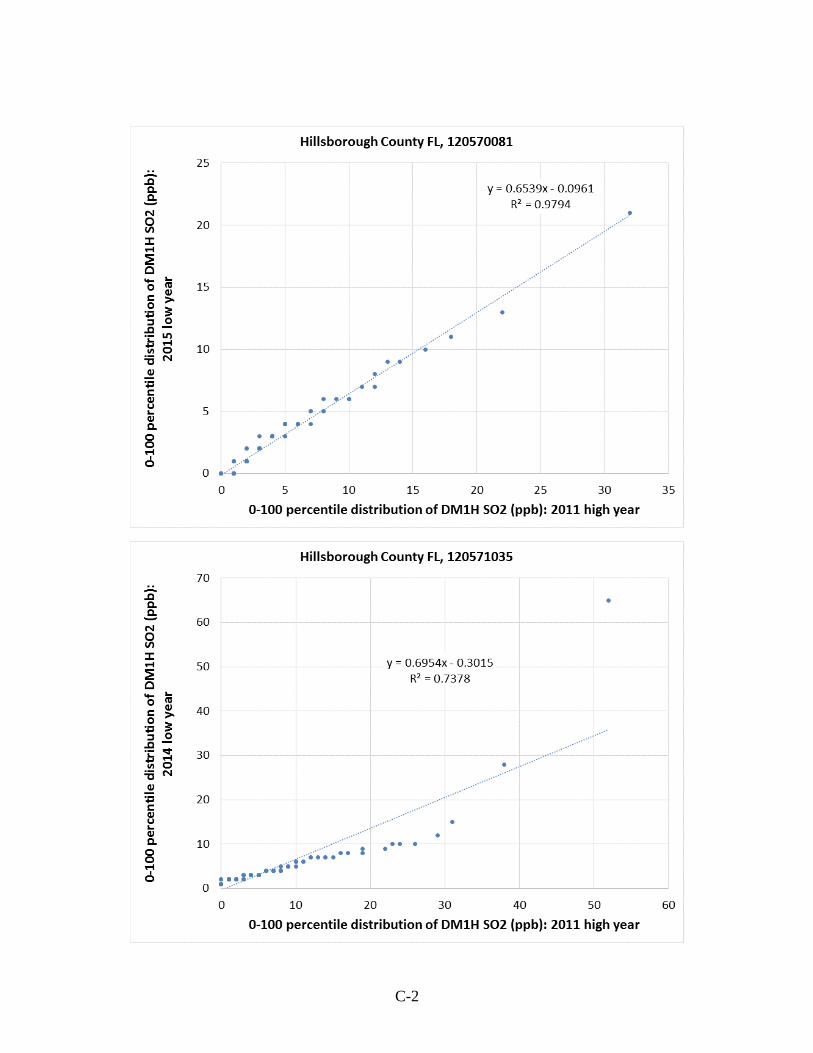
C-2
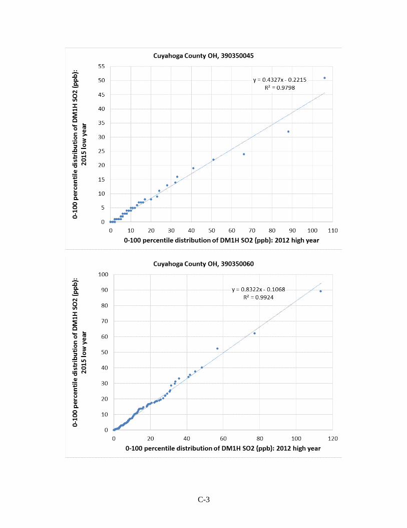
C-3
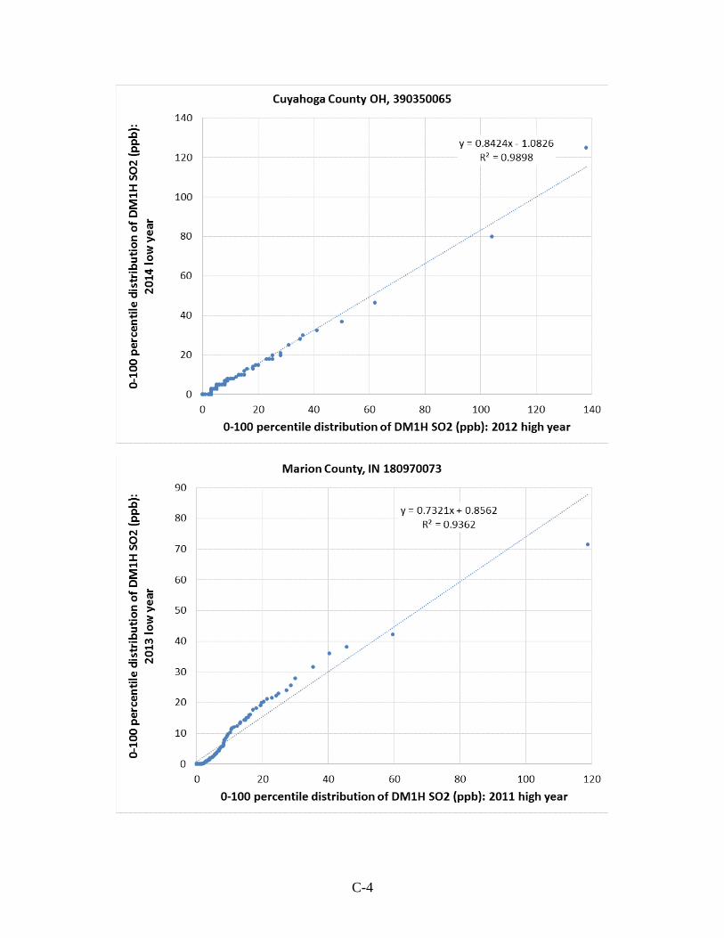
C-4

C-5
United States
Environmental Protection
Agency
Office of Air Quality Planning and Standards
Health and Environmental Impacts Division
Research Triangle Park, NC
Publication No. EPA-452/P-17-001
February 2017