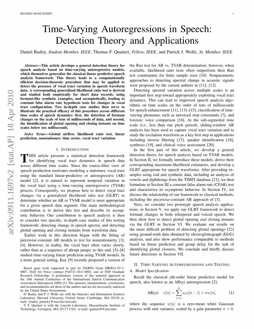
REVISED MANUSCRIPT 1

Time-Varying Autoregressions in Speech:Detection Theory and Applications

Daniel Rudoy, Student Member, IEEE, Thomas F. Quatieri, Fellow, IEEE, and Patrick J. Wolfe, Sr. Member, IEEE

Abstract—This article develops a general detection theory forspeech analysis based on time-varying autoregressive models,which themselves generalize the classical linear predictive speechanalysis framework. This theory leads to a computationallyefficient decision-theoretic procedure that may be applied todetect the presence of vocal tract variation in speech waveformdata. A corresponding generalized likelihood ratio test is derivedand studied both empirically for short data records, usingformant-like synthetic examples, and asymptotically, leading toconstant false alarm rate hypothesis tests for changes in vocaltract configuration. Two in-depth case studies then serve toillustrate the practical efficacy of this procedure across differenttime scales of speech dynamics: first, the detection of formantchanges on the scale of tens of milliseconds of data, and second,the identification of glottal opening and closing instants on timescales below ten milliseconds.

Index Terms—Glottal airflow, likelihood ratio test, linearprediction, nonstationary time series, vocal tract variation

I. INTRODUCTION

THIS article presents a statistical detection frameworkfor identifying vocal tract dynamics in speech data

across different time scales. Since the source-filter view ofspeech production motivates modeling a stationary vocal tractusing the standard linear-predictive or autoregressive (AR)model [2], it is natural to represent temporal variation inthe vocal tract using a time-varying autoregressive (TVAR)process. Consequently, we propose here to detect vocal tractchanges via a generalized likelihood ratio test (GLRT) todetermine whether an AR or TVAR model is most appropriatefor a given speech data segment. Our main methodologicalcontribution is to derive this test and describe its asymp-totic behavior. Our contribution to speech analysis is thento consider two specific, in-depth case studies of this testingframework: detecting change in speech spectra, and detectingglottal opening and closing instants from waveform data.

Earlier work in this direction began with the fitting ofpiecewise-constant AR models to test for nonstationarity [3],[4]. However, in reality, the vocal tract often varies slowly,rather than as a sequence of abrupt jumps; to this end, [5]–[8]studied time-varying linear prediction using TVAR models. Ina more general setting, Kay [9] recently proposed a version of

Based upon work supported in part by DARPA Grant HR0011-07-1-0007, DoD Air Force contract FA8721-10-C-0002, and an NSF GraduateResearch Fellowship. A preliminary version of this material appeared inthe 10th Annual Conference of the International Speech CommunicationAssociation (Interspeech 2009) [1]. The opinions, interpretations, conclusions,and recommendations are those of the authors and are not necessarily endorsedby the United States Government.

D. Rudoy and P. J. Wolfe are with the Statistics and Information SciencesLaboratory, Harvard University, Oxford Street, Cambridge, MA 02138 (e-mail: {rudoy, patrick}@seas.harvard.edu)

T. F. Quatieri is with the Lincoln Laboratory, Massachusetts Institute ofTechnology, Lexington, MA 02173 USA. (e-mail: quatieri@ll.mit.edu).

the Rao test for AR vs. TVAR determination; however, whenavailable, likelihood ratio tests often outperform their Raotest counterparts for finite sample sizes [10]. Nonparametricapproaches to detecting spectral change in acoustic signalswere proposed by the current authors in [11], [12].

Detecting spectral variation across multiple scales is animportant first step toward appropriately exploiting vocal tractdynamics. This can lead to improved speech analysis algo-rithms on time scales on the order of tens of millisecondsfor speech enhancement [11], [13]–[15], classification of time-varying phonemes such as unvoiced stop consonants [7], andforensic voice comparison [16]. At the sub-segmental timescale (i.e., less than one pitch period), sliding-window ARanalysis has been used to capture vocal tract variation and tostudy the excitation waveform as a key first step in applicationsincluding inverse filtering [17], speaker identification [18],synthesis [19], and clinical voice assessment [20].

In the first part of this article, we develop a generaldetection theory for speech analysis based on TVAR models.In Section II, we formally introduce these models, derive theircorresponding maximum-likelihood estimators, and develop aGLRT appropriate for speech waveforms. After providing ex-amples using real and synthetic data, including an analysis ofvowels and diphthongs from the TIMIT database [21], we thenformulate in Section III a constant false alarm rate (CFAR) testand characterize its asymptotic behavior. In Section IV, wediscuss the relationship of our framework to classical methods,including the piecewise-constant AR approach of [3].

Next, we consider two prototype speech analysis applica-tions: in Section V, we apply our GLRT framework to detectformant changes in both whispered and voiced speech. Wethen show how to detect glottal opening and closing instantsvia the GLRT in Section VI. We evaluate our results onthe more difficult problem of detecting glottal openings [22]using ground-truth data obtained by electroglottograph (EGG)analysis, and also show performance comparable to methodsbased on linear prediction and group delay for the task ofidentifying glottal closures. We conclude and briefly discussfuture directions in Section VII.

II. TIME-VARYING AUTOREGRESSIONS AND TESTING

A. Model Specification

Recall the classical pth-order linear predictive model forspeech, also known as an AR(p) autoregression [2]:

AR(p): x[n] =

p∑i=1

aix[n− i] + σw[n], (1)

where the sequence w[n] is a zero-mean white Gaussianprocess with unit variance, scaled by a gain parameter σ > 0.

arX

iv:0

911.

1697

v2 [

stat

.AP]

18

Apr

201

0

REVISED MANUSCRIPT 2

A more flexible pth-order time-varying autoregressive modelis given by the following discrete-time difference equation [5]:

TVAR(p): x[n] =

p∑i=1

ai[n]x[n− i] + σw[n]. (2)

In contrast to (1), the linear prediction coefficients ai[n] of (2)are time-dependent, implying a nonstationary random process.

The model of (2) requires specification of precisely how thelinear prediction coefficients evolve in time. Here we chooseto expand them in a set of q+1 basis functions fj [n] weighedby coefficients αij as follows:

ai[n] =

q∑j=0

αijfj [n], for all 1 ≤ i ≤ p. (3)

We assume throughout that the “constant” function f0[n] = 1is included in the chosen basis set, so that the classical AR(p)model of (1) is recovered as ai ≡ αi0 · 1 whenever αij = 0for all j > 0. Many choices are possible for the functionsfj [n]—Legendre [23] and Fourier [5] polynomials, discreteprolate spheroidal functions [6], and even wavelets [24] havebeen used in speech applications.

The functional expansion of (3) was first studied in [23],[25], and subsequently applied to speech analysis by [5]–[7],among others. Coefficient trajectories ai[n] have also beenmodeled as sample paths of a suitably chosen stochastic pro-cess (see, e.g., [26]). In this case, however, estimation typicallyrequires stochastic filtering [13] or iterative methods [27] incontrast to the least-squares estimators available for the modelof (3), which are described in Section II-C below.

B. AR vs. TVAR Generalized Likelihood Ratio Test (GLRT)We now describe how to test the hypothesis H0 that a

given signal segment x = (x[0] x[1] · · · x[N−1])T has beengenerated by an AR(p) process according to (1), against thealternative hypothesis H1 of a TVAR(p) process as specifiedby (2) and (3) above. We introduce a GLRT to examineevidence of change in linear prediction coefficients over time,and consequently in the vocal tract resonances that theyrepresent in the classical source-filter model of speech.

According to the functional expansion of (3), the TVAR(p)model of (2) is fully described by p(q + 1) expansion coeffi-cients αij and the gain term σ. For convenience we group thecoefficients αij into q + 1 vectors αj , 0 ≤ j ≤ q, as

αj ,(α1j α2j · · · αpj

)T.

We may then partition a vector α ∈ Rp(q+1)×1 into blocksassociated to the AR(p) portion of the model αAR, and theremainder αTV, which captures time variation:

α ,(αTAR | αTTV

)T=(αT0 | αT1 αT2 · · · αTq

)T. (4)

Recalling that the TVAR(p) model (hypothesis H1) reducesto an AR(p) model (hypothesis H0) precisely when αj = 0for all j > 0, we may formulate the following hypothesis test:

Model : TVAR(p) with parameters α, σ2;

Hypotheses :

{H0 : αj = 0 for all j > 0,H1 : αj 6= 0 for at least one j > 0.

(5)

Estimate αTV, αARunder H1

Estimate, αARunder H0

x

Estimate σ2

under H1

Estimate σ2

under H0

T(x)-

+

( )1

2ˆ( ) ln HN p σ−

( )0

2ˆ( ) ln HN p σ−

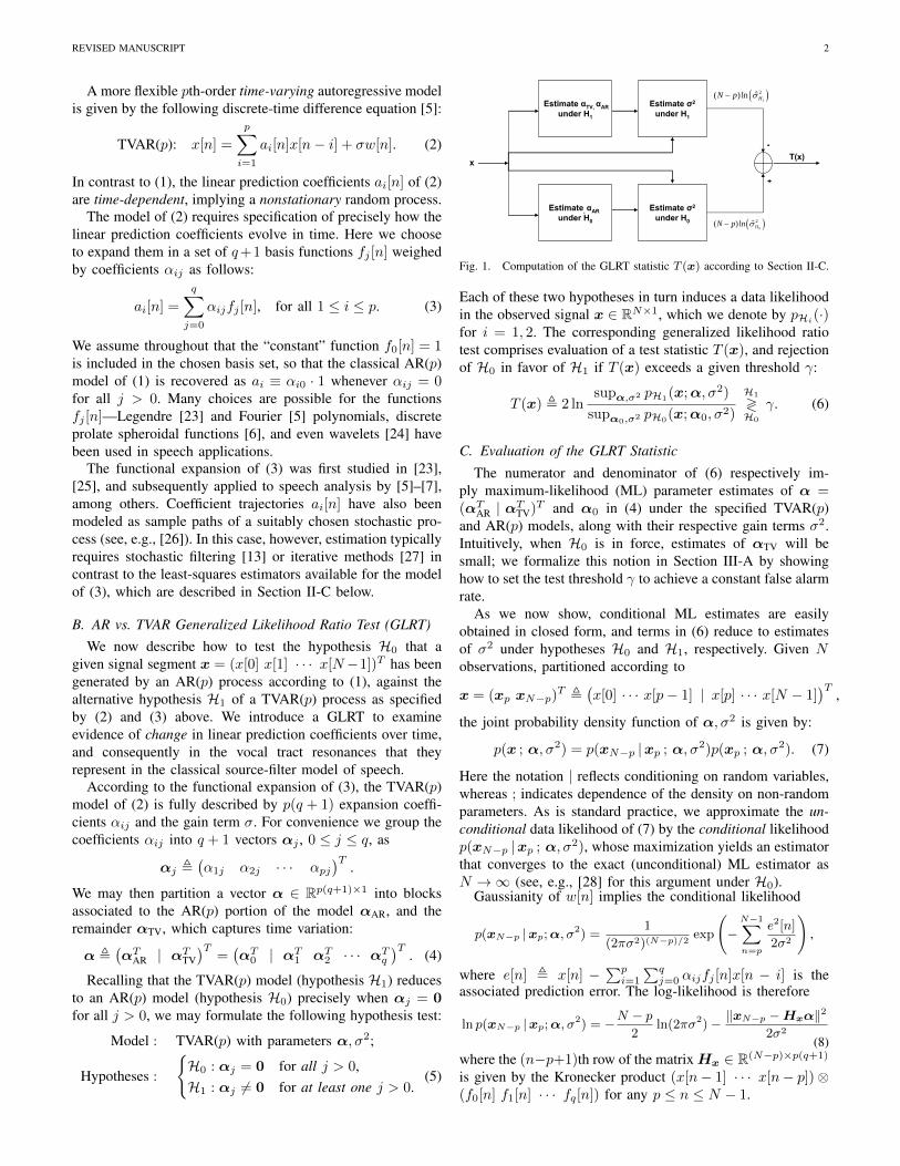
Fig. 1. Computation of the GLRT statistic T (x) according to Section II-C.

Each of these two hypotheses in turn induces a data likelihoodin the observed signal x ∈ RN×1, which we denote by pHi

(·)for i = 1, 2. The corresponding generalized likelihood ratiotest comprises evaluation of a test statistic T (x), and rejectionof H0 in favor of H1 if T (x) exceeds a given threshold γ:

T (x) , 2 lnsupα,σ2 pH1

(x;α, σ2)

supα0,σ2 pH0(x;α0, σ2)

H1

≷H0

γ. (6)

C. Evaluation of the GLRT Statistic

The numerator and denominator of (6) respectively im-ply maximum-likelihood (ML) parameter estimates of α =(αTAR | αTTV)

T and α0 in (4) under the specified TVAR(p)and AR(p) models, along with their respective gain terms σ2.Intuitively, when H0 is in force, estimates of αTV will besmall; we formalize this notion in Section III-A by showinghow to set the test threshold γ to achieve a constant false alarmrate.

As we now show, conditional ML estimates are easilyobtained in closed form, and terms in (6) reduce to estimatesof σ2 under hypotheses H0 and H1, respectively. Given Nobservations, partitioned according to

x = (xp xN−p)T ,

(x[0] · · · x[p− 1] | x[p] · · · x[N − 1]

)T,

the joint probability density function of α, σ2 is given by:

p(x ; α, σ2) = p(xN−p |xp ; α, σ2)p(xp ; α, σ2). (7)

Here the notation | reflects conditioning on random variables,whereas ; indicates dependence of the density on non-randomparameters. As is standard practice, we approximate the un-conditional data likelihood of (7) by the conditional likelihoodp(xN−p |xp ; α, σ2), whose maximization yields an estimatorthat converges to the exact (unconditional) ML estimator asN →∞ (see, e.g., [28] for this argument under H0).

Gaussianity of w[n] implies the conditional likelihood

p(xN−p |xp;α, σ2) =

1

(2πσ2)(N−p)/2exp

(−

N−1∑n=p

e2[n]

2σ2

),

where e[n] , x[n] −∑pi=1

∑qj=0 αijfj [n]x[n − i] is the

associated prediction error. The log-likelihood is therefore

ln p(xN−p |xp;α, σ2) = −N − p

2ln(2πσ2)− ‖xN−p −Hxα‖2

2σ2

(8)where the (n−p+1)th row of the matrixHx ∈ R(N−p)×p(q+1)

is given by the Kronecker product (x[n− 1] · · · x[n− p])⊗(f0[n] f1[n] · · · fq[n]) for any p ≤ n ≤ N − 1.

REVISED MANUSCRIPT 3

100 200 300 400 500−4

−2

0

2

4Synthetic Signal

x[n]

Sample Number100 200 300 400 500

−1.5

−1

−0.5

0

0.5

1True AR Trajectories

a[n]

Sample Number

100 200 300 400 500−1.5

−1

−0.5

0

0.5

1

Sample Number

Coe

ffici

ent M

agni

tude

Fitted AR Trajectories

True modelFitted AR modelFitted TVAR model

−1 −0.5 0 0.5 1

−1

−0.5

0

0.5

1

Imag

inar

y A

xis

Real Axis

Pole Trajectories

0 0.2 0.4 0.6 0.8 10

0.2

0.4

0.6

0.8

1

Pro

bab

ility

of

Det

ecti

on

Frequency Jump: π/80 rad

5ms10ms15ms20ms

0 0.2 0.4 0.6 0.8 10

0.2

0.4

0.6

0.8

1Frequency Jump: 3π/80 rad

5ms10ms15ms20ms

0 0.2 0.4 0.6 0.8 10

0.2

0.4

0.6

0.8

1Frequency Jump: 5π/80 rad

5ms10ms15ms20ms

0 0.2 0.4 0.6 0.8 10

0.2

0.4

0.6

0.8

1

Probability of False Alarm

Frequency Jump: 7π/80 rad

5ms10ms15ms20ms

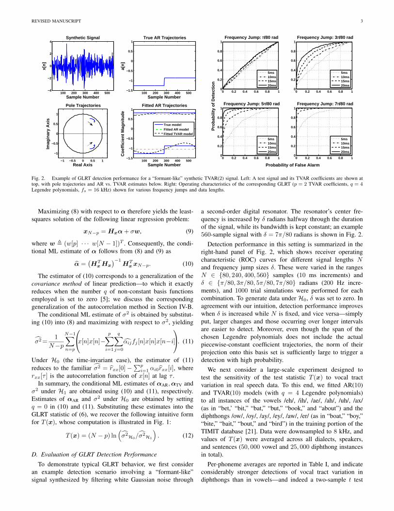
Fig. 2. Example of GLRT detection performance for a “formant-like” synthetic TVAR(2) signal. Left: A test signal and its TVAR coefficients are shown attop, with pole trajectories and AR vs. TVAR estimates below. Right: Operating characteristics of the corresponding GLRT (p = 2 TVAR coefficients, q = 4Legendre polynomials, fs = 16 kHz) shown for various frequency jumps and data lengths.

Maximizing (8) with respect to α therefore yields the least-squares solution of the following linear regression problem:

xN−p =Hxα+ σw, (9)

where w , (w[p] · · · w[N − 1])T . Consequently, the condi-tional ML estimate of α follows from (8) and (9) as

α =(HTxHx

)−1HTxxN−p. (10)

The estimator of (10) corresponds to a generalization of thecovariance method of linear prediction—to which it exactlyreduces when the number q of non-constant basis functionsemployed is set to zero [5]; we discuss the correspondinggeneralization of the autocorrelation method in Section IV-B.

The conditional ML estimate of σ2 is obtained by substitut-ing (10) into (8) and maximizing with respect to σ2, yielding

σ2=1

N−p

N−1∑n=p

x[n]x[n]− p∑i=1

q∑j=0

αijfj [n]x[n]x[n−i]

. (11)

Under H0 (the time-invariant case), the estimator of (11)reduces to the familiar σ2 = rxx[0] −

∑pi=1 αi0rxx[i], where

rxx[τ ] is the autocorrelation function of x[n] at lag τ .In summary, the conditional ML estimates of αAR,αTV and

σ2 under H1 are obtained using (10) and (11), respectively.Estimates of αAR and σ2 under H0 are obtained by settingq = 0 in (10) and (11). Substituting these estimates into theGLRT statistic of (6), we recover the following intuitive formfor T (x), whose computation is illustrated in Fig. 1:

T (x) = (N − p) ln(σ2H0/σ

2H1

). (12)

D. Evaluation of GLRT Detection Performance

To demonstrate typical GLRT behavior, we first consideran example detection scenario involving a “formant-like”signal synthesized by filtering white Gaussian noise through

a second-order digital resonator. The resonator’s center fre-quency is increased by δ radians halfway through the durationof the signal, while its bandwidth is kept constant; an example560-sample signal with δ = 7π/80 radians is shown in Fig. 2.

Detection performance in this setting is summarized in theright-hand panel of Fig. 2, which shows receiver operatingcharacteristic (ROC) curves for different signal lengths Nand frequency jump sizes δ. These were varied in the rangesN ∈ {80, 240, 400, 560} samples (10 ms increments) andδ ∈ {π/80, 3π/80, 5π/80, 7π/80} radians (200 Hz incre-ments), and 1000 trial simulations were performed for eachcombination. To generate data under H0, δ was set to zero. Inagreement with our intuition, detection performance improveswhen δ is increased while N is fixed, and vice versa—simplyput, larger changes and those occurring over longer intervalsare easier to detect. Moreover, even though the span of thechosen Legendre polynomials does not include the actualpiecewise-constant coefficient trajectories, the norm of theirprojection onto this basis set is sufficiently large to trigger adetection with high probability.

We next consider a large-scale experiment designed totest the sensitivity of the test statistic T (x) to vocal tractvariation in real speech data. To this end, we fitted AR(10)and TVAR(10) models (with q = 4 Legendre polynomials)to all instances of the vowels /eh/, /ih/, /ae/, /ah/, /uh/, /ax/(as in “bet,’ “bit,” “bat,” “but,” “book,” and “about”) and thediphthongs /ow/, /oy/, /ay/, /ey/, /aw/, /er/ (as in “boat,” “boy,”“bite,” “bait,” “bout,” and “bird”) in the training portion of theTIMIT database [21]. Data were downsampled to 8 kHz, andvalues of T (x) were averaged across all dialects, speakers,and sentences (50, 000 vowel and 25, 000 diphthong instancesin total).

Per-phoneme averages are reported in Table I, and indicateconsiderably stronger detections of vocal tract variation indiphthongs than in vowels—and indeed a two-sample t test

REVISED MANUSCRIPT 4

TABLE IVOCAL TRACT VARIATION IN TIMIT VOWELS & DIPHTHONGS.

Vowel eh ih ae ah uh axT (x) 67.5 60.5 94.6 63.8 58.9 32.1

Diphthong ow oy ay ey aw erT (x) 134.1 302.4 187.4 130.6 161.6 133.0

easily rejects (p-value u 0) the hypothesis that the averagevalues of T (x) for the two groups are equal. This findingis consistent with the physiology of speech production, anddemonstrates the sensitivity of the GLRT in practice.

III. ANALYSIS OF DETECTION PERFORMANCE

To apply the hypothesis test of (5), it is necessary to selecta threshold γ as per (6), such that the null hypothesis of abest-fit AR(p) model is rejected in favor of the fitted TVAR(p)model whenever T (x) > γ. Below we describe how to chooseγ to guarantee a constant false alarm rate (CFAR) for largesample sizes, and give the asymptotic (in N ) distribution of theGLRT statistic under H0 and H1, showing how these resultsyield practical consequences for speech analysis.

A. Derivation of GLRT Asymptotics and CFAR Test

Under suitable technical conditions [29], likelihood ratiostatistics take on a chi-squared distribution χ2

d(0) as the samplesize N grows large whenever H0 is in force, with the degreesof freedom d equal to the number of parameters restrictedunder the null hypothesis. In our setting, d = pq since the pqcoefficients αTV are restricted to be zero under H0, and wemay write that T (x) ∼ χ2

pq(0) under H0 as N →∞.Thus, we may specify an allowable asymptotic constant

false alarm rate for the GLRT of (5), defined as follows:

limN→∞

Pr {T (x) > γ;H0} = Pr{χ2pq(0) > γ

}. (13)

Since the asymptotic distribution of T (x) under H0 dependsonly on p and q, which are set in advance, we can determine aCFAR threshold γ by fixing a desired value (say, 5%) for theright-hand side of (13), and evaluating the inverse cumulativedistribution function of χ2

pq(0) to obtain the value of γ thatguarantees the specified (asymptotic) constant false alarm rate.

When x is a TVAR process so that the alternate hypothesisH1 is in force, T (x) instead takes on (as N → ∞) anoncentral chi-squared distribution χ2

d(λ). Its noncentralityparameter λ > 0 depends on the true but unknown parametersof the model under H1; thus in general

T (x)N→∞∼ χ2

pq(λ),

{λ = 0 under H0,λ > 0 under H1.

(14)

It is easily shown by the method of [9] that the expression forλ in the case at hand is given by

λ = αTTV(FTF ⊗ σ−2R)αTV, (15)

where · denotes the Schur complement with respect tothe first p × p matrix block of its argument, the (j + 1)th

column of the matrix F ∈ R(N−p)×(q+1) is given by(fj [p] fj [p+ 1] · · · fj [N − 1]

)T, and R is given by:

R ,

rxx[0] rxx[1] · · · rxx[p− 1]rxx[1] rxx[0] · · · rxx[p− 2]

......

. . ....

rxx[p− 1] rxx[p− 2] · · · rxx[0]

.

Here {rxx[0], rxx[1], . . . , rxx[p − 1]} is the autocorrelationsequence corresponding to αAR (given, e.g., by the “step-downalgorithm” [28]). The expression of (15) follows from thefact that F TF ⊗ σ−2R is the Fisher information matrix forour TVAR(p) model; its Schur complement arises from thecomposite form of our hypothesis test, since the parametersαAR, σ

2 are unrestricted under H0.More generally, we may relate this result to the underlying

TVAR coefficient trajectories ai[n], arranged as columns ofa matrix A, with each column-wise mean trajectory value acorresponding entry in a matrix A. Letting A , A−A denotethe centered columns of A, and noting both that F TF ⊗R =F TF ⊗ R and that F (F TF )−1F TA = A when H1 is inforce, properties of Kronecker products [30] can be used toshow that (15) may be written as

λ = σ−2 tr(ARAT ). (16)

Thus λ depends on the centered columns of A, which containthe true but unknown coefficient trajectories ai[n] minus theirrespective mean values.

B. Model Order Selection

The above results yield not only a practical CFARthreshold-setting procedure, but also a full asymptotic descrip-tion of the GLRT statistic of (6) under both H0 and H1. Inlight of this analysis, it is natural to ask how the TVAR modelorder p should be chosen in practice, along with the numberq of non-constant basis functions. In deference to the largeliterature on the former subject [2], we adopt here the standard“2 coefficients per 1 kHz of speech bandwidth” rule of thumb.

Intuitively, the choice of basis functions should be wellmatched to the expected characteristics of the coefficient tra-jectories ai[n]. To make this notion quantitatively precise, weappeal to the results of (14)–(16) as follows. First, the statis-tical power of our test to successfully detect small departuresfrom stationarity is measured by the quantity Pr

{χ2d(λ) > γ

}.

A result of [31] then shows that for fixed γ, the power functionPr{χ2d(λ) > γ

}is:

1) Strictly monotonically increasing in λ, for fixed d;2) Strictly monotonically decreasing in d for fixed λ.

Each of these properties in turn yields a direct and importantconsequence for speech analysis:• Test power is maximized when λ attains its largest value:

For fixed p and q, the noncentrality parameter λ of (16)determines the power of the test as a function of σ2 andthe true but unknown coefficient trajectories A.

• Overfitting the data reduces test power: Choosing p orq to be larger than the true data-generating model will

REVISED MANUSCRIPT 5

0 0.2 0.4 0.6 0.8 10.2

0.3

0.4

0.5

0.6

0.7

0.8

0.9

1

Probability of False Alarm

Pro

bab

ility

of

Det

ecti

on

Effect of Model Order on Detection Performance

p = 2p = 4p = 6p = 10

0 0.2 0.4 0.6 0.8 10.2

0.3

0.4

0.5

0.6

0.7

0.8

0.9

1

q = 1q = 4q = 7q = 10

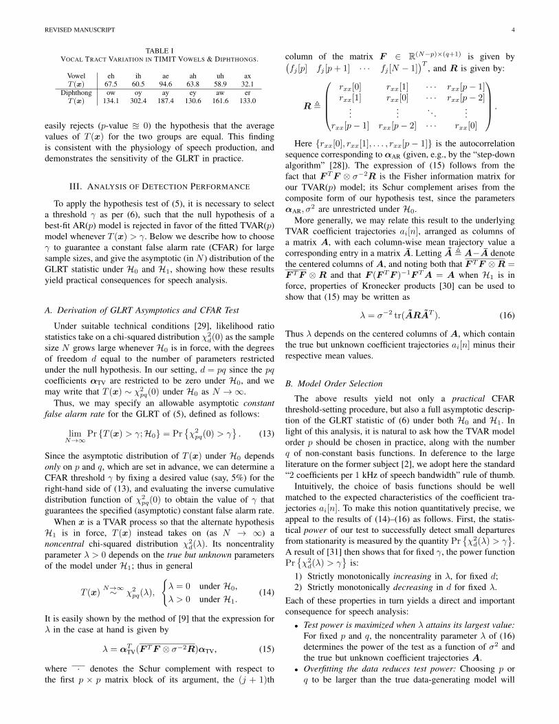
Fig. 3. The effect of overfitting on the detection performance of the GLRTstatistic for the synthetic signal of Fig. 2. An increase in the model order—p(left) and q (right)—decreases the probability of detection at any CFAR level.

result in a quantifiable loss in power, as λ will remainfixed while the degrees of freedom increase.

The first of these consequences follows from Property 1above, and reveals how test power depends on the energyof the centered TVAR trajectories A = A − A for fixedA and p, q, σ2. To verify the second consequence, observethat the product ARAT remains unaffected by an increase ineither p or q beyond that of the true TVAR(p) model. Thenby Property 2, the corresponding increase in the degrees offreedom pq will lead to a loss of test power.

This analysis implies that care should be taken to ade-quately capture the energy of TVAR coefficient trajectorieswhile guarding against overfitting; this formalizes our ear-lier intuition and reinforces the importance of choosing arelatively low-dimensional subspace formed by the span oflow-frequency basis functions whose degree of smoothnessis matched to the expected TVAR(p) signal characteristicsunder H1. This conclusion is further illustrated in Fig. 3,which considers the effects of overfitting on the “formant-like”synthetic example of Section II-D, with p = 2, N = 100 sam-ples, δ = 7π/80 radians, and piecewise-constant coefficienttrajectories. Not only is the effect of overfitting p apparent inthe left-hand panel, but the detection performance also suffersas the degree q of the Legendre polynomial basis is increased,as shown in the right-hand panel.

IV. RELATIONSHIP TO CLASSICAL APPROACHES

We now relate our hypothesis testing framework to twoclassical approaches in the literature. First, we compare itsperformance to that of Brandt’s test [3], which has seen wideuse both in earlier [4], [32] and more recent studies [15],[33], [34], for purposes of transient detection and automaticsegmentation for speech recognition and synthesis. Second,we demonstrate its advantages relative to the autocorrelationmethod of time-varying linear prediction [5], showing that datawindowing can adversely affect detection performance in thisnonstationary setting.

A. Classical Piecewise-Constant AR Approach

A related previous approach is to model x as an ARprocess with piecewise-constant parameters that can undergo

0 0.2 0.4 0.6 0.8 10

0.2

0.4

0.6

0.8

1

Pro

babi

lity

of D

etec

tion

Piecewise−Constant Signal ROCs

T’r(x)

T(x)

T’(x)

0 0.2 0.4 0.6 0.8 10

0.2

0.4

0.6

0.8

1

Probability of False Alarm

Piecewise−Linear Signal ROCs

T(x)

T’(x)

0 50 100 150 200 250 3002000

2100

2200

2300

2400

2500

ω[n

]

Time−Varying Center Frequency

0 50 100 150 200 2500

0.2

0.4

0.6

0.8

1

argm

axr T

’ r(x)

Sample Number

ML Changepoint Location

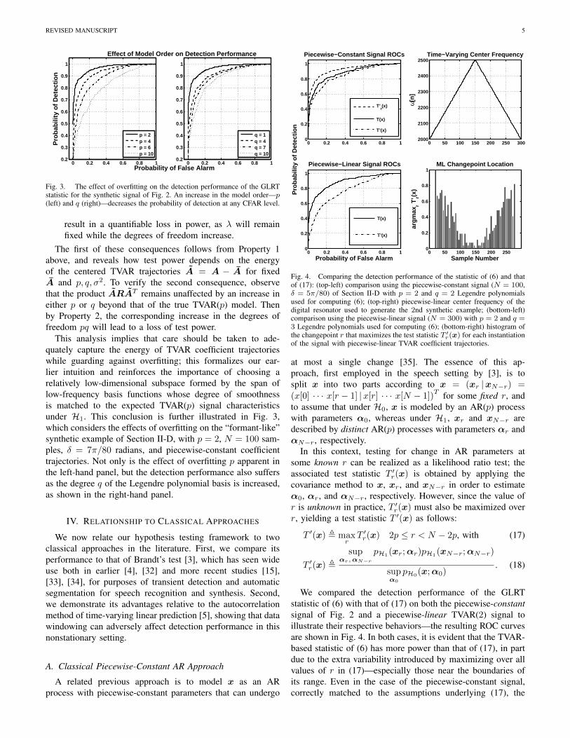
Fig. 4. Comparing the detection performance of the statistic of (6) and thatof (17): (top-left) comparison using the piecewise-constant signal (N = 100,δ = 5π/80) of Section II-D with p = 2 and q = 2 Legendre polynomialsused for computing (6); (top-right) piecewise-linear center frequency of thedigital resonator used to generate the 2nd synthetic example; (bottom-left)comparison using the piecewise-linear signal (N = 300) with p = 2 and q =3 Legendre polynomials used for computing (6); (bottom-right) histogram ofthe changepoint r that maximizes the test statistic T ′r(x) for each instantiationof the signal with piecewise-linear TVAR coefficient trajectories.

at most a single change [35]. The essence of this ap-proach, first employed in the speech setting by [3], is tosplit x into two parts according to x = (xr |xN−r) =(x[0] · · · x[r − 1] |x[r] · · · x[N − 1])

T for some fixed r, andto assume that under H0, x is modeled by an AR(p) processwith parameters α0, whereas under H1, xr and xN−r aredescribed by distinct AR(p) processes with parameters αr andαN−r, respectively.

In this context, testing for change in AR parameters atsome known r can be realized as a likelihood ratio test; theassociated test statistic T ′r(x) is obtained by applying thecovariance method to x, xr, and xN−r in order to estimateα0, αr, and αN−r, respectively. However, since the value ofr is unknown in practice, T ′r(x) must also be maximized overr, yielding a test statistic T ′(x) as follows:

T ′(x) , maxrT ′r(x) 2p ≤ r < N − 2p, with (17)

T ′r(x) ,

supαr,αN−r

pH1(xr;αr)pH1

(xN−r;αN−r)

supα0

pH0(x;α0). (18)

We compared the detection performance of the GLRTstatistic of (6) with that of (17) on both the piecewise-constantsignal of Fig. 2 and a piecewise-linear TVAR(2) signal toillustrate their respective behaviors—the resulting ROC curvesare shown in Fig. 4. In both cases, it is evident that the TVAR-based statistic of (6) has more power than that of (17), in partdue to the extra variability introduced by maximizing over allvalues of r in (17)—especially those near the boundaries ofits range. Even in the case of the piecewise-constant signal,correctly matched to the assumptions underlying (17), the

REVISED MANUSCRIPT 6

TVAR-based test is outperformed only when r is known apriori, and (18) is used. This effect is particularly acute in thesmall sample size setting—an important consideration for thesingle-pitch-period case study of Section VI.

This example demonstrates that any estimates of r can bemisleading under model mismatch. As shown in the bottom-right panel of Fig. 4, the detected changepoint is often esti-mated to be near the start or end of the data segment, butno “true” changepoint exists since the time-varying centerfrequency is continuously changing. Thus piecewise-constantmodels are only simple approximations to potentially complexTVAR coefficient dynamics; in contrast, flexibility in thechoice of basis functions implies applicability to a broaderclass of time-varying signals.

Note also that computing (17) requires brute-force evalua-tion of (18) for all values of r, whereas (6) need be calculatedonce. Moreover, T ′(x) fails to yield chi-squared (or anyclosed-form) asymptotics [35], thus precluding the design ofa CFAR test and any quantitative evaluation of test power.

B. Classical Linear Prediction and Windowing

Recall that our GLRT formulation of Section II, stemmingfrom the TVAR model of (2), generalized the covariancemethod of linear prediction to the time-varying setting. Theclassical autocorrelation method also yields least-squares esti-mators, but under a different error minimization criterion thanthat corresponding to conditional maximum likelihood. To seethis, consider the TVAR model

x[n] =

p∑i=1

ai[n− i]x[n− i] + σw[n], (19)

in lieu of (2). Grouping the coefficients αij into p vectors αi ,(αi0 αi1 · · · αiq)T , 1 ≤ i ≤ p, induces a partition of theexpansion coefficients given by α , (αT1 α

T2 · · · αTp )T—

a permutation of elements of α in (4). The autocorrelationestimator of α is then obtained by minimizing the predictionerror over all n ∈ Z, while assuming that x[n] = 0 for all n /∈[0, . . . , N − 1], and is equivalent to the least-squares solutionof the following linear regression problem:

x = Hxα+ σw, (20)

where w =(w[0] · · · w[N − 1])T

)and the nth row of

Hx ∈ RN×p(q+1) is given by (f0[n− 1]x[n− 1] · · · f0[n−p]x[n− p] · · · fq[n− 1]x[n− 1] · · · fq[n− p]x[n− p]). Theautocorrelation estimate of α then follows from (20) as:1α = (HT

x Hx)−1HT

xx. (21)

Moreover, when the autocorrelation method is used forspectral estimation in the stationary setting, x is often pre-multiplied by a smooth window. To empirically examinethe role of data windowing in the time-varying setting, wegenerated a short 196-sample synthetic TVAR(2) signal x

1As noted by [5], HTx Hx is a block-Toeplitz matrix comprised of p2

symmetric blocks of size (q+1)× (q+1)—this special structure arises as adirect consequence of the synchronous form of the TVAR trajectories in (19).Thus, the multichannel Levinson-Durbin recursion [36] may be used to invertHT

x Hx directly.

0 0.1 0.2 0.3 0.4 0.5 0.6 0.7 0.8 0.9 10

0.2

0.4

0.6

0.8

1

Probability of False Alarm

Pro

babi

lity

of D

etec

tion

Covariance−Based TestAutocorrelation−Based TestAutcorrelation (Hamming Window)

0 5 10 15 20 25 300

0.02

0.04

0.06

0.08

His

togr

am o

f T(x

)

T(x)

Autocorrelation−Based TestAutocorrelation (Hamming Window)

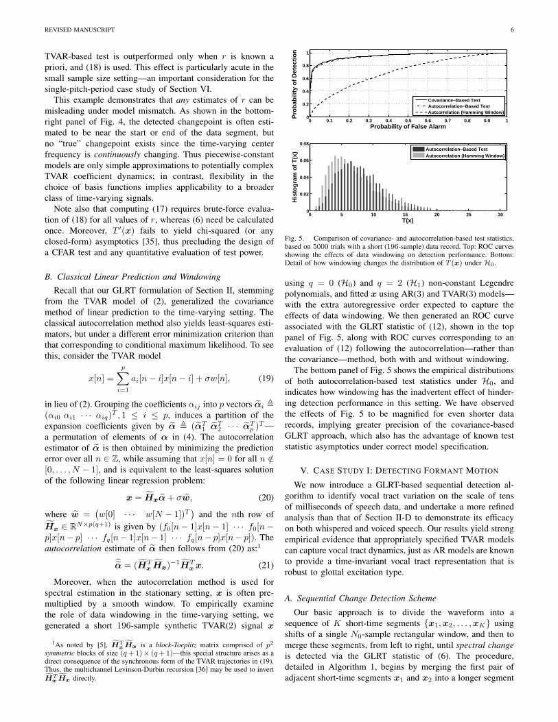
Fig. 5. Comparison of covariance- and autocorrelation-based test statistics,based on 5000 trials with a short (196-sample) data record. Top: ROC curvesshowing the effects of data windowing on detection performance. Bottom:Detail of how windowing changes the distribution of T (x) under H0.

using q = 0 (H0) and q = 2 (H1) non-constant Legendrepolynomials, and fitted x using AR(3) and TVAR(3) models—with the extra autoregressive order expected to capture theeffects of data windowing. We then generated an ROC curveassociated with the GLRT statistic of (12), shown in the toppanel of Fig. 5, along with ROC curves corresponding to anevaluation of (12) following the autocorrelation—rather thanthe covariance—method, both with and without windowing.

The bottom panel of Fig. 5 shows the empirical distributionsof both autocorrelation-based test statistics under H0, andindicates how windowing has the inadvertent effect of hinder-ing detection performance in this setting. We have observedthe effects of Fig. 5 to be magnified for even shorter datarecords, implying greater precision of the covariance-basedGLRT approach, which also has the advantage of known teststatistic asymptotics under correct model specification.

V. CASE STUDY I: DETECTING FORMANT MOTION

We now introduce a GLRT-based sequential detection al-gorithm to identify vocal tract variation on the scale of tensof milliseconds of speech data, and undertake a more refinedanalysis than that of Section II-D to demonstrate its efficacyon both whispered and voiced speech. Our results yield strongempirical evidence that appropriately specified TVAR modelscan capture vocal tract dynamics, just as AR models are knownto provide a time-invariant vocal tract representation that isrobust to glottal excitation type.

A. Sequential Change Detection Scheme

Our basic approach is to divide the waveform into asequence of K short-time segments {x1,x2, . . . ,xK} usingshifts of a single N0-sample rectangular window, and then tomerge these segments, from left to right, until spectral changeis detected via the GLRT statistic of (6). The procedure,detailed in Algorithm 1, begins by merging the first pair ofadjacent short-time segments x1 and x2 into a longer segment

REVISED MANUSCRIPT 7

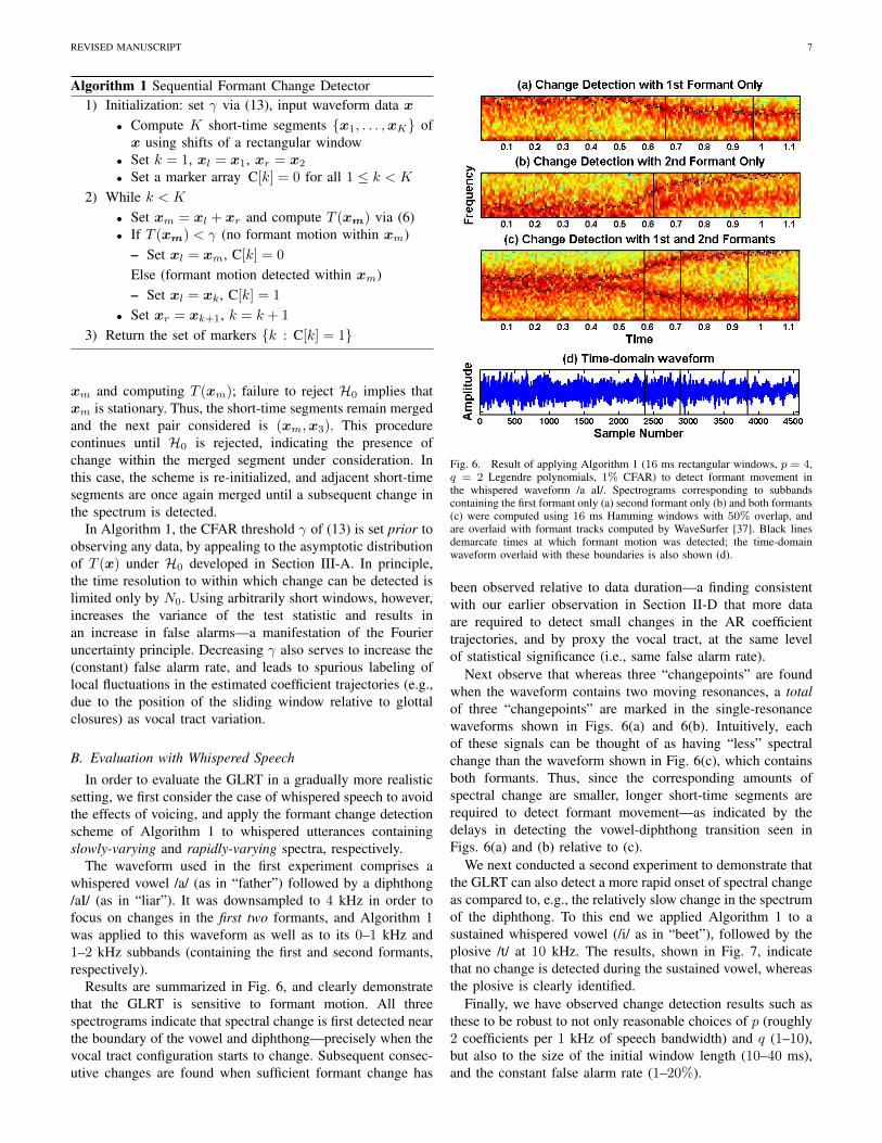
Algorithm 1 Sequential Formant Change Detector1) Initialization: set γ via (13), input waveform data x

• Compute K short-time segments {x1, . . . ,xK} ofx using shifts of a rectangular window

• Set k = 1, xl = x1, xr = x2

• Set a marker array C[k] = 0 for all 1 ≤ k < K

2) While k < K

• Set xm = xl + xr and compute T (xm) via (6)• If T (xm) < γ (no formant motion within xm)

– Set xl = xm, C[k] = 0

Else (formant motion detected within xm)– Set xl = xk, C[k] = 1

• Set xr = xk+1, k = k + 1

3) Return the set of markers {k : C[k] = 1}

xm and computing T (xm); failure to reject H0 implies thatxm is stationary. Thus, the short-time segments remain mergedand the next pair considered is (xm,x3). This procedurecontinues until H0 is rejected, indicating the presence ofchange within the merged segment under consideration. Inthis case, the scheme is re-initialized, and adjacent short-timesegments are once again merged until a subsequent change inthe spectrum is detected.

In Algorithm 1, the CFAR threshold γ of (13) is set prior toobserving any data, by appealing to the asymptotic distributionof T (x) under H0 developed in Section III-A. In principle,the time resolution to within which change can be detected islimited only by N0. Using arbitrarily short windows, however,increases the variance of the test statistic and results inan increase in false alarms—a manifestation of the Fourieruncertainty principle. Decreasing γ also serves to increase the(constant) false alarm rate, and leads to spurious labeling oflocal fluctuations in the estimated coefficient trajectories (e.g.,due to the position of the sliding window relative to glottalclosures) as vocal tract variation.

B. Evaluation with Whispered Speech

In order to evaluate the GLRT in a gradually more realisticsetting, we first consider the case of whispered speech to avoidthe effects of voicing, and apply the formant change detectionscheme of Algorithm 1 to whispered utterances containingslowly-varying and rapidly-varying spectra, respectively.

The waveform used in the first experiment comprises awhispered vowel /a/ (as in “father”) followed by a diphthong/aI/ (as in “liar”). It was downsampled to 4 kHz in order tofocus on changes in the first two formants, and Algorithm 1was applied to this waveform as well as to its 0–1 kHz and1–2 kHz subbands (containing the first and second formants,respectively).

Results are summarized in Fig. 6, and clearly demonstratethat the GLRT is sensitive to formant motion. All threespectrograms indicate that spectral change is first detected nearthe boundary of the vowel and diphthong—precisely when thevocal tract configuration starts to change. Subsequent consec-utive changes are found when sufficient formant change has

Fig. 6. Result of applying Algorithm 1 (16 ms rectangular windows, p = 4,q = 2 Legendre polynomials, 1% CFAR) to detect formant movement inthe whispered waveform /a aI/. Spectrograms corresponding to subbandscontaining the first formant only (a) second formant only (b) and both formants(c) were computed using 16 ms Hamming windows with 50% overlap, andare overlaid with formant tracks computed by WaveSurfer [37]. Black linesdemarcate times at which formant motion was detected; the time-domainwaveform overlaid with these boundaries is also shown (d).

been observed relative to data duration—a finding consistentwith our earlier observation in Section II-D that more dataare required to detect small changes in the AR coefficienttrajectories, and by proxy the vocal tract, at the same levelof statistical significance (i.e., same false alarm rate).

Next observe that whereas three “changepoints” are foundwhen the waveform contains two moving resonances, a totalof three “changepoints” are marked in the single-resonancewaveforms shown in Figs. 6(a) and 6(b). Intuitively, eachof these signals can be thought of as having “less” spectralchange than the waveform shown in Fig. 6(c), which containsboth formants. Thus, since the corresponding amounts ofspectral change are smaller, longer short-time segments arerequired to detect formant movement—as indicated by thedelays in detecting the vowel-diphthong transition seen inFigs. 6(a) and (b) relative to (c).

We next conducted a second experiment to demonstrate thatthe GLRT can also detect a more rapid onset of spectral changeas compared to, e.g., the relatively slow change in the spectrumof the diphthong. To this end we applied Algorithm 1 to asustained whispered vowel (/i/ as in “beet”), followed by theplosive /t/ at 10 kHz. The results, shown in Fig. 7, indicatethat no change is detected during the sustained vowel, whereasthe plosive is clearly identified.

Finally, we have observed change detection results such asthese to be robust to not only reasonable choices of p (roughly2 coefficients per 1 kHz of speech bandwidth) and q (1–10),but also to the size of the initial window length (10–40 ms),and the constant false alarm rate (1–20%).

REVISED MANUSCRIPT 8

0.05 0.1 0.15 0.2 0.25 0.3 0.35 0.4 0.45

Spectrogram

Time

Fre

quen

cy

0 500 1000 1500 2000 2500 3000 3500 4000 4500

Time−domain waveform

Sample Number

Am

plitu

de

Fig. 7. Algorithm 1 (16 ms windows, p=10, q=4 Legendre polynomials,1% CFAR), applied to detect formant movement in the whispered waveform/i t/. Its spectrogram (top) is overlaid with formant tracks computed byWaveSurfer [37] and black lines demarcating the time instants at whichformant motion was detected; the time-domain signal is also shown (bottom).

C. Extension to Voiced Speech

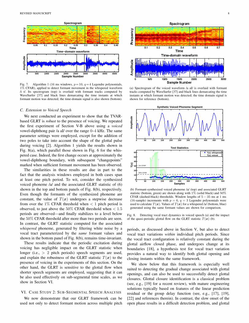
We next conducted an experiment to show that the TVAR-based GLRT is robust to the presence of voicing. We repeatedthe first experiment of Section V-B above using a voicedvowel-diphthong pair /a aI/ over the range 0–4 kHz. The sameparameter settings were employed, except for the addition oftwo poles to take into account the shape of the glottal pulseduring voicing [2]. Algorithm 1 yields the results shown inFig. 8(a), which parallel those shown in Fig. 6 for the whis-pered case. Indeed, the first change occurs at approximately thevowel-diphthong boundary, with subsequent “changepoints”marked when sufficient formant movement has been observed.

The similarities in these results are due in part to thefact that the analysis windows employed in both cases spanat least one pitch period. To wit, consider the synthesizedvoiced phoneme /a/ and the associated GLRT statistic of (6)shown in the top and bottom panels of Fig. 8(b), respectively.Even though the formants of the synthesized phoneme areconstant, the value of T (x) undergoes a stepwise decreasefrom over the 1% CFAR threshold when < 1 pitch period isobserved, to just above the 50% CFAR threshold when < 1.5periods are observed—and finally stabilizes to a level belowthe 50% CFAR threshold after more than two periods are seen.In contrast, the GLRT statistic computed for the associatedwhispered phoneme, generated by filtering white noise by avocal tract parameterized by the same formant values andshown in the bottom panel of Fig. 8(b), remains time-invariant.

These results indicate that the periodic excitation duringvoicing has negligible impact on the GLRT statistic whenlonger (i.e., > 2 pitch periods) speech segments are used,and explain the robustness of the GLRT statistic T (x) to thepresence of voicing in the experiments of this section. On theother hand, the GLRT is sensitive to the glottal flow whenshorter speech segments are employed, suggesting that it canbe also used effectively on sub-segmental time scales, as weshow in Section VI.

VI. CASE STUDY 2: SUB-SEGMENTAL SPEECH ANALYSIS

We now demonstrate that our GLRT framework can beused not only to detect formant motion across multiple pitch

(a) Spectrogram of the voiced waveform /a aI/ is overlaid with formanttracks computed by WaveSurfer [37] and black lines demarcating the timeinstants at which formant motion was detected; the time domain signal isshown for reference (bottom).

0 50 100 150 200 250 300 350 400 450 500

Am

plit

ud

e

Synthetic Voiced Phoneme Segment

0 50 100 150 200 250 300 350 400 450 5000

10

20

30

40

50

60

Test Statistics

Samples

T(x

)

T(x): whisperedT(x): voiced

50% CFAR

1% CFAR

(b) Formant-synthesized voiced phoneme /a/ (top) and associated GLRTstatistic (bottom, green) are shown along with 1% (solid black) and 50%CFAR (dashed-black) thresholds. Window lengths of 5− 35 ms at 1 ms(16-sample) increments with p = 6, q = 3 Legendre polynomials wereused to calculate T (x). Values of T (x) for a whispered /a/ (bottom, blue)generated using the same formant values are shown for comparison.

Fig. 8. Detecting vocal tract dynamics in voiced speech (a) and the impactof the quasi-periodic glottal flow on the GLRT statistic T (x) (b).

periods, as discussed above in Section V, but also to detectvocal tract variations within individual pitch periods. Sincethe vocal tract configuration is relatively constant during theglottal airflow closed phase, and undergoes change at itsboundaries [18], a hypothesis test for vocal tract variationprovides a natural way to identify both glottal opening andclosing instants within the same framework.

We show below that this framework is especially wellsuited to detecting the gradual change associated with glottalopenings, and can also be used to successfully detect glottalclosures. Glottal closure identification is a classical problem(see, e.g., [19] for a recent review), with mature engineeringsolutions typically based on features of the linear predictionresidual or the group delay function (see, e.g., [17], [19],[22] and references therein). In contrast, the slow onset of theopen phase results in a difficult detection problem, and glottal

REVISED MANUSCRIPT 9

Airflow Velocity at the Glottis

Waveform

50 100 150 200 250 300 350 400 450

Typical EGG Derivative

Closed Phase Closed Phase

Open Phase

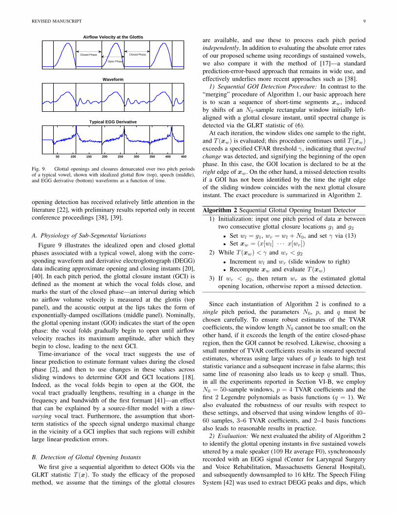
Fig. 9. Glottal openings and closures demarcated over two pitch periodsof a typical vowel, shown with idealized glottal flow (top), speech (middle),and EGG derivative (bottom) waveforms as a function of time.

opening detection has received relatively little attention in theliterature [22], with preliminary results reported only in recentconference proceedings [38], [39].

A. Physiology of Sub-Segmental Variations

Figure 9 illustrates the idealized open and closed glottalphases associated with a typical vowel, along with the corre-sponding waveform and derivative electroglottograph (DEGG)data indicating approximate opening and closing instants [20],[40]. In each pitch period, the glottal closure instant (GCI) isdefined as the moment at which the vocal folds close, andmarks the start of the closed phase—an interval during whichno airflow volume velocity is measured at the glottis (toppanel), and the acoustic output at the lips takes the form ofexponentially-damped oscillations (middle panel). Nominally,the glottal opening instant (GOI) indicates the start of the openphase: the vocal folds gradually begin to open until airflowvelocity reaches its maximum amplitude, after which theybegin to close, leading to the next GCI.

Time-invariance of the vocal tract suggests the use oflinear prediction to estimate formant values during the closedphase [2], and then to use changes in these values acrosssliding windows to determine GOI and GCI locations [18].Indeed, as the vocal folds begin to open at the GOI, thevocal tract gradually lengthens, resulting in a change in thefrequency and bandwidth of the first formant [41]—an effectthat can be explained by a source-filter model with a time-varying vocal tract. Furthermore, the assumption that short-term statistics of the speech signal undergo maximal changein the vicinity of a GCI implies that such regions will exhibitlarge linear-prediction errors.

B. Detection of Glottal Opening Instants

We first give a sequential algorithm to detect GOIs via theGLRT statistic T (x). To study the efficacy of the proposedmethod, we assume that the timings of the glottal closures

are available, and use these to process each pitch periodindependently. In addition to evaluating the absolute error ratesof our proposed scheme using recordings of sustained vowels,we also compare it with the method of [17]—a standardprediction-error-based approach that remains in wide use, andeffectively underlies more recent approaches such as [38].

1) Sequential GOI Detection Procedure: In contrast to the“merging” procedure of Algorithm 1, our basic approach hereis to scan a sequence of short-time segments xw, inducedby shifts of an N0-sample rectangular window initially left-aligned with a glottal closure instant, until spectral change isdetected via the GLRT statistic of (6).

At each iteration, the window slides one sample to the right,and T (xw) is evaluated; this procedure continues until T (xw)exceeds a specified CFAR threshold γ, indicating that spectralchange was detected, and signifying the beginning of the openphase. In this case, the GOI location is declared to be at theright edge of xw. On the other hand, a missed detection resultsif a GOI has not been identified by the time the right edgeof the sliding window coincides with the next glottal closureinstant. The exact procedure is summarized in Algorithm 2.

Algorithm 2 Sequential Glottal Opening Instant Detector1) Initialization: input one pitch period of data x between

two consecutive glottal closure locations g1 and g2• Set wl = g1, wr = wl +N0, and set γ via (13)• Set xw = (x[wl] · · · x[wr])

2) While T (xw) < γ and wr < g2

• Increment wl and wr (slide window to right)• Recompute xw and evaluate T (xw)

3) If wr < g2, then return wr as the estimated glottalopening location, otherwise report a missed detection.

Since each instantiation of Algorithm 2 is confined to asingle pitch period, the parameters N0, p, and q must bechosen carefully. To ensure robust estimates of the TVARcoefficients, the window length N0 cannot be too small; on theother hand, if it exceeds the length of the entire closed-phaseregion, then the GOI cannot be resolved. Likewise, choosing asmall number of TVAR coefficients results in smeared spectralestimates, whereas using large values of p leads to high teststatistic variance and a subsequent increase in false alarms; thissame line of reasoning also leads us to keep q small. Thus,in all the experiments reported in Section VI-B, we employN0 = 50-sample windows, p = 4 TVAR coefficients and thefirst 2 Legendre polynomials as basis functions (q = 1). Wealso evaluated the robustness of our results with respect tothese settings, and observed that using window lengths of 40–60 samples, 3–6 TVAR coefficients, and 2–4 basis functionsalso leads to reasonable results in practice.

2) Evaluation: We next evaluated the ability of Algorithm 2to identify the glottal opening instants in five sustained vowelsuttered by a male speaker (109 Hz average F0), synchronouslyrecorded with an EGG signal (Center for Laryngeal Surgeryand Voice Rehabilitation, Massachusetts General Hospital),and subsequently downsampled to 16 kHz. The Speech FilingSystem [42] was used to extract DEGG peaks and dips, which

REVISED MANUSCRIPT 10

100 200 300 400−1

−0.5

0

0.5

1Speech Waveform

x[n]

221 241 261 281 301−4

−2

0

2

4AR Coefficient Trajectories

a[n]

100 200 300 400−0.05

0

0.05

0.1

0.15EGG Derivative

DE

GG

[n]

221 241 261 281 3010

5

10

15

20GLRT Test Statistic

Sample Number

T(x

)

15% CFAR

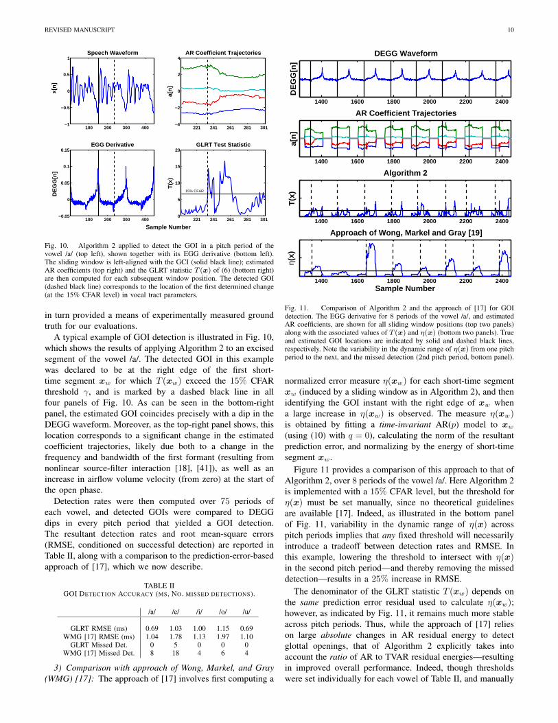
Fig. 10. Algorithm 2 applied to detect the GOI in a pitch period of thevowel /a/ (top left), shown together with its EGG derivative (bottom left).The sliding window is left-aligned with the GCI (solid black line); estimatedAR coefficients (top right) and the GLRT statistic T (x) of (6) (bottom right)are then computed for each subsequent window position. The detected GOI(dashed black line) corresponds to the location of the first determined change(at the 15% CFAR level) in vocal tract parameters.

in turn provided a means of experimentally measured groundtruth for our evaluations.

A typical example of GOI detection is illustrated in Fig. 10,which shows the results of applying Algorithm 2 to an excisedsegment of the vowel /a/. The detected GOI in this examplewas declared to be at the right edge of the first short-time segment xw for which T (xw) exceed the 15% CFARthreshold γ, and is marked by a dashed black line in allfour panels of Fig. 10. As can be seen in the bottom-rightpanel, the estimated GOI coincides precisely with a dip in theDEGG waveform. Moreover, as the top-right panel shows, thislocation corresponds to a significant change in the estimatedcoefficient trajectories, likely due both to a change in thefrequency and bandwidth of the first formant (resulting fromnonlinear source-filter interaction [18], [41]), as well as anincrease in airflow volume velocity (from zero) at the start ofthe open phase.

Detection rates were then computed over 75 periods ofeach vowel, and detected GOIs were compared to DEGGdips in every pitch period that yielded a GOI detection.The resultant detection rates and root mean-square errors(RMSE, conditioned on successful detection) are reported inTable II, along with a comparison to the prediction-error-basedapproach of [17], which we now describe.

TABLE IIGOI DETECTION ACCURACY (MS, NO. MISSED DETECTIONS).

/a/ /e/ /i/ /o/ /u/

GLRT RMSE (ms) 0.69 1.03 1.00 1.15 0.69WMG [17] RMSE (ms) 1.04 1.78 1.13 1.97 1.10

GLRT Missed Det. 0 5 0 0 0WMG [17] Missed Det. 8 18 4 6 4

3) Comparison with approach of Wong, Markel, and Gray(WMG) [17]: The approach of [17] involves first computing a

1400 1600 1800 2000 2200 2400

DEGG Waveform

DE

GG

[n]

1400 1600 1800 2000 2200 2400

AR Coefficient Trajectories

a[n

]

1400 1600 1800 2000 2200 2400

Algorithm 2

T(x

)1400 1600 1800 2000 2200 2400

Approach of Wong, Markel and Gray [19]

Sample Numberη(

x)

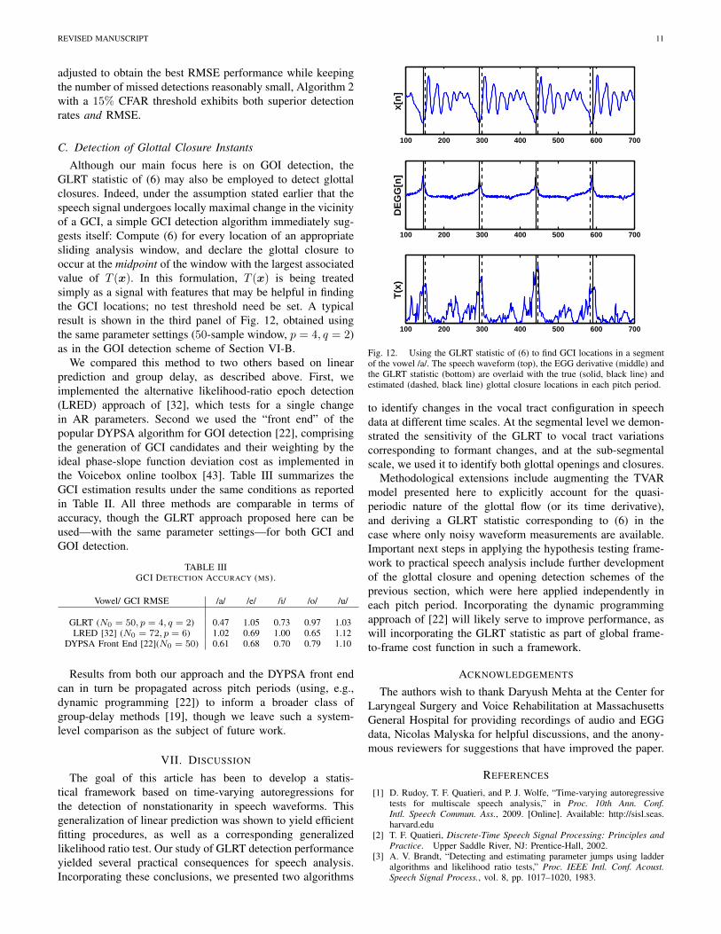
Fig. 11. Comparison of Algorithm 2 and the approach of [17] for GOIdetection. The EGG derivative for 8 periods of the vowel /a/, and estimatedAR coefficients, are shown for all sliding window positions (top two panels)along with the associated values of T (x) and η(x) (bottom two panels). Trueand estimated GOI locations are indicated by solid and dashed black lines,respectively. Note the variability in the dynamic range of η(x) from one pitchperiod to the next, and the missed detection (2nd pitch period, bottom panel).

normalized error measure η(xw) for each short-time segmentxw (induced by a sliding window as in Algorithm 2), and thenidentifying the GOI instant with the right edge of xw whena large increase in η(xw) is observed. The measure η(xw)is obtained by fitting a time-invariant AR(p) model to xw(using (10) with q = 0), calculating the norm of the resultantprediction error, and normalizing by the energy of short-timesegment xw.

Figure 11 provides a comparison of this approach to that ofAlgorithm 2, over 8 periods of the vowel /a/. Here Algorithm 2is implemented with a 15% CFAR level, but the threshold forη(x) must be set manually, since no theoretical guidelinesare available [17]. Indeed, as illustrated in the bottom panelof Fig. 11, variability in the dynamic range of η(x) acrosspitch periods implies that any fixed threshold will necessarilyintroduce a tradeoff between detection rates and RMSE. Inthis example, lowering the threshold to intersect with η(x)in the second pitch period—and thereby removing the misseddetection—results in a 25% increase in RMSE.

The denominator of the GLRT statistic T (xw) depends onthe same prediction error residual used to calculate η(xw);however, as indicated by Fig. 11, it remains much more stableacross pitch periods. Thus, while the approach of [17] relieson large absolute changes in AR residual energy to detectglottal openings, that of Algorithm 2 explicitly takes intoaccount the ratio of AR to TVAR residual energies—resultingin improved overall performance. Indeed, though thresholdswere set individually for each vowel of Table II, and manually

REVISED MANUSCRIPT 11

adjusted to obtain the best RMSE performance while keepingthe number of missed detections reasonably small, Algorithm 2with a 15% CFAR threshold exhibits both superior detectionrates and RMSE.

C. Detection of Glottal Closure Instants

Although our main focus here is on GOI detection, theGLRT statistic of (6) may also be employed to detect glottalclosures. Indeed, under the assumption stated earlier that thespeech signal undergoes locally maximal change in the vicinityof a GCI, a simple GCI detection algorithm immediately sug-gests itself: Compute (6) for every location of an appropriatesliding analysis window, and declare the glottal closure tooccur at the midpoint of the window with the largest associatedvalue of T (x). In this formulation, T (x) is being treatedsimply as a signal with features that may be helpful in findingthe GCI locations; no test threshold need be set. A typicalresult is shown in the third panel of Fig. 12, obtained usingthe same parameter settings (50-sample window, p = 4, q = 2)as in the GOI detection scheme of Section VI-B.

We compared this method to two others based on linearprediction and group delay, as described above. First, weimplemented the alternative likelihood-ratio epoch detection(LRED) approach of [32], which tests for a single changein AR parameters. Second we used the “front end” of thepopular DYPSA algorithm for GOI detection [22], comprisingthe generation of GCI candidates and their weighting by theideal phase-slope function deviation cost as implemented inthe Voicebox online toolbox [43]. Table III summarizes theGCI estimation results under the same conditions as reportedin Table II. All three methods are comparable in terms ofaccuracy, though the GLRT approach proposed here can beused—with the same parameter settings—for both GCI andGOI detection.

TABLE IIIGCI DETECTION ACCURACY (MS).

Vowel/ GCI RMSE /a/ /e/ /i/ /o/ /u/

GLRT (N0 = 50, p = 4, q = 2) 0.47 1.05 0.73 0.97 1.03LRED [32] (N0 = 72, p = 6) 1.02 0.69 1.00 0.65 1.12

DYPSA Front End [22](N0 = 50) 0.61 0.68 0.70 0.79 1.10

Results from both our approach and the DYPSA front endcan in turn be propagated across pitch periods (using, e.g.,dynamic programming [22]) to inform a broader class ofgroup-delay methods [19], though we leave such a system-level comparison as the subject of future work.

VII. DISCUSSION

The goal of this article has been to develop a statis-tical framework based on time-varying autoregressions forthe detection of nonstationarity in speech waveforms. Thisgeneralization of linear prediction was shown to yield efficientfitting procedures, as well as a corresponding generalizedlikelihood ratio test. Our study of GLRT detection performanceyielded several practical consequences for speech analysis.Incorporating these conclusions, we presented two algorithms

100 200 300 400 500 600 700

x[n

]

100 200 300 400 500 600 700

DE

GG

[n]

100 200 300 400 500 600 700

T(x

)

Fig. 12. Using the GLRT statistic of (6) to find GCI locations in a segmentof the vowel /a/. The speech waveform (top), the EGG derivative (middle) andthe GLRT statistic (bottom) are overlaid with the true (solid, black line) andestimated (dashed, black line) glottal closure locations in each pitch period.

to identify changes in the vocal tract configuration in speechdata at different time scales. At the segmental level we demon-strated the sensitivity of the GLRT to vocal tract variationscorresponding to formant changes, and at the sub-segmentalscale, we used it to identify both glottal openings and closures.

Methodological extensions include augmenting the TVARmodel presented here to explicitly account for the quasi-periodic nature of the glottal flow (or its time derivative),and deriving a GLRT statistic corresponding to (6) in thecase where only noisy waveform measurements are available.Important next steps in applying the hypothesis testing frame-work to practical speech analysis include further developmentof the glottal closure and opening detection schemes of theprevious section, which were here applied independently ineach pitch period. Incorporating the dynamic programmingapproach of [22] will likely serve to improve performance, aswill incorporating the GLRT statistic as part of global frame-to-frame cost function in such a framework.

ACKNOWLEDGEMENTS

The authors wish to thank Daryush Mehta at the Center forLaryngeal Surgery and Voice Rehabilitation at MassachusettsGeneral Hospital for providing recordings of audio and EGGdata, Nicolas Malyska for helpful discussions, and the anony-mous reviewers for suggestions that have improved the paper.

REFERENCES

[1] D. Rudoy, T. F. Quatieri, and P. J. Wolfe, “Time-varying autoregressivetests for multiscale speech analysis,” in Proc. 10th Ann. Conf.Intl. Speech Commun. Ass., 2009. [Online]. Available: http://sisl.seas.harvard.edu

[2] T. F. Quatieri, Discrete-Time Speech Signal Processing: Principles andPractice. Upper Saddle River, NJ: Prentice-Hall, 2002.

[3] A. V. Brandt, “Detecting and estimating parameter jumps using ladderalgorithms and likelihood ratio tests,” Proc. IEEE Intl. Conf. Acoust.Speech Signal Process., vol. 8, pp. 1017–1020, 1983.

REVISED MANUSCRIPT 12

[4] R. Andre-Obrecht, “A new statistical approach for the automatic seg-mentation of continuous speech signals,” IEEE Trans. Acoust. SpeechSignal Process., vol. 36, pp. 29–40, 1988.

[5] M. G. Hall, A. V. Oppenheim, and A. S. Willsky, “Time-varyingparametric modeling of speech,” Signal Process., vol. 5, pp. 267–285,1983.

[6] Y. Grenier, “Time-dependent ARMA modeling of nonstationary signals,”IEEE Trans. Acoust. Speech Signal Process., vol. 31, pp. 899–911, 1983.

[7] K. S. Nathan and H. F. Silverman, “Time-varying feature selection andclassification of unvoiced stop consonants,” IEEE Trans. Speech AudioProcess., vol. 2, pp. 395–405, 1994.

[8] K. Schnell and A. Lacroix, “Time-varying linear prediction for speechanalysis and synthesis,” in Proc. IEEE Intl. Conf. Acoust. Speech SignalProcess., 2008, pp. 3941–3944.

[9] S. M. Kay, “A new nonstationarity detector,” IEEE Trans. SignalProcess., vol. 56, pp. 1440–1451, 2008.

[10] S. Kay, Fundamentals of Statistical Signal Processing: Detection The-ory. Upper Saddle River, NJ: Prentice-Hall, 1998.

[11] D. Rudoy, P. Basu, T. F. Quatieri, B. Dunn, and P. J. Wolfe, “Adaptiveshort-time analysis-synthesis for speech enhancement,” in Proc. IEEEIntl. Conf. Acoust. Speech Signal Process., 2008, pp. 4905–4908.[Online]. Available: http://sisl.seas.harvard.edu

[12] D. Rudoy, P. Basu, and P. J. Wolfe, “Superposition frames for adaptivetime-frequency representations and fast reconstruction,” IEEE Trans.Signal Process., vol. 58, pp. 2581–2596, 2010.

[13] J. Vermaak, C. Andrieu, A. Doucet, and S. J. Godsill, “Particle methodsfor Bayesian modeling and enhancement of speech signals,” IEEE Trans.Speech Audio Process., vol. 10, pp. 173–185, 2002.

[14] R. C. Hendriks, R. Heusdens, and J. Jensen, “Adaptive time segmentationfor improved speech enhancement,” IEEE Trans. Audio Speech Lang.Process., vol. 14, pp. 2064–2074, 2006.

[15] V. Tyagi, H. Bourlard, and C. Wellekens, “On variable-scale piecewisestationary spectral analysis of signals for ASR,” Speech Commun.,vol. 48, pp. 1182–1191, 2006.

[16] G. S. Morrison, “Likelihood-ratio forensic voice comparison usingparametric representations of the formant trajectories of diphthongs,”J. Acoust. Soc. Am., vol. 125, pp. 2387–2397, 2009.

[17] D. Y. Wong, J. D. Markel, and A. H. Gray, “Least squares glottal inversefiltering from the acoustic speech waveform,” IEEE Trans. Acoust.Speech Signal Process., vol. 27, pp. 350–355, 1979.

[18] M. D. Plumpe, T. F. Quatieri, and D. A. Reynolds, “Modeling of theglottal flow derivative waveform with application to speaker identifica-tion,” IEEE Trans. Speech Audio Process., vol. 7, pp. 569–586, 1999.

[19] M. Brookes, P. A. Naylor, and J. Gudnasson, “A quantitative assessmentof group delay methods of identifying glottal closures in voiced speech,”IEEE Trans. Audio Speech Lang. Process., vol. 8, pp. 1017–1020, 2006.

[20] D. G. Childers and J. N. Larar, “Electroglottography for laryngealfunction assessment and speech analysis,” IEEE Trans. on Biomed. Eng.,vol. 31, pp. 807–817, 1984.

[21] J. S. Garofolo, L. Lamel, W. Fisher, J. Fiscus, D. Pallett, N. Dahlgren,and V. Zue, TIMIT Acoustic-Phonetic Continuous Speech Corpus.Philadelphia, PA: Linguistic Data Consortium, 1993.

[22] P. A. Naylor, A. Kounoudes, J. Gudnasson, and M. Brookes, “Estimationof glottal closure instants in voiced speech using the DYPSA algorithm,”IEEE Trans. Audio Speech Lang. Process., vol. 15, pp. 34–43, 2007.

[23] L. A. Liporace, “Linear estimation of non-stationary signals,” J. Acoust.Soc. Am., vol. 58, pp. 1268–1295, 1975.

[24] M. K. Tsatsanis and G. B. Giannakis, “Time-varying system identifica-tion and model validation using wavelets,” IEEE Trans. Signal Process.,vol. 41, pp. 3512–3523, 1993.

[25] T. S. Rao, “The fitting of non-stationary time series models with timedependent parameters,” J. Roy. Stat. Soc. B, vol. 32, pp. 312–322, 1970.

[26] G. Kitagawa and W. Gersch, “A smoothness priors time-varying ARcoefficient modeling of nonstationary covariance time series,” IEEETrans. Automat. Control, vol. 30, pp. 48–56, 1985.

[27] T. Hsiao, “Identification of time-varying autoregressive systems usingmaximum a posteriori estimation,” IEEE Trans. Signal Process., vol. 56,pp. 3497–3509, 2008.

[28] S. Kay, Modern Spectral Estimation: Theory and Application. UpperSaddle River, NJ: Prentice-Hall, 1988.

[29] M. Kendall, A. Stuart, J. K. Ord, and S. Arnold, Kendall’s AdvancedTheory of Statistics. Hodder Arnold, 1999, vol. 2a.

[30] J. W. Brewer, “Kronecker products and matrix calculus in systemtheory,” IEEE Trans. Circuits Syst., vol. 25, pp. 772–781, 1978.

[31] S. D. Gupta and M. D. Perlman, “Power of the noncentral F-test: Effectof additional variates on Hotelling’s t2 test,” J. Am. Statist. Ass., vol. 69,pp. 174–180, 1974.

[32] E. Moulines and R. D. Francesco, “Detection of the glottal closureby jumps in the statistical properties of the speech signal,” SpeechCommun., vol. 9, pp. 401–418, 1990.

[33] J. P. Bello, L. Daudet, S. Abdallah, C. Duxbury, and M. Davies, “Atutorial on onset detection in music signals,” IEEE Trans. Speech AudioProcess., vol. 13, pp. 1035–1048, 2005.

[34] S. Jarifia, D. Pastora, and O. Rosec, “A fusion approach for automaticspeech segmentation of large corpora with application ot speech synthe-sis,” Speech Communication, vol. 50, pp. 67–80, 2008.

[35] R. E. Quandt, “Tests of the hypothesis that a linear regression systemobeys two separate regimes,” J Amer. Stat. Assoc., vol. 55, pp. 324–330,1960.

[36] S. L. Marple, Digital Spectral Analysis. Englewood Cliffs, NJ: Prentice-Hall, 1987.

[37] K. Sjolander and J. Beskow. (2005) WaveSurfer 1.8.5 for Windows.KTH Royal Institute of Technology. [Online]. Available: http://www.speech.kth.se/wavesurfer/wavesurfer-185-win.zip

[38] T. Drugman and T. Dutoit, “Glottal closure and opening instant detectionfrom speech signals,” in Proc. 10th Ann. Conf. Intl. Speech Commun.Ass., 2009.

[39] M. P. Thomas, J. Gudnason, and P. A. Naylor, “Detection of glottalclosing and opening instants using an improved DYPSA framework,” inProc. 17th Eur. Signal Process. Conf, Glasgow, Scotland, 2009.

[40] N. Henrich, C. d’Alessandro, B. Doval, and M. Castellengo, “On theuse of the derivative of electroglottographic signals for characterizationof nonpathological phonation,” J. Acoust. Soc. Am., vol. 115, pp. 1321–1332, 2004.

[41] T. V. Ananthapadmanabha and G. Fant, “Calculation of true glottal flowand its components,” Speech Commun., vol. 1, pp. 167–184, 1982.

[42] M. Huckvale. (2000) Speech filing system: Tools for speechresearch. University College London. [Online]. Available: http://www.phon.ucl.ac.uk/resource/sfs

[43] M. Brookes. (2006) VOICEBOX: A speech processing toolboxfor MATLAB. Imperial College London. [Online]. Available: http://www.ee.imperial.ac.uk/hp/staff/dmb/voicebox/voicebox.html