Embed Size (px)
Citation preview

EI @ Haas WP 235R
A Ban on One is a Boon for the Other: Strict Gasoline Content Rules and Implicit Ethanol Blending
Mandates
Soren Anderson and Andrew Elzinga December 2012
Revised version published in the Journal of Environmental Economics and Management,
67 (3): 258 – 273 (May 2014)
Energy Institute at Haas working papers are circulated for discussion and comment purposes. They have not been peer-reviewed or been subject to review by any editorial board. © 2013 by Soren Anderson and Andrew Elzinga. All rights reserved. Short sections of text, not to exceed two paragraphs, may be quoted without explicit permission provided that full credit is given to the source.
http://ei.haas.berkeley.edu

A Ban on One Is a Boon for the Other: Strict GasolineContent Rules and Implicit Ethanol Blending Mandates∗
Soren Anderson†
Michigan State UniversityNBER
Andrew Elzinga‡
Brown University
December 19, 2012
Abstract
Ethanol and methyl-tertiary butyl ether (MTBE) were close substitutes in the gasolineadditives market until MTBE was banned due to concerns about groundwater contami-nation, leading to a sudden and dramatic substitution toward ethanol as an alternativeoxygenate and octane-booster. We use variation in the timing of MTBE bans across statesto identify their effects on gasoline prices. We find that state bans increased reformulatedgasoline prices by 6 cents in non-Midwestern states for which the bans were binding, withlarger impacts during times of high ethanol prices relative to MTBE and crude oil. We findqualitatively similar, yet smaller effects for conventional gasoline. We argue on the basis ofa simple conceptual model and supporting empirical evidence that these bans functioned asimplicit state-level ethanol blending mandates in areas that were previously using MTBE tocomply with strict environmental constraints. Overall, our results are consistent with thetheoretical prediction that mandating a minimum market share for a more costly alternativefuel—either directly, or implicitly through a ban on the preferred conventional fuel—willinevitably increase fuel prices in a competitive market.
JEL classification numbers: Q4Key words: ethanol; gasoline; MTBE; gasoline content regulations
∗We are grateful to Malika Chaudhuri and Chris Peterson for their help in obtaining MTBE price data,Don Fullerton and Lucas Davis for helpful comments, and seminar participants at the NTA Meetings inNovember 2010. This research was supported in part under a research contract from the California EnergyCommission to the Energy Institute at Haas.†Email: [email protected]. Web address: http://www.msu.edu/∼sta.‡Email: andrew [email protected].

1 Introduction
Gasoline refiners have faced a series of increasingly stringent environmental constraints in
recent decades, which have significantly narrowed their options for maintaining high levels of
fuel octane.1 By the late 1990s, suppliers in many cities came to rely heavily on a chemical
fuel additive known as MTBE (methyl-tertiary butyl ether) to boost octane in the presence
of environmental constraints, while suppliers in a handful of other cities used ethanol instead.
Like ethanol, MTBE was valued for its energy content, high oxygen content, high octane
rating, and clean-burning properties—but was found to leak from underground storage tanks,
contaminating groundwater supplies. Thus, a total of 19 states banned MTBE in gasoline
from 2000–2006 before it was phased out nationwide in mid-2006, leading to a sudden and
dramatic substitution toward ethanol as an alternative oxygenate and octane booster. We
use a combination of applied theory, econometric estimation, and institutional background
to shed light on this era of gasoline content regulation, which came after a flurry of regulatory
activity flowing out of the Clean Air Act Amendments in the early 1990s, and which served
as prelude to the implementation of the federal Renewable Fuel Standard in the late 2000s.
We show theoretically that MTBE bans function as implicit ethanol blending mandates in
the presence of strict environmental constraints that compel refiners to blend either MTBE
or ethanol. We confirm this interpretation empirically by examining ethanol and MTBE
blend shares before and after the enforcement of state MTBE bans, finding that they had
large, discrete, and immediate effects on ethanol blending shares, consistent with direct
substitution. We then use variation in the timing of MTBE bans across states to identify
their effects on gasoline prices. We distinguish the heterogeneous effects of these bans by
(1) conventional gasoline versus reformulated gasoline, which faced more stringent environ-
mental constraints that led to highly inelastic demand for ethanol as a substitute blending
1High-octane fuels are more resistant to “knocking,” which occurs when the pressurized fuel-air mixturein the engine ignites prior to the spark plug firing, reducing engine efficiency. Thus, octane is a criticalmeasure of gasoline quality, and the need for high-octane fuel has risen over time with improvements inengine performance.
1

component, (2) geography, to account for whether the bans were binding or not, and (3)
time, based on shifts in the wholesale prices for ethanol, MTBE, and crude oil—the key
commodity inputs into oxygenate-blended gasoline.
We find that state MTBE bans increased reformulated gasoline prices by 6 cents in
non-Midwestern states, for which the bans were binding, with little effect in the Midwest,
which was already using ethanol. In contrast, we find minimal effect on average prices
for conventional gasoline, which faced less stringent blending requirements, regardless of
location. As expected, price impacts were larger when ethanol prices were high relative
to MTBE and crude oil, and again, these effects were more pronounced for reformulated
gasoline than for conventional gasoline. In addition, we find that MTBE bans increased
the monthly pass-through rate of wholesale ethanol prices into retail gasoline prices, while
decreasing the pass-through rates of wholesale MTBE and crude oil prices. Importantly,
we find that state MTBE bans that took effect after the unexpected nationwide ban have
virtually no effect on gasoline prices, which eases potential concerns about differential price
trends in states with MTBE bans. Overall, our results are consistent with the theoretical
prediction that a ban on a less costly conventional fuel, which in extreme cases operates as
a de-facto mandate for the more costly alternative fuel, will inevitably increase fuel prices
in a competitive market.
This paper is closely related to a recent empirical literature that exploits variation in gaso-
line content regulations across locations and over time to identify their effects on gasoline
prices, mainly using reduced-form empirical methods. In general, this literature finds that
gasoline content regulations increase average prices (Muehlegger 2006; Chouinard and Perloff
2007; Brown, Hastings, Mansur and Villas-Boas 2008; Chakravorty, Nauges and Thomas
2008), while seasonally and geographically differentiated regulations segment markets in
ways that limit arbitrage over time and across space, exacerbating local price spikes follow-
ing refinery outages (Muehlegger 2006; Brown et al. 2008) and increasing opportunities for
refiners to exercise market power (Brown et al. 2008; Chakravorty et al. 2008). Overall, how-
2

ever, environmental regulations explain a relatively small fraction of the variation in gasoline
prices, which is largely driven by crude oil and state, local, and federal taxes (Chouinard
and Perloff 2007).2
Our paper contributes to this literature in three ways. First, while previous papers focus
on the gasoline content regulations flowing directly from the Clean Air Act Amendments of
the early 1990s, we focus on state MTBE bans, which occurred later, which apply to gasoline
sold everywhere in a state, and which likely had different impacts on prices. Thus, our paper
helps document an important era in gasoline content regulation that led to a significant
increase in ethanol consumption, well before the implementation of the federal Renewable
Fuel Standard (RFS) in the late 2000s. In particular, these bans are important pre-existing
regulations that must be considered when assessing the marginal impacts of the federal RFS
on gasoline markets.
Second, like previous studies, we allow gasoline content regulations to have heterogeneous
effects on gasoline prices according to location and the level of regulatory stringency. In
particular, we allow the effects of MTBE bans to differ for Midwestern states, which were
closer to ethanol supply, as well as for conventional gasoline, which faced much less stringent
environmental regulations. Unlike previous studies, however, we allow the effects of gasoline
content regulations to vary over time according to the prices of key gasoline inputs, since
2Brown et al. (2008) estimate the effects of federal Reid Vapor Pressure (RVP) and reformulated gasoline(RFG) regulations on weekly wholesale prices in affected cities, controlling for wholesale prices in nearbycities that lacked such regulations. They find prices in treated cities increased following the onset of theregulations, while the number of wholesalers decreased, suggesting that market power played a role inthe price increase. They also find that gasoline price volatility increased in treated cities, arguing thatgeographically fragmented regulations limit opportunities to arbitrage prices across locations. Chakravortyet al. (2008) use a state-panel design to estimate the effect of reformulated gasoline and winter oxygenatedfuel regulations (measured by the fraction of a state’s population subject to such regulations) on state-averageannual gasoline prices, also finding that such regulations led to higher fuel prices, both by increasing refiningand distribution costs and by segmenting gasoline markets in a way that increased market power of refineries.Muehlegger (2006) estimates the impact of gasoline content regulations on prices using a structural modelof refinery behavior, which he estimates using data on monthly average prices and quantities by state. Hefinds that content regulations led to higher average prices through higher refining and distribution costsand that geographically uniform regulations could substantially mitigate the severity of local price spikes.Finally, Chouinard and Perloff (2007) use a state-panel design to estimate the effects of crude oil prices,taxes, refiner market power, vertical integration, and environmental regulations on gasoline prices, findingthat environmental regulations explain a relatively small fraction of the overall costs.
3

the bans dramatically shift the demand for these inputs. Thus, our estimates may have
greater external validity in the face of changing market conditions. Importantly, modeling
heterogeneity based on input prices also addresses potential concerns about spillovers of state-
level policies to gasoline prices in other states via national wholesale markets for gasoline
and fuel additives—something that is ignored in previous studies.
Third, we argue on the basis of a simple conceptual model and supporting empirical
evidence that state MTBE bans approximated direct state-level ethanol blending mandates
in areas that were previously using MTBE to comply with strict oxygenation requirements
or to maintain fuel octane levels in the presence of other environmental constraints. Theory
implies that a fractional ethanol blending mandate acts like a tax on gasoline and a subsidy
for ethanol, increasing average fuel prices when the ethanol supply curve is more steeply
sloped than that of gasoline, and calibrated simulation models bear this prediction out
(Holland, Knittel and Hughes 2008). Yet controversy regarding the effects of ethanol blending
mandates on gasoline prices continues to fester, due in large part, we suspect, to the conflation
of higher ethanol production in general with specific ethanol policies that lead to higher
production—along with the difficulty of distinguishing statistically the effects of the national
mandate from other trends affecting gasoline prices (see Knittel and Smith 2012). Thus, our
results are relevant not just for understanding the impacts of the MTBE bans during this era,
but also for inferring the potential impacts of ethanol mandates on gasoline prices, thereby
helping to inform an important current policy debate. In this case, our results suggest that
direct, state-level ethanol blending mandates would have increased fuel prices. Our approach
may prove useful in other contexts, when the reduced-form impact of a new or future policy
cannot be estimated, but can be inferred from a surrogate policy sharing a similar economic
structure.3
3Other policies that share a similar economic structure include the U.S. federal Renewable Fuel Standard(RFS) and California’s Low-Carbon Fuel Standard (LCFS). While the federal RFS is legislated as a minimumquantity, it is implemented by EPA as a minimum market share requirement. Likewise, in the case of aconventional high-carbon fuel (gasoline) and a single low-carbon fuel (say ethanol), the LCFS is equivalentto a minimum market share for the low-carbon fuel.
4

In addition, our paper contributes to a more general applied theory and empirical eco-
nomic literature on overlapping environmental policies and rent-seeking behavior in environ-
mental regulation. Gasoline refiners now face a host of overlapping constraints on gasoline
content. Our paper illustrates how a ban on a gasoline input (MTBE) can—in the presence of
other environmental policy constraints—lead to dramatic substitution toward one particular
close substitute (ethanol). In the extreme, when other options have been eliminated through
regulation, a ban on one input operates as a de-facto mandate for its alternative. Exces-
sive regulation also comes with a hidden political cost: eliminating substitute technologies
through regulation inflates incentives for rent-seeking behavior among the industries whose
technologies remain viable. Indeed, ethanol producers were among the most ardent sup-
porters of MTBE bans, with virtually all corn-growing Midwestern states banning MTBE,
despite the fact that few of these states had problems with MTBE contamination.
The rest of this paper proceeds is as follows. Section 2 discusses important background
on the economics of ethanol and MTBE blending in the United States before presenting our
conceptual model. Section 3 presents descriptive evidence on MTBE bans and their effects
on ethanol usage. Section 4 describes our estimation strategy and presents our regression
results for the effects of MTBE bans on retail gasoline prices. Section 5 summarizes and
concludes.
2 Industry background and conceptual model
Historically, ethanol and MTBE have been used for several reasons, including to boost fuel
octane levels, to comply with minimum fuel oxygenation requirements, and to extend fuel
supplies during times of relatively high crude oil prices. In this section, we briefly review
the history of environmental regulation that led gasoline suppliers to blend either ethanol or
MTBE for these reasons, as well as the slate of bans that eliminated MTBE from gasoline
during the 2000s. We discuss the economics of ethanol versus MTBE blending, and we
5

outline a simple conceptual model that clarifies the predicted effects of MTBE bans—as well
as the conditions under which such bans approximate direct ethanol blending mandates.
Our goal is to motivate our empirical analyses below, which are based on comparing gasoline
markets across states before and after the MTBE bans took effect.
2.1 Maintaining octane under strict environmental constraints
A major theme in the gasoline refining industry over the past four decades has been the
industry’s struggle to maintain fuel octane levels in the face of increasingly stringent environ-
mental constraints. With each new environmental regulation, refiners have responded with
new, cost-minimizing approaches to maintain octane, leading to new, often unanticipated en-
vironmental side-effects, leading in turn to further environmental regulations. Over time, this
pattern of regulation, industry response, and further regulation has significantly narrowed
the set of octane-enhancing options available to refiners. Thus, by the late 1990s, suppliers
in many cities had few cost-effective alternatives outside of blending ethanol or MTBE. In
such contexts—that is, when gasoline suppliers are compelled to blend either ethanol or
MTBE to maintain octane or to comply with explicit fuel oxygenation requirements—bans
on MTBE act as de-facto ethanol mandates. This is the key insight of our paper.4
Initially, gasoline refiners blended an octane-rich, lead-based compound into gasoline,
but the widespread use of leaded gasoline was found to generate significant public health
and environmental impacts. Thus, the EPA began regulating leaded gasoline in the 1970s,
leading to its eventual ban in the 1980s. Industry responded by altering the refining process
to boost the production of high-octane aromatic hydrocarbons, such as benzene and toluene,
as well as butane, which is a high-octane byproduct of this altered refining process. However,
benzene was a suspected carcinogen, while the increased use of aromatics and butane led to
a significant rise in emissions of evaporative volatile organic compound (VOCs)—precursors
to the formation of ground-level ozone. Meanwhile, some cities were experiencing elevated
4The discussion of gasoline production and environmental regulation in this section relies heavily onStikkers (2002) and Brown et al. (2008).
6

levels of carbon monoxide emissions due to incomplete combustion of fuel during cold winter
months. Thus, in the 1990s, the EPA placed caps on Reid Vapor Pressure (RVP) in select
cities to limit evaporative emissions of VOCs, began requiring oxygenate blending in select
cities during winter months to reduce emissions of carbon monoxide, and required so-called
reformulated gasoline (RFG) in select cities with particularly poor air quality. These changes
were authorized by Congress in a series of amendments to the Clean Air Act. Fuel sold
under the RFG program was subject to a suite of environmental constraints, including caps
on Reid Vapor Pressure (RVP), caps on aromatic hydrocarbon content, and caps on benzene
and other toxic substances, as well as mandated year-round blending of oxygenates—almost
always provided by ethanol or MTBE.5,6,7
Thus, by the late 1990s, gasoline suppliers faced a multitude of restrictions on gasoline
content that generated strong incentives to blend either ethanol or MTBE into gasoline,
with the strength of these incentives varying geographically according to the stringency
of the local environmental regulations. At one extreme, producers selling gasoline under
the RFG program were required to blend either ethanol or MTBE into gasoline to comply
with explicit oxygenation mandates—and faced additional caps on aromatics and toxics that
likely would have led them to blend ethanol or MTBE regardless, simply to maintain octane
levels. In somewhat less extreme cases, producers selling conventional gasoline under the
winter oxygenation program were required to blend either ethanol or MTBE, but only during
5Limits on RVP were phased-in gradually during the early 1990s. A fuel’s RVP measures its propensity toevaporate and therefore generate emissions of VOCs, which react with nitrogen oxides (NOx) in the presenceof sunlight to form ground-level ozone, causing respiratory illness. Auffhammer and Kellogg (2011) showthat limits on RVP were ineffective outside of California, since refiners responded by reducing butane, whichis not particularly potent for smog formation. In contrast, California’s unique regulations targeted the mostpotent VOCs directly, leading to significant improvements in air quality.
6Winter oxygenation requirements took effect in 39 cities in the early 1990s, mandating a minimum of2.7% oxygen by weight in most areas, which translated to 7.4% ethanol or 15.0% MTBE by volume; mostremaining areas required 3.1% oxygen by weight. While oxygenates other than ethanol and MTBE wereavailable, virtually all demand was met with these two oxygenates. Oxygenates help gasoline burn morecompletely in older engines that lack carburetors, reducing carbon monoxide emissions. Most cities havesince exited the program due to improved air quality.
7The RFG program was mandated for nine large cities with the worst smog, and a number of other citiesopted to join the program voluntarily. The program began in 1995, superseding existing RVP and winteroxygenation programs in some cities. The program required 2.1% oxygen by weight in most areas, whichtranslated to 5.8% ethanol or 11.7% MTBE by volume.
7

winter months. Lastly, even producers selling conventional gasoline in locations without such
requirements sometimes opted to blend ethanol or MTBE to boost octane or to extend fuel
supplies when prices for these additives were sufficiently low. These myriad restrictions set
the stage for the MTBE bans that were to come and the resulting dramatic shift to ethanol.
By the late 1990s, some cities began to notice that MTBE, a suspected carcinogen, was
contaminating their drinking water. Because this problem was most pronounced in areas with
RFG, it soon became clear that the contamination was coming from leaking underground
gasoline storage tanks. Thus, starting around 2000, a number of states begin to ban MTBE
in gasoline, and pressure built for a nationwide ban.8 Meanwhile, the fuel industry sought
liability protection against lawsuits stemming from MTBE contamination, arguing that they
should not be penalized for blending MTBE when they were compelled to do so by federal
environmental regulation. Finally, in late 2005, the Energy Policy Act of 2005 failed to grant
the liability protection that MTBE blenders were seeking. Given the large number of state
MTBE bans and rising concerns about liability risk, the industry treated this failed legislative
remedy as an implicit ban on MTBE and opted to phase-out the use of the chemical almost
entirely by the summer of 2006. Given the myriad restrictions on gasoline content that were
already in place, these explicit and implicit MTBE bans acted as de-facto ethanol mandates
in RFG cities, as well as in cities subject to minimum oxygenation requirements during
winter months, and led to increased demand for ethanol in other areas and at other times
to boost octane or to extend fuel supplies.9
8Political economy motivations were also clearly at play. State and federal MTBE bans were stronglysupported by the Midwest-based ethanol industry. Indeed, most Midwestern states had MTBE bans, despitethe fact that relatively few Midwestern cities required RFG and that most Midwestern suppliers would havechosen ethanol over MTBE anyway, given ethanol’s proximity.
9Besides failing to grant liability protection for the use of MTBE, the 2005 legislation eliminated theexplicit oxygenation requirement in RFG, which made the threat of legal liability even more salient. Ratherthan cease oxygenate blending altogether, however, refiners switched to ethanol, as we show below, despitethe removal of the oxygenation requirement. Why? There are two probable reasons. First, given otherconstraints on aromatics and toxics, continuing to blend ethanol may in fact have been the cheapest wayto maintain fuel octane. Second, the same legislation that removed the oxygenation requirement for RFGalso imposed the federal Renewable Fuel Standard (RFS), which mandated a minimum quantity of ethanolblending in the overall fuel supply, equal to roughly 5% of gasoline consumption in 2012. Thus, makingcostly changes to the refining process in an effort to boost octane in other ways would have been unwise,given that the looming RFS would soon lead to increased octane anyway via mandated ethanol blending.
8

2.2 Ethanol versus MTBE blending economics
While ethanol and MTBE are close substitutes in the gasoline additives market, their produc-
tion, distribution, and integration into the gasoline supply chain differ in several important
ways. Unlike ethanol, MTBE is typically produced and mixed with gasoline directly at
petroleum refineries.10 After the blending is complete, the finished gasoline can be shipped
through refined product pipelines virtually anywhere in the country at low cost (Trench
2001). Alternatively, the MTBE itself can be shipped independently via pipeline to whole-
sale distribution terminals, blended immediately with an MTBE-ready gasoline blendstock,
and then stored as finished gasoline in common storage tanks.
Ethanol, by contrast, is produced in geographically isolated refineries in the Midwest,
far away from most petroleum refineries and large cities, and unlike MTBE, it cannot be
shipped through existing refined product pipelines.11 Instead, ethanol must be transported at
relatively high cost via rail, barge, or tanker truck to wholesale fuel blending and distribution
terminals. The cost of transporting ethanol by rail from the Midwest to the coasts, for
example, is about 15 cents per gallon (Hughes 2011). Upon arrival at the terminals, ethanol is
stored separately from gasoline in dedicated tanks and then, in the final step, splash blended
with an ethanol-ready gasoline blendstock in the tank of a delivery truck for transmission to
an individual retail outlet.
These differences between ethanol and MTBE supply and distribution have two key con-
sequences. First, high transportation costs, limited fungibility in refined product pipelines,
and (until recently) the lack of blending infrastructure outside of the Midwest seriously con-
10MTBE is a petroleum-based chemical fuel additive. It is produced by reacting methanol with isobutylenein dedicated MTBE production facilities or by using byproduct streams of isobutylene at petroleum refineriesor petrochemical ethylene plants (Lidderdale 2001).
11Existing pipelines are not suitable for two reasons. First, existing pipelines are configured to transporthigh volumes of gasoline from large oil refineries to cities, whereas ethanol refineries are smaller, located inrural agricultural areas, and are widely dispersed. Second, water tends to accumulate at low points in refinedproduct pipelines. Unlike petroleum, ethanol mixes with water, and so pure ethanol cannot be shipped viaexisting pipelines, lest it become contaminated. Likewise, if ethanol-blended gasoline comes into contactwith water, the ethanol will separate from the gasoline and combine with the water. Thus, ethanol must beshipped separately and only blended in the last step.
9

Figure 1: Fuel price trends
Huricane Katrina Nationwide Lehman BrothersBankruptcy
01
23
4W
hole
sale
pric
e, $
/gal
lon
1996m1 1998m1 2000m1 2002m1 2004m1 2006m1 2008m1 2010m1Date
Gasoline
MTBE Ban
Ethanol
MTBE
MTBE BanSeptember 11, 2001
Note: This figure shows monthly wholesale rack prices for gasoline (U.S. average),
MTBE (Gulf Coast), and ethanol (in Omaha, Nebraska). Ethanol prices are net
of the federal ethanol blending incentive. Prices are in real 2010 dollars. See text
for details.
strained opportunities for ethanol price arbitrage across locations in response to high prices
for gasoline or for competing oxygenates and octane enhancers. Thus, while MTBE prices
track gasoline prices very closely over time, ethanol prices do not. See Figure 1. Wholesale
MTBE prices track wholesale gasoline prices closely, rarely falling below the price of gaso-
line and sometimes spiking above it. This behavior is consistent with MTBE being a close
substitute for gasoline, except for in rare cases when MTBE supply falls short relative to
inelastic oxygenate demand.
Second, ethanol’s high transportation costs lead to significant geographic variation in
ethanol usage. Thus, prior to the bans, suppliers of RFG on the coasts, facing relatively
high ethanol transportation costs, tended to choose MTBE, while suppliers of RFG in the
Midwest, facing relatively low transportation costs, and in some cases encouraged by attrac-
10

tive ethanol blending subsidies, chose ethanol.
Other cost considerations were also relevant. First, ethanol has higher RVP than MTBE,
which in turn has higher RVP than gasoline. Thus, for suppliers subject to RVP constraints,
choosing ethanol would have required reducing the RVP of the underlying gasoline blend-
stock, which is costly. As a result, suppliers of RFG that chose ethanol rarely blended
the full 10% of ethanol allowed by EPA regulations, just the minimum needed to meet the
oxygenation mandate. Second, suppliers subject to winter oxygenation requirements also
tended to choose ethanol, regardless of location, due to ethanol’s higher oxygen content per
volume and the lack of RVP limits in such locations. Finally, ethanol blending was sup-
ported by a federal subsidy of roughly $0.50 per gallon during this time period, which only
recently expired. All told, ex-ante estimates were that the MTBE bans would increase RFG
prices by 3.6 cents per gallon on average, with larger increases in coastal states (U.S. Energy
Information Administration 2003).
2.3 Direct and indirect ethanol blending mandates
Figure 2(a) presents stylized model of a perfectly competitive state fuel market in the pres-
ence of a percent ethanol blending mandate. The demanders in this market are fuel blenders,
implicitly buying ethanol and gasoline on behalf of retail consumers. For simplicity, these
retail consumers are assumed to have perfectly inelastic overall demand for fuel, which is
given by the width of the horizontal axis, while treating ethanol and gasoline as perfect sub-
stitutes.12 Thus, fuel blenders inherit these preferences, as well, attempting to minimize the
overall cost of fuel, subject to their inelastic demand, while also meeting their fuel blending
12These assumptions are consistent with vast empirical evidence showing that overall demand for fuel isinelastic, perhaps declining to less than 0.1 in magnitude in recent years (Small and Dender 2007; Hughes,Knittel and Sperling 2008), as well as more recent empirical evidence showing that consumers in the UnitedStates and Brazil treat high-concentration ethanol blends and gasoline as very close, albeit not perfect,substitutes (Anderson 2012; Salvo and Huse 2012). Given our focus here on low-concentration ethanol blends,for which ethanol concentrations are rarely transparent to consumers, and for which impacts on driving rangeand performance are negligible, the assumption of perfect substitutes is an even better approximation. Inaddition, for simplicity, we abstract away from differences in energy content, which are minor when blendingsmall fractions of ethanol.
11
obligations. The suppliers in this market are fuel refiners and distributors that produce fuel
and deliver it to market. Gasoline supply is represented as a horizontal marginal cost curve,
while ethanol supply is represented as an upward-sloping marginal cost curve.13 Before the
ethanol mandate takes effect, blenders of ethanol are only willing to pay up to the marginal
cost of gasoline. Thus, ethanol’s market price and quantity are given by point A, at which
the marginal cost of ethanol equals the marginal cost of gasoline, with a small amount of
ethanol competing directly as a gasoline substitute.14 Thus, small shifts in gasoline supply
pass through fully to fuel prices, while small shifts in the ethanol supply pass through not
at all.
After the ethanol mandate takes effect, fuel blenders are forced to increase their ethanol
demand to point B, at which ethanol’s marginal cost exceeds that of gasoline. At the
standard, the marginal cost to blenders of acquiring one more gallon of fuel while remaining
in compliance with the standard—and therefore, the fuel price that retail consumers will
pay—is the quantity-weighted average of ethanol’s and gasoline’s marginal costs.15 Thus,
the impact of the mandate on fuel prices is higher when either ethanol supply shifts up or
when gasoline supply shifts down. Small shifts in gasoline supply now pass through only
partially to fuel prices, and similarly for ethanol supply, according to their respective shares
in the overall fuel supply, given by the ethanol mandate.
Figure 2(b) presents a similar figure for a competitive state fuel market in the presence
of inelastic demand for oxygenates (to satisfy a minimum oxygenation requirement or to
13An approximately horizontal state gasoline supply curve is consistent with a large national marketand low transportation costs via refined product pipelines. In contrast, an upward-sloping ethanol supplycurve is consistent with a smaller national market, geographic dispersion of ethanol refineries, relativelyhigh transportation costs, limited infrastructure for ethanol blending at terminals, and relatively few retailstorage tanks that can handle ethanol-blended fuel.
14We have drawn the initial equilibrium as an interior solution. In general, corner solutions at zero or at the10% upper limit for ethanol blending are also possible. In the former case, our conclusions are unchanged. Inthe latter case, the ethanol mandate is not binding. The so-called “blend wall” of 10% ethanol is determinedby EPA regulation (only recently increased to 15%) and by manufacturer warranties for most cars.
15While we have arbitrarily drawn in the ethanol standard at a 50% blend share, so that the marginal costof fuel is shown as the simple average of ethanol’s and gasoline’s marginal costs, this obviously need not bethe case. For example, at a 10% blend share, the marginal cost of fuel would be 10% of ethanol’s marginalcost plus 90% of gasoline’s marginal cost.
12

Figure 2: Illustration of conceptual model
P i ($/ ll ) Eth l
(a) Direct ethanol mandate
MCETHANOL
Price ($/gallon) Ethanol mandate
ETHANOL
B
MCFUEL (with mandate)P
B
MCPBEFORE
PAFTER
A MCGASOLINEA
Ethanol Gasoline
P i ($/ ll ) O t
(b) Indirect ethanol mandate (via MTBE ban)
MCETHANOL
Price ($/gallon) Oxygenate demand
ETHANOL
B
PMCFUEL (with MTBE ban)
B
PAFTER
A MCMTBE
MCPBEFORE
MCGASOLINE
Ethanol GasolineMTBE
Note: Figure (a) illustrates the effects of a direct percent ethanol blending man-
date. Figure (b) illustrates the effects of an MTBE ban in the presence of inelastic
percent oxygenate demand satisfied using ethanol and/or MTBE. The ethanol
mandate in (a) and the MTBE ban in (b) have virtually identical effects when
MTBE supply hugs gasoline supply. See text for details.
13

enhance octane) and potential ban on MTBE; the same qualitative results would hold with
more elastic oxygenate demand. Again, gasoline supply is horizontal, while ethanol supply
is upward-sloping. The supply of MTBE is represented as a horizontal supply curve at
or just above the marginal cost of gasoline.16 In the absence of a ban on MTBE, ethanol’s
marginal cost and quantity supplied are given by point A, at which a small amount of ethanol
competes with MTBE in the market for oxygenates. At this point, the marginal cost of fuel
is set by the quantity-weighted average of gasoline and oxygenates, the latter of which is set
by the constant marginal cost of MTBE. Thus, small shifts in MTBE and gasoline supply
pass through partially to fuel prices according to the share of total oxygenates and gasoline
in the fuel supply, respectively, while small shifts in ethanol supply pass through not at all.
When the MTBE ban takes effect, ethanol’s marginal cost and quantity supplied are given
by point B, at which ethanol is the sole oxygenate. At this point, the price of fuel is set
by the average marginal cost of fuel, that is, the quantity-weighted average of ethanol’s and
gasoline’s marginal costs. Thus, the impact of the MTBE ban on fuel prices is higher when
either ethanol supply shifts up or MTBE supply shifts down. Small shifts in ethanol supply
now pass through partially to fuel prices, according to ethanol’s fixed share in the overall
fuel supply, while shifts in MTBE supply pass through not at all.17
Comparing these two figures, we therefore see that an MTBE ban in the presence of
inelastic demand for oxygenates closely approximates the economic structure of an ethanol
mandate. In both cases, the policy leads to an increase in fuel prices that is more pronounced
either when the supply of ethanol shifts up or when the supply of the conventional fuel
(gasoline, in the first case, MTBE in the second) shifts down. Pass-through rates increase
16Historically, MTBE prices track conventional gasoline prices very closely over time, with relatively fewexceptions (see Figure 1). In addition, the wholesale premium for RFG over conventional gasoline tracksMTBE prices very closely (Lidderdale 2001). Both facts are consistent with our choice to model MTBE ashaving a horizontal supply curve at or just above that of gasoline.
17While we have drawn inelastic demand for oxygenates as implying the same level of ethanol and MTBEby volume, the relevant choice for suppliers of RFG was typically between 6% ethanol and 11% MTBE. Thus,after the MTBE ban, the impact of the ban should increase with gasoline prices, while the pass-through ratefor gasoline should also increase. In practice, this distinction will usually not matter, since MTBE pricestrack gasoline prices closely.
14

for ethanol and decrease for the conventional fuel according their shares in the overall fuel
supply before and after the policy change. Thus, had the states that imposed MTBE bans
during the 2000s imposed ethanol mandates instead, we argue that the economic effects in
many cases would have been qualitatively similar, particularly in areas that were subject
to minimum oxygenation requirements or that faced other environmental constraints that
compelled refiners to blend either ethanol or MTBE with gasoline.
3 State MTBE bans and their effects on blending
3.1 State MTBE bans
Table 1 lists states with MTBE bans based on Weaver, Exum and Prieto (2010), U.S. Energy
Information Administration (2003), and U.S. Enviornmental Protection Agency (2007). The
second and third columns list the dates that these bans were enacted and became effective,
while the fourth column lists their precise limits on MTBE content. Finally, the fifth and
sixth columns present average market shares for RFG and for winter oxygenated fuel by state
during the sample period, thereby indicating which states will be included in our regression
for RFG prices, as well as the share of conventional fuel subject to minimum oxygenation
requirements in affected states. States whose bans took effect prior to the nationwide phase-
out in May 2006 are listed first, ordered by the effective dates of their bans, while states whose
bans took effect after the nationwide phase-out are listed below, ordered alphabetically.
This table highlights several salient facts. First, roughly two-thirds of states with RFG
eventually banned MTBE, although several bans took effect after the nationwide phase-out.
Second, for the 12 states that banned MTBE but did not have any RFG, most were in
the Midwest. The only exceptions were Colorado and Washington, which had large shares
of oxygenated fuel, and North Carolina and Vermont. Lastly, every state in the Midwest
banned MTBE, regardless of whether it had RFG, winter oxygenated fuel, both, or neither.
In short, it was primarily states that were at risk of groundwater contamination from MTBE
15

Table 1: State MTBE bans and regulated fuel shares
State Enactment date Effective date MTBE cap (%) RFG size (%) Oxy-fuel size (%)South Dakota 2000-02 2000-07 2.00Minnesota 2000-04 2000-07 0.33 70Nebraska 2000-04 2000-07 1.00Iowa 2000-07 2001-01 0.50Colorado 2000-09 2002-05 0.00 22Michigan 2000-06 2003-06 0.00California 2003-03 2004-01 0.60 63Connecticut 2003-06 2004-01 0.50 100New York 2000-05 2004-01 0.00 55Washington 2001-05 2004-01 0.60 10Kansas 2001-07 2004-07 0.50Illinois 2001-07 2004-07 0.50 60Indiana 2002-07 2004-07 0.50 14Wisconsin 2003-08 2004-08 0.50 27Arizona 2004-05 2005-01 0.30 42 7Missouri 2002-09 2005-07 0.50 20Ohio 2002-09 2005-07 0.50North Dakota 2005-04 2005-08 0.50Kentucky 2002-07 2006-01 0.50 24Nationwide ban 2006-05 33 3Alaska 5Delaware 94Dist. of Columbia 100Maine 2005-08 2007-01 0.50 14Maryland 76Massachusetts 97Montana 1Nevada 7 14New Hampshire 2004-06 2007-01 0.50 67New Jersey 2005-08 2009-01 0.50 85New Mexico 5North Carolina 2005-06 2008-01 0.50Oregon 9Pennsylvania 26Rhode Island 2005-07 2007-06 0.50 97Texas 29Utah 1Vermont 2005-06 2007-01 0.50Virginia 57
Note: Table reports states whose MTBE bans took effect prior to the nationwide phase-out in May 2006(ordered by enforcement date), as well as states whose bans took effect afterwards (ordered alphabetically),along with RFG and oxygenated fuel consumption in all states with such regulations. Most bans took effecton the first day of the indicated month. Bans in California, Colorado, and Iowa took effect on the last dayof the month prior to the indicated month. Bans in Illinois, Indiana, and Nebraska took effect during themiddle of the indicated month. MTBE cap is the maximum allowable percent MTBE content by volumeor weight (in Minnesota). RFG size and oxy-fuel size are the fractions of total fuel statewide sold underthe federal RFG and winter oxygenated fuel programs during 1996–2010, based on EIA data available here:http://www.eia.gov/dnav/pet/pet_cons_prim_a_EPM0_P00_Mgalpd_m.htm. See Weaver et al. (2010) andthe text for details.
16
and states that had a specific interest in promoting corn-based ethanol that banned MTBE
in their fuel supplies.
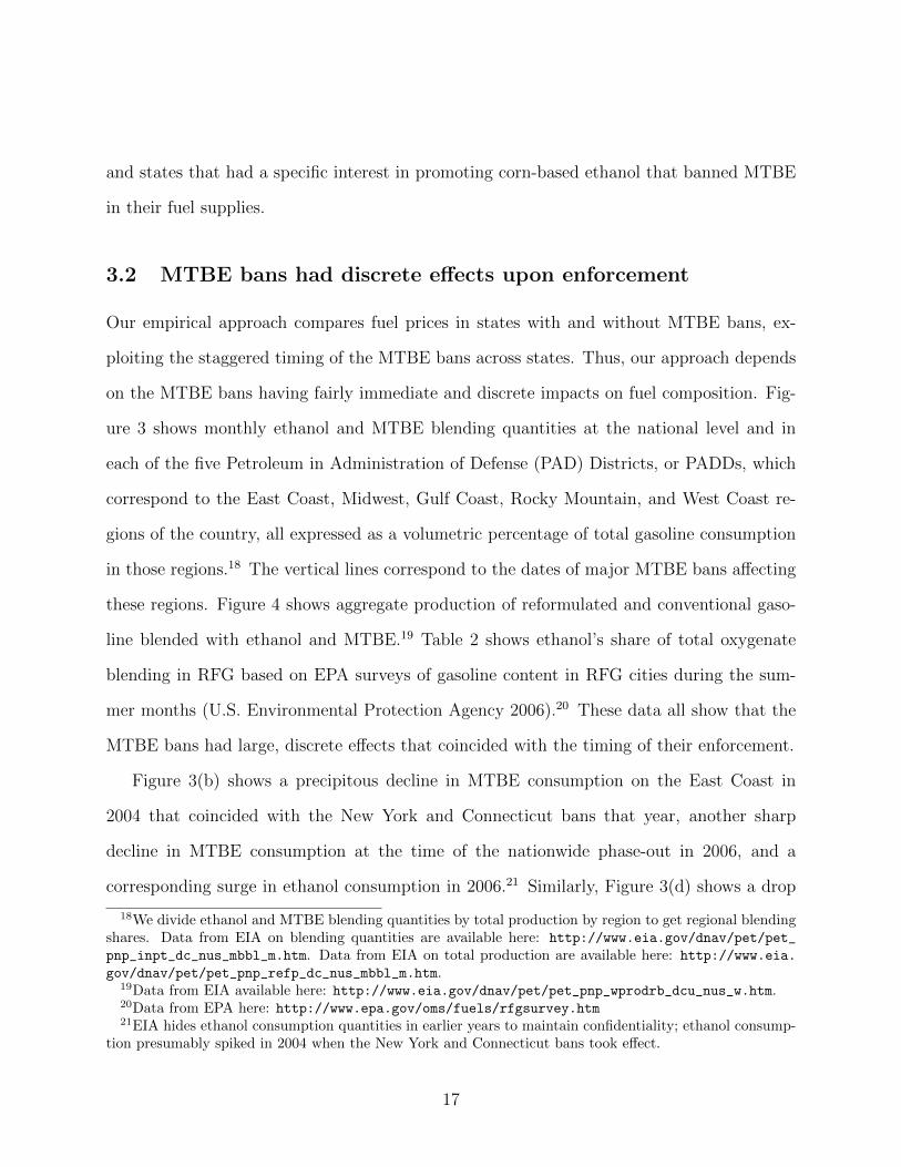
3.2 MTBE bans had discrete effects upon enforcement
Our empirical approach compares fuel prices in states with and without MTBE bans, ex-
ploiting the staggered timing of the MTBE bans across states. Thus, our approach depends
on the MTBE bans having fairly immediate and discrete impacts on fuel composition. Fig-
ure 3 shows monthly ethanol and MTBE blending quantities at the national level and in
each of the five Petroleum in Administration of Defense (PAD) Districts, or PADDs, which
correspond to the East Coast, Midwest, Gulf Coast, Rocky Mountain, and West Coast re-
gions of the country, all expressed as a volumetric percentage of total gasoline consumption
in those regions.18 The vertical lines correspond to the dates of major MTBE bans affecting
these regions. Figure 4 shows aggregate production of reformulated and conventional gaso-
line blended with ethanol and MTBE.19 Table 2 shows ethanol’s share of total oxygenate
blending in RFG based on EPA surveys of gasoline content in RFG cities during the sum-
mer months (U.S. Environmental Protection Agency 2006).20 These data all show that the
MTBE bans had large, discrete effects that coincided with the timing of their enforcement.
Figure 3(b) shows a precipitous decline in MTBE consumption on the East Coast in
2004 that coincided with the New York and Connecticut bans that year, another sharp
decline in MTBE consumption at the time of the nationwide phase-out in 2006, and a
corresponding surge in ethanol consumption in 2006.21 Similarly, Figure 3(d) shows a drop
18We divide ethanol and MTBE blending quantities by total production by region to get regional blendingshares. Data from EIA on blending quantities are available here: http://www.eia.gov/dnav/pet/pet_
pnp_inpt_dc_nus_mbbl_m.htm. Data from EIA on total production are available here: http://www.eia.
gov/dnav/pet/pet_pnp_refp_dc_nus_mbbl_m.htm.19Data from EIA available here: http://www.eia.gov/dnav/pet/pet_pnp_wprodrb_dcu_nus_w.htm.20Data from EPA here: http://www.epa.gov/oms/fuels/rfgsurvey.htm21EIA hides ethanol consumption quantities in earlier years to maintain confidentiality; ethanol consump-
tion presumably spiked in 2004 when the New York and Connecticut bans took effect.
17

Figure 3: Ethanol and MTBE blending quantities by region
(a) United States0
.02
.04
.06
.08
.1.1
2
Frac
tion
1994m1 1997m1 2000m1 2003m1 2006m1 2009m1
Month
MTBE share
Ethanol share
(b) East Coast (PADD 1)
0.0
2.0
4.0
6.0
8.1
.12
Frac
tion
1994m1 1997m1 2000m1 2003m1 2006m1 2009m1
Month
MTBE share
Ethanol share
(c) Midwest (PADD 2)
0.0
2.0
4.0
6.0
8.1
.12
Frac
tion
1994m1 1997m1 2000m1 2003m1 2006m1 2009m1
Month
MTBE share
Ethanol share
(d) South (PADD 3)
0.0
2.0
4.0
6.0
8.1
.12
Frac
tion
1994m1 1997m1 2000m1 2003m1 2006m1 2009m1
Month
MTBE share
Ethanol share
(e) Rocky Mountain (PADD 4)
0.0
2.0
4.0
6.0
8.1
.12
Frac
tion
1994m1 1997m1 2000m1 2003m1 2006m1 2009m1
Month
MTBE share
Ethanol share
(f) West Coast (PADD 5)
0.0
2.0
4.0
6.0
8.1
.12
Frac
tion
1994m1 1997m1 2000m1 2003m1 2006m1 2009m1
Month
MTBE share
Ethanol share
Note: These figures show monthly ethanol and MTBE volumetric blending shares by U.S.
Petroleum Administration for Defense District (PADD). Vertical lines correspond to California’s
initial MTBE ban and Kentucky’s phase-out (January 2003), bans in California, Connecticut,
New York, and Washington (January 2004), and the nationwide ban (May 2006) for the regions
in which these policy changes were active. See text for details.
18

Table 2: Ethanol market shares in Reformulated Gasoline, Summers 1999–2006
Area 1998 1999 2000 2001 2002 2003 2004 2005 2006MIDWEST
Chicago, IL-Gary, IN 96 100 100 100 100 100 100 100 100
Milwaukee-Racine, WI 97 100 100 100 100 100 100 100 100
St. Louis, MO 20 13 15 98 97 99 100 100
Louisville, KY 30 24 21 26 19 100 100 100 100
Covington, KY 46 75 67 66 67 100 100 100 100
EAST COASTKnox-Lincoln Co, MELewiston-Auburn, ME 0Portland, ME 0
Manchester, NH 0 0 0 0 0 0 0 0 100
Portsmouth-Dover, NH 0 0 0 0 0 0 0 0 100
Springfield, MA 0 0 0 0 0 0 3 24 100
Boston-Worcester, MA 0 0 0 0 0 0 0 3 100
Poughkeepsie, NY 0 0 0 0 0 0 98 100 100
NYC-Long Island, NY-NJ-CT 0 0 0 0 0 0 54 56 100
Hartford, CT 0 0 0 0 0 0 99 100 100
Connecticut 0 0 0 99 100 100
Warren Co, NJ 0 0 0 0 0 100
Atlantic City, NJ 0 0 0 0 0 0 0 100
Rhode Island 0 0 0 0 0 0 0 3 100
Sussex Co, DE 0 0 0 0 0 0 0 99
Philadelphia, PA 0 0 0 0 0 0 0 0 100
Baltimore, MD 0 0 0 0 0 0 0 0 96
Queen Anne-Kent Co, MD 0 0 0 0 93
Washington, DC 0 0 0 0 0 0 0 0 100
Norfolk-Virginia Beach, VA 0 0 0 0 0 0 0 0 99
Richmond, VA 0 0 0 0 0 0 0 0 100
GULF COAST
Dallas-Forth Worth, TX 0 0 0 0 0 0 0 0 99
Houston-Galveston, TX 0 0 0 0 0 0 0 0 100
WEST COASTPhoenix, AZ
Los Angeles, CA 0 0 0 7 9 93 100 100
Sacramento, CA 0 0 0 6 7 41 100 100
San Diego, CA 0 0 0 4 5 65 100 100
San Joaquin, CA 32 100 100
Note: This table reports ethanol’s summer market share in RFG by year and region, expressed as a percentage
of average oxygenate content (ethanol plus MTBE, by weight) that comes from ethanol. Market shares are
also available for winter months, but it is unclear whether the winter samples were collected prior to the
summer or afterwards, since winter collection dates vary but are not reported. Thus, for consistency, and
to ensure proper ordering in time, we only show summer ethanol market shares. The boxes denote location
and timing of samples affected by new MTBE bans. All bans are state bans, with the exception of Chicago’s
city ban in 2001. Note that California’s ban initially was to begin in January 2003. See text for details.19

in MTBE consumption in the South and corresponding increase in ethanol consumption in
2006. Figure 3(f) shows a precipitous decline in MTBE consumption on the West Coast that
coincided with the California ban in 2003–2004.22 Table 2 confirms these patterns of ethanol
and MTBE consumption in RFG for the East Coast, the South (namely, Texas), and the
West Coast.
Figure 3(c) shows a surprising increase in ethanol consumption in the Midwest in 2002–
2003, since no bans affecting RFG areas took effect that year.23 Table 2 shows that RFG
suppliers in Kentucky and Missouri (both located in the Midwest PADD) switched from
MTBE to ethanol in 2002–2003. While MTBE bans in these states took effect in 2005 and
2006, the bans were enacted in the summer of 2002.24 In addition, Michigan’s MTBE ban in
2003 also likely played a role. Michigan had no RFG, but ethanol and MTBE are also valued
as octane boosters. In any case, most Midwestern states were already using ethanol prior to
when their MTBE bans took effect. Thus, it will be important in our empirical analysis to
distinguish the Midwest from the rest of the country where the MTBE bans were actually
binding.
Figures 3 and 4 show a marked rise in ethanol blending beyond 2007, even though the
industry had had all but eliminated MTBE from gasoline by this time. The likely reason is
that the federal RFS had begun to bind, creating incentives to blend ethanol beyond what
earlier regulations required. Beyond 2007, it is clear that ethanol consumption is rising above
the level necessary to replace the banned MTBE. A binding federal RFS will tend to increase
national gasoline prices, while diminishing the shadow cost of an individual state’s MTBE
22California’s ban was originally scheduled to take effect in 2003, with several gasoline suppliers committingto eliminate MTBE that year. The ban was then delayed until 2004 and some suppliers waited (ExecutiveDepartment State of California 2002). Table 2 shows that the Los Angeles area nearly eliminated MTBE in2003, while other areas cut their MTBE consumption roughly in half, and that all areas in California hadswitched to ethanol by 2004.
23While Minnesota increased its explicit ethanol blending requirement from 2.7% to 10% in 2003, the statewas already subject to a year-round oxygenation requirement and MTBE ban. Thus, as far as we can tell,Minnesota’s policy change in 2003 should have had little effect on ethanol blending.
24Besides the MTBE bans, low ethanol prices around this time would have created fairly strong incentivesto boost volumes using ethanol as a direct gasoline substitute in regular gasoline, and the Midwest was in aposition to do so, given that it already had ethanol distribution and blending infrastructure.
20

Figure 4: Gasoline production
02
46
810
1214
Wee
kly
prod
uctio
n (m
illio
n B
BL/
day)
Mar05 Jul06 Nov07 Apr09 Aug10Date
Total
Conventional with ethanol
Reformulated with ethanol
Reformulated with MTBE
Note: This figure shows weekly U.S. production of gasoline, conventional gasoline
blended with ethanol, reformulated gasoline blended with ethanol, and reformu-
lated gasoline blended with MTBE. See text for details.
ban or ethanol mandate relative to gasoline prices in other states. Thus, we suspect that a
binding RFS pushes the estimated impacts of state-level MTBE bans toward zero.
4 Econometric models and estimation results
In this section we present our econometric analyses for retail gasoline prices. We begin
by estimating the impact of MTBE bans on average gasoline price levels by state. We then
estimate the impact of the bans on the monthly pass-through rates for key commodity inputs,
including crude oil, ethanol, and MTBE.
21
4.1 Data sources
We obtain monthly, state-level data on pre-tax retail gasoline prices from the U.S. Energy
Information Administration (EIA). These data report average prices for reformulated and
conventional gasoline.25 We express these and all other prices in January 2009 dollars using
the Consumer Price Index (all goods, urban consumers) from the Bureau of Labor Statistics.
In our econometric analysis below, we focus on the years 1996–2009—a period that covers
all state MTBE bans and during which other major fuel regulations that affected oxygenate
blending remained largely unchanged.
We obtain monthly crude oil prices from the EIA. These data measure national average
prices paid by domestic refiners for imported crude oil.26 We obtain monthly ethanol prices
from the State of Nebraska Energy Office, which measure monthly wholesale rack prices in
Omaha, Nebraska.27 We obtain weekly data on wholesale MTBE prices from Platt’s, which
measure wholesale rack prices on the U.S. Gulf Coast. We used these data to calculate
monthly average prices.
Table 3 presents summary statistics for these price variables.
4.2 Gasoline price levels
We estimate the effects of MTBE bans on average pre-tax retail gasoline price levels using
the following econometric equation:
pricejst = αjt · banjst + δjs + θt + εjst, (1)
25Available here: http://www.eia.gov/dnav/pet/pet_pri_allmg_a_EPM0_PTA_dpgal_m.htm. Conven-tional gasoline includes winter oxygenated gasoline in cities and time periods subject to such regulation.While price data for winter oxygenated gasoline areas are also reported separately, these data include manymissing observations. In addition, the specific cities and time periods subject to winter oxygenation changeover time, conflating changes in gasoline content regulations with changes in seasonality and geography.
26Available here: http://tonto.eia.doe.gov/dnav/pet/pet_pri_rac2_dcu_nus_m.htm.27Available here: http://www.neo.ne.gov/statshtml/66.html. We also obtained weekly data on whole-
sale rack prices for several-dozen individual U.S. cities for 1996–2008. Monthly average prices based on thissample of cities closely align with the Nebraska series, which is publicly available for the entire sample period.
22

Table 3: Summary statistics
Variable Mean Std.Dev. Observationspriceconventional 1.56 0.62 7225pricerfg 1.58 0.61 2971pricewholesale 1.54 0.61 8364priceoil 0.97 0.53 8415priceethanol 1.19 0.53 8415pricemtbe 1.46 0.59 7599
Note: This table reports summary statistics for the retail gasoline and wholesale input prices used
in the estimation. All prices are in real 2010 dollars per gallon. See text for details.
where pricejst is the average price of gasoline sold in state j in season s at time t. The policy
variable of interest is banjst, which is a dummy variable indicating whether a given state is
subject to an MTBE ban in a given month, including both state bans as well as the implicit
nationwide ban for all states starting in May 2006 and onwards. The coefficient of interest is
αjt, which measures the effect of the MTBE ban on average gasoline prices. The variable δjs
is a state-season (e.g., Michigan-July) effect that controls for persistent differences in average
prices across states and seasons, including seasonality in local gasoline content regulations.
The variable θt is a time effect that controls for time trends that are constant across states.
Lastly, εjst is an error term that we assume is uncorrelated with the MTBE bans.
We have reason to believe that the effect of an MTBE ban will vary over time t and across
locations j. For example, MTBE bans will likely have milder effects on gasoline prices in
the Midwest, while MTBE bans could raise average prices dramatically when ethanol prices
are high. Thus, we allow αjt to vary for Midwestern and non-Midwestern states and with
input prices for crude oil, ethanol, and MTBE. In our most general and favored model, the
impact of an MTBE ban on gasoline prices takes the form:
αjt = β0 + β1 ·Midwestj +∑input
(βinput + γinput ·Midwestj) · priceinput,t, (2)
where Midwestj is a dummy variable indicating whether a state is in the Midwest PADD
23

and priceinput is the wholesale price of a particular gasoline input—crude oil, ethanol, or
MTBE—less its sample mean (reported in Table 3). Thus, we can interpret α0 as the effect
of an MTBE ban on gasoline prices outside of the Midwest when crude oil, ethanol, and
MTBE prices equal their sample-mean values, while β0 + β1 is the corresponding effect in
the Midwest. The summation term then allows these effects to vary as input prices deviate
from their sample-mean values.28
We estimate equation (1) separately for conventional gasoline (which includes winter
oxygenated fuel in affected areas) and RFG using OLS. The key identification assumption
is that the timing of the MTBE bans is uncorrelated with state trends in state gasoline
prices. This is a reasonable assumption given that bans were driven primarily by concerns
about groundwater contamination and support for the ethanol industry, rather than in re-
sponse to fuel prices, and were enacted months or years before they became effective. We
estimate Newey-West standard errors, which are robust to both heteroskedasticity and serial
correlation.29
Table 4 presents the results. Focusing on column (4), the coefficients on ban and on
ban ×midwest indicate that the MTBE bans had virtually no effect on gasoline prices for
conventional gasoline, either in the Midwest or elsewhere, when evaluated sample mean oil,
ethanol, and MTBE input prices. All else equal, however, a $1 increase in ethanol input
prices increases the impact of the MTBE ban by about 3.4 cents per gallon outside of the
Midwest, as indicated by the coefficient on ban × priceethanol. All else equal, a $1 increase
in MTBE input prices decreases the impact of the MTBE ban by about 5.7 cents per gallon
outside of the Midwest, as indicated by the coefficient on ban × pricemtbe. The negative
28Since an MTBE ban in one state could potentially affect gasoline prices in a different state indirectly vianational wholesale markets for fuel inputs, these interactions are also important for identifying all-else-equaleffects in the presence of general-equilibrium spillovers.
29We regressed the OLS residuals on their lagged values after one month, two months, and so on. Wefound these autocorrelations to be significant for lag lengths as long as seven months. Thus, we use aseven-month lag when calculating our Newey-West standard errors. To test the robustness of our standarderror estimates, we also varied the lag length from 3 to 11 months. While estimated standard errors tendedto increase with longer lag lengths, the increase was so slight that it did not meaningfully affect precisionrelative to the magnitude of our point estimates.
24

Table 4: Main estimation results: gasoline price levels (dollars)
Coefficient Conventional gasoline Reformulated gasoline(1) (2) (3) (4) (5) (6) (7) (8)
ban 0.014** 0.017** 0.006 0.007 0.013 0.017 0.044*** 0.059***(0.007) (0.008) (0.006) (0.011) (0.010) (0.011) (0.014) (0.015)
ban× priceoil -0.084** -0.041 -0.041 -0.003(0.034) (0.040) (0.058) (0.060)
ban× priceethanol 0.020 0.034** -0.012 0.003(0.013) (0.017) (0.019) (0.020)
ban× pricemtbe 0.003 -0.057** -0.037** -0.078***(0.015) (0.025) (0.018) (0.023)
ban×midwest -0.005 0.002 -0.012 -0.048***(0.007) (0.011) (0.009) (0.017)
ban×midwest× priceoil -0.051** 0.013(0.025) (0.031)
ban×midwest× priceethanol -0.021** -0.044***(0.010) (0.015)
ban×midwest× pricemtbe 0.077*** 0.072***(0.021) (0.025)
Observations 7225 7225 6527 6527 2971 2971 2684 2684
Note: This table reports main estimation results. Dependent variable is the average real price of gasoline(either conventional or reformulated) in a given state and month in real 2010 dollars. All regressions controlfor month effects (e.g., November 2004) and state-season (e.g., Massachusetts-March) effects. Standarderrors in parentheses are robust to serial correlation and heteroskedasticity (Newey-West standard errorswith a seven-month lag).
coefficients on ban × midwest × priceethanol and ban × midwest × pricemtbe indicate that
these impacts are considerably smaller in the Midwest, which makes sense, given that the
Midwest would not have been consuming much MTBE prior to the bans anyway. Higher
crude oil prices have a statistically insignificant effect on the ban’s impact.
Moving now to column (8), which reports results for RFG, we should expect to see a
similar pattern of coefficients. The magnitudes should be larger, however, reflecting the fact
that all producers of RFG were required to blend either ethanol or MTBE prior to 2006
and had little flexibility to do otherwise, even after the oxygenation requirement for RFG
was removed, given other constraints. The coefficient on ban indicates that the MTBE bans
increased prices for RFG by 5.9 cents outside of the Midwest, assuming sample-mean input
prices.30 The impact on prices in the Midwest is not statistically different from zero. It
30These results are consistent with Brown et al. (2008) who find that RFG regulations increased wholesalegasoline prices in select Midwestern cities by 4–9 cents more than on the coasts, mainly reflecting higherrefining costs for the ethanol-ready RFG blendstock used in the Midwest. Our higher estimates for retailgasoline in coastal states reflect both these higher refining costs, as well as the add-on costs for ethanoltransportation and blending.
25

is not surprising that these impacts are bigger for RFG than for conventional fuel, since
RFG requires oxygenate blending, either directly or indirectly—as the lowest-cost approach
to meeting other RFG performance standards—and because blending ethanol with RFG
requires that refiners significantly reduce the RVP of the underlying gasoline blendstock.
Again, these impacts depend on input prices. Strangely, higher ethanol prices do not
increase the impact of the ban, although higher ethanol prices decrease the impact of the
ban in the Midwest relative to other states, as expected. Higher MTBE prices strongly
reduce the impact of the MTBE ban outside of the Midwest, however, while having little
effect on the impact of a ban in the Midwest. These impacts are all higher for RFG than for
conventional fuel, which is not surprising, given the greater flexibility of conventional fuel
producers. The impact of a ban on RFG prices does not appear to be sensitive to crude oil
prices, controlling for other inputs.
In addition to these preferred models, the table also presents results for models that
restrict the impacts of MTBE bans to be the same for all states and time periods (columns
1 and 5), different across states but the same across time periods (columns 2 and 6), and
different across time periods but the same across states (columns 3 and 7). Two patterns
emerge. First, the estimated impact of an MTBE ban is smaller when imposing a constant
effect across all locations, which implies that it is important to differentiate the Midwest from
states for whom the MTBE bans were binding. Second, the estimated impact of an MTBE
ban declines in magnitude when not controlling for nationwide input prices. Apparently,
either the timing of the MTBE bans is correlated with wholesale input prices, or local retail
markets are connected via national input markets in ways that bias the coefficient estimates
toward zero.
26

4.3 Monthly pass-through rates for wholesale inputs
We now estimate how MTBE bans alter monthly pass-through rates for wholesale input
costs using the following econometric equation:
∆pricejst =∑input
(βinput + γinput ·Midwestj) · banjst ·∆priceinput,t + δjs + θt + ∆εjst, (3)
where ∆pricejst is the monthly change in gasoline prices in state j in season s at time t. The
variables of interest are interactions between the state MTBE bans and monthly changes in
the various input prices, given by banjst ·∆priceinput,t. Thus, the corresponding coefficients
given by βinput +γinput ·Midwestj measure changes in input pass-through rates when a state
imposes an MTBE ban. As before, these effects are allowed to differ regionally through an
additional interaction with Midwestj. Of the remaining terms, δjs is a state-season effect
that allows retail prices to follow different time trends by state and season in this first-
differenced model, θt is a month effect, and ∆εjst is an error term. Note that the month
effects prevent us from estimating pass-through rates directly, given that our input price
data do not vary across states; we are only able to estimate changes in pass-through rates.
Also note that we have omitted the direct effects of the bans, since the changeovers from
MTBE to ethanol in response to state bans, while rapid, typically occurred over the span
of several months leading up to the enforcement dates, with the exact timing varying from
state to state. Thus, the direct effect on prices would be unlikely to show up in monthly
first-differenced data.
As above, we estimate equation (3) separately for conventional gasoline and RFG using
OLS. Here, the key identification assumption is that the monthly change in gasoline prices
in a state is uncorrelated with the timing of its MTBE ban after controlling for linear state-
season trends, which is a weaker assumption than before.
Table 5 presents our results. Focusing on column (2), the coefficient on ban× priceethanol
indicates that an MTBE ban increases the monthly pass-through rate for ethanol prices by
27

Table 5: Main estimation results: gasoline price first differences (dollars)
Coefficient Conventional gasoline Reformulated gasoline(1) (2) (3) (4)
ban×∆priceoil 0.098** 0.010 -0.035 -0.072(0.042) (0.045) (0.088) (0.084)
ban×∆priceethanol -0.011 0.046*** -0.051* 0.008(0.015) (0.018) (0.029) (0.027)
ban×∆pricemtbe 0.029* -0.086*** -0.056** -0.121***(0.016) (0.018) (0.025) (0.024)
ban×midwest×∆priceoil 0.133*** 0.079(0.031) (0.053)
ban×midwest×∆priceethanol -0.080*** -0.152***(0.014) (0.021)
ban×midwest×∆pricemtbe 0.151*** 0.157***(0.014) (0.024)
Observations 6454 6454 2657 2657
Note: This table reports main estimation results. Dependent variable is the monthly change in the average
real price of gasoline (either conventional or reformulated) in a given state and month in real 2010 dollars.
All regressions control for month effects (e.g., November 2004) and state-season (e.g., Massachusetts-March)
effects. Standard errors in parentheses are robust to serial correlation and heteroskedasticity (Newey-West
standard errors with a six-month lag).
0.046 outside of the Midwest, while decreasing the pass-through rate for MTBE prices by
0.086. In the Midwest, an MTBE ban does little to change the pass-through rate for ethanol
prices, as expected. Surprisingly, an MTBE ban in the Midwest increases the pass-through
rate for MTBE prices by −0.086 + 0.151 = 0.065 and increases the monthly pass-through
for crude oil prices by 0.010 + 0.133 ≈ 0.143.
Now focusing on column (4), the coefficient on ban×priceethanol indicates that the MTBE
ban unexpectedly does little to change the monthly pass-through of wholesale ethanol prices
to retail RFG prices outside of the Midwest, while the coefficient on ban×pricemtbe indicates
that the ban decreases the pass-through of wholesale MTBE prices by 0.121, which is what
we would have expected. In the Midwest, the MTBE ban unexpectedly decreases the pass-
through of ethanol prices while having little effect on the pass-through of MTBE or crude oil
prices, as expected. Overall, however, the results are consistent with our conceptual model
above. The MTBE bans generally increase the monthly pass-through of ethanol prices and
28

decrease the monthly pass-through of MTBE prices outside of the Midwest, while having
little effect on the pass-through of crude oil prices. In the Midwest, the ban’s effects either
tend to zero or have the opposite sign as in other regions.
In addition to these preferred models, the table also presents results for models that
restsrict the effects to be identical across states (columns 1 and 3). As expected, imposing
coefficients that are equivalent across states tends to reduce their magnitudes, which again
implies that it is important to differentiate between the Midwest and the rest of the country.
4.4 Late enforcement of MTBE bans
A total of six states enacted MTBE bans that took effect subsequent to the nationwide phase-
out in the spring of 2006. In principle, these bans should have had no effect on gasoline price
levels or input price pass-through rates, given the nationwide phase-out. This is a testable
hypothesis. Thus, we create a second policy variable, called latebanjst, which equals one
for states whose bans took effect after May 2006, in the months these “late” bans were in
effect, and zero otherwise. We then repeat each of our previous regressions, including both
latebanjst and its interactions with wholesale input prices as additional controls. There is no
need to differentiate this policy variable by location, however, since every state with a late
MTBE ban was located outside of the Midwest.
Table 6 presents the results for gasoline price levels. We find that the individual coeffi-
cients on the late ban variables are generally small and statistically insignificant. Along the
bottom of the table, we present the P-values for Wald tests of the joint significance of the
lateban variables. In our preferred models in columns (4) and (8), the late MTBE bans are
only borderline significant at the 8% and 16% levels. Overall, these results are consistent
with our identification assumption above that the state MTBE bans were not timed in a
way that correlated with gasoline prices, conditional on controls.
Table 7 presents the corresponding results for the impact of MTBE bans on pass-through
rates for wholesale input prices. Here, the results are somewhat less rosy. While most
29

coefficients are again statistically insignificant, the interactions with ethanol prices are large
and significant, and the P-values for the joint tests are quite small. One possible explanation
is that since the nationwide phase-out was not a literal ban, MTBE is in fact used in some
rare circumstances when other options are quite costly. In any case, these late bans only
occur in four RFG locations, including Maine, New Hampshire, New Jersey, and Rhode
Island.
5 Conclusion
We estimate the impacts of MTBE bans on gasoline prices. While interesting in their own
right, these bans approximate direct ethanol blending mandates in areas that require oxy-
genate blending. Thus, these bans help us learn about the potential effects of renewable
fuel blending mandates on gasoline prices. We find that MTBE bans increased RFG prices
by 6 cents per gallon in areas where the bans were binding. The impacts of a ban would
have been bigger had ethanol prices been higher or had MTBE prices been lower. These
results represent the first rigorous empirical confirmation of the theoretical result that a
percent ethanol blending mandate will inevitably increase fuel prices in a competitive mar-
ket when the ethanol supply curve is more steeply sloped than that of gasoline—with the
obvious qualification that this inference is based on a surrogate policy with similar economic
structure.
There are several important caveats to our results and their interpretation. First, we
have identified the effects of the MTBE bans on consumers through retail prices. A more
complete welfare analysis would obviously require information on producer costs, as well as
information on the potential health benefits to those not exposed to environmental contam-
ination. Second, we only present reduced-form impacts on retail prices during the era of the
MTBE bans. While we partially decompose these effects according to prices for wholesale
inputs, the effects could look different in the long run, as new ethanol blending infrastructure
30

is added, or under substantially different market conditions. Third, while we have shown
qualitatively that a state MTBE ban can approximate a state ethanol mandate under certain
conditions, the two policies are not identical. Moreover, the shapes of the ethanol and gaso-
line supply curves to a particular state could look quite different from the shapes of national
supply. Thus, while a state ethanol mandate might have qualitatively similar effects to a
national RFS, the precise magnitudes would likely differ considerably.
References
Anderson, Soren T., “The Demand for Ethanol as a Gasoline Substitute,” Journal of
Environmental Economics and Management, 2012, 63 (2), 151–168.
Auffhammer, Maximilian and Ryan Kellogg, “Clearing the Air? The Effects of Gaso-
line Content Regulation on Air Quality,” American Economic Review, 2011, 101 (6),
2687–2722.
Brown, Jennifer, Justine Hastings, Erin T. Mansur, and Sofia B. Villas-Boas, “Re-
formulating Competition? Gasoline Content Regulation and Wholesale Gasoline Prices,”
Journal of Environmental Economics and Management, 2008, 55 (1), 1–19.
Chakravorty, Ujjayant, Cline Nauges, and Alban Thomas, “Clean Air Regulation
and Heterogeneity in U.S. Gasoline Prices,” Journal of Environmental Economics and
Management, 2008, 55 (1), 106–122.
Chouinard, Hayley H. and Jeffrey M. Perloff, “Gasoline Price Differences: Taxes,
Pollution Regulations, Mergers, Market Power, and Market Conditions,” The B.E. Journal
of Economic Analysis & Policy, 2007, 7 (1), 8.
Executive Department State of California, “Executive Order D-52-02,” March 2002.
31

Holland, Stephen P., Christopher R. Knittel, and Jonathan E. Hughes, “Green-
house Gas Reductions Under Low Carbon Fuel Standards?,” American Economic Journal:
Economic Policy, 2008, 1 (1), 106–146.
Hughes, Jonathan E., “The Higher Price of Cleaner Fuels: Market Power in the Rail
Transport of Fuel Ethanol,” Journal of Environmental Economics and Management, 2011,
62 (2), 123–139.
, Christopher R. Knittel, and Daniel Sperling, “Evidence of a Shift in the Short-Run
Price Elasticity of Gasoline Demand,” The Energy Journal, January 2008, 29 (1).
Knittel, Christopher R. and Aaron Smith, “Ethanol Production and Gasoline Prices:
A Spurious Correlation,” July 2012. UC Center for Energy and Environmental Economics
Working Paper WP-043.
Lidderdale, Trancred C., “MTBE Production Economics,” April
2001. U.S. Energy Information Administration, Available at:
http://www.eia.doe.gov/steo/special/mtbecost.html.
Muehlegger, Erich J., “Gasoline Price Spikes and Regional Gasoline Content Regulations:
A Structural Approach,” March 2006.
Salvo, Alberto and Cristian Huse, “Build It, But Will They Come? Evidence From
Consumer Choice Between Gasoline and Sugarcane Ethanol,” May 2012. Working Paper.
Small, Kenneth A. and Kurt Van Dender, “Fuel Efficiency and Motor Vehicle Travel:
The Declining Rebound Effect,” Energy Journal, 2007, 28 (1), 25–51.
Stikkers, David E., “Octane and the Environment,” Science of The Total Environment,
2002, 299 (1-3), 37–56.
Trench, C.J., “How Pipelines Make the Oil Market Work—Their Networks, Operation and
Regulation,” 2001.
32

U.S. Energy Information Administration, “Status and Impact of State MTBE Bans,”
March 2003. Available at: http://www.eia.doe.gov/oiaf/servicerpt/mtbeban/index.html.
U.S. Enviornmental Protection Agency, “State Actions Banning MTBE (Statewide),”
August 2007.
U.S. Environmental Protection Agency, “RFG Properties Survey Data,” 2006. Avail-
able at: http://www.epa.gov/otaq/regs/fuels/rfg/properf/rfgperf.htm.
Weaver, James W., Linda R. Exum, and Lourdes M. Prieto, “Gasoline Composition
Regulations Affecting LUST Sites,” January 2010. U.S. Environmental Protection Agency.
33

Table 6: Late bans: gasoline price levels (dollars)
Coefficient Conventional gasoline Reformulated gasoline(1) (2) (3) (4) (5) (6) (7) (8)
ban 0.013** 0.015* 0.006 0.007 0.013 0.018* 0.044*** 0.059***(0.007) (0.009) (0.006) (0.017) (0.010) (0.011) (0.014) (0.015)
ban× priceoil -0.084** -0.044 -0.041 -0.002(0.034) (0.041) (0.058) (0.060)
ban× priceethanol 0.020 0.035** -0.012 0.003(0.013) (0.017) (0.019) (0.020)
ban× pricemtbe 0.003 -0.057** -0.037** -0.078***(0.015) (0.026) (0.018) (0.023)
ban×midwest -0.003 0.002 -0.013 -0.050***(0.007) (0.011) (0.010) (0.017)
ban×midwest× priceoil -0.047* 0.015(0.026) (0.032)
ban×midwest× priceethanol -0.023** -0.044***(0.010) (0.015)
ban×midwest× pricemtbe 0.077*** 0.072***(0.022) (0.025)
lateban 0.024*** 0.023** -0.006 -0.006 -0.007 -0.010 -0.044 -0.057**(0.009) (0.010) (0.022) (0.023) (0.009) (0.009) (0.028) (0.028)
lateban× priceoil 0.041 0.024 0.019 0.023(0.029) (0.031) (0.037) (0.038)
lateban× priceethanol 0.014 0.005 -0.001 -0.016(0.032) (0.032) (0.035) (0.034)
lateban× pricemtbe -0.021 0.008 0.015 0.038(0.038) (0.039) (0.046) (0.044)
Observations 7225 7225 6527 6527 2971 2971 2684 2684P-value 0.006 0.016 0.117 0.080 0.435 0.251 0.439 0.157
Note: This table reports results for the “late” state MTBE bans that took effect subsequent to the na-tionwide ban in May 2006. Dependent variable is the average real price of gasoline (either conventional orreformulated) in a given state and month in real 2010 dollars. All regressions control for month effects (e.g.,November 2004) and state-season (e.g., Massachusetts-March) effects. Standard errors in parentheses arerobust to serial correlation and heteroskedasticity (Newey-West standard errors with a seven-month lag).P-value in the bottom row is the Wald test P-value for the null hypothesis that the coefficients on all latebanvariables are jointly zero.
34

Table 7: Late bans: gasoline price first differences (dollars)
Coefficient Conventional gasoline Reformulated gasoline(1) (2) (3) (4)
ban×∆priceoil 0.098** 0.006 -0.035 -0.074(0.042) (0.045) (0.088) (0.084)
ban×∆priceethanol -0.011 0.045** -0.050* 0.008(0.015) (0.018) (0.029) (0.027)
ban×∆pricemtbe 0.029* -0.088*** -0.056** -0.122***(0.016) (0.018) (0.025) (0.024)
ban×midwest×∆priceoil 0.138*** 0.081(0.031) (0.054)
ban×midwest×∆priceethanol -0.079*** -0.151***(0.014) (0.021)
ban×midwest×∆pricemtbe 0.153*** 0.159***(0.014) (0.024)
lateban 0.006 0.006 0.008 0.009(0.006) (0.006) (0.005) (0.005)
lateban×∆priceoil -0.025 0.025 -0.040 -0.017(0.071) (0.073) (0.053) (0.055)
lateban×∆priceethanol 0.102*** 0.071* 0.102*** 0.057(0.039) (0.038) (0.037) (0.035)
lateban×∆pricemtbe -0.020 0.037 -0.026 0.023(0.031) (0.030) (0.032) (0.030)
Observations 6454 6454 2657 2657Placebo test P-value 0.046 0.000 0.013 0.016
Note: This table reports results for the “late” state MTBE bans that took effect subsequent to the nationwide
ban in May 2006. Dependent variable is the monthly change in the average real price of gasoline (either
conventional or reformulated) in a given state and month in real 2010 dollars. All regressions control for
month effects (e.g., November 2004) and state-season (e.g., Massachusetts-March) effects. Standard errors in
parentheses are robust to serial correlation and heteroskedasticity (Newey-West standard errors with a six-
month lag). P-value in the bottom row is the Wald test P-value for the null hypothesis that the coefficients
on all lateban variables are jointly zero.
35