arX

iv:1

507.

0277

2v2

[cs.

CV

] 17

Dec

201

51

Riemannian Dictionary Learning and SparseCoding for Positive Definite Matrices

Anoop Cherian Suvrit Sra

Abstract—Data encoded as symmetric positive definite(SPD) matrices frequently arise in many areas of computervision and machine learning. While these matrices form anopen subset of the Euclidean space of symmetric matrices,viewing them through the lens of non-Euclidean Riemanniangeometry often turns out to be better suited in capturingseveral desirable data properties. However, formulating clas-sical machine learning algorithms within such a geometry isoften non-trivial and computationally expensive. Inspired bythe great success of dictionary learning and sparse coding forvector-valued data, our goal in this paper is to represent datain the form of SPD matrices as sparse conic combinationsof SPD atoms from a learned dictionary via a Riemanniangeometric approach. To that end, we formulate a novelRiemannian optimization objective for dictionary learning andsparse coding in which the representation loss is characterizedvia the affine invariant Riemannian metric. We also present acomputationally simple algorithm for optimizing our model .Experiments on several computer vision datasets demonstratesuperior classification and retrieval performance using ourapproach when compared to sparse coding via alternativenon-Riemannian formulations.

Index Terms—Dictionary learning, Sparse coding, Rieman-nian distance, Region covariances

I. I NTRODUCTION

SYMMETRIC positive definite (SPD) matrices play animportant role as data descriptors in several computer

vision applications, for example in the form of regioncovariances [1]. Notable examples where such descriptorsare used include object recognition [2], human detectionand tracking [3], visual surveillance [4], 3D object recog-nition [5], among others. Compared with popular vectorspace descriptors, such as bag-of-words, Fisher vectors,etc., the second-order structure offered by covariance ma-trices is particularly appealing. For instance, covariancesconveniently fuse multiple features into a compact formindependent of the number of data points. By choosingappropriate features, this fusion can be made invariant toaffine distortions [6], or robust to static image noise andillumination variations. Moreover, generating these descrip-tors is easy, for instance using integral image transforms [3].

We focus on SPD matrices for dictionary learning withsparse coding (DLSC) – a powerful data representation toolin computer vision and machine learning [7] that enablesstate-of-the-art results for a variety of applications [8], [9].

Anoop Cherian is with the ARC Centre of Excellence for RoboticVision, Australian National University, Canberra, Australia Email:anoop.cherian@anu.edu.au.

Suvrit Sra is with the Massachusetts Institute of Technology.E-mail: suvrit@mit.edu

Fig. 1. An illustration of our Riemannian dictionary learning andsparse coding. For the SPD manifoldM and learned SPD basismatricesBi on the manifold, our sparse coding objective seeks anon-negative sparse linear combination

∑

iαiBi of theBi’s that

is closest (in a geodesic sense) to the given input SPD matrixX.

Given a training set, traditional (Euclidean) dictionarylearning problem seeks an overcomplete set of basis vectors(the dictionary) that can be linearly combined to sparselyrepresent each input data point; finding a sparse repre-sentation given the dictionary is termedsparse coding.While sparse coding was originally conceived for Euclideanvectors, there have been recent extensions of the setup toother data geometries, such as histograms [10], Grassman-nians [11], and SPD matrices [12], [13], [14], [15]. Thefocus of this paper is on dictionary learning and sparsecoding of SPD matrix data using a novel mathematicalmodel inspired by the geometry of SPD matrices.

SPD matrices are an open subset of the Euclidean spaceof symmetric matrices. This may lead one to believe thatessentially treating them as vectors may suffice. However,there are several specific properties that applications us-ing SPD matrices demand. For example, in DT-MRI thesemidefinite matrices are required to be at infinite distancesfrom SPD matrices [16]. Using this and other geometricallyinspired motivation a variety of non-Euclidean distancefunctions have been used for SPD matrices—see e.g., [16],[17], [18]. The most widely used amongst these is the affineinvariant Riemannian metric [18], [19], the only intrinsicRiemannian distance that corresponds to a geodesic dis-tance on the manifold of SPD matrices.

In this paper, we study dictionary learning and sparsecoding of SPD matrices in their natural Riemannian geom-

2

etry. Compared to the Euclidean setup, their Riemanniangeometry, however, poses some unique challenges: (i) themanifold defined by this metric is (negatively) curved [20],and thus the geodesics are no more straight-lines; and (ii) incontrast to the Euclidean DLSC formulations, the objectivefunction motivated by the Riemannian distance is notconvex in either its sparse coding part or in the dictionarylearning part. We present some theoretical properties ofour new DLSC formulation and mention a situation ofpurely theoretical interest where the formulation is convex.Figure 1 conceptually characterizes our goal.

The key contributions of this paper are as follows.

• Formulation:We propose a new model to learn a dic-tionary of SPD atoms; each data point is representedas a nonnegative sparse linear combination of SPDatoms from this dictionary. The quality of the resultingrepresentation is measured by the squared intrinsicRiemannian distance.

• Optimization: The main challenge in using our for-mulation is its higher computational cost relative toEuclidean sparse coding. However, we describe a sim-ple and effective approach for optimizing our objectivefunction. Specifically, we propose a dictionary learn-ing algorithm on SPD atoms via conjugate gradientdescent on the product manifold generated by the SPDatoms in the dictionary.

A forerunner to this paper appeared in [21]. The currentpaper differs from our conference paper in the followingmajor aspects: (i) we propose a novel dictionary learningformulation and an efficient solver for it; and (ii) extensivenew experiments using our dictionary learning are alsoincluded and the entire experimental section re-evaluatedunder our new setup while also including other datasetsand evaluation metrics.

To set the stage for presenting our contributions, we firstreview key tools and metrics from Riemannian geometrythat we use to develop our ideas. Then we survey somerecent methods suggested for sparse coding using alterna-tive similarity metrics on SPD matrices. Throughout wework with real matrices; extension to Hermitian positivedefinite matrices is straightforward. The space ofd × dSPD matrices is denoted asSd+, symmetric matrices bySd, and the space of (real) invertible matrices byGL(d).By Log(X), for X ∈ S+, we mean the principal matrixlogarithm andlog |X | denotes the scalar logarithm of thematrix determinant.

II. PRELIMINARIES

We provide below a brief overview of the Riemanniangeometry of SPD matrices. A manifoldM is a set of pointsendowed with a locally-Euclidean structure. Atangentvector at P ∈ M is defined as the tangent to some curvein the manifold passing throughP . A tangent spaceTPMdefines the union of all such tangent vectors to all possiblesuch curves passing throughP ; the point P is termedthe foot of this tangent space. The dimensionality ofTPMis the same as that of the manifold. It can be shown that the

tangent space is isomorphic to the Euclidean space [22];thus, they provide a locally-linear approximation to themanifold at its foot.

A manifold becomes a Riemannian manifold if its tan-gent spaces are endowed with a smoothly varying innerproduct. The Euclidean space, endowed with the classicalinner product defined by the trace function (i.e., for twopoints X,Y ∈ Sd, 〈X,Y 〉 = Tr(XY )), is a Riemannianmanifold. Recall that an SPD matrix has the property thatall its eigenvalues are real and positive, and it belongs tothe interior of a convex self-dual cone. Since ford×d SPDmatrices, this cone is a subset of the1

2d(d+1)-dimensionalEuclidean space of symmetric matrices, the set of SPDmatrices naturally forms a Riemannian manifold under thetrace metric. However, under this metric, the SPD manifoldis notcomplete1. This is because, the trace metric does notenclose all Cauchy sequences originating from the interiorof the SPD cone [23].

A possible remedy is to change the geometry of themanifold such that positive semi-definite matrices (whichform the closure of SPD matrices for Cauchy sequences)are at an infinite distance to points in the interior of the SPDcone. This can be achieved by resorting to the the classi-cal log-barrier functiong(P ) = − log det(P ), popular inthe optimization community in the context of interior pointmethods [24]. The trace metric can be modified to the newgeometry induced by the barrier function by incorporatingthe curvature through its Hessian operator at pointP in thedirectionZ given byHP (Z) = g′′(P )(Z) = P−1ZP−1.The Riemannian metric atP for two pointsZ1, Z2 ∈ TPMis thus defined as:

〈Z1, Z2〉P = 〈HPZ1, Z2〉 = Tr(P−1Z1P−1Z2). (1)

There are two fundamental operations that one needs forcomputations on Riemannian manifolds: (i) the exponentialmap ExpP : Sd → Sd+; and (ii) the logarithmic mapLogP = Exp−1

P : Sd+ → Sd, whereP ∈ Sd+. The former

projects a symmetric point on the tangent space onto themanifold (termed aretraction), the latter does the reverse.Note that these maps depend on the pointP at which thetangent spaces are computed. In our analysis, we will bemeasuring distances assumingP to be the identity matrix,I, in which case we will omit the subscript.

Note that the Riemannian metric provides a measure forcomputing distances on the manifold. Given two points onthe manifold, there are infinitely many paths connectingthem, of which the shortest path is termed thegeodesic. Itcan be shown that the SPD manifold under the Riemannianmetric in (1) is non-positively curved (Hadamard manifold)and has a unique geodesic between every distinct pair ofpoints [25][Chap. 12], [26][Chap. 6]. ForX,Y ∈ Sd+, thereexists a closed form for thisgeodesic distance, given by

dR(X,Y ) =∥

∥

∥Log(X−1/2Y X−1/2)

∥

∥

∥

F, (2)

1A space is a complete metric space if allCauchy sequences areconvergent within that space.

3

whereLog is the matrix logarithm. It can be shown that thisdistance is invariant to affine transformations of the inputmatrices [19] and thus is commonly referred to as theAffineinvariant Riemannian metric. In the sequel, we will use (2)to measure the distance between input SPD matrices andtheir sparse coded representations obtained by combiningdictionary atoms.

III. R ELATED WORK

Dictionary learning and sparse coding of SPD matriceshas received significant attention in the vision communitydue to the performance gains it brings to the respectiveapplications [7], [12], [15]. Given a training datasetX , theDLSC problem seeks a dictionaryB of basis atoms, suchthat each data pointx ∈ X can be approximated by asparse linear combination of these atoms while minimizinga suitable loss function. Formally, the DLSC problem canbe abstractly written as

minB,θx∀x∈X

∑

∀x∈X

L(x,B, θx) + λSp(θx), (3)

where the loss functionL measures the approximationquality obtained by using the “code”θx, while λ regulatesthe impact of the sparsity penaltySp(θx).

As alluded to earlier, the manifold geometry hindersa straightforward extension of classical DLSC techniques(such as [27], [28]) to data points drawn from a manifold.Prior methods typically use surrogate similarity distancesthat bypass the need to operate within the intrinsic Rieman-nian geometry, e.g., (i) by adapting information geometricdivergence measures such as the log-determinant diver-gence or the Stein divergence, (ii) by using extrinsic metricssuch as the log-Euclidean metric, and (iii) by relying onthe kernel trick to embed the SPD matrices into a suitableRKHS. We briefly review each of these schemes below.Statistical measures:In [14] and [29], a DLSC frameworkis proposed based on the log-determinant divergence (Burgloss) to model the loss. For two SPD matricesX,Y ∈Sd+, this divergence has the following formdB(X,Y ) =Tr(XY −1) − log

∣

∣XY −1∣

∣ − d. Since this divergence actsas a base measure for the Wishart distribution [4]—a naturalprobability density on SPD matrices—a loss defined usingit is statistically well-motivated. The sparse coding formu-lation using this loss reduces to a MAX DET optimizationproblem [14] and is solved using interior-point methods.Unsurprisingly, the method is often seen to be computa-tionally demanding even for moderately sized covariances(more than5× 5). Ignoring the specific manifold geometryof SPD matrices, one may directly extend the EuclideanDLSC schemes to the SPD setting. However, a naıve useof Euclidean distance on SPD matrices is usually foundinferior in performance. It is argued in [15] that approxi-mating an SPD matrix as sparse conic combinations of pos-itive semi-definite rank-one outer-products of the Euclideandictionary matrix atoms leads to improved performanceunder the Euclidean loss. However, the resulting dictionarylearning subproblem is nonconvex and the reconstructionquality is still measured using a Euclidean loss. Further,

discarding the manifold geometry is often seen to showcaseinferior results compared to competitive methods [21].

Differential geometric schemes:Among the computation-ally efficient variants of Riemannian metrics, one of themost popular is the log-Euclidean metricdle [16] definedfor X,Y ∈ Sd+ as dle(X,Y ) := ‖Log(X)− Log(Y )‖F.TheLog operator maps an SPD matrix isomorphically anddiffeomorphically into the flat space of symmetric matrices;the distances in this space are Euclidean. DLSC with thesquared log-Euclidean metric has been proposed in thepast [30] with promising results. A similar framework wassuggested recently [31] in which a local coordinate systemis defined on the tangent space at the given data matrix.While, their formulation uses additional constraints thatmake their framework coordinate independent, their schemerestricts sparse coding to specific problem settings, such asan affine coordinate system.

Kernelized Schemes:In [12], a kernelized DLSC frame-work is presented for SPD matrices using the Stein diver-gence [17] for generating the underlying kernel function.For two SPD matricesX,Y , the Stein divergence is de-fined asdS(X,Y ) = log

∣

∣

12 (X + Y )

∣

∣ − 12 log |XY |. As

this divergence is a statistically well-motivated similaritydistance with strong connections to the natural Riemannianmetric ( [32], [17]) while being computationally superior,performances using this measure are expected to be simi-lar to those using the Riemannian metric [33]. However,this measure does not produce geodesically exponentialkernels for all bandwidths [17] making it less appealingtheoretically. In [2], [13] kernels based on the log-Euclideanmetric are proposed. A general DLSC setup is introducedfor the more general class of Riemannian manifolds in [34].The main goal of all these approaches is to linearize thecurved manifold geometry by projecting the SPD matricesinto an infinite dimensional Hilbert space as defined by therespective kernel. However, as recently shown theoreticallyin [2], [35] most of the curved Riemannian geometries(including the the span of SPD matrices) do not have suchkernel maps, unless the geometry is already isometric to theEuclidean space (as in the case of the log-Euclidean metric).This result severely restricts the applicability of traditionalkernel methods to popular Riemannian geometries (whichare usually curved), thereby providing strong motivation tostudy the standard machine learning algorithms within theirintrinsic geometry — as is done in the current paper.

In light of the above summary, our scheme directly usesthe affine invariant Riemannian metric to design our sparsereconstruction loss. To circumvent the computational diffi-culty we propose an efficient algorithm based on spectralprojected gradients for sparse coding, while we use an adap-tation of the non-linear conjugate gradient on manifolds fordictionary learning. Our experiments demonstrate that ourscheme is computationally efficient and provides state ofthe art results on several computer vision problems thatuse covariance matrices.

4

IV. PROBLEM FORMULATION

Let X = X1, X2, · · · , XN denote a set ofN SPD datamatrices, where eachXi ∈ S

d+. LetMd

n denote the productmanifold obtained from the Cartesian product ofn SPDmanifolds, i.e.,Md

n = Sd+×n ⊂ R

d×d×n. Our goals are (i)to learn a third-order tensor (dictionary)B ∈Md

n in whicheach slice represents an SPD dictionary atomBj ∈ S

d+, j =

1, 2, · · · , n; and (ii) to approximate eachXi as a sparseconic combination of atoms inB; i.e., Xi ∼ Bαi whereαi ∈ R

n+ and Bv :=

∑ni=1 viBi for an n-dimensional

vectorv. With this notation, our joint DLSC objective is

minB∈Md

n,

α∈Rn×N+

1

2

N∑

j=1

d2R (Xj ,Bαj) + Sp(αj) + Ω(B), (4)

whereSp andΩ are regularizers on the coefficient vectorsαj and the dictionary tensor respectively.

Although formulation (4) may look complicated, it is adirect analogue of the vectorial DLSC setup to matrix data.For example, instead of learning a dictionary matrix in thevectorial DLSC, we learn a third-order tensor dictionarysince our dataX are now matrices. The need to constrainthe sparse coefficients to the non-negative orthant is re-quired to make sure the linear combination of SPD atomsstays within the SPD cone. However, in contrast to thevectorial DLSC formulations for which the subproblemson the dictionary learning and sparse coding are convexseparately, the problem in (4) is neither convex in itself,nor are its subproblems convex.

From a practical point of view, this lack of convexityit is not a significant concern as all we need is a setof dictionary atoms which can sparse code the input. Tothis end, we propose below an alternating minimization(descent) scheme that alternates between locally solving thedictionary learning and sparse coding sub-problems, whilekeeping fixed the variables associated with the other. A fulltheoretical analysis of the convergence of this nonconvexproblem is currently beyond the scope of this paper and ofmost versions of nonconvex analysis known to us. However,what makes the method interesting and worthy of futureanalysis is that empirically it converges quite rapidly asshown in Figure 5.

A. Dictionary Learning Subproblem

Assuming the coefficient vectorsα available for all thedata matrices, the subproblem for updating the dictionaryatoms can be separated from (4) and written as:

minB∈Md

n

Θ(B) :=1

2

N∑

j=1

d2R (Xj ,Bαj) + Ω(B), (5)

=1

2

N∑

j=1

∥

∥

∥Log

(

X− 1

2

j (Bαj)X− 1

2

j

)∥

∥

∥

2

F+Ω(B). (6)

1) Regularizers:Before delving into algorithms for opti-mizing (6), let us recall a few potential regularizersΩ on thedictionary atoms, which are essential to avoid overfitting thedictionary to the data. For SPD matrices, we have severalregularizers available, such as: (i) the largest eigenvalueregularizerΩ(B) =

∑

i ‖Bi‖22, (ii) deviation of the dic-

tionary from the identity matrixΩ(B) =∑

i ‖Bi − I‖2F,

(iii) the Riemannian elasticity regularizer [36] which mea-sures the Riemannian deformation of the dictionary fromthe identity matrixΩ(B) =

∑

i ‖log(Bi)− log(I)‖2F =

dR(Bi, I)2, and (iv) the trace regularizer, i.e.,Ω(B) =

λB

∑ni=1 Tr(Bi), for a regularization parameterλB. In the

sequel, we use the unit-trace regularizer as it is simpler andperforms well empirically.

2) Optimizing Dictionary Atoms: Among severalfirst-order alternatives for optimizing over the SPDatoms (such as the steepest-descent, trust-regionmethods [37], etc.), the Riemannian Conjugate Gradient(CG) method [22][Chap.8], was found to be empiricallymore stable and faster. Below, we provide a shortexposition of the CG method in the context of minimizingoverB which belongs to an SPD product manifold.

For an arbitrary non-linear functionθ(x), x ∈ Rn, the

CG method uses the following recurrence at stepk + 1

xk+1 = xk + γkξk, (7)

where the direction of descentξk is

ξk = − gradθ(xk) + µkξk−1, (8)

with grad θ(xk) defining gradient ofθ at xk (ξ0 =− grad θ(x0)), andµk given by

µk =(grad θ(xk))

T (grad θ(xk)− grad θ(xk−1))

grad θ(xk−1)T grad θ(xk−1), (9)

The step-sizeγk in (7) is usually found via an efficientline-search method [38]. It can be shown that [38][Sec.1.6]when θ is quadratic with a HessianQ, the directionsgenerated by (8) will be Q-conjugate to previous directionsof descentξ0, ξ1, · · · , ξk−1; thereby (7) providing the exactminimizer off in fewer thand iterations (d is the manifolddimension).

For B ∈ Mdn and referring back to (6), the recurrence

in (7) will use the Riemannian retraction [22][Chap.4]and the gradientgradΘ(Bk) will assume the Riemanniangradient (here we useBk to represent the dictionary tensorat thek-th iteration). This leads to an important issue: thegradientsgradΘ(Bk) and gradΘ(Bk−1) belong to twodifferent tangent spacesTBk

M andTBk−1M respectively,

and thus cannot be combined as in (9). Thus, follow-ing [22][Chapter 8] we resort to vector transport – a schemeto transport a tangent vector atP ∈ M to a pointExpP (S)whereS ∈ TPM and Exp is the exponential map. Theresulting formula for the direction update becomes

ξBk= − gradΘ(Bk) + µkTγkξk−1

(ξk−1), (10)

where

µk =

⟨

gradΘ(Bk), gradΘ(Bk)− Tγkξk−1 (gradΘ(Bk−1))⟩

〈gradΘ(Bk−1), gradΘ(Bk−1)〉.

(11)

5

Here forZ1, Z2 ∈ TPM, the mapTZ1(Z2) defines the

vector transport given by:

TZ1(Z2) =

d

dtexpP (Z1 + tZ2)

∣

∣

∣

∣

t=0

. (12)

The remaining technical detail is the expression for theRiemannian gradientgradΘ(B), which we derive next.

3) Riemannian Gradient:The following lemma con-nects the Riemannian gradient to the Euclidean gradientof Θ(B) in (6).

Lemma 1. For a dictionary tensorB ∈ Mdn, let Θ(B)

be a differentiable function. Then the Riemannian gradientgradΘ(B) satisfies the following condition:

〈gradΘ(B), ζ〉B = 〈∇Θ(B), ζ〉I , ∀ζ ∈ TPMdn, (13)

where∇Θ(B) is the Euclidean gradient ofΘ(B). TheRiemannian gradient for thei-th dictionary atom is givenby gradi Θ(B) = Bi∇Bi

Θ(B)Bi.

Proof: See [22][Chap. 5]. The latter expression isobtained by substituting the inner product on the LHSof (13) by its definition in (1).

We can derive the Euclidean gradient∇Θ(B) as follows:

let Sj = X− 1

2

j andMj(B) = Bαj =∑n

i=1 αijBi. Then,

Θ(B) =1

2

N∑

j=1

Tr(Log(SjMj(B)Sj)2) + λB

n∑

i=1

Tr(Bi).

(14)The derivative∇Bi

Θ(B) of (14) w.r.t. to atomBi is:

N∑

j=1

αij

(

Sj Log(Mj(B))(

Mj(B))−1

Sj

)

+ λBI. (15)

B. Sparse Coding Subproblem

Referring back to (4), let us now consider the sparsecoding subproblem. Suppose we have a dictionary tensorB available. For a data matrixXj ∈ S

d+ our sparse coding

objective is to solve

minαj≥0

φ(αj) :=1

2d2R (Xi,Bαj) + Sp(αj)

=1

2

∥

∥

∥Log

∑n

i=1αijX

− 12BjX

− 12

∥

∥

∥

2

F+ Sp(αj),

(16)

whereαij is the i-th dimension ofαj and Sp is a spar-

sity inducing function. For simplicity, we use the sparsitypenaltySp(α) = λ‖α‖1, whereλ > 0 is a regularizationparameter. Since we are working withα ≥ 0, we replacethis penalty byλ

∑

i αi, which is differentiable.

The subproblem (16) measures reconstruction qualityoffered by a sparse non-negative linear combination ofthe atoms to a given input pointX . It will turn out (seeexperiments in Section V) that the reconstructions obtainedvia this model actually lead to significant improvements inperformance over sparse coding models that ignore the richgeometry of SPD matrices. But this gain comes at a price:model (16) is a nontrivial to optimize; it remains difficulteven if we take into account geodesic convexity ofdR.

While in practice this nonconvexity does not seem tohurt our model, we show below a surprising but intuitiveconstraint under which Problem (16) actually becomesconvex. The following lemma will be useful later.

Lemma 2. Let B, C, andX be fixed SPD matrices. Con-sider the functionf(x) = d2R(xB + C,X). The derivativef ′(x) is given by

f ′(x) = 2Tr(log(S(xB + C)S)S−1(xB + C)−1BS),(17)

whereS ≡ X− 12 .

Proof: Introduce the shorthandM(x) ≡ xB+C, fromdefinition (2) and using‖Z‖2F = Tr(ZTZ) we have

f(x) = Tr(log(SM(x)S)T log(SM(x)S)).

The chain-rule of calculus then immediately yields

f ′(x) = 2Tr(log(SM(x)S)(SM(x)S)−1SM ′(x)S),

which is nothing but (17).As a brief digression, let us mention below an interesting

property of the sparse-coding problem. We do not exploitthis property in our experiments, but highlight it here forits theoretical appeal.

Theorem 3. The functionφ(α) := d2R(∑

i αiBi, X) isconvex on the set

A := α |∑

iαiBi X, andα ≥ 0. (18)

Proof: See Appendix A.Let us intuitively describe what Theorem 3 is saying.

While sparsely encoding data we are trying to find sparsecoefficientsα1, . . . , αn, such that in the ideal case we have∑

i αiBi = X . But in general this equality cannot besatisfied, and one only has

∑

i αiBi ≈ X , and the qualityof this approximation is measured usingφ(α) or someother desirable loss-function. The lossφ(α) from (16) isnonconvex while convexity is a “unilateral” property—itlives in the world of inequalities rather than equalities [39].And it is known that SPD matrices in addition to forming amanifold also enjoy a rich conic geometry that is endowedwith the Lowner partial order. Thus, instead of seekingarbitrary approximations

∑

i αiBi ≈ X , if we limit ourattention to those that underestimateX as in (18), we mightbenefit from the conic partial order. It is this intuition thatTheorem 3 makes precise.

1) Optimizing Sparse Codes:Writing M(αp) = αpBp+∑

i6=p αiBi and using Lemma 2 we obtain

∂φ(α)

∂αp= Tr

(

log(

SM(αp)S)(

SM(αp)S)−1

SBpS)

+ λ.

(19)Computing (19) for allα is the dominant cost in a gradient-based method for solving (4). We present pseudocode(Alg. 1) that efficiently implements the gradient for the firstpart of (19). The total cost of Alg. 1 isO(nd2)+O(d3)—a naıve implementation of (19) costsO(nd3), which issubstantially more expensive.

6

Input : B1, . . . , Bn, X ∈ Sd+, α ≥ 0

S ← X−1/2; M ←∑n

i=1 αiBi;T ← S log(SMS)(MS)−1;for i = 1 to n do

gi ← Tr(TBp);endreturn gAlgorithm 1: Efficient computation of gradients

Alg. 1 in conjunction with a gradient-projection schemeessentially runs the iteration

αk+1 ←P[αk − ηk∇φ(αk)], k = 0, 1, . . . , (20)

whereP[·] denotes the projection operator defined as

P[α] ≡ α 7→ argminα′

12‖α

′ − α‖22, s.t.α′ ∈ A. (21)

Iteration (20) has three major computational costs: (i)the stepsizeηk; (ii) the gradient∇φ(αk); and (iii) theprojection (21). Alg. 1 shows how to efficiently obtain thegradient. The projection task (21) is a special least-squares(dual) semidefinite program (SDP), which can be solvedusing any SDP solver or by designing a specialized routine.To avoid the heavy computational burden imposed by anSDP, we drop the constraintα ∈ A; this sacrifices convexitybut makes the computation vastly easier, since with thischange, we simply haveP[α] = max(0, α).

In (20), it only remains to specify how to obtain thestepsizeηk. There are several choices available in thenonlinear programming literature [38] for choosingηk,but most of them can be quite expensive. In our questfor an efficient sparse coding algorithm, we choose toavoid expensive line-search algorithms for selectingηk andprefer to use the Barzilai-Borwein stepsizes [40], whichcan be computed in closed form and lead to remarkablegains in performance [40], [41]. In particular, we use theSpectral Projected Gradient (SPG) method [42] by adaptinga simplified implementation of [41].

SPG runs iteration (20) using Barzilai-Borwein stepsizeswith an occasional call to a nonmontone line-search strategyto ensure convergence ofαk. Without the constraintα′ ∈ A, we cannot guarantee anything more than a sta-tionary point of (4), while if we were to use the additionalconstraint then we can even obtain global optimality foriterates generated by (20).

V. EXPERIMENTS

In this section, we provide experiments on simulatedand real-world data demonstrating the effectiveness of ouralgorithm compared to the state-of-the-art DLSC methodson SPD valued data. First, we demonstrate results on simu-lated data analyzing the performance of our framework forvarious settings. This will precede experiments on standardbenchmark datasets.

A. Comparison Methods

In the experiments to follow, we will denote dictionarylearning and sparse coding algorithms by DL and SCrespectively. We will compare our Riemannian (Riem)formulation against combinations of several state-of-the-artDLSC methods on SPD matrices, namely using (i) log-Euclidean (LE) metric for DLSC [30], (ii) Frobenius norm(Frob) which discards the manifold structure, (iii) kernelmethods such as the Stein-Kernel [18] proposed in [12]and the log-Euclidean kernel [13].

B. Simulated Experiments

In this subsection, we evaluate in a controlled setting,some of the properties of our Riemannian sparse codingscheme. For all our simulations, we used covariancesgenerated from data vectors sampled from a zero-meanunit covariance normal distribution. For each covariancesample, the number of data vectors is chosen to be ten timesits dimensionality. For fairness of the comparisons, weadjusted the regularization parameters of the sparse codingalgorithms so that the codes generated are approximately10% sparse. The plots to follow show the performanceaveraged over 50 trials. Further, all the algorithms in thisexperiment used the SPG method to solve their respectiveformulations so that their performances are comparable.The intention of these timing comparisons is to empiricallypoint out the relative computational complexity of ourRiemannian scheme against the baselines rather than toshow exact computational times. For example, for thecomparisons against the method Frob-SC, one can vectorizethe matrices and then use a vectorial sparse coding scheme.In that case, Frob-SC will be substantially faster, andincomparable to our scheme as it solves a different problem.In these experiments, we will be using the classificationaccuracy as the performance metric. Our implementationsare in MATLAB and the timing comparisons used a singlecore Intel 3.6GHz CPU.

1) Increasing Data Dimensionality:While DT-MRI ap-plications typically use small SPD matrices (3 × 3), thedimensionality is very diverse for other applications incomputer vision. For example, Gabor covariances for facerecognition uses about40-dimensional SPD matrices [43],while even larger covariance descriptors are becomingcommon [44]. The goal of this experiment is to analyze thescalability of our sparse coding setup against an increasingsize of the data matrices. To this end, we fixed the numberof dictionary atoms to be 200, while increased the matrixdimensionality from 3 to 100. Figure 2(a) plots the time-taken by our method against the naıve Frob-SC method(although it uses the SPG method for solution). The plotshows that the extra computations required by our Riem-SCis not substantial compared to Frob-SC.

2) Increasing Dictionary Size:In this experiment, wecompare the scalability of our method to work with largerdictionary tensors. To this end, we fixed the data dimen-sionality to 10, while increased the number of dictionaryatoms from 20 to 1000. Figure 2(b) plots the time-taken

7

against the dictionary size. As is expected, the sparsecoding performance for all the kernelized schemes dropssignificantly for larger dictionary sizes, while our schemeperforms fairly.

3) Increasing Sparsity Regularization:In this experi-ment, we decided to evaluate the effect of the sparsity pro-moting regularizationλ in (16). To this end, we generateda dictionary of 100 atoms from covariances of Gaussianrandom variables. Later, 1000 SPD matrices are producedusing conic combinations of randomly selected atoms. Weused an active size of 10 dictionary atoms for all the SPDmatrices. After adding random SPD noise to each matrix,we used half of them for learning the dictionary, while theother half was used for evaluating the sparsity regulariza-tion. We increasedλ from 10−5 to 105 at steps of 10. InFigure 3(a), we plot the sparsity (i.e., number of non-zerocoefficients/size of coefficients) for varyingλ. We see thatwhile the lower values ofλ does not have much influenceon sparsity, asλ increases beyond a certain threshold,sparsity increases. A similar trend is seen for increasingdata dimensionality. However, we find that the influenceof λ starts diminishing as the dimensionality increases. Forexample, sparsity plateaus after3% for 5-dimensional data,while this happens at nearly15% for 20-dimensional data.The plateauing of sparsity is not unexpected and is directlyrelated to the Riemannian metric that we use – our losswill prevent all the sparse coefficients from going to zerosimultaneously as in such a case the objective will tend toinfinity. Further, as the matrix dimensionality increases,it ismore likely that the data matrices become ill-conditioned.As a result, this plateau-ing happens much earlier than forbetter conditioned matrices (as in the case of 5-dimensionalmatrices in Figure 3(a)).

In Figure 3(b), we contrast the sparsity pattern producedby our Riemannian sparse coding (Riem-DL + Riem-SC) scheme against that of the traditional sparse codingobjective using log-Euclidean sparse coding (LE-DL + LE-SC), for 20-dimensional SPD data. As is expected, thelog-Euclidean DL follows the conventional convergencepatterns in which sparsity goes to zero for larger valuesof the regularization. Since for larger regularizations, mostof the coefficients in our Riem-SC have low values, wecan easily discard them by thresholding. However, webelieve this difference in the sparsity patterns needs to beaccounted for when choosing the regularization parametersfor promoting sparsity in our setup.

4) Convergence for Increasing Dimensionality:In thisexperiment, we evaluate the convergence properties of ourdictionary learning sub-problem based on the Riemannianconjugate gradient scheme. To this end, we used the samesetup as in the last experiment using data generated by apre-defined dictionary, but of different dimensionality (∈3, 5, 10, 20). In Figure 5, we plot the dictionary learningobjective against the iterations. As is expected, smaller datadimensionality shows faster convergence. That said, even20-dimensional data was found to converge in less than 50alternating iterations of the algorithm, which is remarkable.

C. Experiments with Public Datasets

Now let us evaluate the performance of our frameworkon computer vision datasets. We experimented on dataavailable from four standard computer vision applications,namely (i) 3D object recognition on the RGBD objectsdataset [45], (ii) texture recognition on the standard Brodatzdataset [46], (iii) person re-identification on the ETHZ peo-ple dataset [47], and (iv) face recognition on the Youtubefaces dataset [48]. We describe these datasets below.

1) Brodatz Texture:Texture recognition is one of themost successful applications of covariance descriptors [49],[1]. For this evaluation, we used the Brodatz texturedataset2, from which we took 100 gray scale texture images,each of dimension512×512. We extracted32×32 patchesfrom a dense grid without overlap thus generating 256texture patches per image, and totalling 25600 patchesin our dataset. To generate covariance descriptors fromeach patch, we followed the traditional protocol, i.e., weextracted a 5-dimensional feature descriptor from eachpixel location in each patch. The features are given by:Ftextures = [x, y, I, abs(Ix), abs(Iy)]

T , where the first twodimensions are the coordinates of a pixel from the top-leftcorner of a patch, the last three dimensions are the imageintensity, and image gradients in thex and y directionsrespectively. Region covariances of size5×5 are computedfrom all features in a patch.

2) ETHZ Person Re-identification Dataset:Tracking andidentifying people in severely dynamic environments frommultiple cameras play an important role in visual surveil-lance. The visual appearances of people in such applicationsare often noisy, and low resolution. Further, the appearancesundergo drastic variations with respect to their pose, sceneillumination, and occlusions. Lately, covariance descriptorshave been found to provide a robust setup for this task[12], [50]. In this experiment, we evaluate the performanceof clustering people appearances on the benchmark ETHZdataset [51]. This dataset consists of low-resolution imagesof tracked people from a real-world surveillance setup. Theimages are from 146 different individuals. There are about5–356 images per person. Sample images from this datasetare shown in Figure 4. There are a total of 8580 images inthis dataset.

Our goal in this experiment is to evaluate the perfor-mance of our DLSC framework to learn generic dictionarieson covariance descriptors produced from this application.Note that some of the classes in this dataset does not haveenough instances to learn a specific dictionary for them.Several types of features have been suggested in literaturefor generating covariances on this dataset that have shownvarying degrees of success such as Gabor wavelet basedfeatures [50], color gradient based features [12], etc. Ratherthan detailing the results on several feature combinations,we describe here the feature combination that workedthe best in our experiments. For this purpose, we useda validation set of 500 covariances and 10 true clustersfrom this dataset. The performance was evaluated using

2http://www.ux.uis.no/∼tranden/brodatz.html

8

3 5 10 20 50 1000

1

2

3

4

5

6

dimensionality

time−

take

n (s

)

Frob−SCRiem−SC

(a)

20 40 80 160 320 10000

20

40

60

80

dictionary size

time−

take

n (s

)

Frob−SCKernelized−Stein−SCKerenlized−LE−SCRiem−SC

(b)

Fig. 2. Sparse coding time against (a) increasing matrix dimensionality and (b) increasing number of dictionary atoms.We used a maximum of 100iterations for all the algorithms.

−5 −4 −3 −2 −1 0 1 2 3 4 50

5

10

15

20

25

30

λ (in log)

spar

sity

(%

)

dim=5dim=10dim=20

(a)

−5 −4 −3 −2 −1 0 1 2 3 4 50

5

10

15

20

25

λ (in log)

spar

sity

(%

)

Riem DL + Riem SCLE−DL + LE−SC

(b)

Fig. 3. Sparsity of coding against (a) increasing sparsity inducing regularizationλ for various matrix dimensionality and (b) sparsity againstlambdain comparison to that for log-Euclidean DL.

(a) RGBD objects (b) Brodatz textures (c) ETHZ appearances (d) Youtube faces

Fig. 4. Montage of sample images from the four datasets used in our experiments. From top, samples from the RGBD object recognition dataset,Brodatz texture recognition, ETHZ people re-identification dataset, and Youtube face recognition dataset.

the Log-Euclidean SC setup with a dictionary learning viaLog-Euclidean K-Means. We used a combination of ninefeatures for each image as described below:

FETHZ = [x Ir Ig Ib Yi abs(Ix) abs(Iy) (22)

abs(sin(θ) + cos(θ)) abs(Hy)] ,

wherex is the x-coordinate of a pixel location,Ir, Ig, Ibare the RGB color of a pixel,Yi is the pixel intensityin the YCbCr color space,Ix, Iy are the gray scale pixelgradients, andHy is the y-gradient of pixel hue. Further,we also use the gradient angleθ = tan−1(Iy/Ix) in ourfeature set. Each image is resized to a fixed size300×100,and is divided into upper and lower parts. We compute

two different region covariances for each part, which arecombined as two block diagonal matrices to form a singlecovariance descriptor of size18 × 18 for each appearanceimage.

3) 3D Object Recognition Dataset:The goal of this ex-periment is to recognize objects in 3D point clouds. To thisend, we used the public RGB-D Object dataset [45], whichconsists of about 300 objects belonging to 51 categoriesand spread in about 250K frames. We used approximately15K frames for our evaluation with approximately 250-350frames devoted to every object seen from three differentview points (30, 45, and 60 degrees above the horizon).Following the procedure suggested in [53][Chap. 5], for

9

1 5 10 2550

60

70

80

90

100

K nearest neighbors

Rec

all@

K (

%)

Riem DL + Riem SCLE−KMeans + Riem−SCFrob−KMeans + Riem−SCRiem−KMeans + Riem−SC

(a) Brodatz textures

1 5 10 2560

70

80

90

100

K nearest neighbors

Rec

all@

K (

%)

(b) RGB 3D objects

1 5 10 2560

70

80

90

100

K nearest neighbors

Rec

all@

K (

%)

(c) ETHZ people

1 5 10 2588

90

92

94

96

98

K nearest neighbors

Rec

all@

K (

%)

(d) Youtube faces

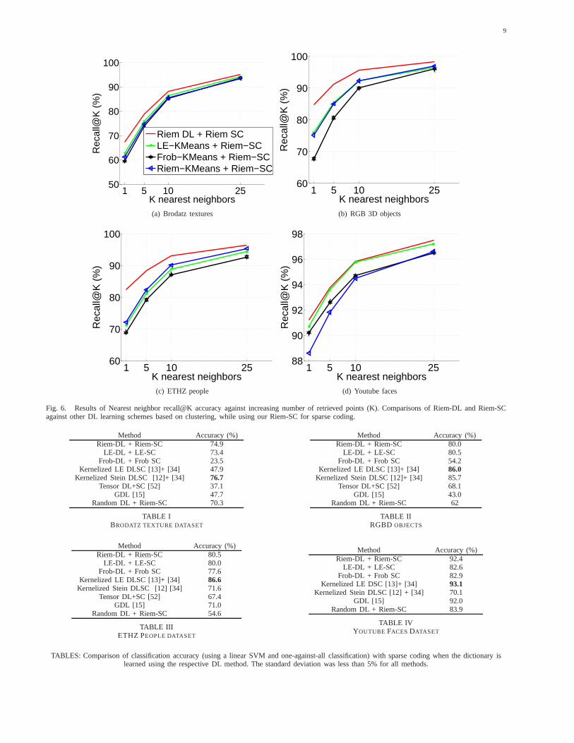
Fig. 6. Results of Nearest neighbor recall@K accuracy against increasing number of retrieved points (K). Comparisons of Riem-DL and Riem-SCagainst other DL learning schemes based on clustering, while using our Riem-SC for sparse coding.

Method Accuracy (%)Riem-DL + Riem-SC 74.9

LE-DL + LE-SC 73.4Frob-DL + Frob SC 23.5

Kernelized LE DLSC [13]+ [34] 47.9Kernelized Stein DLSC [12]+ [34] 76.7

Tensor DL+SC [52] 37.1GDL [15] 47.7

Random DL + Riem-SC 70.3

TABLE IBRODATZ TEXTURE DATASET

Method Accuracy (%)Riem-DL + Riem-SC 80.0

LE-DL + LE-SC 80.5Frob-DL + Frob SC 54.2

Kernelized LE DLSC [13]+ [34] 86.0Kernelized Stein DLSC [12]+ [34] 85.7

Tensor DL+SC [52] 68.1GDL [15] 43.0

Random DL + Riem-SC 62

TABLE IIRGBD OBJECTS

Method Accuracy (%)Riem-DL + Riem-SC 80.5

LE-DL + LE-SC 80.0Frob-DL + Frob SC 77.6

Kernelized LE DLSC [13]+ [34] 86.6Kernelized Stein DLSC [12] [34] 71.6

Tensor DL+SC [52] 67.4GDL [15] 71.0

Random DL + Riem-SC 54.6

TABLE IIIETHZ PEOPLE DATASET

Method Accuracy (%)Riem-DL + Riem-SC 92.4

LE-DL + LE-SC 82.6Frob-DL + Frob SC 82.9

Kernelized LE DSC [13]+ [34] 93.1Kernelized Stein DLSC [12] + [34] 70.1

GDL [15] 92.0Random DL + Riem-SC 83.9

TABLE IVYOUTUBE FACES DATASET

TABLES: Comparison of classification accuracy (using a linear SVM and one-against-all classification) with sparse coding when the dictionary islearned using the respective DL method. The standard deviation was less than 5% for all methods.

10

0 20 40 600

100

200

300

400

iteration

obje

ctiv

e

dim=3dim=5dim=10dim=20

Fig. 5. Dictionary Learning objective using Riemannian conjugategradient descent against increasing number of iterations (alternating withthe sparse coding sub-problem). We plot the convergence of the objectivefor various dimensionality of the data matrices.

every frame, the object was segmented out and 18 dimen-sional feature vectors generated for every 3D point in thecloud (and thus18×18 covariance descriptors); the featureswe used are as follows:

FRGBD = [x, y, z, Ir, Ig, Ib, Ix, Iy, Ixx, Iyy, Ixy,

Im, δx, δy, δm, νx, νy, νz] , (23)

where the first three dimensions are the spatial coordinates,Im is the magnitude of the intensity gradient,δ’s representgradients over the depth-maps, andν represents the surfacenormal at the given 3D point.

4) Youtube Faces Dataset:In this experiment, we eval-uate the performance of the Riemannian DLSC setup todeal with a larger dataset of high-dimensional covariancedescriptors for face recognition. To this end, we used thechallenging Youtube faces dataset [48] that consists of 3425short video clips of 1595 individuals, each clip containingbetween 48–6K frames. There are significant variations inhead pose, context, etc. for each person across clips andour goal is to associate a face with its ground truth personlabel. We proceed by first cropping out face regions fromthe frames by applying a state-of-the-art face detector [54],which results in approximately 196K face instances. Asmost of the faces within a clip do not have significantvariations, we subsample this set randomly to generate ourdataset of∼43K face patches. Next, we convolved theimage with a filter bank of 40 Gabor filters with 5 scalesand 8 different orientations to extract the facial featuresforeach pixel, generating40× 40 covariances.

D. Experimental Setup

1) Evaluation Techniques:We evaluated our algorithmsfrom two perspectives, namely (i) nearest neighbor (NN)retrieval against a gallery set via computing the Euclideandistances between sparse codes, and (ii) one-against-allclassification using a linear SVM trained over the sparsecodes. Given that computing the geodesic distance betweenSPD matrices is expensive, while the Frobenius distancebetween them results in poor accuracy, the goal of the firstexperiment is to evaluate the quality of sparse coding to

approximate the input data in terms of codes that belongto the non-negative orthant of the Euclidean space – su-perior performance implying that the sparse codes provideefficient representations that could bypass the Riemanniangeometry, and can enable other faster indexing schemessuch as locality sensitive hashing for faster retrieval. Oursecond experiment evaluates the linearity of the space ofsparse codes – note that they are much higher dimensionalthan the original covariances themselves and thus we expectthem to be linearly separable in the sparse space.

2) Evaluation Metric: For classification experiments,we use the one-against-all classification accuracy as theevaluation metric. For NN retrieval experiments, we usethe Recall@K accuracy, which is defined as follows. Givena galleryX and a query setQ. Recall@K computes theaverage accuracy when retrievingK nearest neighbors fromX for each instance inQ. SupposeGq

K stands for the setof ground truth class labels associated with theqth query,and if Sq

K denotes the set of labels associated with theKneighbors found by some algorithm for theq queries, then

Recall@K =1

|Q|

∑

q∈Q

|GqK ∩ Sq

K |

|GqK |

. (24)

3) Data Split: All the experiments used 5-fold cross-validation in which 80% of the datasets were used fortraining the dictionary,10% for generating the gallery setor as training set for the linear SVM, and the rest as thetest/query points. We evaluate three setups for generatingthe dictionaries, (i) using a proper dictionary learning strat-egy, and (ii) using clustering the training set via K-Meansusing the appropriate distance metric, and (iii) randomsampling of the training set.

4) Hyperparameters:The size of the dictionary wasconsidered to be twice the number of classes in therespective dataset. This scheme was considered for allthe comparison methods as well. We experimented withlarger sizes, but found that performance generally almostsaturates. This is perhaps because the datasets that we usealready have a large number of classes, and thus the dictio-nary sizes generated using this heuristic makes them alreadysignificantly overcomplete. The other hyperparameter in oursetup is the sparsity of the generated codes. As the differentsparse coding methods (including ours and the methods thatwe compare to) have varied sensitivity to the regularizationparameter, comparing all the methods to different sparsitiesturned out to be cumbersome. Thus, we decided to fixthe sparsity of all methods to 10%-sparse and adjusted theregularization parameter for each method appropriately (ona small validation set separate from the training set). Tothis end, we usedλB = 0.1 for textures,10 for the ETHZand RGBD datasets, and 100 for the faces dataset. For thefaces dataset, we found it to be difficult to attain the desiredsparsity by tuning the regularization parameter. Thus, weused a regularization of 100 and selected the top 10% sparsecoefficients.

5) Implementation Details:Our DLSC scheme was im-plemented in MATLAB. We used the ManOpt Riemanniangeometric optimization toolbox [55] for implementing the

11

1 5 10 2520

40

60

80

100

K nearest neighbors

Rec

all@

K (

%)

LEFrobKernelized Stein, Harandi−2012Random DL + Riem−SCKernelized Stein, Harandi−2015Kernelized LE, Li−2013GDL, Sra&Cherian−2012TSC, Sivalingam−2010Riemannian (this paper)

(a) Brodatz textures

1 5 10 2540

50

60

70

80

90

100

K nearest neighbors

Rec

all@

K (

%)

(b) RGB 3D objects

1 5 10 2560

70

80

90

100

K nearest neighbors

Rec

all@

K (

%)

(c) ETHZ people

1 5 10 2550

60

70

80

90

100

K nearest neighbors

Rec

all@

K (

%)

(d) Youtube faces

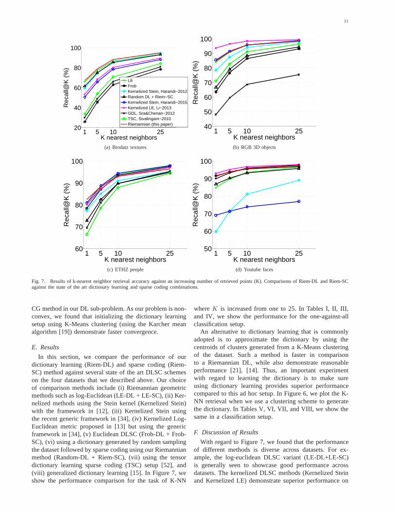
Fig. 7. Results of k-nearest neighbor retrieval accuracy against an increasing number of retrieved points (K). Comparisons of Riem-DL and Riem-SCagainst the state of the art dictionary learning and sparse coding combinations.

CG method in our DL sub-problem. As our problem is non-convex, we found that initializing the dictionary learningsetup using K-Means clustering (using the Karcher meanalgorithm [19]) demonstrate faster convergence.

E. Results

In this section, we compare the performance of ourdictionary learning (Riem-DL) and sparse coding (Riem-SC) method against several state of the art DLSC schemeson the four datasets that we described above. Our choiceof comparison methods include (i) Riemannian geometricmethods such as log-Euclidean (LE-DL + LE-SC), (ii) Ker-nelized methods using the Stein kernel (Kernelized Stein)with the framework in [12], (iii) Kernelized Stein usingthe recent generic framework in [34], (iv) Kernelized Log-Euclidean metric proposed in [13] but using the genericframework in [34], (v) Euclidean DLSC (Frob-DL + Frob-SC), (vi) using a dictionary generated by random samplingthe dataset followed by sparse coding using our Riemannianmethod (Random-DL + Riem-SC), (vii) using the tensordictionary learning sparse coding (TSC) setup [52], and(viii) generalized dictionary learning [15]. In Figure 7, weshow the performance comparison for the task of K-NN

whereK is increased from one to 25. In Tables I, II, III,and IV, we show the performance for the one-against-allclassification setup.

An alternative to dictionary learning that is commonlyadopted is to approximate the dictionary by using thecentroids of clusters generated from a K-Means clusteringof the dataset. Such a method is faster in comparisonto a Riemannian DL, while also demonstrate reasonableperformance [21], [14]. Thus, an important experimentwith regard to learning the dictionary is to make sureusing dictionary learning provides superior performancecompared to this ad hoc setup. In Figure 6, we plot the K-NN retrieval when we use a clustering scheme to generatethe dictionary. In Tables V, VI, VII, and VIII, we show thesame in a classification setup.

F. Discussion of Results

With regard to Figure 7, we found that the performanceof different methods is diverse across datasets. For ex-ample, the log-euclidean DLSC variant (LE-DL+LE-SC)is generally seen to showcase good performance acrossdatasets. The kernelized DLSC methods (Kernelized Steinand Kernelized LE) demonstrate superior performance on

12

Method Accuracy (%)Riem-DL + Riem-SC 74.9

LE-KMeans + Riem-SC 70.0Frob-KMeans + Riem-SC 66.5Riem-KMeans +Riem-SC 70.0

TABLE VBRODATZ TEXTURE DATASET

Method Accuracy (%)Riem-DL + Riem-SC 80.0

LE-KMeans + Riem-SC 66.2Frob-KMeans + Riem-SC 61.1Riem-KMeans +Riem-SC 67.8

TABLE VIRGBD OBJECTS

Method Accuracy (%)Riem-DL + Riem-SC 80.5

LE-KMeans + Riem-SC 54.9Frob-KMeans + Riem-SC 55.5Riem-KMeans +Riem-SC 57.5

TABLE VIIETHZ PEOPLE DATASET

Method Accuracy (%)Riem-DL + Riem-SC 92.4

LE-KMeans + Riem-SC 87.1Frob-KMeans + Riem-SC 88.7Riem-KMeans +Riem-SC 85.8

TABLE VIIIYOUTUBE FACES DATASET

TABLES: Comparison of classification accuracy (using a linear SVM and one-against-all classification) using Riemannian sparse coding (Riem-SC)while the dictionary atoms are taken as the centroids of K-Means clusters. The standard deviation was less than 8% for allmethods.

almost all the datasets. The most surprising of the resultsthat we found was for the Frob-DL case. It is gener-ally assumed that using Frobenius distance for comparingSPD matrices leads to poor accuracy, which we see inFigures 7(a), 7(b), and 7(c). However, for the Youtubefaces dataset, we found that the SPD matrices are poorlyconditioned. As a result, taking the logarithm (as in theLE-DL scheme) of these matrices results in amplifying theinfluence of the smaller eigenvalues, which is essentiallynoise. When learning a dictionary, the atoms will be learnedto reconstruct this noise against the signal, thus leading toinferior accuracy than for FrobDL or GDL which do not usematrix logarithm. We tried to circumvent this problem bytuning the small regularization that we add to the diagonalentries of these matrices, but that did not help. Other olderDLSC methods such as TSC are seen to be less accuratecompared to recent methods. We could not run the TSCmethod on the faces dataset as it was found to be tooslow to sparse code the larger covariances. In comparisonto all the above methods, Riem-DL+Riem-SC was foundto produce consistent, competitive (and sometimes better)performance, substantiating the usefulness of our proposedmethod. While running the experiments, we found thatthe initialization of our DL sub-problem (from K-Means)played an important role in achieving this superior per-formance. In Tables I, II, III, and IV we show the resultsfor classification using the sparse codes. The kernelized LEseems to be significantly better in this setting. However, ourRiemannian scheme does demonstrate promise by being thesecond best in most of the datasets.

The usefulness of our Riem-DL is further evaluatedagainst alternative DL schemes via clustering in Figure 6.We see that learning the dictionary using Riem-DL demon-strates the best performance against the next best andefficient alternative of using the LE-KMeans that was donein [21]. Using Frob-KMeans or using a random dictionaryare generally seen to have inferior performance comparedto other learning methods. In Tables V, VI, VII, and VIII,a similar trend is seen in the classification setting.

VI. CONCLUSIONS

In this paper, we proposed a novel setup for dictionarylearning and sparse coding of data in the form of SPDmatrices. In contrast to prior methods that use proxysimilarity distance measures to define the sparse codingapproximation loss, our formulation used a loss driven bythe natural Riemannian metric (affine invariant Riemannianmetric) on the SPD manifold. We proposed an efficientadaptation of the well-known non-linear conjugate gradientmethod for learning the dictionary in the product space ofSPD manifolds and a fast algorithm for sparse coding basedon the spectral projected gradient. Our experiments onsimulated and several benchmark computer vision datasetsdemonstrated the superior performance of our methodagainst prior works; especially our results showed thatlearning the dictionary using our scheme leads to signif-icantly better accuracy (in retrieval and classification) thanother heuristic and approximate schemes to generate thedictionary.

APPENDIX

Here we prove Theorem 3.

Lemma 4. Let Z ∈ GL(d) and let X ∈ Sd+. Then,ZTXZ ∈ Sd+.

Lemma 5. The Frechet derivative [56, see e.g., Ch. 1] ofthe mapX 7→ logX at a point Z in the directionE isgiven by

D log(Z)(E) =∫

1

0(βZ + (1− β)I)−1E(βZ + (1− β)I)−1dβ.

(25)

Proof: See e.g., [56, Ch. 11].

Corollary 6. Consider the mapℓ(α) := α ∈ Rn+ 7→

Tr(log(SM(α)S)H), whereM is a map fromRn+ → S

d+

andH ∈ Sd, S ∈ Sd+. Then, for1 ≤ p ≤ n, we have

∂ℓ(α)∂αp

=∫ 1

0 Tr[KβS∂M(α)∂αp

SKβH ]dβ,

whereKβ := (βSM(α)S + (1− β)I)−1.

13

Proof: Simply apply the chain-rule of calculus and uselinearity of Tr(·).

Lemma 7. The Frechet derivative of the mapX 7→ X−1

at a pointZ in directionE is given by

D(Z−1)(E) = −Z−1EZ−1. (26)

We are now ready to prove Theorem 3.Thm. 3: We show that the Hessian∇2φ(α) 0 on

A. To ease presentation, we writeS = X−1/2, M ≡M(α) =

∑

i αiBi, and let Dq denote the differentialoperatorDαq

. Applying this operator to the first-derivativegiven by Lemma 2 (in Section IV-B), we obtain (using theproduct rule) the sum

Tr(

[Dq log(SMS)](SMS)−1SBpS)

+Tr(

log(SMS)Dq[(SMS)−1SBpS])

.

We now treat these two terms individually. To the first weapply Corr. 6. So

Tr(

[Dq log(SMS)](SMS)−1SBpS)

=∫ 1

0Tr(KβSBqSKβ(SMS)−1SBpS)dβ

=∫ 1

0 Tr(SBqSKβ(SMS)−1SBpSKβ·)dβ

=∫ 1

0〈Ψβ(p), Ψβ(q)〉M dβ,

where the inner-product〈·, ·〉M is weighted by(SMS)−1

and the mapΨβ(p) := SBpSKβ. We find a similar inner-product representation for the second term too. Startingwith Lemma 7 and simplifying, we obtain

Tr(

log(SMS)Dq[(SMS)−1SBpS])

= −Tr(

log(SMS)(SMS)−1SBqM−1BpS

)

= Tr(

−S log(SMS)S−1M−1BqM−1Bp

)

= Tr(

M−1Bp[−S log(SMS)S−1]M−1Bq

)

.

By assumption∑

i αiBi = M X , which impliesSMS I. Since log(·) is operator monotone [26], itfollows that log(SMS) 0; an application of Lemma 4then yieldsS log(SMS)S−1 0. Thus, we obtain theweighted inner-product

Tr(

M−1Bp[−S log(SMS)S−1]M−1Bq

)

=⟨

M−1Bp, M−1Bq

⟩

L,

whereL = [−S log(SMS)S−1] 0, whereby〈·, ·〉L is avalid inner-product.

Thus, the second partial derivatives ofφ may be ulti-mately written as

∂2φ(α)

∂αp∂αq= 〈Γ(Bq), Γ(Bp)〉 ,

for some mapΓ and some corresponding inner-product(the map and the inner-product are defined by our analysisabove). Thus, we have established that the Hessian is aGram matrix, which shows it is semidefinite. Moreover, iftheBi are different (1 ≤ i ≤ n), then the Hessian is strictlypositive definite.

REFERENCES

[1] O. Tuzel, F. Porikli, and P. Meer., “Region Covariance: AFastDescriptor for Detection and Classification,” inECCV, 2006.

[2] S. Jayasumana, R. Hartley, M. Salzmann, H. Li, and M. Ha-randi, “Kernel methods on riemannian manifolds with gaussianrbf kernels,” IEEE Transactions on Pattern Analysis and MachineIntelligence, 2015.

[3] F. Porikli, and O. Tuzel, “Covariance tracker,”Computer Vision andPattern Recognition, June 2006.

[4] A. Cherian, V. Morellas, N. Papanikolopoulos, and S. J. Bedros,“Dirichlet process mixture models on symmetric positive definitematrices for appearance clustering in video surveillance applica-tions,” in Computer Vision and Pattern Recognition. IEEE, 2011.

[5] D. Fehr, A. Cherian, R. Sivalingam, S. Nickolay, V. Morellas,and N. Papanikolopoulos, “Compact covariance descriptorsin 3Dpoint clouds for object recognition,” inInternational conference onRobotics and Automation. IEEE, 2012.

[6] B. Ma, Y. Wu, and F. Sun, “Affine object tracking using kernel-basedregion covariance descriptors,” inFoundations of Intelligent Systems.Springer, 2012, pp. 613–623.

[7] J. Mairal, F. Bach, and J. Ponce, “Sparse modeling for image andvision processing,”Foundations and Trends in Computer Graphicsand Vision, vol. 8, no. 2, pp. 85–283, 2014.

[8] T. Guha and R. K. Ward, “Learning sparse representationsfor humanaction recognition,” IEEE Transactions on Pattern Analysis andMachine Intelligence, vol. 34, no. 8, pp. 1576–1588, 2012.

[9] J. Wright, A. Y. Yang, A. Ganesh, S. S. Sastry, and Y. Ma, “Robustface recognition via sparse representation,”IEEE Transactions onPattern Analysis and Machine Intelligence, vol. 31, no. 2, pp. 210–227, 2009.

[10] A. Cherian, “Nearest neighbors using compact sparse codes,” inInternational Conference on Machine Learning, 2014.

[11] M. Harandi, C. Sanderson, C. Shen, and B. C. Lovell, “Dictionarylearning and sparse coding on grassmann manifolds: An extrinsicsolution,” in International Conference on Computer Vision. IEEE,2013.

[12] M. T. Harandi, C. Sanderson, R. Hartley, and B. C. Lovell, “Sparsecoding and dictionary learning for symmetric positive definite ma-trices: A kernel approach,” inEuropean Conference on ComputerVision. Springer, 2012.

[13] P. Li, Q. Wang, W. Zuo, and L. Zhang, “Log-euclidean kernels forsparse representation and dictionary learning,” inICCV. IEEE,2013.

[14] R. Sivalingam, D. Boley, V. Morellas, and N. Papanikolopoulos,“Tensor sparse coding for region covariances,” inECCV. Springer,2010.

[15] S. Sra and A. Cherian, “Generalized dictionary learning for sym-metric positive definite matrices with application to nearest neighborretrieval,” in European Conference on Machine Learning. Springer,2011.

[16] V. Arsigny, P. Fillard, X. Pennec, and N. Ayache, “Log-Euclideanmetrics for fast and simple calculus on diffusion tensors,”MagneticResonance in Medicine, vol. 56, no. 2, pp. 411–421, 2006.

[17] S. Sra, “Positive definite matrices and the S-divergence,” arXivpreprint arXiv:1110.1773, 2011.

[18] M. Moakher and P. G. Batchelor, “Symmetric positive-definitematrices: From geometry to applications and visualization,” in Vi-sualization and Processing of Tensor Fields. Springer, 2006, pp.285–298.

[19] X. Pennec, P. Fillard, and N. Ayache, “A Riemannian frameworkfor tensor computing,”International Journal of Computer Vision,vol. 66, no. 1, pp. 41–66, 2006.

[20] O. S. Rothaus, “Domains of positivity,” inAbhandlungen aus demMathematischen Seminar der Universitat Hamburg, vol. 24, no. 1.Springer, 1960, pp. 189–235.

[21] A. Cherian and S. Sra, “Riemannian sparse coding for positivedefinite matrices,” inEuropean Conference on Computer Vision.Springer, 2014.

[22] P.-A. Absil, R. Mahony, and R. Sepulchre,Optimization algorithmson matrix manifolds. Princeton University Press, 2009.

[23] G. Cheng and B. C. Vemuri, “A novel dynamic system in the space ofspd matrices with applications to appearance tracking,”SIAM journalon imaging sciences, vol. 6, no. 1, pp. 592–615, 2013.

[24] Y. E. Nesterov and M. J. Todd, “On the Riemannian geometrydefined by self-concordant barriers and interior-point methods,”

14

Foundations of Computational Mathematics, vol. 2, no. 4, pp. 333–361, 2002.

[25] S. Lang,Fundamentals of differential geometry. Springer Science& Business Media, 2012, vol. 191.

[26] R. Bhatia,Positive Definite Matrices. Princeton University Press,2007.

[27] M. Aharon, M. Elad, and A. Bruckstein, “K-SVD: An algorithm fordesigning overcomplete dictionaries for sparse representation,” IEEETransactions on Signal Processing, vol. 54, no. 11, pp. 4311–4322,2006.

[28] M. Elad and M. Aharon, “Image denoising via learned dictionariesand sparse representation,” inComputer Vision and Pattern Recog-nition, 2006.

[29] R. Sivalingam, D. Boley, V. Morellas, and N. Papanikolopoulos,“Positive definite dictionary learning for region covariances,” inInternational Conference on Computer Vision. IEEE, 2011.

[30] K. Guo, P. Ishwar, and J. Konrad, “Action recognition using sparserepresentation on covariance manifolds of optical flow,” inInterna-tional Conference on Advanced Video and Signal based Surveillance.IEEE, 2010.

[31] J. Ho, Y. Xie, and B. Vemuri, “On a nonlinear generalization ofsparse coding and dictionary learning,” inInternational Conferenceon Machine Learning, 2013.

[32] A. Cichocki, S. Cruces, and S.-i. Amari, “Log-determinant di-vergences revisited: Alpha-beta and gamma log-det divergences,”Entropy, vol. 17, no. 5, pp. 2988–3034, 2015.

[33] A. Cherian, S. Sra, A. Banerjee, and N. Papanikolopoulos, “Jensen-bregman logdet divergence with application to efficient similaritysearch for covariance matrices,”IEEE Transactions on PatternAnalysis and Machine Intelligence, vol. 35, no. 9, pp. 2161–2174,2013.

[34] M. Harandi and M. Salzmann, “Riemannian coding and dictionarylearning: Kernels to the rescue,”Computer Vision and PatternRecognition, 2015.

[35] A. Feragen, F. Lauze, and S. Hauberg, “Geodesic exponentialkernels: When curvature and linearity conflict,”arXiv preprintarXiv:1411.0296, 2014.

[36] X. Pennec, R. Stefanescu, V. Arsigny, P. Fillard, and N.Ayache,“Riemannian elasticity: A statistical regularization framework fornon-linear registration,” inInternational Conference on MedicalImage Computing and Computer Assisted Interventions. Springer,2005.

[37] P.-A. Absil, C. G. Baker, and K. A. Gallivan, “Trust-region methodson riemannian manifolds,”Foundations of Computational Mathemat-ics, vol. 7, no. 3, pp. 303–330, 2007.

[38] D. P. Bertsekas and D. P. Bertsekas,Nonlinear Programming, 2nd ed.Athena Scientific, 1999.

[39] J.-B. Hiriart-Urruty and C. Lemarechal,Fundamentals of convexanalysis. Springer, 2001.

[40] J. Barzilai and J. M. Borwein, “Two-Point Step Size GradientMethods,” IMA J. Num. Analy., vol. 8, no. 1, 1988.

[41] M. Schmidt, E. van den Berg, M. Friedlander, and K. Murphy,“Optimizing Costly Functions with Simple Constraints: A Limited-Memory Projected Quasi-Newton Algorithm,” inInternational Con-ference on Artificial Intelligence and Statistics, 2009.

[42] E. G. Birgin, J. M. Martınez, and M. Raydan, “Algorithm813: SPG -Software for Convex-constrained Optimization,”ACM Transactionson Mathematical Software, vol. 27, pp. 340–349, 2001.

[43] Y. Pang, Y. Yuan, and X. Li, “Gabor-based region covariancematrices for face recognition,”IEEE Transactions on Circuits andSystems for Video Technology, vol. 18, no. 7, pp. 989–993, 2008.

[44] M. T. Harandi, M. Salzmann, and R. Hartley, “From manifold tomanifold: Geometry-aware dimensionality reduction for spd matri-ces,” inEuropean Conference on Computer Vision. Springer, 2014.

[45] K. Lai, L. Bo, X. Ren, and D. Fox, “A large-scale hierarchicalmulti-view RGB-D object dataset,” inInternational Conference onRobotics and Automation, 2011.

[46] T. Ojala, M. Pietikainen, and D. Harwood, “A comparative study oftexture measures with classification based on featured distributions,”Pattern recognition, vol. 29, no. 1, pp. 51–59, 1996.

[47] A. Ess, B. Leibe, and L. V. Gool, “Depth and appearance for mobilescene analysis,” inInternational Conference on Computer Vision.IEEE, 2007.

[48] T. H. Lior Wolf and I. Maoz, “Face recognition in unconstrainedvideos with matched background similarity,” inComputer Vision andPattern Recognition. IEEE, 2011.

[49] R. Luis-Garcıa, R. Deriche, and C. Alberola-Lopez, “Texture andcolor segmentation based on the combined use of the structure tensorand the image components,”Signal Processing, vol. 88, no. 4, pp.776–795, 2008.

[50] B. Ma, Y. Su, F. Jurieet al., “Bicov: a novel image representationfor person re-identification and face verification,” inBMVC, 2012.

[51] W. Schwartz and L. Davis, “Learning Discriminative Appearance-Based Models Using Partial Least Squares,” inProceedings ofthe XXII Brazilian Symposium on Computer Graphics and ImageProcessing, 2009.

[52] R. Sivalingam, D. Boley, V. Morellas, and N. Papanikolopoulos,“Tensor dictionary learning for positive definite matrices,” IEEETransactions on Image Processing, vol. 24, no. 11, pp. 4592–4601,2015.

[53] D. A. Fehr, Covariance based point cloud descriptors for objectdetection and classification. University Of Minnesota, 2013.

[54] X. Zhu and D. Ramanan, “Face detection, pose estimation, andlandmark localization in the wild,” inComputer Vision and PatternRecognition. IEEE, 2012.

[55] N. Boumal, B. Mishra, P.-A. Absil, and R. Sepulchre, “Manopt,a matlab toolbox for optimization on manifolds,”The Journal ofMachine Learning Research, vol. 15, no. 1, pp. 1455–1459, 2014.

[56] N. Higham, Functions of Matrices: Theory and Computation.SIAM, 2008.