Final Report

Parallel Implementation of Sparse Coding and Dictionary Learning on GPU

Huynh Manh Parallel Distributed System, CSCI 7551

Fall 2016

1. Introduction While the goal of sparse coding is to find the sparse representation of a set of input signals given a learned dictionary, the goal of K-SVD is to create a set of compact and meaningful atoms that is better represent the input data by repeating the steps of finding sparse coding and tuning dictionary atoms. A sparse coding involves finding the "best matching" projections of multidimensional data onto the span of an over-complete (i.e., redundant) dictionary D. Through sparse coding process, a given input signal can be described as the linear combination of the learned atoms. Dictionary D (size � � �) is said to be over-complete if K > N. The advantage of having an over-complete basis is that our basis vectors are better able to capture structures and patterns inherent in the input data. The aim of sparse coding is to find a set of basis vectors �� (atom) such that we can represent an input vector � as a linear combination of these basis vectors

� = � ����

�

�

The dictionary learning method becomes very useful in a wide range of applications since it is able to obtain a compact high-fidelity representation of the observed signal and uncover semantic information. Such a sparse representation, if computed correctly, might naturally encode semantic information about the image. These applications include image compression, image denoising, and recently be adapted to face recognition and human tracking.

The aim of dictionary learning again is to learn a dictionary � ∈ ��� �, where K is the number of atoms and � is the dimension of input signal. Given the input signal x, we want to find the sparse

vector � such that � ≈ ��, or �|� ��|� < � for some small value � and �� norm. The sparse

vector � contains the representation coefficient of atoms in D, or we can think of each of element in sparse representation � is the contribution of each of atoms to construct x. Normally, the norm �� is L1,L2, or L1. In this project, the L2 is used for its simplicity. The table 1 shows the notation we use in this project.

In this project, we aim to exploit fully parallel algorithm for sparse coding and dictionary learning for the purpose of multi-target tracking application. Specifically, dictionary is learned to classify the target's appearance, which is an important component and also highly computational in tracking. Since real-time tracking requires the processing time within the frame speed, we expect to speed-up the current serial algorithm to match this requirement. We note that the tracking algorithms may consist of many other components such as human detection, motion prediction, Hungarian algorithm, which also consume lots of computation. However, in the scope of this

project, we mainly focus on dictionary learning and leave the other parts as future works. In the next section, we will discuss more about the algorithm for sparse coding and dictionary learning.

2. Matching pursuit algorithm The objective function of sparse representation is minimize find the sparse vector � for each of input x that satisfy the equation: �� = �. However, since D is over-complete matrix, solving that undetermined equations resulting infinitely many solutions. Among those infinite solutions we expect to have the sparsest solution, which makes this solution is unique and also turns out to be a useful property for many applications. Thus, solving �� = � becomes an optimization problem of finding the minimum atoms that minimize the error.

min�|�|��

�. � �|�� �|��

�≤ �� (1)

Where �|�|��

is the L0 norm, which denotes the number of zero element in sparse vector. In

overall, the goal of sparse coding algorithm is to find the sparsest vector that satisfy the condition �� close to x. Solving the equation 1 is proven an NP-hard problem. There is several research try to relaxed the constraint by using L1 norm instead of L0. Others using greedy matching algorithm (algorithm 1), and that is the algorithm of our focus in this proposal. The idea of greedy matching algorithm is searching through all atoms in dictionary to find the best match in the input x, calculating the residual error, and continue to find another atom in dictionary to further reduce the error. The process is recursive until there is smaller the error threshold.

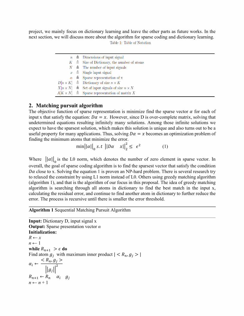
Algorithm 1 Sequential Matching Pursuit Algorithm

Input: Dictionary D, input signal x Output: Sparse presentation vector α Initialization: R ← x n ← 1 while ���� > � do Find atom �� with maximum inner product | < ��, �� > |

�� ← < ��, �� >

�������

���� ← �� �� �� n ← n + 1

end while end

2.1 Sequential implementation The following code is implementation of serial matching pursuit algorithm, which inputs are humanSet matrix [NxP] stores sets of P input features (RGB color histogram and spatial location of target) in feature dimension N, dictionary size [NxK]. Alpha matrix is set of sparse coding for each of feature input. DictionaryBuffer stores a list of input feature index that each of atom is used to calculate its sparse coding. For example, if DictionaryBuffer[1] = {1,3,4}, it means that atom 1 is used to calculate sparse coding for input feature 1, 3, 4. This DictionaryBuffer actually is not in the matching pursuit algorithm but it improves computation efficient even for serial code in update dictionary stage, this will be further explained in updating dictionary section. Another important element should be noted is isChoosen matrix [Kx1], which marks an atom as choosen,

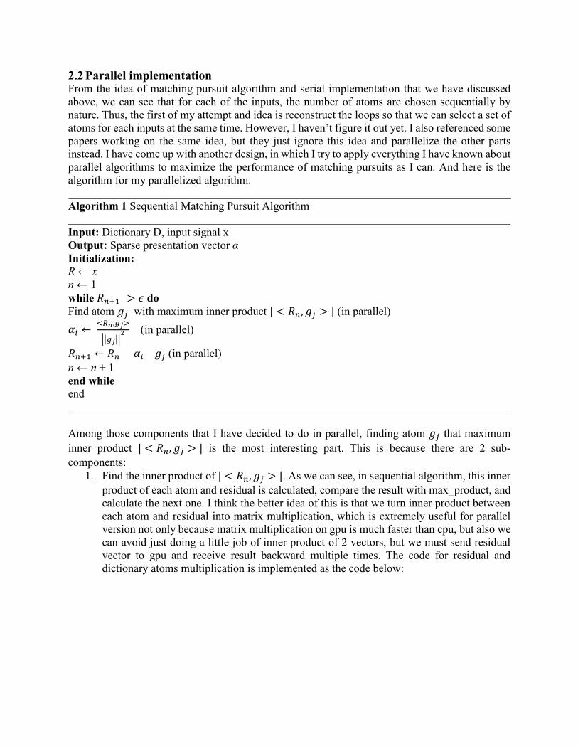
2.2 Parallel implementation From the idea of matching pursuit algorithm and serial implementation that we have discussed above, we can see that for each of the inputs, the number of atoms are chosen sequentially by nature. Thus, the first of my attempt and idea is reconstruct the loops so that we can select a set of atoms for each inputs at the same time. However, I haven’t figure it out yet. I also referenced some papers working on the same idea, but they just ignore this idea and parallelize the other parts instead. I have come up with another design, in which I try to apply everything I have known about parallel algorithms to maximize the performance of matching pursuits as I can. And here is the algorithm for my parallelized algorithm.

Algorithm 1 Sequential Matching Pursuit Algorithm

Input: Dictionary D, input signal x Output: Sparse presentation vector α Initialization: R ← x n ← 1 while ���� > � do Find atom �� with maximum inner product | < ��, �� > | (in parallel)

�� ← ���,���

������� (in parallel)

���� ← �� �� �� (in parallel) n ← n + 1 end while end

Among those components that I have decided to do in parallel, finding atom �� that maximum

inner product | < ��, �� > | is the most interesting part. This is because there are 2 sub-

components: 1. Find the inner product of | < ��, �� > |. As we can see, in sequential algorithm, this inner

product of each atom and residual is calculated, compare the result with max_product, and calculate the next one. I think the better idea of this is that we turn inner product between each atom and residual into matrix multiplication, which is extremely useful for parallel version not only because matrix multiplication on gpu is much faster than cpu, but also we can avoid just doing a little job of inner product of 2 vectors, but we must send residual vector to gpu and receive result backward multiple times. The code for residual and dictionary atoms multiplication is implemented as the code below:

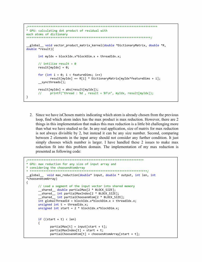
2. Since we have isChosen matrix indicating which atom is already chosen from the previous loop, find which atom index has the max product is max reduction. However, there are 2 things in this implementation that makes this max reduction is a little bit challenging more than what we have studied so far. In any real application, size of matrix for max reduction is not always divisible by 2, but instead it can be any size number. Second, comparing between 2 elements in the input array should not consider any further condition. It just simply chooses which number is larger. I have handled these 2 issues to make max reduction fit into this problem domain. The implementation of my max reduction is presented as following code:

/*************************************************************************** * GPU: calculating dot product of residual with each atoms of dictionary ************************************************************************/ __global__ void vector_product_matrix_kernel(double *DictionaryMatrix, double *R, double *result){ int myIdx = blockIdx.x*blockDim.x + threadIdx.x; // intilize result = 0 result[myIdx] = 0; for (int i = 0; i < featureDims; i++) result[myIdx] += R[i] * DictionaryMatrix[myIdx*featureDims + i]; __syncthreads(); result[myIdx] = abs(result[myIdx]); // printf("thread : %d , result = %f\n", myIdx, result[myIdx]); }

/******************************************************************* * GPU: max reduction for any size of input array and * considering the choosenAtomArray * ********************************************************************/ __global__ void max_reduction(double* input, double * output, int len, int *choosenAtomArray) { // Load a segment of the input vector into shared memory __shared__ double partialMax[2 * BLOCK_SIZE]; __shared__ int partialMaxIndex[2 * BLOCK_SIZE]; __shared__ int partialChoosenAtom[2 * BLOCK_SIZE]; int globalThreadId = blockIdx.x*blockDim.x + threadIdx.x; unsigned int t = threadIdx.x; unsigned int start = 2 * blockIdx.x*blockDim.x; if ((start + t) < len) { partialMax[t] = input[start + t]; partialMaxIndex[t] = start + t; partialChoosenAtom[t] = choosenAtomArray[start + t]; }

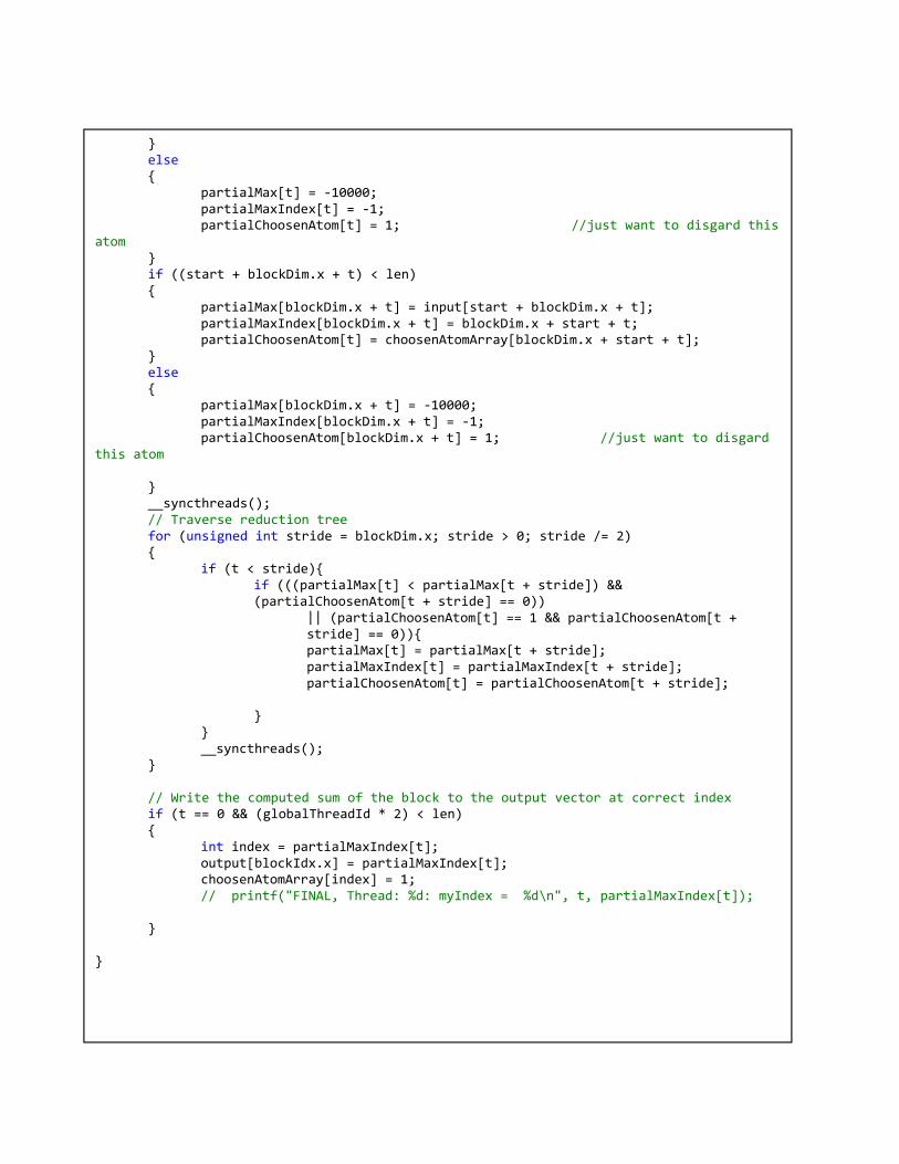
} else { partialMax[t] = -10000; partialMaxIndex[t] = -1; partialChoosenAtom[t] = 1; //just want to disgard this atom } if ((start + blockDim.x + t) < len) { partialMax[blockDim.x + t] = input[start + blockDim.x + t]; partialMaxIndex[blockDim.x + t] = blockDim.x + start + t; partialChoosenAtom[t] = choosenAtomArray[blockDim.x + start + t]; } else { partialMax[blockDim.x + t] = -10000; partialMaxIndex[blockDim.x + t] = -1; partialChoosenAtom[blockDim.x + t] = 1; //just want to disgard this atom } __syncthreads(); // Traverse reduction tree for (unsigned int stride = blockDim.x; stride > 0; stride /= 2) { if (t < stride){

if (((partialMax[t] < partialMax[t + stride]) && (partialChoosenAtom[t + stride] == 0))

|| (partialChoosenAtom[t] == 1 && partialChoosenAtom[t + stride] == 0)){

partialMax[t] = partialMax[t + stride]; partialMaxIndex[t] = partialMaxIndex[t + stride]; partialChoosenAtom[t] = partialChoosenAtom[t + stride]; } } __syncthreads(); } // Write the computed sum of the block to the output vector at correct index if (t == 0 && (globalThreadId * 2) < len) { int index = partialMaxIndex[t]; output[blockIdx.x] = partialMaxIndex[t]; choosenAtomArray[index] = 1; // printf("FINAL, Thread: %d: myIndex = %d\n", t, partialMaxIndex[t]); } }

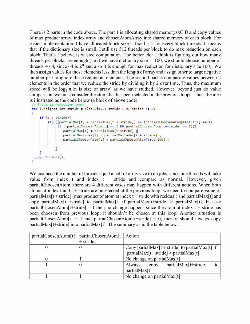
There is 2 parts in the code above. The part 1 is allocating shared memoryzxC B and copy values of max product array, index array and chosenAtomArray into shared memory of each block. For easier implementation, I have allocated block size is fixed 512 for every block threads. It means that if the dictionary size is small, I still use 512 threads per block to do max reduction on each block. That’s I believe is wasted computation. The better idea I think is figuring out how many threads per blocks are enough (i.e if we have dictionary size = 100, we should choose number of threads = 64, since 64 is 2� and also it is enough for max reduction for dictionary size 100). We then assign values for those elements less than the length of array and assign other to large negative number just to ignore these redundant elements. The second part is comparing values between 2 elements in the order that we reduce the stride by dividing it by 2 over time. Thus, the maximum speed will be log� � (n is size of array) as we have studied. However, beyond just do value comparison, we must consider the atom that has been selected in the previous loops. Thus, the idea is illustrated as the code below (a block of above code):

We just need the number of threads equal a half of array size to do jobs, since one threads will take value from index t and index t + stride and compare as normal. However, given partialChoosenAtom, there are 4 different cases may happen with different actions. When both atoms at index t and t + stride are unselected at the previous loop, we need to compare value of partialMax[t + stride] (max product of atom at index t + stride with residual) and partialMax[t] and copy partialMax[t +stride] to partialMax[t] if partialMax[t+stride] > partialMax[t]. In case partialChosenAtom[t+stride] = 1 then no change happens since the atom at index t + stride has been choosen from previous loop, it shouldn’t be chosen at this loop. Another situation is partialChosenAtom[t] = 1 and partialChosenAtom[t+stride] = 0, then it should always copy partialMax[t+stride] into partialMax[t]. The summary as in the table below: partialChosenAtom[t] partialChosenAtom[t

+ stride] Action

0 0 Copy partialMax[t + stride] to partialMax[t] if partialMax[t +stride] > partialMax[t]

0 1 No change on partialMax[t] 1 0 Always copy partialMax[t+stride] to

partialMax[t] 1 1 No change on partialMax[t]

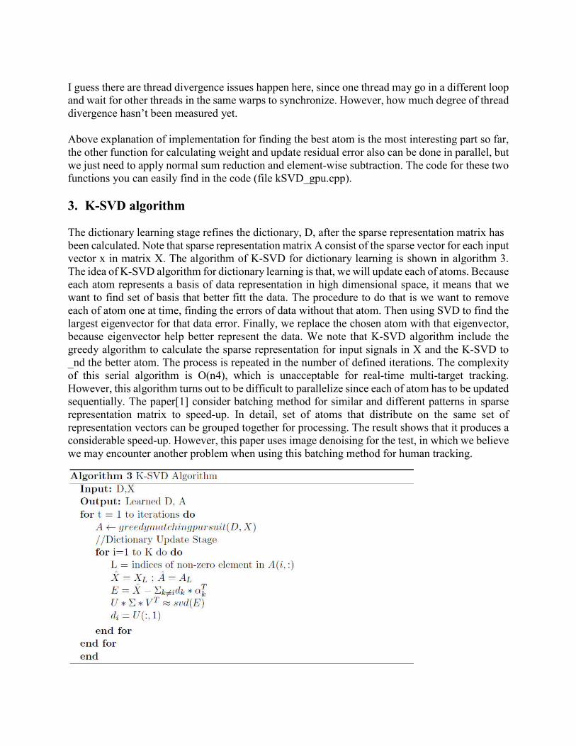
I guess there are thread divergence issues happen here, since one thread may go in a different loop and wait for other threads in the same warps to synchronize. However, how much degree of thread divergence hasn’t been measured yet. Above explanation of implementation for finding the best atom is the most interesting part so far, the other function for calculating weight and update residual error also can be done in parallel, but we just need to apply normal sum reduction and element-wise subtraction. The code for these two functions you can easily find in the code (file kSVD_gpu.cpp).

3. K-SVD algorithm

The dictionary learning stage refines the dictionary, D, after the sparse representation matrix has been calculated. Note that sparse representation matrix A consist of the sparse vector for each input vector x in matrix X. The algorithm of K-SVD for dictionary learning is shown in algorithm 3. The idea of K-SVD algorithm for dictionary learning is that, we will update each of atoms. Because each atom represents a basis of data representation in high dimensional space, it means that we want to find set of basis that better fitt the data. The procedure to do that is we want to remove each of atom one at time, finding the errors of data without that atom. Then using SVD to find the largest eigenvector for that data error. Finally, we replace the chosen atom with that eigenvector, because eigenvector help better represent the data. We note that K-SVD algorithm include the greedy algorithm to calculate the sparse representation for input signals in X and the K-SVD to _nd the better atom. The process is repeated in the number of defined iterations. The complexity of this serial algorithm is O(n4), which is unacceptable for real-time multi-target tracking. However, this algorithm turns out to be difficult to parallelize since each of atom has to be updated sequentially. The paper[1] consider batching method for similar and different patterns in sparse representation matrix to speed-up. In detail, set of atoms that distribute on the same set of representation vectors can be grouped together for processing. The result shows that it produces a considerable speed-up. However, this paper uses image denoising for the test, in which we believe we may encounter another problem when using this batching method for human tracking.

The idea of k-SVD is mainly based on Singular Value Decomposition, which is a linear algebra theorem saying that given any matrix, we always can factor this matrix into sets of orthonormal eigenvectors, an diagonal matrix and other sets of orthonormal vectors

And it is also proven that sets of orthonormal eigenvectors are principal components of X. The detailed of how principal component related to the eigenvector decomposition and singular value decomposition is in the presentation slides.

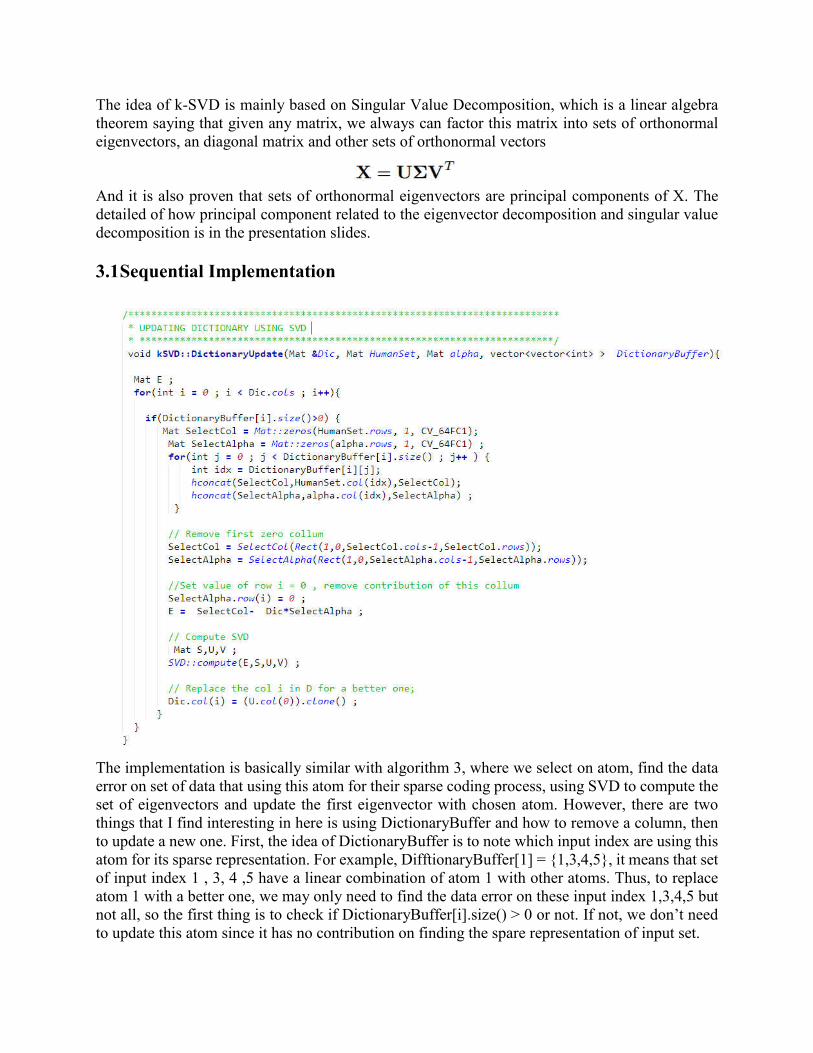
3.1 Sequential Implementation

The implementation is basically similar with algorithm 3, where we select on atom, find the data error on set of data that using this atom for their sparse coding process, using SVD to compute the set of eigenvectors and update the first eigenvector with chosen atom. However, there are two things that I find interesting in here is using DictionaryBuffer and how to remove a column, then to update a new one. First, the idea of DictionaryBuffer is to note which input index are using this atom for its sparse representation. For example, DifftionaryBuffer[1] = {1,3,4,5}, it means that set of input index 1 , 3, 4 ,5 have a linear combination of atom 1 with other atoms. Thus, to replace atom 1 with a better one, we may only need to find the data error on these input index 1,3,4,5 but not all, so the first thing is to check if DictionaryBuffer[i].size() > 0 or not. If not, we don’t need to update this atom since it has no contribution on finding the spare representation of input set.

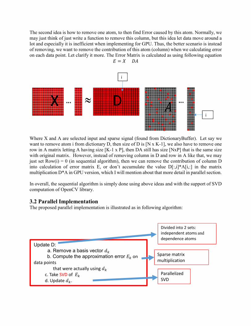
The second idea is how to remove one atom, to then find Error caused by this atom. Normally, we may just think of just write a function to remove this column, but this idea let data move around a lot and especially it is inefficient when implementing for GPU. Thus, the better scenario is instead of removing, we want to remove the contribution of this atom (column) when we calculating error on each data point. Let clarify it more. The Error Matrix is calculated as using following equation

� = � ��

Where X and A are selected input and sparse signal (found from DictionaryBuffer). Let say we want to remove atom i from dictionary D, then size of D is [N x K-1], we also have to remove one row in A matrix letting A having size [K-1 x P], then DA still has size [NxP] that is the same size with original matrix. However, instead of removing column in D and row in A like that, we may just set Row(i) = 0 (in sequential algorithm), then we can remove the contribution of column D into calculation of error matrix E, or don’t accumulate the value D[:,i]*A[i,:] in the matrix multiplication D*A in GPU version, which I will mention about that more detail in parallel section. In overall, the sequential algorithm is simply done using above ideas and with the support of SVD computation of OpenCV library.

3.2 Parallel Implementation The proposed parallel implementation is illustrated as in following algorithm:

i

i

Sparse matrix multiplication

Parallelized SVD

Update D: a. Remove a basis vector ��

b. Compute the approximation error �� on data points that were actually using ��

c. Take SVD of �� d. Update ��.

Divided into 2 sets: independent atoms and dependence atoms

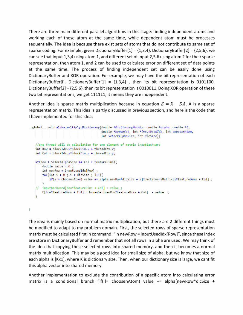
There are three main different parallel algorithms in this stage: finding independent atoms and

working each of these atom at the same time, while dependent atom must be processes

sequentially. The idea is because there exist sets of atoms that do not contribute to same set of

sparse coding. For example, given DictionaryBuffer[1] = {1,3,4}, DictionaryBuffer[2] = {2,5,6}, we

can see that input 1,3,4 using atom 1, and different set of input 2,5,6 using atom 2 for their sparse

representation, then atom 1, and 2 can be used to calculate error on different set of data points

at the same time. The process of finding independent set can be easily done using

DictionaryBuffer and XOR operation. For example, we may have the bit representation of each

DictionaryBuffer[i]. DictionaryBuffer[1] = {1,3,4} , then its bit representation is 0101100,

DictionaryBuffer[2] = {2,5,6}, then its bit representation is 0010011. Doing XOR operation of these

two bit representations, we get 111111, it means they are independent.

Another idea is sparse matrix multiplication because in equation � = � ��, A is a sparse

representation matrix. This idea is partly discussed in previous section, and here is the code that

I have implemented for this idea:

The idea is mainly based on normal matrix multiplication, but there are 2 different things must

be modified to adapt to my problem domain. First, the selected rows of sparse representation

matrix must be calculated first in command: “in newRow = inputUsedIdx[Row]”, since these index

are store in DictionaryBuffer and remember that not all rows in alpha are used. We may think of

the idea that copying these selected rows into shared memory, and then it becomes a normal

matrix multiplication. This may be a good idea for small size of alpha, but we know that size of

each alpha is [Kx1], where K is dictionary size. Then, when our dictionary size is large, we cant fit

this alpha vector into shared memory.

Another implementation to exclude the contribution of a specific atom into calculating error

matrix is a conditional branch “if(i!= choosenAtom) value += alpha[newRow*dicSize +

i]*DictionaryMatrix[i*featureDims + Col] “. This is a similar idea of removing an atom for

calculating error.

For parallel SVD algorithm, I haven’t done much research on this, but I know there are a lot of

different parallel methods for SVD.

4. Result

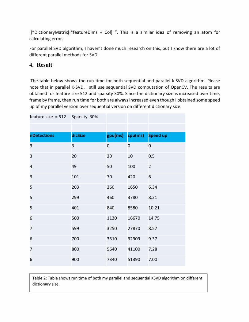
The table below shows the run time for both sequential and parallel k-SVD algorithm. Please

note that in parallel K-SVD, I still use sequential SVD computation of OpenCV. The results are

obtained for feature size 512 and sparsity 30%. Since the dictionary size is increased over time,

frame by frame, then run time for both are always increased even though I obtained some speed

up of my parallel version over sequential version on different dictionary size.

feature size = 512 Sparsity 30%

nDetections dicSize gpu(ms) cpu(ms) Speed up

3 3 0 0 0

3 20 20 10 0.5

4 49 50 100 2

3 101 70 420 6

5 203 260 1650 6.34

5 299 460 3780 8.21

5 401 840 8580 10.21

6 500 1130 16670 14.75

7 599 3250 27870 8.57

6 700 3510 32909 9.37

7 800 5640 41100 7.28

6 900 7340 51390 7.00

Table 2: Table shows run time of both my parallel and sequential KSVD algorithm on different

dictionary size.

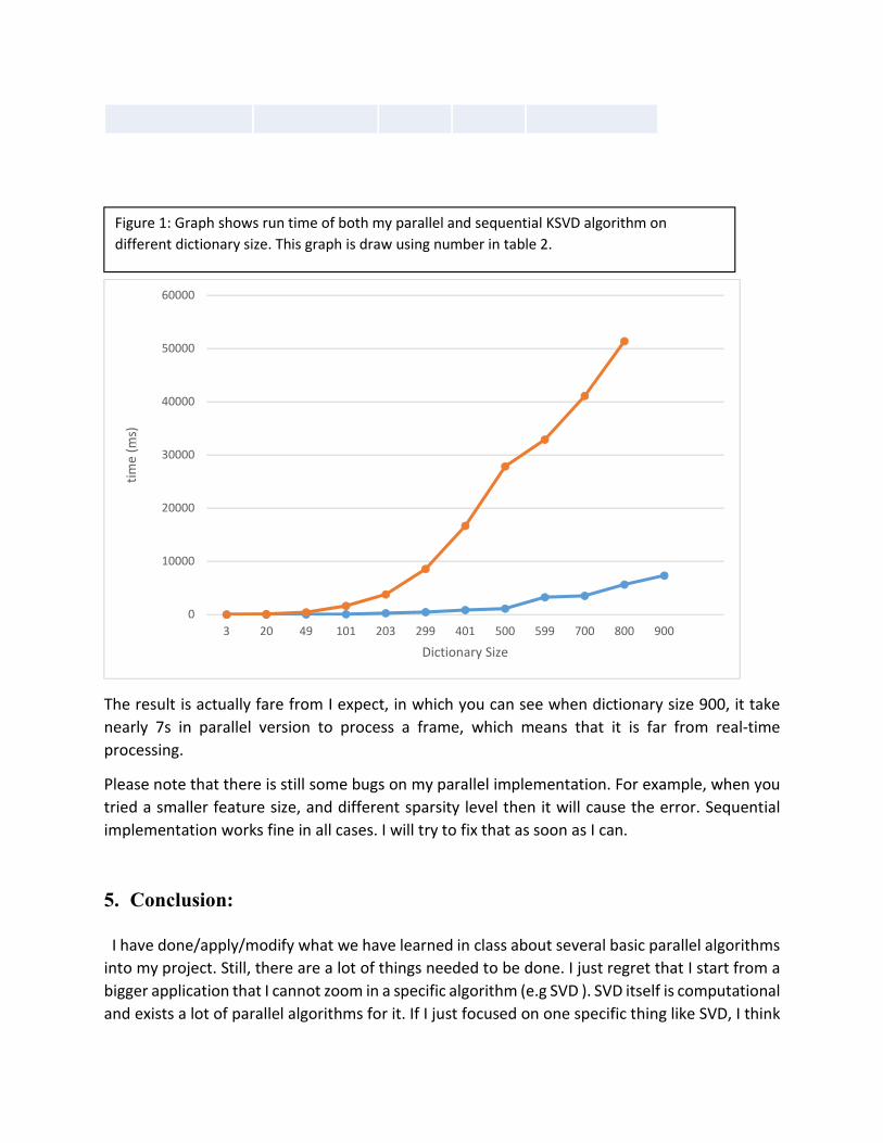
The result is actually fare from I expect, in which you can see when dictionary size 900, it take

nearly 7s in parallel version to process a frame, which means that it is far from real-time

processing.

Please note that there is still some bugs on my parallel implementation. For example, when you

tried a smaller feature size, and different sparsity level then it will cause the error. Sequential

implementation works fine in all cases. I will try to fix that as soon as I can.

5. Conclusion:

I have done/apply/modify what we have learned in class about several basic parallel algorithms

into my project. Still, there are a lot of things needed to be done. I just regret that I start from a

bigger application that I cannot zoom in a specific algorithm (e.g SVD ). SVD itself is computational

and exists a lot of parallel algorithms for it. If I just focused on one specific thing like SVD, I think

0

10000

20000

30000

40000

50000

60000

3 20 49 101 203 299 401 500 599 700 800 900

tim

e (m

s)

Dictionary Size

Figure 1: Graph shows run time of both my parallel and sequential KSVD algorithm on

different dictionary size. This graph is draw using number in table 2.

I can learn more about parallel algorithm. I do agree that what I am doing is broader, not much

parallel specific, even I have implemented some functions and not much presented them in class

since I spent too much time on explaining SVD and PCA, which are both new to me.

Another thing I am lacking is focusing on how lower level of hardware (GPUs) operates. It can be

how thread divergence in a warp affects on program, how to achieve and better bandwidth, how

much we can have better performance when using shared memory vs global memory and then

from that I may answer the question what is the best way to do in parallel.

Anyway, I found the course is useful and interesting for my research problem, which I can dive in

more, understand more and design an intelligent, high performance tracking system. The

tracking system is not just relied on dictionary learning, but it can be a parallel design in overall,

and it requires to think in parallel. Also, the pure computer vision problem need to be changed

to adapt to underlying hardware to be run efficiently. I hope that in the future, I can have a better

idea/ clearer idea and imagination, in which I still in vague right now, to have my best parallel

design for multi-target tracking. Again, if I have a chance to do this project again with time limited

time,I would like to pick just small specific algorithm like SVD to have chances learning more

about parallel algorithms.

****

All in all, thanks for your all recommendation/suggestions throughout this course. I hope to

receive any suggestions you may have by through emails or direct talking to me

References

[1] http://mathworld.wolfram.com/EigenDecompositionTheorem.html

[2] http://stattrek.com/matrix-algebra/covariance-matrix.aspx

[3] eigenvectors and SVD

https://www.cs.ubc.ca/~murphyk/Teaching/Stat406 Spring08/Lectures/linalg1.pdf

[4] https://www.cs.princeton.edu/picasso/mats/PCA-Tutorial-Intuition_jp.pdf

[5] Lu He, Timothy Miskell, Rui Liu, Hengyong Yu, Huijuan Xu, and Yan Luo. Scalable 2d k-svd parallel algorithm for dictionary learning on gpus. In Proceedings of the ACM International Conference on Computing Frontiers, pages 11{18. ACM, 2016.