Embed Size (px)
Citation preview

Research Collection
Doctoral Thesis
Redefining Plasmopara viticola epidemiological cycle bymolecular genetics
Author(s): Gobbin, Davide
Publication Date: 2003
Permanent Link: https://doi.org/10.3929/ethz-a-004709078
Rights / License: In Copyright - Non-Commercial Use Permitted
This page was generated automatically upon download from the ETH Zurich Research Collection. For moreinformation please consult the Terms of use.
ETH Library

Diss. ETH No. 15385
REDEFINING PLASMOPARA VITICOLA EPIDEMIOLOGICAL CYCLE
BY MOLECULAR GENETICS
A dissertation submitted to the
SWISS FEDERAL INSTITUTE OF TECHNOLOGY, ZÜRICH
for the degree of
DOCTOR OF NATURAL SCIENCES
Presented by
DAVIDE GOBBIN
Dipl. sc. Nat. ETHZ
born October 22th, 1973, citizen of Bidogno TI, Switzerland
Accepted on the recommendation of
Prof. Dr. Bruce McDonald, referent
Dr. Cesare Gessler, co-referent
Dr. Michel Clerjeau, co-referent
2004

DEDICA ET AL.
E qui si chiude non solamente un dottorato, ma anche un quinquennio di vita. Che dire? Ho
pagato il mio tributo alla scienza, computabile in un annetto di frustrazione (roba da tagliarsi
le vene) ma in cambio ho ottenuto quattro anni tra i più belli della mia vita. Non ho mai
viaggiato tanto (e così a scrocco) come in questo periodo. Ho iniziato col pupillo in Germania,
per poi recarmi a Geisenheim dal Bernd, a Oppenheim dal Georg, a Epernay dalla Marie-Laure
(che poi ha mollato l’osso), a Bordeaux dal Marc e soci e poi in Trentino, Veneto (cavolo, ho
mancato il Piemonte, sono uno stupido!) dall’Ilaria (ricordo con piacere le gite in rampichino
sulle Dolomiti… e le FUNIVIE soprattutto). Quando pensavo fosse tutto finito, ecco che la
Marina m’invita a Bologna e il Mauro nella leggendaria Cugnasco. Come poi dimenticare i
congressi? Quello in Portogallo è stato il più bello, abbiamo persino cantato in piedi sulle
sedie “se mi sum cioc menim a ca la biciclèta”, ma non da meno è stato quello a Napa (che
strage e che sbragoooo!) con annesse le visite ai parchi nazionali. E le escursioni
fitopatologiche? Abbiamo cavalcato il Trentino, la Grecia e la Romania. Abbiamo aperto gli
occhi su realtà che mai ci saremmo immaginati. Questi ultimi tre viaggi ci sono stati più utili
dal profilo umano che da quello scientifico. Devo aver dimenticato qualche posto in questa
lista, ma fa niente, tanto avete capito l’antifona. Dal profilo umano ho conosciuto persone
che ammiro (e invidio) per la loro determinazione e forza di carattere, come Cesare, Ilaria e
Mauro, che (in momenti di alcolemia) potrei addirittura acquisire come modelli di vita. A
parte gli scherzi, è bello avere frequentato persone tanto affidabili, schiette e oneste come
loro. Ma la persona che più mi ha seguito col cuore e con la mente è certamente una sola,
l’unica che un cervello esclusivista come il mio abbia saputo amare, apprezzare e stimare. E
dal canto suo, colei che cinque anni fa ha osato entare al Polyball dai sotterranei del Poly
sfidando correnti torride e polveri radioattive, lei mi ha dato tutto il sostegno che un uomo
possa desiderare. Rispetto, motivazione, incitamento, o forse, con una parola sola, amore.
Grazie cara Marianna, per tutto quello che mi hai dimostrato, per esserci sempre stata, per
avere respirato con me, per avermi abbracciato e mai più mollato nell’anno di frustrazione,
per avere scacciato con tanta forza le tentazioni disequilibranti del destino. Per avere
riconosciuto tanta forza in te, questo lavoro te lo dedico interamente. Se solo tu avessi lavato
i piatti un po’ più spesso, mi avresti reso davvero felice….

TABLE OF CONTENTS
Abstract 444
Riassunto 555
CHAPTER 1 666
General introduction
CHAPTER 2 113
Identification of microsatellite markers for Plasmopara viticola and establishment of high
throughput method for SSR analysis
CHAPTER 3 339
Genetic structure of a Plasmopara viticola population in an isolated Italian mountain
vineyard
CHAPTER 4 771
The importance of secondary inoculum of Plasmopara viticola to epidemics of grapevine
downy mildew
CHAPTER 5 109
A population genetic snapshot of Plasmopara viticola after 125 years of colonisation in
Europe
CHAPTER 6 137
General discussion
Acknowledgements 150
Publications 151
Curriculum Vitae 154

4
ABSTRACT
The Oomycete Plasmopara viticola is the causal organism of downy mildew on grapevine
(Vitis spp.). A set of four polymorphic microsatellite markers for P. viticola, amplifying the loci
ISA, GOB, CES and BER, were developed. A semiautomatic high throughput DNA extraction
method and sequencer-based microsatellite genotyping protocol were established.
In a survey of European grapevine downy mildew populations from 2000 to 2002, 10158 P.
viticola samples were collected 1-22 times from 39 vineyards (41 populations). Using a first
data subset (4685 lesions collected in central Europe from 18 plots), microsatellite markers
revealed a new picture of the downy mildew epidemiological cycle. First, we discovered that
numerous primary infections occur during a prolonged period from May to August.
Genotypes identified once throughout the surveying period always constituted the
dominant class (71% of all genotypes) independently from the collection date. Only seven
genotypes were identified more than 50 times throughout the epidemic. Only one or two
genotypes per epidemic underwent secondary cycles and generated a high number of
progeny. A detailed epidemiological survey in a newly established Italian mountain vineyard
confirmed that genotypes participating in the epidemic showed a highly variable and strain-
specific aptitude in generating secondary lesions.
In order to examine the levels of genetic differentiation within and among P. viticola
populations, we used a second subset of 9229 lesions from 34 downy mildew populations
(France, Germany, Switzerland, Italy and Greece). 4328 site-specific genotypes were
identified. The most polymorphic SSR marker GOB showed 101 alleles in Europe. We
highlighted mainly significant differences between European population pairs, as well as a
clearly differentiated genetic and phylogenetical population substructuring.
Knowledge furnished after genetic analysis challenges the actual unverified historical
assumptions by providing solid bases targeted to redefining the role of primary and
secondary cycles in disease dynamic and by downgrading the role of secondary sporangia for
disease propagation.

5
RIASSUNTO
L’oomicete Plasmopara viticola è l’agente causale della peronospora della vite (Vitis spp.). Un
set di quattro marcatori molecolari (microsatelliti), amplificanti i rispettivi loci ISA, GOB, CES
e BER sono stati sviluppati per uno studio di popolazione. Sono state sviluppate un’estrazione
di DNA semiautomatica altamente performante e un sistema di analisi del genoma basata
sulla fragment analysis al sequenziatore.
Nel corso degli anni 2000-2002 sono stati raccolti 10158 campioni di P. viticola da 39 vigneti
selezionati in cinque paesi europei produttori di vino (Francia, Germania, Grecia; Italia e
Svizzera). Usando un subset di dati (4685 lesioni raccolte in Europa centrale da 18 vigneti),
l’analisi ai microsatelliti ha rivelato un quadro rivoluzionario del ciclo epidemiologico della
malattia. Dapprima è stata evidenziata una continua emissione di lesioni primarie dal mese
di maggio a quello di agosto. I genotipi identificati una volta soltanto nel corso dell’epidemia
si sono rivelati i più frequenti (71% di tutti i genotipi trovati), indipendentemente dalla data di
raccolta dei campioni. Solamente sette genotipi sono stati identificati più di 50 volte nel
corso dell’epidemia. Solo uno o due genotipi per epidemia hanno mostrato di riprodursi
sessualmente in modo significativo rispetto alla moltitudine di altri genotipi. Un’analisi
epidemiologica in un vigneto appena impiantato nella Val di Fiemme (Italia, 1005 m s/l/m)
ha mostrato quanto ogni genotipo abbia un diverso successo riproduttivo.
Al fine di analizzare la differenza genetica tra popolazioni del patogeno su vasta scala, è stato
selezionato un secondo data set comprendente 9229 lesioni raccolte da 34 popolazioni
europee. Sono stati identificati la bellezza di 4328 genotipi specifici per ogni parcella. Il
marcatore microsatellite più polimorfo si è rivelato GOB (101 alleli). A livello europeo, le
popolazioni si sono rivelate per la maggior parte significativamente diverse dal profilo
genetico, dal quale è risultata una filogenia piuttosto differenziata.
La nuova conoscenza fornita da questo studio ci permette di ridiscutere le speculazioni fatte
in passato sul ciclo epidemiologico e sull’importanza delle infezioni primarie e secondarie
nella conduzione di un’epidemia. Mentre le infezioni primarie sono più numerose del
previsto, le progenie secondarie sono poco frequenti e poco persistenti nel tempo. La
migrazione di sporangi secondari si è mostrata ridotta persino scala locale (vigneto).

6
P. viticola exiting from stomata. Picture by: HH Kassemeyer
CHAPTER 1
General Introduction

CHAPTER 1 General introduction
7
The diploid obligate biotrophic Oomycete Plasmopara viticola (Berk. & Curt.) Berl. & de Toni
(Order: Peronosporales, Family: Peronosporaceae), the causal agent of grapevine downy
mildew disease, was introduced to Europe (France) from North America in 1878, carried by
American rootstocks. The dispersal of the pathogen was surprisingly fast: in 1879, it was
reported to be ‘all over France and Italy’, the year after in Germany, Mosel region, (Müller &
Schleumer 1934) and, in 1881, in Greece (Messinia region, Gennadios, 1889). Twenty years
passed, however, until the occurrence of the first really disastrous epidemic in 1900 when, in
a short time, the two-thirds of the expected yield was destroyed (Müller & Schleumer, 1934,
Sarejanni, 1951). Since then, downy mildew constitutes the most damaging disease of
grapevine of the European humid regions.
The introduction of P. viticola to Europe can be described as a founder event, with the
American population being the parental population of the European one. Consequently, the
population that developed was characterized by genetic drift, which followed the
immigration of the pathogen. Despite the probably relatively low number of individuals that
initially immigrated to Europe, in comparison to the large American effective population size,
the Oomycete succeeded in colonizing many different susceptible host varieties and
adapting to very different climatic conditions. Generalized susceptibility of the Vitis vinifera
and favorable meteorological conditions, in combination with the diverse reproductive
abilities of the organism, both sexual and asexual reproduction, (McDonald & Linde 2002)
facilitated the rapid increase of the number of individuals to an epidemic level.
In European areas with high humidity, the disease destroys a crop without protection.
Historically, protection was first achieved in 1880 with fungicides based on copper (Bordeaux
mixture, Pscheidt & Ocamb, 1999) and then with specific compounds more recently
discovered (such as Metalaxyl, Cymoxanil and Azoxystrobine). In Switzerland, for example, 7-
9 fungicide treatments are regularly applied according to a calendar schedule against the
disease. A large part of the sprays, however, are only applied as insurance against the highly
erratic appearance of the disease and of the damages it causes (Jermini M, personal
communication). In organic production, the control is currently based on the use of copper
and sulfur combined eventually with new interspecific cultivars that have a quantitative
resistance against downy mildew inherited from resistant American varieties.

CHAPTER 1 General introduction
8
To limit applications of the necessary sprays, most of the viticultural nations have developed
downy mildew forecasting models. Those models are based upon a good knowledge of the
climatic conditions necessary for infections. They provide decision aids in disease
management that are the groundwork for any control strategy not based solely on regular,
calendar-scheduled application of fungicides. For P. viticola, various models or prediction
programs have been developed and are used in wide areas of France (Strizyk, 1984; Tran
Manh sung et al., 1990; Magnien et al., 1991), Germany (Hill, 1993), Switzerland (Viret et al.,
.2001) or are still in the developmental stage in Italy (Rosa et al., 1995), Australia (Magarey et
al., 1991), Switzerland (Blaise et al., 1999) and the USA (Park et al., 1997). Those prediction aids,
in combination with a correct application curative strategy, guarantee, under a severe
disease pressure, a healthy crop, even for highly susceptible cultivars in humid years
(Chardonnay, Riesling, a.s.o). Models, however, often fail to predict the real quantitative
development of epidemics because none of them is able to quantify precisely the intensity
and the spread of the inoculum at the plot level. Generally, they tend to overestimate the risk
of infection and, therefore, unnecessary fungicide sprays are applied.
The biology of the pathogen has also been studied with much detail starting around 1900. It
was recognized early on that P. viticola overwinters overwhelmingly, if not exclusively, as
oospores in leaf or berries debris (Gregory, 1915). It is assumed that the maturation of
oospores is distributed within a relatively short window (mid-to-end of May) and that after
mid-June germination does not occur anymore (Cortesi & Zerbetto, 1994). Under suitable
microclimatic conditions in the spring those oospores germinate and produce
macrosporangia containing up to 60 biflagellated zoospores (Hill G, personal
communication) which, once splash-dispersed, may cause primary infections. Incubation
time is very variable, but it lasts from five to ten days on average. Symptoms appear as
yellowish round spots (also called oil spots), which may produce sporulation. Suitable
conditions for sporulation are: saturating humidity and temperatures around 18 oC.
Sporulation can be observed on the abaxial side of the leaf and on the surface of the young
grapes. Secondary disease cycles can happen under suitable infection conditions, which are
similar to those valid for oosporic-derived (primary) infections (Blaeser & Weltzien, 1979;
Lafon & Clerjeau, 1988; Schruft & Kassemeyer, 1999). Secondary sporangia can be released

CHAPTER 1 General introduction
9
from sporangiophores and are wind-, dew- or splash-dispersed. Zoospores, released from
sporangia, can infect other green tissues (Figure 1).
Figure 1. Plasmopara viticola life cycle.
One hundred years old opinions in viticulture state that epidemics start following a very
small number of primary infections occurring within a relatively small time-window. After
the rapid exhaustion of the infective capability of oospores, generally in May-June, secondary
infections are supposed to continue and lead to the explosive increase of the epidemic until
leaf fall in autumn. Therefore primary lesions are supposed to contribute extremely little to
the disease severity while secondary lesions are consequently given the major responsibility

CHAPTER 1 General introduction
10
of it. Nevertheless, no evidence of the real involvement of primary and secondary sporangia
to a naturally occurring epidemic has ever been experimentally proven or demonstrated.
This dissertation was conducted in order to test the above-mentioned historical assumptions
and to overcome the lack of basic quantitative knowledge of the primary and secondary
epidemiological cycles. In detail, we investigated 1) what the quantitative contribution of
oospore-initiated infection is to an epidemic; 2) during which period of the epidemic
oospore-derived infections are possible and probable; 3) how many secondary infections
arise from a single primary infection; 4) how far sporangia can migrate. From the point of
view of population genetics, 5) we also examined and compared patterns of genetic
subdivision within and among oosporic populations at the European level. Multiallelic,
neutral, variable and co-dominant DNA markers, such as microsatellites, were developed to
address these issues (Ashley & Dow, 1994; Bruford & Wayne, 1993; Rafalski et al., 1996). In the
second chapter we will describe the establishment of a reliable and fast molecular method
that allows the genotyping of the P. viticola strains, representing the basis of the whole
study. In the third chapter, we will address the first four issues raised by surveying a very
mild downy mildew population. In the fourth chapter we explore more deeply the first four
issues by determining the relevance of primary and secondary cycles and the spread
(migration) of secondary sporangia based on the survey of 18 central European epidemics.
Finally, in chapter five, we will examine the genetic variability of European oosporic P. viticola
populations and the relevance of gene flow at European scale.
The value of this dissertation consists in two major and synergistically interacting aspects.
On one hand, the acquisition of quantitative data will contribute to better redefine the
epidemiological disease cycle and consequently will help improving downy mildew
forecasting models by indicating the magnitude of primary and secondary infection and
their periods of occurrence. On the other hand, the same knowledge may lead disease
management strategies to be targeted to specific epidemiological phases that can be critical
for the pathogen. Furthermore, the exploration of the pathogen genetic diversity will allow a
prediction of its ability to adapt to selection pressures, such as fungicide applications, and to
environmental conditions, such as climate and host variety.

CHAPTER 1 General introduction
11
LITERATURE CITED Ashley MW, Dow BD (1994) The use of microsatellite analysis in population biology: background, methods and applications. In: Molecular Ecology and Evolution: approaches and applications, Schierwater B, Streit B, Wagner GP, DeSalle R eds. Birkhäuser, Basel, Switzerland, pp: 185-201. Blaise P, Dietrich R, Gessler C (1999) Vinemild: an application oriented model of Plasmopara viticola epidemics on Vitis vinifera. Acta Horticulturae, 499:187-192. Blaeser M, Weltzien HC (1979) Epidemiologische Studien an Plasmopara viticola zur Verbesserung der Spritzterminbestimmung. Zeitschrift für Pflanzenkrankheiten und Pflanzenschutz, 86:489-498. Bruford MW, Wayne RK (1993) Microsatellite and their applications to population genetic studies. Current Opinion in Genetics & Development, 3: 939-943. Cortesi P, Zerbetto F (1994) Dynamics of oospore maturation of Plasmopara viticola in northern Italy. Proc. 1st Int. Workshop on Grapevine Downy Mildew Modeling, Geneva, NY, USA, 26-30 August 1991 , Gadoury DM, Seem RC eds.. NY Agric. Exp. Stn. Special Rep., 68, pp.: 55-73. Gennadios (1889) About the downy mildew of the grapevine. Greek Agriculture, 8:297-307 Gregory CT (1915) Studies on Plasmopara viticola. Official report of the session of the international congress on viticulture, P.P.I.E. San Francisco, California, July 12-13, pp: 126-150. Lafon R, Clerjeau M (1988) Downy mildew. In: Compendium of Grape Diseases, Pearson RC and Goheen AC eds., APS Press, St. Paul, Minnesota, USA. pp: 11-13. Hill GK, Breth K, Spies S (1993) The application of P.R.O.-Simulator for minimizing of Plasmopara sprays in the frame of an integratd control project in Rheinessen/Germany. Vitic Enol Sci, 48:176-183. Magarey PA, Wachtel M,F Weir PC, Seem RC (1991) A computer-based simulator for rational management of grapevine downy mildew (Plasmopara viticola). Plant Protection Quarterly, 6(1):29-33. Magnien C, Jacquin D, Muckensturm N, Guillemard P (1991) MILVIT: un modèle descriptif et quantitative de la phase asexuée du mildiou de la vigne. Présentation et prémier résultats de validation. Bulletin OEPP, 21(3) :451-460.
CHAPTER 1 General introduction
12
McDonald BA, Linde C (2002) Pathogen population genetics, evolutionary potential and durable resistance. Annual Review of Phytopathology, 40:349-379. Müller K, Sleumer H (1934) Biologische Untersuchungen über die Peronosporakrankheit des Weinstockes. In: Landwirtschaftlicher Jahrbücher Heft 4, Verlagsbuchhandlung Pula Parey, Berlin. pp: 509-576. Park EW, Seem RC, Gadoury, DM., Pearson RC (1997) DMCAST: a prediction model for grape downy mildew development. Vitic. Enol. Sci, 52:182-189. Pscheidt JW., Ocamb CM (1999) Plant Disease Control Handbook. eds. Pacific Northwest. Corvallis: Oregon State Univ. Rafalski JA, Vogel JM, Morgante M, Powell W, Andre C, Tingey V (1996) Generating and using DNA markers in Plants. In: Nonmammalian genomic analysis: a practical guide, Birren B eds. Academic press, San Diego, USA, pp: 75-134. Rosa M Genesio R Gozzini B Maracchi G Orlandini S (1993) Plasmi: a computer program for grapevine downy mildew development forecast. Computer and electronics in agriculture, 9:205-215. Sarejanni JA (1951) Quelques problèmes de l’ épidémiologie du mildiou de la vigne en Grèce. Annales de l’Institut Phytopathologique Benaki, 5:53-64. Schruft G, Kassemeyer HH (1999) Rebenperonospora. In: Krankheiten und Schädlinge der Weinrebe,Thomas Mann Verlag, Gelsenkirchen-Buer, Germany, pp: 14-17. Strizyk S, (1994) Une deuxième génération de modèles systémiques : les potentiels systèmes. Vers une utilisation appuyée sur reseaux de stations météorologiques. In : Groupe de travail "Biosystèmes en viticulture", Annales ANPP, 3e conférence internationale sur les maladies des plantes, pp :1447-1454. Tran Manh Sung C, Strizyk, C, Clerjeau, M (1990) Simulation of the date of maturity of Plasmopara viticola oospores to predict the severity of primary infections in grapevine. Plant Disease, 74:120-124. Viret O, Siegfried W, Bloesch B, Taillens J, Dupuis D (2001) Prévision et gestion des infections du mildiou de la vigne (Plasmopara viticola) basées sur des stations d'avertissement. Revue suisse Vitic. Arboric. Hortic., 33:1-12.

13
P. viticola exiting from a stoma. Picture by: HH Kassemeyer
CHAPTER 2
Identification of microsatellite markers for Plasmopara viticola and establishment of high
throughput method for SSR analysis

CHAPTER 2 Methods
14
ABSTRACT
The Oomycete Plasmopara viticola is the causal organism of downy mildew on grapevine
(Vitis spp.). In order to set up the techniques for forthcoming investigation of unknown
aspects of downy mildew disease dynamics and genetic structure, codominant, neutral,
highly reproducible and polymorphic microsatellite markers for P. viticola were developed.
Five markers, two with a (TC)n repeat (loci BER and ISA), two with a (TC)n(AC)n repeat (loci CES
and REX) and one with a (CT)n(CTAT)n repeat (locus GOB), were selected. SSR markers revealed
different degrees of polymorphism within 190 oil spots (disease symptoms) collected from
an infected Italian vineyard. The most polymorphic SSR marker GOB showed 43 alleles (Nei’s
expected gene diversity He=0.89) while CES, ISA, BER and REX showed 14 (He =0.71), 4 (He
=0.57), 3 (He =0.24) and 1 allele (He =0) respectively. A high throughput DNA extraction
method, that allows a molecular analysis of this obligate pathogen directly in the host
without any isolation procedure, was developed. Quality and quantity of oil spots did not
influence the SSR analysis in a remarkable manner. Amplified SSR loci were separated by
electrophoresis onto a Beckman-Coulter 2000XL sequencer and automatically analysed. The
objective of this study was to develop molecular biologic tools and methods that allow high
throughput analysis of the downy mildew populations.
Published 2003 in the European Journal of Plant Pathology, 109:153-164
CHAPTER 2 Methods
15
INTRODUCTION
Downy mildew, caused by the heterotallic (Wong et al., 2001) diploid Oomycete Plasmopara
viticola (Berk. and Curt.) Berl. and de Toni, is one of the most important grape (Vitis vinifera)
diseases world-wide. Early symptoms appear as yellowish, oily lesions on the upper leaf
surface. Sporulation of the organism characteristically occurs on the lower leaf surface when
humidity tends to saturation and temperatures approach 18 oC at night. Infection of young
inflorescences and berries cause the most relevant disease losses. Oospores, which
overwinter in leaf debris, can give rise to primary infections. Asexual sporulation of the first
few primary infections is thought to furnish the driving inoculum of the epidemic (Blaeser
and Weltzien, 1979; Lafon and Clerjeau, 1988; Schruft and Kassemeyer, 1999).
Forecasting models have been developed to predict the development of epidemics. They
usually consider primary infections as the starting date for epidemics and secondary
infections as driving inoculum for the entire epidemic. Models can usually accurately predict
the conditions for new secondary infections and therefore the risk of epidemics. However
they often fail in predicting the quantitative development of epidemics for unknown
reasons, which impedes their use in practice (Hill, 1990; Lalancette et al., 1988a; Lalancette et
al., 1988b).
Despite extensive research dealing with oospore maturation (Burruano et al., 1990; Laviola et
al., 1986), or effects of environmental conditions on each phase, crucial biological questions
are still to be addressed, in order to rectify epidemiological forecast models and to optimise
disease control strategies. For instance, it is not known: 1) what the quantitative contribution
of oospore-initiated infection is to an epidemic; 2) during which period of the epidemic
oospore-derived infections are possible and probable; 3) how many secondary infections
arise from a single primary infection; 4) how far sporangia can migrate; 5) whether an oil
spot is caused by a single or multiple zoospore infection; or 6) what the frequency is of
heterokaryosis. Multiallelic co-dominant DNA markers, such as microsatellites, are suitable
tools to solve these problems (Ashley and Dow, 1994; Bruford and Wayne, 1993; Rafalski et al.,
1996).

CHAPTER 2 Methods
16
Microsatellites, or simple sequence repeats (SSRs), are stretches of tandemly repeated
nucleotide motifs. Core units generally consist in 1 to 6 nucleotide repeats. Microsatellite
arrays are grouped into three classes: (1) perfect repeats, where each repeat follows the next
without interruptions, (2) imperfect repeats, where repeats are interrupted by non-repeat
bases, and (3) compound repeats, where two or more repeat units are adjacent to each other
(Gupta et al., 1996; Weber and May, 1989). Microsatellites are widely distributed in eukaryotic
genomes and they are highly polymorphic due to the variability of the number of repeat
units. They are inherited in a simple Mendelian manner and are likely to be selectively
neutral (Ashley and Dow, 1994). SSR loci are individually amplified by PCR using primers
designed on the conserved and unique flanking regions. The amplified products usually
exhibit different levels of length polymorphism characteristic of the considered locus, which
result from the variation in the number of tandemly repeated units. In diploid organisms
microsatellite markers are co-dominant, simultaneously revealing allele sizes of the SSR locus
on both chromosomes (Rafalski et al., 1996). The mutation rate at SSR loci has been
estimated between 1*10-4 and 5*10-6 per meiosis event, considerably more variable than most
coding sequences, but more stable than hypervariable minisatellites with mutation rates
exceeding 10-2 per generation. The main means by which new length alleles are generated is
thought to be the intra-allelic polymerase slippage during replication. However a limitation
to the direction and total number of repeat alleles may exist (Bruford and Wayne, 1993). For
the cited large availability, the length polymorphism and co-dominance of their alleles,
microsatellites are widely used as molecular markers for genotypic identification, genome
mapping and population genetics (Groppe et al., 1995).
The objectives of this study are firstly, the development of reliable SSR DNA markers for
disease diagnosis and genotypic identification of P. viticola strains in an infected vineyard.
Second, the establishment of a high throughput method that allows DNA extraction from P.
viticola directly from infected grapevine leaves. Our efforts were directed to provide a
methodology allowing examination of disease dynamics and genetic structure of P. viticola
populations from within and between grape orchards.

CHAPTER 2 Methods
17
MATERIALS AND METHODS
Identification of SSR markers specific for Plasmopara viticola
Sporangia of P. viticola were collected by suction from hundreds of sporulating lesions
randomly selected in infected Swiss vineyards (mainly from Stäfa and Wädenswil). DNA (10
µg) for constructing the genomic library was extracted from freeze-dried sporangia following
the protocol described by Aldrich and Cullis (1993) (CTAB method). The genomic library was
enriched for microsatellite repeats, and microsatellite sequences were determined following
the protocol described by Tenzer et al. (1999) with the following modifications: size selected
fragments were enriched for (TC)n only, oligonucleotide primer sequences were determined
using the program Primer (version 3.0; Whitehead Institute for Biomedical Research,
Cambridge, MA) and chosen with a melting temperature of 60 oC.
DNA extraction from sporangia of P. viticola and microsatellite PCR amplification
To test SSR markers, pure DNA of P. viticola from a sufficient number of isolates (50-100) was
required. To reduce the risk of collecting more than one individual, only spatially well
delimited putative primary infections were collected from three chemically untreated Italian
vineyards (15 individual isolates from Mezzocorona, 30 from Volano and 28 from Salorno) in
the time span from 18 to 31 May 1999. To allow DNA extraction from an adequate amount of
pure sporangia (10-50 mg fresh weight), isolates were multiplied by artificial inoculation on
Chardonnay grape cuttings (Brown et al., 1999). Sporangia were harvested by suction,
weighed and frozen. DNA extraction was performed using the DNeasy Plant mini kit (Qiagen,
Basel, Switzerland) from freeze-dried sporangia according to the manufacturer’s protocol.
DNA was eluted from silica membranes with 200 µl of the supplied elution buffer AE. Due to
high costs of fluorescent primer design, it was preferred to perform a preliminary test on
high resolving polyacrylamide gels. To obtain a consistent amplification, a 22-cycle PCR pre-
amplification for the SSR loci named BER, CES, GOB, ISA and REX was performed in 10 µl
volume containing 5 µl of DNA solution (not quantified) and 5 µl PCR mix. PCR mix consisted
of: 2X reaction buffer (Pharmacia Biotechnlogy, Inc), 0.2 mM of each dNTP, 0.4 µM each of

CHAPTER 2 Methods
18
forward (BERf, CESf, GOBf, ISAf, and REXf) and reverse primers (BERr, CESr, GOBr, ISAr and REXr),
and 2 U of Taq Polymerase (Pharmacia Biotechnology, Inc, Table 1). A 35-cycle PCR
amplification was successively performed in 10 µl volume with 5 µl PCR pre-amplification
product and 5 µl PCR mix. One quarter of forward primer was end-labelled with (γ-33P) ATP
(1000 to 3000 Curie per mmol; Amersham Pharmacia Biotechnology). PCRs were performed
in a Gene Amp PCR system 9600 (Perkin Elmer, Foster City, CA) under the following
conditions: 5 min at 96 oC, 35 cycles of 30 s at 96 oC, 30 s at 60 oC and 50 s at 72 oC with a final
extension of 10 min at 72 oC.
The allele size was determined by loading the PCR products next to a 33P-3’-labelled 30-330 bp
AFLP DNA ladder (Gibco BRL) on a 6% denaturing polyacrylamide gel (National Diagnostic,
Atlanta) in 1X TBE buffer using an IBI DNA sequencing unit (STS45; Kodak/International
Biotechnology Inc., New Haven, CT). After electrophoresis, gels were transferred onto
Whatman 3 MM paper, dried at 80 oC for 2 h in a gel dryer (Bio-Rad Laboratories, Richmond,
CA), and exposed for 40 h to an X-ray film (X Omat AR; Kodak). The repeat type (perfect,
imperfect or compound) of each SSR marker was classified after Weber and May (1989).
Reliability of PCR was tested by PCR amplification of four P. viticola DNA samples with the
five SSR primer pairs. Eight simultaneously-separated PCRs per marker and per DNA sample
were performed and amplicons separated on polyacrylamide gels as described above.
High throughput method (HTM) for DNA extraction from lesions and P. viticola
microsatellite PCR amplification
In a vineyard (not treated with fungicides) in Navicello (Trentino, Italy), 190 oil spots were
collected from 45 unequal infected grapevines ordered in 3 rows (avg: 4.2, st. dev.: 4.3; min: 0;
max: 14 oil spots per plant) on 30 May 2000 and stored at –20 oC in two deep-well blocks
(Macherey-Nagel, Düren, Germany). Except for two cells (A1 in both deep-well blocks), the
wells were filled with P. viticola oil spots. A single sample consisted of half a sporulating
lesion (about 1 cm2, including some healthy leaf tissue). Collected oil spots were assigned co-
ordinates (row and plant number) to identify their exact location in the vineyard. Oil spots
were freeze-dried overnight directly in deep-well blocks (Macherey-Nagel, Düren, Germany)

CHAPTER 2 Methods
19
and disrupted with a MM300 homogenizer (Retsch, Haan, Germany) equipped with Qiagen
mixer mill adapter set 2x96, using carbide beads (Qiagen, Basel, Switzerland) according to
the manufacturer’s instructions. Total DNA extraction was performed on a Tecan Genesis
RSP 150 robotic sample processor using NucleoSpin multi-96 Plant kits (Macherey-Nagel,
Düren, Germany) according to the manufacturer’s protocol with the following modifications:
samples were lysed in gCTAB 2X extraction buffer (2% CTAB, 2% PVP (MW 40.000), 1.4M
NaCl, 20mM EDTA pH 8.0 and 100 mM TrisCl pH 8.0). Lysed oil spots were cleared by
centrifugation for 15 min at 5600 g on the Sigma 4-15C centrifuge (Sigma GmbH, Oesterode,
D), equipped with the Qiagen 2x96 plate rotor, in order to remove polysaccharides and
residual cellular debris. 0.3 ml of the cleared supernatant were mixed with 0.3 ml of the
binding buffer C4 and 0.2 ml ethanol to create optimal conditions for binding to a silica
membrane. Washing was performed firstly with 0.5 ml of the provided buffer C5 and
secondly with 0.5 ml of a home-made 70% (v/v) ethanol. Both DNA binding plates were spun
for 4 min at 5600g and incubated for 20 min at 37 oC in order to remove ethanol traces. The
grape – P. viticola DNA mixture was eluted in 160 µl TE (10 mM). DNA extraction from 190 oil
spots required approximately 3 h. Qiagen DNeasy 96 Plant kits are equally suited to DNA
extractions in a 96 wells format only if the provided AP1 buffer is substituted by gCTAB 2X
extraction buffer. Five separate PCR amplifications per DNA were performed in a 10 µl
volume containing 5 µl of a DNA solution (not quantified), 1x reaction buffer (Amersham
Pharmacia, Dübendorf, Switzerland), 0.1 mM of each dNTP, 0.14 µM of total (non-labelled +
dye-labelled) forward primer and 0.14 µM of reverse primer, and 0.7 U of Taq Polymerase
(Amersham Pharmacia, Dübendorf, Switzerland) per reaction. Forward primers were labelled
with the following dyes: BERf and ISAf with the dye D3, GOBf and REXf with the dye D4 and
CESf with the dye D2 (Invitrogen, Inchinnan, Scotland). For each PCR reaction different
concentrations of forward dye-labelled primer and forward non-labelled primer were used:
BERfD3: 0.028 µM, BERf: 0.112 µM; CESf
D2: 0.07 µM, CESf: 0.07 µM; GOBfD4: 0.056 µM, GOBf:
0.084 µM; ISAfD3: 0.014µM, ISAf: 0.126 µM and REXf
D4: 0.028 µM, REXf: 0.112 µM. PCR conditions
were the same as described previously for SSR amplification from sporangia DNA but with 38
cycles. For each sample 0.5 µl of PCR product for the markers BER, GOB, ISA and REX, and 1 µl

CHAPTER 2 Methods
20
for the marker CES were mixed with 40 µl deionized formamide (Beckman - Coulter,
Fullerton, CA) using a Hydra-96 Microdispenser (Robbins, Sunnyvale, CA) in a 96 well
sequencing plate (Beckman - Coulter, Fullerton, CA). The different ratio of not-labelled to dye-
labelled forward primer and the pipetting of different volumes of each PCR reaction were
adjusted in order to obtain fluorescence outputs within the detection limits of the CEQ
2000XL sequencer (103 – 1.25*105 counts) for all the 5 SSR markers simultaneously. As a size
marker, 0.25 µl of a D1-labelled 60-420 base pair ladder (Beckman - Coulter, Fullerton, CA)
was loaded in each amplicon mixture. One µl of a in-house calibration standard containing
D3-labelled fragments of known length (113, 154, 215, 276, 328 and 400 base pairs) was loaded
in both cells A1 of the 96 well plates to check for reliability of electrophoresis. The
aforementioned six fragments were obtained by PCR (same parameters as for HTM) using as
template 1 ng of the pBluescript SK(-) phagemid (Stratagene, Inc.) with the shortest allele of
the locus ISA cloned into the multiple cloning site. ISAfD3 and six different reverse primers
designed on the plasmid, one per reaction, were used. Amplicons were separated by
electrophoresis onto Beckman CEQ 2000XL sequencer running the default method “Frag-1”
(denaturation: 90oC, 120 sec; injection: 2 kV, 30 sec; separation: 7.5 kV, 35 min) according to
the supplied protocol. Data were analysed by the fragment analysis software module CEQ
2000XL provided by Beckman - Coulter, Fullerton, CA (version 4.2.0). The obtained allele sizes
were entered into a Microsoft Excel (version 97) spreadsheet. Number of alleles, allele
frequencies, Nei’s expected and observed gene diversity (Nei, 1973) were calculated with
Fstat (Goudet, 2001) (version 2.9.3) using the entire data set. The null allele frequency and the
probability to find two identical genotypes (PI) were calculated with the program IDENTITY
1.0 (Wagner and Sefc, 1999) using a clone-corrected data set of individuals completely coded
by allele sizes (158 genotypes).
Theoretical maximal number of different genotypes (tG) and theoretical occurrence of the
most common genotype (tGo max) were calculated with the following formulae:
∏=
+=
k
c
cc nn1 2
)1(tG ∏=
=k
cc
1
2M o ftG max

CHAPTER 2 Methods
21
in which c is the cth locus, k is the number of loci, nc the number of alleles for the locus c and
fMc is the frequency of most abundant allele (fM) of the locus c. For each locus (for instance:
k=2; loci c1 and c2, nc1=2 and nc2=4), the first formula calculates the number of different allele
combinations (or genotypes) that could be identified for P. viticola or for any other diploid
organism (locus c1: tGc1=3, locus c2: tGc2=10). The multiplication of the locus specific number
of different allele combinations among them leads to the theoretical number of different
genotypes that can be discriminated by means of a considered number of SSR loci (tG = tGc1 *
tGc2 = 30). The second formula calculates the theoretical occurrence of the genotype that
shows homozygosity for the most frequent allele at each SSR locus based on allele
frequencies of the genotypes present in the plot.
Reliability and limits of the HTM
Reliability of PCR was tested by PCR amplification of two P. viticola DNA samples with the five
SSR primer pairs. Sixteen simultaneously-separated PCRs per marker and DNA were
performed and amplicons separated on the Beckman CEQ 2000 sequencer as described for
the HTM.
Amplicon electrophoretical separation on CEQ sequencer (Beckman-Coulter) and allele
length calculation by the fragment analysis software (Beckman-Coulter) was tested for
reliability by running 15 times 1 µl aliquots of a mixture of six D3-labelled PCR products of
known sequence (113, 154, 215, 276, 328 and 400 base pairs). The relationship between the real
allele length and the allele length computed by fragment analysis software module
(Beckman-Coulter) was also determined.
To evaluate the benefits of the HTM, the influence of amount and quality of sampling
material on PCR amplifications was tested. PCRs for the loci BER, CES, GOB and ISA (REX not
tested) have been performed as described for the HTM, but amplicons were run on agarose
gels for positive/negative scoring. Three different amounts of highly sporulating oil spots (1;
3; 5 mg dry weight) served to determine the optimum amount of the lesion to be sampled. To

CHAPTER 2 Methods
22
determine the sensitivity of PCR on sub-optimal starting material, six classes of oil spot
quality (3 mg dry weight each) were tested: (1) well sporulated- (positive control), (2)
moderately sporulated-, (3) not sporulated-, (4) in Eppendorf (EP) tubes heated- (lesions
stored 4 hours at 40 oC in EP tubes), (5) in vivo dried– (oil spots collected from a completely
wilted infected leaf) and (6) partially (>50%) necrotic lesions. Each experiment was
performed with 8 repetitions per class. Statistical analysis on the results was performed
using a Microsoft Excel spreadsheet (version 97).
In order to exclude hypothetical non-specific amplifications of grapevine DNA or of any other
microbiological “contaminant” co-extracted with P. viticola DNA, pure sporangia DNA, DNA
extracted from lesions (mixture of P. viticola and grapevine DNA, variety Chardonnay), pure
grapevine DNA (varieties Chardonnay, Merlot, Teroldego and Seyval-Blanc) and water (as
negative control) were amplified with the five selected SSR primer pairs.

CHAPTER 2 Methods
23
RESULTS
Identification of SSR markers specific for P. viticola and SSR allele pattern analysis
Sixty-one P. viticola SSR loci were sequenced. In fifteen cases primer design was impossible,
because the SSR flanking region was too close to the cloning site (<20 bases).
Using the 73 DNAs of the isolates collected in 1999, forty-six primer pairs designed to the
cloned P. viticola SSR sequences were tested. Thirty-six primers pairs designed on the cloned
SSR sequences produced very weak or no signals with P. viticola DNA. Five primer pairs
produced non-specific PCR products beside typical SSR stuttered amplicons, which impeded
an objective interpretation (results not shown). Five primer pairs amplified in a specific and
reproducible manner and were therefore selected for population genetic studies. Their loci
were called BER, CES, GOB, ISA and REX (Table 1).
Table 1. SSR primer sequence, forward primer label (fpl), number of alleles (N a), repeat type and
allele size range scored by fragment analysis of 190 samples of Plasmopara viticola collected in
Navicello (Italy) on May 30, 2000.
Locus primer sequence 5’-> 3’ fpl N a repeat typea all. size range
BER BERf
b: AATGCAATGGTCTTCATCTCG D3 3 perfect 179-185 b
BERr: CTCTGCGGTAAAAGCCTGTC (TC)n
CES CESf: CTTGTCGGTAGGTAAGCGTG D2 14 compound 143-186 bp
CESr: GCTGTACTTACAACTTCATCAG (TC)n(AC)n
GOB GOBf: CTTGGAAGTTATACCATGCTACC D4 43 compound 210-434 bp
GOBr: TTGAGAAATCGCACAGCTTA (CT)n(CTAT)nc
ISA ISAf: ATTAGCGGCATGGACGTT D3 4 perfect 118-144 bp
ISAr: GAGAAGTTCCGCCAAGTACA (TC)n
REX REXf: CGTGTGCGATAGCAAAACTT D4 1 compound 164 bp
REXr: TTGCATTCGCACTCCCTTAC (TC)n(AC)n
a: after Weber and May (1989)
b: f: forward primer, and r: reverse primer
c: due to irregularities in the sequence, only an approximated formula is given

CHAPTER 2 Methods
24
DNA extraction from sporangia of P. viticola and microsatellite PCR amplification
The multiplication of the 73 isolates from the 1999 collection on grape cuttings led to very
irregular yields. For instance, over 15 isolates of Mezzocorona, an average of 14.2 mg fresh
weight of sporangia (St. dev: 13.2 mg; Min: 1 mg; Max: 53 mg) was obtained. DNA was
extracted in extremely low concentrations that often could not be quantified (< 1 ngµl-1). Even
with such low amounts of DNA, double PCR amplifications (total: 57 cycles) were
overwhelmingly (97%) successful for each of the 5 SSR markers selected.
Eight times repeated PCR reactions from the same four DNA samples yielded always the
same banding pattern for each of the 5 SSR markers.
On polyacrylamide gels the loci CES, ISA and REX (Fig. 1) produced amplicons that were easily
scored. Locus BER (Fig. 1) sometimes produced indistinct amplicons very close to each other (2
bp difference). Due to the high level of polymorphism and to size, fragments amplified from
the locus GOB (Fig. 1) were difficult to score. In 83% of all amplifications (averaged over all
loci), either two alleles or a single one were found. The existence of two alleles indicates
heterozygosity. The presence of a single one indicates either homozygosity (two overlapping
signals), or a single allele and a null-allele . Exclusively for the locus GOB, in ten cases (14%)
more than two alleles were detected (Fig. 1, marker GOB, lane 6). In addition to clear and
typical SSR stuttered bands, 7% (avg. over all loci) of shadowed and uncertain bands similar
to SSR amplicons were identified (Fig. 1; marker ISA, lane 3, lowest signal). Missing
amplifications (6% avg. over all loci), unclear signals and the finding of more than 2 alleles, in
total 17% of all the amplifications, brought to about 50% of genotypes not coded with a
complete set of allele sizes.

CHAPTER 2 Methods
25
Fig. 1. Microsatellite analysis
of 11 Plasmopara viticola
strains of the 1999 collection
(Mezzocorona, Volano and
Salorno populations)
performed with the five SSR
markers CES, ISA, REX, GOB
and BER on polyacrylamide
gels. Examples of alleles are
indicated by arrows. Allele
sizes for the CES, ISA, REX,
GOB and BER are 140-179,
114-140, 162, 205-
approximately 380 and 186-
188 bases, respectively. On
each panel numbers 1 to 11
indicate gel lanes loaded with
amplicons of the test strain.
The lane marked with M
contain markers (30-330 bp
DNA ladder). Generally two
alleles in case of
heterozygosity (marker BER,
lane 2) or a single allele in
case of homozygosity (marker
CES, lane 11) were found. In
rare cases more than two
alleles were found (marker
GOB, lane 6).

CHAPTER 2 Methods
26
High throughput method (HTM) for DNA extraction from lesions and P. viticola
microsatellite PCR amplification
190 isolates collected in Navicello on 30 May 2000 were analysed following the HTM. From
sample to sample, the percentage of infected to total leaf tissue was highly variable. Because
of irregular and low yield (~0 to 2 ngµl-1), previously determined on test samples, no
quantification of DNA mixture (V. vinifera – P. viticola DNAs) was done.
A large number of PCR reactions (937/950) were successful. Two DNAs were not amplified by
any of the SSR primer pairs, and this corresponds to 10 failed PCR reactions. Three amplicons
appeared as uncertain and were not classified as alleles. On electropherograms the large
majority of the amplicons generated by the 937 successful PCRs could be scored precisely and
unambiguously. Four genotypes appeared as apparently polyploid for one locus only: in three
cases (out of 190 genotypes) the SSR marker GOB showed four distinct alleles and in one case
the SSR marker CES showed three alleles. Though the five loci of two strains (out of 190) were
clearly amplified and the fragments precisely separated by electrophoresis (visible as raw
data), the Fragment analysis software module (Beckman-Coulter) failed in computing allele
lengths. In one case electrophoretic allele separation was performed incorrectly and the
longest allele of the marker GOB could not be scored. Occurrence of non-specific and low
fluorescing products has been observed, but that was not affecting the correct analysis of
the results. Those uncertainties caused to 12 miscoded genotypes (6.3%). Those genotypes
could not be considered for population studies because of insufficient (missing alleles) or
excessive (>2 alleles per locus) data set.
Different degrees of polymorphism were observed: the most variable locus is GOB showing
43 alleles. CES and ISA showed a moderate variability, while BER and REX showed low and no
variability, respectively. For every SSR marker, one allele always appeared at high frequency
(fMc) (BER: allele 180.9, fM=0.86; CES: allele 143.0, fM=0.46; GOB: allele 210.0, fM=0.27; ISA: allele
144.1, fM=0.59 and REX: allele 163.9, fM=1) (Table 2).

CHAPTER 2 Methods
27
Table 2. Allele number, average size (bp) and frequency (Frq) of the five SSR loci based on 190
samples of Plasmopara viticola collected in Navicello (Italy) on May 30, 2000 scored by fragment
analysis.
BER (3a/372b) CES (14/371) GOB (43/363) ISA (4/371) REX (1/372)
Size Frq Size Frq Size Frq Size Frq Size Frq
179.2 0.134 143.0 0.456 210.0 0.270 118.3 0.094 163.9 1.000
180.9 0.860 154.9 0.005 262.8 0.003 137.1 0.051
184.6 0.005 159.1 0.005 267.6 0.006 140.2 0.261
161.1 0.019 269.4 0.008 144.1 0.593
167.2 0.005 271.4 0.006
169.4 0.005 275.5 0.003
171.5 0.019 277.3 0.008
173.6 0.073 281.5 0.003
175.4 0.243 283.2 0.003
177.7 0.124 285.0 0.008
179.5 0.019 289.2 0.019
181.2 0.005 291.9 0.003
183.6 0.005 294.1 0.052
185.8 0.016 296.0 0.003
298.2 0.039
302.3 0.017
304.2 0.003
306.6 0.014
308.4 0.006
310.5 0.033
314.7 0.036
318.9 0.006
323.0 0.003
329.0 0.003
352.2 0.003
359.1 0.003
361.1 0.019
363.1 0.003
365.2 0.006
367.2 0.003
369.3 0.088
371.3 0.003
373.3 0.080
375.6 0.014
377.7 0.085
379.5 0.006
381.6 0.072
385.7 0.022
389.8 0.014
391.8 0.003
394.0 0.014
396.1 0.008
434.0 0.006
a: number of alleles found
b: number of alleles used for
computations (theoretical
maximum: 380 alleles)

CHAPTER 2 Methods
28
Nei’s expected and observed gene diversities (Nei, 1973) range from 0 (locus REX) to 0.9 (locus
GOB). The estimated frequency of null alleles showed probabilities ranging around zero for
every SSR locus and probabilities of identity for each locus were maximal for the locus REX
and minimal for the locus GOB (Table 3).
Table 3. Expected (He) and observed heterozygosity (Ho), estimated frequency of null alleles (f null-
allele) and probability of identity (PI) of the five Plasmopara viticola SSR loci.
Locus Hexp
a Hobsa f null-allele
b PIb
BER 0.24 0.11 0.03 0.66
CES 0.71 0.79 -0.04 0.19
GOB 0.89 0.90 0 0.03
ISA 0.57 0.59 -0.01 0.36
REX 0 0 0 1.00
a: based on allele frequencies of 190 samples of Plasmopara viticola collected in Navicello (Italy) on
May 30, 2000.
b: based on allele frequencies of 158 genotypes of Plasmopara viticola found in Navicello (Italy) on
May 30, 2000.
A comparison among the 178 isolates totally coded (93.7%) revealed the presence of 158
different genotypes in the vineyard studied. Only six genotypes were clonal: three genotypes
were found twice, one genotype was found three times, one five times and one twelve times.
Based on the allele frequencies of the 158 genotypes, the theoretical occurrence of the
genotype homozygote for the 5 above-mentioned most common alleles (tGo max) is 0.4%. In
the Navicello plot the considered genotype was found once out of 158 genotypes (0.6%).
A spatial analysis revealed that the clonal genotypes were located mainly on the same leaf or
on grapevines in close proximity (1-3 plants). Only in sporadic cases clones were located far
apart.

CHAPTER 2 Methods
29
Based on the number of alleles found within the 190 P. viticola strains sampled in the
Navicello plot, it is potentially possible to distinguish 3*106 theoretical P. viticola genotypes (e.
g. allele combinations) (tG).
Reliability and limits of the HTM
As already observed on polyacrylamide gels, PCR reactions for all loci were 100%
reproducible: the banding pattern of all SSR markers for two DNAs were identical. For
instance, the two alleles of the heterozygote locus GOB of one DNA were calculated as
“209.94” base pairs (mean of 16 repetitions, st. dev.:0.2) and as “294.16” bp (mean of 16
repetitions, st. dev.:0.26), respectively.
However, a small but consistent allele length discrepancy between polyacrylamide gels and
sequencer data (fragment analysis) has been observed for all the SSR markers. PCR products
loaded on the sequencer appeared about 1.01 – 1.04 times longer than when loaded on
polyacrylamide gels. For instance, the shortest GOB allele is calculated as 210.0 bp on the
sequencer and 205 bp on gel (size ratio: 1.024), the shortest allele of locus ISA, was scored as
118.3 bp on the sequencer, compared to 114 bp on gel (size ratio:1.038; effective allele size
assessed by DNA sequencing: 113 bp) and the single D4-labelled REX allele appears as 163.9 bp
on the sequencer and 162 bp on gel (size ratio:1.012; effective allele size assessed by DNA
sequencing: 163 bp).
An additional confirmation of the overestimation of the allele sizes is shown by the
electrophoresis of the 15 aliquots of the six D3-labelled PCR products mixture (113, 154, 215,
276, 328 and 400 base pairs). A superlative (R2=1) correlation has been found between real
and measured allele length. The overestimation of the real fragment size is about 4 bases
but the output values are highly reproducible. Standard deviations (st. dev.) range from 0.42
bp (fragment 215) to a minimum of 0.1 (fragment 154) (fig. 2). Using the inverse function of
the calibration line it is possible to calculate the effective allele length, at least for D3-
labelled fragments.

CHAPTER 2 Methods
30
Fig. 2. Correlation between real allele length and allele length determined by fragment analysis.
One µl aliquots of a mixture of a set of six D3-labelled PCR products of known sequence (113, 154,
215, 276, 328 and 400 base pairs) were separated by electrophoresis (15 repetitions per fragment
set). The linear regression between the two variables (right Y-axis, dots) shows a superlative
correlation (R2=1). The sequencer tends to overestimate the real fragment size by about 4 bases
but output values are highly reproducible. Standard deviations (left Y-axis, triangles) range from
0.42 bp (fragment size: 215 bp) to a minimum of 0.1 (fragment size: 154 bp). FLfa: fragment length
determined by fragment analysis, FLsq: fragment length determined by sequencing, st. dev. (FLfa):
standard deviation of FLfa.
Averaged over all loci, 95% of PCR amplifications were successful on DNA extracted from 1, 3,
and 5 mg (dry weight classes) of well sporulating oil spots (Fig. 3). While amplicons of the 3
and 5 mg classes produced intensive bands on the agarose gel, the 1 mg class led to very
weak bands (results not shown).
In EP-heated oil spots were difficult to amplify (80% success, average over all loci), whereas
well sporulating-, moderately sporulating-, non sporulating-, partially necrotic- and in vivo
dried-lesions were successfully amplified in at least 90% of the cases (Fig. 3). Locus GOB was
generally the most difficult to amplify (14% of failure all over the 8 classes), especially in the
C
FL fa = 1.0012 * (FL sq) + 4.152; R2 = 1
50
150
250
350
450
50 150 250 350 450
FL sq /bp
FL fa
/bp
0.0
0.1
0.2
0.3
0.4
0.5
st. d
ev. (
FL fa
) /bp

CHAPTER 2 Methods
31
case of EP-heated oil spots (50% failure; results not shown). In those cases, double PCRs as
described for DNA extracted from sporangia must be performed to amplify the locus GOB.
Fig. 3. Influence of quantity and quality of sampling material on PCR amplifications and subsequent
electrophoresis. One mg (white bar) ; 3 mg (grey bars); 5 mg (dark grey bar) oil spot quantity
classes (dry weight) and five quality classes (s+; s-; dried in vivo; partially necrotic; in EP-heated)
were tested. Histograms indicate the average percentage of clear and unambiguous
electrophoretical analysis of the loci BER; CES; GOB and ISA (32 data points). Percentages less
than 100% represent unclear signals or missing amplification. Eight samples per class were used:
os: oil spots; s++ (highly sporulated os); s+ (moderately sporulated os); s- (not sporulated os); vivo
dried (os dried on a wilted grape seedling); nec >50% (os partially (>50%) necrotic); heated (os
heated 4 hours in an Eppendorf tube).
70%
80%
90%
100%
5 mgs++
3 mgs++
1 mgs++
3 mg s+
3 mg s-
3 mgvivo
dried
3 mgnec
>50%
3 mgheated
category of sampling material
succ
essf
ul a
mpl
icon
sco
ring

CHAPTER 2 Methods
32
On 1.1% agarose gel PCR products of the 5 SSR loci were clearly visible exclusively when P.
viticola DNA was present (DNA extracted from sporangia and DNA mixture extracted from
lesions). Grapevine DNA alone was never amplified with any SSR marker (only variety
Chardonnay shown) (Fig. 4).
Fig. 4. PCR amplification with the five SSR markers BER, CES, GOB, ISA and REX on a 1.1%
agarose gel. DNAs used: lanes 1 and 2 (for each marker): P. viticola sporangia DNA; lanes 3 and 4:
DNA extracted from two oil spots (P. viticola symptom; grapevine: Chardonnay); lanes 5: DNA from
one healthy Chardonnay leaf; lanes 6: water as negative control. All the amplicon sizes are
comprehended between 100 and 200 bp, with exception of the marker GOB that generates products
between 300 and 400 bp. Successful amplifications only occur if the DNA of the pathogen is
present, while grapevine doesn’t affect the reaction.

CHAPTER 2 Methods
33
DISCUSSION
Five of sixty-one SSR loci obtained could be used for population genetic studies. The obtained
molecular markers were reproducible, specific, polymorphic, co-dominant and
unambiguously scorable. Five other primer pairs produced confusing banding patterns with
many artefacts and non-specific amplifications. In those cases, distinguishing between the
typical SSR amplicons and non-SSR amplifications on polyacrylamide gels was impossible. It
remains unclear why the majority of the primer pairs designed failed to amplify any DNA
sequence. The reasons causing this amplification failure could be following: it is possible that
the DNA extracted from sporangia and successively used for constructing the P. viticola
genomic library was contaminated by DNA belonging to bacteria or other micro-organisms
living on grapevine leaves (for instance spores of other pathogens like Uncinula necator or
Botrytis cinerea). The chance of collecting contaminants was high, considering the hundreds
of sporulating lesions needed, but the ratio between the amount of contaminants to the
amount sporangia of P. viticola tended clearly to the latter. Furthermore, each of the 46
primer pairs were tested on the plasmid on which they were designed, on sporangia DNA, on
oil spots and on grapevine DNA. An amplification was always observed on plasmids, 10 times
both on sporangia DNA and on oil spots (5 selected SSR markers and 5 markers that generate
confused amplicon patterns) while it was never observed on healthy leaf tissue. This fact
indicates that primer design was correct and that no other “contaminating” micro-organism
was present on sporangia, on oil spots or on leaves. Therefore it seems more likely that
artefacts could have been generated during any of the steps required for generation of the
SSR library (digestions, ligations, clonings, PCR, transformations… ) and not from
contaminating DNAs of any origin.
For its huge polymorphism, the low probability of identity, high values of expected and
observed heterozygoty, the most informative SSR marker for genotype identification is GOB.
Nevertheless amplicon scoring deserves the greatest accuracy and precision. The best
method for sizing the amplicons is surely fragment analysis. On polyacrylamide gels it was
often impossible to assess the precise allele size of fragments longer than 350 bp because of
low gel resolution and/or lack of direct comparison with alleles on nearby lanes. On the
CHAPTER 2 Methods
34
contrary the SSR marker REX appears to be monomorphic in the Trentino populations,
therefore totally useless for genotype discrimination. However, this marker could still be very
useful in identifying interpopulation polymorphism on a larger scale. It could be a useful
marker for newly introduced P. viticola strains from abroad.
The occurrence of null alleles is a possible problem associated with SSR markers (Callen et al.,
1993). The presence of a null allele in an appreciable frequency can be suspected when the
observed heterozygosity is markedly less then the expected heterozygosity. If undetected it
can lead to genotype miscoding and loss of information. The obtained probability values are
about 0 for all SSR markers, therefore miscoded homozygote genotypes should be a seldom
event.
A small but consistent difference in allele sizes between polyacrylamide gels and fragment
analysis was observed. We thought that this effect could be an artefact generated by the
different labels used for detection of fragments. As a consequence a set of alleles of each SSR
marker should be verified for the different types of labelling (or detection technology) before
the markers can be used in larger population genetics studies.
The genetic analysis showed that in most cases (178 / 182), a lesion is generated by a single
genotype because each locus showed either one (homozygote or an allele and a null-allele)
or two (heterozygote) alleles. If more than two alleles per locus were found (4 cases, markers
CES and GOB) we speculate that what on the leaf was considered as a single oil spot, was
effectively a mixture of two (or more) nearby oil spots. Alternatively heterokaryosis could
have taken place prior to that infection. Other sources of genotype misinterpretation could
be cross-contaminations occurring during sample collection in the vineyard or the
automated DNA extraction procedure or amplicon mixing for fragment analysis. Although
the Tecan Genesis RSP 150 robot and the Robbins Hydra microdispenser work with high
accuracy, it is also possible that some cross-contaminations could have taken place during
their operation. Anyway, considering the low number of apparently or real polyploid loci, the
entire process from sample collection to fragment analysis is to be considered as robust, safe
and reliable.
The use of SSR markers allows the study of the genotypes directly from lesions overcoming
cumbersome and often unsuccessful isolation and cultivation of the pathogen in vitro (not

CHAPTER 2 Methods
35
possible for P. viticola) or tedious multiplication on agar plates (as for P. infestans). A small
part of the infected tissue (3-5 mg dry weight) can be removed from the leaf so that a genetic
analysis can be performed. Such a minimal removal of tissue leads to an almost undisturbed
continuation of the disease in the field. Repeated observations in vineyards showed that the
remaining part of a sampled lesion goes on sporulating under suitable weather conditions. A
direct employment of oil spots for genetic analysis has several advantages over in vivo
sporangia suction and multiplication on grape cuttings. Firstly, since the quantity of
sporangia available on an oil spot is extremely low, the entire amount should be aspirated. A
removal of the totality of sporangia generates a shift back in the infection capability of the
sampled isolate, and that leads to a shift in population dynamics compared to others
genotypes. Secondly, we have to consider that multiplication in controlled conditions bears
the risk of losing isolates and cross contaminations, in addition to being laboratory intensive
practice. All aforementioned procedures are very time consuming and require great accuracy.
This technique is only recommended if non-specific markers like RAPDs are to be applied.
It was shown that a PCR amplification is still possible even with sub-optimal sample quality
(dried or partially necrotic lesions) or independently from the level of sporulation of the
pathogen. Therefore the described molecular markers can be used as diagnostic tools,
especially BER or REX that often produce a strong signal consisting in two identical
overlapping PCR products, in order to identify atypical P. viticola disease symptoms.
Preliminary studies performed with the HTM indicated high gene diversity within the 190
samples collected about two weeks after the first infection periods. Therefore, we speculated
that the collected spots were mainly primary infections caused by oospores. A higher
proportion of identical genotypes is expected among secondary infections, caused by the
spread of asexually produced zoospores arising from sporulation of primary infections. In the
future a more detailed analysis of population structure can be done. A better knowledge of P.
viticola population genetics, obtained by the use of SSR markers, will allow quantification of
the contribution of oospores produced in the vineyards, and possibly the role of asexual
sporangia from distant vineyards in fuelling the epidemics. Moreover, it could lead to
research on better and more precise decision aids in the form of forecasting models and
control strategies not based on a calendar schedule or solely on risk situations.

CHAPTER 2 Methods
36
LITERATURE CITED
Aldrich J, Cullis CA (1993) CTAB DNA extraction from plant tissues. Plant Molecular Biology Reporter, 11(2): 128-141. Ashley MW, Dow BD (1994) The use of microsatellite analysis in population biology: background, methods and applications. In: Molecular Ecology and Evolution: approaches and applications, Schierwater B, Streit B, Wagner GP, DeSalle R eds. Birkhäuser, Basel, Switzerland, pp: 185-201. Blaeser M, Weltzien HC (1979) Epidemiologische Studien an Plasmopara viticola zur Verbesserung der Spritzterminbestimmung. Zeitschrift für Pflanzenkrankheiten und Pflanzenschutz, 86:489-498. Brown M, Moore JN, Fenn P, McNew RW (1999) Comparison of leaf disk, greenhouse, and field screening procedures for evaluation of grape seedlings for downy mildew resistance. HortScience, 34 (2): 331-333. Bruford MW, Wayne RK (1993) Microsatellite and their applications to population genetic studies. Current Opinion in Genetics and Development , 3:939-943. Burruano S, Conigliaro G, Di Graziano M (1990) Prime indicazioni sull’azione delle basse temperature sulla germinazione delle oospore di Plasmopara viticola. Phytopathologia Mediterranea, 29: 73-75. Callen DF, Thompson AD, Shen Y, Philips HA, Richards RI, Mulley JC, Sutherland GR (1993) Incidence and origin of “null” alleles in the (AC)n microsatellite markers. The American Journal of Human Genetics, 52:922-927. Goudet J (2001) FSTAT, a program to estimate and test gene diversities and fixation indices (version 2.9.3). Journal of Heredity, 86:485-486. Groppe K, Sanders I, Wiemken A, Boller T (1995) A microsatellite marker for studying the ecology and diversity of fungal endophytes (Epichlöe spp.) in grasses. Applied and Environmental Microbiology, 61(11):3943-3949. Gupta PK, Balyan HS, Sharma PC, Ramesch B (1996) Microsatellites in plants: a new class of molecuar markers. Current Science, 70(1):45-54.

CHAPTER 2 Methods
37
Hill GK (1990) Plasmopara Risk Oppenheim – a deterministic computer model for the viticultural extension service. Notiziario sulle Malattie delle Piante, 111:231-238. Lafon R, Clerjeau M (1988) Downy mildew. In: Compendium of Grape Diseases, Pearson RC and Goheen AC eds., APS Press, St. Paul, Minnesota, USA. pp: 11-13. Lalancette N, Ellis MA, Madden LV (1988a) Development of an infection efficiency model of Plasmopara viticola on American grape based on temperature and duration of leaf wetness. Phytopathology, 78:794-800. Lalancette N, Ellis MA, Madden LV (1988b) A quantitative model for describing the sporulation of Plasmopara viticola on grape leaves. Phytopathology, 78:1316-1321. Laviola C, Burruano S, Strazzeri S (1986) Influenza della temperatura sulla germinazione delle oospore di Plasmopara viticola (Berk. et Curt.) Berl. et De Toni. Phytopathologia Mediterranea 25:80-84. Nei M (1973) Analysis of gene diversity in subdivided populations. Proceedings of the National Academy of Sciences of the United States of America, 70:3321-3323. Rafalski JA, Vogel JM, Morgante M, Powell W, Andre C, Tingey V (1996) Generating and using DNA markers in Plants. In: Nonmammalian genomic analysis: a practical guide, Birren B eds. Academic press, San Diego, USA, pp. 75-134. Schruft G, Kassemeyer HH (1999) Rebenperonospora. In: Krankheiten und Schädlinge der Weinrebe,Thomas Mann Verlag, Gelsenkirchen-Buer, Germany, pp: 14-17. Tenzer I, Degli Ivanissevich S, Morgante M, Gessler C (1999) Identification of microsatellite markers and their application to population genetics of Venturia inaequalis. Phytopathology, 89:748-753. Wagner HW, Sefc KM (1999) IDENTITY 1.0. Centre for applied genetics, University of Agricultural sciences, Vienna. (Available at: http://www.boku.ac.at/zag/forsch/identity.htm) Weber JL, May PE (1989) Abundant class of human DNA polymorphism which can be typed using the polymerase chain reaction. American Journal of Human Genetics, 44:388-396. Wong FP, Burr HN, Wilcox (2001) Heterotallism in Plasmopara viticola. Plant Pathology, 50: 427-432.


39
P. viticola secondary sporangia. Picture by: HH Kassemeyer
CHAPTER 3
Genetic structure of a P. viticola population in an isolated Italian mountain vineyard

CHAPTER 3 Genetic structure of a P. viticola population
40
ABSTRACT
In this paper we investigated the genetic population structure of Plasmopara viticola, the
causal organism of downy mildew on grapevines (Vitis spp.). We selected an isolated and
newly established mountain vineyard, where the disease was observed for the first time. As
soon as disease symptoms appeared, they were collected (3 samplings) and they were
genetically analyzed by means of four microsatellite markers. Our study revealed that a
human-mediated allochthon oosporic import, rather than naturally immigrating secondary
propagules, presumably provided the starting inoculum that initiated the very mild
epidemic. Fifteen genotypes initiated the disease during three of the at least seven infection
periods. Genotypes participating in the epidemic showed a very variable and strain-specific
aptitude in generating secondary lesions. Only two genotypes multiplied asexually and
generated some tens of secondary lesions, probably due to the unfavorable climatic
conditions of the mountain region. The mountain P. viticola population appeared with a poor
gene pool, genetically separated and isolated-by-distance from the valley natural stocks as
well as recently established by a founder effect event.
Published 2003 in the Journal of Phytopathology, 151:636-646

CHAPTER 3 Genetic structure of a P. viticola population
41
INTRODUCTION
Plasmopara viticola (Berk. and Curt.) Berl. and de Toni is the causal agent of downy mildew on
grape. This heterothallic Oomycete (Wong et al., 2001) is considered one of the most
important grape pathogens. All green plant parts can be attacked. First symptoms generally
appear as green-yellow lesions (also called oil spots) on the leaf surface. Suited conditions for
sporulation are saturating humidity, darkness and temperatures around 18 oC. Sporulation
can be observed on the abaxial side of the leaf and on the surface of the young grapes. The
Oomycete overwinters as sexually produced oospore in fallen leaves and berries. In spring,
with temperature above 10 oC and saturating humidity, the oospores germinate, produce
macrosporangia which release zoospores. Generally, 5-10 days after the infection, depending
from the temperature, the Oomycete produces microsporangia containing asexually
produced zoospores (optimum: 18 oC and saturating humidity). Secondary disease cycles can
happen under suitable infection conditions which are similar to those valid for oosporic-
derived (primary) infections (Blaeser and Weltzien, 1979; Lafon and Clerjeau, 1988; Schruft
and Kassemeyer, 1999).
Even if no clear proof is yet available, traditionally secondary sporangia have been viewed as
the chief cause for disease spreading over time and space (Agrios, 1988; Blaise et al., 1999;
Lafon and Clerjeau, 1988). If a small number of secondary sporangia, as well as oospores or
macrosporangia, are introduced to disease-free host areas a colonization process may start
on disease-conductive plots. Such a phenomenon is known as a founder effect, which is
usually characterized by reduced genetic variation in comparison to the parental population.
The population established may be featured by a lowered fitness, a higher probability of
extinction and a reduced potential for future adaptation (Hedrick et al., 2001). Currently,
quantitative investigations of propagules dispersal and its consequences have been greatly
facilitated by the use of genetic markers (Knapova and Gisi, 2002), which allow determining
the quantitative contribution of distinct genotypes to the epidemic (Flodgren et al., 2000).

CHAPTER 3 Genetic structure of a P. viticola population
42
Non-genetic approaches, i. e. weather-driven epidemiological models, were developed in
order to predict the magnitude of secondary and primary infections. The majority of the
models assumed that an epidemic starts from a restricted and simultaneously occurring
number of oosporic infections followed by a massive clonal multiplication (Blaise et al., 1999;
Lalancette et al., 1988a,b). Other models are mainly based on estimations of relative amounts
of oospores germinating during a time course (Hill, 1990; Hill, 2000; Stryzik, 1994). Models,
however, often fail to predict the quantitative development of epidemics because none of
them is able to precisely quantify the intensity and the spread of the inoculum at the plot
level.
This study focused on comprehending the life cycle and genetic structure of P. viticola
populations in order to help improve disease forecasting models and, consequently, disease
management strategies. We investigated: 1) which meteorological factors initiated and
fuelled a downy mildew epidemic; 2) the quantitative contribution of oospore-initiated
infection to an epidemic by P. viticola specific SSR markers (Gobbin et al., 2003), and 3) the
magnitude of secondary infections arising from distinct primary infections. We examined
these issues in a newly established Italian vineyard after the recent introduction of host and
pathogen. Due to the isolated geographical location (30 Km from the nearest vineyard), we
speculated that secondary sporangia immigration was extremely limited, and that the
oosporic pool for epidemic initiation was restricted. Thus we also investigated 4) if this
mountain population was the consequence of a founder effect and, therefore, characterized
by low genetic variation. We compared genetic variation of the mountain population with
four valley populations collected in locations where the pathogen was long established.

CHAPTER 3 Genetic structure of a P. viticola population
43
MATERIALS AND METHODS
Location of vineyards and meteorological data collection
The main trial vineyard (not treated with fungicides) was selected in Tesero (Fiemme Valley,
Trentino, Italy). It lays 1005 m above sea level and is 30 Km from the nearest cultivated
grapevine area (Adige valley, Trentino, Italy, Fig. 1). The Chardonnay grapevines were
imported from France (Alsace) at dormant stage and planted in the summer of 1999. No
disease carrying leaves or leave residues were visible and no P. viticola disease symptoms
appeared in 1999, because the vines were treated with fungicides.
Fig. 1 Geographical map of the Trentino / Alto Adige region (Italy). The five vineyard locations are
indicated by black dots. Plot altitude in metres is reported after location names. The grape
cultivation area is located approximately within the dotted lines, following the Adige River.
30 Km
Tesero 1005 m
Tes
San Michele 220 m
Smi
San Michele 210 m
Sdo
Navicello 170 m
Nac
Navicello 170 m
Nam

CHAPTER 3 Genetic structure of a P. viticola population
44
We began our study during the spring 2000. Meteorological data (average daily
temperature, amount of rain per hour and relative humidity) were recorded by means of a
weather station placed in one corner of the plot. Grape growing stages were recorded weekly
according to the Eichhorn-Lorenz stage scale (1977). Incubation periods were estimated using
the table for daily cumulative percentage of incubation developed by Goidanich (1964).
We calculated periods of potential risk by soilborne (oosporic) inoculum using the SIMPO
simulator. The spreadsheet-based computer model calculates a flexible index based on daily
relative humidity, temperature and rainfall collected by the weather station. The output
value indicates the number of days required by the oospores to germinate and, therefore, the
potential risk of primary infections (Hill, 1990; Hill, 2000).
Four additional vineyards (not treated with fungicides) were selected within the wine
producing Adige Valley (two in Navicello and two in San Michele). They are good
representatives of valley vineyards because they are constituted by Chardonnay and Merlot
grapevines and are trained by a pergola and Guyot system, respectively (Table 1 and Fig. 1).

CHAPTER 3 Genetic structure of a P. viticola population
45
Table 1. Vineyard locations, altitudes, years of plantation (yp), training systems, grape variety, rows
(R), distance between rows (dr), vines per row (V), distance between grapes in a row (dv), total
vines (Nv), plot area, sampling dates, sampling size (SS) and sampling densities (SD).
vineyard loc altitude training syst R V Nv sampl date SS SD
yp grape variety dr dv A
Tesero (Tes) 1005 m Guyot 16 18-23 328 23.06.00 4 0.010a
1999 Chardonnay 1.5 m 0.8 m 394 m2 02.07.00 71 0.180a
14.07.00 22 0.056a
Navicello (Nac) 170 m Single pergola 4 20-33 106 21.06.00 45 0.190
1990 Chardonnay 2.8 m 0.8 m 237 m2 06.07.00 80 0.338
Navicello (Nam) 170 m Guyot 5 21 105 21.06.00 57 0.271
1993 Merlot 2 m 1 m 210 m2 06.07.00 86 0.410
San Michele (Sdo) 210 m Double pergola 2 15 30 27.06.00 45 0.455
1995 Chardonnay 5.50 m 0.6 m 99 m2 18.07.00 76 0.768
San Michele (Smi) 220 m Single pergola 4 11 44 26.07.00 75 0.758
1980 Chardonnay 2.8 m 0.8 m 99 m2
a Sampling density has to be considered as maximal (as far all the oil spots were recognized by the
observer), and it is calculated as: SS / plot area.

CHAPTER 3 Genetic structure of a P. viticola population
46
Sampling
In Tesero, sampling was performed as described in Gobbin et al., (2003). Every identifiable
disease symptom was collected (apical part only) as soon it was visible and after every new
symptom appearance (total: 3 samplings within the same vineyard). After the last sampling
(14.07.2000), chemical treatment was performed in the Tesero vineyard to prevent the
epidemic phase of the pathogen (Table 1). Data from this mountain plot were used for
epidemiological studies and for population differentiation assessment. Concerning the four
valley P. viticola populations, Smi, Sdo, Nac and Nam (two located in San Michele and two in
Navicello), samplings were performed employing the same methods and during the same
period as done for the Tesero collection, but only a regular sampling (1-3 half lesions per vine
collected) was possible because of high disease severity (10-100 lesions / vine). Data from
those four valley plots were used for assessing and comparing population differentiation,
only. Sampling densities (samples/m2) for Navicello and San Michele were normally higher
than for Tesero plot (Table 1).
Populations collected at a specific location on one sampling date, were coded by an
abbreviation of the sampled location, followed by a sampling number (“s”-populations, Table
2). After SSR analysis, populations were clone-corrected (“o”-populations, Table 2); only the
first identified individual per genotype was considered, while all the clones of the same
genotype were removed. Afterwards, “o”-populations collected within the same plot were
subjected to a pairwise test of differentiation using the overall loci G-statistic (FSTAT
software, vers. 2.9.3.1, Goudet, 2001). Because we obtained exclusively non significant
differences at the 5% nominal level, we pooled together “o”-populations, as they all were
portions of the same population, we clone-corrected them again and we obtained the total
oosporic populations (suffix “To”; Table 2).

CHAPTER 3 Genetic structure of a P. viticola population
47
Table 2. Vineyard locations, sampling dates, population names and sampling sizes (SS), names of
the clone-corrected populations and corresponding number of genotypes (Ngen) and total
population names and corresponding number of genotypes (Ngen).
vineyard loc sampl date Pop namea (SS) Pop nameb (Ngen) Tot pop namec (Ngen)
Tesero (Tes) 23.06.00 Tes1s (4) Tes1o (4)
02.07.00 Tes2s (71) Tes2o (10) TesTo (15)
14.07.00 Tes3s (22) Tes3o (6)
Navicello (Nac) 21.06.00 Nac4s (45) Nac4o (45)
06.07.00 Nac5s (80) Nac5o (78) NacTo (120)
Navicello (Nam) 21.06.00 Nam3s (57) Nam3o (47)
06.07.00 Nam4s (86) Nam4o (81) NamTo (127)
San Michele (Sdo) 27.06.00 Sdo3s (45) Sdo3o (45)
18.07.00 Sdo4s (76) Sdo4o (68) SdoTo (104)
San Michele (Smi) 26.07.00 Smi3s (75) Smi3o (64) SmiTo (64)
a: Sampled populations (“s”-populations)
b: Oosporic populations (“o”-populations) were obtained after clone-correcting the sampled
populations. Only the first identified individual per genotype was considered, while all the clones of
the same genotype were removed.
c: Total oosporic populations were obtained after pooling and subsequently clone-correcting “o”-
populations.
Sample processing and genotype identification
For genotyping the collected samples, we used automated high throughput DNA extraction,
PCR amplification of the four P. viticola specific SSR loci BER, CES, GOB and ISA, sequencer
based fragment analysis and automatic allele scoring. Every step was performed exactly as
described in Gobbin et al. (2003). P. viticola genotypes were defined as a unique SSR allele
pattern after PCR amplification with the four microsatellite markers BER, CES, GOB and ISA.

CHAPTER 3 Genetic structure of a P. viticola population
48
For reasons of convenience, genotypes were named by merging an 8-letter code, each letter
or letter set according to the SSR allele pattern. The detailed coding methodology is not
described because not relevant to this study. The same 8-letter code means “same
genotype”, while different codes mean “different genotypes”. We assumed that each
oospore contains a single nucleus (Gobbin et al., 2003; Gregory, 1915) that it is asexually
inherited to the progeny (secondary lesions), and that asexual cycles did not alter
substantially the microsatellite allele pattern. Therefore, two lesions showing identical allele
patterns (same genotype) were interpreted as clonal progeny, deriving from the same
primary lesion. Conversely, two oil spots showing different genetic profiles were interpreted
as deriving from independent oosporic infections. Those oil spots may have experienced four
different life histories: they can be the result of infections derived from macrosporangia
(oospores), either previously sexually produced within the considered vineyard (autochthon
primary lesions) or immigrated to the considered vineyard (allochthon primary lesions).
Alternatively, they can derive from secondary sporangia either released from unobserved
lesions issued within (autochthon secondary lesions) or outside the considered plot
(allochthon secondary lesions).
Population differentiation
Unless noted otherwise, statistical analyses were conducted using GENEPOP on the web
(Raymond and Rousset, 1995). For each of the four loci, we estimated allele frequencies and
observed and expected heterozygosities for clone-corrected and non clone-corrected
populations (Table 2). We estimated probabilities of departure from Hardy-Weinberg
equilibrium under the null hypothesis Ho of random union of gametes, within each
population for each locus. Markov Chain Monte Carlo tests were performed with 1000
dememorization steps and 1000 batches of 1000 iterations of each.
The occurrence of null alleles, as a consequence of deletions or mutations at primer
hybridisation sites, is a possible problem associated with SSR markers (Callen et al., 1993). The
presence of a null allele in an appreciable frequency can be suspected when the observed
heterozygosity is markedly less then the expected heterozygosity. If undetected, it can lead

CHAPTER 3 Genetic structure of a P. viticola population
49
to genotype miscoding and loss of information. To account for this problem, the presence of
“null” (also called nonamplyfing) alleles within populations was calculated with the software
Identity 1.0 (Wagner and Sefc, 1999).
We used pairwise Fst estimates (Wright, 1969) to quantify the magnitude of differentiation in
allele frequencies among populations. Differences among populations in their genetic
composition were examined by testing heterogeneity in allele frequencies under the null
hypothesis of no difference among populations for pairwise and overall differences.
Significance in pairwise comparisons was evaluated with a sequential Bonferroni
adjustment of critical probabilities. For computing Fst significance (4500 permutations), we
used the software FSTAT vers. 2.9.3.2 (Goudet, 2001).
The theoretical number of different genotypes (tG) that can be discriminated by means of
the four SSR loci and the theoretical occurrence of the genotype that shows homozygosity
for the most frequent allele at each SSR locus (tGo max) were calculated according to Gobbin et
al. (2003). Very roughly, a high value of tG can be interpreted as high allelic diversity and
indicates a high “resolution” ability of the employed SSR markers. The probability that two
individuals, carrying the most frequent alleles for each locus, may have been generated by
two independent recombination events is indicated by tGo max.
Isolation by distance
We constructed a graph showing the relationship between pairwise Fst and the natural
logarithm of geographical distance. We used ten independently sampled and clone-
corrected data sets to compute the test; the seven valley populations and the three
mountain populations (“o”-populations, Table 2). Distances between clone-corrected
populations collected in different times but within the same plot were set to 10 m. Pairwise
distances among the three collection sites were calculated by means of geographical maps
of the Trentino region (San Michele – Navicello: 42 Km, San Michele – Tesero: 31 Km and
Tesero – Navicello: 62 Km, San Michele (Smi) – San Michele (Sdo): 500 m and Navicello (Nac)
– Navicello (Nam): 100 m). Along the two locations in the Adige valley, grapevine cultivation
covers approximately 1/3 of the cultivation area. On the contrary, the linear path from each

CHAPTER 3 Genetic structure of a P. viticola population
50
valley location to Tesero follows a non-host, highly mountainous region (max altitude = 2500
m). Significance in the isolation by distance relationship was tested statistically using a
Mantel test (555 permutations) available within the GENEPOP package (Rousset, 1997). This
test assesses whether the pairwise genetic distance matrix is correlated with the pairwise
geographic distance matrix.
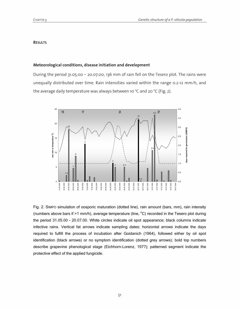
CHAPTER 3 Genetic structure of a P. viticola population
51
RESULTS
Meteorological conditions, disease initiation and development
During the period 31.05.00 – 20.07.00, 136 mm of rain fell on the Tesero plot. The rains were
unequally distributed over time. Rain intensities varied within the range 0.2-12 mm/h, and
the average daily temperature was always between 10 oC and 20 oC (Fig. 2).
0.2
4.2
2.5
12
2.22
3
3
6
2
10
1.2
0
5
10
15
20
25
31.0
5.20
00
02.0
6.20
00
04.0
6.20
00
06.0
6.20
00
08.0
6.20
00
10.0
6.20
00
12.0
6.20
00
14.0
6.20
00
16.0
6.20
00
18.0
6.20
00
20.0
6.20
00
22.0
6.20
00
24.0
6.20
00
26.0
6.20
00
28.0
6.20
00
30.0
6.20
00
02.0
7.20
00
04.0
7.20
00
06.0
7.20
00
08.0
7.20
00
10.0
7.20
00
12.0
7.20
00
14.0
7.20
00
16.0
7.20
00
18.0
7.20
00
20.0
7.20
00
mm
rain
or t
empe
ratu
re o C
0.0
0.5
1.0
1.5
2.0
2.5
3.0
3.5
4.0
days
requ
ired
for g
erm
inat
ion
(SIM
PO)
Fig. 2. SIMPO simulation of oosporic maturation (dotted line), rain amount (bars, mm), rain intensity
(numbers above bars if >1 mm/h), average temperature (line, oC) recorded in the Tesero plot during
the period 31.05.00 – 20.07.00. White circles indicate oil spot appearance; black columns indicate
infective rains. Vertical fat arrows indicate sampling dates; horizontal arrows indicate the days
required to fulfill the process of incubation after Goidanich (1964), followed either by oil spot
identification (black arrows) or no symptom identification (dotted grey arrows); bold top numbers
describe grapevine phenological stage (Eichhorn-Lorenz, 1977); patterned segment indicate the
protective effect of the applied fungicide.

CHAPTER 3 Genetic structure of a P. viticola population
52
Both on 04.06.00 and 07.06.00 conditions for primary infections were fulfilled (Goidanich,
1964; Hill, 2000). At the end of the previewed incubation period, however, on 11.06.00 and
15.06.00, respectively, no symptoms were recognized on our experimental plot.
The rain of 11.06.00 (maximal intensity: 3 mm/h; total: 6,6 mm in 7 hours) was supposed to
be the activating event to initiate the downy mildew epidemic. According to the SIMPO
simulation (Hill, 2000), oospores were mature to germinate and generate the very first
primary infections. As the Goidanich table estimates, 10 days after the rain of 11.06.00,
incubation time was over and first symptoms were recognized by the observer within the
poor grapevine vegetation (Eichhorn-Lorenz stage 21-22). Rains of 23-24.06.00 allowed both
new primary infections and sporulation of the recently appeared oil spots, which was
followed by secondary sporangia dispersal. Unlike the first infection date, SIMPO simulated 1.5
and 2 days for oosporic maturation on 23.06.00 and 24.06.00, respectively. The Goidanich
table (1964) estimates 9 days to complete incubation after each date. The rainy period 28-
30.06 did not induce infections, even though humidity could have been sufficient at least for
secondary cycles. On 04.07.00, heavy rains allowed both new primary infections and
secondary infections. Symptom appearance was expected on 14.07.00 following Goidanich
(1964), because oospores were mature to germinate (Hill, 2000) during the rain (Fig. 2). On
23.06.00, the Tesero vineyard showed 4 oil spots (Tes1s). From 9 to 21 days later, the
cumulative number of lesions increased to 75 and 97 lesions, respectively. Disease incidence
on vines (defined as number of infected vines per vineyard) already reached its maximum on
June, 2 (Table 3).
The epidemics in Navicello and San Michele started about one month earlier than in the
Tesero plot, and were characterized by more explosive development (data not shown).

CHAPTER 3 Genetic structure of a P. viticola population
53
Table 3. Genotype-specific contribution to the epidemic: identification date, P. viticola population,
number of observations and frequencies of the 15 genotypes identified in Tesero. Sampling size
(SS), cumulative sampling size (cum SS), number of infected vines (N inf vines), incidence (inc on
v) and cumulative incidence (cum inc on v) on vines.
genotype name 23.06.00 02.07.00 14.07.00 total
Tes1sa Tes2s Tes3s
evuzerca 1 (25)b 1
ezezomca 1 (25) 1
abewimna 1 (1.4)b 1
abewisma 1 (1.4) 1
aguverre 1 (1.4) 1
evuzemco 1 (1.4) 1
ezazinta 1 (1.4) 1
ezezumca 1 (1.4) 1
abegasra 1 (4.5)b 1
ebezemca 1 (4.5) 1
ezezemca 1 (4.5) 1
evivurro 1 (25) 20 (28) 21 (22)c
evuzemca 1 (25) 43 (60) 15 (68) 59 (61)
alovurma 1 (1.4) 1 (4.5) 2
evivusro 1 (1.4) 3 (14) 4
total genotypes 4 10 6 15
SS 4 71 22 97
Cum SS 4 75 97 97
N inf vines 4 18 7 22
Inc on vd 1.2% 5.5% 2.1% 6.7%
Cum inc on v 1.2% 6.7% 6.7% 6.7%
a: population name
b: frequency in % (100% refers to population size)
c: frequency in % (100% refers to 97 lesions)
d: infected grapes / tot grapes (N=328)
Genotype identification and population structure and dynamic
In the period 23.06.00 – 14.07.00, fifteen P. viticola genotypes were discriminated among 97
lesions collected (Table 3). Tes1s population consisted in 4 different genotypes causing 1 oil
CHAPTER 3 Genetic structure of a P. viticola population
54
spot each. Only two of the four genotypes identified were able to generate progenies, while
the remaining two were not re-identified again. Evuzemca is the genotype that contributed
the most to the epidemic: it was responsible for 60% of the total lesions on 02.07.00 and
68% on 14.07.00. Evivurro caused 20 lesions at the beginning of July (28% of total lesions)
but, afterwards, it was not able to multiply asexually again. 83% of the total lesions were due
to the combined pathogenicity of the two latter genotypes. On 02.07.00, eight new
genotypes (putative primary infections) contributed with a single lesion each to the
epidemic. Two of them were re-identified at the last sampling date whereas six genotypes
disappeared from the plot. Three new genotypes were identified on 14.07.00, causing minor
injury (13.5% of total lesions; Table 3). None of the genotypes identified in the Tesero
populations were identical to the valley populations (cross comparison not shown). While in
Tesero only 15 genotypes were identified among 97 lesions, in the valley populations almost
all lesions collected revealed a different genotype. The maximal number of clones was
observed in San Michele (Sdo) on 18.07.00, when 68 distinct genotypes were identified
among 76 sampled lesions (1.12 lesions/genotype).
Genetic variation
SSR analysis revealed different degrees of polymorphism among microsatellite markers of
the Tesero populations. Low diversities were observed at the loci BER and ISA (number of
alleles: k=2), while more alleles were recorded with the markers CES and GOB (kCES=6 and
kGOB=13; Table 4).
In Tesero, Nei’s (1973) expected heterozygosity ranged from a minimum of 0.25 (locus BER,
Tes3s) to a maximum of 0.75 (locus GOB and CES, Tes1s). Oosporic data sets (Tes2o, Tes3o and
TesTo) revealed similar (loci ISA and BER) or higher Hexp values than complete data sets. In all
the mountain data sets, a substantial heterozygosity excess for the loci ISA, GOB and CES
was observed, whereas a heterozygosity deficiency was exhibited by the locus BER. Although
the four valley populations do not differ considerably in Hobs and Hexp values from mountain
populations, we found a higher allele diversity (kISA=4; kGOB=30-38; kCES=10-15; kBER=2-3). This
pattern occurred even though we collected much less representatively (fewer oil spots in

CHAPTER 3 Genetic structure of a P. viticola population
55
regard to population size) in the valley populations than in the mountain populations (Table
4).
Considering the mountain “s”-populations (Tes1s, Tes2s and Tes3s), genotype frequencies at
all loci were in accordance with Hardy-Weinberg (HW) expectations only for the Tes1s
population (constituted by four individuals). Tes2s and Tes3s were obviously not in
equilibrium because of the effect of clonal multiplication of essentially two genotypes that
highly increased allele frequency of a sub set of alleles (Table 4). Clone-corrected total
populations (suffix “To”), comprehending valley populations, were generally in HW
equilibrium. Mostly the locus BER in Tes2o, TesTo, NamTo, SdoTo and SmiTo, and the locus
CES in TesTo, showed significant deviations from HW expectations.
Table 4. Summary of genetic variation within each of the three sampled P. viticola populations, the
clone-corrected Tesero data sets and the four total oosporic valley populations. Total N refers to the
number of individuals per population surveyed. SSR markers are listed in the headings. Stars
represent significant (“*”: p<0.05) and highly significant (“***”: p<0.001) deviations from Hardy-
Weinberg equilibrium.
Population number of alleles (k) heterozygosity (observed/expected)
N kISA kGOB kCES kBER ISA GOB CES BER overall
Tes1s 4 2 4 3 2 1.00/0.50 1.00/0.75 0.75/0.75 0.00/0.50 0.69/0.63
Tes2s 71 2 11 6 2 0.94/0.50*** 1.00/0.66*** 0.70/0.69*** 0.01/0.44*** 0.67/0.57
Tes3s 22 2 6 4 2 0.91/0.50*** 0.96/0.65*** 1.00/0.67*** 0.00/0.25*** 0.71/0.51
Tes2o 10 2 11 6 2 0.60/0.43 1.00/0.91 0.80/0.82 0.10/0.50* 0.63/0.67
Tes3o 6 2 6 4 2 0.67/0.47 0.83/0.85 1.00/0.79 0.00/0.33 0.63/0.61
TesTo 15 2 13 6 2 0.67/0.45 0.93/0.88 0.87/0.79* 0.07/0.39* 0.63/0.63
NacTo 120 4 34 15 2 0.50/0.50 0.81/0.90 0.78/0.75 0.13/0.17 0.56/0.59
NamTo 127 4 38 13 3 0.52/0.50 0.91/0.93 0.69/0.75 0.08/0.13* 0.55/0.58
SdoTo 104 4 30 10 2 0.57/0.49 0.90/0.94 0.66/0.60 0.12/0.16* 0.56/0.55
SmiTo 64 4 30 10 2 0.34/0.37 0.87/0.94 0.61/0.67 0.13/0.22* 0.49/0.55

CHAPTER 3 Genetic structure of a P. viticola population
56
Null allele frequency estimation
For the loci ISA, GOB and CES, null allele frequency for any population is seldom estimated
above 5%; ensuring a correct genotyping of the samples for those markers. The locus BER
shows instead about 25% probability of having null alleles in the clone-corrected mountain
populations and a maximum of 8% for the valley populations. All negative values for allele
frequencies were considered as equal to “zero” (Table 5).
Based on allele frequencies of oosporic populations, the theoretical number of different
genotypes (tG) that can be discriminated by means of the four SSR loci is approximately 104
(order of magnitude) for the Tesero total oosporic population and reaches about 100 times
higher values for the valley populations (Table 5). The theoretical occurrence of the genotype
that shows homozygosity for the most frequent allele at each SSR locus (tGo max) is for all
populations about 3*10-3 (Table 5). This genotype was identified exclusively in San Michele on
27.06.00 (Smi3s).
Table 5. Null allele frequency estimation of the 8 clone-corrected P. viticola Trentino populations for
all loci, theoretical maximal number of different genotypes (tG) and theoretical occurrence of the
most common genotype (tGo max).
Population ISA GOB CES BER tG tGomax
Tes1s <0a <0 <0 0.27 5.4*102 2.78*10-3
Tes2o <0 <0 <0 0.24 1.2*105 1.16*10-3
Tes3o <0 <0 <0 0.22 1.9*104 3.80*10-3
TesTo <0 <0 <0 0.21 1.7*104 1.68*10-3
NacTo 0 0.05 <0 0.03 4.3*106 4.19*10-3
NamTo <0 0.06 0.01 0.05 4.0*106 1.83*10-3
SdoTo <0 0.02 <0 0.04 1.5*106 2.68*10-3
SmiTo 0.01 0.03 0.03 0.08 1.5*106 2.61*10-3
a: slightly negative probabilities were noted by “<0”.

CHAPTER 3 Genetic structure of a P. viticola population
57
Population differentiation
No private allele was found in the Tesero oosporic population (Table 6). In 5 cases of 38, the
rarest alleles of the valley populations were detected within the Tesero populations. High
differences in allele frequencies were observed among valley and mountain pairwise
comparisons (as for GOB-385.7, CES-143.0, BER-179.2).
Table 6. Average allele sizes (bp) and allele frequencies of the total Tesero oosporic population
(TesTo) and of the four oosporic valley populations. Bold values refer to alleles occurring at the
highest frequency.
TesTo NacTo NamTo SdoTo SmiTo TesTo NacTo NamTo SdoTo SmiTo Locus GOB Locus ISA
205.8a - - - 0.005(-) 0.008(-) 118.3a - 0.071 0.075(-) 0.096 0.063(-)
210.0 0.133 0.263 0.177 0.144 0.148 137.1 - 0.054(-) 0.098 0.043(-) 0.070
260.7 - - 0.004(-) - - 140.2 0.333(-) 0.204 0.146 0.178 0.078
265.1 - - 0.004(-) - - 144.1 0.667 0.671 0.681 0.683 0.789
267.6 - - - 0.019 -
269.4 - 0.008 0.012 - -
271.4 - 0.004(-) 0.004(-) 0.005(-) - Locus CES
273.4 - 0.008 0.020 - 0.016
275.5 - 0.008 0.008 - - 143.0a 0.100 0.404 0.382 0.577 0.500
277.3 - 0.017 0.016 0.010 0.023 145.1 - 0.008 0.008 - -
279.3 - 0.004(-) - 0.005(-) - 154.9 - 0.004(-) - - -
281.5 - 0.013 0.012 - 0.008(-) 159.1 - 0.008 0.016 - 0.008(-)
285.0 - 0.017 0.008 0.043 0.047 161.1 - 0.004(-) - 0.029 0.016
289.7 - 0.017 0.028 0.005(-) - 163.1 - - 0.008 - -
291.9 - 0.004(-) - - - 165.1 - 0.004(-) - 0.005(-) -
294.1 0.033 0.042 0.055 0.034 0.016 167.2 - 0.017 0.016 0.014 0.023
298.2 - 0.050 0.067 0.029 0.039 169.4 - 0.017 - 0.005(-) -
300.2 - 0.017 0.016 - - 171.5 - 0.025 0.043 0.005(-) 0.008(-)
302.3 0.033 0.038 0.035 0.048 0.055 173.6 0.267 0.063 0.071 0.038 0.117
304.2 - - 0.016 0.010 - 175.4 0.300 0.254 0.303 0.250 0.258
306.6 - 0.013 0.020 0.043 0.039 177.7 0.067 0.108 0.083 0.058 0.047
310.5 0.033 0.038 0.039 0.043 0.023 179.5 0.233 0.063 0.051 0.019 0.008(-)
312.6 - - 0.004(-) - - 181.2 0.033 0.008 0.008 - 0.016
314.7 - 0.029 0.016 0.010 0.008(-) 183.6 - - 0.008 - -
318.9 - - 0.016 - - 185.8 - 0.013 0.004(-) - -

CHAPTER 3 Genetic structure of a P. viticola population
58
TesTo NacTo NamTo SdoTo SmiTo TesTo NacTo NamTo SdoTo SmiTo
Locus GOB Locus BER
323.0 - - - 0.014 - 179.2a 0.233(-) 0.092(-) 0.067 0.087(-) 0.125(-)
327.0 - 0.004(-) - - - 180.9 0.767 0.908 0.929 0.913 0.875
330.5 - - 0.004(-) 0.005(-) 0.008(-) 184.6 - - 0.004(-) - -
339.0 - 0.004(-) - - -
343.0 - - - - 0.008(-)
349.0 - - - - 0.031
355.9 - - - - 0.016
357.4 - 0.008 - - -
359.1 - - - - 0.008(-)
361.1 - 0.008 0.004(-) - 0.008(-)
365.2 - 0.017 0.028 0.024 -
367.2 - - 0.004(-) 0.005(-) 0.008(-)
369.3 - 0.075 0.055 0.130 0.078
371.3 - - 0.004(-) - -
373.3 - 0.058 0.098 0.058 0.023
375.6 0.033 0.013 0.012 0.058 0.070
377.7 0.067 0.079 0.102 0.053 0.086
379.5 - - 0.004(-) - 0.016
381.6 0.200 0.075 0.063 0.072 0.055
383.9 0.033 - - 0.010 -
385.7 0.267 0.025 0.016 0.063 0.078
388.1 0.033 - 0.004(-) 0.014 0.008(-)
389.8 0.033 0.021 0.016 0.034 0.047
391.8 0.033 0.008 0.004(-) 0.005(-) -
394.0 - 0.008 - - 0.016
396.1 - - - 0.005(-) -
398.3 0.067 0.004(-) - - -
400.5 - 0.004(-) 0.004(-) - -
412.3 - - - - 0.008(-)
414.4 - - 0.004(-) - -
(-) rarest allele sampled.
a: Average allele size was obtained after automatic allele scoring by the fragment analysis software
module (CEQ 2000XL, Beckman - Coulter, Fullerton, CA, version 4.2.0).

CHAPTER 3 Genetic structure of a P. viticola population
59
Fixation indices are measures of differentiation, which incorporate information on both the
frequency and identity of the alleles. In this study, Fst ranged from a low of 0 (estimates lower
than zero were treated as zero) to 0.179 (Table 7). In pairwise comparisons, low differences
were recorded among mountain “s”-populations (Tes1s, Tes2s and Tes3s; Fst max =0.019).
Pairwise tests of population differentiation calculated by FSTAT revealed no significant
differentiation among the three mountain “s”-populations sampled. P-values obtained after
4500 permutations were all >0.05. This means that the null hypothesis (no differentiation
between populations) can not be rejected (Table 7).
Considering total oosporic populations (suffix “To”), high diversity estimates among
mountain and valley populations were recorded (Fst max=0.086; TesTo/SdoTo). The lowest
diversity estimates were obtained after comparison between valley populations collected at
the same locality (SdoTo/SmiTo, Fst =0.005 and NacTo/NamTo, Fst =0.001). Significant
differences were obtained essentially when we compared populations collected from
different locations, but never when collected at the same location (SdoTo/SmiTo;
NamTo/NacTo; Tes1o/Tes2o/Tes3o/TesTo). Total Tesero oosporic population (TesTo) was
always significantly different from valley oosporic populations (Table 7).
Table 7. Estimates of pairwise Fst averaged over loci. “*” and “**” correspond to significance at the
5% and 1% nominal level after standard Bonferroni corrections, respectively .
Tes1s Tes2s Tes3s Tes2o Tes3o TesTo NacTo NamTo SdoTo
Tes2s -0.046
Tes3s -0.011 0.019
Tes2o -0.034 0.020 0.054
Tes3o -0.059 0.006 -0.004 -0.037
TesTo -0.041 0.020 0.024 -0.031 -0.051
NacTo 0.105 0.146** 0.118** 0.058* 0.026 0.052**
NamTo 0.106 0.151** 0.121** 0.061* 0.027 0.056** 0.001
SdoTo 0.147* 0.179** 0.149** 0.092** 0.060 0.086** 0.010** 0.012**
SmiTo 0.132* 0.170** 0.151** 0.067* 0.044 0.068** 0.011** 0.009** 0.005

CHAPTER 3 Genetic structure of a P. viticola population
60
Isolation by distance
There was a highly significant (p=0.003) positive relationship between pairwise Fst and
geographical distance or natural logarithm of geographical distance. Linear correlation
among the logarithm of geographical distance and the diversity estimator was low (R2=0.32;
y-intercept = 0.0205; slope = 0.0085; R2=0.32; Fig. 3). When mountain populations were
removed from the analysis, the relationship between Fst and geographical distance was still
statistically significant (p=0.000). Nevertheless the increase of Fst per difference of
geographical distance was six times lower than when including the Tesero populations
(R2=0.34; y-intercept = 0.0073; slope = 0.0014).
Fig. 3. Genetic distance (Fst) plotted against the natural logarithm of the geographical distance (km).
The dotted and the solid lines represent the best fit linear regressions when including valley
population only, and both valley and mountain populations, respectively. Triangles and squares
refer to pairwise comparisons within valley and between valley and mountain populations,
respectively.
-0.1
0
0.05
0.1
0.15
0.2
-6 -4 -2 0 2 4
ln (geo. dist / km)
Fst
-0.05

CHAPTER 3 Genetic structure of a P. viticola population
61
DISCUSSION
Impact of meteorological conditions to disease initiation and development
Even if meteorological conditions of the period 30.05.00 – 08.06.00 were suited for primary
infections (about 40 mm rain and a maximal rain intensity of 10 mm/h, temperature
between 10 and 20 oC), we did not observe any yellowish symptom after incubation time on
the Tesero plot. To explain this infection lack, we speculate that oospores were not yet
mature, even if SIMPO estimates one day to germination. Alternatively we could assume that
some few mature oospores did germinate, but macrosporangia were splash- or wind-
dispersed to plant material where infections are unlikely (cork, youngest leaves) and not
toward the poor vegetation. We observed one other rainy period with no impact on primary
and secondary cycles (28-30.06.00). Nevertheless, SIMPO simulation calculated about two
days for oospore germination. Probably the time lap required for germination was too long
and macrosporangia were produced when microclimatic conditions were not anymore
suitable for infection (no rains anymore). Rainy periods that played a major role both for
mildew initiation and asexual multiplication were characterized by at least 3 mm/h rain with
a maximum of 12 mm/h on 04.07.00. Rain intensity, combined with air turbulence, may
represent a key factor for macrosporangia dispersal. We assume that the majority of
germinating oospores lays trapped within at least 3/4 year old infected plant material (leaves
or berries) in the upper rhizosphere and that a raindrop with an impact higher than an
unknown threshold is required to disperse macrosporangia to the grapevine leaves. This
speculation seems to be disproved by data recorded during two rainy periods, on 04.06.00
and 07.06.00, when rain intensities were largely above 3 mm/h but, as already discussed,
oospores may not have been mature or were dispersed to non-targets.
Patterns of population differentiation
As expected for sexually recombining populations, the results in Table 4 confirm that all the
oosporic populations were mostly in Hardy-Weinberg equilibrium, with the exceptions of the

CHAPTER 3 Genetic structure of a P. viticola population
62
loci CES and BER. Locus CES had a heterozygote deficit and locus BER a heterozygote excess,
possibly generated by the presence of undetected null alleles in the sample of colonizers.
Indication of null allele presence is strongly suggested after appropriate analysis (Table 5) for
the locus BER. As soon as the probability of the presence of BER-null alleles reached 0.03, a
significant deviation from HW equilibrium was manifest (exception: Tes3o, which has only 6
individuals). Both populations Tes2s and Tes3s showed highly significant deviations from
Hardy-Weinberg expectations because of the dramatic increase in frequency of 1-2
genotypes (evivurro and evuzemca), indicating asexual reproduction and dissemination.
Three lines of evidence suggest that the heterogeneity of allele frequencies we observed is,
at least in part, the result of low gene flow on the spatial scale separating most sampled
populations. We first consider the observed pattern of isolation by distance, then the results
of the pairwise test of differentiation and, finally, some highlights of our more recent study.
The Mantel test detected an association between geographic and genetic distances in P.
viticola populations. Isolation by distance slopes departed from random expectations,
indicating that a significant pattern of isolation by distance applied to those populations.
The pattern resulted primarily from comparisons with the mountain populations. Twenty-
one of the 45 significant pairwise comparisons and 20 of the 22 Fst>0.02 involved the Tesero
populations. Although we clearly need to sample between the two valley localities to
determine the scale at which consistent differentiation becomes apparent, there seems to be
much differentiation at spatial distances of > 30 Km in the Trentino region. This initial
statistical approach provides the first indication of a geographically-restricted gene flow, not
only between valley and mountain, but also along the cultivated vineyard-rich valley.
Consistent with the isolation by distance test, the pairwise test of differentiation highlighted
significant genetic subdivisions between populations collected at different locations (among
Tesero, Navicello and San Michele). The finding of significant differences among the Tesero
populations and valley populations is likely an effect of the peculiar geographical location.
These findings suggest a nearly absent immigration (gene flow) from the nearest
neighbouring infected vineyards (30 Km) that would regularize allele number and frequency
among sites. Therefore we may consider all the genotypes of the Tesero population as a
single demographical unit. On the other hand, to find that the valley populations at a 42 Km

CHAPTER 3 Genetic structure of a P. viticola population
63
distance were genetically subdivided was unexpected, given that barriers to movements
between these locations are absent, that the grapevines cover 1/3 of the cultivated area and
that the disease has been established for a long time.
First disease identification was made in 1907 in San Michele (Rigotti, 1932). Again, but more
imperatively, this implies that the gene flow even between the two valley locations must be
limited. If gene flow exists, considering that 26 alleles out 80 were shared among the valley
populations, it may not be sufficient to avoid genetic isolation between populations settled
at 42 Km distance. It may, instead, play a major role in establishing patterns of genetic
homogeneity at more restricted local ranges (from ~0 to 500 m).
The findings of appropriate statistical analysis, finally, are consistent with our most recent
study, which surveyed 18 downy mildew epidemics in four central European countries (4685
lesions were collected, Gobbin et al., 2003, unpublished results). It essentially revealed that
secondary lesions caused by the same genotype are often very aggregated, such as at vine or
vineyard level (one or few disease clusters were observed). Only in a six-vine plot (Nv=6) did
clones of the same genotype succeed in colonizing the totality of the vines (at least one
lesion per vine), while, in the remaining 17 epidemics (of 18), we observed a colonization of
maximally 2/3 of the total number of vines (4 < Nv < 414; average surveying time: 1.5 months).
Based upon this aggregated spatial pattern of secondary lesions, we consider the
microsporangia wind-dispersal to be a very rare event, already at modest distances (> 50 m).
Rather, we speculated that the oospore-mediated gene flow may be more efficient, since
oosporic long viability period (at least five years, Hill GK, personal communication) would
permit more extensive disease propagation.
Consequently, both statistical tests and our more recent findings contradict current theories
about massive and long distance microsporangia wind-dispersal (Agrios, 1988; Blaise et al.,
1999; Lafon and Clerjeau, 1988) and suggest that primary and secondary lesions are likely of
autochthon origin or of spatially-restricted allochthon origin.
Given these issues, the simplest and more plausible explanation for the disease
establishment in Tesero is that it relies on the oospore import either from France with the
young plantlets or from the cultivated Adige valley through any kind of human transport. In
both cases, the disease-originating propagules would have experienced a human-mediated-

CHAPTER 3 Genetic structure of a P. viticola population
64
rather than a wind-mediated allochthon introduction. Having no indication of Alsatian
downy mildew alleles or allele frequencies at the studied four loci, we can neither support
nor discard the first hypothesis. Instead, considering that all the alleles found in Tesero were
identified in the valley, an import from the valley natural stock seems at least partially
supported.
Founder effect analysis
Although the small sample size of the TesTo population (15 individuals) may have created a
biased allele frequency distribution, several differences among TesTo and the four valley
populations are due to alleles that occur at high frequencies (Table 5). For instance, allele
GOB-385.7 occurs with high frequency in the TesTo population, but is almost deficient in the
four valley populations. Another example is CES-173.6: it is very abundant in TesTo but
present in lower frequency in the other populations. GOB-385.7 is the 11th most frequent GOB
allele (of 34) in NacTo but the 3rd most frequent (of 30) in SmiTo. Similarly for CES-173.6, it is
the 3rd and 4th most frequent in SmiTo (of 10) and NacTo (of 15), respectively. Microsatellite
variability of the Tesero populations is also characterized by substantial reductions of allelic
diversity in terms of the number of alleles per locus. Our case study revealed the loss of 33 of
38 low-frequency alleles (for instance: GOB-277.3; ISA-137.1; CES-165.1 absent in TesTo),
probably absent within the small number of effective population founders. Such abrupt
differences in allele frequencies and loss of alleles are typical consequences of founder
effects.
Implications for downy mildew epidemiology
In Tesero, 15 genotypes were identified within a vineyard area of 394 m2 (0.04 genotypes/m2)
while valley populations revealed a higher occurrence of genotypes: from 0.50 gen/m2
(NacTo) to 1.05 gen/m2 (SdoTo). In the valley we applied a grid sampling contrary to the
mountain plot were all lesions were sampled. A possible explanation may be that in the grid
sampling we failed in detecting clones and we biased consequently genetic diversity toward
an underestimation of lesions per genotype. This presumes that the secondary lesions are

CHAPTER 3 Genetic structure of a P. viticola population
65
restricted to an area smaller than the resolution of the grid (they are highly aggregated) or
that the secondary infections are a rare event. In any case those findings suggest that in San
Michele and Navicello autochthon oospore stocks may play a much more relevant role in an
epidemic than what is reported in the literature (Agrios, 1988; Blaise et al., 1999; Lafon and
Clerjeau, 1988) and generally assumed: primary infections are very numerous and occur
probably not exclusively during a short period at the beginning of the epidemic, as observed
in Tesero.
We observed a genotype-specific aptitude in producing secondary lesions. Thirteen out of 15
genotypes did not produce a relevant damage (1-3 lesions each), while only two genotypes
were responsible for 88% of the total lesions on 02.07.00 and one of them for 68% of the
total lesions on 14.07.00. It remains unclear why one of the most aggressive genotypes
(evivurro) on 02.07.00 was not able to undergo a further secondary disease cycle after
02.07.00. If epidemics in less atypical conditions show similar apparently stochastic and
genotype-specific asexual multiplications, it will be difficult to forecast the magnitude of
progeny simply by counting the number of sporulating lesions. Thus, it may be due to this
apparently stochastic asexual multiplication factors that epidemiological models often fail in
predicting the real relevance of secondary cycles. This research and future research, which
consider epidemics occurring in different locations, may bring new data to improve those
models and, consequently, disease management strategies.

CHAPTER 3 Genetic structure of a P. viticola population
66
ACKNOWLEDGMENTS
We express our thanks to many colleagues who have supported different areas of this work,
as data interpretators and doing practical lab work. We include Andrea Patocchi (ETH Zürich;
Switzerland), Artemis Rumbou (ETH Zürich, Switzerland), Bernd Loskill (FG Geisenheim,
Germany), Marc Raynal (ITV Blanquefort, France), and Mauro Jermini (RAC Cadenazzo,
Switzerland).

CHAPTER 3 Genetic structure of a P. viticola population
67
LITERATURE CITED
Agrios GN (1988) Plant pathology, 3rd edn, Academic press, San Diego, CA, pp: 313-319. Blaeser M, Weltzien HC (1979) Epidemiologische Studien an Plasmopara viticola zur Verbesserung der Spritzterminbestimmung. Zeitschrift für Pflanzenkrankheiten und Pflanzenschutz, 86:489-498. Blaise P, Dietrich R, Gessler C (1999) Vinemild: an application oriented model of Plasmopara viticola epidemics on Vitis vinifera. Acta Horticulturae, 499:187-192. Callen DF, Thompson AD, Shen Y, Philips HA, Richards RI, Mulley JC, Sutherland GR (1993) Incidence and origin of “null” alleles in the (AC)n microsatellite markers. The American Journal of Human Genetics, 52:922-927. Eichhorn KW, Lorenz DH (1977) Phänologishche Enwicklungsstadien der Rebe. Nachrichtenblatt des Deutschen Pflanzenschutzdienstes, 29:119-120. Fonseca DM, La Pointe DA, Fleischer RC (2000) Bottlenecks and multiple introductions: population genetics of the vector of the malaria in Hawaii. Molecular Ecology, 9:1803-1814. Gaggiotti OE, Lange O, Rassmann K, Gliddon C (1999) A comparison of two indirect methods for estimating average levels of gene flow using microsatellite data. Molecular Ecology, 8:1513-1519. Gobbin D, Pertot I, Gessler C (2003) Identification of microsatellite markers for Plasmopara viticola and establishment of high throughput method for SSR analysis. European Journal of Plant Pathology, 109:153-164. Goidanich G. (1964) Manuale di Patologia Vegetale. Edizioni agricole Bologna, Italy, p: 333. Goodman SJ (1997) RstCalc: a collection of computer programs for calculating estimates of genetic differentiation from microsatellite data and determining their significance. Molecular Ecology, 6:881-885. Goudet J (2001) FSTAT, a program to estimate and test gene diversities and fixation indices (v. 2.9.3). Journal of Heredity, 86:485-486. Gregory CT (1915) Studies on Plasmopara viticola. Official report of the session of the international congress on viticulture, P.P.I.E. San Francisco, California, July 12-13, pp: 126-150.

CHAPTER 3 Genetic structure of a P. viticola population
68
Hedrick PW, Gutierrez-Espeleta GA, Lee RN (2001) Founder effect in an island population of bighorn sheep. Molecular Ecology, 10:851-857. Hill GK (1990) Plasmopara Risk Oppenheim – a deterministic computer model for the viticultural extension service. Notiziario sulle Malattie delle Piante, 111:231-238. Hill GK (2000) Simulation of Plasmopara viticola oospore maturation with the model SIMPO. IOBC/WPRS Bulletin, 23 (4):7-8. Knapova G, Gisi U (2002) Phenotypic and genotypic structure of Phytophthora infestans populations on potato and tomato in France and Switzerland. Plant Pathology, 51:641-653. Lafon R, Clerjeau M (1988) Downy mildew. In: Compendium of Grape Diseases (ed. Pearson RC and Goheen AC), APS Press, St. Paul, Minnesota, USA. pp: 11-13. Lalancette N, Ellis MA, Madden LV (1988a) Development of an infection efficiency model of Plasmopara viticola on American grape based on temperature and duration of leaf wetness. Phytopathology, 78:794-800. Lalancette N, Ellis MA, Madden LV (1988b) A quantitative model for describing the sporulation of Plasmopara viticola on grape leaves. Phytopathology, 78:1316-1321. Nei M (1973) Analysis of gene diversity in subdivided populations. Proceedings of the National Academy of Sciences of the United States of America, 70:3321-3323. Pyri S, Luikart G, Cornuet JM (1999) bottleneck: a computer program for detecting recent reductions in the effective population size using allele frequency data. Journal of Heredity, 90:502-503. Raymond M, Rousset F (1995) GENEPOP (v.1.2): population genetic software for exact test and ecumenism. Journal of Heredity, 86:248-249. Rigotti R (1932) Rilievi statistici sulla viticoltura trentina: esperienze e ricerche della Stazione Sperimentale di S. Michele. Plate 7b. Vol.1. Scotoni A, Trento, Italy Rousset F (1997) Genetic differentiation and estimation and gene flow from F-statistics under isolation by distance. Genetics, 145:1219-1228. Schruft G, Kassemeyer HH (1999) Rebenperonospora. In: Krankheiten und Schädlinge der Weinrebe (ed. Thomas Mann Verlag ), Gelsenkirchen-Buer, Germany. pp: 14-17.
CHAPTER 3 Genetic structure of a P. viticola population
69
Spong G, Hellborg L (2002) A near-extinction event in lynx: do microsatellite tell the tale? Conservation Ecology, 6(1):15. Stryzik S (1994) Une deuxième génération de modèles systémiques : les potentiels systèmes. Vers une utilisation appuyée sur reseaux de stations météorlogiques. Groupe de travail "Biosystèmes en viticulture", Annales ANPP, 3e conférence internationale sur les maladies des plantes, pp :1447-1454. Wagner HW, Sefc KM (1999) IDENTITY 1.0. Centre for applied genetics, University of Agricultural sciences, Vienna. Available from http://www.boku.ac.at/zag/forsch/identity.htm. Wong FP, Burr HN, Wilcox (2001) Heterotallism in Plasmopara viticola. Plant Pathology, 50:427-432. Wright S (1969) Evolution and the Genetics of Populations, Vol. 2. The Theory of Gene Frequencies. University of Chicago Press, Chicago, IL.

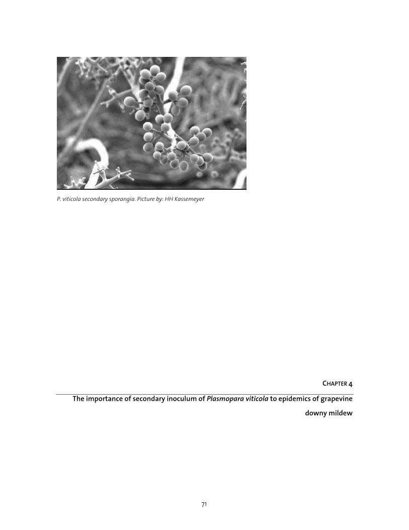
71
P. viticola secondary sporangia. Picture by: HH Kassemeyer
CHAPTER 4
The importance of secondary inoculum of Plasmopara viticola to epidemics of grapevine
downy mildew

CHAPTER 4 The importance of secondary inoculum
72
ABSTRACT
It is generally accepted, that epidemics of grapevine downy mildew, caused by Plasmopara
viticola, begins from a few germinating oospores. Once sporulating lesions from primary
infections are present, the pathogen has the ability to spread through secondary sporangia.
It is postulated from the literature, that the number of lesions generated by the secondary
phase greatly outweighs the oospore-derived primary lesions, but no quantitative data about
the population genetic structure are yet available. We assessed the magnitude of asexual
multiplication and quantified the spatial dispersion of secondary sporangia as function of
epidemic progression, by genotyping Plasmopara viticola samples. In a survey of downy
mildew populations from 2000 to 2002, 4685 P. viticola samples were collected from 18 plots
spread across central Europe. The samples were examined with a semi-automatic
microsatellite (SSR) analysis that identified more than 2300 site-specific P. viticola genotypes.
About 85% of all genotypes were sampled once or twice throughout the various epidemics.
In the 18 plots, only seven genotypes (0.3%) were identified more than 50 times. Three
particularly successful genotypes in causing disease through secondary cycles, showed
mostly a clustered distribution and a marked spatial autocorrelation. A further genotype
showed a random plot-scaled dispersion. Secondary sporangia migration distances per
secondary cycle were in the range from ~0 to 20 metres. We conclude that the secondary
sporangia have a generally low and heterogeneous degree of success in generating
secondary infections, which challenges the existing assumptions about disease epidemics.

CHAPTER 4 The importance of secondary inoculum
73
INTRODUCTION
D Downy mildew, caused by the heterotallic (Wong et al., 2001) diploid Oomycete
Plasmopara viticola (Berk. & Curt.) Berl. & de Toni, is the most important grape (Vitis vinifera)
diseases in temperate climates with spring rains. P. viticola overwinters as sexually produced
oospores in fallen leaves and berries. The current conception about the pathogen‘s
epidemiology postulates that the disease starts from a few germinating oospores that cause
primary/oosporic infections early in the grapevine vegetative season (Blaeser & Weltzien,
1979; Lafon & Clerjeau, 1988). After 5-18 days, depending on the temperature, the organism
produces microsporangia containing asexually produced zoospores (optimum: 18oC and
saturating humidity) (Agrios, 1988). The first infections are therefore followed by successive
asexual cycles, where the secondary sporangia cause secondary/clonal infections and lead to
an explosive disease progress (Schruft & Kassemeyer, 1999). The dispersal of the disease is
believed to rely on the migration of secondary sporangia, which are thought to travel long
distances in a short time (Blaise et al., 1999; Lafon & Clerjeau, 1988). To our knowledge, no
quantitative data about migration distances of specific genotypes are yet available.
In order to predict the risk of secondary or primary infections, weather-driven
epidemiological models have been proposed. Most of these models are based on the
assumption that an epidemic starts from a restricted number of oosporic infections,
followed by massive clonal multiplication (Lalancette et al., 1988a,b; Blaise et al., 1999). A few
models are based primarily on the simulation of the germination dynamic of oospores and
consider them as the only responsible for the whole epidemic (Hill 1990; Hill 2000; Strizyk
1994). However, models often fail in predicting the real quantitative development of
epidemics, which restricts their use in practice or leads to overestimation of infection risk. At
the current knowledge status, models can not be significantly improved without separate
quantitative modelling of sexual and asexual phases (M Jermini and M Raynal, personal
communication).
Spatial pattern of disease results from the interaction between physical, biological and
environmental factors. Several statistical methods for defining spatial relationships, such as
indexes of dispersion or calculation of variances of blocked quadrats, have been developed

CHAPTER 4 The importance of secondary inoculum
74
(Charest et al., 2002). These calculations do not consider the physical location of the quadrat
or its relationship with other sample sites. To overcome this deficiency, geostatistical
analyses have been developed (Charest et al., 2002). Geostatistic, originally developed for
mining (Barker & Lally, 1993), has already been applied in plant pathology to quantitatively
characterize spatio-temporal patterns of disease (Xiao et al., 1997; Turecheck & Madden,
1999; Van der Lande & Zadocks, 1999). Geostatistical analysis can be used to detect spatial
dependency for continuous and discrete variables. Spatial dependence could be analysed
directionally or omnidirectionally with semivariograms, which quantify spatial dependence
by measuring variations between samples separated by a vector: the “lag distance” (Savary
et al., 2001, Wu et al., 2001).
In this study, we combined the genetic (Gobbin et al., 2003a) and statistical knowledge, in
order to 1) determine which proportion of total P. viticola genotypes undergoes secondary
disease cycles, 2) quantify the magnitude of secondary sporangia-derived asexual progeny,
and 3) quantify the spatial dispersion of particularly successful genotypes in generating
secondary lesions as a function of epidemic progression. In order to reduce single site
variability, in terms of particular macro and microclimatic conditions, grape responses to
disease attack, pathogen aggressiveness etc., we selected 18 sites across central Europe
where to survey downy mildew epidemics.

CHAPTER 4 The importance of secondary inoculum
75
MATERIALS AND METHODS
Vineyard locations and epidemics surveyed
Eighteen plots (17 not treated and one, Cum, treated four times with fungicides) were
selected within four European-wine-producing countries (Germany, France, Italy and
Switzerland; Fig. 1). Naturally occurring downy mildew epidemics were surveyed during years
2000-2002 within those plots. The survey period started as soon as the first lesions (also
called oil spots) were noticed and stopped when downy mildew generated a mosaic pattern
which impeded the collection of distinct lesions. On average, the survey period lasted 1.5
months and ended generally in July or August. One sample consisted in 0.5 - 1 cm2 of every
identifiable lesion (corresponding to approx. 1/3 to 1/2 of the total lesion surface) including
up to 0.5 cm2 of healthy leaf tissue. The remaining part (1/2 to 2/3) of the lesion was not
sampled to allow the survival of the genotype in the plot. The exact location of each lesion
within the plot was recorded according to vine and row number. Oil spots were collected on
2 to 22 sampling dates per plot throughout the 18 epidemics; in total, for all plots and all
sampling dates, 83 independent samplings were performed (Table 1). Two different sampling
strategies were used: total- and partial- sampling strategies (TSS and PSS, respectively). The
total sampling strategy was used when, on average, less than 5 oil spots per vine were
present. Using this strategy all oil spots were collected as soon they were visible. A partial
sampling strategy was performed as an alternative to total sampling, when more than 5 oil
spots per vine were present. Using PSS, 1 to 3 oil spots per vine were sampled.
When the total sampling strategy was applied at least on two sampling dates within the
same plot throughout one epidemic, we considered the total downy mildew population
(pooled individuals collected on all sampling dates) to be totally sampled (TSS; Table 1). When
the TSS was used on one sampling date (or none, as in Wad) and the PSS on all the remaining
sampling dates, we considered the total P. viticola population as partially sampled (PSS, Table
1). Hereafter TSS or PSS will refer to the sampling strategy applied to the 18 total populations
and not to the 83 independent samplings.

CHAPTER 4 The importance of secondary inoculum
76
As in Was a single vine was infected, we sampled all lesions (TSS) on any sampling date and
we recorded their positions according to a reference system defined by six sectors (top,
medium, low and left, right vine sectors, Fig. 4).
Figure 1 Locations of the 18 downy mildew populations surveyed during years 2000-2002. 1: Biasca
(Bia), 2: Blanquefort (Bla), 3;4: Cugnasco (Cut and Cum), 5: Gaillac (Gai), 6: Navicello (Nam), 7:
Perroy (Per), 8: Stäfa (Sta), 9: Wädenswil (Wad), 10: Bommes (Bom), 11: Carpineta (Car), 12:
Erbach (Erb), 13: Geisenheim (Gei), 14: Lorch (Lor), 15: Navicello (Nac), 16: Tesero (Tes), 17: Vic
(Vic) and 18: Wädenswil (Was).
1,3,42 10
5
6,15 16
11
12,13,14
7, 178,9,18

CHAPTER 4 The importance of secondary inoculum
77
Table 1 Vineyard location (site number, site abbreviation, site name in full and nation), training system, grape variety, number of rows (R), distance
between rows (dr), number of vines per row (V), distance between vines in a row (dv), total vines (N v), plot area (A), sampling dates (S date), sampling
strategy (SS), sampling size (Nobs), number of different genotypes (Ngen), number of single genotypes (genotypes that occurred once all over the surveying
period; Nsgen), name of the most frequent genotype (MFG name), occurrence of the most frequent genotype (Nobs MFG), name of the (SMFG name) and
occurrence of the SMFG (Nobs SMFG). Bold characters refer to the main sampling strategy applied, to the total number of lesions collected (tNobs), of
genotypes identified (tNgen), of single genotypes identified (tNsgen) of MFG identifications (tNobs MFG) and of SMFG identifications (tNobs SMFG).
Vineyard loc training syst R V N v MFG name SMFG name grape var dr dv Aa S date SS b Nobs Ngen Nsgen Nobs MFG Nobs SMFG
1- Bia evawasma ibevasca Biasca Guyot 2 21 42 26.5.00 TSS 27 26 18 0 1
Switzerland Merlot 1.75 m 1.25 m 92 m2 18.6.00 PSS 96 70 48 5 5
30.6.00 PSS 101 64 36 12 8
13.7.00 PSS 90 67 42 3 2
tot pop PSS 314 190 144 20 (6.4%)c 16 (5.1%)d
2- Bla ebebissa ebetassa Blanquefort Doub Guyot 4 70 280 10.5.00 TSS 36 30 22 0 2
France Merlot 1.5 m 1 m 420 m2 31.5.00 PSS 100 85 53 2 0
16.6.00 PSS 189 151 94 7 5
07.7.00 PSS 106 85 45 1 2
07.8.00 PSS 126 93 62 4 0
tot pop PSS 557 363 276 14 (2.5%) 9 (1.6%)
3- Cut alovispa ibetosna Cugnasco Guyot 1 6 6 07.6.01 TSS 1 1 1 0 0
Switzerland Merlot 2 m 1.2 m 14 m2 25.6.01 PSS 42 17 10 10 14
23.7.01 PSS 135 56 39 34 21
tot pop PSS 178 69 50 44 (23.5%) 35 (18.7%)
4- Cum alovispa ebebesra Cugnasco Guyot 4 61 244 07.6.01 TSS 17 9 5 0 6
Switzerland Merlot 2 m 1.2 m 586 m2 25.6.01 PSS 41 21 17 0 20
23.7.01 PSS 340 137 78 45 0
29.8.01 PSS 86 50 27 10 0
tot pop PSS 484 193 127 55 (11.4%) 26 (5.4%)

CHAPTER 4 The importance of secondary inoculum
78
5- Gai abebessa aveyusla Gaillac C Royat 4 21 79 05.6.00 PSS 21 10 5 10 2
France Duras 2.5 m 1 m 210 m2 14.6.00 PSS 26 16 12 9 3
tot pop PSS 47 22 17 19 (40%) 5 (10.6%)
6- Nam avavissa igigomma Navicello Guyot 5 21 105 22.5.00 TSS 2 2 1 0 0
Italy Merlot 2 m 1 m 210 m2 30.5.00 PSS 18 17 12 0 0
21.6.00 PSS 57 47 40 5 3
06.7.00 PSS 86 81 74 0 0
tot pop PSS 163 142 127 5 (3.0%) 3 (1.8%)
7- Per ebesossa efoganta Perroy S Guyot 4 26 88 30.5.00 PSS 85 41 18 17 2
Switzerland Chasselas 2 m 0.8 m 166 m2 29.6.00 PSS 131 53 26 26 17
11.8.00 PSS 109 49 22 19 4
tot pop PSS 325 108 66 62 (19.0%) 23 (7.1%)
8- Sta evivusme abevisme Stäfa Guyot 4 20 73 27.6.00 PSS 72 44 22 7 11
Switzerland RxS 2.1 m 0.9 m 134 m2 26.7.00 PSS 117 65 28 4 9
18.8.00 PSS 139 60 29 30 11
tot pop PSS 328 129 79 41 (12.5%) 31 (9.5%)
9- Wad ozewisra ebezesma Wädenswil Guyot 5 3-15 47 21.6.00 PSS 54 21 10 19 6
Switzerland RxS 1.9 m 1 m 89 m2 26.7.00 PSS 73 29 17 35 3
tot pop PSS 127 43 27 54 (42.5%) 9 (7.1%)
10- Bom übetosca azowirma Bommes D Guyot 7 40-69 414 <27.6.01e - 1 1 0 1 0
France Sémillon 1.5 m 0.9 m 559 m2 27.6.01 TSS 63 3 1 60 0
10.7.01 TSS 18 9 2 4 0
24.7.01 PSS 58 15 5 25 5
27.8.01 PSS 53 27 20 22 5
tot pop TSS 193 41 28 112 (58.0%) 10 (5.2%)
11- Car afevissa afowusba Carpineta wild 3 23 57 25.5.01 TSS 18 15 11 1 0
Italy Sangiovese 2.5 m 2 m 345 m2 08.6.01 TSS 49 31 17 8 1
27.8.01 TSS 57 45 31 0 3
tot pop TSS 124 84 59 9 (7.3%) 4 (3.2%)

CHAPTER 4 The importance of secondary inoculum
79
12- Erb afolonna dgulepma Erbach Halbbogen 3 12 36 18.5-6.7.00 f TSS 230 199 136 0 9
Germany Riesling 2 m 1.1 m 79 m2 10.7.00 TSS 11 9 5 2 0
27.7.00 TSS 1 1 1 0 0
01.8.00 TSS 45 21 6 7 0
tot pop TSS 287 192 148 9 (3.1%) 9 (3.1%)
13- Gei egigusra jlomaspa Geisenheim Halbbogen 3 13 39 26.5.00 TSS 7 2 0 3 0
Germany RxS 1.8 m 1.2 m 84 m2 31.5.00 TSS 7 2 0 6 0
05.6.00 TSS 30 8 2 10 4
19.6.00 TSS 141 25 15 55 31
06.7.00 TSS 21 8 3 5 5
tot pop TSS 206 33 20 79 (38.2%) 40 (19.4%)
14- Lor afevimca avuzomme Lorch Rundbogen 3 12 36 05.6.00 TSS 14 9 5 6 0
Germany Riesling 2 m 1.3 m 93 m2 06.6.00 TSS 3 3 3 0 0
16.6.00 TSS 57 33 19 16 0
19.6.00 TSS 45 38 24 2 0
20.6.00 TSS 148 107 81 16 4
21.6.00 TSS 34 22 16 0 13
27.6.00 TSS 60 49 36 7 1
tot pop TSS 361 228 184 47 (13.0%) 18 (5.0%)
15- Nac ymatosmo abebessa Navicello Sin.Pergola 4 33 132 15.5.00 TSS 6 6 5 0 0
Italy Chardonnay 2.8 m 0.8 m 296 m2 22.5.00 TSS 27 19 12 6 2
30.5.00 TSS 414 351 315 13 6
tot pop TSS 447 370 332 19 (4.3%) 8 (1.8%)
16- Tes evuzemca evivurro Tesero Guyot 16 18-23 328 23.6.00 TSS 4 4 2 1 1
Italy Chardonnay 1.5 m 0.8 m 394 m2 02.7.00 TSS 71 10 6 43 20
14.7.00 TSS 22 6 3 15 0
tot pop TSS 97 15 11 59 (60.8%) 21 (21.6%)
17- Vic abedussa abegisma Vic Pinot noir 6 25 136 11.8.00 TSS 74 45 15 8 3
Switzerland Guyot S 1.65 m 0.8 m 180 m2 25.8.00 TSS 262 97 40 25 16
tot pop TSS 336 114 55 33 (9.8%) 19 (5.7%)

CHAPTER 4 The importance of secondary inoculum
80
18- Was ezazerma emizorma Wädenswil Guyot 1 4 4 01.6.02 TSS 1 1 0 1 0
Switzerland RxS 1.9 m 1 m 8 m2 10.6.02 TSS 25 1 0 25 0
16.6.02 TSS 85 6 4 79 2
tot pop TSS 111 6 4 105 (94.6%) 2 (1.8%)
a: Plot area was calculated as R*dr*V*dv [m2].
b: TSS: total sampling strategy; PSS: partial sampling strategy.
c: Pecentage refers to the MFG-derived disease severity: DS%MFG (tNobs MFG / tNobs).
d: Pecentage refers to the SMFG-derived disease severity: DS%SMFG (tNobs SMFG / tNobs).
e: No sampling was performed prior to 27.06.01. An “open” date refers to the putative appearance of the very first primary infection caused by the MFG
übetosca.
f: A summary of the first 19 samplings performed in Erbach is shown. SMFG dgulepma was identified 6 times on 6.06.00, once on 09.06.00 and twice on
06.07.00.

CHAPTER 4 The importance of secondary inoculum
81
Sample processing and genotype identification
For genotyping the collected samples, we used automated high throughput DNA extraction,
PCR amplification of the four polymorphic P. viticola specific SSR loci BER, CES, GOB and ISA,
sequencer based fragment analysis and automatic allele scoring (Gobbin et al., 2003a). P.
viticola genotypes were defined as strains that differed by at least one allele in their SSR
profiles. Genotypes were named by merging 8-letters (for instance: evawasma and ibevasca
identified in Biasca, Table 1), according to a SSR allele coding methodology not described in
this paper. We considered that each oospore contains a single nucleus (Gregory, 1915; Gobbin
et al., 2003a) that it is asexually inherited by the progeny (secondary lesions). We assume
that asexual cycles did not alter the microsatellite allele pattern. Therefore, two oil spots
showing identical allele pattern (same genotype) were interpreted as clonal progeny,
deriving from the same oospore. Different genetic profiles of two oil spots were interpreted
as derived from independent oosporic infections. The first appearance of a genotype was
considered as an oosporic-derived primary lesion. Any subsequent observation of the same
genotype was interpreted as a secondary lesion.
Data and distribution analysis
Independently for each of the 18 plots we pooled all the individuals collected on the 2 to 22
sampling dates. The total number of individuals (tNobs) and the total number of genotypes
(tNgen) were calculated. The number of genotypes that were identified the same number of
times (tNobs=X; 1≤X≤112) throughout the survey period was determined and the frequency of
every occurrence class (FtNobs=x) was calculated. The genotypes occurring once throughout the
survey period (tNobs=1) were defined as single genotypes. The genotypes occurring at the
highest frequency were defined as most frequent genotypes (MFGs), while genotypes
occurring at the second highest frequency were defined as second most frequent genotypes
(SMFGs). In this study, disease severity was defined as the number of lesions, or observations
(Nobs), identified in a spatial unit (plot or vine). The contribution of any genotype(s) to the
total disease severity, was calculated by dividing the number of lesions generated by the
considered genotype(s) by the total severity and expressed in percentage (DS%). Scatterplots
showing data distribution and MFG locations in the plots were constructed by means of

CHAPTER 4 The importance of secondary inoculum
82
Systat (version 10, SPSS Inc., 2000). The same software was used to construct ELL Gaussian
bivariate confidence ellipses (p=0.68). Two-sided t-tests were performed in a Microsoft Excel
spreadsheet (version 2002). In order to evaluate the oil spot distribution pattern, we
employed the variance-to-mean ratio (v/m), which gives an indication of the type of
distribution (regular, random or clustered) of the data (Campbell & Madden, 1990). To
calculate this index, we used individual grapevines as spatial units, or quadrats, because they
are regularly planted within plots. For every vine, the cumulative number of lesions caused
by the MFG at a defined date (cNobs MFG) or by any other genotype (cNobs) was calculated.
Variance and mean variables of cNobs MFG and cNobs per vine were calculated for every plot. We
analysed the variation of the v/m ratio over time for three plots Bom, Gei and Tes, where
clones of MFG were identified at least 50 times (tNobs MFG > 50) and a total sampling strategy
(TSS) was performed (Table 1). When v/m is <1, =1, or >1, the pattern of distribution is
considered regular, random or aggregated, respectively. The Poisson probability distribution
was used to test whether a MFG spatial pattern of distribution was random or non-random,
based on cNobs MFG per vine. When the frequency of lesions distribution corresponded to the
expected frequency distribution of Poisson, determined by the �2 test, the spatial distribution
was considered to be random. Alternatively, a non-random distribution was interpreted
either as aggregated or regular (Charest et al., 2002).
Geostatistical analyses
Semivariogram analysis was performed on the natural logarithm of the cumulative number
of MFG-derived lesions incremented by one (ln[cNobs MFG +1]) and associated spatial locations
(row direction and direction perpendicular to row, or, by convention, North and East
directions, respectively; all extensions were expressed in metres defining by co-ordinate (0 m
; 0 m) the location of vine 1 in row 1), using software GS+ for Windows (version 5.1, RockWare
Inc., 2003). We applied a transformation from cNobs MFG to ln[cNobs MFG +1] in order to reduce
semivariance among lag increment classes and to obtain better fit of models. Lag distances
were set to 8 m (Gei) and 10 m (Bom and Tes), which are less than half the maximum
distance between sample pairs, while lag increments were set to the plot specific distances
between vines increased by 10 cm (dv, Table 1). In GS+, both anisotropic and isotropic

CHAPTER 4 The importance of secondary inoculum
83
semivariograms were generated. For anisotropic semivariograms, four conventional
directions were considered: North (row direction, angle = 0o), North-East (45o), East (direction
perpendicular to rows, 90o) and South-East (135o), while for isotropic semivariograms, all
angles between 0o and 360o were considered. The best-fitting models were selected among
the five provided by GS+, according to the highest R2 value and the lowest sum of squares.

CHAPTER 4 The importance of secondary inoculum
84
RESULTS
Differential genotype contribution to the epidemic
Although plot locations were spread across central Europe, sampling was performed in
different years (mostly in 2000) and meteorological conditions differed remarkably (data not
shown), downy mildew symptoms appeared approximately at the same time period (mid
May to end of May). In a few cases, the disease first appeared in June (Bom, Wad, Tes and
Sta) or even in August (Vic). The survey periods lasted on average 1.5 months and ended
generally in July or August, when downy mildew started generating mosaic patterns which
impeded the collection of lesions. From the nine plots where TSS was applied, 2162 half oil
spots were successfully genetically analysed, revealing the presence of 1083 genotypes. From
the remaining nine plots where PSS was applied, 2523 symptoms (half oils spots) were
analysed and 1259 different genotypes were distinguished. In summary, among the 4685 oil
spots considered, 2342 genotypes were identified (Table 1).
After grouping of the genotypes occurring the same number of times throughout one
epidemic (tNobs=X) into genotype frequency classes (FtNobs=x), we showed that single
genotypes (tNobs=1) often constituted the greatest fraction of the individuals collected. On
average, 71% of all genotypes of the 18 total populations, assessed both after PSS (Fig. 2a) and
TSS (Fig. 2b), were identified only once throughout the survey period. The lowest percentage
was recorded in Vic, where single genotypes were 48% of all genotypes; the highest was at
Nac, when single genotypes comprised 90% of all genotypes. On average, over the nine
populations sampled after PSS, single genotypes were responsible for 37% of the total
disease severity (st.dev: 19%; Fig. 2c). In the other populations (TSS, Fig. 2d), single genotypes
caused an average of 31% of the total disease severity (st.dev: 25%). A high proportion of
single genotypes was observed independently from the sampling date (Fig. 3). Even on the
latest sampling dates, in seven populations (Bia, Bla, Gai, Nam, Car, Lor and Nac) more than
40% of new single genotypes were found.
Genotypes that were identified twice (tNobs=2) in the same plot throughout the season
(either twice on the same sampling date or once on two sampling dates), were, on average,
15% and 13% of the total number of genotypes identified, after PSS and after TSS, respectively

CHAPTER 4 The importance of secondary inoculum
85
(Fig. 2a and 2b). The proportion of disease severity caused by those genotypes was on
average 13.7% (st.dev: 2.2%) after PSS and 11.0% (st.dev: 8.7%) after TSS (Fig. 2c and 2d).
The Euclidean distances between the two clones of the genotypes that were identified on
the same sampling date were shorter than the distance between the clones of the genotypes
collected once on two sampling dates (tNobs=2). 107 genotypes were identified twice on the
same sampling date (tNobs=2; 214 lesions). The two clones of each of the 107 genotypes were
located in 22 case (20.6%) on the same leaf, in 19 cases (17.8%) on two different leaves of the
same vine, in 12 cases (11.2%) on two neighbouring vines of the same row, in 2 cases (1.9%) on
two vines of the same row with a vine in-between and in 2 cases (1.9%) on two vines laying
vis-à-vis of two adjacent rows. That indicates approximately the half of all genotypes (49.5%)
are located maximally at about 1m apart while the other half at farther distances. The
longest distance between two clones of the same genotype, 15 m, was measured in Vic,
where the genotype ewavisna, was identified on 25.08.00 (2nd sampling) on the vines 21/4
and 2/5 (vine/row). 268 genotypes were identified once on two sampling dates (tNobs=2; 536
lesions). OIn none of the 268 cases, none were colonizing the same leaf (just because we
never sampled on previously sampled leaves), in 24 cases (8.9%) the two clones of the same
genotype were colonizing two different leaves of the same vine, in 20 cases (7.5%) they were
colonizing two neighbouring vines of the same row, in 11 cases (4.1%) they were colonizing
two vines of the same row with a vine in-between and in 9 cases (0.3%) they were colonizing
two vis-à-vis vines of two adjacent rows. The remaining 76.1% of the clones was at more than
3m distance. The longest distance between two clones of the same genotype, 67 m, was
measured in Blanquefort, where the genotype ebenossa, first identified on 10.05.00 on
vine14/6, was found on 07.08.00 on vine 81/3.
Based on TSS, only 15 of 1083 genotypes (1.4%) were identified more than 10 times, while 8
(0.7%) were identified more than 20 times. The same trend was found after a partial
pathogen collection (PSS), when, out of 1259 genotypes identified, 23 (1.8%) and 11 (0.9%)
genotypes, were identified more than 10 times and more than 20 times, respectively. The
proportion of total disease severity generated by those particularly successful genotypes
reached 20% in seven cases and 50% in three cases.
CHAPTER 4 The importance of secondary inoculum
86
MFGs were uniformly distributed within the populations surveyed, independent from the
collection strategy applied. Twelve genotypes that were identified between 21 and 50 times
belonged to 8 populations (avg: 0.67; min: 0; max: 3 genotypes per population). Seven
genotypes that were identified more than 50 times belonged to seven distinct populations.
Populations that included the most successful genotypes (tNobs≥21) were: Gei (the MFG was
identified 79 times + the SMFG was identified 40 times), Tes (59 + 21), Per (62 + 23), Cum (55 +
26) and Cut (44 + 35) (Table 1 and Fig. 3).
FtNobs=X and DS% data distribution within occurrence classes (tNobs=X) are equally described
independently from the sample collection method (TSS or PSS; Fig. 2). Non significant
differences (p>0.05 after t-tests) were always obtained when comparing the averages of
FtNobs=X and DS% for 1≤ tNobs ≤9. No comparisons were possible after tNobs ≥10 because of the
lack of a sufficient data set.

CHAPTER 4 The importance of secondary inoculum
87
Figure 2abcd. Frequency (FtNobs=x, Fig. 2a and 2b) and percentage of total disease severity (DS%);
Fig. 2c and 2d) of genotype occurrence classes (x-axis). The genotypes that were identified the
same number of times throughout the survey period were classified into occurrence classes
(tNobs=1,2,3…112). Square and round symbols refer to data collected by PSS and TSS, respectively.
All data points were calculated independently for each of the 18 total populations surveyed.
F tNobs
Occurrence class (tNobs)
DS%
1 10 100 1 10 100
2a 2b
0.6
0
0.8
1
0.4
0.2
60
0
80
100
40
20
2c 2d

CHAPTER 4 The importance of secondary inoculum
88
Figure 3. Cumulative proportion of disease severity (y-axis; DS%) caused by the most frequent
genotype (MFG), the second most frequent genotype (SMFG), all other genotypes (other gen) and
single genotypes as a function of epidemic progress. The survey periods (x-axis) spans from 10.05
to 27.08 on the sampling year, either 2000 or 2001 or 2002 (Table 1).
Downy mildew dispersion strategies
Based on the epidemics studied, P. viticola genotypes showed five distinct dispersal patterns:
1) clonal multiplication on single, or few, vines (Car: afevissa, Cum: ebebesra, Gei: jlomaspa,
Lor: avuzomme, Tes: evivurro and Was: ezazerma); 2) clonal multiplication on single, or few,
vines followed by plot-scaled dispersion (Bia: ibevasca and evawasma, Bom: übetosca, Cum
and Cut: alovispa, ibetosna, Nac: ymatosmo, Per: efoganta, Vic: abegisma); 3) multi-cluster
plot-scaled dispersion without previous clonal multiplication on a few vines (Lor: afevimca,
Tes: evuzemca); 4) random plot-scaled dispersion without previous clonal multiplication on a
MFG
Bom Car Erb Gei Lor
Nac Tes Vic Was
Bia Bla Cut Cum Gai
Nam Per Sta Wad
single gen other gen SMFG
10.05 05.07 26.08 07.09
cNobs(%)
100 80 60 40 20

CHAPTER 4 The importance of secondary inoculum
89
few vines (Gei: egigusra), and 5) minor clonal multiplication and dispersal. The last class
included 99% of the genotypes. The MFGs found in Gai, Per, Sta, Vic and Wad were not
strictly classified into any of these four categories because, on the first sampling date, they
were already found to be partially plot-scale dispersed. Therefore, due to the lack of a
restricted focus, they would eventually be classified into the third or fourth class.
In the following four case studies, we examined four dispersed patterns by genotypes that
were identified at least 50 times each: ezazerma (strategy 1), übetosca (strategy 2), egigusra
(strategy 3) and evuzemca (strategy 4).
Strategy 1: clonal multiplication on a single vine
In Wädenswil (Was) a heavily sporulating oil spot (genotype ezazerma) was detected on
01.06.02 on a leaf located within the medium-right sector of a vine (Fig. 4 and Table 1). After
an asexual disease cycle, on 10.06.02, we observed a spatially restricted infection focus
generated by the same genotype in the immediate vicinity of the first infected leaf. A total of
25 new oil spots were detected on six adjacent newly infected leaves: 14 lesions on two leaves
within the left-medium sector (12 and 2 lesions, respectively) and 11 lesions on four leaves
within the right-medium sector (3, 3, 3 and 2 lesions, respectively). No other genotype was
identified among the 25 oil spots. On 16.06.02, presumably after a new secondary cycle, 85
lesions were detected within the same vine. Five additional genotypes were identified,
suggesting the occurrence of new primary infections. One of them (emizorma) was already
present twice (2 clones) on a unique leaf, suggesting a double infection by two (or more?)
zoospores released from the same macrosporangium (oospore). The other four single
genotypes were found on four distinct leaves. Ezazerma was found 79 times, colonizing 23
new leaves and sharing two of them with other two genotypes. On average, it produced 3.43
lesions per leaf (st. dev:1.8; max: 8 m; min: 1 lesions/leaf). Forty-one lesions were distributed
within the medium and the highest left sector, while the remaining 38 were located within
the right sectors. In summary, 50 lesions (on 14 leaves) were found on the left side of the
wine, while on the right vine side 55 lesions (on 16 leaves) were found, mostly (68%)
distributed within the medium sectors. Secondary sporangia did not migrate more than 1
meter after two secondary cycles, never reaching nearby vines that were perfectly healthy.

CHAPTER 4 The importance of secondary inoculum
90
Figure 4. Cumulative spatio-temporal dispersion pattern of the most frequent genotype in
Wädenswil (ezazerma). The single vine infected is represented by a bi-dimensional scaled
rectangle, as if it was observed from a neighboring vine on the same row. Dimensions on x-axis
represent left-side and right-side vine extensions, while y-axis represents vine height (in metres).
The grapevine was divided into six sectors (left and right, top, medium and low sectors). Dot size is
proportional to the natural logarithm of (Nobs MFG+1) and represents the number of MFG observations
per infected leaf. The position of infected leaves was assigned randomly within the corresponding
sector. Uninfected leaves and leaves infected by other genotypes are not shown. From left to right,
plots describe the cumulative genotype spread as a function of time.
Strategy 2: clonal multiplication on few vines followed by vineyard-scaled dispersion
Among the 64 lesions collected in Bommes on 27.06.01, three distinct genotypes were
identified. One, übetosca (MFG), was identified 61 times, while the other two, once and twice,
respectively. At the time of collection, one oil spot out of the 61 lesions successively
genotyped as übetosca wad visibly larger and more necrotized than the remaining 63 lesions.
Therefore, we speculated that this oil spot may have been older (<27.06.01) than the other 60
ones, and that it may have been the lesion that generated the progeny (60 lesions until 27.06
+ 51 lesions from 28.06 until 27.08) by successive secondary cycles (Fig. 5a; Table 1).
On 27.06, 13 vines (6,5 and 2 vines on rows 6,7 and 8, respectively) were unequally attacked by
übetosca (causing 94% of total disease severity): 60% of the lesions were localised on the
01.06.02
0.60
0.90
1.20
1.50
left side right side
10.06.02
0.60
0.90
1.20
1.50
left side right side
16.06.02
0.60
0.90
1.20
1.50
left side right side

CHAPTER 4 The importance of secondary inoculum
91
tenth vine located in the seventh row (vine 10/7), 13% on the vine where the above-
mentioned partially necrotized lesion was found (11/7), while the remaining 16 lesions were
found on 11 immediately surrounding vines. Assuming the vine 11/7 to be the location of the
very first primary infection (secondary inoculum source), secondary sporangia would have
migrated, on average, 1.37 m (st. dev: 1.33 m). A maximal airborne dispersion of 6.5 m was
found. All the lesions generated were dispersed approximately in a southern direction.
During the next two weeks, one (or few) very mild secondary cycles occurred, which slightly
increased the occurrence of the MFG (four new lesions found). The next two samplings
revealed that übetosca colonised intensively in the northern part of the vineyard, with 25 and
22 new lesions, respectively. The MFG übetosca colonised a vineyard surface of approximately
133 m2 (area of the confidence ellipse) on 27.08.01. Roughly, that corresponds to an average
vineyard colonisation rate of about 2 m2/ day or about the 24% of the total vineyard surface
in about two months.
Throughout the survey period, the v/m ratio of the MFG was always >0; this suggested a
aggregated pattern of distribution (Table 2). From a beginning ratio of 20.36 (prior to
27.06.01), we observed an exponential v/m decrease as a function of time or, stated
differently, it was a consequence of the increasing number of secondary disease cycles. On
27.08.01, it reached the minimum of 7.05, which indicated that the MFG did not succeed in
colonizing every grapevine with regular success. The frequencies of the different classes of
cNobs MFG did not follow the Poisson pattern of distribution (P<0.001), as tested by χ2. This
indicates that the MFG was never randomly distributed within the vineyard. Considering all
genotypes infecting the vines at any date in Bommes, we still detected a clustered pattern of
distribution. When the MFG was excluded from the population, the χ2 test a random pattern
of distribution was found (P>0.05). Therefore, disease clustering appeared to be an effect of
the limited spatial expansion of a sole genotype (MFG), while the remaining 40 genotypes
(Table 1) did not confer any aggregation pattern to the population.
Geostatistical analysis confirmed a spatial dependence was present. The exponential model
provided the best-fit for all isotropic semivariograms, describing the four epidemiological
stages with a good approximation (R2 ≈ 0.9). Overall, the autocorrelation decreased with
increasing distance between vines. The nugget variance was <40% of the sill. The range of

CHAPTER 4 The importance of secondary inoculum
92
spatial dependence was between 2 m and 3 m, with a sill of about 0.02, creating a steep
slope that revealed a strong spatial dependence (semivariograms not shown). Only
anisotropic semivariograms with North direction (along rows, angle=0o) were considered
because models fitted with R2>0.5 and approximated well isotropic semivariograms. The
range of spatial dependence along the northern direction increased from 14 m to 19 m with
epidemic progress, indicating a preferential distribution of the MFG along rows rather than a
spreading to neighbouring rows. Anisotropic semivariograms constructed in other directions
never gave an interpretable pattern with a satisfactory model fitting (R2<0.5).

CHAPTER 4 The importance of secondary inoculum
93
Figure 5a. Spatio-temporal dispersion patterns of the most frequent genotypes, übetosca found in
Bommes. The vineyard is represented by a scaled rectangle (distances are given by the dotted line
on the right hand side). Every vertical x-axis thick describes the beginning and the end of a
grapevine row. Each number on x- and y-axis represent grapevine coordinates in the plot (row and
grapevine number, respectively). Dot size is proportional to the natural logarithm of (cNobs MFG+1) and
represents the cumulative number of MFG observations per vine. ELL Gaussian bivariate
confidence ellipses, centered on the sample means of x and y severities, were specified by a default
probability value of 0.68. From left to right, plots describe the genotype spread as a function of time.
The first plot describes the putative location of the very first infection that started the epidemic prior
to 27.6.01. Row one was chemically treated and no sampling was done. The last 14 vines per row
are not shown (12.6 m) because they were MFG-free.
<27.06.01 27.06.01 10.07.01 24.07.01 27.08.01
1 4 7
10 m
10
20
30
40
50
60
10
20
30
40
50
60
10
20
30
40
50
60
10
20
30
40
50
60
10
20
30
40
50
60
1 4 7 1 4 7 1 4 7 1 4 7 row number
grap
evin
e nu
mbe
r

CHAPTER 4 The importance of secondary inoculum
94
Table 2. Location, sampling date (S date), cumulative number of observations (cNobs), cumulative number of infected vines (cNiv), variance-to-mean ratios
(v/m), calculated for population specific MFGs, MFG- (ev. SMFG-) deprived populations and total populations, collected in Bommes (Bom), Geisenheim
(Gei) and Tesero (Tes).
Location MFG MFG (ev. SMFG) deprived pop total population S date cNobs MFG (%)a cNiv (%)b v/mc cNobs (%) cNiv (%) v/m cNobs (%) cNiv (%) v/m Bom übetoscad removed: übetoscad,e all genotypes considered <27 .06.01f 1 (100) 1 (0.24) 20.36nc 0 (0) 0 (0) nc 1 (100) 1(0.24) 20.36nc 27.06.01 61 (95.31) 13 (3.14) 12.49*g 3 (4.69) 3 (0.72) 11.70 64 (100) 15 (3.62) 11.91* 10.07.01 65 (79.27) 16 (3.86) 11.72* 17 (20.73) 17 (4.11) 4.83 82 (100) 31 (7.49) 9.35* 24.07.01 90 (64.29) 39 (9.42) 8.52* 50 (35.71) 49 (11.84) 2.75 140 (100) 81 (19.57) 5.56* 27.08.01 112 (58.03) 58 (14.00) 7.05* 81 (41.97) 77 (18.60) 2.15 193 (100) 126 (30.43) 4.17* Gei egigusrad removed: egigusrad and jlomaspah all genotypes considered 26.05.00 3 (42.86) 2 (5.12) 4.61 4 (57.14) 4 (10.26) 3.00 7 (100) 4 (10.26) 3.35 31.05.00 9 (64.29) 6 (15.38) 2.76 5 (35.71) 5 (12.82) 2.64 14 (100) 8 (20.51) 2.43 05.06.00 19 (43.12) 10 (25.64) 2.15 21 (47.72) 10 (30.77) 2.62 44 (100) 13 (33.33) 2.11* 19.06.00 74 (40.00) 19 (48.71) 1.78* 76 (41.08) 15 (38.46) 1.94* 185 (100) 22 (56.41) 1.91* 06.07.00 79 (38.35) 20 (51.28) 1.73* 87 (42.23) 20 (51.28) 1.72 206 (100) 24 (61.54) 1.80* Tes evuzemcad removed: evuzemcad and evivurroh all genotypes considered 23.06.00 1 (25) 1 (0.30) 18.11nc 2 (50) 2 (0.61) 12.79 4 (100) 4 (1.22) 9.01 02.07.00 44 (58.67) 15 (4.57) 6.85* 10 (13.33) 9 (2.77) 6.20 75 (100) 22 (6.71) 5.18* 14.07.00 59 (60.82) 16 (4.88) 6.24* 17 (17.53) 13 (3.96) 5.45 97 (100) 22 (6.71) 4.74*
a: cNobs MFG / cNobs. b: cNiv / total vines. Total vines refer to 414 (Bom), 39 (Gei) and 328 (Tes). c: Variance-to-mean ratio. v: variance of cNobs per vine stock and m: mean of cNobs per vine stock. d: Most frequent genotype (MFG). e: Only the MFG was removed, because the SMFG did not cause a relevant disease severity (10 lesions). f: No sampling was performed prior to 27.06.01. An “open” date refers to the putative appearance of the very first primary infection caused by übetosca.
g: The Poisson distribution was calculated using P(x) = (e (-m) * mx) / x!. Statistical significance was assessed after χ2 test. ”*” indicates P= 0.00. h: Second most frequent genotype (SMFG). nc: Statistic not calculated because of a lack of sufficient data points.

CHAPTER 4 The importance of secondary inoculum
95
Table 3. Model parameters (maximal lag distance, lag increment and angle tolerance) and isotropic and anisotropic semivariogram characteristics of
occurrencesa of P. viticola MFGs, übetosca, egigusra and evuzemca, identified in Bom, Gei and Tes, respectively.
max lag dist lag incr angle tol modelb isotropic spc (all directions) anisotropic spc (northern direction)
nuggetd sille rangef R2 nuggetd sille rangef R2
Bom: übetosca 27.06.01 10 m 0.91 m 5o exponential 0.003 0.016 2.990 0.896 0.005 0.030 14.05 0.584 10.07.01 0.003 0.016 2.790 0.908 0.006 0.031 14.33 0.585 24.07.01 0.006 0.019 2.090 0.911 0.010 0.035 17.89 0.543 27.08.01 0.008 0.022 2.240 0.912 0.012 0.042 18.77 0.536 Gei: egigusra 26.05.00 8 m 1.21 m 5o exponential 0.000 0.012 1.950 0.723 0.000 0.016 3.07 0.608 31.05.00 0.006 0.025 1.230 0.485 0.000 0.044 5.03 0.504 5.06.00 0.013 0.047 0.020 0 0.039 0.099 32-93 0.525 19.06.00 0.053 0.191 3.680 0.830 0.088 0.349 16-20 0.647 06.07.00 0.063 0.179 7.720 0.859 0.098 0.334 32-39 0.631 Tes: evuzemca 02.07.00 10 m 0.91 m 5o linear 0.022 0.033 9.307 0.611 0.017 0.065 25.84 0.418 14.07.00 0.029 0.045 9.307 0.632 0.023 0.086 22.75 0.350
a: Occurrence was transformed to the natural logarithm of the cumulative number of MFG observations incremented by one: ln(cNobs MFG+1).
b: Regression model that best fit the semivariogram according to last squares analysis. Models resulting in highest R2, with the lowest mean square error,
indicated best fit.
c: Semivariogram parameters.
d: Nugget variance, also called c0.
e: Sill, also defined as c0+c1.
f: Range of spatial dependence, or A0 (isotropic semivariograms), is defined as the lag distance at which the semivariance approaches a constant value at
which samples are no longer spatially related. Instead of a single value, for anisotropic variograms, a minimal (A1) and a maximal (A2) spatial dependence
may be obtained (Gei).

CHAPTER 4 The importance of secondary inoculum
96
Strategy 3: multi-cluster vineyard-scaled dispersion without previous clonal multiplication on a
few vines
In Tesero, evuzemca was the genotype that contributed the most to the epidemic (MFG): it
was identified on vine 1/14 on 23.06.00 and was responsible for 60% of the disease severity
on 02.07.00 and 68% on 14.07.00 (Fig. 5b). On 02.07.00, 14 vines were attacked, mostly vines
5/16 (11 lesions on 9 leaves), 7/15 (8 lesions on 7 leaves) and 9/15 (8 lesions on 7 leaves). The
other 16 lesions were dispersed on 11 vines. Considering vine 1/14 as the secondary inoculum
source, the average dispersion distance was 6.41 m (st. dev: 2.87 m; max: 16.88 m; min: 2.19
m). A weaker dispersion occurred in the period 02 to 14.07.00: the MFG was newly identified
15 times, mostly on the same vines that were already colonised (only vine 4/16 was newly
colonized by a MFG clone). The 15 clones were identified on six vines, mostly on vine 11/15,
showing seven lesions on four leaves. With an average colonisation rate of about 1.3 m2/day,
the MFG invaded only 7% of the total vineyard area during 3 weeks. The SMFG (evivurro)
caused 20 lesions at the beginning of July (28% severity) but, afterwards, it was not identified
again. It followed strategy 1. 83% of the total disease severity was due to the combined
pathogenicity of the two latter genotypes. The detailed epidemic pattern is reported in
Gobbin et al., 2003b.
Exactly as shown for übetosca (Bom), initially the v/m ratio indicated a high disease
clustering that decreased with epidemic progress. Significance (according to χ2 test) of this
simple aggregation index is achieved exclusively when MFG alone or total populations
(comprehending MFG) are considered, indicating a non-random pattern of symptom
distribution. Considering evivurro- and evuzemca- deprived populations, significance is no
longer detected (p>0.05). Geostatistical analysis confirmed the existence of spatial
dependence. The linear model provided the best fit, nevertheless with modest correlations
(R2 =0.6 for isotropic semivariograms and R2=0.4 for anisotropic semivariograms with
angle=0o). For isotropic variograms, the range was 9.3 m long, but the nugget variance was
70% of the sill (both for the second and third samplings). The range of spatial dependence
was extended more when we considered anisotropy (North direction), and the nugget
variance about ¼ of the sill.

CHAPTER 4 The importance of secondary inoculum
97
Figure 5b. Spatio-temporal dispersion patterns of the most frequent genotype evuzemca found in
Tesero. The vineyard is represented by a scaled rectangle (distances are given by the dotted line on
the right hand side). Every vertical x-axis thick describes the beginning and the end of a grapevine
row. Each number on x- and y-axis represent grapevine coordinates in the plot (row and grapevine
number, respectively). Dot size is proportional to the natural logarithm of (cNobs MFG+1) and
represents the cumulative number of MFG observations per vine. ELL Gaussian bivariate
confidence ellipses, centered on the sample means of x and y severities, were specified by a default
probability value of 0.68. From left to right, plots describe the genotype spread as a function of time.
Only the last seven rows (of 16) are shown because of disease hosting.
grap
evin
e nu
mbe
r
5 m
row number
10 12 14 16 10 12 14 16 10 12 14 16
23.06.00 02.07.00 14.07.00
1
5
9 13
17
21
1
5
9 13
21
1
5
9 13
17
21
CHAPTER 4 The importance of secondary inoculum
98
Strategy 4: random vineyard-scaled dispersion without previous clonal multiplication on a few
vines
In Geisenheim on 26.05.00, the MFG egigusra was found colonising two nearby vines both
located in the third row (Fig. 5c and Table 1). One oil spot was found on vine 7/3 and two
lesions on vine 8/3. We speculated that a secondary cycle were already occurred and that the
very first primary infection that originated the three MFG clones, was missed by the
observers, because it was small or hidden among the canopy. On 31.05.00, egigusra was
identified on four vines. Assuming that vine 8/3 was the secondary inoculum source, the
average migration distance was 4.97 m with a st. dev. of 1.54 m (max: 7.00 m; min: 3.6 m). It
took only 10 days after the first appearance date to colonise 10 vines (26%) dispersed
throughout the plot. One disease focus was observed on the fourth sampling date on the
two vines where the MFG was first observed: on vine 7/3, 13 new oil spots were located on 10
leaves and, on vine 8/3, 11 leaves were infected each by the MFG. Forty days after the first
observation, on 06.07.00, lesions were observed on 20 vines (51%) disposed on a diagonal
passing from the vine 3/1, to vine 13/3. With a colonisation rate of about 0.8 m2/day, the MFG
was found on vines covering 38% of the total vineyard surface. The SMFG (jlomaspa) was
identified on 05.06.00 four times on vine 12/3, and on 19.06, it was found on three vines
(once on 8/2, 7 times on 11/3 and 22 times on 12/3). The secondary sporangia migration
distances spanned from a minimum of ≈ 0 m to a maximum of 5.13 m (avg: 0.44 m; st. dev: 1
m), showing a behaviour between strategy 1 and 2. On 06.07.00, it was identified five times
in the vicinity of older infections (three times on vine 12/3 and twice on vine 13/3).
The variance-to-mean ratio of the MFG decreased exponentially from 4.61 (26.05.00) to 1.73
(06.07.00). χ2 statistic suggested a non-random pattern of distribution as soon as the focus
localized on vines 7-8/3 appeared (19.06). Variance to mean ratios (always >1) did not differ
substantially when considering MFG spatial distribution, MFG and SMFG deprived
populations and total populations. This indicates that clustering, when present, was not
strictly caused by egigusra and jlomaspa, but by the other genotypes as well. Geostatistical
analysis showed that ln(cNobs MFG+1) was not always spatially autocorrlated. The isotropic
distribution of ln(cNobs MFG+1) fit the exponential model best in four of five epidemiological
stages, but no model fit the data collected on 05.06.00. The range varied from 1.23 to 7.72 m.

CHAPTER 4 The importance of secondary inoculum
99
Along the rows (northern direction only), ln(cNobs MFG+1) distribution fit semivariogram data
with lower correlations, but showed longer autocorrelation distances (ranges).
Figure 5c. Spatio-temporal dispersion patterns of the most frequent genotype egigusra found in
Geisenheim. The vineyard is represented by a scaled rectangle (distances are given by the dotted
line on the right hand side). Every vertical x-axis thick describes the beginning and the end of a
grapevine row. Each number on x- and y-axis represent grapevine coordinates in the plot (row and
grapevine number, respectively). Dot size is proportional to the natural logarithm of (cNobs MFG+1)
and represents the cumulative number of MFG observations per vine. ELL Gaussian bivariate
confidence ellipses, centered on the sample means of x and y severities, were specified by a default
probability value of 0.68. From left to right, plots describe the genotype spread as a function of time.
Primary vs. secondary cycle
The percentage of lesions caused by putative oosporic inoculum cumulated showed a similar
trend in every of the 18 epidemic surveyed (Fig. 6). If we assume, per definition, the very first
lesions exclusively as primary (immigration not accounted), in every epidemic we always
started with 100% primary lesions and 0% secondary lesions. Immediately after the
identification of the first symptoms, an abrupt decrease of primaries and the consequent
inverse increase of secondary lesions were assessed. This period varied from epidemic to
26.05.00 31.05.00 05.06.00 19.06.00 06.07.00
5 m
1 2 3 1
13
5
11
3
7 9
1
13
5
11
3
7 9
1
13
5
11
3
7 9
1
13
5
11
3
7 9
1
13
5
11
3
7 9
1 2 3 1 2 3 1 2 3 1 2 3 row number
grap
evin
e nu
mbe
r

CHAPTER 4 The importance of secondary inoculum
100
epidemic: it lasted 7 days in Bom, 9 days in Was, 10 days in Tes, 18 days in cut and cum,
approximately one month (Bia, Per) or even more (Bla). After this time-lap, a constant level of
primary and secondary lesions seems to settle and stabilize for the subsequent surveying
period. This plot-specific level was found to be highly variable (20-90% primary lesions).
Figure 6. Relative contribution of cumulative primary and secondary inoculum. The first appearance
of a genotype was considered as an oosporic-derived primary lesion. Any subsequent observation
of the same genotype was interpreted as a secondary lesion. Dotted lines are set to indicate the
putative appearance time of the very first primary lesions (100% primary lesions and 0% secondary
lesions), missed by the observers.
10.05 05.07 26.08 07.09
second. lesions
100 % 80 % 60 % 40 % 20%
Bia Bla Cut Cum Gai
Nam Per Sta Wad
Bom Car Erb Gei Lor
Nac Tes Vic Was
primary lesions

CHAPTER 4 The importance of secondary inoculum
101
DISCUSSION
Sampling strategies
In this study, two kinds of sampling strategies were applied: PSS and TSS. The total sampling
strategy (TSS) was practical only when downy mildew epidemics were below a few hundred
lesions throughout the survey period. Such epidemics are not typical for central Europe,
where a rainy-mild climate favors explosive disease development. In 9 of the 18 epidemics
studied, we employed, from the second sampling on, a partial sampling strategy (1-3 lesions
per vine), ensuring the collection from throughout the plot. The main difference between
sampling strategies is related to their ability to find highly aggregated clones. Partial
sampling failed to detect clones restricted to an area smaller than the resolution of the grid
and did not allow exhaustive sampling within single vines. As a result, this strategy
underestimated the number of progeny per genotype (Fig. 2a and 2b, right side).
Nevertheless, differences among data collected by both sampling types were nonsignificant:
PSS and TSS equally determined the frequency (FtNobs=x) and the disease severity (DS%) of every
occurrence class (tNobs=X).
Downy mildew dispersion strategies
We described four case studies (Wädenswil, Bommes, Tesero and Geisenheim) in which P.
viticola exhibited essentially four different dispersal patterns. The finding of different
dispersion strategies was expected because of regional variation in climatic conditions,
cultivation systems and strain-specific aptitude in generating secondary lesions. Different
pathogen aptitude in generating secondary lesions was strikingly revealed in Was
(ezazerma), Tes (evivurro), Car (afevissa) and Cum (ebebesra), where the genotypes colonised,
intensively, a single vine but did not spread to other vines. This initial spatially limited
aggregation of secondary inoculum (distance among clones < 1 m) seems to be the
antecedent step to the genotype dispersing further (strategy 2); this was observed, for
instance, in Bom (übetosca) and in Cugnasco (Cut and Cum plots; alovispa and ibetosna). In
the Cugnasco case study, the MFGs and SMFGs first originated in the Cut plot, accrued their
number on a few vines after a (few) secondary cycle(s), and finally migrated to the Cum plot

CHAPTER 4 The importance of secondary inoculum
102
located 10 m away (results not shown). Further dispersal patterns follow the examples of
Tesero (evuzemca), where secondary sporangia generated a few clusters, and Geisenheim
(egigusra), were sporangia were dispersed at a plot scale generating a random pattern. The
last two case study suggest a more effective airborne sporangia dispersal than the Was and
Bom cases. In none of the epidemic studied we showed a homogenous plot colonisation by
MFG or any other genotype.
Surprisingly, we found that genotypes that generated several secondary lesions at a precise
sampling date are not necessarily found throughout the following epidemiological stages.
For instance, among the categories of MFGs and SMFGs, we found four genotypes that
suddenly disappeared (Erb: dgulepma, Tes: evivurro, Car: afevissa, Nag: avavissa) and three
genotypes whose progeny drastically fluctuated over time, in terms of number of newly
produced secondary lesions (Lor: avuzomme, Gei: egigusra, Bom: übetosca, Table 1).
Aggregation and geostatistical analysis
In this study aggregation analysis was conducted for genotypes identified twice throughout
the survey period (tNobs=2) and, with more statistical details, for MFGs. For the first category,
we showed that aggregation was higher when both clones were identified the same date
than at two distinct dates. The finding of two oil spots with identical genetic profiles may be
interpreted in three different manners. They may be either 1) both primary lesions generated
by two zoospores produced by the same oospore, or 2) both secondary lesions deriving from
a common non-sampled “mother” (primary lesion) or 3) they can be “mother and son” (a
primary lesion and a secondary lesion generated by the primary one). We lean toward the
first hypothesis to explain the simultaneous identification of the 49.5% of clone pairs (or at
least 20.6% of the clone pairs colonizing the same leaf). We may assume that splash-
dispersed zoospores combined with further rainfall may disperse the infective propagules
until 1 m distance. For explaining spreading distances of more than one metre, the second or
third hypotheses may be more reasonable. The finding of two clones at two different
sampling dates mainly at distances longer than 3m indicates that clones tend to spread
apart after secondary cycles and that new plot areas are colonized.

CHAPTER 4 The importance of secondary inoculum
103
Spatial analysis of MFG clones showed an aggregation especially in Bommes and Tesero, less
markedly in Geisenheim. The degree of aggregation was high at the beginning of the
epidemic and decreased as the disease progressed. Significant non-random spatial
distribution of clones, which was interpreted as aggregation of the clones, was detected
exclusively when we considered the dispersion pattern of the MFG or the total population.
The opposite result was obtained when the spatial distribution of MFG-, and SMFG-deprived
population was analysed: those populations composed essentially of single genotypes or
genotypes found only two or three times, were randomly distributed. This indicates that, if a
genotype multiplies asexually, then all the clones may be dispersed in clusters and not
randomly within the plot. Thus, downy mildew populations showing a clustered character
may therefore hide a single (or a few) dominant genotypes, which are multiplying asexually.
Conversely, a random pattern distribution may be interpreted as absence of a dominant
genotype or presence of non-dominant genotypes.
Once aggregation of clones of the MFGs in the plots was detected by the index of dispersion,
spatial autocorrelation analysis was used to examine directionality of aggregation within the
plots. Anisotropic spatial autocorrelation was found exclusively along row direction, where
models were fitted with good approximation. No relationship between spatial distance and
semivariance could be found in all the other directions examined. Isotropic autocorrelation
analysis revealed shorter ranges of spatial dependence than anisotropic analysis, and
models, with exceptions for Gei 31.05.00 and Gei 05.06.00, had fairly good correlations
(R2>0.6). Isotropismus is easily explained by the regular host allocation along rows, which
allows the pathogen to spread up and down the rows without discontinuity. A “jump” of
about 2 metres instead is required to reach the nearest vine located to the adjacent row.
Good spatial dependence along the rows indicates that the pathogen spreads preferentially
along the rows; nevertheless, as the Geisenheim case study shows, this is far from to
representing a rule.

CHAPTER 4 The importance of secondary inoculum
104
Implications for downy mildew epidemiology
To our knowledge, this is one of the rare studies to provide a wide-scale quantitative analysis
of the proportion of P. viticola genotypes that undergoes secondary multiplication and of the
genotype-specific distribution within plots during an epidemic (Gobbin et al., 2003b,
Rumbou & Gessler, 2004). As a result, one of the most salient consequences of this study
consists in the deviation from the generally accepted view that an epidemic starts from a
few primary infections, followed by a massive asexual reproduction. Instead, we observed
that there was a continuous input of new genotypes to the epidemic, which contributed one
or a few lesions each to the total disease severity. Rumbou & Gessler (2004) reached the
same conclusions. We assume at least single genotypes to be oosporic-derived primary
infections, especially when the sampling was performed exhaustively (TSS). For instance,
after analysing 361 oil spots collected in seven periods in the Lorch epidemic, we could always
find genotypes that were not collected on the previous sampling(s) date(s). The same trend
occurred in every epidemic surveyed, though less markedly in Gei and in Was. About one
third of the lesions sampled (or about ¾ of the genotypes sampled), depending on the
epidemic and sampling strategy, was composed by genotypes that never gave rise to asexual
progeny or gave rise to progeny that were undetected by the observers. A restricted genotype
life-time may be an indication of a generalised low fitness (virulence) of secondary sporangia.
Some studies have shown that many fungal species, such as the downy mildews, are highly
sensitive to environmental conditions. For example, Rotem et al., (1985) have shown that
many species are negatively affected by long wavelength UV. Furthermore, unfavourable leaf
wetness duration or intolerance to temperatures that deviate from the optimum may be
other factors that lead to high mortality of lesions (or very restricted clonal multiplication)
and even to disappearance of successful genotypes.
Another finding of this study is that the clones of a genotype are descendents of a primary
infection previously originated within the same plot and not the result of secondary
sporangia immigration from a neighbour plot. The underpinning of this assumption is based
on following facts: 1) surrounding plots are constantly treated with fungicides according to
precise schedules. This implies that vines are normally disease-free, providing low (or no)
inoculum source, 2) a strong aggregation of the clones of the same genotype (specifically

CHAPTER 4 The importance of secondary inoculum
105
Was, Bom and Tes) was found in this study. According to dispersion functions (Skogsmyr,
1994; Melé, 2001), we do not expect a large quantity of secondary sporangia immigrating
from far distances, 3) the sporangia dispersion rate, even if roughly calculated, was found to
be rather moderate, ranging around 1 to 2 m2/day and, 4) generally, the number of successful
infections in comparison to the very high number of sporangia produced (Agrios, 1988) is
very low, drastically reducing the chances of migration of the considered genotype. Two case
studies support the fourth statement: the first, in Navicello, where the surveyed plots are
located 50 m away (Nac and Nam), only a genotype among 370 (in Nac) and among 142 (in
Nam) was shared among the two total P. viticola populations. Second, in the previously cited
Cugnasco plots (Cut and Cum), where two successful genotypes (alovispa and ibetosna)
required approximately one month to migrate from Cut to Cum (10 m). Based on those four
considerations, we hypothesize that secondary sporangia-mediated gene flow was
overestimated in the past. Massive asexual multiplication, as shown for Bom, Tes and Gei,
seems, therefore, to be the exception rather than the rule. This may be why epidemiological
models based on subsequent and massive secondary disease cycles, are often inaccurate in
disease forecasting and risk estimation.
If secondary inoculum has an undergraduate role in pathogen dissemination, it still remains
unclear how downy mildew spread rapidly across Europe after its introduction in 1878. We
speculate that the oospore-mediated gene flow is more efficient, because the long viability
of oospores (at least five years, GK Hill, personal communication) would permit more
extensive disease spread. Alternative explanations may rely on multiple introduction events
followed by human-mediated transport of infected material (rooted grape cuttings carrying
soil that contains oospores) or on unreported pathogen introduction(s) prior to 1878.

CHAPTER 4 The importance of secondary inoculum
106
ACKNOWLEDGMENTS
We express our thanks to many colleagues who have supported different areas of this work,
as data interpretators and doing samplings and practical lab work. We include Mickael
Anneraud, Bernard Bloesch, Marina Collina, Claudia Dolci, Graziano Papa, Andrea Patocchi,
Artemis Rumbou, Eric Serrano, Werner Sigfried, Marc Vergnes, Olivier Viret and Matteo Zini.

CHAPTER 4 The importance of secondary inoculum
107
LITERATURE CITED
Agrios GN (1988) Grapevine downy mildew In: Plant Pathology. Academic press, San Diego, CA, 315-319. Barker DJ, Lally JH (1993) Use of geostatistics to model geology – Vein distribution in a complex of Pegmatyte-type deposit. Transactions of the Institutions of Mining and Metallurgy (section B: Applied Earth Science), 102:97-102. Blaeser M, Weltzien HC (1979) Epidemiologische Studien an Plasmopara viticola zur Verbesserung der Spritzterminbestimmung. Zeitschrift für Pflanzenkrankheiten und Pflanzenschutz, 86:489-498. Blaise P, Dietrich R, Gessler C (1999) Vinemild: an application oriented model of Plasmopara viticola epidemics on Vitis vinifera. Acta Horticulturae, 499 :187-192. Campbell CL, Madden LV (1990) Introduction to plant disease epidemiology. Wiley-Interscience, NY. Charest J, Dewdney M, Paulitz T, Philion V, Carisse O (2002) Spatial distribution of Venturia inaequalis airborne ascospores in orchards Phytopathology, 92 :769-779. Gobbin D, Pertot I, Gessler C (2003a) Identification of microsatellite markers for Plasmopara viticola and establishment of high throughput method for SSR analysis. European Journal of Plant Pathology, 109 :153-164. Gobbin D, Pertot I, Gessler C (2003b) Genetic structure of a Plasmopara viticola population in an isolated Italian mountain vineyard. Journal of Phytopathology, 151:636-646. Gregory CT (1915) Studies on Plasmopara viticola. Official report of the session of the international congress on viticulture, P.P.I.E. San Francisco, California, July 12-13, pp: 126-150. Hill GK (1990) Plasmopara Risk Oppenheim – a deterministic computer model for the viticultural extension service. Notiziario sulle Malattie delle Piante, 111 :231-238. Hill GK (2000) Simulation of Plasmopara viticola oospore maturation with the model SIMPO. IOBC/WPRS Bulletin, 23:7-8. Lafon R, Clerjeau M (1988) Downy mildew. In: Compendium of Grape Diseases (ed. Pearson RC and Goheen AC), APS Press, St. Paul, Minnesota, USA. pp: 11-13.

CHAPTER 4 The importance of secondary inoculum
108
Lalancette N, Ellis MA, Madden LV (1988a) Development of an infection efficiency model of Plasmopara viticola on American grape based on temperature and duration of leaf wetness. Phytopathology, 78: 794-800. Lalancette N, Ellis MA, Madden LV (1988b) A quantitative model for describing the sporulation of Plasmopara viticola on grape leaves. Phytopathology, 78:1316-1321. Messeguer J, Fogher C, Guiderdoni E, Marfà V, Català MM, Baldi G, Melé E (2001) Field assessments of gene flow from transgenic to cultivated rice (Oryza sativa L.) using a herbicide resistance gene as tracer marker. Theoretical and Applied Genetics, 103:1151-1159. Rotem J, Wooding B, Aylor DE (1985) The role of solar radiation, especially ultraviolet, in the mortality of fungal spores. Phytopathology, 75:510-514. Rumbou A, Gessler C (2004) Genetic dissection of a Plasmopara viticola population from a Greek vineyard in two consecutive years. European Journal of Plant Pathology, 110:379-392. Savary S, Castilla NP, Willocquet L, 2001. Analysis of the spatiotemporal structure of rice sheath blight epidemics in a farmer's field. Plant Pathology, 50, 55-68. Schruft G, Kassemeyer HH (1999) Rebenperonospora. In: Krankheiten und Schädlinge der Weinrebe (ed. Thomas Mann Verlag ), Gelsenkirchen-Buer, Germany, pp: 14-17. Skogsmyr I (1994) Gene dispersal from transgenic potatoes to conspecifics: A field trial. Theoretical and Applied Genetics, 88 :770-774. Strizyk S (1994) Une deuxième génération de modèles systémiques : les potentiels systèmes. Vers une utilisation appuyée sur reseaux de stations météorologiques. In : Groupe de travail "Biosystèmes en viticulture", Annales ANPP, 3e conférence internationale sur les maladies des plantes, pp :1447-1454. Van Der Lande HL, Zadocks JC (1999) Spatial patterns of spear rot in oil palm plantations in Surinam. Plant Pathology, 48:189-201. Wong FP, Burr HN, Wilcox WF (2001) Heterotallism in Plasmopara viticola. Plant Pathology, 50:427-432. Wu BM, Van Bruggen AHC, Subbarao KV, Pennings GGH (2001) Spatial analysis of lettuce downy mildew using geostatistics and geographic information systems. Phytopathology, 91:134-142.

109
P. viticola secondary sporangia. Picture by: HH Kassemeyer
CHAPTER 5
A population genetic snapshot of Plasmopara viticola after 125 years of colonisation in Europe
This chapter was written in collaboration with Artemis Rumbou, Phytopathology, ETH, Zürich.

CHAPTER 5 A population genetic snapshot
110
ABSTRACT
In order to examine the levels of genetic differentiation within and among P. viticola
populations 125 years after the introduction to Europe of the Oomycete, we collected 9229
lesions from 34 downy mildew populations (France, Germany, Switzerland, Italy and Greece).
Four polymorphic microsatellite loci were used for genotyping, and they allowed the
identification of 4328 site-specific genotypes. One hundred and thirty nine alleles were
found, among which, at population level, 10 were omnipresent and 18 were private. Oosporic
populations were often in HWE equilibrium. Within population diversity attained high
values in three out of the four markers (Ho≥ 0.5, with GOB showing Ho= 0.92). FST ranged from
a value of 0 to 0.137, with an average of 0.03. The pairwise test of differentiation highlighted
significant differences for 524 out of 561 population comparisons. The highest values were
recorded between European and Greek populations, as FST= 0.14 between Blanquefort (F) and
Damassi (GR). We found a significant relationship among geographical distance and FST,
when including all 34 populations, indicating a strong evidence of isolation by distance. The
Neighbor Joining phylogenetic tree based on Shriver’s Dsw revealed a clear substructuring,
distinguishing mainly five clusters: the German, the French/Swiss, the South of Alps, the
Greek East/mainland and the Greek West. The Neighbor Joining tree topology showed a
pattern similar to the geographical distances separating the populations. Those findings led
us to the conclusion that P. viticola populations are independent demographical units and
that gene flow plays a minor role at large geographical scale impeding the homogenization
of the communities.

CHAPTER 5 A population genetic snapshot
111
INTRODUCTION
The diploid Oomycete Plasmopara viticola (Berk. et Curt.) Berl. et de Toni (Order:
Peronosporales, Family: Peronosporaceae), the causal agent of grapevine downy mildew
disease, was introduced to Europe (France) from North America in 1878 through the
phylloxera (Daktulosphaira vitifoliae) resistant wild American rootstocks. The dispersal of the
pathogen was surprisingly fast: in 1879 it was reported to be ‘all over France and Italy’, the
year after in Germany, Mosel region, (Müller and Schleumer, 1934) and in 1881 in
Peloponnesus of Greece (Messinia region) (Gennadios, 1889). However twenty years passed
until the first really disastrous epidemic in 1900 occurred when, in a short time, two-thirds of
the expected yield were destroyed (Sarejanni, 1951). Since then, downy mildew constitutes
the most vicious grapevine disease in Europe and, despite numerous studies on the biology
and epidemiology of the pathogen, a consistently effective control strategy has yet to be
proposed. Evolutionarily, the introduction of P. viticola to Europe can be described as a
founder event, with the American population being the parental population of the European
one. Consequently, the population developed was characterized by a genetic drift, which
followed the migration of the pathogen. Despite the relatively low amount of individuals
that initially immigrated to Europe, in comparison to the large American effective population
size, the Oomycete succeeded in colonizing many different susceptible host varieties
covering huge regions of monoculture. Until 1880, when the copper based fungicide called
Bordeaux mixture was first applied, the Oomycete was allowed to spread undisturbed from
vineyard to vineyard (Psceidt and Ocamb, 1993). These favorable conditions, in combination
with the diverse reproductive manners of the organism, both sexual and asexual
reproduction (McDonald and Linde, 2002), facilitated the high increase of the number of
individuals to an epidemic level.
Until now, it has been assumed that few genotypes are responsible for the epidemic, whose
explosive progress is caused by the asexual cycles of the disease. The dispersal of the disease
relies on the migration of sporangia, is supposed to attain long distances in a short time,

CHAPTER 5 A population genetic snapshot
112
nevertheless no data that precisely quantify sporangia dispersal rate or distance are available
(Agrios, 1988; Blaise et al., 1999; Lafon and Clerjeau, 1988, Zahos, 1959). Given these
assumptions, the European population is expected to be homogeneous and characterized by
limited substructure and low genotypic diversity. This hypothesis has not been investigated
because the appropriate molecular tools were only recently developed (Gobbin et al., 2003a).
These tools, microsatellite markers, were now used to investigate the validity of the current
assumptions mentioned above. For that aim, we examined the genetic structure of 34 P.
viticola populations collected in five wine producing European countries. We studied the
phylogenetic relationships among them and, finally, we explored the pattern of isolation by
distance, to determine whether populations are in equilibrium between gene flow and
genetic drift.

CHAPTER 5 A population genetic snapshot
113
MATERIALS AND METHODS
Sample collection
Collections were made during 2000, 2001 and 2002 in Switzerland, Germany, France, Italy
and Greece (Fig. 1a and 1b). The 32 selected plots were not treated against downy mildew
during the three years of the samplings, with some exceptions (plots at Cugnasco, Lefkada,
Rapsani and Naoussa). In Greece, the first sampling in each plot was performed
approximately one week after the first rain in May. In central Europe, the selected plots were
checked weekly for primary lesions after the 1st of May, and all the detected lesions were
collected as soon as they appeared. The dates of the next samplings depended on the rain
events during the grapevine-growing period. On average, four samplings took place in each
plot (min: 1, max: 22, total: 137 independent samplings). Two different sampling strategies
were used: total- and partial- sampling strategies (TSS and PSS, respectively). Applying a total
sampling strategy, part (about ½ to 1/3) of every identifiable disease symptom on the leaves
was collected as soon it was visible and the rest of the lesion remained within the
population. Partial sampling strategies were performed as an alternative to total sampling
only when a high disease severity was observed (on average > 10 oil spots per vine) that
impeded an exhaustive sampling. In general, one to two lesions per vine were sampled by
cutting part of each lesion. In four plots the samplings were repeated for a second
continuous year (rap, nao, agh and kef, Table 1). The exact site of the plots, the number and
dates of the samplings, the sampling strategies, and the total number of oilspots collected in
each plot are shown in Table 1.

CHAPTER 5 A population genetic snapshot
114
Figures 1ab. Geographical maps of central Europe (1a) and Greece (1b) showing the locations from
which the 34 P. viticola populations were sampled.
nao
rap
lef
hai
zak
ke
lek
pr-a/-b
me-a/-b agh
dam
40 km
ALPS
bla bom
alb can gri rac
bia cum mom car
erb lor
cascod
per vic
ayy sta
400 km
sdo smi
nac

CHAPTER 5 A population genetic snapshot
115
Table 1. Vineyard location (nation and plot), grape variety, P. viticola population name, sampling
period, number of samples, number of individuals collected, number of genotypes identified and
Shannon‘s equitability (EH).
Nation plot P. vit pop Sampling period N sam N ind N gen EH
(TSS+PSS)
France Ay (Champagne) ayy 26/05/00-20/06/00 3 (2+1)a 121 89 0.90
France Blanquefort (Bordeaux) bla 09/05/00-07/08/00 6 (1+5) 557 363 0.89
France Bommes (Bordeaux) bom 20/06/01-27/08/01 4 (2+2) 193 41 0.39
Switzerland Perroy (Ct. Vaud) per 30/05/00-11/08/00 3 (0+3) 325 108 0.66
Switzerland Vic (Ct. Vaud) vic 11/08/00-25/08/00 2 (2+0) 336 114 0.72
Switzerland Stäfa (Ct. Zürich) sta 27/06/00-18/08/00 3 (1+2) 328 129 0.72
Switzerland Biasca (Ct. Ticino) bia 26/05/00-13/07/00 4 (1+3) 314 191 0.85
Switzerland Cugnasco (Ct. Ticino) cum 07/06/01-29/08/01 4 (1+3) 484 193 0.73
Switzerland Montalbano (Ct. Ticino) mom 26/05/00-07/08/00 2 (0+2) 238 190 0.93
Italy Navicello (Trentino) nac 15/05/00-06/07/00 5 (3+2) 572 464 0.94
Italy San Donà (Trentino) sdo 22/05/00-18/07/00 4 (2+2) 148 122 0.94
Italy San Michele (Trentino) smi 22/05/00-26/07/00 3 (2+1) 104 91 0.95
Italy Alba (Pedimont) alb 24/05/00-13/07/00 2 (1+1) 81 65 0.89
Italy Canale (Pedimont) can 24/05/00-13/07/00 2 (1+1) 103 93 0.97
Italy Grinzane (Pedimont) gri 24/05/00-13/07/00 2 (1+1) 62 51 0.93
Italy Racca Guarente (Pedimont) rac 24/05/00-13/07/00 2 (1+1) 77 66 0.96
Italy Casarsa (Veneto) cas 17/05/00-04/07/00 3 (1+2) 196 142 0.91
Italy Codroipo (Veneto) cod 17/05/00-04/07/00 3 (1+2) 222 188 0.95
Italy Carpineta (Emilia-Romagna) car 25/05/01-27/08.01 3 (3+0) 124 83 0.89
Germany Erbach (Rhineland) erb 18/05/00-01/08/00 22 (22+0) 287 192 0.89
Germany Lorch (Rhineland) lor 05/06/00-27/06/00 7 (7+0) 361 228 0.83
Greece Lefkohora (Messini) lef 13/05/00 1 (0+1) 32 29 0.96
Greece Haikali (Ahaia) hai 12/05/00 1 (0+1) 39 35 0.96
Greece Rapsani (Larissa) rap 31/05/00,27/10/01 2 (0+2) 135 111 0.92
Greece Naoussa (Imathia) nao 01/06/00,23/10/01 2 (0+2) 150 74 0.71
Greece Damassi (Larissa) dam 29/05/01-15/10/01 6 (3+3) 656 131 0.62
Greece Messenikolas a (Karditsa) me-a 23/05/00-27/06/00 4 (0+4) 278 88 0.63
Greece Messenikolas b (Karditsa) me-b 08/06/01-19/10/01 5 (0+5) 674 229 0.73
Greece N. Aghialos (Magnissia) agh 28/05/01-02/07/02 9 (9+0) 632 71 0.28
Greece Preveza a (Preveza) pr-a 07/06/00-15/07/00 3 (0+3) 140 87 0.85
Greece Preveza b (Preveza) pr-b 31/05/01-13/11/01 4 (0+4) 479 150 0.65
Greece Lefkada (Lefkada) lek 31/05/01-22/11/01 4 (0+4) 430 129 0.65
Greece Kephalonia (Kephalonia) kef 13/06/01-16/07/02 5 (5+0) 199 32 0.44
Greece Zakynthos (Zakynthos) zak 14/06/01-18/07/01 2 (0+2) 152 23 0.45
Total Europe 137 9229 4328
a: the first number in parenthesis refers to the number of exhaustive samplings (TSS), while the
second refers to the number of partial samplings (PSS), in chronological order.

CHAPTER 5 A population genetic snapshot
116
Microsatellite locus amplification and genotyping
For genotyping all the collected lesions, we used automated high throughput DNA
extraction, PCR amplification of the four P. viticola specific microsatellite loci ISA, GOB, CES,
and BER, sequencer based fragment analysis and automatic allele scoring. Every step was
performed exactly as described in Gobbin et al., (2003a). P. viticola genotypes were defined as
a unique microsatellite allele pattern after PCR amplification with the four microsatellite
markers ISA, GOB, CES, and BER. Samples presenting the same allele pattern were considered
as clones (derived from the same oospore), while the ones presenting a different allele
pattern were assumed to have derived from different oospores.
Genetic analysis
In this study, we considered exclusively the clone-corrected populations (oospore-derived or
sexual). As a result, the impact of all genotypes was equalized. After microsatellite analysis,
all the 137 independent samples (9229 lesions collected from 32 plots) were therefore clone-
corrected. Afterward, the clone-corrected samples collected within the same plot (on
average, four samples per plot) during one or two growing seasons were subjected to a
pairwise test of differentiation applying the log-likelihood statistic FST for diploid populations
(Goudet et al., 1996) with the use of FSTAT software (FSTAT, version 2.9.3.1; Goudet, 1995; 32
groups of pairwise tests). Populations with no significant difference at the 5% nominal level
were pooled together, as they all were partitions of the same population. Again, they were
subjected to clone-correction (4328 site-specific genotypes collected from 32 plots were
obtained). The samples showing significant differences were treated separately, even if
collected from the same plot (me-a and me-b, pre and pr-b). Thirty-four populations, each
constituted by different genotypes, were finally obtained and used for the genetic analysis.
The numbers of different genotypes identified in each clone-corrected (oosporic) population
are presented in Table 1.
The genetic diversity was studied separately for each of the 34 populations. At each locus,
number of alleles, allele frequencies, observed (Ho) and expected heterozygosity (He) were
assessed by FSTAT. Departures from the Hardy-Weinberg equilibrium were tested by the

CHAPTER 5 A population genetic snapshot
117
Markov chain randomization method of Guo and Thompson (1992) with the use of GENEPOP
version 3.1d (Raymond and Rousset, 1995) by setting 1000 dememorization steps and 2000
batches with 1000 iterations per batch. Locus BER, which in most populations possessed 2-3
alleles, was tested for HWE by the complete enumeration method, as described by Louis and
Dempster (1987).
The occurrence of null alleles, as a consequence of deletions or mutations at primer
hybridization sites, is a possible problem associated with microsatellite markers (Callen et al.,
1993). The presence of a null allele in an appreciable frequency can be suspected when the
observed heterozygosity is markedly less than the expected heterozygosity. If undetected, it
can lead to genotype miscoding and loss of information. To account for this problem, the
presence of “null” (also called non-amplifying) alleles within populations was calculated with
the software Identity 1.0 (Wagner and Sefc, 1999).
Genotypic diversity was estimated using individual genotypes. Shannon‘s index (H), which
accounts for both abundance and evenness of the genotypes distribution, was calculated for
each population using the total number of individuals collected in each plot (Krebs, 1989).
Shannon's equitability (EH) was then calculated by dividing H by Hmax (here Hmax= lnN, where
N is the number of individuals in each sample).
Population genetic structure was first examined by testing the null hypothesis that the
distribution of alleles is not significantly different across all 34 populations. Pairwise tests for
allelic differentiation was performed by using the overall loci G-statistic, and their
significance was evaluated after applying the sequential Bonferroni correction for multiple
tests. The degree of differentiation among the plots was quantified using Weir and
Cokerham‘s (1984) estimator (theta) of Wright‘s FST, as calculated by FSTAT. In order to
integrate the stepwise mutation model of microsatellites in our study of population
structure, we also calculated the standardized RST value (Slatkin, 1995) by means of SPAGeDi 1.1
(Hardy and Vekemans 2002).
Genetic distance matrixes were estimated using both measures based on variance in allele
frequencies (Shriver’s Dsw) (Shriver et al., 1995) and on variance due to number of repeats
(Goldstein’s δµ2) (Goldstein and Pollock, 1997) by using the software POPULATIONS (Langella

CHAPTER 5 A population genetic snapshot
118
2001). Neighbor-joining phylogenetic trees (NJ) were visualized by means of the software
TREE EXPLORER, included in MEGA, version 3 (Kumar et al., 2001).
Isolation by distance
We constructed a graph showing the relationship between pairwise FST and the geographical
distance using the software ISOLDE available with the GENEPOP package (Rousset, 1997).
Pairwise distances among the 34 collection sites were calculated by means of geographical
maps of Europe, without correcting for Earth curvature. Significance in the isolation by
distance relationship was tested statistically using a Mantel test (1000 permutations)
available within the GENEPOP package. This test assesses whether the pairwise genetic
distance matrix is correlated with the pairwise geographic distance matrix.
CHAPTER 5 A population genetic snapshot
119
RESULTS
Genetic variation
Pairwise test of differentiation calculated by FSTAT showed that samples collected within the
same plot were overwhelmingly non-significantly different (423 cases out of 455 pairwise
tests). Exceptionally, the 2001 samples of both the Messenikolas and Preveza plots (me-b and
pr-b samples, respectively), were statistically different from the respective 2000 collections
(me-a and pr-a samples, respectively). Finally, out of 137 independent collections, we obtained
34 pooled and clone-corrected populations (Table 1), coming from 32 European plots: 21 from
central Europe (cEu) and 11 from Greece (Gr). In cEu, 5233 lesions were collected and 3203 plot-
specific genotypes were identified. In Gr 3996, lesions were sampled belonging to 1189 plot-
specific genotypes. Globally, we sampled 9229 oilspots (4392 plot-specific genotypes, Table 1).
Microsatellite analysis revealed different degrees of polymorphism among microsatellite
markers of the 34 P. viticola populations (Table 2). Low allelic variation was observed at the
loci ISA and BER, whereas the markers CES and GOB were very variable. Gene diversity ranged
from a minimum of zero to a maximum of one. Three of the four markers employed showed
incompleteness in the allele size distribution. In all 34 populations, as well as when all the
samples were pooled together, the locus GOB and CES showed trimodal and bimodal
frequency distribution, respectively, while ISA had a distribution gap of 20 bp.

CHAPTER 5 A population genetic snapshot
120
Table 2. Summary of genetic variation within each of the 34 clone corrected P. viticola populations.
N refers to the sample size and k to the number of alleles per SSR marker of the individuals studied.
SSR markers are listed in the headings. Stars represent significant (“*”: P<0.01) deviations from
Hardy-Weinberg equilibrium.
Population number of alleles (k) heterozygosity (expected/observed)
N kISA kGOB kCES kBER ISA GOB CES BER
ayy 178 4 33 7 2 0.61/0.61 0.92/0.91 0.64/0.69 0.20/0.13
bla 726 5 54 11 3 0.57/0.61 0.92/0.90 0.56/0.53 0.22/0.19*
bom 82 5 27 7 2 0.67/0.85 0.88/0.95 0.78/0.88 0.36/0.27
per 216 4 38 9 2 0.54/0.55 0.92/0.93 0.69/0.65 0.12/0.09
vic 228 4 34 9 2 0.59/0.54 0.91/0.95 0.70/0.62 0.22/0.16
sta 258 4 28 6 2 0.56/0.50 0.81/0.85 0.69/0.66 0.23/0.22
bia 382 4 47 9 2 0.60/0.64 0.93/0.94 0.74/0.64 0.09/0.07
cum 386 5 61 13 2 0.58/0.59 0.95/0.91 0.69/0.68 0.06/0.05
mom 380 4 54 14 2 0.52/0.59 0.93/0.94 0.70/0.67 0.12/0.09
nac 928 4 60 16 3 0.51/0.54 0.91/0.87 0.74/0.73* 0.19/0.12*
sdo 244 4 31 12 2 0.48/0.55 0.93/0.89 0.63/0.69 0.15/0.11
smi 182 4 34 11 2 0.43/0.40 0.94/0.87 0.66/0.63 0.19/0.10*
alb 130 4 36 9 2 0.52/0.48 0.96/0.97 0.68/0.60 0.25/0.17
can 186 5 37 11 2 0.56/0.60 0.90/0.92 0.70/0.75 0.08/0.06
gri 102 4 30 10 2 0.55/0.57 0.93/0.84 0.76/0.71 0.11/0.08
rac 132 4 43 10 2 0.55/0.61 0.94/0.88 0.71/0.71 0.07/0.05
cas 284 4 46 13 2 0.46/0.51 0.95/0.92 0.72/0.65* 0.11/0.06*
cod 376 4 53 9 2 0.45/0.45 0.95/0.95 0.70/0.68 0.16/0.13
car 166 4 46 12 2 0.52/0.54 0.94/0.93 0.67/0.66 0.07/0.05
erb 384 4 46 16 2 0.47/0.51 0.94/0.92* 0.76/0.53* 0.21/0.11*
lor 456 5 33 12 3 0.52/0.52 0.92/0.89* 0.70/0.47* 0.21/0.16*
lef 56 3 27 10 1 0.26/0.30 0.96/0.93 0.84/0.88 0/0
hai 68 3 26 7 2 0.40/0.45 0.96/0.94 0.81/0.88 0.33/0.35
rap 216 4 46 12 3 0.44/0.44 0.97/0.91 0.83/0.87 0.33/0.31
nao 146 3 43 11 3 0.42/0.41 0.97/0.96 0.81/0.75 0.22/0.16*
dama 224 4 38 11 3 0.26/0.24 0.94/0.89 0.80/0.81 0.29/0.35
me-a 176 4 41 9 3 0.50/0.53 0.96/0.91 0.72/0.69 0.27/0.19
me-bb 454 4 58 17 4 0.40/0.42 0.97/0.93 0.75/0.70 0.38/0.28*
agh 138 4 41 11 3 0.44/0.47 0.97/0.91 0.81/0.67 0.25/0.17
pr-a 144 3 37 14 2 0.52/0.44 0.95/0.93 0.80/0.85 0.13/0.08
pr-ba 280 3 48 15 3 0.40/0.35 0.94/0.92 0.85/0.89 0.07/0.04
leka 242 3 51 14 3 0.35/0.25* 0.97/0.88 0.84/0.85 0.03/0.02
kef 64 2 21 11 2 0.27/0.32 0.93/0.97 0.85/0.94 0.22/0.13
zak 42 2 17 8 2 0.41/0.45 0.93/1.00 0.84/0.91 0.09/0.10
total 9369 6 101 26 6 0.48/0.50 0.93/0.92 0.74/0.72 0.18/0.14
nc: non calculated ; *: not in HWE; a: in HWE the pooled first three samples
b: in HWE the pooled first four samples

CHAPTER 5 A population genetic snapshot
121
Locus ISA showed low allelic variation (kISA= 6) and medium gene diversity (total av. Hobs =
0.50; Table 2). It reached its lowest variability in the populations of Kephalonia (kef) and
Zakynthos (zak) islands, where two alleles were found, while, in cEu, it always exhibited from
four to five alleles. The allele ISA-118.3, although it existed in all central European plots, in
Greece, it was present only in five out of the 13 populations (rap, dam, me-a, me-b and agh,
all from Thessaly region). The allele that showed the highest frequency (p) was ISA-144.1 in
the Damassi population (PISA-144.1= 0.86). Two alleles, ISA-140.2 and ISA-144.1, were shared
among all 34 populations, while there was no private allele. Locus ISA had higher average
gene diversity in cEu (av. Ho = 0.54) than in Gr (av. Ho= 0.39).
Locus GOB had the highest variability (av. kGOB in cEu and Gr is 42 and 38, respectively) and
the highest gene diversity of all loci in all plots (av. Hobs= 0.92) showing 101 alleles in total., Its
minimal variation was observed in some Greek islands (21 alleles in Kephalonia, 17 alleles in
Zakynthos), where the incidence of the disease was also very low. The allele GOB-210.0,
which showed the highest frequency among all populations (av. p210.0= 0.36), differed
remarkably in frequency between cEu (av. pGOB-210.0= 0.2) and Gr (av. pGOB-210.0= 0.05). Only two
alleles (GOB-385.7 and GOB-389.8) were shared among the 34 populations. Fourteen alleles
were private (av. P=0.008) and belonged to seven plots in cEu (bla: GOB-215.6, bom: GOB-
217.6, bia: GOB-249.4, GOB-251.3, erb: GOB-257.0, GOB-420.0, cod: GOB-341.0, nac: GOB-422.0,
GOB-434.3, mom: GOB-432.4) and to one plot in Gr (me-a: GOB-231.7, me-b: GOB-235.7, GOB-
337.0 and GOB-243.7).
Locus CES revealed from 6 to 17 alleles, according to the populations, and high total allelic
variation (kCES= 26). As in the case of locus GOB, the allele with the highest frequency (bla,
PCES-143.0= 0.62) varied in frequency between cEu and Gr (av. pCES-143.0 are in cEu and Gr, 0.47 and
0.30, respectively). The 34 populations shared five CES alleles (CES-143.0, CES-163.6, CES-175.4,
CES-177.7, CES-179.5) and only the population bla possessed one private allele (PCES-199.0= 0.001).
In contrast to locus ISA, locus CES was more variable in Greece (av. Hobs in cEu= 0.70, av. Ho in
Gr= 0.81).
Similarly to locus ISA, locus BER had six alleles but its diversity was very low (overall av. Hobs=
0.14). Locus BER reached, though, exceptionally high values in one French (bom) and three

CHAPTER 5 A population genetic snapshot
122
Greek populations (hai, rap, and me-b). The locus showed its highest variability (four alleles)
in me-b; it constantly had 2-3 alleles in each population of cEu and was monomorphic in one
population in Peloponessus (lef). One allele (BER-180.9) was common in all plots. Three out of
the 6 alleles were private and diagnostic in the following populations: lor (BER-177.1), me-b
(BER-183.6) and bla (BER-187.5).
Hardy-Weinberg expectations were followed in 25 populations out of 34 at all loci (Table 2).
The remaining nine populations were not in HWE for at least one locus. In the two German
populations (erb and lor) only locus ISA was in HWE. Populations smi, bla, nao and me-b
showed significant deviations from HWE expectations at locus BER; nac and cas were not in
HWE at loci CES and BER and lek was not in HWE at locus ISA. Particular situations were
manifested in some Greek plots, where individual samples followed HWE, while the same
samples pooled together deviated from it. The me-b, pr-b and lek populations included late
autumn samples as well. The pooled spring/summer samples of these populations and the
autumn populations separately, followed HWE expectations (exception: locus BER in me-b).
In contrast, when the autumn sample was pooled together with the spring/summer ones a
highly significant deviation from HWE was observed (P= 0.000). In the case of Damassi, the
pooled first 3 samples (29/05/01- 29/06/01) followed HWE expectations, while the pooled six
2001 collections, (including the samples from 12/07 to 15/10) did not (results not shown).
A low probability of a null allele occurrence at the loci ISA, GOB and CES for any population
was estimated: 97 times out of 102 the probability was less than 0.05, ensuring a correct
genotyping of the samples for those markers (Table 3). For the loci ISA, GOB and CES,
respectively, the highest null-allele frequency estimations were recorded in lek (PISA-null= 7%),
in gri and lek (PGOB-null= 4%) and in both German populations (PCES-null= 13%). The locus BER
showed in 30 population from 1% to 8% probability of having null alleles. All negative values
for allele frequencies were considered as equal to “zero”. The presence of undetected null
alleles may have generated an apparent heterozygote excess for the loci CES and BER (in 21
and 31 populations, respectively), but only occasionally led to deviations from HWE (twice for
CES and eight times for BER).
The measurement of the genotypic diversity of the populations we studied revealed a
difference between the Gr and cEu populations; the Shannon Equitability had an average

CHAPTER 5 A population genetic snapshot
123
value of 0.68 and 0.85, respectively (Table 1). Furthermore, the minimum value in Gr (agh:
0.28) was much lower than the one exceptionally low in cEu (bom: 0.39).
Table 3. Null allele frequency estimation within each of the 34 clone-corrected P. viticola
populations.
Population Null allele frequency estimation Population Null allele frequency estimation
ISA GOB CES BER ISA GOB CES BER
ayy 0 0 0 0.05 cod 0 0 0.01 0.07
bla 0 0.01 0.01 0.03 car 0 0 0 0.02
bom 0 0 0 0.06 erb 0 0.01 0.13 0.08
per 0 0 0.02 0.03 lor 0 0.01 0.13 0.04
vic 0.03 0 0.05 0.04 lef 0 0 0 0
sta 0.04 0 0.01 0.01 hai 0 0 0 0
bia 0 0 0.06 0.01 rap 0 0.02 0 0.02
cum 0 0 0 0.01 nao 0 0 0.03 0.05
mom 0 0 0.01 0.02 dam 0.02 0.02 0 0
nac 0 0.01 0.01 0.06 me-a 0 0.02 0.01 0.06
sdo 0 0.02 0 0.03 me-b 0 0.02 0.03 0.07
smi 0.02 0.03 0.02 0.07 agh 0 0.02 0.07 0.06
alb 0.03 0 0.05 0.06 pr-a 0.05 0.01 0 0.04
can 0 0 0 0.01 pr-b 0.03 0.01 0 0.02
gri 0 0.04 0.03 0.03 le4 0.07 0.04 0 0.02
rac 0 0.02 0 0.03 kef 0 0 0 0.08
cas 0 0 0.05 0.03 zak 0 0 0 0
Population differentiation and genetic structure
Fixation indices are measures of population differentiation that incorporate information on
both the frequency and identity of the alleles. In this study, FST ranged from a low value of 0
(estimates lower than zero were treated as zero) to 0.137 (comparison: bla/dam), with an
average of 0.03. (0.01 ≤ FST ≤ 0.05 means low genetic differentiation, according to Wright,
1978). RST values, which are the equivalent of FST under a stepwise mutation model, were
slightly higher than FST estimates, ranging from 0 to 0.214 (pairwise comparison: bla/pr-a),
with an average value of 0.046 (Table 4). FST estimates within cEu populations were lower
(av. FST= 0.018) than within Gr populations (av. FST= 0.027). The maximum value obtained in
cEu was FST= 0.082 (bla/smi) and in Gr it was FST= 0.078 (dam/pr-a). The average FST value

CHAPTER 5 A population genetic snapshot
124
between cEu and Gr populations was higher (FST= 0.041). A similar trend was exhibited by
RST: within cEu av. RST (0.012) was lower than within Gr populations (av. RST= 0.028), while
among Gr and cEu populations, an av. RST= 0.046 was found.
Pairwise tests of population differentiation calculated by FSTAT (for FST estimates) revealed
524 (93.4%) significant and 37 non-significant differentiations among the P. viticola
populations after Bonferroni correction for multiple tests (p= 0.000089; 561 pairwise
comparisons) (Table 4). Ten non-significant tests (ns) were obtained when testing
population differentiation within Gr (out of 78 pairwise tests), 25 within cEu (out of 210
tests), while only 2 ns (out of 273 tests) were obtained when testing Gr with cEu. This result is
in accordance with the fact that the FST and RST values are higher when comparing the Greek
with the central European populations. Car (11 ns), rac (7 ns), lef (4 ns) and hai (3 ns) were the
four most undifferentiated populations (two among cEu and two among Gr populations,
respectively). Nine populations (26%), including all three French, both German populations,
one Swiss (sta) and three Greek (dam, pr-a, pr-b), always showed significant differences
among all comparisons.

CHAPTER 5 A population genetic snapshot
125
Table 4. Estimates of pairwise FST (below diagonal) and RST (above diagonal) averaged over loci. “*” corresponds to significance at the 5% nominal level after
standard Bonferroni corrections.
ayy bla bom per vic sta bia cum mom nac sdo smi alb can gri rac cas cod car erb lor lef hai rap nao dam me-a me-b agh pr-a pr-b le4 kef zak
ayy 0.01 0 0 0 0 0 0 0 0 0.03 0.03 0.03 0 0 0 0 0.03 0 0 0 0.06 0.06 0.04 0.05 0.02 0.03 0.02 0.01 0.16 0.11 0.01 0.08 0.09
bla 0.02* 0 0 0 0 0.01 0.03 0 0.01 0.07 0.07 0.07 0.01 0.02 0.03 0.01 0.07 0.02 0.03 0.02 0.11 0.11 0.08 0.09 0.05 0.07 0.06 0.05 0.21 0.17 0.05 0.14 0.15
bom 0.03* 0.07* 0 0 0 0 0.02 0 0 0.06 0.06 0.06 0 0 0.02 0 0.05 0.02 0.02 0.01 0.08 0.08 0.08 0.09 0.06 0.06 0.06 0.03 0.21 0.15 0.03 0.1 0.1
per 0.02* 0.04* 0.03* 0 0 0 0.01 0 0 0.05 0.04 0.05 0 0 0.01 0 0.04 0.01 0.01 0 0.08 0.08 0.05 0.07 0.03 0.04 0.04 0.03 0.19 0.13 0.03 0.1 0.11
vic 0.02* 0.04* 0.01* 0* 0 0 0.01 0 0 0.04 0.04 0.04 0 0 0.01 0 0.04 0.01 0.01 0 0.07 0.07 0.05 0.06 0.03 0.04 0.03 0.02 0.18 0.13 0.02 0.09 0.1
sta 0.02* 0.05* 0.03* 0.02* 0.01* 0 0.01 0 0 0.04 0.03 0.03 0 0 0.01 0 0.03 0.01 0.01 0 0.06 0.05 0.04 0.05 0.02 0.03 0.03 0.02 0.15 0.11 0.02 0.07 0.08
bia 0.03* 0.06* 0.03* 0.01* 0.01* 0.02* 0 0 0 0.03 0.03 0.03 0 0 0 0 0.03 0 0 0 0.06 0.05 0.03 0.04 0.01 0.02 0.02 0.01 0.15 0.1 0.01 0.07 0.09
cum 0.02* 0.05* 0.03* 0* 0.01* 0.02* 0* 0.02 0 0.01 0.01 0.01 0 0 0 0 0.01 0 0 0 0.03 0.03 0.01 0.02 0 0 0 0 0.11 0.07 0.01 0.04 0.06
mom 0.03* 0.06* 0.03* 0* 0* 0.02* 0.01* 0.01* 0 0.05 0.05 0.05 0 0 0.01 0 0.04 0.01 0.02 0.01 0.09 0.08 0.06 0.07 0.03 0.05 0.04 0.03 0.19 0.14 0.03 0.11 0.12
nac 0.02* 0.06* 0.02* 0.01* 0.01* 0.02* 0.01* 0.01* 0.01* 0.03 0.02 0.02 0 0 0 0 0.02 0 0 0 0.04 0.04 0.02 0.03 0.01 0.02 0.01 0.01 0.13 0.08 0.01 0.06 0.07
sdo 0.03* 0.07* 0.04* 0.01* 0.02* 0.03* 0.02* 0.01* 0.01* 0.01* 0 0 0.02 0.02 0 0.03 0 0.01 0.02 0.02 0.01 0.01 0 0 0.01 0 0 0.01 0.06 0.04 0.02 0.02 0.03
smi 0.04* 0.08* 0.03* 0.02* 0.02* 0.03* 0.02* 0.01* 0.01* 0.01* 0 0 0.02 0.02 0 0.02 0 0.01 0.01 0.02 0 0 0 0 0 0 0 0.01 0.06 0.04 0.01 0.01 0.02
alb 0.02* 0.04* 0.03* 0.01* 0.01* 0.02* 0.01* 0.01 0.01* 0.01* 0.01* 0.01* 0.02 0.02 0 0.03 0 0.01 0.01 0.02 0 0.01 0 0 0.01 0 0 0.01 0.07 0.04 0.01 0.01 0.03
can 0.01* 0.04* 0.03* 0* 0* 0.01* 0.01* 0 0.01* 0.01* 0.01* 0.02* 0.01* 0 0 0 0.02 0 0 0 0.04 0.04 0.02 0.03 0.01 0.01 0.01 0.01 0.13 0.09 0.01 0.06 0.07
gri 0.02* 0.06* 0.03* 0* 0.01* 0.02* 0 0 0.01* 0* 0.01* 0.02* 0.01 0.01 0 0 0.01 0 0 0 0.04 0.04 0.02 0.03 0.01 0.02 0.01 0 0.15 0.09 0 0.06 0.07
rac 0.02* 0.05* 0.03* 0* 0* 0.02* 0* 0 0 0 0.01 0.01* 0 0 0 0 0 0 0 0 0.02 0.02 0.01 0.01 0 0 0 0 0.11 0.07 0 0.04 0.05
cas 0.04* 0.07* 0.03* 0.01* 0.01* 0.03* 0.01* 0.01* 0* 0.01* 0.01* 0.01* 0.02* 0.01* 0.01* 0.01* 0.02 0 0 0 0.05 0.05 0.03 0.04 0.01 0.02 0.01 0.01 0.14 0.1 0.01 0.07 0.08
cod 0.04* 0.07* 0.03* 0.01* 0.01* 0.02* 0.01* 0.01* 0* 0.01* 0.01* 0.01* 0.01* 0.01* 0.01* 0.01* 0* 0.01 0.01 0.02 0 0 0 0 0 0 0 0.01 0.06 0.04 0.01 0.01 0.02
car 0.03* 0.05* 0.03* 0 0.01 0.02* 0* 0 0 0.01* 0.01* 0.01 0 0 0.01 0 0 0 0 0 0.03 0.03 0.01 0.02 0 0.01 0 0.01 0.12 0.08 0.01 0.05 0.06
erb 0.03* 0.07* 0.03* 0.02* 0.02* 0.03* 0.02* 0.02* 0.02* 0.01* 0.02* 0.01* 0.02* 0.02* 0.01* 0.02* 0.02* 0.02* 0.02* 0 0.03 0.03 0.01 0.02 0 0.01 0 0 0.13 0.07 0 0.05 0.06
lor 0.02* 0.06* 0.03* 0.02* 0.02* 0.02* 0.02* 0.02* 0.02* 0.01* 0.02* 0.02* 0.02* 0.02* 0.01* 0.02* 0.03* 0.03* 0.02* 0.01* 0.04 0.04 0.02 0.03 0.01 0.01 0.01 0 0.13 0.09 0.01 0.06 0.07
lef 0.09* 0.12* 0.07* 0.03* 0.04* 0.07* 0.03* 0.03* 0.03* 0.03* 0.04* 0.03* 0.03* 0.05* 0.02* 0.03* 0.02* 0.02* 0.03 0.03* 0.05* 0 0.01 0 0.04 0.01 0.03 0.02 0.02 0 0.02 0 0
hai 0.06* 0.11* 0.03* 0.04* 0.04* 0.06* 0.04* 0.04* 0.04* 0.03* 0.04* 0.03* 0.02 0.05* 0.03* 0.04* 0.04* 0.03* 0.04* 0.02* 0.03* 0.03* 0.01 0 0.04 0.01 0.03 0.02 0.03 0 0.02 0 0
rap 0.06* 0.1* 0.03* 0.03* 0.03* 0.05* 0.03* 0.03* 0.03* 0.02* 0.03* 0.02* 0.02* 0.04* 0.02* 0.03* 0.02* 0.02* 0.03* 0.01* 0.03* 0.02* 0.01* 0 0.01 0 0 0 0.09 0.04 0.01 0.02 0.04
nao 0.04* 0.09* 0.04* 0.03* 0.03* 0.05* 0.02* 0.02* 0.03* 0.02* 0.02* 0.02* 0.01* 0.03* 0.01* 0.02* 0.02* 0.02* 0.02* 0.01* 0.02* 0.02* 0.01 0 0.02 0 0.01 0.01 0.06 0.02 0.01 0 0.02
dam 0.09* 0.14* 0.06* 0.05* 0.06* 0.08* 0.05* 0.06* 0.05* 0.04* 0.05* 0.03* 0.04* 0.07* 0.05* 0.05* 0.04* 0.04* 0.04* 0.03* 0.05* 0.03* 0.03* 0.01* 0.02* 0 0 0 0.16 0.08 0.01 0.07 0.1
me-a 0.05* 0.07* 0.04* 0.02* 0.02* 0.05* 0.02* 0.02* 0.02* 0.02* 0.02* 0.02* 0.01* 0.03* 0.01* 0.02* 0.02* 0.02* 0.02* 0.02* 0.03* 0.03* 0.01 0.01* 0.01* 0.03* 0 0 0.1 0.05 0.01 0.03 0.05
me-b 0.06* 0.09* 0.04* 0.03* 0.03* 0.05* 0.03* 0.03* 0.03* 0.03* 0.02* 0.02* 0.01* 0.04* 0.02* 0.03* 0.02* 0.02* 0.03* 0.02* 0.03* 0.03* 0.01* 0 0.01* 0.01* 0.01* 0.01 0.13 0.08 0.01 0.05 0.08
agh 0.05* 0.1* 0.03* 0.03* 0.03* 0.05* 0.03* 0.03* 0.03* 0.02* 0.03* 0.02* 0.02* 0.04* 0.02* 0.03* 0.02* 0.02* 0.03* 0.01* 0.03* 0.02 0.01 0.01* 0* 0.03* 0.02* 0.01* 0.12 0.05 0 0.04 0.05
pr-a 0.06* 0.08* 0.06* 0.05* 0.05* 0.07* 0.05* 0.05* 0.05* 0.05* 0.07* 0.07* 0.04* 0.05* 0.04* 0.04* 0.06* 0.05* 0.05* 0.05* 0.06* 0.04* 0.03* 0.05* 0.04* 0.08* 0.04* 0.06* 0.04* 0.01 0.11 0.01 0
pr-b 0.09* 0.13* 0.07* 0.06* 0.07* 0.08* 0.05* 0.06* 0.06* 0.05* 0.07* 0.07* 0.05* 0.06* 0.04* 0.05* 0.06* 0.05* 0.06* 0.05* 0.06* 0.03* 0.03* 0.04* 0.03* 0.06* 0.05* 0.06* 0.04* 0.02* 0.05 0 0
le4 0.06* 0.1* 0.05* 0.03* 0.04* 0.05* 0.03* 0.03* 0.03* 0.02* 0.03* 0.03* 0.03* 0.03* 0.02* 0.02* 0.02* 0.02* 0.02* 0.02* 0.03* 0.01 0.02* 0.02* 0.01* 0.04* 0.03* 0.03* 0.01* 0.04* 0.02* 0.03 0.04
kef 0.07* 0.11* 0.05* 0.04* 0.04* 0.06* 0.04* 0.04* 0.04* 0.02* 0.03* 0.02* 0.03* 0.04* 0.03* 0.03* 0.02* 0.03* 0.04* 0.02* 0.03* 0.02 0.01* 0.01* 0.01* 0.03* 0.03* 0.02* 0.01* 0.05* 0.03* 0.01* 0
zak 0.06* 0.1* 0.06* 0.05* 0.06* 0.07* 0.05* 0.05* 0.05* 0.04* 0.05* 0.05* 0.05* 0.05* 0.03* 0.05* 0.05* 0.05* 0.05* 0.03* 0.03* 0.03 0.03* 0.04* 0.02* 0.07* 0.04* 0.05* 0.03* 0.05* 0.03* 0.02* 0.01

CHAPTER 5 A population genetic snapshot
126
Shriver’s genetic distance Dsw was highest between Greek populations (mainly dam, pr-a,
pr-b and zak) and French populations (bla, ayy and bom) and lowest between populations
sampled from regions close to the Southern part of the Alps. The Neighbor-Joining
phenogram based on Shriver’s Dsw, placed populations in a relationship that map closely
onto their geographical locations (Fig. 2a). Two major branches were distinguished (cEu and
Gr clusters), which were subdivided into the French/Swiss (excluding the southern Swiss
populations: bia, cum, mom), South of Alps and German clusters and the Greek
East/mainland and West clusters, respectively. The German populations (lor, erb), the
French/Swiss populations (bla, ayy, sta, bom, vic, per) and the populations sampled South of
the Alps (sdo, smi, cas, cod, car, mom, rac, cum, bia, gri, nac) were clearly clustered. Only alb
and can, although collected from the same region (Piedmont, Italy), were clustered within
geographically heterogeneous branches. The Greek East/mainland branch included me-a,
dam, me-b, rap, agh, while the West branch included pr-a, pr-b, hai, lef, lek, kef and zak. The
only Greek population not fitting to any branch was nao, which is located in Northern
Greece. In addition, the tree managed to differentiate the district of Thessaly (me-a, me-b,
rap, dam) from the other regions and to group pr-a and pr-b - which are neighbor plots - in a
branch opposite to the island cluster (lek, kef, zak).
The δµ2 estimator, despite that it is especially developed for microsatellite data, produced a
NJ tree that was mainly unresolved (Fig. 2b). Its main feature was the highlighting of the
divergence between Greek and French populations; nevertheless, it failed to distinguish the
German branch and clearly separated populations that are very close geographically, as mom
from cum and cod from cas. Furthermore, Greek populations were mixed among Italian and
South Swiss populations. It wasn’t able to resolve genetic structuring and phylogeographical
relationship as well as the Dsw-based phylogram.

CHAPTER 5 A population genetic snapshot
127
Figure 2. Unrooted neighbor-joining trees based on Shriver‘s genetic distance Dsw (2a, left) and on
Goldstein’s δµ2 (2b, right) among 34 P. viticola populations. Country of origin of populations is given
after population names.
Isolation by distance
There was a highly significant positive relationship (P= 0.000) between pairwise FST and
geographical distance of geographical distance. Displaying the same distance variables, RST
exhibited both a similar positive trend and p-value (P= 0.000). Linear correlation among
geographical distance, or its logarithm (data not shown), and any diversity estimator was
generally low. The linear regression between Fst and geographical distance resulted in a
slope of 3*10-5 and an y-intercept of 0.01 (R2= 0.38; Fig. 3).
The significance of the Mantel test for isolation by distance remained unchanged when we
removed all 13 Greek populations from the data set (squares in Fig. 3, slope: 6*10-5, y-intercept:
2*10-4; R2= 0.46). Depriving the cEu from French and German populations, significance was no
sdo I smi I
ayy F
bla F bom F
mom CH per CH
vic CH sta CH
bia CH nac I
can I gri I
lor D cas I
car I erb D
cum CH rac I agh GR lek GR
dam GR me-b GR
me-a GR
lef GR
pr-a GR zak GR
pr-b GR kef GR
hai GR nao GR
rap GR
cod I alb I
10
Greek East/M
ainland
cluster
ayy F bla F
sta CH can I
bom F vic CH
per CH
bia CH
nac I alb I
lef GR lek GR
kef GR zak GR
hai GR
pr-a GR pr-b GR
nao GR
rap GR
dam GR me-b GR
agh GR
me-a GR
erb D lor D
gri I
cum CH rac I
mom CH
sdo I smi I
cas I cod I
car I
0.005
South of Alps
cluster
Greek W
est
cluster
German
cluster
French/Swiss
cluster

CHAPTER 5 A population genetic snapshot
128
longer assessed (R2= 0.00; P= 0.25). The test performed exclusively on the Greek populations
was no longer significant (P= 0.25). In Greece, populations separated by 100-200 Km (straight
line), did exhibit either a moderate genetic distance (dam/pr-a: FST= 0.08, dist: 140 Km) or a
low genetic distance (agh/lek: FST= 0.01, dist: 150 Km). In central Europe, a distance eight
times longer than the dam/pr-a comparison is required for reaching genetic distance of the
same magnitude (bla/smi: FST= 0.082, dist: 1050 km). Exceptionally, in central Europe, only
two French populations (bla and bom), which are separated by approx. 35 Km, showed an FST
value of 0.070. The maximal genetic distance of FST= 0.137 is achieved by comparing bla with
dam, which are separated by 1500 Km.
Figure 3. Genetic distance FST plotted against the geographical distance (km). The solid line
represents the best fit linear regression (y-intercept = 0.01; slope= 3E-5; R2= 0.38; p= 0.000; 1200
permutations). Squares, dots and triangles refer to pairwise comparisons within Greek populations,
within central European populations and among Greek and central European populations,
respectively. Numbers above symbols refer to the following pairwise comparisons: 1: bla/bom; 2:
dam/pr-a; 3: bla/smi, 4: bla/dam, 5: erb/nao and 6: erb/rap.
0
0.05
0.1
0.15
0 870 1740 2610
Geographical distance [Km]
FST
4
2 1
3
5 6

CHAPTER 5 A population genetic snapshot
129
DISCUSSION
The most important outcome of this study is the assessment of a huge diversity within and
among P. viticola populations, both in gene and genotypic level. Two of our markers (GOB
and CES) exhibited very high allelic variation and heterozygosity (Hobs values at locus GOB
attained 1). On the genotypic level different individuals constituted, on average 77%, of each
population. Genetic diversity within and between populations reached high values with FST
coming up to 0.15. 155 pairwise comparisons out of 273 (57%) showed an FST≥0.03. Only 14% of
the within cEu pairwise FST reached 0.03, while, within Gr, a more pronounced percentage
was found (44%). The high diversity revealed provides evidence about the key role of sexual
recombination of P. viticola and/or presumably a high mutation rate at microsatellite
markers (mostly GOB and CES).
Four lines of evidence, i.e. the results of the pairwise test of differentiation, of the
phylogenetic relationship among populations, of the observed pattern of isolation by
distance and, finally, of the achievement of HWE expectations, consistently revealed high
substructure among P. viticola populations. Those outcomes constitute evidence that the
heterogeneity of allele frequency distributions we observed is the result of low gene flow on
the spatial scale separating most of the sampled populations.
First, the pairwise test of differentiation highlighted overwhelmingly significant genetic
subdivisions (93.4% of pairwise tests) between populations collected at different locations.
Significant genetic differentiation was assessed, even in cases when the Euclidean distances
between the population pairs were relatively short, like the pairs cas/cod (25 km), cum/mom
(40 km), me-b/rap (80 km) and bia/cum (22 Km). Genetic differentiation seems not to apply
at distances of about 1 km (sdo/smi: non-significant). Apart from the situation of
geographically close sites, non-significant differences were observed between kef and zak
(island populations) and between rap and nao (Greek mainland populations). Four
populations (car, rac, lef and hai) exceptionally showed consistent non-significant
differentiation to several populations (four to nine). This is probably an artifact due to: the
small population sizes, the absence of private alleles, the presence of European-wide
frequent alleles and/or similar allele frequency distributions, which do not permit the

CHAPTER 5 A population genetic snapshot
130
highlighting of genetic subdivision. The fact that each population is characterized by site-
specific allele frequency distributions allowed us to assume that a low or occasionally absent
gene flow takes place across infected vineyards already at modest distances (>1 Km)
impeding the homogenization of allele frequencies distributions among sites.
Second, patterns of genetic divergences among cEu and Gr P. viticola populations,
corresponding to the large geographical distances between them, were clearly recovered by
the NJ tree based on genetic distance Dsw. Within the cEu group, the Swiss populations were
grouped depending on their position in relation to the Alps. The West and North Swiss
populations (per, vic and sta) were grouped with the French populations and the South Swiss
(bia, cum, mom) with the North Italian populations. Regarding the Gr group, the two main
branches were formed according to the placement of the plots on the East or West side of
Tzumerka Mountain (2393m altitude); this is the most Southern part of the large mountain
range of Pindos, which divides the country from North to South and constitutes a natural
boundary for the pathogen‘s populations.
The divergence of P. viticola populations around the Alps suggests this major barrier prevents
the gene flow between Southern and Northern viticultural areas. North of the Alps, we
observed high genetic distances, consistent with the geographical distance, while major
irresolution was found among populations placed south of the Alps. The absence of a clearly
differentiated genetic substructuring may be an indication of a more relevant occurring gene
flow among populations established South of the Alps than among other populations (which
may happen thanks to the absence of geographical barriers, frequent human-mediated
transport of infected vines and step-by-step migration among numerous patchy patterns of
host areas).
Concerning Greece, the populations of each of the two main branches exhibit very high
genetic distances among them in comparison to the populations of the cEu branches. This
situation is caused by two unique features of the Gr: the presence of the sea and the
Mediterranean climate effect. On one hand the sea minimizes the probability of migration
events and their homogenizing effects. On the other hand, the specific climatic conditions
(limited number of rain events during spring and early summer) permit a limited amount of
primary infections and, consequently, a small effective oosporic population size. Later in the

CHAPTER 5 A population genetic snapshot
131
season, during summer, long periods of heat and lack of humidity often cause bottleneck
situations (as happened to dam population), diminishing even more the genotypic diversity
(Rumbou and Gessler, 2003). As a result, populations already isolated by peculiar topography,
further drift apart after climatic effects. The genetic distances estimated come to extreme
values within the West cluster that includes the island populations (lek, kef, zak), suggesting
that the sea may constitute a very effective barrier for P. viticola populations.
The phylogenetic tree based on the δµ2 estimator provided additional support for the
divergence between Greek and French populations. Nevertheless, it failed in giving the high
resolution of the tree based on Dsw. The δµ2 estimator of genetic distance has already been
described as controversial to the Dsw and was judged as unreliable in the microsatellite
analysis of elephant’s phylogeographical relationships (Comstock et al., 2002).
Third, the test for isolation by distance detected a positive association between geographic
and genetic distances in P. viticola populations. Isolation by distance slopes departed from
random expectations, indicating that the populations are spread in a geographical
continuum. Even after removing all Greek populations, a significant isolation-by-distance in
central Europe continued to be, suggesting that geographical distance plays a role in keeping
populations separated. In contrast to the global positive correlation exhibited between
genetic and geographical distance, Greek populations alone were not isolated by distance.
For reasons discussed previously, neighbor populations are forced to diverge. As a result, we
obtained FST values between Greek plots of 100-200 km distances that in cEu were only
obtained between plots 1000 km away.
Fourth, the oosporic populations, independently from the sampling date or from the number
of samplings which constituted them, in most cases respected the HWE principles. This
evidence suggests that P. viticola oosporic populations constitute panmictic communities.
Oosporic populations were found to be highly genetically diverse, which let us speculate a
high rate of genetic recombination. Recombination prior to oosporic formation prevents the
diversity purging effects of periodic selection, as recombination enables alleles to spread to
many genotypes in the population, thereby preventing their extinction. Such a high
recombination may be the counterbalancing element of the low gene flow assessed.

CHAPTER 5 A population genetic snapshot
132
Our survey demonstrated that P. viticola populations are independent demographical and
panmictic units. Four lines of evidence suggested a low gene flow, which results in genetic
heterogeneity among European communities. In biological terms, natural occurring
exchange of propagules (oospores or sporangia) is suspected to be low. This challenges the
existing assumptions about the fast dispersal of the disease and can not explain the abrupt
infestation of the European vineyards after the first report of its introduction. Alternative
explanations may rely on multiple introduction events followed by human-mediated
transport of infected material (rooted grape cuttings carrying soil that contains oospores) or
on unreported pathogen introduction(s) prior to 1878. A study of the population in the centre
of origin (North America) may give support to the hypotheses presented.

CHAPTER 5 A population genetic snapshot
133
ACKNOWLEDGMENTS
We express our thanks to many colleagues who have supported different areas of this work,
as data interpretators, doing samplings and/or practical lab work. We include Mickael
Anneraud, Bernard Bloesch, Marina Collina, Sergio Crovero, Mauro Jermini, Bernd Loskill,
Marc Raynal, Marie-Laure Panon, Graziano Papa, Ilaria Pertot, Eric Serrano, Werner Sigfried,
Marc Vergnes, Olivier Viret, Matteo Zini, the Lukumi-Grivas Family and the colleagues from
the Plant Protection Institute of Volos.

CHAPTER 5 A population genetic snapshot
134
LITERATURE CITED
Agrios GN (1988) Plant pathology, 3rd edn, Academic press, San Diego, CA, pp: 313-319 Blaise P, Dietrich R, Gessler C (1999) Vinemild: an application oriented model of Plasmopara viticola epidemics on Vitis vinifera. Acta Horticulturae, 499:187-192. Callen DF, Thompson AD, Shen Y, Philips HA, Richards RI, Mulley JC, Sutherland GR (1993) Incidence and origin of “null” alleles in the (AC)n microsatellite markers. The American Journal of Human Genetics, 52:922-927. Comstock KE, Georgiadis N, Pecon-Slattery J et al., (2002) Patterns of molecular genetic variation among African elephant populations. Molecular Ecology, 11:2489-2498. Gobbin D, Pertot I, Gessler C (2003a) Identification of microsatellite markers for Plasmopara viticola and establishment of high throughput method for SSR analysis. European Journal of Plant Pathology, 109:153-164. Gobbin D, Pertot I, Gessler C (2003b) Genetic structure of a Plasmopara viticola population in an isolated Italian mountain vineyard. Journal of Phytopathology, 151(12), in press. Goldstein DB, Pollock DD (1997) Launching Microsatellites: A Review of Mutation Processes and Methods of Phylogenetic Inference. Journal of Heredity, 88:335-342. Goudet J, Raymond M, Demeeus T, Rousset F (1996) Testing differentiation in diploid populations. Genetics, 144:1933-1940. Goudet J (1995) FSTAT (Version 1.2) A computer program to calculate F-statistics. Journal of Heredity, 86:485-486. Guo SW, Thompson EA (1992) Performing the exact test of Hardy-Weinberg proportions for multiple alleles. Biometrics, 48:361-372. Hardy OJ, Vekemans X (2002) SPAGeDi: a versatile computer program to analyse spatial genetic structure at the individual or populations level. Molecular Ecology Notes, 2:618-620. Krebs CJ (1989) Species Diversity Measures In: Ecological Methodology, Harper and Row eds, New York. pp: 361-367. Kumar S, Tamura K, Nei M (1993) MEGA: Molecular Evolutionary Genetics Analysis. Pennsylvania State University, University Park, PA.

CHAPTER 5 A population genetic snapshot
135
Lafon R, Clerjeau M (1988) Downy mildew. In: Compendium of Grape Diseases (ed. Pearson RC and Goheen AC), APS Press, St. Paul, Minnesota, USA, pp: 11-13. Langella O (2001) Populations, a free population genetic software, available at http://www.pge.cnrs-gif.fr/bioinfo/populations. Louis EJ, Dempster ER (1987) An exact test for Hardy-Weinberg and multiple alleles. Biometrics, 43:805-811. McDonald BA, Linde C (2002) Pathogen population genetics, evolutionary potential and durable resistance. Annual Review of Phytopathology, 40:349-379. Müller K, Sleumer H (1934) Biologische Untersuchungen über die Peronosporakrankheit des Weinstockes. In: Landwirtschaftlicher Jahrbücher. Heft 4 Verlagsbuchhandlung Pula Parey, Berlin, pp: 509-576 Pscheidt JW., Ocamb CM (1999) Plant Disease Control Handbook. eds. Pacific Northwest. Corvallis: Oregon State Univ. Raymond M, Rousset F (1995) GENEPOP (v.1.2): population genetic software for exact test and ecumenism. Journal of Heredity, 86:248-249. Rousset F (1997) Genetic differentiation and estimation of gene flow from F-statistics under isolation by distance. Genetics, 145:1219-1228. Rumbou A, Gessler C (2003) Genetic dissection of Plasmopara viticola population from a Greek vineyard in two consecutive years. Accepted by: European Journal of Plant Pathology. Sarejanni JA (1951) Quelques problèmes de l’ épidémiologie du mildiou de la vigne en Grèce. Annales de l’ Institut Phytopathologique Benaki, 5 :53-64. Shriver MD, Jin L, Boerwinkle E (1995) A Novel Measure of Genetic Distance for Highly Polymorphic Tandem Repeat Loci. Molecular biology and Evolution, 12:914-920. Slatkin M (1995) A measure of population subdivision based on microsatellite allele frequency. Genetics, 139:457-462. Wagner HW, Sefc KM (1999) IDENTITY 1.0. Centre for applied genetics, University of Agricultural sciences, Vienna. (Available at: http://www.boku.ac.at/zag/forsch/identity.htm). Weir BS, Cockerham CC (1984) Estimating F-statistics for the analysis of population structure. Evolution, 38:1358-1370.

CHAPTER 5 A population genetic snapshot
136
Wright S (1978) Evolution and the genetics of populations. Volume 4. Variability within and among natural populations. University of Chicago Press, Chicago. Zahos DI (1959) Studies on the biology and epidemiology of grapevine downy mildew in Greece. Annales de l’Institut Phytopathologique Benaki, 2:288-292.

137
P. viticola secondary sporangia. Picture by: HH Kassemeyer
CHAPTER 6
General discussion

138
Interpretation key
Microsatellite analysis is a powerful method widely used in many scientific areas (paternity
tests, criminology etc.) in order to define and identify genetic profiles of individuals and to
allow distinctions among them. In our specific case it rigorously allowed the distinction
among P. viticola genotypes, highlighting a huge variability among the thousands of
individuals collected. Genomes of a primary lesion and the derived secondary lesion(s), as no
sexual recombination occurs, are identical. Therefore, two lesions showing identical allele
patterns (same genotype) were interpreted as clonal progeny, derived from the same
primary lesion or oospore (single oospore-derived clonal lineage). The finding of two oil spots
with identical genetic profiles was interpreted, according to the specific case, in the
following three different manners. They may be: 1) both primary lesions generated by two
zoospores produced by the same oospore, or 2) both secondary lesions derived from a
common non-sampled “mother” (primary lesion), or 3) they can be “mother and son” (a
primary lesion and a secondary lesion generated by the primary). Conversely, two oil spots
showing different genetic profiles were interpreted as derived from independent oosporic
infections (independent oospore-derived lineages).
In case of multiple identifications of the same genotype throughout the survey, we assumed
the earliest identification of the genotype to be an oosporic-derived (primary) infection. Any
subsequent identification of the same genotype was considered as a primary-derived
(secondary) lesion. This assumption is probably correct for the epidemics where a total
sampling strategy was applied, because if all oil spots were collected, than the earliest
identification of every genotype corresponds to the primary lesion and any subsequent
identification corresponds to its derived progeny (TSS, chapter 4, plots 10 to 18). When a
partial sampling strategy was applied, this assumption may be far from the biological reality,
because the earliest identification of a genotype, especially if sampling was performed late in
the season or in cases of a high disease severity, may rather be a secondary lesion than a
primary one (chapter 4, plots 1 to 9).

139
Redefining downy mildew primary and secondary cycles
For over 100 years it was widely speculated that the potential reproduction rate of the
secondary phase largely outweighs the potential of oospores (Arens, 1929, Agrios, 1988). It
was assumed that once the first primary lesions are sporulating the relative contribution of
oospores to the progress of the epidemic is irrelevant. At the same time, it was assumed that
secondary sporangia migration was largely responsible for disease spread from vineyard to
vineyard, even across far distances, because of the historically rapid expansion of the
pathogen all over Europe after its introduction. In this dissertation, we draw an opposite,
more differentiated picture of the life cycle of P. viticola based on the genetic analysis of
various pathogen populations collected at different times of the epidemics in vineyards
across Europe. The new findings will be explained by following the P. viticola life cycle: we
will first discuss the infectivity period of oospores, the occurrence of primary infections, the
reproduction aptitude of genotypes (secondary cycle) and, finally, the migration or dispersion
ability of the pathogen itself.
The primary cycle
In 1987, Gehmann showed that oospore formation can be distributed during the season,
explicitly from the appearance of the very first lesion until leaf fall. As a consequence,
oospores produced in the same vegetative season entering the next winter, constitute a
population characterized by variable physiological ages. This age-heterogeneity is probably
reflected by oospores’ ability to germinate under optimum conditions during the vegetative
season subsequent to their formation. Jermini et al. (2003a) showed that samples of
oospores produced the previous spring/summer/autumn, overwintered under natural
conditions (vineyard) and, collected in May (therefore 8-11 months old), show a huge variance
in germination time (from one up to 22 days) and in the number of macrosporangia
produced (0-8 macrosporangia / (leaf disk * collection date)). Oospores collected from the
vineyard at successive times, according to a weekly schedule, revealed progressively
diminishing oospore germination ability with small variances, probably due to the
progressive oosporic decay. Therefore Jermini et al. (2003a) supposed that the oospore field

140
populations that enter in winter are composed of oospores distributed in different age-
physiological cohorts; with each cohort corresponding to different ripening levels and
modulated by the climatic conditions and possibly by leaf effects. This heterogeneity should
not be restricted to the year following the oospore production, but it may extend up to five
years (Hill G, personal communication). This implies that an unknown proportion of oospores
produced sexually in 2004 will germinate according to cohort-dynamic processes during the
summers of 2005, 2006, 2007, 2008, 2009 and maybe even later.
Jermini’s findings about macrosporangia formation are fully consistent with the population
genetic findings described in the chapters 3 and 4. As we know that macrosporangia
formation is the first step to primary infection appearance in vineyards, and that their
germination occurs continuously, we should expect primary infections to occur for a
prolonged period starting approximately from May. Besides the expected manifestation of
the few early appearing primary infections (the genotypes that first triggered the epidemic),
we consistently highlighted an input of new genotypes (primary lesions) at very different
epidemic stages to all the epidemics surveyed. This trend occurred in all of the 18 epidemics
surveyed in chapter 4, less markedly only in Gei and in Was. Even in August (on 01.08.00 in
Erb, on 18.08.00 in Sta, on 27.08.00 in Car, on 28.08.00 in Vic) new genotypes were identified
causing one or more lesions each. In Greek epidemics the same trend was confirmed
(Rumbou and Gessler, 2003).
Over an average surveying period of 1.5 months of the 18 plots described in chapter 4, we
found an oosporic infection density of 1.07 genotypes/m2 (sd.:1.22) or 2.38 genotypes/vine
(sd.:2.89). The highest density was found in Stäfa, where a total sampling (49 oil spots) of a
single vine revealed 13 different genotypes on 23.07.01 (6.2 gen./m2, data not shown). Another
plot hosting uncontrolled epidemics, Cut, where 178 spots from 6 vines were sampled,
showed 4.9 gen./m2 (11.5 gen./vine, over three collection dates). Conversely, in an isolated and
newly established mountain vineyard, Tes, only 0.04 gen./m2 (0.05 gen./vine) were detected.
Because our sampling and analysis capacity was often far from the effective number of oil
spots that may have been collected, we speculate that the density of oosporic infections may
be higher than 1.07±1.22 gen./m2, reaching values shown in the Cut and Stäfa case studies. At
vine and vineyard scale, oospore stocks may, therefore, play a much more relevant role in

141
epidemics than what is reported in the literature (Agrios, 1988; Blaise et al., 1999; Lafon and
Clerjeau, 1988). We propose a new paradigm: primary infections are very numerous and do
not occur exclusively during a short period at the beginning of the epidemic.
The secondary cycle
Our research provided a wide-scale quantitative analysis of the proportion of P. viticola
genotypes that undergoes secondary multiplication after successful primary infections. As a
result, we did not detect the expected massive asexual reproduction. Instead, about 3/4 of
the genotypes sampled (or about 1/3 of the lesions sampled), depending on the epidemic and
sampling strategy, was constituted by genotypes that never gave rise to any asexual progeny
or gave rise to progeny that were undetected or non-sampled by the observers. On one hand,
a restricted genotype life-time may be an indication of a generalised low parasitic fitness of
secondary sporangia. Some studies have shown many fungal species, such as the downy
mildews, to be highly sensitive to environmental conditions. Rotem et al., (1985), for example,
have shown that solar radiation has an influence on spore survival, depending on the
sensitivity of the species, and that long wavelength UV has a major influence on survival.
Furthermore, inappropriate duration of leaf wetness or intolerance to temperatures that
escape from the optimum may constitute other factors that lead to high mortality of lesions
(or very restricted clonal multiplication) and even to disappearance of successful genotypes.
On the other hand, an unobserved massive asexual multiplication may be an artefact of the
grid sampling we applied. By collecting only 1-3 lesions per vine, we may have failed in
detecting clones if the spatial spread of the secondary lesions was restricted to an area
smaller than the resolution of the grid. If the clones are very numerous and highly
aggregated, for instance on a few neighbouring leaves, a collection of three oil spots per vine
will not be representative for the genetic diversity of the pathogen within the single vine.
Instead of finding the expected high number of clones generated by a small number of
genotypes, we highlighted the opposite tendency: the majority of the genotypes that
underwent asexual multiplication generated (apparently) only one to two descendants. A
very small percentage of the total genotypes (3.1% ± 5.0%), were found to be dominating the

142
epidemic (the dominant genotype is defined as the genotype occurring as at least 10% of the
total sample size). Within 12 of the 18 epidemics surveyed, we found one (or two) dominating
genotype(s), but in 6 epidemics, no dominating genotype was identified. Overall, 17
dominant genotypes were identified among 2320 genotypes concurring in 18 epidemics. In
Carpineta, for instance, the most frequent (not dominant) genotype afevissa caused only
7.3% of the total sample size, conversely, in Tesero, the most frequent and dominant
genotype evuzemca was contributing 59% of the symptoms present in the plot. It was found
that the 17 dominating genotypes emerged in 12 cases at the beginning of the epidemic (1st
sampling), while, in three cases, they were identified within the first 20 days from the
beginning of the epidemic. In the last two cases, both occurring in Cugnasco (cum and cut
plots, located at 5 m distance from one another), two dominant genotypes first emerged in
the donor plot (cut), and about one month after their first identification, emigrated to the
acceptor plot (cum). The occurrence of a few genotypes dominating the epidemic could be
due to a genetically derived fitness advantage of some highly competitive oospores in
maturing early and starting early clonal multiplication. Early establishment and more time
for asexual multiplication for those dominant genotypes can lead to high frequency of those
genotypes in later assessments. Conversely, high frequency of clones may result because
early appearing genotypes have more chances to undergo secondary cycles and, therefore,
increase their number, not necessarily bound to any physiological fitness. Those hypotheses
need to be statistically tested.
As a consequence of a genotype-specific aptitude in producing secondary lesions, an
epidemic will be generated in a very variable proportion by a unique (or eventually two)
genotypes, while the remaining proportion will be the result of the interaction of many
genotypes. This evidence is well described by the Tesero case study (chapter 3); only two
genotypes were responsible for 88% of the total lesions on 02.07.00 and one of them for
68% of the total lesions on 14.07.00, while 13 out of 15 genotypes did not produce any
relevant damage (1-3 lesions each). The same trend was found by Rumbou and Gessler (2003)
in Greek vineyards: the N. Aghialos case study, performed during the summers of 2001 and
2002, reveals that the two epidemics were essentially caused by one dominating genotype
each year. In summer 2001, 70-90% of the sampled population, depending on the date, was

143
composed by the dominating genotype. In summer 2002, the dominant genotype covered
40-75% of the sample size. Rumbou and Gessler (2003) speculated that those genotypes
were likely favoured to reproduce asexually and spread to the entire vineyard. The other
genotypes (23 and 63, respectively) did not spread farther than to the immediately
surrounding vines.
We conducted an aggregational analysis in order to assess an eventual spatial correlation
among clones of the same genotypes that showed a particular reproductive success (MFG,
most frequent genotypes). The clones of the MFGs were found to be highly aggregated,
especially in Bommes, Cugnasco, Tesero and Geneva (Eugster et al., 2003). The degree of
aggregation was high at the beginning of the epidemic and decreased with the disease
progress. The opposite result was obtained by analysing spatial distribution of MFG-, and
second MFG-deprived populations. Those populations, composed essentially by single
genotypes or genotypes found two or three times, overwhelmingly showed random
distribution. This indicates that, if one (or a couple of) genotype(s) multiplies asexually, then
all the clones may be dispersed in clusters and not randomly within the plot. Thus, downy
mildew populations showing a clustered character may hide a single (or a couple) dominant
genotypes, which are multiplying asexually. Conversely, a random pattern distribution may
be interpreted as absence of a dominant genotype.
Spatial autocorrelation analysis was used to examine the directionality of aggregation
within the vineyards. Clones of the MFG were particularly spatially autocorrelated along row
direction (isotropic autocorrelation). In all the other directions examined, no relationship
between spatial distance and semivariance could be assessed. Isotropism is easily explained
by the regular host allocation along rows, which allow the disease to spread up and down
the rows without discontinuity. Instead, a “jump” of about two metres is required to reach
the nearest vine located to the adjacent row.
A logical outcome of the aggregational analysis suggests that the clones of a genotype are
descendents of a primary infection previously issued within the same plot (autochthon
origin) and not the consequence of secondary sporangia immigration (allochthon origin). The
evidence for this assumption is based on following facts: 1a) this study revealed a strong
aggregation of the clones of the same genotype (Was, Bom, Tes, Geneva…): according to

144
dispersion functions (Skogsmyr, 1994; Melé, 2001), we do not expect a huge quantity of
secondary sporangia immigrating from far distances; 2a) the sporangia dispersion rate, even
if roughly calculated, was found to be rather moderate, ranging around 1 to 2 m2/day; 3a)
generally, the chances of secondary multiplication followed by tens of successful infections
are low, drastically reducing the potential number of secondary sporangia and, therefore, the
chances of migration, and 4a) surrounding vineyards are constantly chemically treated
according to precise schedules. This implies that vines are normally disease-free, providing
low (or no) inoculum source. These four issues synergistically support the picture of a
restricted pathogen’s migration from vineyard to vineyard and consequently that P. viticola
populations may be genetically separated communities.
Employing four statistical approaches, we tested the hypothesis of a restricted exchange of
propagules among populations (low migration). Using 9229 samples from five European
countries (chapter 5) we confirmed our supposition. 1b) The pairwise test of differentiation
highlighted overwhelmingly significant genetic subdivisions between populations collected
at different locations. Significant genetic subdivision was assessed even in cases when the
Euclidean distances between the population pairs are relatively short (20-40 km). Genetic
differentiation seemed not to apply at distances of about 1 km. 2b) The test for isolation by
distance detected a positive association between geographic and genetic distances in P.
viticola populations, indicating a disequilibrium between gene flow and genetic drift.
Consequently, geographical distance contributes for keeping the populations genetically
separated. Two major European mountain ranges and the presence of the sea are shown to
be the main barriers that impede migration. 3b) The phylogenetical tree based on Shriver’s
Dm fully confirms the genetic subdivision assessed by the pairwise test of differentiation. 4b)
The oosporic populations, independently from the sampling date or from the number of
samplings that constituted it, in most cases, respected the HWE principles. If the HWE
principles are respected, than, we can speculate that immigration events altering
autochthon allele distribution do not occur.
This study disagrees, than, with the existing assumptions about the wide-range migration of
the disease and therefore with the sudden infestation of the European vineyards after the
first report of its introduction. As eight different approaches (1a-4a and 1b-4b) challenge the
145
commonly assumed historical speculations, we suggest alternative explanations. We
speculate that P. viticola was introduced to Europe through several introduction events,
which were then followed by human-mediated transport of infected material (rooted grape
cuttings carrying soil that contains oospores). Introduction events may have occurred even
earlier than reported by the literature. A study of the population in the centre of origin (North
America) may give support to the hypotheses presented.
Implications for disease management strategies
The new knowledge emerging from this study has several consequences for disease
controlling strategies. We may now explain why chemical treatment of the very first lesions
plays a key role in the whole disease management strategy. Several agronomic engineers
active in viticulture (Jermini M, Raynal M, personal communication) share the opinion that
leaving the very first primary lesions untreated may lead to a practical difficulty in
controlling the disease in later stages. If the very first primary lesions (genotypes) are
normally quite rare (<1 lesion/vine) and have a 71% probability to not generating any
secondary lesion, than this current opinion should not have arisen. Nevertheless, if we
consider that a potentially aggressive genotype (dominant genotype) may hide among the
29% which survive, we may realize that leaving this particular genotype alive could lead to
serious damage in later epidemiological periods. During immediate later stages, the eventual
emergence of 1-3 genotypes apparently less frequent than the dominant one, were clearly
shown to bring additional damage to the crop (Eugster et al., 2003). If those few particularly
successful early-appearing genotypes would be chemically annihilated, we may expect a
significant reduction of the disease severity over time. The confirmation of the mentioned
hypothesis is provided by the efficacy of a neglected downy mildew management strategy
(minimal fungicide strategy, MFS, Jermini, 2003b). The MFS aims at controlling the disease
based on 3-4 fungicide treatments only, instead of 7-9, and was proved to be extraordinarily
effective for four years consecutively (1999-2002) in a humid and rainy South Swiss area
(1600-2000 mm rain/year). A first treatment was performed at the apparition of the first
symptoms, and this first treatment was followed by two or three additional fungicide

146
applications. The latter aim to delay the epidemic under a economic injury level of 5%
severity at the veraison to avoid plant stress during the first ripening phase and,
consequently, yield quality damages (Jermini et al., 2003b). Such a strategy succeeded in
keeping the severity level significantly low, in comparison to an untreated plot but, at the
same time, it granted the same yield (exception: 1999), as a plot treated 7-9 times. Our recent
genetic findings allow us to elucidate the success of this method. The effectiveness of this
strategy may be based on the annihilation of the few really dangerous genotypes appearing
early in the season, by means of the first 1-2 fungicide treatments. Later treatments just
reduce the new primary lesions and their successive asexual progeny and keep disease
severity below an economic injury level. Later appearing genotypes (primary infections
followed by secondary cycles) should not cause relevant damage, as shown in chapter 4, and,
therefore, they do not need to be treated intensively according to a two-week treatment
schedule. Nevertheless the MFG fungicide application timing remains difficult because is not
yet based on knowledge derived from a quantitative model or a fast/reliable method that
allows the measurement of germinability of oospores.
A second highly relevant outcome of this research is based on the knowledge that the
infection pressure is caused mostly by continuous input of oosporic (primary) infections. For
disease management it appears reasonable to postulate that low amounts of overwintering
inoculum should keep the infection pressure low during the next year. Control strategies
may have to be designed to reduce oospore formation in the end of summer and the
beginning of fall. Sanitation by physical removal of leaf debris year after year from the
vineyards in late summer/fall would reduce the amount of overwintering oospores.
The new knowledge rising from this study has important consequences for disease
forecasting models, too. It is surely not possible to predict the magnitude of progeny simply
by counting the number of sporulating lesions, as the majority of models do, due to the
apparently stochastic and genotype-specific asexual multiplications. It is now partially clear,
why models based purely on secondary cycles (Blaise, 1999) or purely on subsequent oosporic
infections (Hill, 1990) are subjected to unexpected failures. While the former take into
account that exclusively a few early-appearing genotypes are fully responsible for massive
clonal multiplication and ignores the continuous oosporic infections; the former ignore that

147
20-90% of the disease is caused by 1-2 dominant and asexually multiplicating genotypes. A
new concept for an epidemiological model should be based on the integration of two
different algorithms, each one dealing with a downy mildew cycle. The first algorithm should
include a quantification of the oosporic pool, the dynamic of oospore maturation and
calculate the major period of infectivity. It should model the bi-dimensional localization of
the primary infections, which probably reflects the spatial pattern of oospore ripening. It
should consider that oosporic lesions have a random distribution over the vineyard. The
second algorithm should consider that, on average, only 30% of the primary lesions undergo
asexual multiplication and that 1-2 early appearing genotype(s) may cause a variably high
disease severity. It must consider that secondary lesions have a highly clustered pattern at
vine level as soon as genotypes start an asexual cycle. More importantly, it must consider the
step-by-step expansion of one (or two) dominant genotype(s), which first colonize a few
vines and then they spread until they cover a variable percentage of the plot. Disease severity
may become a function of vineyard sub-areas, as vines or simply x;y co-ordinates (at least in
the initial epidemiological stages), and should not be calculated anymore as an average over
the entire vineyard. Nevertheless, based on our present knowledge, this kind of spatial-
dependent modeling seems an ambitious if not unrealistic task, mostly because of the
unpredictability of random events.

148
Conclusions
The quantitative contribution of primary and secondary infection to an epidemic was
surprisingly misconceived in the past. Employing molecular tools we were able to redefine
the epidemiological cycle by quantifying the responsibility of oospores and sporangia to an
epidemic. Several key-issues still remain unclear, as the influence of meteorological
conditions to the degree of elicitation of the primary and secondary cycles or the ripening
dynamic of oospores. The answer to these questions can not be given solely by means of
DNA markers.
After the innovative findings of our work, new concepts in disease controlling strategies
should be cogitated. By simple sanitation procedures, as eliminating the infected leaf debris
from the plot in October, we may reduce the load of oospores and, consequently, the disease
pressure. We may target fungicide applications to critical epidemic stages, within a relatively
narrow window in May/June and afterwards just keep the disease under an economic injury
level, without pretending the complete pathogen’s annihilation. By reducing the
environmental load of fungicides, we may contribute to escape from the vicious circle:
“fungicide development / selection pressure / resistance development / new fungicide
development…” and try to reach a more sustainable viticulture. Lots of solution-oriented
thinking based on new knowledge is necessary, as well as practical validation of the exposed
concepts. The way is still long…

149
LITERATURE CITED Agrios GN (1988) Plant pathology, 3rd edn, Academic press, San Diego, CA, pp: 313-319. Blaise P, Dietrich R, Gessler C (1999) Vinemild: an application oriented model of Plasmopara viticola epidemics on Vitis vinifera. Acta Horticulturae, 499:187-192. Eugster C, Gobbin D, Gadoury D (2003) Relative contribution of oosporic and sporangial inoculum to epidemics of grapevine downy mildew and genetic structure of Plasmopara viticola in a New York vineyard. Diploma thesis. Jermini M, Gobbin D, Blaise P, Gessler C (2003a) Influence of the Overwintering methods on the germination dynamic of downy mildew (Plasmopara viticola) oospores. IOBC/WPRS Bulletin, 26(8):37-42.
Jermini M, Gobbin D, Blaise P, Gessler C (2003b) Application of a minimal fungicide strategy for the control of the downy mildew (Plasmopara viticola): Effect on epidemics and yield quantity and quality. IOBC/WPRS Bulletin, 26(8):31-36. Hill GK (1990) Plasmopara Risk Oppenheim, a deterministic computer model for the viticultural extension service. Notiziario sulle Malattie delle Piante, 111:231-238. Lafon R, Clerjeau M (1988) Downy mildew. In: Compendium of Grape Diseases (ed. Pearson RC and Goheen AC), APS Press, St. Paul, Minnesota, USA, pp: 11-13. Messeguer J, Fogher C, Guiderdoni E, Marfà V, Català MM, Baldi G, Melé E (2001) Field assessments of gene flow from transgenic to cultivated rice (Oryza sativa L.) using a herbicide resistance gene as tracer marker. Theoretical and Applied Genetics, 103:1151-1159. Rotem J, Wooding B, Aylor DE (1985) The role of solar radiation, especially ultraviolet, in the mortality of fungal spores. Phytopathology, 75:510-514. Rumbou A, Gessler C (2004) Genetic dissection of Plasmopara viticola population from a Greek vineyard in two consecutive years. European Journal of Plant Pathology, 110:379-392. Skogsmyr I (1994) Gene dispersal from transgenic potatoes to conspecifics: A field trial. Theoretical and Applied Genetics, 88 :770-774.

150
ACKNOWLEDGMENTS
Mauro, Artemis, Marc, Cesare, Bernd, myself :-) and Ilaria
Without you, these 154 pages would be mainly unwritten! I GRATEFULLY THANK
Beate Berkelmann-Lönherz, Bernd Loskill, FG Geisenheim, Germany, Bernard Bloesch, Olivier Viret, RAC Changins, Switzerland,
Bernhard Koller, Isabel Tenzer, former ETH Phytopathology members, Switzerland, Claudia Dolci, ETH Zürich, Switzerland,
Eric Serrano, Marc Raynal, ITV Gaillac, France, Georg Hill, LSVO, Oppenheim, Germany
Graziano Papa, Piergiorgio Saglini, private viticulturists, Ticino, Switzerland, Marie-Laure Panon, ITV Epernay, France,
Marina Collina, USB Bologna, Italy, Martin Seidel, Walter Kast, LVWO, Weinsberg, Germany, Mauro Jermini, Agroscope RAC, Cadenazzo, Switzerland,
Michel Clerjeau, INRA, Bordeaux, France Mickael Anneraud, Marc Vergnes, ITV Blanquefort, France,
Hanns-Heinz Kassemeyer, SWF Freiburg, Germany, Kevin Quattropani, Diamond Travel, Zürich, Switzerland,
Ilaria Pertot, ISMAA San Michele all’Adige, Italy, Sergio Gobbin, Ecosfera Lugano, Switzerland,
The diploma and semester students Caspar Eugster, Caterina Matasci, Dafne Gianettoni, Giorgia Valsesia, Matthias Lutz,
The ETH Phytopathology group, particularly Artemis Rumbou, Andrea Patocchi, Bruce McDonald, Cesare Gessler, Fabio Rezzonico, Giovanni Broggini, Marcello Zala,
The samplers Alexandre Tonnelier, Andrea Rainelli, Marianna Gulfi, Matteo Zini, Serena Mah? Werner Sigfried, FAW Wädenswil, Switzerland
You know why you are on this list. Remember, I will never forget.
151
PUBLICATIONS
Peer reviewed journals
Gobbin D, Pertot I, Gessler C (2003) Identification of microsatellite markers for Plasmopara viticola and establishment of high throughput method for SSR analysis. European Journal of Plant Pathology, 109:153-164. Gobbin D, Pertot I, Gessler C (2003) Genetic structure of a Plasmopara viticola population in an isolated Italian mountain vineyard. Journal of Phytopathology, 151:636-646. Gobbin D, Hoegger JP, Heiniger U Rigling D (2003) Sequence variation and evolution of Chryphonectria hypovirus 1 (CHV-1) in Europe. Virus Research, 97:39-46. Gobbin D, Raynal M, Gessler C (2003) Mildiou de la vigne, des œufs à surprise. Phytoma,, 563 :37-41. Gobbin D, Jermini M, Loskill B, Pertot I, Raynal M, Gessler C (2004) The importance of Plasmopara viticola secondary inoculum to epidemics of grapevine downy mildew. Submitted to Plant Pathology. Rumbou A, Gobbin D, Gessler C (2004) A population genetic snapshot of Plasmopara viticola, 125 after its introduction to Europe. Submitted to Molecular Ecology.
Periodicals
Gobbin D (1985) In pista già a 10 anni. Topolino sport, in: Topolino 1541:2. Gobbin D, Raynal M, Gessler C (2003) Haro sur les contaminations primaires. Réussir vigne 85 :24. Gobbin D, Raynal M, Gessler C (2003) Les stratégies de lutte remises en question. Viti Technique, 283 :22-23. Gobbin D, Raynal M, Gessler C (2003) Mildiou: des chercheurs suisses bouleversent tout. Vigne, 141 :34-35.

152
Valsesia G, Gobbin D (2003) Automated DNA extraction from plants. Tecan Journal 3:4-5. Gobbin D, Jermini M, Loskill B, Pertot I, Raynal M, Gessler C (2004) La ridefinizione del ciclo epidemioogico della peronospora della vite. Informatore fitopatologico, 4:12-15.
Proceedings and IOBC Bulletins
Gessler C, Rumbou A, Gobbin D, Loskill B, Pertot I, Raynal M, Jermini M (2003) A change in our conception of the life cycle of Plasmopara viticola: Oosporic infections versus asexual reproduction in epidemics. IOBC/WPRS Bulletin, 26(8):13-16. Gessler C, Rumbou A, Gobbin D, Jermini M (2002) Oosporic versus asexual reproduction of Plasmopara viticola epidemics: practical consequences. Proceedings of the 4th International Workshop on Powdery and Downy Mildew in Grapevine. Napa, CA, USA, September 30 – October 4, 2002. Edited by Gadoury DM, Gessler C, Grove G et al. Gobbin D, Valsesia G, Gessler C (2000) Le mildiou de la vigne est-il toujours le même champignon? Chaier Technique 2000, Mondiaviti, Bordeaux, France, 28-30 November 2000. Edited by : ITV France, pp : 28-43. Gobbin D, Jermini M, Loskill B, Pertot I, Raynal M, Gessler C (2003) Spatial distribution of Plasmopara viticola secondary inoculum. IOBC/WPRS Bulletin, 26(8):17-24. Gobbin D, Jermini M, Gessler C (2003) The genetic underpinning of the Minimal Fungicide Strategy. IOBC/WPRS Bulletin, 26(8):101-104. Gobbin D, Loskill B, Gessler C (2002) Genetic diversity and disease dynamics of Plasmopara viticola in two non-treated German vineyards. Proceedings of the 4th International Workshop on Powdery and Downy Mildew in Grapevine. Napa, CA, USA, September 30 – October 4, 2002. Edited by Gadoury DM, Gessler C, Grove G et al. Jermini M, Gobbin D, Blaise P, Gessler C (2003) Influence of the Overwintering methods on the germination dynamic of downy mildew (Plasmopara viticola) oospores. IOBC/WPRS Bulletin, 26(8):37-42.

153
Jermini M, Gobbin D, Blaise P, Gessler C (2003) Application of a minimal fungicide strategy for the control of the downy mildew (Plasmopara viticola): Effect on epidemics and yield quantity and quality. IOBC/WPRS Bulletin, 26(8):31-36. Pertot I, Gobbin D, Gessler C (2003) Occurrence of Plasmopara viticola primary and secondary infections in the early stage of the season in Northern Italy (Trentino). IOBC/WPRS Bulletin, 26(8):47-50. Pertot I, Gobbin D, Gessler C (2002) Epidemiology of Plasmopara viticola: field distribution of primary and secondary infections in the early stage of the season and microclimate impact on infection severity. Proceedings of the 4th International Workshop on Powdery and Downy Mildew in Grapevine. Napa, CA, USA, September 30 – October 4, 2002. Edited by Gadoury DM, Gessler C, Grove G et al. Rumbou A, Gobbin D, Gessler C (2002) Epidemics and genetic variability of Plasmopara viticola in Greek populations. Proceedings of the 4th International Workshop on Powdery and Downy Mildew in Grapevine. Napa, CA, USA, September 30 – October 4, 2002. Edited by Gadoury DM, Gessler C, Grove G et al.

154
Curriculum vitae Gobbin Davide, born 22th October 1973, Sorengo, Switzerland. 04/1999 – 12/2003 Research assistant and PhD. Study about “epidemiology and genetic
diversity of Plasmopara viticola in Europe”. Site: ETH Zürich, Phytopathology division.
10/1993 - 10/1998 Study of biology Degree certificate in biology ETH Swiss Federal Institute of Technology Zurich (Switzerland) Specialization: phytopathology, phytophysiology, entomology
Half-year practical paper: phytopathological situation of chestnut blight in two plots in Ticino (Switzerland) Diploma thesis: hypovirulence-associated dsRNAs within two chestnut blight populations in Ticino (Switzerland). Site: WSL Birmensdorf, Switzerland.
10/1992 - 10/1993 Study of Chemistry (2 semesters only) 09/1988 - 07/1992 School-leaving examination Type C, scientific Institute: Liceo Diocesano, CH-6932 Breganzona
![[PPT]La motivazione e l’orientamento · Web viewLa motivazione La motivazione è quel costrutto che ci spinge ad affrontare o evitare compiti e situazioni. Nell’ambito dell’apprendimento](https://img.pdfslide.net/doc/110x75/5c67f6dc09d3f2c85f8cc486/pptla-motivazione-e-l-web-viewla-motivazione-la-motivazione-e-quel-costrutto.jpg)