RIPARIAN ECOSYSTEM MANAGEMENT MODEL … Inamdar TASAE 42(6) Riparian... · The overall error in zone 2 and zone 1 mean water table depths was about 0.07 ... 3894, fax: (912) 386-7294,

Riparian ecosystems are known to be important inthe control of nonpoint source pollution andmaintenance of healthy aquatic ecosystems(Lowrance et al., 1997). The Riparian Ecosystem

Management Model (REMM) (Lowrance et al., In press)has been developed as a tool to aid natural resourceagencies and others in making decisions regardingmanagement of riparian buffers to control nonpoint sourcepollution. REMM is also intended as a tool for researchersto study the complex dynamics of hydrology and water

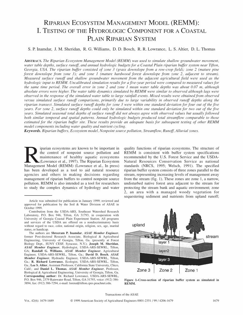
quality functions of riparian ecosystems. The structure ofREMM is consistent with buffer system specificationsrecommended by the U.S. Forest Service and the USDA-Natural Resources Conservation Service as nationalstandards (NRCS, 1995; Welsch, 1991). The specifiedriparian buffer system consists of three zones parallel to thestream, representing increasing levels of management awayfrom the stream (fig. 1). These zones are zone 1, a narrow,undisturbed native forest area adjacent to the stream forprotecting the stream bank and aquatic environment; zone2, an area with a managed woody vegetation forsequestering sediment and nutrients from upland runoff;

RIPARIAN ECOSYSTEM MANAGEMENT MODEL (REMM): I. TESTING OF THE HYDROLOGIC COMPONENT FOR A COASTAL

PLAIN RIPARIAN SYSTEM

S. P. Inamdar, J. M. Sheridan, R. G. Williams, D. D. Bosch, R. R. Lowrance, L. S. Altier, D. L. Thomas

ABSTRACT. The Riparian Ecosystem Management Model (REMM) was used to simulate shallow groundwater movement,water table depths, surface runoff, and annual hydrologic budgets for a Coastal Plain riparian buffer system near Tifton,Georgia, USA. The riparian buffer consisted of zone 3 (grass downslope from a row-crop field); zone 2 (mature pineforest downslope from zone 3); and zone 1 (mature hardwood forest downslope from zone 2, adjacent to stream).Measured surface runoff and shallow groundwater movement from the adjacent agricultural field were used as thehydrologic input to REMM. Uncalibrated simulation results for a five-year period were compared to measured values forthe same time period. The overall error in zone 2 and zone 1 mean water table depths was about 0.07 m, althoughabsolute errors were higher. The water table dynamics simulated by REMM were similar to observed although lags wereobserved in the response of the simulated water table to large rainfall events. Mixed results were obtained from observedversus simulated surface runoff comparisons, primarily due to large variability in observed runoff depths along theriparian transect. Simulated surface runoff depths for zone 3 were within one standard deviation for four out of the fiveyears. For zone 2, surface runoff depths could only be simulated within one standard deviation for two out of the fiveyears. Simulated seasonal total depths of surface runoff did not always agree with observed values but usually followedboth similar temporal and spatial patterns. Annual hydrologic budgets produced total streamflow comparable to thoseestimated for the riparian buffer site. These results provide an adequate basis for subsequent testing of other REMMmodel components including water quality and nutrient cycling.Keywords. Riparian buffers, Ecosystem model, Nonpoint source pollution, Streamflow, Runoff, Alluvial zones.

Article was submitted for publication in January 1999; reviewed andapproved for publication by the Soil & Water Division of ASAE inOctober 1999.

Contribution from the USDA-ARS, Southeast Watershed ResearchLaboratory, P.O. Box 946, Tifton, GA 31793, in cooperation withUniversity of Georgia Coastal Plain Experiment Station. All programsand services of the USDA are offered on a nondiscriminatory basiswithout regard to race, color, national origin, religion, sex, age, maritalstatus, or handicap.

The authors are Shreeram P. Inamdar, ASAE Member Engineer,former Post-doctoral Research Associate, Biological & AgriculturalEngineering, University of Georgia, Tifton, Ga. (presently at ForestBiology Dept., SUNY CESF, Syracuse, N.Y.); Joseph M. Sheridan,ASAE Member Engineer, Hydrologist, USDA-ARS-SEWRL, Tifton,GA; Randall G. Williams, ASAE Member Engineer, AgriculturalEngineer, USDA-ARS-SEWRL, Tifton, Ga.; David D. Bosch, ASAE

Member Engineer, Hydraulic Engineer, USDA-ARS-SEWRL, Tifton,Ga.; R. Richard Lowrance, Ecologist, USDA-ARS-SEWRL, Tifton,Ga.; Lee S. Altier, Assistant Professor, California State University, Chico,Calif.; and Daniel L. Thomas, ASAE Member Engineer, Professor,Biological & Agricultural Engineering, University of Georgia, Tifton, Ga.Corresponding author: Dr. Richard Lowrance, USDA-ARS-SEWRL,P.O. Box 946, 2379 Rainwater Road, Tifton, GA 31793, voice: (912) 386-3894, fax: (912) 386-7294, e-mail: [email protected].

Transactions of the ASAE

© 1999 American Society of Agricultural Engineers 0001-2351 / 99 / 4206-1679 1679VOL. 42(6): 1679-1689

Figure 1–Cross-section of riparian buffer system as simulated in

REMM.

and zone 3, an herbaceous filter strip for dispersal ofincoming upland surface runoff and sediment and nutrientdeposition. Although REMM is designed to simulate thistype of buffer system, the model can be used with othertypes of vegetation in a zone or with 1 to 3 zones.

Processes simulated in REMM include storage andmovement of surface and subsurface water, sedimenttransport and deposition, transport, sequestration, andcycling of nutrients, and vegetative growth. To simulateeach of these processes, REMM has four major modules:hydrology, sediment, nutrient, and vegetative growth.Simulations are performed on a daily basis and can becontinued in excess of 100 years. The intent of this articleis to provide a brief description and evaluation of theREMM hydrology component. This article is a companionarticle to a manuscript which evaluates the water qualityand nutrient cycling components of the model (Inamdar etal., 1999). In this article, we evaluate REMM bycomparing model simulations to field measured hydrologicdata from a riparian buffer site in the Gulf-Atlantic CoastalPlain near Tifton, Georgia, and to long-term hydrologicrecords from the Little River Watershed in the same area.

MODEL DESCRIPTIONIn REMM, the three zone buffer system has three soil

layers through which vertical and lateral movement ofwater and associated dissolved nutrients are simulated(fig. 1). The uppermost soil layer is covered by a litter layerwhich acts as a mixing layer and which interacts withsurface runoff. Water movement and storage ischaracterized by processes of interception, evapotrans-piration (ET), infiltration, vertical drainage, surface runoff,subsurface lateral flow, upward flux from the water table inresponse to ET, and exfiltration. These processes aresimulated for each of the three zones. The storage andmovement of water between the zones is based on acombination of mass balance and rate controlledapproaches. The mass balance of water within each soillayer is:

where θ[t] (mm) is the soil moisture on day t, θ[t – 1] (mm)is the soil moisture from the preceding day, QV-in (mm) isthe addition of water due to infiltration in case of the uppersoil layer, or drainage from upper soil layer forintermediate soil layers, QV-out (mm) is drainage out of thelayer, QH-in (mm) is contribution due to lateral subsurfaceflow, QH-out (mm) is the outflow of water to lateralsubsurface downslope flow, and ET (mm) is evapotrans-piration. Each of these processes is described briefly in thefollowing paragraphs. A more detailed discussion of themodel scope and structure is provided in Lowrance et al.(In Press) and Altier et al. (In Press).

Before precipitation reaches the soil surface, it is subjectto interception by plant canopies and surface litter. REMMsimulates two canopies at different heights above theground surface, each comprised of one or more plantspecies. Canopy interception is an exponential function of

the canopy storage capacity and the daily rainfall and issimulated using a modified form of the Thomas andBeasley (1986) equation and is given by:

where c is the canopy, s is the species type within a canopy,Int (mm) is intercepted moisture, Canfrac (ha ha–1) is thefraction of canopy occupied by the vegetation type, CSC(mm) is interception storage based on leaf area index, θLeaf(mm) is the intercepted rainfall depth on the leaf for thecurrent day, rain (mm) is rainfall depth, and PIT (mm) isthe potential canopy storage capacity for the species atmaximum leaf area index. Canopy storage capacity on anygiven day is a product of the leaf area index (LAI) on thatday and a species-specific storage capacity per unit LAI.Precipitation falling through the canopy (throughfall) issubjected to litter interception. Similar to canopyinterception, litter interception is determined by the depthof the litter at any given time and the litter storage capacity.

While intercepted water is available on the vegetativecanopy, evaporation of the intercepted water occurs.During this period all the radiant energy is used toevaporate the intercepted water. Transpiration proceedsafter all moisture on the canopy has been evaporated.Potential rate of leaf transpiration PT is computed using amodified form of the Penman Monteith equation (Runningand Coughlan, 1988):

where A is the net radiation energy (kJ–2 day–1), LAI(ha ha–1) is the canopy leaf area index on day t, λ is thelatent heat of vaporization (MJ Kg–1), ∆ is the slope of thesaturation vapor pressure curve (kPa °C–1), γ is thepsychrometric constant (kPa), ra is the aerodynamicresistance (s/m), ρa is the air density (kg m–3), D is thevapor pressure deficit (kPa), and cp is the specific heat ofair at constant pressure taken as 1.01 kJ kg–1 K–1, and rs isthe stomatal resistance. Leaf evaporation is also computedusing equation 3 except that for leaf evaporation thestomatal resistance term reduces to zero.

Potential transpiration for a plant type from equation 3is adjusted for the actual moisture available fortranspiration for that plant type. The amount of soilmoisture available for a plant type from a soil layerdepends on the proportion of its root within that layer andthe soil moisture content of the layer (eq. 4). Transpirationis allocated among the soil layers from the surfacedownward. The maximum rate of transpiration from a layeris limited by its hydraulic conductivity which varies withsoil moisture and is described by Campbell’s (1974)equation. This allows any excess demand that is notrealized by a layer to be transferred to the layer below.Transpiration by each plant type from a given soil layer is

PT c,s,t =LAI c,s,t

λ t

∆ t A c,s,t 10–3 +

ρa t cp D t

ra c,s,t

∆ t + λ t 1 +rs t

ra t

(3)

Int c,s,t = Canfrac c,s,t CSC c,s,t – θLeaf c,s,t

× 1 – exp – rain c,t CSC c,s,t

PIT s

2

(2)

θ t = θ t –1 + Q V-in t – Q V-out t

+ Q H-in t – Q H-out t – ET t (1)

1680 TRANSACTIONS OF THE ASAE

determined by multiplying available water by theproportion of total demand allocated for that plant type andsoil layer combination:

where, for soil layer j day t, AT is water uptake byvegetation s in canopy c from soil layer j (mm); K(θ) is soilhydraulic conductivity defined by Campbell’s equation forsoil layer j (mm); RPotTrans is remaining potentialtranspiration demand by vegetation s in canopy c from soillayer j after water has been taken up from the upper soillayers (mm); AdjMRF is a moisture factor adjusted for thefraction of the root mass of vegetation s from canopy c insoil layer j relative to its roots in the other layers andrelative to all other roots in layer j (0-1 scalar). θA isavailable water in soil layer j (mm):

where θWP is soil water content at wilting point (mm).Hence, for the first soil layer the transpiration demand for agiven plant type is equivalent to the total transpirationpotential of that plant type. In succeeding layers,RPotTrans is reduced by the sum of transpiration by allvegetation from upper layers:

The appropriate proportions of total water uptake demandare calculated as a function of a moisture factor adjustedfor root mass fractions:

where on day t, MRF is a moisture factor adjusted for thefraction of the root mass of vegetation s of canopy c inlayer j relative to its roots in the other layers (0-1 scalar);RFV is the fraction of the root mass of vegetation s incanopy c that is in soil layer j relative to all other roots in

layer j; MF is a moisture factor for layer j (0-1 scalar); andRFL is the fraction of the root mass of vegetation s incanopy c that is in soil layer j relative to its roots in theother layers.

The soil moisture factor (MF) represents the decreasingrate of transpiration that occurs as soil dries out. It wouldbe desirable to have this factor change during each day asET withdraws moisture from the soil layers, since itrepresents the influence of stomatal activity as well as ratesof moisture diffusion to the roots. However, with a dailytime step, it is calculated as a function of soil moisturestatus at the end of the previous day. The followingrelationship was used in the model as an approximation:

where θFC is soil moisture at field capacity (mm), and δ isa factor specific to the soil type that determines theinfluence of limiting soil water on ET.

Radiation energy filtering through the riparian canopyand reaching the litter surface is used to drive evaporationof litter moisture. Evaporation of litter moisture issimulated using procedures similar to that used forevaporation of intercepted water on leaf surfaces. Radiationenergy reaching the mineral soil surface (below the litterlayer) is the product of radiation at the litter surface and alitter transmission factor. Evaporation from the soil surfaceis computed according to the two stage process describedby Gardner and Hillel (1962).

Overland flow within the riparian zone can occur whensurface runoff from the upland field and/or contributionfrom throughfall exceeds the infiltration capacity of theriparian soil. Runoff depth from the upland field is a userinput. If the sum of incoming upland runoff and throughfalldepth is less than the infiltration capacity of the ripariansoil, water will infiltrate at the rate of application.However, during high intensity storms, the available watermay exceed the infiltration rate. In such conditions,infiltration is simulated using a modified form of theGreen-Ampt equation (Stone et al., 1994).

Since hydrologic computations are performed on a dailytime step, a detailed surface runoff routing scheme is notincluded. Field investigations though, show that surfacerunoff generated from fields during high intensity rainfallevents can have sufficient depth and velocity to traverse asignificant distance down the riparian slope beforeinfiltrating (Sheridan et al., 1996). This phenomenonbecomes especially significant in conditions where uplandrunoff enters the riparian zone as channelized orconcentrated flow. To account for this phenomena, a simplerouting scheme, limited only to upland runoff, wasintroduced. This scheme allows incoming upland runoff tobe distributed down the riparian slope based on its depthand flow velocity. The distributed depth is then summedwith throughfall for infiltration computations. The uplandrunoff routing procedure is developed assuming that runoffenters the riparian area as a rectangular slug with the lengthof the slug defined by the duration of flow and the volumeof the slug defined by the total runoff excess. The duration

MF j,t = Minimum of

1

θ t– 1 – θWP

δ θFC – θWP

(9)

MRF s,j,t = MF j,t × RFV s,j,t

MF j,t × RFV s,j,t∑j

3(8)

AdjMRF c,s,j,t = MRF c,s,j,t

× RFL c,s,j,t

∑c = 1

nMRF c,s,j,t × RFL c,s,j,t∑

s = 1

m(7)

RPotTrans c,s,j,t = PT c,s,t

RPotTrans c,s,j,t = PT c,s,t _ AT j,t∑i=1

j– 1

Layer 1

Layers 2, 3 (6)

θA j,t = 0

θA j,t = θ j,t – θWP

θ j,t < θWP

θWP ≤ θ j,t

(5)

AT c,s,j,t =

Min

K θ j,t

θA j,t × RPotTrans c,s,j,t × AdjMRF c,s,j,t

∑c = 1

nRPotTrans c,s,j,t × AdjMRF c,s,j,t∑

s = 1

m

(4)

1681VOL. 42(6): 1679-1689

of runoff is estimated as a function of the upslope drainagearea/field and is based on the equation developed byYoung et al. (1987). To determine the movement of theslug down the riparian zone the time of concentration forthe zone is computed as function of its Manningsroughness ‘n’ (Huggins and Burney, 1982). The distancethat upland surface runoff moves into the riparian zone isthen computed based on the upland runoff duration and thetime of concentration of the riparian zone.

Vertical drainage from a soil layer occurs when soilmoisture exceeds the field capacity. The amount drainedfrom a soil layer also depends on the capacity of thereceiving layer. The rate of drainage is set equal to thelesser of the hydraulic conductivities of the draining andreceiving layer. Unsaturated conductivity is simulated as afunction of the soil moisture content using Campbell’sequation (Campbell, 1974). In the presence of a shallowwater table, overlying soil layers are maintained at a higher(less negative) matric potential and consequently highersoil moisture contents. Assuming that the soil layer is inequilibrium with the water table, the matric potential at themid point of a soil layer can be determined by assumingthat the pressure head at that point is equal in magnitude tothe height of the point above the water table. The watercontent at this point is then determined using the moistureretention curve relating matric potential to the soil moisturecontent and described by Campbell’s equation.

In the presence of a shallow water table, a steadyupward flux will occur from the water table to the soillayer above to replenish ET from the layer. This upwardflux E at point p, a distance z above the water table, can bedescribed using the Darcy Buckingham equation given by(Skaggs, 1978):

where the h is the matric potential, z is the distance of thepoint from the water table (positive upwards), (∂h)/(∂z)expresses the gradient of matric potential, E is the upwardflux of water from the water table, and K(h) is theunsaturated hydraulic conductivity of the soil layerexpressed as a function of the matric potential h. Theequation is solved using a finite difference scheme similarto that used in DRAINMOD (Skaggs, 1978).

Subsurface lateral movement is assumed to occur whena water table builds up over the restricting soil layer. Thelateral movement of the water QH (mm) is simulated usingDarcy’s equation given by:

where Ks (mm day–1) is the saturated hydraulicconductivity, ∆h (m) is the difference in water surfacedepths between two zones, and L (m) is the horizontal flowdistance calculated as the distance between centers of twoadjacent zones. In the model, hydraulic conductivity isassumed to be isotropic. Downslope subsurface flowbetween the component zones is driven by the gradient ofthe water table. The potential hydraulic gradient that

determines subsurface movement from zone 1 to the streamis assumed equal to the smaller of the surface slope ofzone 1 and the gradient from the water table depth from themid point of zone 1 to the stream thalweg. Stream thalwegelevation is a user defined input. The model does notsimulate the influence of streamflow on the hydraulicgradient or the recharge of zone 1 from streamflow. Ifwater table intersects the land surface towards thedownslope edge of the riparian slope excess subsurfacewater is released to the surface as exfiltration. In addition,for a saturated soil profile, any excess throughfall orupslope surface runoff contributions will not infiltrate butare considered as saturation excess overland flow.

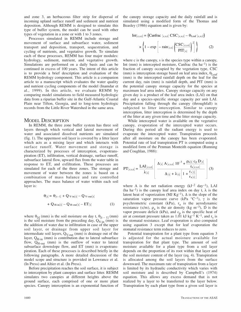
METHODSSITE DESCRIPTION AND DATA COLLECTION

Data for testing REMM was available fromexperimental riparian buffer sites located at the Universityof Georgia Gibbs Farm near Tifton, Georgia (Lowrance etal., 1998; Sheridan et al., 1996, 1999; Bosch et al., 1996).The study area is located in the Tifton Upland in thedrainage area of the Little River. The site has beenmanaged as a three-zone buffer system (fig. 2). While theriparian buffer is being maintained under three differenttreatments (Plots A, B, and C; fig. 2), only data from themature forest treatment (Plot A) was used for modelevaluation. In the description that follows, the dimension ofthe riparian buffer from the upland to the stream(or perpendicular to stream) is referred to as width, and thedistance along the stream is referred to as length. Thelength of the selected buffer treatment (Plot A) is 40.6 m.Zone 1 which is 15.2 m wide (area 0.06 ha), consists ofhardwoods, mostly yellow poplar (Liriodendron tulipiferaL.) and swamp black gum (Nyssa sylvatica var biflora

Q H t = Ks × ∆h t

L(11)

∂h

∂z = E

K h + 1 (10)


Figure 2–Layout of riparian zones, field boundaries, recording wells,

and runoff collection facilities at the Gibbs Farm site.

Marsh.). Zone 2 which is 50.3 m wide (area 0.20 ha),consists of conifers, primarily longleaf pine (Pinuspalustris Mill.) and slash pine (Pinus elliotti Engelm.).Zone 3 which is 7.6 m wide (area 0.03 ha), consists ofcommon Bermudagrass (Cynodon dactylon L. Pers.) andBahia grass (Paspalum notatum Flugge.) The contributingfield is 76.1 m wide (area 0.31 ha), yielding a field toriparian buffer ratio of 1:1. Most of the riparian area is anAlapaha loamy sand (loamy, siliceous, thermic ArenicPlinthic Paleaquults). The upland fields are Tifton loamysands (Calhoun, 1983).

Monitoring at this site was conducted from January1992 through December 1996. Data collected at this siteincluded (a) topographic and soil information; (b) weatherinformation; (c) surface runoff at the field-zone 3 interface,the zone 3-zone 2 interface, at the mid-point of zone 2, andat the zone 2-zone 1 interface (Sheridan et al., 1999); and(d) water table depths under the upland contributing fieldand each of the three component zones of the riparianbuffer (Bosch et al., 1996).

MODEL PARAMETERIZATION AND INITIALIZATION

With respect to hydrology, the information required bythe model includes daily weather data, daily surface andsubsurface runoff loading from the contributing field, andparameter values representing the topographic, soil, andvegetative conditions within the riparian buffer. Dailyweather data collected at the Gibbs farm site includedrainfall amount (mm), rainfall duration (h), maximum airtemperature (°C), minimum temperature (°C), solarradiation (langley’s day–1), wind speed (ms–1), and dewpoint temperature (°C). Runoff collected by surface runoffsamplers at the field-zone 3 interface was used to generatethe daily surface runoff depth (mm per unit contributingarea) input to REMM (Sheridan et al., 1999). Dailysubsurface flow loading to the buffer (mm per unitcontributing area) was computed using the hydraulicgradient between upland wells P3 and P4 (fig. 2) andrecording well 01 in zone 3, saturated thickness at well 01,and saturated hydraulic conductivity of 48 mm h–1 (Boschet al., 1996). Parameters that describe the riparian bufferdimensions, soil, and vegetation characteristics werederived from currently measured data and previouslypublished literature for the Gibbs farm site (Bosch et al.,1996; Perkins et al., 1986; Sheridan et al, 1996). A listing

of selected parameters and the corresponding values used isprovided in table 1. Values used to describe the topography,soil, and vegetation were best estimates based on measureddata and were not adjusted or calibrated during evaluationruns.

To evaluate model performance, simulated water tabledepths and surface runoff were compared to those observedat the experimental site. Water table comparisons werebased on daily recordings of wells in zones 2 and 1.Comparisons between model simulated and observed watertables for zone 3 were not performed because: (a) watertable depths in zone 3 along with upland well depths wereused to generate subsurface water input to the riparianzone; and (b) for long periods during summer and fallwater table depths in zone 3 dropped below the screenedwell depth (approximately 1.8 m from the surface) andwere unavailable. When zone 3 water table dropped belowthe screened depth subsurface water input to the riparianzone was computed by assuming the water table depth inzone 3 to be at the screened depth. It is possible that thisassumption resulted in a slightly higher subsurface waterinput from the field to the riparian zone. Surface runoffcomparisons were made on both an annual and seasonalbasis for positions corresponding to surface runoffcollectors at the zone 3-zone 2 interface and the zone 2-zone 1 interface. A general evaluation of the model wasconducted by developing annual hydrologic budgets forsimulated results and comparing these budget values withdata from the Little River Watershed, which contains theriparian buffer test site.

RESULTS AND DISCUSSIONWATER TABLE COMPARISONS

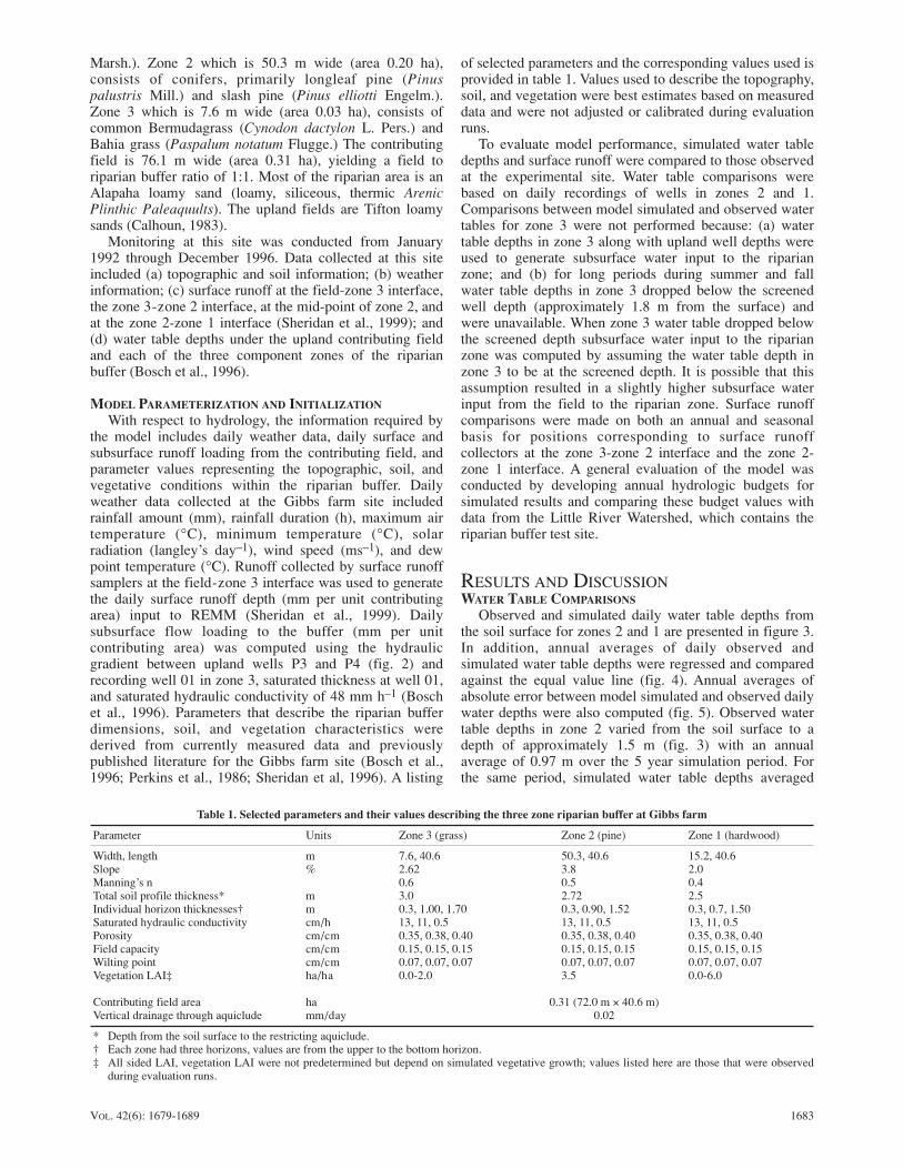
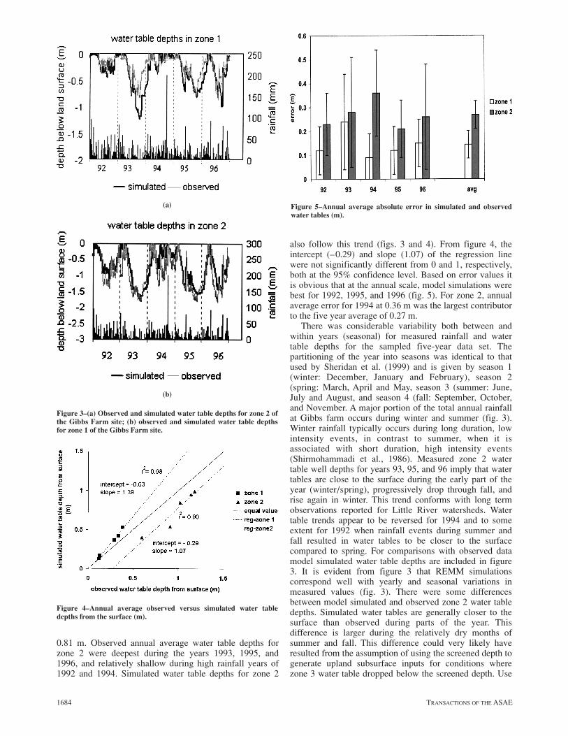
Observed and simulated daily water table depths fromthe soil surface for zones 2 and 1 are presented in figure 3.In addition, annual averages of daily observed andsimulated water table depths were regressed and comparedagainst the equal value line (fig. 4). Annual averages ofabsolute error between model simulated and observed dailywater depths were also computed (fig. 5). Observed watertable depths in zone 2 varied from the soil surface to adepth of approximately 1.5 m (fig. 3) with an annualaverage of 0.97 m over the 5 year simulation period. Forthe same period, simulated water table depths averaged

1683VOL. 42(6): 1679-1689

Table 1. Selected parameters and their values describing the three zone riparian buffer at Gibbs farm

Parameter Units Zone 3 (grass) Zone 2 (pine) Zone 1 (hardwood)

Width, length m 7.6, 40.6 50.3, 40.6 15.2, 40.6Slope % 2.62 3.8 2.0Manning’s n 0.6 0.5 0.4Total soil profile thickness* m 3.0 2.72 2.5Individual horizon thicknesses† m 0.3, 1.00, 1.70 0.3, 0.90, 1.52 0.3, 0.7, 1.50Saturated hydraulic conductivity cm/h 13, 11, 0.5 13, 11, 0.5 13, 11, 0.5Porosity cm/cm 0.35, 0.38, 0.40 0.35, 0.38, 0.40 0.35, 0.38, 0.40Field capacity cm/cm 0.15, 0.15, 0.15 0.15, 0.15, 0.15 0.15, 0.15, 0.15Wilting point cm/cm 0.07, 0.07, 0.07 0.07, 0.07, 0.07 0.07, 0.07, 0.07Vegetation LAI‡ ha/ha 0.0-2.0 3.5 0.0-6.0

Contributing field area ha 0.31 (72.0 m × 40.6 m)Vertical drainage through aquiclude mm/day 0.02

* Depth from the soil surface to the restricting aquiclude.† Each zone had three horizons, values are from the upper to the bottom horizon.‡ All sided LAI, vegetation LAI were not predetermined but depend on simulated vegetative growth; values listed here are those that were observed

during evaluation runs.

0.81 m. Observed annual average water table depths forzone 2 were deepest during the years 1993, 1995, and1996, and relatively shallow during high rainfall years of1992 and 1994. Simulated water table depths for zone 2

also follow this trend (figs. 3 and 4). From figure 4, theintercept (–0.29) and slope (1.07) of the regression linewere not significantly different from 0 and 1, respectively,both at the 95% confidence level. Based on error values itis obvious that at the annual scale, model simulations werebest for 1992, 1995, and 1996 (fig. 5). For zone 2, annualaverage error for 1994 at 0.36 m was the largest contributorto the five year average of 0.27 m.

There was considerable variability both between andwithin years (seasonal) for measured rainfall and watertable depths for the sampled five-year data set. Thepartitioning of the year into seasons was identical to thatused by Sheridan et al. (1999) and is given by season 1(winter: December, January and February), season 2(spring: March, April and May, season 3 (summer: June,July and August, and season 4 (fall: September, October,and November. A major portion of the total annual rainfallat Gibbs farm occurs during winter and summer (fig. 3).Winter rainfall typically occurs during long duration, lowintensity events, in contrast to summer, when it isassociated with short duration, high intensity events(Shirmohammadi et al., 1986). Measured zone 2 watertable well depths for years 93, 95, and 96 imply that watertables are close to the surface during the early part of theyear (winter/spring), progressively drop through fall, andrise again in winter. This trend conforms with long termobservations reported for Little River watersheds. Watertable trends appear to be reversed for 1994 and to someextent for 1992 when rainfall events during summer andfall resulted in water tables to be closer to the surfacecompared to spring. For comparisons with observed datamodel simulated water table depths are included in figure3. It is evident from figure 3 that REMM simulationscorrespond well with yearly and seasonal variations inmeasured values (fig. 3). There were some differencesbetween model simulated and observed zone 2 water tabledepths. Simulated water tables are generally closer to thesurface than observed during parts of the year. Thisdifference is larger during the relatively dry months ofsummer and fall. This difference could very likely haveresulted from the assumption of using the screened depth togenerate upland subsurface inputs for conditions wherezone 3 water table dropped below the screened depth. Use


Figure 3–(a) Observed and simulated water table depths for zone 2 of

the Gibbs Farm site; (b) observed and simulated water table depths

for zone 1 of the Gibbs Farm site.

(b)

(a)

Figure 4–Annual average observed versus simulated water table

depths from the surface (m).

Figure 5–Annual average absolute error in simulated and observed

water tables (m).

of this assumption will overestimate the upland subsurfaceflow contributions. Observed water tables appear to reachtheir maximum depths in early fall (September to October)and start rising by late fall (November). Simulated depthsalso reach maximum depth by early fall but do not respondto rainfall as quickly as the observed values (especially for1993 and 1995).

At the annual scale, zone 1 water tables were bestsimulated by the model, which is supported by both visualcomparisons (fig. 3) and small annual average errorbetween observed and simulated daily water table depths(fig. 5). The intercept (–0.03) and slope (1.39) of theregression line (fig. 4) were also not significantly differentfrom 0 and 1 respectively, at the 95% confidence level.Zone 1 was considerably wetter than zones 2 and 3throughout the year with observed water table depthsvarying from the surface to approximately 0.40 m belowthe surface. Similar to zone 2, the largest drops in thezone 1 water tables were observed during 1993, 1995, and1996 (fig. 3). Model simulations followed this trend.Although simulated water table depths were in error by0.14 m over the five-year period (fig. 5), there was a mixedtrend with respect to individual years, with error betweensimulated and observed being least for the wettest year(1994) followed by the driest year (1995).

In contrast to zone 2, where simulated water tables werecloser to the surface than observed during summer and fall,simulated zone 1 depths were slightly lower than observed.This indicates that water loss during summer and fall wasoverestimated by the model. Zone 1 provides shallowgroundwater discharge to streamflow. Field observations atthe Gibbs Farm site and elsewhere in Little Riverwatershed show that streamflow occurs typically duringwinter, early spring, and late summer. Winter streamflowsare generated by lateral subsurface flow, exfiltration, andsurface runoff from saturated alluvial soils within zone 1(Shirmohammadi et al., 1986). Late summer flows areprimarily supported by infiltration excess surface runoffassociated with high intensity rainfall events. Siteobservations during winter at the Gibbs Farm riparian siteindicated that streamflow from upstream areas is alsoentering throughout the length of the riparian buffer underconsideration. Flows from upstream might cause runoffgenerated within zone 1 to “back up” and cause localflooding within zone 1. This “backing up” of zone 1 wateressentially leads to elevated water tables within zone 1during this period. The influences of streamflow on zone 1water tables are not currently included in REMM. Thisphenomenon (streamflow influences) is proposed forinclusion in the next version of REMM. Absence ofstreamflow influences in the current version of REMM is alikely reason for lower simulated (than observed) watertables in zone 1 during the year. This same phenomenacould explain sudden increases in observed zone 1 watertables during summer, which is not reproduced in modelsimulations to the extent observed. Flows from upstreamareas associated with high intensity rainfall events duringsummer could cause water table increases in the near-stream zone 1. In addition to errors caused by streamflowinfluences, it is also possible that the model might beoverestimating ET during summer for zone 1. Overall,model simulated water table depths are good consideringthat soil parameters used in the model were based on best

literature and measured estimates and were not calibrated,and phenomenon such as streamflow influence on riparianwater tables are not currently simulated.

SURFACE RUNOFF COMPARISONS

Observed and simulated annual totals of surface runoffexiting zones 3 and 2 are presented in figure 6. Althoughmeasured and model comparisons were limited to runoffexiting the zones, values for runoff measured at the middleof zone 2 were also included in figure 6 to highlight thevariability in runoff along the riparian transect. Surfacerunoff exiting zone 1 could not be measured due todifficulties in sampling surface runoff immediatelyadjacent to the edge of an intermittent stream. However,simulated runoff values exiting zone 1 are included infigure 6. In addition to annual runoff totals, observed andsimulated average annual surface runoff event depthsexiting zones 2 and 3 are presented in figure 7. Prior tocomparing these results it is important to point out that thesurface runoff collectors used at this site are designed suchthat they are best suited for conditions where surface runoffis uniformly distributed spatially over the soil surface(Sheridan et al., 1996). If runoff concentration occurs, andif concentrated flow bypasses the collectors, the runoffmeasured by the collectors might not be representative ofthe actual field conditions. Surface runoff depths (values infigs. 6 and 7) at a point along the riparian transect(either exiting a zone or at the mid point of the zone) werecomputed by dividing the total runoff volume collected atthat point by the contributing area upslope of that point.

Measured annual surface runoff loadings from the field(which were also used directly as input to the model)varied significantly over the five-year period ranging froma high of 317 mm to a low of 22 mm and averaging150 mm (fig. 6). Observed runoff from the field did notappear to show strong correspondence with annual rainfalltotals. For instance, runoff for 1995 (109 mm) wasgenerated by annual rainfall of 877 mm while runoff for1993 (22 mm) occurred with substantially higher rainfall(1100 mm) (table 3). The timing of rainfall was clearlyimportant for observed surface runoff. Surface runoff wasthe second largest source of water to the riparian zone, withsubsurface input being one third of the surface total (table3). Measured surface runoff totals presented in figure 6reveal an unexpected and interesting trend. For all years,surface runoff from the field is always greater than runoffat any other location along the field-riparian transect (fig.6). This field runoff is reduced considerably as it passesthrough the grassed zone 3, which is as expected. Runoffexiting zone 2 is less than that exiting zone 3, which tendsto suggest that field runoff is lost to infiltration as it travelsfurther downslope into the riparian zone. However, runoffrecorded at the mid point of zone 2 appears to disagreewith this trend. Runoff depths recorded at the mid point ofzone 2 appear to be greater than or nearly equal to thoserecorded at the downslope edge of zone 3, and alwaysgreater than those recorded at the downslope edge of zone2. These high surface runoff depths at the middle of thezone 2 cannot be explained. It is likely that these highvalues could have been a result of the limitation of thesample collectors. It is possible that runoff concentrationinto one of the surface collectors at the middle of the zone2 could have resulted in more runoff collection at this

1685VOL. 42(6): 1679-1689

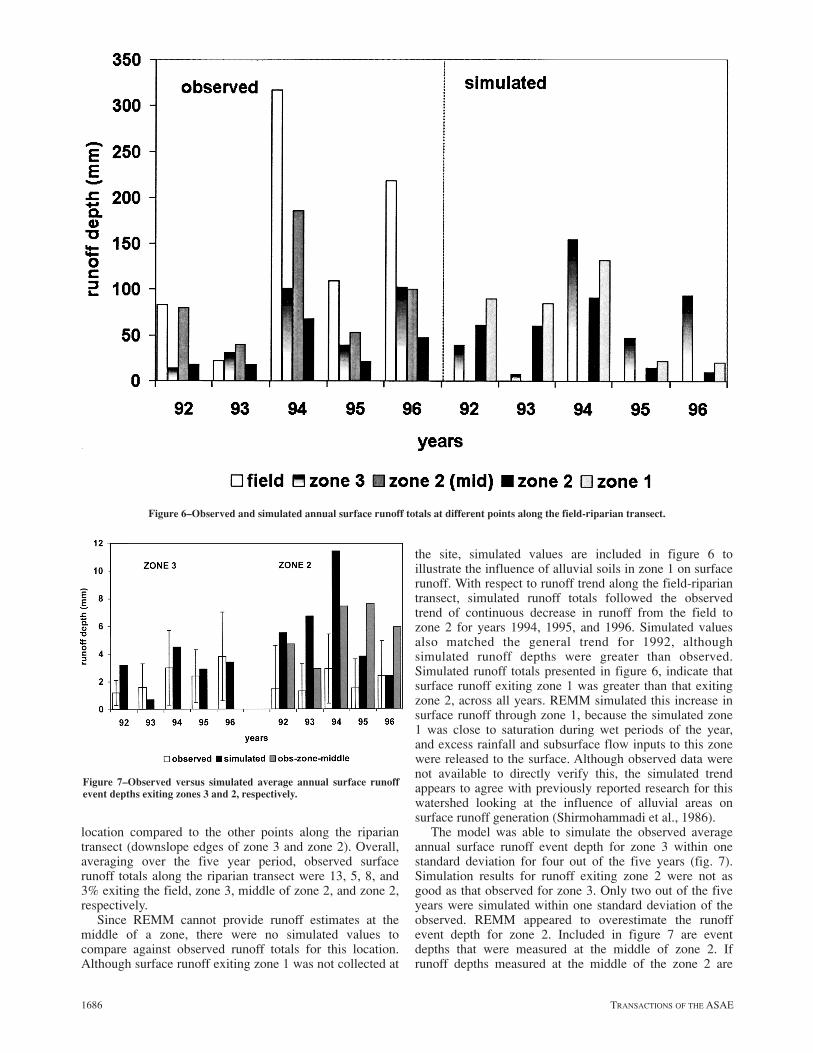
location compared to the other points along the ripariantransect (downslope edges of zone 3 and zone 2). Overall,averaging over the five year period, observed surfacerunoff totals along the riparian transect were 13, 5, 8, and3% exiting the field, zone 3, middle of zone 2, and zone 2,respectively.

Since REMM cannot provide runoff estimates at themiddle of a zone, there were no simulated values tocompare against observed runoff totals for this location.Although surface runoff exiting zone 1 was not collected at

the site, simulated values are included in figure 6 toillustrate the influence of alluvial soils in zone 1 on surfacerunoff. With respect to runoff trend along the field-ripariantransect, simulated runoff totals followed the observedtrend of continuous decrease in runoff from the field tozone 2 for years 1994, 1995, and 1996. Simulated valuesalso matched the general trend for 1992, althoughsimulated runoff depths were greater than observed.Simulated runoff totals presented in figure 6, indicate thatsurface runoff exiting zone 1 was greater than that exitingzone 2, across all years. REMM simulated this increase insurface runoff through zone 1, because the simulated zone1 was close to saturation during wet periods of the year,and excess rainfall and subsurface flow inputs to this zonewere released to the surface. Although observed data werenot available to directly verify this, the simulated trendappears to agree with previously reported research for thiswatershed looking at the influence of alluvial areas onsurface runoff generation (Shirmohammadi et al., 1986).

The model was able to simulate the observed averageannual surface runoff event depth for zone 3 within onestandard deviation for four out of the five years (fig. 7).Simulation results for runoff exiting zone 2 were not asgood as that observed for zone 3. Only two out of the fiveyears were simulated within one standard deviation of theobserved. REMM appeared to overestimate the runoffevent depth for zone 2. Included in figure 7 are eventdepths that were measured at the middle of zone 2. Ifrunoff depths measured at the middle of the zone 2 are


Figure 6–Observed and simulated annual surface runoff totals at different points along the field-riparian transect.

Figure 7–Observed versus simulated average annual surface runoff

event depths exiting zones 3 and 2, respectively.

included in the comparisons, simulated runoff depthsexiting zone 2, especially for years 1995 and 1996, appearto fall within the values measured at the middle of zone 2and those exiting zone 2.

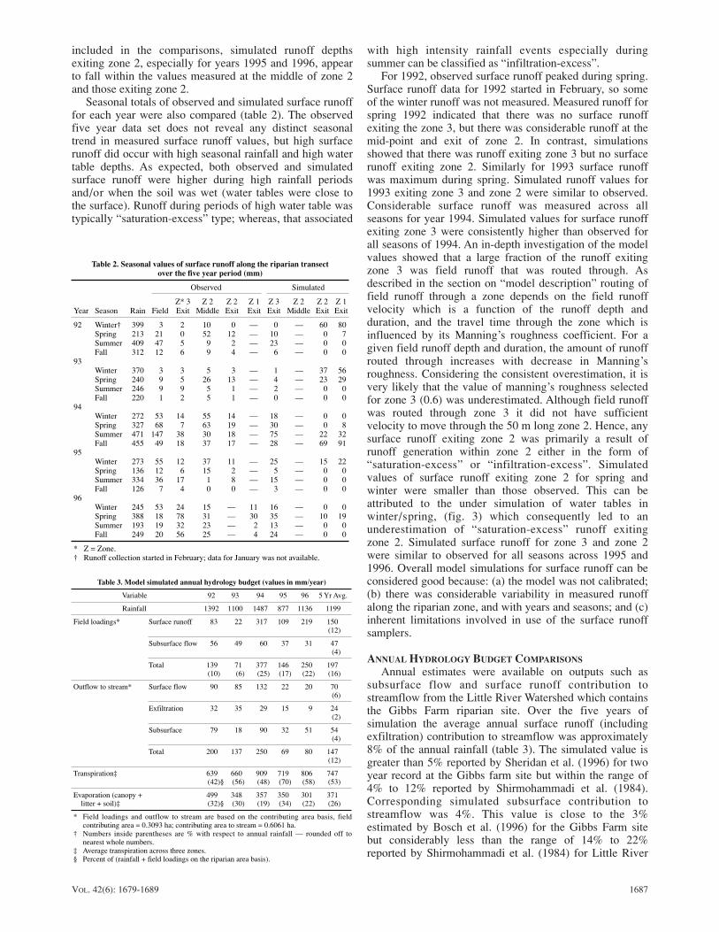
Seasonal totals of observed and simulated surface runofffor each year were also compared (table 2). The observedfive year data set does not reveal any distinct seasonaltrend in measured surface runoff values, but high surfacerunoff did occur with high seasonal rainfall and high watertable depths. As expected, both observed and simulatedsurface runoff were higher during high rainfall periodsand/or when the soil was wet (water tables were close tothe surface). Runoff during periods of high water table wastypically “saturation-excess” type; whereas, that associated

with high intensity rainfall events especially duringsummer can be classified as “infiltration-excess”.

For 1992, observed surface runoff peaked during spring.Surface runoff data for 1992 started in February, so someof the winter runoff was not measured. Measured runoff forspring 1992 indicated that there was no surface runoffexiting the zone 3, but there was considerable runoff at themid-point and exit of zone 2. In contrast, simulationsshowed that there was runoff exiting zone 3 but no surfacerunoff exiting zone 2. Similarly for 1993 surface runoffwas maximum during spring. Simulated runoff values for1993 exiting zone 3 and zone 2 were similar to observed.Considerable surface runoff was measured across allseasons for year 1994. Simulated values for surface runoffexiting zone 3 were consistently higher than observed forall seasons of 1994. An in-depth investigation of the modelvalues showed that a large fraction of the runoff exitingzone 3 was field runoff that was routed through. Asdescribed in the section on “model description” routing offield runoff through a zone depends on the field runoffvelocity which is a function of the runoff depth andduration, and the travel time through the zone which isinfluenced by its Manning’s roughness coefficient. For agiven field runoff depth and duration, the amount of runoffrouted through increases with decrease in Manning’sroughness. Considering the consistent overestimation, it isvery likely that the value of manning’s roughness selectedfor zone 3 (0.6) was underestimated. Although field runoffwas routed through zone 3 it did not have sufficientvelocity to move through the 50 m long zone 2. Hence, anysurface runoff exiting zone 2 was primarily a result ofrunoff generation within zone 2 either in the form of“saturation-excess” or “infiltration-excess”. Simulatedvalues of surface runoff exiting zone 2 for spring andwinter were smaller than those observed. This can beattributed to the under simulation of water tables inwinter/spring, (fig. 3) which consequently led to anunderestimation of “saturation-excess” runoff exitingzone 2. Simulated surface runoff for zone 3 and zone 2were similar to observed for all seasons across 1995 and1996. Overall model simulations for surface runoff can beconsidered good because: (a) the model was not calibrated;(b) there was considerable variability in measured runoffalong the riparian zone, and with years and seasons; and (c)inherent limitations involved in use of the surface runoffsamplers.

ANNUAL HYDROLOGY BUDGET COMPARISONS

Annual estimates were available on outputs such assubsurface flow and surface runoff contribution tostreamflow from the Little River Watershed which containsthe Gibbs Farm riparian site. Over the five years ofsimulation the average annual surface runoff (includingexfiltration) contribution to streamflow was approximately8% of the annual rainfall (table 3). The simulated value isgreater than 5% reported by Sheridan et al. (1996) for twoyear record at the Gibbs farm site but within the range of4% to 12% reported by Shirmohammadi et al. (1984).Corresponding simulated subsurface contribution tostreamflow was 4%. This value is close to the 3%estimated by Bosch et al. (1996) for the Gibbs Farm sitebut considerably less than the range of 14% to 22%reported by Shirmohammadi et al. (1984) for Little River

1687VOL. 42(6): 1679-1689

Table 2. Seasonal values of surface runoff along the riparian transect

over the five year period (mm)

Observed Simulated

Z* 3 Z 2 Z 2 Z 1 Z 3 Z 2 Z 2 Z 1Year Season Rain Field Exit Middle Exit Exit Exit Middle Exit Exit

92 Winter† 399 3 2 10 0 — 0 — 60 80Spring 213 21 0 52 12 — 10 — 0 7Summer 409 47 5 9 2 — 23 — 0 0Fall 312 12 6 9 4 — 6 — 0 0

93Winter 370 3 3 5 3 — 1 — 37 56Spring 240 9 5 26 13 — 4 — 23 29Summer 246 9 9 5 1 — 2 — 0 0Fall 220 1 2 5 1 — 0 — 0 0



96Winter 245 53 24 15 — 11 16 — 0 0Spring 388 18 78 31 — 30 35 — 10 19Summer 193 19 32 23 — 2 13 — 0 0Fall 249 20 56 25 — 4 24 — 0 0

* Z = Zone.† Runoff collection started in February; data for January was not available.

Table 3. Model simulated annual hydrology budget (values in mm/year)

Variable 92 93 94 95 96 5 Yr Avg.

Rainfall 1392 1100 1487 877 1136 1199

Field loadings* Surface runoff 83 22 317 109 219 150(12)

Subsurface flow 56 49 60 37 31 47(4)

Total 139 71 377 146 250 197(10) (6) (25) (17) (22) (16)

Outflow to stream* Surface flow 90 85 132 22 20 70(6)

Exfiltration 32 35 29 15 9 24(2)

Subsurface 79 18 90 32 51 54(4)

Total 200 137 250 69 80 147(12)

Transpiration‡ 639 660 909 719 806 747(42)§ (56) (48) (70) (58) (53)

Evaporation (canopy + 499 348 357 350 301 371litter + soil)‡ (32)§ (30) (19) (34) (22) (26)

* Field loadings and outflow to stream are based on the contributing area basis, fieldcontributing area = 0.3093 ha; contributing area to stream = 0.6061 ha.

† Numbers inside parentheses are % with respect to annual rainfall — rounded off tonearest whole numbers.

‡ Average transpiration across three zones.§ Percent of (rainfall + field loadings on the riparian area basis).

watershed. The five-year average also showed that surfacerunoff decreased as a proportion of the rainfall from thefield through the riparian buffer (from 12% to 8%; table 3);whereas, subsurface flow remained steady around 4%.Total streamflow from the Gibbs Farm site averaged147 mm, or about 40% of the long-term average for LittleRiver Watershed (370 mm, Sheridan, 1997).

The hydrologic budget estimates presented in table 3also provide a salient result, that upland loadings to thebuffer may not necessarily determine the magnitude ofsurface and subsurface runoff that is generated within thebuffer and which eventually contribute to streamflow. Thisis obvious from budgets of years 1993 and 1996, whereeven though field loadings for 1993 were much smallerthan those of 1996, streamflow contribution was higher in1993 compared to that of 1996. A closer look at the budgetsreveals that surface runoff contribution to streamflowduring 1993 was more than twice that of 1996. A plot ofthe monthly rainfall, water table, and surface runoffgenerated for zone 1 for 1993 and 1996 (not included heredue to space limitations) revealed that most of the surfacerunoff which contributed to streamflow in 1993 wasgenerated during winter/early spring (table 2). There werea number of large rainfall events during winter and earlyspring of 1993 when the soil in zone 1 was alreadysaturated and which resulted in saturation excess surfacerunoff. Compared to 1993, 1996 had less rainfall during theearly part of the year and water tables were much deepercompared to 1993 (fig. 3). This analysis indicates that inaddition to upland loadings, the amount of rainfall, itsdistribution during the year, and the soil moistureconditions in the alluvial zone (zone 1 in this case) are animportant determinant of streamflow. This result isconsistent with conclusions of Shirmohammadi et al.(1986) who found that generation of streamflow on LittleRiver Watershed was largely controlled by soil moistureconditions in the alluvial aquifer of the riparian zone.

Simulated transpiration of 747 mm yr–1 averaged overfive years and across the three vegetation types (table 3) isin the neighborhood of values reported in literature forsimilar site conditions (Riekerk, 1985; Ewel and Smith,1992). ET for the riparian zone at 79% of the effectiverainfall (sum of rainfall + upland field loadings) is in theneighborhood of estimates of ET for Little River Watershed(Sheridan, 1997).

SUMMARY AND CONCLUSIONSThe five year simulations of the Gibbs Farm site reflect

many of the dynamics of the observed data. Theuncalibrated simulations respond in expected fashion todifferences in annual and seasonal patterns of precipitation.In general, simulated water tables were higher thanobserved in zone 2 and lower than observed in zone 1.Lower water tables in zone 1 seem to be related to the factthat REMM does not account for overbank flooding andthe influence of streamflow on water table conditions. Theabsolute water table depth error was 0.27 m and 0.14 m forzones 2 and 1, respectively. These differences do not reflectthat simulated can be either higher or lower than observed.The actual mean water table depth for simulated andobserved only differ by 0.07 m for the mean of zone 2 andzone 1 combined. This is a very small difference

considering that the model was not calibrated. Outputs tothe stream are controlled by hydrologic conditions inzone 1. The smaller difference in simulated and observedwater table conditions in zone 1 seem to be a goodapproximation of the water table conditions controllingsubsurface output to the stream, especially when overbankflooding is minor.

Simulated surface runoff depths show similar patterns tothe observed runoff. Average annual event runoff depthsexiting zone 3 were simulated within one standarddeviation of the observed for four out of the five years.Corresponding simulated runoff depths for zone 2 weregreater than the observed and only two out of the five yearswere within one standard deviation of the observed.Although observed surface runoff outputs from zone 1were not available, REMM simulated higher per ha runofffrom zone 1 than zone 2. This result is consistent with fieldobservations and earlier studies of the impact of alluvialareas on streamflow generation in this type of coastal plainwatershed.

The overall hydrologic budgets for the riparianecosystem are similar to independent estimates ofsubsurface flow at the site (Bosch et al., 1996). Thebudgets differ from larger scale water budgets for LittleRiver watershed. The Gibbs Farm site is more dominatedby surface runoff than subsurface flow, in contrast to othersites studied in the region. The amount of streamflowgenerated by the model is lower than watershed scaleestimates but reflect the low estimated loadings from theupland field (197 mm). The uncalibrated simulationsindicate that ET is nearly equal to the long-term watershedscale estimates.

Calibration of components of the water balance couldyield estimates of streamflow which better match long-term watershed averages. This could be done by calibratingsimulated ET. Yet, given the relatively small field input tothe riparian zone simulated with REMM, the hydrologysimulation results reflect the conditions provided forREMM; discharge is probably less than measured on largerwatersheds. Given the close agreement between averagewater table depths, water table patterns, surface runoffvolumes, and patterns of surface runoff, the uncalibratedhydrology simulations provide an adequate basis for thewater quality and nutrient cycling evaluations to follow(Inamdar et al., 1999).

REFERENCESAltier, L. S., R. R. Lowrance, R. G. Williams, S. P. Inamdar, D. D.

Bosch, J. M. Sheridan, R. K. Hubbard, and D. L. Thomas.1999. Riparian Ecosystem Management Model (REMM):Documentation. USDA Conservation Research Report (InPress).

Bosch, D. D., J. M. Sheridan, and R. R. Lowrance. 1996.Hydraulic gradients and flow rates of a shallow coastal plainaquifer in a forested riparian buffer. Transactions of the ASAE39(3): 865-871.

Calhoun, J. W. 1983. Soil Survey of Tift County, Georgia.Washington, D.C: USDA-SCS.

Campbell, G. S. 1974. A simple method for determiningunsaturated conductivity from moisture retention data. Soil Sci.117: 311-314.

Ewel, K. C., and J. E. Smith. 1992. Evapotranspiration fromFlorida Cypress swamps. Water Res. Bull. 28(2): 299-304.


Gardner, W. R., and D. I. Hillel. 1962. The relation of externalevaporative conditions to the drying of soils. J. Geophys. Res.67: 4319-4325.

Huggins, L. F., and J. R. Burney. 1982. Surface runoff, storage,and routing. In Hydrologic Modeling of Small Watersheds, eds.C. T. Haan, H. P. Johnson, and D. L. Brakensiek. St. Joseph,Mich.: ASAE.

Inamdar, S. P., R. R. Lowrance, L. S. Altier, R. G. Williams, and R.K. Hubbard. Riparian Ecosystem Management Model(REMM): II. Testing of the water quality and nutrient cyclingcomponents for a Coastal Plain riparian system. Transactionsof the ASAE 42(6): 1691-1707.

Lowrance, R. R. 1981. Nutrient cycling in an agriculturalwatershed: Waterborne nutrient input/output budgets for theriparian zone. Unpub. Ph.D. diss. Athens, Ga.: University ofGeorgia.

Lowrance, R. R., L. S. Altier, R. G. Williams, S. P. Inamdar, J. M.Sheridan, D. D. Bosch, R. K. Hubbard, and D. L. Thomas.2000. REMM: The Riparian Ecosystem Management Model. J.Soil & Water Conserv. (In Press).

Lowrance, R. R., L. S. Altier, R. G. Williams, S. P. Inamdar, D. D.Bosch, J. M. Sheridan, and D. L. Thomas. 1998. The RiparianEcosystem Management Model (REMM): Simulator forecological processes in buffer systems. In Proc. First FederalInteragency Hydrologic Modeling Conference, 1-81 to 1-88Las Vegas, Nev. Reston, Va.: USGS.

Lowrance, R. R., L. S. Altier, J. D. Newbold, R. R. Schnabel, P. M.Groffman, J. M. Denver, D. L. Correll, J. W. Gilliam, J. L.Robinson, R. B. Brinsfield, K. W. Staver, W. C. Lucas, and A.H. Todd. 1997. Water quality functions of riparian forest buffersystems in the Chesapeake Bay watersheds. Environ. Manage.21(5): 687-712.

NRCS. 1995. Riparian Forest Buffer, 392. Seattle, Wash.: NRCSWatershed Science Institute.

Perkins, H. F., J. E. Hook, and N. W. Barbour. 1986. SoilCharacteristics of Selected Areas of the Coastal PlainExperiment Station and ABAC Research Farms. GeorgiaAgricultural Experiment Stations, University of Georgia. Res.Bull. 346.

Riekerk, H. 1985. Lysimetric measurement of pineevapotranspiration for water balances. In Advances inEvapotranspiration, 276-281. St. Joseph, Mich.: ASAE.

Running, S. W., and J. C. Coughlan. 1988. A general model offorest ecosystem processes for regional applications I.Hydrologic balance, canopy gas exchange and primaryproduction processes. Ecol. Model. 42: 125-154.

Sheridan, J. M. 1997. Rainfall-streamflow relations for CoastalPlain watersheds. Applied Engineering in Agriculture 13(3):333-344.

Sheridan, J. M., R. R. Lowrance, and D. D. Bosch. 1999.Management effects on runoff and sediment transport inriparian forest buffers. Transactions of the ASAE 42(1): 55-64.

Sheridan, J. M., R. R. Lowrance, and H. H. Henry. 1996. Surfaceflow sampler for riparian studies. Applied Engineering inAgriculture 12(2): 183-188.

Shirmohammadi, A. J., J. M. Sheridan, and L. E. Asmussen. 1986.Hydrology of alluvial stream channels in southern CoastalPlain watersheds. Transactions of the ASAE 29(1): 135-142.

Shirmohammadi, A. J., J. M. Sheridan, and W. G. Knisel. 1984. Anapproximate method for partitioning daily streamflow data. J.Hydrol. 74(3/4): 335-354.

Skaggs, R. W. 1978. A water management model for shallow watertable soils. WRRI, University of North Carolina Report No.134.

Stone, J. J., R. H. Hawkins, and E. D. Shirley. 1994. Anapproximate form of the Green Ampt infiltration equation.ASCE J. Irrig. & Drain. 120(1): 128-137.

Thomas, D. L., and D. B. Beasley. 1986. A physically based foresthydrology model I: Development and sensitivity ofcomponents. Transactions of the ASAE 29(4): 962-972.

Welsch, D. J. 1991. Riparian Forest Buffers. USDA-FS Publ. No.NA-PR-07-91. Radnor, Pa.: USDA.

Young, R. A., C. A. Onstad, D. D. Bosch, and W. P. Anderson.1987. AGNPS: Agricultural Non-Point Source PollutionModel. USDA, Conservation Research Report 35. Washington,D.C.: USDA.

1689VOL. 42(6): 1679-1689

Documents

RIPARIAN ECOSYSTEM MANAGEMENT MODEL … Inamdar TASAE 42(6) Riparian... · The overall error in zone 2 and zone 1 mean water table depths was about 0.07 ... 3894, fax: (912) 386-7294,