Ed

BZa

b

c

d

e

a

ARRAA

KREWPB

1

retoimpwdeus

h1

Ecological Indicators 69 (2016) 873–881

Contents lists available at ScienceDirect

Ecological Indicators

j o ur na l ho me page: www.elsev ier .com/ locate /eco l ind

valuation of ecosystem service value of riparian zone using land useata from 1986 to 2012

olin Fua,b,c, Ying Lia,∗, Yeqiao Wangc, Bai Zhanga, Shubai Yind, Honglei Zhue,efeng Xinga,b

Northeast Institute of Geography and Agroecology, Chinese Academy of Sciences, 4888 Shengbei Street, Changchun, Jilin 130102, PR ChinaUniversity of Chinese Academy of Sciences, Beijing 100049, PR ChinaDepartment of Natural Resources Science, University of Rhode Island, Kingston, RI 02881, USATangshan Normal University, 156 Jianshe Street, Tangshan 063000, PR ChinaCollege of Life Sciences, Henan Normal University, No. 46 East of Construction Road, Xinxiang, Henan, PR China

r t i c l e i n f o

rticle history:eceived 27 October 2015eceived in revised form 23 May 2016ccepted 26 May 2016vailable online 10 June 2016

eywords:iparian zonecosystem service value

a b s t r a c t

Riparian zones play a significant role in ecological and biological sciences, as well as in environmen-tal management and engineering perspectives because of their multiple functions in coupled naturaland human systems. Quantitative evaluation of ecosystem service value (ESV) is essential to maintainthe ecological functions that riparian areas provide. This manuscript addressed the overlap and con-nections among anthropogenic impacts (land use) with evaluations of societal benefits through ESV toan environmentally sensitive riparian zone in Northeast China using remote sensing observations andsocio-economic data. The reported study evaluated the trend of ESV change in the riparian zone from1986 to 2012. The procedures included (1) assignment of equivalent weight factors per unit hectare of

eight factorsarameter calibrationasic evaluation unit

terrestrial ecosystem services in the riparian zone; (2) calculation of ESV coefficients per unit area; (3)estimation of the total ESV in the riparian zone and exploration of the trend of the riparian ESVs from1986 to 2012. The results were that the total ESV in the study area increased from $42.30 million (USD)in 1986 to $119.17 million (USD) in 2012. An average ESV of individual basic evaluation units increasedfrom $0.08 million (USD) in 1986 to $0.3 million (USD) in 2012.

© 2016 Elsevier Ltd. All rights reserved.

. Introduction

A riparian zone is defined as an interface between land andiver or stream. It is also an ecological transition zone of material,nergy and information exchange between land and water ecosys-ems, which has the dual features of water and land (USDI Bureauf Land Management, 1998). Riparian zones play a significant rolen ecological and biological sciences, as well as in environmental

anagement and engineering perspectives because of their multi-le functions in coupled natural and human systems. Nevertheless,hen riparian zones are tapped and utilized, the market value orirect use value is captured, while other intangible ecological ben-fits ignored. Under the influence of excessive exploitation and

tilization, riparian zones experience significant amount of pres-ure in ecologic worsening and ecosystem destruction, as well as

∗ Corresponding author.E-mail addresses: fbl2012@126.com (B. Fu), liying neigae@126.com (Y. Li).

ttp://dx.doi.org/10.1016/j.ecolind.2016.05.048470-160X/© 2016 Elsevier Ltd. All rights reserved.

other issues that have become increasingly prominent (Ivits et al.,2009; Barquın et al., 2011; Fernández et al., 2014).

Ecosystem services are defined as goods and services, eitherdirectly or indirectly that humans obtain from ecosystems (Daily,1997). The provision of ecosystem services is directly related tothe functionality of natural ecosystems. Evaluation of ecosystemservices reflects not only the influence of human activities anddevelopment on the ecosystem structure and function, but alsohuman awareness of the importance of ecosystem functions. There-fore, valuation of ecosystem services has received much concernsamong researchers (Boyd and Banzhaf, 2007; Seppelt et al., 2011).Several studies have provided theoretical and methodologicalframeworks for the valuation of ecosystem services (Costanza et al.,1997; De Groot et al., 2002; Millennium Ecosystem Assessment,2003; Xie et al., 2008, Supplementary material). Land use is themost direct interaction between human activity and nature sys-

tems. During the last decade, evaluation of ecosystem service value(ESV) using land use data and exploration of the relation betweenland use changes and ESV have appeared in scientific literatures(e.g., Chen et al., 2009; Li and Ren, 2008; Metzger et al., 2006;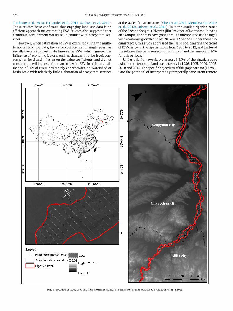

8 ndicat

TTeev

tuiscmb

74 B. Fu et al. / Ecological I

ianhong et al., 2010; Fernandes et al., 2011; Scolozzi et al., 2012).hese studies have confirmed that engaging land use data is anfficient approach for estimating ESV. Studies also suggested thatconomic development would be in conflict with ecosystem ser-ices.

However, when estimation of ESV is exercised using the multi-emporal land use data, the value coefficients for single year hassually been used to estimate time-series ESVs, which ignored the

nfluence of economic factors, such as changes in price level, con-

umption level and inflation on the value coefficients, and did notonsider the willingness of human to pay for ESV. In addition, esti-ation of ESV of rivers has mainly concentrated on watershed or

asin scale with relatively little elaboration of ecosystem services

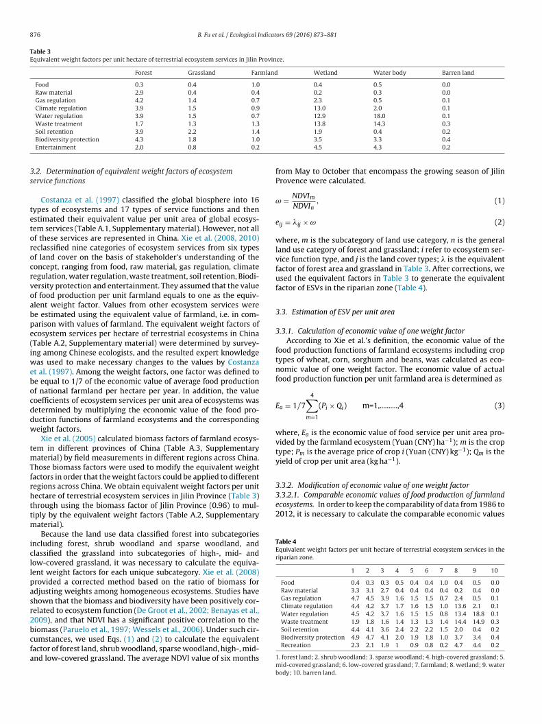
Fig. 1. Location of study area and field measured points. The

ors 69 (2016) 873–881

at the scale of riparian zones (Chen et al., 2012; Mendoza-Gonzálezet al., 2012; Luisetti et al., 2014). Take the studied riparian zonesof the Second Songhua River in Jilin Province of Northeast China asan example, the areas have gone through intense land use changeswith economic growth during 1986–2012 periods. Under these cir-cumstances, this study addressed the issue of estimating the trendof ESV change in the riparian zone from 1986 to 2012, and exploredthe relationship between economic growth and the amount of ESVfor this periods.

Under this framework, we assessed ESVs of the riparian zoneusing multi-temporal land use datasets in 1986, 1995, 2000, 2005,2010 and 2012. The specific objectives of this paper are to: (1) eval-uate the potential of incorporating temporally concurrent remote

small serial units was based evaluation units (BEUs).

B. Fu et al. / Ecological Indicators 69 (2016) 873–881 875

Table 11:100000 Land-use categories in the riparian zone.

Categories Subcategories

Forest area forest land, sparse woodland, shrub woodlandGrassland high-covered grassland,mid-covered grassland,low-covered grasslandFarmland paddy field, glebe fieldWetland riverine wetlands

alkalinspor

s(fstt

2

2

zcsatT

1mosoi2

2

2

bAiiflmip

bRmi

2

epTSptT

source for the main channels. Then, the polygon of the riparian zonewas separated using lines perpendicular to the river centerlines.This process generated 520 BEUs (Fig. 1).

Table 2Multi-temporal Landsat images.

Year Acquisition Date Sensors

Path/Row 118/29 Path/Row 119/29

1986 18 May 1987 6 May 1986 MSS2 Jun 1986 1 Jun 198620 Sep 1986 19 Sep 1986

1995 11Jun 1996 2 Jun 1996 MSS18 Jul 1995 11 Jul 1995 TM29 Sep 1995 20 Sep 1995

2001 25 Jun 2001 11 Aug 200112 Aug 20017 Oct 2001

24 Jun 2001 ETM+28 Sep 2001

2005 10 Oct 2005 29 May 2006 TM17 Aug 200617 Oct 2005

Water body rivers, reservoirs fishery and lakesBarren land lands unused or difficult for using, saline-Build up industrial and commercial, residential, tra

ensing data to adjust the equivalent weight factors for each phase;2) explore the impact of the relationship between willing to payor ecosystem services and socio-economic development on a time-eries ESV; (3) understand the trend of the riparian ESV from 1986o 2012 to identify economic and environmental factors impactinghe ESV of the riparian zone.

. Study area and data source

.1. Study area

This study was conducted in a 360 km section of the riparianone of the Second Songhua River from Fengman reservoir to San-ha estuary. The Second Songhua River is the largest tributary andource of water of Songhua River, which flows through major citiesnd counties of the Jilin Province in Northeast China (Fig. 1). Theopography variation of the river basin is between 54 to 2667 m.he river basin receives about 700 mm of annual rainfall.

Significant land use changes had occurred in the region between986 and 2012. The ecosystem of the riparian zone experienceduch damages by conversion of forested areas to arable land,

vergrazing, construction of transportation infrastructure, urbanprawl, sand mining, tourism development, reclaimed wetland andther human activities. An investigation and evaluation of ecolog-cal stability and integrality of the riparian zone was initiated in012 by the Chinese Ministry of Water Resources.

.2. Data source

.2.1. Land-cover data and other dataThis study adopted the land-use maps (1:100,000) developed

y the Resources and Environment Science Data Center, Chinesecademy of sciences. These land-use datasets were developed

n 1986, 1995, 2000, 2005, 2010 and 2012, respectively, whichncluded information of land-use categories in forest area, grassland,armland, wetland, water body, barren land and build up (Table 1). Theand-use dataset of 2012 was generated by updating the land-use

ap of 2010 with Landsat 8 Operational Land Imager (OLI) imagesn 2013 according to the interpretation keys from field measuredoints identified in Fig. 1.

Other datasets included 1:500,000 geomorphic map compiledy the Institute of Geographic Sciences and Natural Resourcesesearch, Chinese Academy of Sciences; 1:100,000 topographicap and Shuttle Radar Topography Mission (SRTM) generated Dig-

tal Elevation Model data at 90 m spatial resolution.

.2.2. Normalized difference vegetation index dataThis study calculated the average value of Normalized Differ-

nce Vegetation Index (NDVI) of the study area as a corrected scalearameter from May to October in every year using Landsat images.wenty-eight Landsat images from sensors such as Multispectral

canner (MSS), Thematic Mapper (TM), Enhanced Thematic Map-er Plus (ETM + ) and OLI were adopted. These images acquired fromwo paths and rows of 118/29 and 119/29 cover the study area.he selected Landsat images were acquired from May to October

ne landtation ends

in 1986, 1995, 2000, 2005, 2013 and 2014 (Table 2). The spatialresolution of Landsat TM, ETM+ and OLI is 30m × 30m. The spatialresolution of Landsat MSS is 78m × 78m.

2.2.3. Socio-economic dataSocio-economic data were adopted from China Statistical Year-

book for 1986–2013 and China Agricultural Product Cost BenefitCompilation for 1986–2013 by National Bureau of Statistics ofChina, including the average price of main crop types of wheat,corn, sorghum and beans, yield of crop per unit area and the valueof Engel coefficient.

3. Methods

3.1. Basic evaluation units and riparian zone

In this study, the riparian zone is defined as a narrow strip of landfrom the first terrace down to the water’s edge, according to the flu-vial geomorphology (Zaimes, 2007). We extracted the riparian zonefrom 1:500,000 geomorphic map and 1:100,000 topographic mapwhich consists of areas with the width, from 296 m to 4700 m andelevation from 120 m to 350 m (Fig. 1). The study area was parti-tioned into four sections and each section was divided into discreteunits, named basic evaluation units (BEUs). The BEUs were definedas homogeneous river reaches not longer than 600 m following theChinese Ministry of Water Resources technical document (Ministryof Water Resources of the People’s Republic of China, 2010), andthe length was used as a splitting criterion. Hence, the river reachretrieved as a single feature GIS polygon was split from mouth to

30 May 2006 ETM+18 Aug 2006

2012 25 May 2013 1 Jun 2013 OLI16 Oct 2014 7 Oct 2014

876 B. Fu et al. / Ecological Indicators 69 (2016) 873–881

Table 3Equivalent weight factors per unit hectare of terrestrial ecosystem services in Jilin Province.

Forest Grassland Farmland Wetland Water body Barren land

Food 0.3 0.4 1.0 0.4 0.5 0.0Raw material 2.9 0.4 0.4 0.2 0.3 0.0Gas regulation 4.2 1.4 0.7 2.3 0.5 0.1Climate regulation 3.9 1.5 0.9 13.0 2.0 0.1Water regulation 3.9 1.5 0.7 12.9 18.0 0.1Waste treatment 1.7 1.3 1.3 13.8 14.3 0.3

3s

tetorocrvoabpe(iwebocddw

tmTfrhttm

icllpasr2bcfa

3.3.2.1. Comparable economic values of food production of farmlandecosystems. In order to keep the comparability of data from 1986 to2012, it is necessary to calculate the comparable economic values

Table 4Equivalent weight factors per unit hectare of terrestrial ecosystem services in theriparian zone.

1 2 3 4 5 6 7 8 9 10

Food 0.4 0.3 0.3 0.5 0.4 0.4 1.0 0.4 0.5 0.0Raw material 3.3 3.1 2.7 0.4 0.4 0.4 0.4 0.2 0.4 0.0Gas regulation 4.7 4.5 3.9 1.6 1.5 1.5 0.7 2.4 0.5 0.1Climate regulation 4.4 4.2 3.7 1.7 1.6 1.5 1.0 13.6 2.1 0.1Water regulation 4.5 4.2 3.7 1.6 1.5 1.5 0.8 13.4 18.8 0.1Waste treatment 1.9 1.8 1.6 1.4 1.3 1.3 1.4 14.4 14.9 0.3Soil retention 4.4 4.1 3.6 2.4 2.2 2.2 1.5 2.0 0.4 0.2Biodiversity protection 4.9 4.7 4.1 2.0 1.9 1.8 1.0 3.7 3.4 0.4

Soil retention 3.9 2.2 1.4Biodiversity protection 4.3 1.8 1.0Entertainment 2.0 0.8 0.2

.2. Determination of equivalent weight factors of ecosystemervice functions

Costanza et al. (1997) classified the global biosphere into 16ypes of ecosystems and 17 types of service functions and thenstimated their equivalent value per unit area of global ecosys-em services (Table A.1, Supplementary material). However, not allf these services are represented in China. Xie et al. (2008, 2010)eclassified nine categories of ecosystem services from six typesf land cover on the basis of stakeholder’s understanding of theoncept, ranging from food, raw material, gas regulation, climateegulation, water regulation, waste treatment, soil retention, Biodi-ersity protection and entertainment. They assumed that the valuef food production per unit farmland equals to one as the equiv-lent weight factor. Values from other ecosystem services weree estimated using the equivalent value of farmland, i.e. in com-arison with values of farmland. The equivalent weight factors ofcosystem services per hectare of terrestrial ecosystems in ChinaTable A.2, Supplementary material) were determined by survey-ng among Chinese ecologists, and the resulted expert knowledge

as used to make necessary changes to the values by Costanzat al. (1997). Among the weight factors, one factor was defined toe equal to 1/7 of the economic value of average food productionf national farmland per hectare per year. In addition, the valueoefficients of ecosystem services per unit area of ecosystems wasetermined by multiplying the economic value of the food pro-uction functions of farmland ecosystems and the correspondingeight factors.

Xie et al. (2005) calculated biomass factors of farmland ecosys-em in different provinces of China (Table A.3, Supplementary

aterial) by field measurements in different regions across China.hose biomass factors were used to modify the equivalent weightactors in order that the weight factors could be applied to differentegions across China. We obtain equivalent weight factors per unitectare of terrestrial ecosystem services in Jilin Province (Table 3)hrough using the biomass factor of Jilin Province (0.96) to mul-iply by the equivalent weight factors (Table A.2, Supplementary

aterial).Because the land use data classified forest into subcategories

ncluding forest, shrub woodland and sparse woodland, andlassified the grassland into subcategories of high-, mid- andow-covered grassland, it was necessary to calculate the equiva-ent weight factors for each unique subcategory. Xie et al. (2008)rovided a corrected method based on the ratio of biomass fordjusting weights among homogeneous ecosystems. Studies havehown that the biomass and biodiversity have been positively cor-elated to ecosystem function (De Groot et al., 2002; Benayas et al.,009), and that NDVI has a significant positive correlation to theiomass (Paruelo et al., 1997; Wessels et al., 2006). Under such cir-

umstances, we used Eqs. (1) and (2) to calculate the equivalentactor of forest land, shrub woodland, sparse woodland, high-, mid-nd low-covered grassland. The average NDVI value of six months

1.9 0.4 0.23.5 3.3 0.44.5 4.3 0.2

from May to October that encompass the growing season of JilinProvence were calculated.

ω = NDVIm

NDVIn, (1)

eij = �ij × ω (2)

where, m is the subcategory of land use category, n is the generalland use category of forest and grassland; i refer to ecosystem ser-vice function type, and j is the land cover types; � is the equivalentfactor of forest area and grassland in Table 3. After corrections, weused the equivalent factors in Table 3 to generate the equivalentfactor of ESVs in the riparian zone (Table 4).

3.3. Estimation of ESV per unit area

3.3.1. Calculation of economic value of one weight factorAccording to Xie et al.’s definition, the economic value of the

food production functions of farmland ecosystems including croptypes of wheat, corn, sorghum and beans, was calculated as eco-nomic value of one weight factor. The economic value of actualfood production function per unit farmland area is determined as

Ea = 1/74∑

m=1

(Pi × Qi) m=1,..........,4 (3)

where, Ea is the economic value of food service per unit area pro-vided by the farmland ecosystem (Yuan (CNY) ha−1); m is the croptype; Pm is the average price of crop i (Yuan (CNY) kg−1); Qm is theyield of crop per unit area (kg ha−1).

3.3.2. Modification of economic value of one weight factor

Recreation 2.3 2.1 1.9 1 0.9 0.8 0.2 4.7 4.4 0.2

1. forest land; 2. shrub woodland; 3. sparse woodland; 4. high-covered grassland; 5.mid-covered grassland; 6. low-covered grassland; 7. farmland; 8. wetland; 9. waterbody; 10. barren land.

B. Fu et al. / Ecological Indicators 69 (2016) 873–881 877

Table 5The calibrated parameters of economic value per unit area of ecosystem services.

Years � Comparable value($a ha−1) Dynamic correction

1986 0.8 154.8 0.21995 0.6 297.9 0.22000 0.7 189.6 0.42005 0.6 255.6 0.4

tf

E

itftG

3waenpwaltd(posw

E

wdcf

3tSetTebvaJ

3

ocPl

u

Table 6The of economic value per unit area of ecosystem services ($ · ha−1).

1986 1995 2000 2005 2012

1 885.7 1324.9 1347.5 1789.2 2808.92 836.9 1251.9 1273.4 1690.7 2654.33 731.3 1093.9 1112.6 1477.3 2319.34 360.8 539.7 549.0 728.9 1144.35 337.2 504.4 513.1 681.2 1069.56 327.1 489.3 497.7 660.8 1037.47 237.8 355.7 361.8 480.4 754.18 1648.6 2466.0 2508.2 3330.3 5228.49 1365.0 2041.9 2076.8 2757.5 4329.110 41.8 62.6 63.7 84.5 132.7

2012 0.5 382.5 0.5

a 1$ (USD) = 6.21Yuan (CNY) in 2014.

o eliminate influence of price level, inflation and other economicactors.

an = Eam/�n

�m× GDPm

GDPn× 100 (4)

n this equation, m represents the current year and n representshe past year. Eam is the current economic value of food service ofarmland ecosystem in riparian zone for year m, Ean is calculated byhe Eam value in year n during the study period. GDP is the Chineseross Domestic Product and is the yearly GDP index.

.3.2.2. Temporal correction based on pearl growth curve model. Theillingness to pay is one of the basic concepts and theory for evalu-

ting value of non-market goods and ecological services (De Groott al., 2002). The realization of ESV needs to combine the willing-ess of local people to pay. The awareness of people willingness toay for ecosystem services is described as in the “S” shaped patternith social-economic development. The awareness is low while

t the lower stage of economic development and the awarenessevel enhances relatively slow. When people reach a well-off stage,he requirement for environmental comfort service may increaseramatically until it becomes saturated. The pearl growth curvePGC) model has been very frequently used to describe the S-shaperocesses between limited resources and socio-economic devel-pment (Xu et al., 2013; Yue et al., 2011; Kwasnicki, 2013). In thistudy, we used the PGC model to correct the economic value of oneeight factor from 1986 to 2012.

= 11 + e−t

× Ea t = 1En

− 3 (5)

here, E is the ESV per unit in year m, t is the socio-economicevelopment indicator, e is the natural logarithm, En is the Engeloefficient between 0 and 1. Ea is the food production value ofarmland ecosystems in the current year.

.3.2.3. Spatial scale correction. Ecosystem services are suppliedo the economic value at a range of spatial and temporal scales.takeholders at different spatial scales attach different values tocosystem services (Hein et al., 2006). Compared to the territory ofhe Jilin Province, the riparian zone is considered in a smaller scale.he economic value of one weight factor for riparian zone is differ-nt from Jilin Province. Therefore, we still used the ratio of biomassetween Jilin Province and riparian zone to calibrate the economicalue of one weight factor, specific calculation of ratio between theverage of NDVI in the riparian zone and the average of NDVI inilin Province (Eq. (6)).

.3.3. Calculation of ESV per unit area in riparian zoneAfter temporal and spatial scale correction, the economic value

f ecosystem services per unit area in the riparian zone was cal-ulated by multiplying the equivalent weight factors of ESV in Jilinrovince (Table 4) by economic value of food production of farm-

and ecosystem services in the study area (Eq. (7)).

= NDVI1

NDVI0(6)

1. forest land; 2. shrub woodland; 3. sparse woodland; 4. high-covered grassland; 5.mid-covered grassland; 6. low-covered grassland; 7. farmland; 8. wetland; 9. waterbody; 10. barren land.

Eij = eij × u × E (i = 1, 2, · · · · ··, 9; j=1,2, · · · · · ·,10) (7)

NDVI0 is the average value of NDVI in Jilin Province; NDVI1 is theaverage value of NDVI in the riparian zone calculated by Landsatimages; i is to ecosystem service function type, and j is the land usecategory; E is the economic value of food production of farmlandecosystem after temporal correction; eij is the equivalent factor ofthe ecosystem service function i of a land cover type j in Table 4. Eij

is the value per unit area of ecosystem service function i of a landcover type j.

3.4. Calculation of ESV

ESV =9∑

i=1

10∑

j=1

Sj × Eij (8)

where, Sj is the area of ecosystem type j, Eij is the value per unitarea of ecosystem services i of land cover type j.

3.5. Ecosystem sensitivity analysis

The biomes used as proxies for land cover types are clearly notperfect matches, coupled with error introduced when correctingthe coefficients of ESV with NDVI and a PGC model. Sensitivity anal-yses were essential to be conducted to test the percentage changein the ESV for a given percentage change in a value coefficient. Ineach analysis, the coefficient of sensitivity (CS) was calculated bythe standard economic concept of elasticity (Kreuter et al., 2001).

CS = (ESVj − ESVi)/ESVi

(VCjk − VCik)/VCik(9)

where ESV is the estimated ecosystem services value, VC is the valuecoefficients, i and j are the initial and adjusted values, respectively.K is land cover types. If CS is greater than unity, the estimated ESV iselastic with respect to that value coefficient. While if CS is less thanone, the estimated ESV is considered to be inelastic. The greater theproportional change in the ESV relative to the proportional changein the value coefficient, the more critical is the use of an accurateecosystem value coefficient (Kreuter et al., 2001).

4. Results

4.1. Economic value per unit area of ecosystem services

The value per unit area of ecosystem service was obtained aftera series of corrections using the parameters listed in Table 5. The

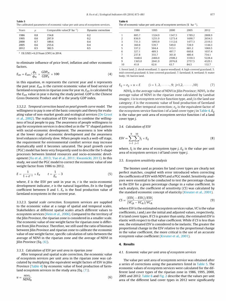
economic values of ecosystem services were calculated for the dif-ferent land cover types of the riparian zone in 1986, 1995, 2000,2005 and 2012. Table 6 and Fig. 2 describe that the values per unitarea of the different land cover types in 2012 were significantly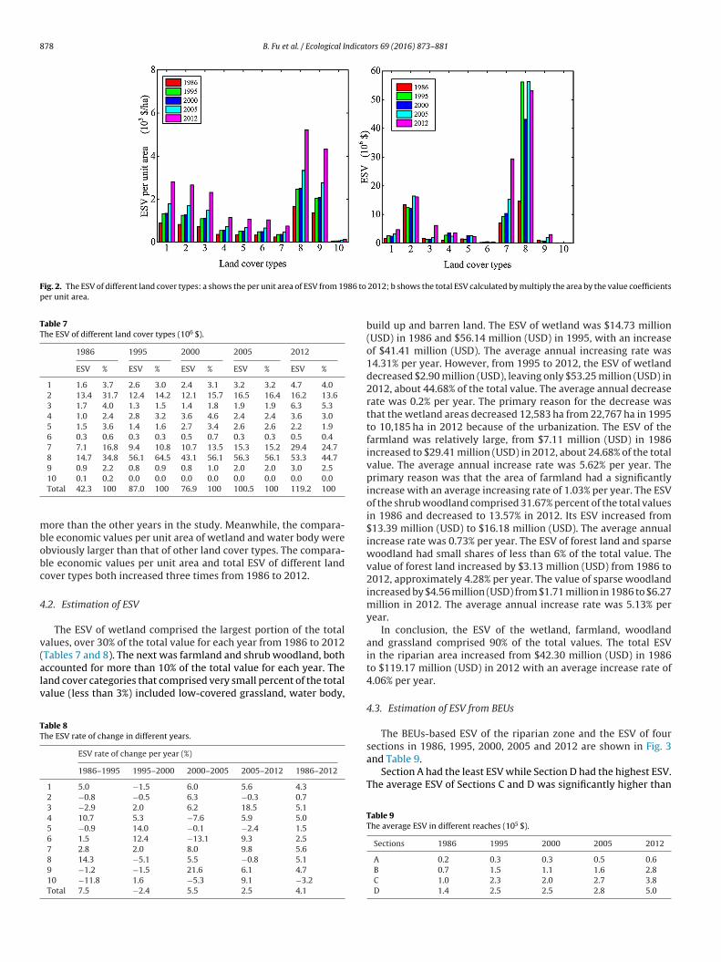

878 B. Fu et al. / Ecological Indicators 69 (2016) 873–881

Fig. 2. The ESV of different land cover types: a shows the per unit area of ESV from 1986 toper unit area.

Table 7The ESV of different land cover types (106 $).

1986 1995 2000 2005 2012

ESV % ESV % ESV % ESV % ESV %

1 1.6 3.7 2.6 3.0 2.4 3.1 3.2 3.2 4.7 4.02 13.4 31.7 12.4 14.2 12.1 15.7 16.5 16.4 16.2 13.63 1.7 4.0 1.3 1.5 1.4 1.8 1.9 1.9 6.3 5.34 1.0 2.4 2.8 3.2 3.6 4.6 2.4 2.4 3.6 3.05 1.5 3.6 1.4 1.6 2.7 3.4 2.6 2.6 2.2 1.96 0.3 0.6 0.3 0.3 0.5 0.7 0.3 0.3 0.5 0.47 7.1 16.8 9.4 10.8 10.7 13.5 15.3 15.2 29.4 24.78 14.7 34.8 56.1 64.5 43.1 56.1 56.3 56.1 53.3 44.79 0.9 2.2 0.8 0.9 0.8 1.0 2.0 2.0 3.0 2.5

mbobc

4

v(alv

TT

10 0.1 0.2 0.0 0.0 0.0 0.0 0.0 0.0 0.0 0.0Total 42.3 100 87.0 100 76.9 100 100.5 100 119.2 100

ore than the other years in the study. Meanwhile, the compara-le economic values per unit area of wetland and water body werebviously larger than that of other land cover types. The compara-le economic values per unit area and total ESV of different landover types both increased three times from 1986 to 2012.

.2. Estimation of ESV

The ESV of wetland comprised the largest portion of the totalalues, over 30% of the total value for each year from 1986 to 2012Tables 7 and 8). The next was farmland and shrub woodland, both

ccounted for more than 10% of the total value for each year. Theand cover categories that comprised very small percent of the totalalue (less than 3%) included low-covered grassland, water body,

able 8he ESV rate of change in different years.

ESV rate of change per year (%)

1986–1995 1995–2000 2000–2005 2005–2012 1986–2012

1 5.0 −1.5 6.0 5.6 4.32 −0.8 −0.5 6.3 −0.3 0.73 −2.9 2.0 6.2 18.5 5.14 10.7 5.3 −7.6 5.9 5.05 −0.9 14.0 −0.1 −2.4 1.56 1.5 12.4 −13.1 9.3 2.57 2.8 2.0 8.0 9.8 5.68 14.3 −5.1 5.5 −0.8 5.19 −1.2 −1.5 21.6 6.1 4.710 −11.8 1.6 −5.3 9.1 −3.2Total 7.5 −2.4 5.5 2.5 4.1

2012; b shows the total ESV calculated by multiply the area by the value coefficients

build up and barren land. The ESV of wetland was $14.73 million(USD) in 1986 and $56.14 million (USD) in 1995, with an increaseof $41.41 million (USD). The average annual increasing rate was14.31% per year. However, from 1995 to 2012, the ESV of wetlanddecreased $2.90 million (USD), leaving only $53.25 million (USD) in2012, about 44.68% of the total value. The average annual decreaserate was 0.2% per year. The primary reason for the decrease wasthat the wetland areas decreased 12,583 ha from 22,767 ha in 1995to 10,185 ha in 2012 because of the urbanization. The ESV of thefarmland was relatively large, from $7.11 million (USD) in 1986increased to $29.41 million (USD) in 2012, about 24.68% of the totalvalue. The average annual increase rate was 5.62% per year. Theprimary reason was that the area of farmland had a significantlyincrease with an average increasing rate of 1.03% per year. The ESVof the shrub woodland comprised 31.67% percent of the total valuesin 1986 and decreased to 13.57% in 2012. Its ESV increased from$13.39 million (USD) to $16.18 million (USD). The average annualincrease rate was 0.73% per year. The ESV of forest land and sparsewoodland had small shares of less than 6% of the total value. Thevalue of forest land increased by $3.13 million (USD) from 1986 to2012, approximately 4.28% per year. The value of sparse woodlandincreased by $4.56 million (USD) from $1.71 million in 1986 to $6.27million in 2012. The average annual increase rate was 5.13% peryear.

In conclusion, the ESV of the wetland, farmland, woodlandand grassland comprised 90% of the total values. The total ESVin the riparian area increased from $42.30 million (USD) in 1986to $119.17 million (USD) in 2012 with an average increase rate of4.06% per year.

4.3. Estimation of ESV from BEUs

The BEUs-based ESV of the riparian zone and the ESV of four

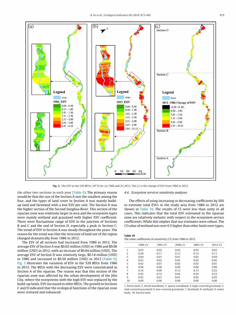
sections in 1986, 1995, 2000, 2005 and 2012 are shown in Fig. 3and Table 9.

Section A had the least ESV while Section D had the highest ESV.The average ESV of Sections C and D was significantly higher than

Table 9The average ESV in different reaches (105 $).

Sections 1986 1995 2000 2005 2012

A 0.2 0.3 0.3 0.5 0.6B 0.7 1.5 1.1 1.6 2.8C 1.0 2.3 2.0 2.7 3.8D 1.4 2.5 2.5 2.8 5.0

B. Fu et al. / Ecological Indicators 69 (2016) 873–881 879

d (b)

twfutrwTBTrc

amaiFtSrCbCw

cases. This indicates that the total ESV estimated in the riparianzone are relatively inelastic with respect to the ecosystem servicecoefficients. While this implies that our estimates were robust. TheCS value of wetland was over 0.5 higher than other land cover types,

Table 10The value coefficients of sensitivity (CS) from 1986 to 2012.

1986 CS 1995 CS 2000 CS 2005 CS 2012 CS

1 0.03 0.02 0.03 0.03 0.032 0.28 0.11 0.13 0.12 0.113 0.04 0.01 0.01 0.02 0.044 0.02 0.02 0.05 0.02 0.025 0.02 0.01 0.02 0.02 0.016 0.00 0.00 0.00 0.00 0.007 0.16 0.09 0.12 0.13 0.228 0.43 0.72 0.64 0.65 0.539 0.02 0.01 0.01 0.02 0.03

Fig. 3. The ESV in the 520 BEUs (105 $) for (a) 1986 an

he other two sections in each year (Table 9). The primary reasonould be that the size of the Section A was the smallest among the

our, and the types of land cover in Section A was mainly build-p land and farmland with a low ESV per unit. The Section D washe higher section of the Second Songhua River. This section of theiparian zone was relatively larger in area and the ecosystem typesere mainly wetland and grassland with higher ESV coefficient.

here were fluctuations range of ESV in the junction of Sections and C and the end of Section D, especially a peak in Section C.he trend of ESV in Section A was steady throughout the years. Theeason for the trend was that the structure of land use of the regionhanged dramatically from 1986 to 2012.

The ESV of all sections had increased from 1986 to 2012. Theverage ESV of Section A was $0.02 million (USD) in 1986 and $0.06illion (USD) in 2012, with an increase of $0.04 million (USD). The

verage ESV of Section D was relatively large, $0.14 million (USD)n 1986 and increased to $0.50 million (USD) in 2012 (Table 9).ig. 3 illustrates the variation of ESV in the 520 BEUs from 1986o 2012. The BEUs with the decreasing ESV were concentrated inection A of the riparian. The reason was that this section of theiparian zone was affected by the urban development of the Jilin

ity, where the ecosystems with the high ESV was replaced by theuild-up lands. ESV increased in other BEUs. The growth in Sections

and D indicated that the ecological functions of the riparian zoneere restored and enhanced.

2012. The (c) is the change of ESV from 1986 to 2012.

4.4. Ecosystem services sensitivity analyses

The effects of using increasing or decreasing coefficients by 50%to estimate total ESVs in the study area from 1986 to 2012 areshown in Table 10. The results of CS were less than unity in all

10 0.00 0.00 0.00 0.00 0.00

1. forest land; 2. shrub woodland; 3. sparse woodland; 4. high-covered grassland; 5.mid-covered grassland; 6. low-covered grassland; 7. farmland; 8. wetland; 9. waterbody; 10. barren land.

880 B. Fu et al. / Ecological Indicat

Table 11The area of different land cover types in the riparian zone.

1986 1995 2000 2005 2012

area(ha) % area(ha) % area(ha) % area(ha) % area(ha) %

1 1788 2.6 1952 2.7 1785 2.5 1794 2.6 1677 2.52 16004 22.8 9889 13.8 9506 13.2 9737 13.9 6094 9.23 2333 3.3 1168 1.6 1269 1.8 1292 1.8 2701 4.14 2773 4.0 5112 7.2 6493 9.0 3294 4.7 3126 4.75 4457 6.4 2728 3.8 5161 7.2 3867 5.5 2086 3.16 763 1.1 594.0 0.8 1047 1.5 390 0.6 461 0.77 29886 42.7 26344 36.9 28625 39.8 31744 45.3 39003 58.88 8938 12.8 22767 31.9 17191 23.9 16915 24.2 10185 15.39 674 1.0 397 0.6 362 0.5 726 1.0 699 1.1

fwoCtoe

4

datc

4

fii1idTa13tiag

TL

1mb

10 2445 3.5 465 0.7 495 0.7 283 0.4 331 0.511 3874 5.2 3607 4.8 3872 5.1 4058 5.5 4954 6.9

ollowed farmland and shrub woodland. The CS value of shruboodland decreased 0.17 from 1986 to 2012. While the CS value

f farmland and wetland increased 0.06 and 0.1, respectively. TheS value of other land cover types was in the near-zero stable condi-ion. These results indicates that the use of an accurate coefficientsf wetland, farmland, and shrub woodland are very important tostimate the total ESV.

.5. Driving factors of ESV change

The ESV of riparian zone increased from 1986 to 1995, thenecrease from 1995 to 2005, lastly increase from 2005 to 2012gain. The primary reasons and affecting factors for this fluctua-ion were changes of land use and the difference of economic valueoefficients per unit area.

.5.1. Change of land useFrom Tables 11 and 12, the area of build-up area had an increase

rom 3874 ha in 1986 to 4,594 ha in 2012. This implied the increasen the population and urbanization. Under the impact of human-nduced land use changes the area of farmland was 29,886 ha in986 and 39,003 ha in 2012, increase by 9118 ha, at an average

ncreasing rate of 1.03% per year. Meanwhile, the wetland areaecreased by 12,583 ha from 22,767 ha in 1995 to 10,185 ha in 2012.he average annual decrease rate was 3.05% per year. Besides, therea of shrub woodland decreased by 9900 ha from 16,004 ha in995 to 6,094 ha in 2012, the average annual decrease rate was.65% per year. The area of forest land decreased by 11 ha from 1986

o 2012, approximately 0.25% per year. The area of sparse woodlandncreased by 368 ha from 2333 ha in 1986 to 2,701 ha in 2012, theverage annual increase rate was 0.57% per year. The three types ofrassland also had small size in area, less than 10% of the total area.

able 12and use rate of change in the riparian zone.

Land use rate of change per year (%)

1986–1995 1995–2000 2000–2005 2005–2012 1986–2012

1 0.9 −1.8 0.1 −1.0 −0.32 −4.7 −0.8 0.5 −6.5 −3.73 −6.7 1.7 0.4 11.1 0.64 6.3 4.9 −12.7 −0.8 0.55 −4.8 13.6 −5.6 −8.4 −2.96 −2.5 12.0 −17.9 2.4 −1.97 −1.3 1.7 2.1 3.0 1.08 9.8 −5.5 −0.3 −7.0 0.59 −5.1 −1.8 14.9 −0.5 0.110 0.9 −1.8 0.1 −1.0 −0.311 −0.7 1.4 0.9 2.9 1.0

. forest land; 2. shrub woodland; 3. sparse woodland; 4. high-covered grassland; 5.id-covered grassland; 6. low-covered grassland; 7. farmland; 8. wetland; 9. water

ody; 10. barren land; 11. build up.

ors 69 (2016) 873–881

The high-covered grassland increased in area from 2773 ha in 1986to 3,126 ha in 2012, with an average growth rate of 0.57% per year.The area of other grassland was with an average decrease rate of2% ∼ 3% per year. In conclusion, human-land use change controlledthe trend of ESV of the riparian from 1986 to 2012.

4.5.2. The difference of economic value coefficients per unit areaThe economic value coefficients per unit area were deter-

mined by comparable economic values of food production, people’swillingness to pay. Socio-economic data from China StatisticalYearbook showed that the average price of crop had trebled andthe yield of crop per unit area had greatly increased from 1986to 2012. The price of rice rose from 0.51 Yuan (CNY)/kg to 2.99Yuan (CNY)/kg, and the yield of rice increased from 4959 kg/ha to7587 kg/ha. The increase of the price and yield of crop also causedthe comparable economic values of food production. According tothe PGC model, the people’s willingness to pay for ecological ser-vice would gradually enhance with the economic development.The GDP of Jilin Province had a great growth from 31.56 billionYuan (CNY) to 343.31 billion Yuan (CNY). Besides, citizens and gov-ernment pay more attention to the ecological environment of theriparian zone. This attention also would cause the change of landuse, and increase those land use categories with high ESV.

5. Conclusions and discussion

The method used to estimate ESV in this study derived the ESVof riparian zone from multiplying the corrected value of coefficientsper unit and the area of corresponding land cover types. Giventhat ecosystem services are supplied at various spatial and tem-poral scales (Hein et al., 2006), we used NDVI and a PGC model tomodify equivalent weight factors and value coefficients of differ-ent land cover types. The accuracy of the corrected weight factors isalways challenging because of ecosystem complexity. For instance,the weight factor for shrub woodland is derived from multiplyingthe ratio of NDVI and corresponding weight factor of the generalland use category of forest. It is an approximate estimation usingpositive correlation between NDVI and biomass, and need furthervalidation. However, the results of our sensitivity analysis suggestthat despite uncertainties in the value coefficients, the approachcan produce useful and robust results. By calculating ESV from 1986to 2012 and analyzing changes, uncertainties and errors could thusbe offset. In addition, it is important to realize that accurate coef-ficients are often less critical for time series than cross-sectionalanalysis because coefficients tend to affect estimates of directionalchange less than estimates of the magnitude of ecosystem valuesat specific points in time. This study is primarily concerned withchanges in ESV over time.

The ESV of the entire studied riparian zone increased $76.9 mil-lion (USD) from $42.30 million (USD) in 1986 to $119.17 million(USD) in 2012 with the economic growth. An average ESV of individ-ual BEUs increased from $0.08 million (USD) in 1986 to $0.3 million(USD) in 2012. This value indicates that the riparian zone is a sig-nificant economic resource and has fragile environments, whichis affected by both environmental and human-induced stresses.Obscured by the increase of the total ESV, the proportion of the con-tributed by wetland decreased 19.8% from 64.5% in 1995 to 44.7% in2012. The ESV of farmland accounted for the increase in ESV of 10%from 16.8% in 1986 to 24.7% in 2012, especially during 2005–2012periods. The ESV of shrub woodland accounted for the total ESV

decreased from 31.7% in 1986 to 13.57% in 2012. Reductions ofwetland and shrub woodland combined with increases in farm-land suggested that without a land use plan for the riparian zonethat protects wetlands, high-covered grassland, and woodland, a

ndicat

bt

msftsoistfedenre

rlAicmaetsar

A

dafaw

A

i0

R

B

B

B

C

B. Fu et al. / Ecological I

alance between economic development and the natural ecosys-em would not be reached.

This study utilized the economic development level factor toodify the value coefficients and to estimate the value of ecosystem

ervices. The introduction of this factor not only provided an insightor exploring the interaction mechanism between natural ecosys-ems and economic systems, but also fills in the gaps between thetatic value coefficients and estimation time-series ESVs. The valuef PGC model increased from 0.2 in 1986 to 0.5 in 2012. This resultndicates that the awareness and willingness to pay for ecosystemervices is gradually raised from 1986 to 2012 with the growth ofhe local economy. While ESV as a proportion of GDP decreasedrom 8% in 1986 to 2% in 2012. These results indicates that thecosystem service level is relatively low compared to the economicevelopment level, and the awareness and willingness to pay forcosystem services increase has been lower than the level of eco-omic development. Sustainable development is essential for theiparian zone. A compromise between economic development andcological protection must therefore be addressed.

This study provided a case of ecosystem service valuation iniparian zone. BEUs-based ESV indicates that Section D with wet-and and forest land area possesses the highest ESV while Section

with dominated urban area has the lowest ESV. The ESV of BEUsn the Section A has negative growth from 1986 to 2012. Theseonclusions are very useful for selecting representative measure-ent sections and sites from riparian zones for field evaluation. In

ddition, BEUs-based method is able to continuously monitor andvaluate riparian ecological conditions and services over time whileraditional monitoring methods usually use the results from mea-uring sites for field evaluation. The BEUs-based method allows for

more comprehensive evaluation of the riparian zone ESV. Futureesearch should include validation with field measurements.

cknowledgments

This study was funded by the National Natural Science Foun-ation of China (Grant No. 41271113). The principal authorppreciates the scholarship from the Chinese Academy of Sciencesor sponsoring his research in the University of Rhode Island. Weppreciate anonymous reviewers for their constructive commentshich help improve the quality of this manuscript.

ppendix A. Supplementary data

Supplementary data associated with this article can be found,n the online version, at http://dx.doi.org/10.1016/j.ecolind.2016.5.048.

eferences

arquın, J., Fernández, D., Alvarez-Cabria, M., Penas, F., 2011. Riparian quality andhabitat heterogeneity assessment in Cantabrian Rivers. Limnetica 30 (2),329–346.

enayas, J.M.R., Newton, A.C., Diaz, A., Bullock, J.M., 2009. Enhancement ofbiodiversity and ecosystem services by ecological restoration: a meta-analysis.Science 325 (5944), 1121–1124.

oyd, J., Banzhaf, S., 2007. What are ecosystem services? The need for standardizedenvironmental accounting units. Ecol. Econ. 63 (2), 616–626.

hen, N.W., Li, H.C., Wang, L.H., 2009. A GIS-based approach for mapping direct usevalue of ecosystem services at a county scale: management implications. Ecol.Econ. 68 (11), 2768–2776.

ors 69 (2016) 873–881 881

Chen, Q., Liu, J., Ho, K.C., Yang, Z., 2012. Development of a relative risk model forevaluating ecological risk of water environment in the Haihe River Basinestuary area. Sci. Total Environ. 420, 79–89.

Costanza, R., d’Arge, R., de Groot, R., Farber, S., Grasso, M., Hannon, B., Limburg, K.,Naeem, S., O’Neill, R.V., Paruelo, J., Raskin, R.G., Sutton, P., van den Belt, M.,1997. The value of the world’s ecosystem services and natural capital. Nature387, 253–260.

Daily, G.C. (Ed.), 1997. Nature’s Services: Societal Dependence on NaturalEcosystems. Island Press, Washington, DC, pp. 3–10.

De Groot, R.S., Wilson, M.A., Boumans, R.M.J., 2002. A typo logy for theclassification, description and valuation of ecosystem functions, goods andservices. Ecol. Econ. 41 (3), 393–408.

Fernández, D., Barquín, J., Álvarez-Cabria, M., Penas, F.J., 2014. Land-use coverageas an indicator of riparian quality. Ecol. Indic. 41, 165–174.

Fernandes, M.R., Aguiar, F.C., Ferreira, M.T., 2011. Assessing riparian vegetationstructure and the influence of land use using landscape metrics andgeostatistical tools. Landscape Urban Plann. 99 (2), 166–177.

Hein, L., Van Koppen, K., De Groot, R.S., et al., 2006. Spatial scales, stakeholders andthe valuation of ecosystem services. Ecol. Econ. 57 (2), 209–228.

Ivits, E., Cherlet, M., Mehl, W., Sommer, S., 2009. Estimating the ecological statusand change of riparian zones in Andalusia assessed by multi-temporal AVHHRdatasets. Ecol. Indic. 9 (3), 422–431.

Kreuter, U.P., Harris, H.G., Matlock, M.D., Lacey, R.E., 2001. Change in ecosystemservice values in the San Antonio area, Texas. Ecol. Econ. 39 (3), 333–346.

Kwasnicki, W., 2013. Logistic growth of the global economy and competitivenessof nations. Technol. Forecasting Social Change 80 (1), 50–76.

Li, J., Ren, Z.Y., 2008. Changes in ecosystem service values on the loess plateau inNorthern Shaanxi Province, China. Agricult. Sci. China 7, 606–614.

Luisetti, T., Turner, R.K., Jickells, T., et al., 2014. Coastal Zone Ecosystem Services:from science to values and decision making; a case study. Sci. Total Environ.493, 682–693.

Mendoza-González, G., Martínez, M.L., Lithgow, D., et al., 2012. Land use changeand its effects on the value of ecosystem services along the coast of the Gulf ofMexico. Ecol. Econ. 82, 23–32.

Metzger, M.J., Rounsevell, M.D.A., Acosta-Michlik, L., Leemans, R., Schroter, D.,2006. The vulnerability of ecosystem services to land use change. Agriculture,Ecosyst. Environ. 114, 69–85.

Millennium Ecosystem Assessment, 2003. Ecosystems and Human Well-Being: AFramework for Assessment. Report of the Conceptual Framework WorkingGroup of the Millennium Ecosystem Assessment. Island Press,Washington23–27.

Ministry of Water Resources of the People’s Republic of China, 2010. River (Lake)Health Indicators, Standards and Methods V1.0. The Ministry of WaterResources of the People’s Republic of China, Beijing, China.

Paruelo, J.M., Epstein, H.E., Lauenroth, W.K., Burke, I.C., 1997. ANPP estimates fromNDVI for the central grassland region of the United States. Ecology 78 (3),953–958.

Scolozzi, R., Morri, E., Santolini, R., 2012. Delphi-based change assessment inecosystem service values to support strategic spatial planning in Italianlandscapes. Ecol. Indic. 21, 134–144.

Seppelt, R., Dormann, C.F., Eppink, F.V., Lautenbach, S., Schmidt, S., 2011. Aquantitative review of ecosystem service studies: approaches, shortcomingsand the road ahead. J. Appl. Ecol. 48 (3), 630–636.

Tianhong, L., Wenkai, L., Zhenghan, Q., 2010. Variations in ecosystem service valuein response to land use changes in Shenzhen. Ecol. Econ. 69 (7), 1427–1435.

USDI Bureau of Land Management, 1998. Riparian Area Management: A UserGuide to Assessing Proper Functioning Condition and the Supporting Sciencefor Lotic Areas. Technical Reference TR 1737-15, pp. 4–7.

Wessels, K.J., Prince, S.D., Zambatis, N., MacFadyen, S., Frost, P.E., Van Zyl, D., 2006.Relationship between herbaceous biomass and 1 km2 advanced very highresolution radiometer (AVHRR) NDVI in Kruger National Park, South Africa. Int.J. Remote Sens. 27 (5), 951–973.

Xie, G.D., Xiao, Y., Zhen, L., Lu, C.X., 2005. Study on ecosystem services value of foodproduction in China. Chin. J. Eco-Agricutl. 13 (3), 10–13.

Xie, G.D., Zhen, L., Lu, C.X., Chen, C., 2008. Expert knowledge based valuationmethod of ecosystem services in China. J. Nat. Resour. 23 (5), 911–919.

Xie, G.D., Zhen, L., Lu, C.X., Yu, X., Li, W.H., 2010. Applying value transfer methodfor eco-service valuation in China. J. Resour. Ecol. 1 (1), 51–59.

Xu, L., Yu, B., Yue, W., Xie, X., 2013. A Model for Urban Environment and ResourcePlanning Based on Green GDP Accounting System. Mathematical Problems inEngineering.

Yue, T.X., Jorgensen, S.E., Larocque, G.R., 2011. Progress in global ecologicalmodelling. Ecol. Modell. 222 (14), 2172–2177.

Zaimes, G., 2007. Defining Arizona’s riparian areas and their importance to thelandscape. In: Zaimes, G. (Ed.), Understanding Arizona’s Riparian Areas.University of Arizona Cooperative Extension, Publication #AZ1432, pp. 1–13.