Risk Sharing in Supplier Relations:

An Agency Model for the

Italian Air Conditioning Industry

Arnaldo Camuffo, Andrea Furlan, and Enrico Rettore

MIT-IPC-05-003

June 2005

Risk Sharing in Supplier Relations: An Agency Model for the Italian Air Conditioning Industry Arnaldo Camuffo, Andrea Furlan and Enrico Rettore MIT IPC Working Paper IPC-05-003 June 2005 We apply agency theory to model vertical inter-firm relationships and study risk sharing between manufacturers and first-tier suppliers in the Italian high-precision air conditioning (AC) industry. We explore to what extent buyers and suppliers share risk, and how suppliers’ financial, structural and technological characteristics, used as proxies for environmental uncertainty, moral hazard and risk aversion, are related to the degree of risk-sharing. Improving the modeling techniques used in previous, similar studies, we use regression analysis to test the agency model on the supplier networks (respectively of 50 and 58 suppliers) of two leading Italian high- precision AC manufacturers. The regression analysis shows that both the manufacturers absorb risk to a non-negligible degree, and supports the hypotheses that they absorb more risk a) the bigger are the fluctuations in the supplier’s costs; b) the more risk averse is the supplier; and c) the less severe is the supplier’s moral hazard. We interpret these findings and draw some managerial implications about the design of supply contracts, the optimal allocation of risk across supply chains, and the management of supply networks.

The views expressed herein are the author’s responsibility and do not necessarily reflect

those of the MIT Industrial Performance Center or the Massachusetts Institute of

Technology.

1

Risk Sharing in Supplier Relations:

An Agency Model for the Italian Air Conditioning Industry*

Arnaldo Camuffo Department of Economics

University of Padova Via del Santo 33

35123 Padova, Italy Tel.: +39-049-827-4232 – Fax.: +39-049-827-4211

e-mail: arnaldo.camuffo@unipd.it currently at

Industrial Performance Center – M.I.T. 292 Main Street - E38

Cambridge, MA, 02139-4307 Tel.: (617)-253-0142 – Fax.: (617)-253-7570

e-mail: acamuffo@mit.edu

Andrea Furlan Department of Economics

University of Padova Via del Santo 23

35123 Padova, Italy Tel.: + 39-049-827-3848 – Fax.: +39-049-827-4211

e-mail: andrea.furlan@unipd.it

Enrico Rettore Department of Statistics

Via Cesare Battisti, 241/243 35123 Padova, Italy

Tel.: + 39-049-827-4164 – Fax.: +39-049 827 4170 e-mail: enrico.rettore@unipd.it

June 2005

* We wish to thank Suzanne Berger, Michael Cusumano, Charles Fine, Robert Gibbons, Anna Grandori, Richard Lester, Richard Locke, Michael Piore and Marek Pycia for suggestions and comments on earlier versions. Research funded by MIUR.

2

Risk Sharing in Supplier Relations:

An Agency Model for the Italian Air Conditioning Industry

Abstract

We apply agency theory to model vertical inter-firm relationships and study risk sharing between

manufacturers and first-tier suppliers in the Italian high-precision air conditioning (AC) industry.

We explore to what extent buyers and suppliers share risk, and how suppliers’ financial,

structural and technological characteristics, used as proxies for environmental uncertainty, moral

hazard and risk aversion, are related to the degree of risk-sharing. Improving the modeling

techniques used in previous, similar studies, we use regression analysis to test the agency model

on the supplier networks (respectively of 50 and 58 suppliers) of two leading Italian high-

precision AC manufacturers. The regression analysis shows that both the manufacturers absorb

risk to a nonnegligible degree, and supports the hypotheses that they absorb more risk a) the

bigger are the fluctuations in the supplier’s costs; b) the more risk averse is the supplier; and c)

the less severe is the supplier’s moral hazard. We interpret these findings and draw some

managerial implications about the design of supply contracts, the optimal allocation of risk across

supply chains and the management of supply networks.

Keywords: Risk Sharing; Supplier Relations; Agency Theory; Air Conditioning

3

1. Risk allocation in supplier relations

Risk allocation in supplier relations can be conceptually framed contrasting two opposite

hypotheses: the risk shifting and the risk absorption hypothesis (Kawasaki and McMillan, 1987;

Aoki, 1988; Asanuma and Kikutani, 1992; Yun, 1999; Okamuro, 2001). These hypotheses

underlie different logics in the design of supply contracts and in the management of supplier

relations.

Under the risk-shifting hypothesis, buyers1 seek to minimize purchasing costs transferring to

suppliers the negative effects of business risk. Buyers wish to keep control of suppliers, try to

exploit them to drive costs down and use them as a buffer against business fluctuations. However,

buyers may have limited information about suppliers’ behaviors, technology and costs and

suppliers may take advantage of this private knowledge (so that, in the jargon of theory, there is

potential for moral hazard and hold up problems). In this case, buyers wish to gather as much

detailed information as possible on suppliers (source of business, cost structure, product and

process technologies, manufacturing capacity, inventories and financial position) and monitor, on

the basis of this information, their behaviors and results. Because of their conflict of interests,

buyers and suppliers determine their own course of action independent of the impact of their

decision on other parties. This implies sequential supply chain optimization which typically is not

an effective strategy for supply chain partners (Simchi-Levi, Kaminsky and Simchi-Levi, 2004:

157). Within this framework, buyers push (and sometimes impose to) the adoption of “modern

management practices” like co-design, kaizen costing, total quality management and the like.

1 Among the several buyer-supplier relationships which constitute a supply chain, this article focuses on that between

the manufacturer/assembler and its first tier suppliers.

4

However, they usually intend these practices as means to overcome information asymmetry,

reduce moral hazard and increase control of suppliers.

Under the risk absorption hypothesis, buyers are concerned not only with short-term reductions

of purchasing costs, to be obtained by squeezing suppliers’ profit margins no matter what the

source of cost fluctuations or the cause of volume variability are, but also with building and

maintaining long-term relationships with reliable and capable suppliers (Dawid and Kopel, 2003).

Providing support to suppliers and sharing information with them on business and technological

issues help establishing stable relationships which eventually improves the overall business

performance also of the buyer (Dyer, 2000). Within this framework, buyers have an interest in

absorbing at least part of the risk deriving from unpredictable cost or demand fluctuations. If they

do not provide suppliers with some kind of “insurance” against unexpected cost fluctuations,

suppliers’ commitment and performance are likely to worsen and, eventually, negatively affect

also buyers’ bottom line. There is a common interest of buyers and suppliers in pursuing supply

chain global optimization and in designing effective supply contracts, able to allocate profit and

risk to each partner in a way that no partner can improve at the expense of the other (Simchi-

Levi, Kaminsky and Simchi-Levi, 2004: 159).

During the 1990s, several studies recognized that supplier relations based on cooperation, trust

and risk sharing were successfully emerging in a number of industries. For example, the studies

on “lean supplier” or “voice” practices of the International Motor Vehicle Program at MIT

(Cusumano, Takeishi, 1991; Helper and Sako 1995; Helper and MacDuffie 1997; Helper and

Sako, 1998; Fine, 1998) showed that North American and European assemblers and suppliers

were converging to Japanese-style supplier relations’ management (Dyer and Ouchi, 1993),

moving from competitive, adversarial relationships, to more cooperative ones, characterized by

risk-sharing practices.

5

Within mainstream economics, the theory of repeated games (Gibbons, 1997) and relational

contracts (Baker, Gibbons and Murphy, 2002) provide a rationale for cooperation and risk-

sharing in buyer-supplier relations. Reputational considerations can induce self-interested

economic actors to give up the gains from squeezing the last dollar of profit out of the current

transaction if long-run losses coming from destroying one's reputation for dealing honorably are

relevant. In this article, we add on this research line keeping in mind that also different theoretical

perspectives converge in providing a rationale for cooperation and risk sharing in supplier

relations2.

Building on seminal work by McAfee and McMillan (1985), Holmstrom and Milgrom (1987)

and Kawasaki and McMillan (1987), and on the developments proposed by Asanuma and

Kikutani (1992), Yun (1999) and Okamuro (2001), we apply agency theory to model vertical

inter-firm relationships and study risk sharing between manufacturers and first-tier suppliers in

the Italian high-precision air conditioning (AC) industry.

We consider the manufacturer/buyer as a principal who delegates to suppliers (agents) the task to

produce different parts or components. Supplier relations are conceptualized as contracts through

which the buyer decides if and how to share the risk arising from unpredictable fluctuations of

suppliers’ production costs.

We explore to what extent buyers and suppliers share risk, and if suppliers’ financial, structural

and technological characteristics, used as proxies for suppliers’ environmental uncertainty, moral

hazard and risk aversion are related to the degree of risk-sharing.

2 A different perspective about the nature of vertical inter-firm relationships (Helper, MacDuffie and Sabel, 2000)

suggests that “voice” practices like benchmarking, co-design, and 'root cause' error detection and correction are the

pragmatist mechanisms that constitute 'learning by monitoring' -a relationship in which buyers and suppliers a)

continuously improve their joint products and processes; and b) control opportunism and share risk.

6

Improving the modeling techniques used in previous, similar studies, we use regression analysis

to test the agency model on the supplier networks (respectively of 50 and 58 suppliers) of two

leading Italian high-precision AC manufacturers.

The study is organized as follows. Section two briefly reviews risk allocation issues in supplier

relations, defines the agency model and sets the research hypotheses. Section three describes the

methodology (research design, variables, data and modeling techniques). Section four presents

the microeconometric analysis and discusses the findings. Section five draws some managerial

implications in terms of supply chain management and suggests directions for further research.

2. Theory and model

2.1. Risk and supply contracts

Uncertainty makes supply chain global optimization difficult and generates different types of risk

(Ellram and Zsidisin, 2002), among which two are particularly important: the risk arising from

unpredictable fluctuations of demand (Cachon and Lariviere, 2001) and the risk arising from

variations in prices/costs (Chung-Lun and Kouvelis, 1999). Several types of supply contracts, if

carefully designed, can reduce the negative effects of uncertainty on supply chains and enable

risk sharing.

For example, in buy-back contracts the supplier agrees to buy back unsold goods from the buyer

for some agreed-on price. In revenue-sharing contracts (Cachon, 2001), instead, the buyer shares

some of its revenue with the supplier in return for a discount on the purchasing price. Within a

prespecified price-window the buyer pays the realized price, but, outside of it, the buyer shares

with the supplier, in an agreed way, added costs or benefits. Alternatively, buyers and suppliers

can negotiate ways (often referred to as “share-the-pain” agreements) to share the burden of

7

overcapacity in presence of uncertain demand (Tomlin, 2003), or sign “quantity-flexibility

contracts” (Tsay, 1999), i.e. contracts in which buyers and suppliers commit, no matter what

actual demand is, to purchase and deliver, respectively, given quantities within a prespecified

quantity window.

Furthermore, buyers can offer to suppliers a sort of “insurance” against unexpected variations of

production costs (for example, in the form of minimum profit levels), and get, in exchange, the

advantages (suppliers’ commitment to cost/price reduction, loyalty, etc.) associated with

“relational quasi-rents” (Aoki, 1988). Asanuma (1989) describes how these kinds of cost-related,

risk-sharing contractual arrangements originally developed in the Japanese Automotive Industry

during the 1970s and 1980s. Since then, they have increasingly become common practice in

many other industries and countries (Dyer and Chu, 2003), and have been formalized and

implemented in purchasing and supply management practices like cost structure analysis, total

cost of ownership and target costing3. These contractual arrangements typically reside in a

medium or long term contract that sets targets and rules regarding volumes, prices and delivery

dates for each transaction. The parties set prices dynamically, usually starting from a mark-up of

3 Cost structure analysis (Ferrin and Plank, 2002) involves detailed analysis of the activities and processes necessary

for understanding the cost elements of both suppliers’ prices and those elements that drive cost for the purchasing

firm itself (operations cost, quality, logistics, technology, supplier reliability and capability, maintenance, inventory

cost, life cycle, initial price, customer-related cost, and opportunity costs). Total cost of ownership practices focus on

assessing the total overall cost of sourcing goods or services from a particular supplier (Ellram and Siferd, 1998).

Ownership costs not only include the direct cost of the product or service, but also include the costs of tooling,

delivery, transactions and other ‘indirect’ costs specifically associated with procuring, processing, handling, and

disposition of the product or service (Ellram, 1996). The costs of evaluating, selecting and auditing supplier quality

systems, manufacturing processes and management practices are examples of such costs. Target costing is the

practice of ‘reverse engineering’ the target cost of a product by conducting market research to determine the price the

market will bear and then subtracting the desired profit margin by the buying firm to determine the target cost for the

manufactured or sourced product or service (Cooper and Slagmulder, 1999, Dyer, 2000).

8

suppliers’ costs and anticipating multiple transactions over a long time frame. Competitive

market prices are not so important in price setting as the ability of the supplier to drive down his

costs, over time, to meet the buyer’s target cost (purchasing price). During the contract, buyers

and suppliers negotiate cost reduction goals and agree joint cost reduction efforts. They share

some information about business trends, demand forecasts, costs, technological and

organizational improvements, and even profit margins. Periodically, purchasing prices are

adjusted according to suppliers’ cost changes, which, indeed, can: a) derive from exogenous, non

controllable factors; b) be the effect of suppliers’ cost reduction efforts. For example, changes in

raw material costs are usually determined by market dynamics, on which the supplier has little

control. Hence, changes in these costs should affect the purchasing price without impacting on

suppliers’ profit. Differently, labor costs are, at least to some extent, the result of suppliers’

choices in terms of staffing, wages and work organization, and reflect suppliers’ efficiency and

capabilities. In this case, buyers are less willing to recognize an increase in purchasing prices;

rather, they negotiate cost-reduction plans assuming suppliers are able to learn and become more

efficient over time. Tooling costs represent another similar example. Buyers either bear these

costs (so called “vendor tooling” practice) or include them in the target purchasing price

(charging a fraction of tooling as amortization on unit production cost). If purchasing volumes are

significantly lower than expected, the buyer pays for the difference; conversely, if purchasing

volumes are significantly higher than expected, the supplier proportionally reduces the unit price.

Finally, other cost variations can arise from product design changes requested/introduced by the

buyer. In this case, the supplier expects to be compensated for any production cost increase

deriving from the buyer’s decisions. Typical contractual arrangements could also include gain-

sharing mechanisms, i.e. contractual rules through which the efficiency gains deriving from joint

improvement efforts are shared by the parties. Buyers can encourage and provide support to

9

suppliers willing to adopt improvement practices, such as total quality management, total

production maintenance, business process re-engineering, value engineering and value analysis,

aimed to reduce production costs (so called “kaizen costing” practice) (Shank, 1999).

Whereas the different components of risk in supply chain contracting remain strictly intertwined,

this study concentrates on how buyers and suppliers share the risk arising from variations in

production costs.

2.2. An agency model for risk allocation in supplier relations

Inter-firm vertical relationships can be interpreted as agency relations. The buyer is the principal

and first-tier suppliers are the agents (Levinthal, 1988; Eisenhardt, 1989). The buyer delegates to

suppliers the production, on his behalf, of a good or a service (part of a more complex product the

buyer –in our case a manufacturer - designs and assembles). Elaborating on Kawasaki and

McMillan (1987), we model the buyer-supplier relation under the following assumptions.

Buyers and suppliers are self interested actors. The buyer starts the interaction, submitting (ex-

ante) to the supplier a contract which contains all the relevant elements, including unit price and

rules for payment. The supplier reacts to the buyer’s proposal, and his production activities take

place in continuous time. The buyer’s payment takes place only at discrete points in time and is

based on the relevant accumulated production costs. There is informational asymmetry between

buyers and suppliers. The outcomes of the supplier’s efforts are uncertain. The buyer is risk

neutral toward the outcome of a particular contract so that its utility function is approximately

linear in profits from the contract. The supplier, however, is risk averse toward the outcome of a

particular contract and is assumed to have a constant-absolute-risk-aversion utility function of the

type:

10

U(π) = (1 – e-λП) / λ

Where π represents the supplier’s profit and λ (≥0) is the Arrow-Pratt measure of absolute risk

aversion. Under these assumptions, the buyer’s optimal payment function can be written as:

p = b + α(c – b)

p is the purchasing price paid by the buyer, c is the supplier’s accumulated production cost, α and

b are parameters chosen upfront by the buyer. b is a target purchasing price while α is a risk-

sharing parameter which measures how cost overruns and underruns are allocated. If α = 0 the

contract is fixed priced (cost-related risk borne by the supplier), while if α=1 the contract is cost-

plus (cost-related risk borne by the buyer).

The supplier’s accumulated production cost fluctuates randomly, but the supplier can, with costly

effort, achieve cost reduction. It can be written as:

c = c* + ω - ε

c* is the supplier’s ex-ante expected production cost, and c is the supplier’s ex post total

production costs. Both the supplier and the buyer know the values of c*. The term ω is a random

variable and represents unpredictable cost fluctuation. Only the supplier knows the values of this

random variable, while the buyer knows only its distribution (assumed to be normal with mean

zero and variance σ2). ε is the reduction of costs the supplier is able to achieve as a result of

efficiency seeking efforts. ε is not observable by the buyer (informational asymmetry). Thus, by

observing c (total supplier’s ex post production cost), the buyer cannot evaluate the supplier’s

cost-reduction effort (ε).

The supplier’s effort for cost reduction is costly. Its cost function is assumed to be quadratic4:

4 For an analysis of the reason why the cost controlling technology must be strictly convex, see Kawasaki and

McMillan (1987:331).

11

h (ε) = ε2/2δ

for some δ>0. ε measures the supplier’s effort to reduce costs. The larger is ε, the larger is the

cost of undertaking cost-reduction initiatives. δ measures the supplier’s capability to drive down

costs (or how difficult it is for the supplier to reduce costs) and can be interpreted as a proxy for

supplier’s moral hazard (Yun, 1999). The larger is δ, the easier it is to drive down cost and the

lower the cost of this cost-reduction effort. Consequently, the supplier’s profit function is5:

π = (1 – α) (b – c* – ω + ε) – h(ε)

that is the difference between the purchasing price p and the accumulated production cost c plus

the cost of cost-reduction effort h(ε).

Maximizing expected utility of profit, the optimal choice of ε (the supplier’s optimal cost

reduction effort) results6:

ε = δ(1 − α)

Hence, the supplier’s cost reduction effort ε increases as δ increases and decreases as α increases.

The easier it is for the supplier to reduce production cost (δ), the larger is the incentive to

undertake cost reduction efforts (ε). Similarly, the smaller the risk the supplier takes on

(α larger), the weaker is its incentive to put effort in cost reducing activities. Besides, the more

capable the supplier is to reduce production cost (δ), the larger is the buyer’s incentive to shift

risk on to the supplier, thereby stimulating cost reduction efforts.

5 Kawasaki and McMillan (1987:331) assume the quantity ordered to be exogenous, i.e. determined by the final

demand for the principal/buyer’s product, and, by appropriate choice of unit, set equal to one. For a critical

discussion of this assumption see Okamuro (2001) and section 5 of this article. 6 For proof, see Kawasaki and McMillan (1987, 330-332). Using Holmstrom and Milgrom’s (1987) theorem about

the linearity of the optimal contract in end-of-period accumulated production costs, they solve a dynamic principal-

agent problem as if it were a static problem, with the only additional restriction that the principal’s payment function

is linear.

12

Now, we calculate the variance of the supplier’s profit and denote it with s2 and the supplier’s

cost variance with σ2. Since the target price b is fixed in advance, the supplier’s profit variance is:

s2 = (1-α) σ2

The supplier’s profits are normally distributed because a) his cost fluctuations are normally

distributed and b) cost and profit are linearly related.

Denoting with µ the mean of the supplier’s profit and recalling the assumptions about the

supplier’s constant absolute risk aversion and the normality of profit variations, the supplier’s

expected utility (of profit) function is7:

EU(π) = [1− exp(−λµ + ½λ2s2)] /λ

The buyer chooses an optimal contract by choosing the sharing parameter α. The buyer can

anticipate that the supplier will respond to the contract (α) he picks, choosing the optimal level of

effort we derived above:

ε = δ(1 − α)

Hence, the buyer’s optimal contract (and the corresponding optimal choice of α), implies the

minimization of the expected value of his payment (purchasing price) to the supplier, subject to

two constraints: a) the supplier optimizes its expected utility function by choosing the optimal

cost-reducing effort (individual rationality constraint); b) the supplier accepts the contract only if

(the expected utility of) profit is at least as large as that it could gain from the best alternative

option/buyer it has (this is taken to be given exogenously) (incentive compatibility constraint).

The solution of this constrained minimization problem results in the following first-order

condition for the buyer’s optimal choice of α8:

7 Under these assumptions, common in empirical analysis of risk attitudes, in section 4.1 we use the supplier’s

expected utility function to estimate the supplier’s degree of risk aversion.

13

α = λσ2/(δ + λσ2)

This result relates the risk-sharing parameter α, to three variables: the supplier’s environmental

uncertainty (cost fluctuations σ2), the supplier’s risk aversion (λ) and the supplier’s moral hazard

(ease to drive down cost for given levels of cost-reducing effort δ). The buyer can propose to the

supplier three alternatives: a) a fixed-price contract (i.e. an outcome-based contract, α = 0); b) a

cost-plus contract (behavior-based contract, α = 1); or c) a contract that lies in between the two (0

< α < 1).

If α = 0, all the risk is shifted on to the supplier, who has incentives to put as much effort as

possible in order to minimize his costs and maximize his profits. However, since the risk of

unpredictable cost increases stays entirely on the supplier, who is risk averse, the buyer has to

pay a risk premium in order to have the supplier taking on the risk.

The second option (α = 1), would be optimal in the case of complete information. Indeed, in this

case the buyer can observe supplier’s behavior and monitor cost reduction effort. By penalizing

suppliers that don’t choose optimal levels of effort (the level at which its marginal cost equals its

marginal benefit) the buyer can minimize the purchasing price.

The third option (0 < α < 1) applies in presence of incomplete information, which is the most

typical situation in buyer-suppliers relationships. In this case, the buyer chooses to bear the part

of the risk that cannot be efficiently transferred to suppliers (because of their risk aversion).

However, the less observable and controllable the supplier’s behavior is, the smaller the risk the

buyer is willing to absorb (because of the supplier’s potential moral hazard).

2.3. Hypotheses

8 For proof, see Kawasaki and McMillan (1987:333).

14

Given the framework provided by the model outlined in the previous section, our research

hypotheses follow.

Hypothesis 1. Suppliers’ environmental uncertainty is positively related to risk

absorption.

Other things being equal, environmental uncertainty is positively related to the adoption of

behavior-based contracts (α = 1) and negatively related to the adoption of outcome-based

contracts (α = 0). Indeed, as uncertainty increases, the buyer finds it more difficult and costly to

shift risk on to the supplier, given the latter’s risk aversion. As in the model, we use supplier’s

cost fluctuation as a proxy for suppliers’ environmental uncertainty. Thus, hypothesis 1 can be

restated as follows.

Hypothesis 1A. Suppliers’ cost fluctuation is positively related to α.

Hypothesis 2. Suppliers’ risk aversion is positively related to risk absorption.

Suppliers’ risk aversion is positively related to the adoption of behavior-based contracts (α=1),

too. Indeed, the more risk averse the supplier is, the larger the risk-premium it requires to take on

risk. We use three proxies for suppliers’ risk aversion: suppliers’ size, the degree of business

concentration of suppliers to a specific core customer, and suppliers’ financial solidity. Thus,

hypothesis 2 can be restated as follows.

15

Hypothesis 2A. Suppliers’ size is negatively related to α

The larger the supplier (the larger NUM), the more diversified its portfolio of customers and

products, the smaller is the impact of a single customer’s/contract’s variance on its profit, and the

smaller its risk-aversion.

Hypothesis 2B. The degree of business concentration of suppliers to a specific core

customer is positively related to α.

Asanuma and Kikutani (1992) maintain that the supplier’s size does not suffice as a proxy for

supplier’s risk aversion, given the fact that it does not measure the extent to which the supplier’s

portfolio of businesses/customers is diversified. Okamuro (2001) elaborates this point adding the

question of free riding. The probability that any service improvement attained as a result of a

buyer’s “voice” may benefit all the other customers is smaller if the buyer’s share of the

supplier’s sales is larger. We follow this suggestion and use the degree of concentration of the

supplier’s business to a given core customer as another proxy for risk aversion. The more

concentrated the supplier’s business, the larger its risk aversion in each single contract because of

its limited ability to diversify the risk.

Hypothesis 2C. Suppliers’ financial solidity is negatively related to α.

Another proxy for (the inverse of) the supplier’s risk aversion is its financial solidity and

capability to absorb financial turbulence (Okamuro, 2001). The more financially sound is the

supplier, the lower its risk aversion, since it is better able to face unpredictable financial

turbulence (e.g. interest rates’ and exchange rates’ volatility, exogenous changes in credit

availability, etc.) without support from external entities.

16

Hypothesis 3. Suppliers’ moral hazard is negatively related to risk absorption.

Suppliers’ moral hazard is negatively related to the adoption of behavior-based contracts (α=1),

too. Indeed, the more capable the supplier is to reduce costs, the less willing the buyer is to

absorb risk, since it fear’s supplier’s potential opportunism. We use three proxies for suppliers’

moral hazard: suppliers’ technological capability, the difficulty to find alternative sources

(suppliers) and the weight of the supplied component on the value of the final product. Thus,

hypothesis 3 can be restated as follows.

Hypothesis 3A. The supplier’s degree of technological development is negatively related

to α.

Eisenhardt (1989:62) defines task programmability “as the degree to which appropriate behavior

of the agent can be specified in advance by the principal” (Eisenhardt, 1989: 62). In our model,

the more programmable is the supplier’s task, the easier it becomes for the buyer to control the

supplier’s behavior (namely, his cost reduction effort). A routine task (e.g. the mere production of

a simple component completely designed by the manufacturer) is more observable because

information about the supplier’s behavior is already available or more readily collectable. If the

buyer carries out the entire design process and the supplier just manufactures, the supplier is a

vendor with little technological capability (Yun, 1999). In this case, the buyer probably has a

fairly detailed knowledge not only of the overall final product architecture, but also of the

components the supplier manufactures. This implies full knowledge of the supplier’s processes

and cost structure. In the jargon of theory, task programmability reduces informational

asymmetries and moral hazard; consequently, the buyer is more willing to absorb risk

(Eisenhardt, 1989).

17

Conversely, if the supplier designs and produces a technologically complex component and plays

an innovative role in new product development, its task is not routine, and its degree of

technological development is high9. The supplier’s degree of technological development (TEC1

and TEC2) is the largest in the case of proprietary technology and/or of in-house developed

components, i.e. those designed and built by the supplier without any knowledge contribution

from the OEM (so called black-box parts). In this case, the supplier’s task is not observable and

the buyer has little knowledge of the supplier’s processes and cost structure. In the jargon of

theory, task complexity is positively related to information asymmetries and moral hazard;

consequently, the buyer is more willing to shift risk (Eisenhardt, 1989).

Hypothesis 3B. The difficulty to find alternative sources (suppliers) is negatively

related to α.

Agency theory and transaction cost economics predict that moral hazard is larger in the case of

small numbers (Williamson, 1975). The smaller is the number of competing suppliers (i.e. the

more difficult it is to find alternative sources –DIFF1 and DIFF2), the larger is the potential for

collusion, side trading and, more generally, moral hazard (Anupindi and Akella, 1993). If

alternative sourcing is difficult, the buyer finds it harder to control the supplier, which has an

information advantage and a potential for opportunism.

Hypothesis 3C. The weight of a component on the value of the final product is

positively related to risk shifting.

Another proxy for moral hazard is the weight, on the economic value of the final product, of the

part or component produced by the supplier. Parts or components with relevant technological

9 It could be argued that only large suppliers can afford investment in technology and develop valuable know how.

We checked for collinearity and found no statistical correlation between the supplier’s size (proxy for risk aversion)

and the supplier’s degree of technological initiative (proxy for moral hazard).

18

content are complex to design and produce and usually account for a large fraction of the final

product’s full manufacturing cost. The larger is the ratio of the cost of the supplied component to

the final product’s full manufacturing cost, the more “critical” is the component. Thus, the

supplier’s potential for moral hazard is larger, and the incentives for risk sharing are smaller10.

3. Methodology

3.1. Data and sample

We test our research hypothesis on the supplier networks of two leading Italian high precision air

conditioning (AC) manufacturers.

We chose two firms similar in size, products, and final markets. These two manufacturers operate

in three areas of business: high precision air conditioning units, chillers and modular floors. We

focused our analysis on the manufacturers’ main product, high precision air conditioning (AC)

units. In this business, both the analyzed manufacturers are important industry players (together,

they account for more than 60% of domestic production and rank among the top 10 world

producers). They design and produce similar products and compete on the same markets.

The two manufacturers are located in the same geographic area (North-east Italy) within an

industrial cluster known as the distretto del freddo (“district of cold”) for the geographic

concentration of firms active in the air conditioning and refrigeration industries.

10 Asanuma and Kikutani (1992:14) associate this cost-ratio to “the share of the part in question in the total amount

of relational quasi rent attributable to the final-product manufactured by the core firm concerned”. The relational

quasi-rent is the total benefits generated by relation specific skills (Aoki, 1988). These benefits can take the form of

productivity increases, cost reductions, lead time shortening, and so forth.

19

We analyzed the suppliers’ network of the two manufacturers focusing on “stable” suppliers of

direct materials for the AC business; we excluded suppliers of indirect materials or services and

“occasional” suppliers (for example those merely used una tantum, for minor supplies as buffers

against demand fluctuations). In order to guarantee data homogeneity and accuracy, we also

excluded those suppliers whose financial statements were not publicly available.

As a result, we have two samples of 50 and 58 suppliers. These suppliers cover, respectively,

60% and 80% of the total annual purchase volume of the two manufacturers. Moreover, the

components they supply to the two manufacturers add up to, respectively, 72% and 90% of the

full manufacturing cost of a typical high precision AC unit.

In both samples, suppliers are prevalently small-medium sized firms (more than 50% of the

companies in the samples have less than 100 employees). Many of them are located close-by

(approximately 40% of the value and 50% of the suppliers are located in a radius less than 30 km

around the manufacturer). This is consistent with the industry firm-size distribution, and the

Italian, cluster-based, industrial organization.

The two manufacturers have (among those included in the samples) 17 suppliers in common.

These represent, respectively, 28% and 48% of the total purchased volume. For the two suppliers’

samples, we built two original and distinct databases, gathering data from a variety of sources11.

The two manufacturers provided the following data: a) purchasing turnover from each supplier in

the sample, on a four-year period (1998-2001); b) type(s) of component(s) bought from each

supplier in the sample over the same time-frame; c) bill of materials for a typical, similar high

precision AC unit they design and manufacture; d) full manufacturing cost breakdown (high

precision AC unit’s cost structure including the proportion of each component cost to the total).

11 Differently from all the other similar studies, we got most of the data from primary and/or certified sources.

20

Moreover, we conducted several hours of structured interviews with the OEMs’ purchasing

managers and with the top managers of a subsample of suppliers in order to complete the set of

information. More specifically, we used an original interview protocol to collect detailed

information about each supplier’s know-how, product and process technologies, design and

manufacturing capabilities, management systems. For a subsample of suppliers, we also

developed in-depth case studies. At the same time, we gathered information on the supply chain

strategy and purchasing policies of the two manufacturers.

Finally, accessing publicly available online sources (Jorba, InfoCamere), we collected a full

range of financial data (for the years 1998-2001) for each of the suppliers included in the

samples.

3.2. Measures

3.2.1. Dependent variable

Recalling that the supplier’s profit variance s2 is:

s2 = (1 – α)2σ2

We obtain the risk sharing parameter:

α = 1 − s/σ

α is the dependent variable of our model. α refers to a specific buyer-supplier contract or

relation. s is the standard deviation of the supplier’s profit and σ is the standard deviation of the

supplier’s costs. Given s, the larger is σ, the larger is α; in this case, the buyer absorbs a larger

part of the supplier’s cost fluctuation. Conversely, given σ, the larger s, the smaller α; in this

case, the buyer shifts a larger part of the risk to the supplier.

21

Conceivably, s, σ, and, consequently, α could be measured using contract or relation specific

profit and cost data for each buyer-supplier contract/relation. Unfortunately, this data not only is

not available in our data set (in many cases there is no formal contract and, in all the cases,

neither the buyers nor the suppliers do this kind of accounting), but it would be also almost

impossible to build using current cost accounting techniques12.

Therefore, following Asanuma and Kikutani (1992) and Okamuro (2001), we measure α at a

more aggregate level, using data on the supplier’s operating income and operating costs,

respectively, as measures of s and σ. We use operating income and operating costs, instead of

other profit or cost measures, because they better capture the nature of the business and allow to

control for tax or financial accounting related fluctuations which are not of interest in the

analysis.

For all the suppliers in the two samples we calculate α using data on operating income and

operating costs derived from financial statements (1998-2001).

3.2.2. Independent variables

We use the following independent variables.

Suppliers’ environmental uncertainty

VARCOST. It is the variance of the supplier’s operating costs, it measures the supplier’s cost

fluctuation.

12 For each buyer-supplier contract/relation it would be necessary to identify revenues and direct design and

production costs. However, especially in small and medium sized companies like the analyzed suppliers, most of

these costs, as well as all the indirect manufacturing costs and the sales and administrative expenses are shared across

products, customers and contracts. Thus, even theoretically, a correct assessment of contract/relation specific profits

and costs on the basis of state of the art cost accounting techniques would be unreliable.

22

Suppliers’ risk aversion

NUM. It is the supplier’s number of employees (annual average). We use this measure of the

supplier’s size as a proxy for the inverse of the supplier’s risk aversion13.

SPEC. It is the proportion of the supplier’s sales to each of the analyzed buyers to total sales, it

measures suppliers’ business concentration. The larger is this ratio, the larger the supplier’s

business concentration.

EQUITY. It is the proportion of supplier’s shareholders’ equity to supplier’s total assets, it

measures the supplier’s financial solidity. The larger is this ratio, the more solid, from a financial

standpoint, the supplier is.

Suppliers’ moral hazard

TEC1 and TEC2. These are dummy variables that measure the supplier’s degree of technological

development. On the basis of the information gathered during our interviews, we classify each

component (and corresponding supplier) into the following typology which entails an increasing

level of component’s technological complexity and of supplier’s design responsibility: a) the

OEM completely designs the component, the supplier just manufactures it (Drawings Supplied -

DS); b) the OEM defines the product concept domain and the functional parameter domain, the

supplier works out the design details and manufactures the component (Drawings Approved -

DA); c) the OEM purchases the component which has been fully designed and manufactured by

the supplier (Marketed Goods - MG). We classify suppliers into one of these three categories or

13 Differently from Kawasaki and McMillan (1987), we use the number of employees, not total net sales to measure

the supplier’s size. Indeed, risk aversion has to be constant and not depend on profit (or, indirectly on variables

correlated to profit like total net sales). See also Asanuma and Kikutani (1992:15).

23

levels of technological development14, and transform the variable into two dummies: TEC1 and

TEC2. DS vendors are codified by TEC1= 0 and TEC2=0, DA vendors are codified by TEC1=1

and TEC2=0 and MG vendors are codified by TEC1=0 and TEC2=1. Thus, TEC1 and TEC2

have, respectively, additional effects on the risk sharing parameter as the degree of supplier’s

technological initiative increases from DS (supplier’s state taken as a floor) to DA and MG

vendors.

DIFF1 and DIFF2. These are dummy variables which measure the difficulty to find alternative

sources. For each component making up the final product, we count how many firms supplied the

same component to the analyzed buyers in each year15. Then, we classify all the suppliers into

three categories considering the frequency distribution of the number of rivals: a) suppliers with

more than four rivals; b) suppliers with two or three rivals; c) suppliers with one or no rivals. We

assigned to each supplier a value: 1 for suppliers in category a), 2 for suppliers in category b),

and 3 for suppliers in category c). Similarly to what we did with TEC, we worked out this

variable with two dummies: DIFF1 and DIFF2. Suppliers easy to substitute are codified by

DIFF1= 0 and DIFF2=0; suppliers with some alternatives are codified by DIFF1=1 and

DIFF2=0; suppliers difficult to substitute are codified by DIFF1=0 and DIFF2=1. DIFF1 and

DIFF2 give, respectively, an additional effect on the risk sharing-parameter with respect to the

state, taken as a floor, of low difficulty to find alternative sources. Thus, we expect the

contribution of DIFF2 to be larger than the contribution of DIFF1.

14 In the case of suppliers selling more than one component to the manufacturers, we chose the component with the

highest degree of technological complexity. 15 If a firm supplies more than one component, we considered the component whose cost proportion to the full

manufacturing cost of the final product was largest.

24

WEIGHT1 and WEIGHT2. These are dummy variables which measure the weight of each

supplied component on the value of the high precision AC unit. We use the proportion of the

component’s cost to the high precision AC unit’s full manufacturing cost. The larger is this ratio,

the more important the component. We classify the suppliers into three categories (built out of

the frequency distribution of the cost ratio). We assign to each supplier a value: 1 for components

with low relative importance, 2 for components with average relative importance, and 3 for

components with high relative importance. Similarly to what we did with TEC and DIFF, we

treat this variable with two dummies WEIGHT1 and WEIGHT216. Suppliers producing

components with low relative importance are codified by WEIGHT1=0 and WEIGHT2=0;

suppliers producing components with medium relative importance are codified by WEIGHT1=1

and WEIGHT2=0; suppliers producing components with high relative importance are codified by

WEIGHT1=0 and WEIGHT2=1. WEIGHT1 and WEIGHT2 give, respectively, an additional

effect on the sharing parameter in comparison to the state, which is taken as a floor. Thus, we

expect that the contribution of WEIGHT2 is greater than the contribution of WEIGHT1.

16 This method of treating the variables implies a significant information loss. Nevertheless, the use of dummies

improves the assessment of the impact of the many components (of a high-precision air conditioner) whose cost

represents a small fraction of the full manufacturing cost of the final product. For example, if the cost ratio is treated

as a continuous variable, the supplier that produces a component that accounts for 0.98% of the full manufacturing

cost of the final product, would be assigned a similar value to those that supply a component that accounts for 0.17%.

Although they both differ a lot from the higher values (larger than 20%), they remain significantly different.

25

4. Microeconometric analysis

4.1. Suppliers’ risk aversion

As a preliminary step, we verify two basic assumptions underlying the agency model of the

buyer-supplier relation: a) suppliers are risk averse and b) large suppliers are less risk averse.

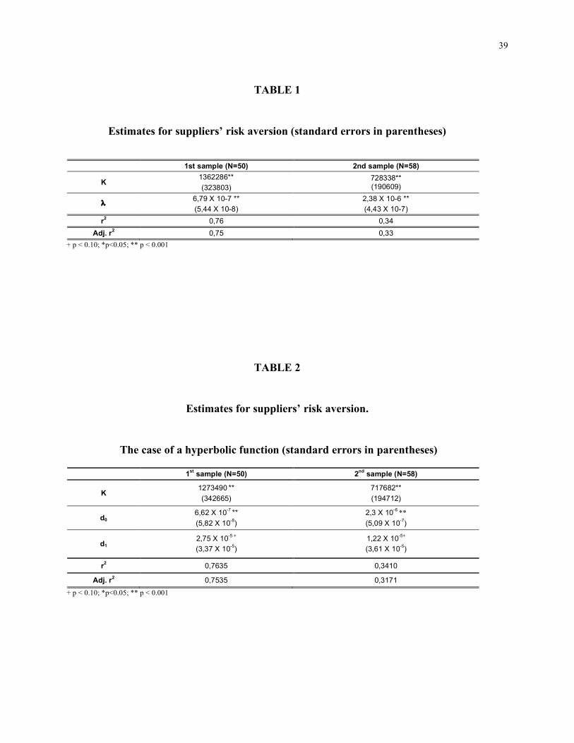
Following Kawasaki and McMillan (1987, 338), we test suppliers’ risk aversion assuming the

existence of a linear relationship between the mean (µ) and variance (s2) of suppliers’ profits:

µ = (½ λ) s2 + k

(½ λ) s2 is the risk premium and k is the residual profit. λ>0 implies that suppliers are risk averse.

We estimate this equation by ordinary least squares (OLS) using samples’ means and variances

of suppliers’ operating income as measures for µ and s2.. Table 1 provides the results of

estimates for suppliers’ risk aversion.

-------------------------------------

Table 1 about here

-------------------------------------

In both samples, λ (suppliers’ risk aversion) is significantly positive17, implying that suppliers are

risk averse.

Furthermore, results in table 1 show that λ of the first sample is considerably lower than λ of the

second sample. This is consistent with the second assumption (large suppliers are less risk averse)

in that the average size of the second sample (194 employees) is considerably larger than the

average size of the first sample (91 employees).

17 In a frictionless market k = 0 (Kawasaki and McMillan, 1987). Instead, in our model k >0 . This can be due to

several reasons. For example, the technological capability necessary to supply high precision AC manufacturers can

constitute a barrier to entry, allowing incumbent suppliers a profit, net of risk premium.

26

As a further test of the second assumption, we follow Asanuma and Kikutani (1992), and

hypothesize a family of functions λ = λ(z), where z represents the size of the firm (number of

employees); the larger is z, the smaller is λ, which is the hypothesis to be tested.

Within this family, we choose one hyperbolic function:

λ = d0 + d1/z

Inserting λ into the mean profit equation µ, we obtain:

µ = (d0 + d1/z) (½ s2) + k

Using suppliers’ data (profits’ means and variances, and number of employees), we estimate d0,

d1 and k. Table 2 shows the results; d0 and d1 and k take significantly positive values for both

samples. These results support both initial hypotheses: a) suppliers are risk averse; and b) large

suppliers are less risk averse. This also implies that the number of employees can be used as a

proxy for risk aversion.

-------------------------------------

Table 2 about here

-------------------------------------

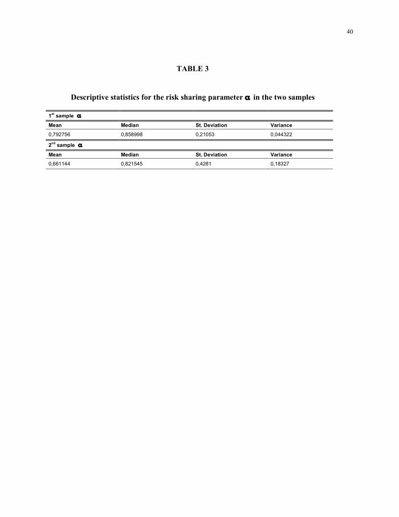
4.2. Risk sharing

Table 3 reports, for both the suppliers’ samples, the descriptive statistics for the risk-sharing

parameter α. Since no international data are available for comparison at the industry level, it is

difficult to assess the degree of risk-sharing going on in the two analyzed cases.

Nonetheless, in both cases, α means and medians are larger than 0.5, values smaller than, but still

comparable with, those found in the auto industry in Japan (Asanuma and Kikutani, 1992), Italy

(Camuffo and Volpato, 1997) and South Korea (Yun, 1999).

27

Indeed, in the Italian high precision AC industry, we would expect much smaller α values than in

the auto industry because: a) an automobile is a much more complex product than a high

precision AC unit; b) first-tier auto suppliers are typically large multinational firms, often

comparable in size to their customers; c) auto OEMs and suppliers, especially in Japan, have a

long history of “voice” practices and stable and cooperative relationships; and d) first tier

suppliers in the Italian high precision AC industry have a diversified customer portfolio and do

not depend on a single customer18. Despite these considerations, α values remain large.

Median values for α are very similar in the two suppliers’ samples, while α mean is larger (and α

variance smaller) in the first than in the second sample. In order to assess if the two

manufacturers absorb risk to different degrees we ran statistical tests for the significance of the

difference between the two suppliers’ population variances and means. We found no statistically

significant difference. Therefore, our data suggest that the two analyzed manufacturers absorb a

similar, nonnegligible degree of risk. We also observe larger α values for suppliers actively

engaged in information sharing, joint improvement efforts and other “voice” practices with their

customers19. These collaborative arrangements derive in part from policies the two buyers have

deliberately adopted, and in part from “district effects” related to geographical proximity, cross-

firm informal and personal ties, customary, albeit tacit, norms of behaviors.

18 The low mean values for SPEC (proportion of the supplier’s sales to a customer to the supplier’s total sales) in

both the samples confirm this. 19 The smaller mean and larger variance of α for suppliers in the second sample suggest that, even though we found

no statistical difference in the means and variances of the two suppliers’ samples, there are differences between the

two manufacturers in terms of purchasing policies and supply network design and management. Our interviews

confirm that the first manufacturer is more advanced in the adoption of “voice” practices in the management of the

supply network.

28

-------------------------------------

Table 3 about here

-------------------------------------

4.3. Determinants of risk sharing

We now turn to testing the agency model and the related research hypothesis. We recall the

buyer’s optimal choice of α:

α= λσ2/(δ + λσ2)

Taking logarithms of both sides of the equation and rearranging, we get:

Ln(1/α– 1) = ln (1/σ2) + ln(1/λ) + lnδ

Where σ2 is the variance of the supplier’s operating costs, λ is the supplier’s risk aversion and δ

is the supplier’s moral hazard. Using the proxies defined in section 3 for λ and δ we obtain the

following model:

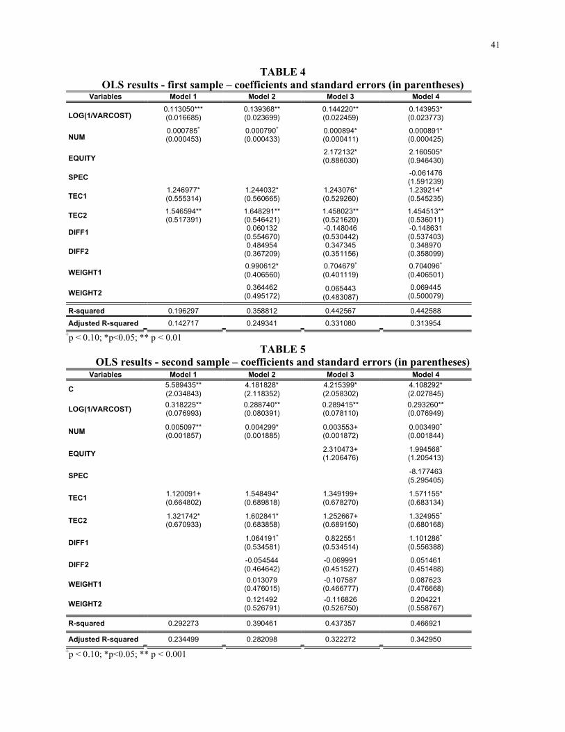
Ln(1/α – 1) = a0 + a1ln (1/VARCOST) + a2NUM + a3EQUITY + a4SPEC + a5TEC1 + a6TEC2 + a7DIFF1 + a8DIFF2 + a9WEIGHT1 + a10WEIGHT2 + ε

Tables 4 and 5 show the results of the OLS analysis for both the suppliers’ samples.

Hypothesis 1 is strongly supported for both the analyzed cases: the larger the supplier’s cost

fluctuations are, the larger is the risk-sharing parameter. Both the analyzed manufacturers are

willing to absorb more risk if cost uncertainty is larger.

29

Also hypothesis 2A is verified for both the samples (p<0.05 and p<0.1)20. The smaller (the more

risk averse) the supplier is, the larger the risk premium it requires and the larger the risk the

manufacturer absorbs (larger α).

As concerns the degree of business concentration (measured by SPEC), even though the

coefficients are negative as predicted, the regression results are not significant (see model 4 in

table 4 and 5). Thus, Hypothesis 2B is not verified. This is probably due to two facts, related to

structural differences between the Japanese auto industry and the Italian high-precision AC

industry: a) the two manufacturers we analyze are not always the main customers of the suppliers

in the samples; b) the proportion of the supplier’s sales to each of the manufacturer to the

supplier’s total sales is small in absolute terms.

Instead, the results of all the models for both the suppliers’ samples strongly support Hypothesis

2C. The more solid is the supplier’s financial structure (lower debt-equity ratio), the lower its

risk aversion, and the smaller is the fraction of risk absorbed by the buyer.

The regression results also show, for both the suppliers’ samples, that the degree of technological

development is negatively related to α. Coefficient signs for TEC1 and TEC2 are always positive

and significant. Therefore, Hypothesis 3A is verified. The larger is the supplier’s degree of

technological development (which is a proxy for moral hazard), the smaller the risk absorbed by

the buyer.

Hypothesis 3B is not verified. After double checking our data, especially the transcripts of the

interviews with the purchasing managers of the two manufacturers, we believe that this can partly

stem form the fact that our measure of the difficulty to find alternative sources is ambiguous and

20 Note that, for this hypothesis to be verified, the sign of the coefficient must be positive, given that the dependent

variable is Ln(1/α – 1).

30

not appropriate to capture moral hazard. Probably, the variable DIFF (the number of suppliers

currently selling the same component) is more the result of the manufacturer’s sourcing strategy

(for example single or double sourcing as opposed to multiple sourcing) than a proxy for a typical

“small numbers” market situation.

Regression results do not support Hypothesis 3C, either. This is probably due to the fact that a

large number of components uniformly contribute to the total manufacturing cost of a high

precision AC unit. Even though many of these components (such as electronic controls) are

complex and important in differentiating the final product and determining its technical

performance and quality, most of them account for less than 1% of the full manufacturing cost of

the final product. Therefore, in this specific industrial setting, the proportion of the component’s

cost to the high precision AC unit’s full manufacturing cost does not discriminate the components

in terms of comparative importance.

-------------------------------------

Table 4 about here

-------------------------------------

-------------------------------------

Table 5 about here

-------------------------------------

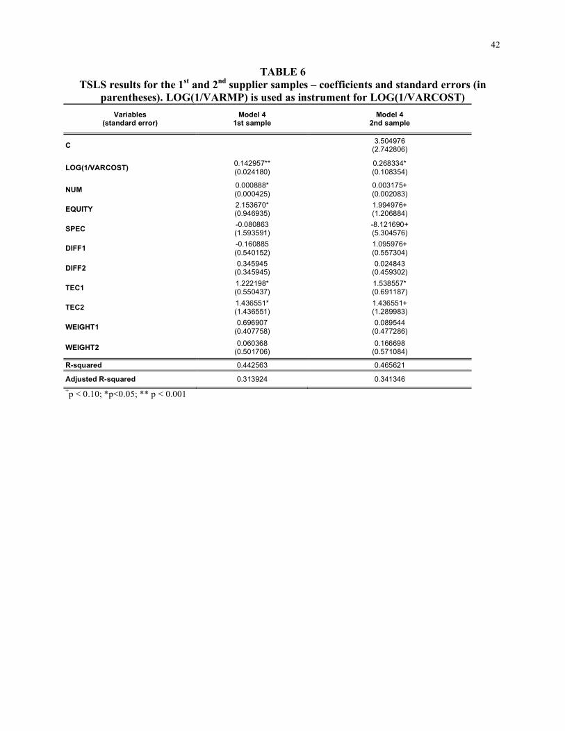
4.4. Residual analysis and model improvement

The models presented in the previous section, as well as those published by Kawasaki and

McMillan (1987), Asanuma and Kikutani (1992), Camuffo and Volpato (1997) and Yun (1999)

are flawed by a problem of endogeneity that we solve in this section.

31

The use of OLS is appropriate when explanatory variables are not correlated to the disturbance

term. An endogeneity problem arises when one or more explanatory variables are correlated to

the disturbance term. In the models presented in the previous section, one explanatory variable

suffers from endogeneity and introduces a measurement error: cost fluctuation (σ2). The

measurement error is introduced into the regressions by both the independent variable - ln(1/σ2) –

and the dependent variable – ln(1/α - 1) - which is a function of the standard deviation of costs

(σ).

We solve this endogeneity problem using TSLS (Two-Stage Least Squares) instead of OLS, i.e.

introducing an instrumental variable as an alternative measure of supplier’s cost fluctuation, the

variance of the cost of raw, subsidiary and expendable materials (VARMP). Noteworthy, the

fluctuations of these costs are mainly exogenously determined. Hence, they represent more

effectively the degree of environmental uncertainty suppliers are faced with.

TSLS results support our hypothesis for both the suppliers’ samples with some improvements in

the sign and significance of the coefficients (table 6).

Finally, we checked the assumption of homoscedasticity of the error term. From a graphic

analysis, the residuals do not appear heteroscedastic. This is the reason why we did not use the

White-adjusted standard errors to calculate the significance of the estimated coefficients.

-------------------------------------

Table 6 about here

-------------------------------------

32

5. Implications

Our microeconometric analyses show that both the analyzed manufacturers absorb risk to a

nonnegligible degree, and, in accordance with agency theory predictions, supports the hypothesis

that buyers absorb more risk a) the bigger are the fluctuations in the supplier’s costs; b) the more

risk averse is the supplier; and c) the less severe is the supplier’s moral hazard. These results are

consistent with other previous studies of this sort, conducted in other industries and countries.

From a research perspective, this study improves previous analysis by: a) testing and verifying a

wider set of hypotheses; b) proposing new proxies for risk aversion and moral hazard; c)

constructing original firm-level databases, mostly on primary and certified data sources, which

provides a more reliable ground for statistical analysis; and d) solving, through the use of TSLS

instead of OLS regression, the problem of endogeneity which affected all previous studies.

This study also offers to practitioners some insights as regards the design of supply contracts, the

optimal allocation of risk across supply chains and the management of supply networks.

Firstly, we suggest that purchasing managers include risk sharing as a conceptual cornerstone in

the design and management of their supply networks. For example, a somehow refined, contract-

specific version of the risk sharing parameter α, calculated for example applying activity based

costing methodologies, could complement vendor rating techniques and become an integrative

part of suppliers’ assessment. In doing that, the economic, financial and technical variables we

use in this study, all readily available at the business level, could constitute a sort of preliminary

template for risk sharing analysis and reporting.

Secondly, some of the findings of this study could be used to complement purchasing and supply

management practices (vendor rating, cost structure analysis, total cost of ownership, target

costing) in supply chain policy making. For example, buyers who wish to engage in the

technological development of small, rapidly evolving suppliers, should be prepared to measure

33

and maneuver risk sharing as the supplier and the corresponding relation evolve. Buyers should

be willing to absorb more risk in the early stage of the supplier relation life-cycle, nurturing and

protecting the target supplier against environmental uncertainty by stabilizing its profits. As the

relation evolves, however, since the supplier’s potential moral hazard increases, they should

become more cautious in risk sharing and invest even more heavily in “voice” practices (to

overcome information asymmetry and build trust). Similarly, the availability of data on how a

buyer has shared the risk with suppliers provides a more solid basis for the design of flexible

supply contracts. For example, performing sensitivity analysis on risk sharing parameters can

lead to more effective price and quantity negotiations in buy back and revenue sharing contracts.

Thirdly, the availability of industry benchmarks for α values would help the parties pursuing the

global optimization of the supply chain, and even provide support to government industrial

policy. For example, buyers could use such data to monitor suppliers’ free riding if suppliers

enjoy some dominant position in the market for a given component. Alternatively, suppliers

could use such data to monitor buyers’ risk sharing policies and avoid exploitation.

Further research along three directions (largely corresponding to three limitations this study

shares with similar, previous ones) would improve the scientific rigor and managerial relevance

of this stream of investigation.

Firstly, the estimation of the risk sharing parameter α remains somewhat problematic (Okamuro,

2001). The fluctuation of supplier’s costs and profits depends on changes not only in unit costs

and prices, but also in quantities. If reliable data on volume variability (and on inventory

variations) were available (but in our case neither buyers nor suppliers were willing or ready to

provide them), it would become possible to distinguish between the volume-related and the cost-

34

related components of risk leading to a more articulated estimate and understanding of risk

allocation in supply chain contracting.

A second conceptual limit also relates to the nature of the risk sharing parameter α. Since α is

calculated using data on operating costs and income from suppliers’ financial reports, it is a

comprehensive measure which refers to all the supplier’s clients and not to a specific customer,

relation and contract. Therefore, α is a characteristic of the supplier and not of a specific buyer-

supplier relation. Given this assumption, the models used so far remain oversimplified, especially

when the supplier’s portfolio of customers is diversified, contractual arrangements change

systematically and buyers’ purchasing philosophy differ significantly. Further research should

address this issue breaking down the analysis by customer, for example calculating, using

sophisticated cost accounting methodologies, contract specific α values, and then modeling risk

allocation at this more disaggregated level of analysis.

Thirdly, the agency model we applied does not clarify the relationship between risk allocation

and the nature of the supplier relation per se. Further evidence of a positive link between

cooperative, stable supplier relations and risk sharing should be sought complementing the model

with variables able to capture such relational aspects as trust or the degree of customer-supplier

integration (Helper and Sako, 1998).

35

References

Anupindi, R., Akella, R., Diversification under supply uncertainty, Management Science, 39:

944-964

Aoki, M., 1988, Information incentives and bargaining structure in the Japanese economy,

Cambridge: MA, Cambridge University Press

Asanuma, B., 1989, Manufacturer-supplier relationships in Japan and the concept of relation-

specific skill, Journal of the Japanese and International Economies, 3:1-30

Asanuma, B., Kikutani, T., 1992, Risk Absorption in Japanese Subcontracting: A

microeconometric study of the automobile industry, Journal of the Japanese and

International Economies, 6: 1-29

Baker, G., Gibbons, R., Murphy, K.J., 2002, Relational Contracts and the Theory of the Firm,

Quarterly Journal of Economics, 2002, 109,112-1156.

Cachon, G.P., 2001, Turning the supply chain into a revenue chain, Harvard Business Review,

79 (3): 20-22

Cachon, G.P., Lariviere, M.A., 2001, Contracting to assure supply: How to share demand

forecasts in a supply chain, Management Science, 47: 629-646

Camuffo, A., Volpato, G., 1997, Nuove forme di integrazione operativa: Il caso della

componentistica automobilistica, Milan: Italy, Franco Angeli.

Chung-Lun, L., Kouvelis, P., 1999, Flexible and risk-sharing supply contracts under price

uncertainty, Management Science, 45: 1378-1399

Cooper, R., Slagmulder, R., 1999, Develop profitable new products with target costing, Sloan

Management Review, 40 (4), 23-34

Cusumano, M.A., Takeishi, A., 1991, Supplier relations and management: a survey of Japanese,

Japanese-transplants, and US auto plants, Strategic Management Journal, 12: 563-588

36

Dawid, H., Kopel, M., 2003, A comparison of exit and voice relationships under common

uncertainty, Journal of Economics & Management Strategy, 12: 531-555

Dyer, J.H., 2000, Collaborative advantage: Winning through extended enterprise supplier

networks, New York: NY, Oxford University Press.

Dyer, J.H., Ouchi W.G., 1993, Japanese-style partnership: Giving companies a competitive edge,

Sloan Management Review, 35(1): 51-84

Dyer, J. H., Chu, W., 2003, The role of trustworthiness in reducing transaction costs and

improving performance: Empirical evidence from the United States, Japan, and Korea,

Organization Science, 14: 57-69

Eisenhardt, K., M., 1989, Agency theory: An assessment and review, Academy of Management

Review, 14: 57-74

Ellram, L. M. (1996), A structured method for applying purchasing cost management tools,

International Journal of Purchasing and Materials Management, 32: 20-28

Ellram, L. M. and Siferd, S. P. (1998), Total cost of ownership: A key concept in strategic cost

management decisions, Journal of Business Logistics, 19: 55-84

Ellram, M.L., Zsidisin, G.A., 2002, An agency theory investigation of supply risk management,

Journal of Supply Chain Management, 39 (3), 15-27

Ferrin, B. G. and Plank, R. E. (2002), Total cost of ownership models: An exploratory study,

Journal of Supply Chain Management, 38 (3): 16-22

Fine, C., 1998, Clock Speed. Winning Industry control in the Age of Temporary Advantage,

Reading: MA, Perseus Books

Gibbons, R., 1997, “An Introduction to Game Theory for Applied Economists, Journal of

Economic Perspectives, 11: 127-149.

37

Helper, S., Sako, M., 1995, Supplier Relations and Management: A survey of Japanese, Japanese-

Transplant, and US auto plants, Sloan Management Review, 36 (3): 77-84

Helper, S., Sako, M., 1998, Determinants of trust in supplier relations: Evidence from the

automotive industry in Japan and the United States”, Journal of Economic Behavior &

Organization, 34: 387-418

Helper, S., MacDuffie, J. P. and Sabel, C. 2000, Pragmatic collaborations: Advancing knowledge

while controlling opportunism, Industrial and Corporate Change, 9: 443-483

Holmstrom, B., Milgrom, P., 1987, Aggregation and linearity in the provision of intertemporal

incentives, Econometrica, 55: 303-328

Kawasaki, S., McMillan J., 1987, The design of contracts: Evidence from the Japanese

subcontracting, Journal of the Japanese and International Economies, 1: 327-349

Levinthal, D., 1988, A survey of agency models of organization, Journal of Economic Behavior

and Organization, 9: 34-45

MacDuffie J.P., Helper S., 1997, Creating lean suppliers: Diffusing lean production through the

supply chain, California Management Review, 39 (4): 118-151

McAfee, R.P., McMillan, J., 1986, Bidding for contracts: A principal-agent analysis, Rand

Journal of Economics, 17: 326-338

Okamuro, H., 2001, Risk sharing in the supplier relationship: New evidence from the Japanese

automotive industry, Journal of Economic Behavior & Organization, 45: 361-382

Shank, J. K., 1999, Target costing as a strategic tool, Sloan Management Review, 41 (1): 73-83

Simchi-Levi, D., Kaminsky, P., Simchi-Levi, E., 2004, Managing the Supply Chain. The

Definitive Guide for the Business Professional, New York: NY, McGraw-Hill.

Tomlin, B., 2003, Capacity investments in supply chains: Sharing the gain rather than sharing the

pain, Manufacturing and Service Operations Management, 5: 317-333

38

Tsay A.A., 1999, The quantity flexibility contract and supplier-customer incentives,

Management Science, 45: 1339-1358

Williamson, O., E., 1975, Markets and Hierarchies: Analysis and Antitrust Implications, New

York: NY, The Free Press.

Yun, M., 1999, Subcontracting relations in the Korean automotive industry: risk sharing and

technological capability, International Journal of Industrial Organization 17: 81–108

39

TABLE 1

Estimates for suppliers’ risk aversion (standard errors in parentheses)

1st sample (N=50) 2nd sample (N=58)

K 1362286** (323803)

728338** (190609)

λ 6,79 X 10-7 ** (5,44 X 10-8)

2,38 X 10-6 ** (4,43 X 10-7)

r2 0,76 0,34 Adj. r2 0,75 0,33

+ p < 0.10; *p<0.05; ** p < 0.001

TABLE 2

Estimates for suppliers’ risk aversion.

The case of a hyperbolic function (standard errors in parentheses)

1st sample (N=50) 2nd sample (N=58)

K 1273490 **

(342665) 717682**

(194712)

d0 6,62 X 10-7 **

(5,82 X 10-8) 2,3 X 10-6 **

(5,09 X 10-7)

d1 2,75 X 10-5 +

(3,37 X 10-5) 1,22 X 10-5+

(3,61 X 10-5)

r2 0,7635 0,3410

Adj. r2 0,7535 0,3171

+ p < 0.10; *p<0.05; ** p < 0.001

40

TABLE 3

Descriptive statistics for the risk sharing parameter α in the two samples

1st sample α

Mean Median St. Deviation Variance

0,792756 0,858998 0,21053 0,044322

2nd sample α

Mean Median St. Deviation Variance

0,661144 0,821545 0,4281 0,18327

41

TABLE 4 OLS results - first sample – coefficients and standard errors (in parentheses)

Variables Model 1 Model 2 Model 3 Model 4

LOG(1/VARCOST) 0.113050*** (0.016685)

0.139368** (0.023699)

0.144220** (0.022459)

0.143953* (0.023773)

NUM 0.000785+ (0.000453)

0.000790+ (0.000433)

0.000894* (0.000411)

0.000891* (0.000425)

EQUITY 2.172132*

(0.886030) 2.160505* (0.946430)

SPEC -0.061476 (1.591239)

TEC1 1.246977* (0.555314)

1.244032* (0.560665)

1.243076* (0.529260)

1.239214* (0.545235)

TEC2 1.546594** (0.517391)

1.648291** (0.546421)

1.458023** (0.521620)

1.454513** (0.536011)

DIFF1 0.060132 (0.554670)

-0.148046 (0.530442)

-0.148631 (0.537403)

DIFF2 0.484954

(0.367209) 0.347345

(0.351156) 0.348970

(0.358099)

WEIGHT1 0.990612*

(0.406560) 0.704679+ (0.401119)

0.704096+ (0.406501)

WEIGHT2 0.364462

(0.495172) 0.065443

(0.483087) 0.069445

(0.500079)

R-squared 0.196297 0.358812 0.442567 0.442588

Adjusted R-squared 0.142717 0.249341 0.331080 0.313954 +p < 0.10; *p<0.05; ** p < 0.01

TABLE 5 OLS results - second sample – coefficients and standard errors (in parentheses)

Variables Model 1 Model 2 Model 3 Model 4

C 5.589435** (2.034843)

4.181828* (2.118352)

4.215399* (2.058302)

4.108292* (2.027845)

LOG(1/VARCOST) 0.318225** (0.076993)

0.288740** (0.080391)

0.289415** (0.078110)

0.293260** (0.076949)

NUM 0.005097** (0.001857)

0.004299* (0.001885)

0.003553+ (0.001872)

0.003490+

(0.001844)

EQUITY 2.310473+ (1.206476)

1.994568+

(1.205413)

SPEC -8.177463 (5.295405)

TEC1 1.120091+ (0.664802)

1.548494* (0.689818)

1.349199+ (0.678270)

1.571155* (0.683134)

TEC2 1.321742* (0.670933)

1.602841* (0.683858)

1.252667+ (0.689150)

1.324955+

(0.680168)

DIFF1 1.064191+

(0.534581) 0.822551

(0.534514) 1.101286+

(0.556388)

DIFF2 -0.054544

(0.464642) -0.069991 (0.451527)

0.051461 (0.451488)

WEIGHT1 0.013079 (0.476015)

-0.107587 (0.466777)

0.087623 (0.476668)

WEIGHT2 0.121492

(0.526791) -0.116826 (0.526750)

0.204221 (0.558767)

R-squared 0.292273 0.390461 0.437357 0.466921

Adjusted R-squared 0.234499 0.282098 0.322272 0.342950 +p < 0.10; *p<0.05; ** p < 0.001

42

TABLE 6 TSLS results for the 1st and 2nd supplier samples – coefficients and standard errors (in

parentheses). LOG(1/VARMP) is used as instrument for LOG(1/VARCOST) Variables

(standard error) Model 4

1st sample Model 4

2nd sample

C 3.504976 (2.742806)

LOG(1/VARCOST) 0.142957** (0.024180)

0.268334* (0.108354)

NUM 0.000888* (0.000425)

0.003175+ (0.002083)

EQUITY 2.153670* (0.946935)

1.994976+ (1.206884)

SPEC -0.080863 (1.593591)

-8.121690+ (5.304576)

DIFF1 -0.160885 (0.540152)

1.095976+ (0.557304)

DIFF2 0.345945 (0.345945)

0.024843 (0.459302)

TEC1 1.222198* (0.550437)

1.538557* (0.691187)

TEC2 1.436551* (1.436551)

1.436551+ (1.289983)

WEIGHT1 0.696907 (0.407758)

0.089544 (0.477286)

WEIGHT2 0.060368 (0.501706)

0.166698 (0.571084)

R-squared 0.442563 0.465621

Adjusted R-squared 0.313924 0.341346 +p < 0.10; *p<0.05; ** p < 0.001