RiskPremia: AsymmetricTail Risks andExcessReturns arXiv ... · theoretical prices, as it allows one to introduce an extra ﬁtting parameter conveniently called the ... (CARA) utility

arX

iv:1

409.

7720

v3 [

q-fi

n.G

N]

30

Oct

201

5November 2, 2015 Quantitative Finance risk˙premium˙Rev˙QF

To appear in Quantitative Finance, Vol. 00, No. 00, Month 20XX, 1–22

Risk Premia:

Asymmetric Tail Risks and Excess Returns

Y. Lemperiere, C. Deremble, T. T. Nguyen

P. Seager, M. Potters, J. P. Bouchaud

Capital Fund Management,

23 rue de l’Universite, 75007 Paris, France

(Received 00 Month 20XX; in final form 00 Month 20XX)

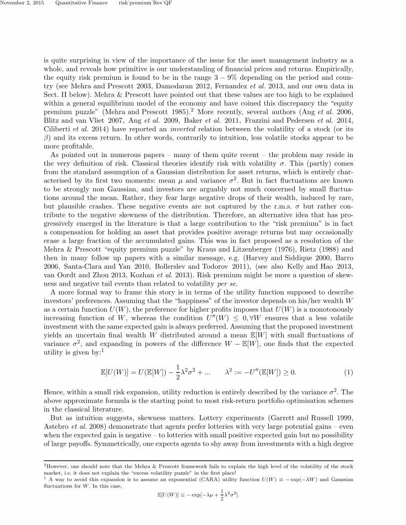
We present extensive evidence that “risk premium” is strongly correlated with tail-risk skewness but verylittle with volatility. We introduce a new, intuitive definition of skewness and elicit an approximatelylinear relation between the Sharpe ratio of various risk premium strategies (Equity, Fama-French, FXCarry, Short Vol, Bonds, Credit) and their negative skewness. We find a clear exception to this rule: trendfollowing has both positive skewness and positive excess returns. This is also true, albeit less markedly, ofthe Fama-French “Value” factor and of the “Low Volatility” strategy. This suggests that some strategiesare not risk premia but genuine market anomalies. Based on our results, we propose an objective criterionto assess the quality of a risk-premium portfolio.

Keywords: Alternative Investments, Asymmetry, Economics of Risk, Empirical Time Series Analysis,Hedge Funds, Market Anomalies.

1. Introduction

One of the pillars of modern finance theory is the concept of “risk premium”, i.e. that a morerisky investment should, on the long run, also be more profitable. The argument leading to sucha conclusion looks, at least at first sight, rock solid: given the choice between two assets with thesame expected return, any rational investor should prefer the less risky one. The resulting smallerdemand for riskier assets should make their prices drop, and therefore their yields go up, until theybecome attractive enough to lure in investors in spite of their higher risk. This simple idea appearsto explain why stock indices on the long run yield higher returns than monetary funds, for example.It is also at the heart of the well-known Capital Asset Pricing Model (CAPM), which predicts thatthe excess return of a given stock (over the risk free rate) is proportional to its so-called “β”, i.e.to its covariance with the market risk (Sharpe 1964).The idea has become so pervasive that its logic has actually inverted: efficient market theorists

assume that any return in excess of the risk free rate should in fact be associated with a non-diversifiable risk factor of some sort – sometimes argued to be unobservable or “latent”. It isoften invoked to do away with any market anomaly or discrepancies between market prices andtheoretical prices, as it allows one to introduce an extra fitting parameter conveniently called the“market price of risk”. 1

Although the argument underlying the existence of risk premia is cogent, estimating and ratio-nalising their order of magnitude in financial markets is still very much a matter of debate. This

1In the context of option pricing, see e.g. (Fouque et al. 2011). Note, however, that since the market price of risk itself is usuallyfound to be strongly fluctuating in time, the predictive strength of these theories becomes frustratingly close to zero.

http://arxiv.org/abs/1409.7720v3

November 2, 2015 Quantitative Finance risk˙premium˙Rev˙QF

is quite surprising in view of the importance of the issue for the asset management industry as awhole, and reveals how primitive is our understanding of financial prices and returns. Empirically,the equity risk premium is found to be in the range 3 − 9% depending on the period and coun-try (see Mehra and Prescott 2003, Damodaran 2012, Fernandez et al. 2013, and our own data inSect. II below). Mehra & Prescott have pointed out that these values are too high to be explainedwithin a general equilibrium model of the economy and have coined this discrepancy the “equitypremium puzzle” (Mehra and Prescott 1985).2 More recently, several authors (Ang et al. 2006,Blitz and van Vliet 2007, Ang et al. 2009, Baker et al. 2011, Frazzini and Pedersen et al. 2014,Ciliberti et al. 2014) have reported an inverted relation between the volatility of a stock (or itsβ) and its excess return. In other words, contrarily to intuition, less volatile stocks appear to bemore profitable.As pointed out in numerous papers – many of them quite recent – the problem may reside in

the very definition of risk. Classical theories identify risk with volatility σ. This (partly) comesfrom the standard assumption of a Gaussian distribution for asset returns, which is entirely char-acterised by its first two moments: mean µ and variance σ2. But in fact fluctuations are knownto be strongly non Gaussian, and investors are arguably not much concerned by small fluctua-tions around the mean. Rather, they fear large negative drops of their wealth, induced by rare,but plausible crashes. These negative events are not captured by the r.m.s. σ but rather con-tribute to the negative skewness of the distribution. Therefore, an alternative idea that has pro-gressively emerged in the literature is that a large contribution to the “risk premium” is in facta compensation for holding an asset that provides positive average returns but may occasionallyerase a large fraction of the accumulated gains. This was in fact proposed as a resolution of theMehra & Prescott “equity premium puzzle” by Kraus and Litzenberger (1976), Rietz (1988) andthen in many follow up papers with a similar message, e.g. (Harvey and Siddique 2000, Barro2006, Santa-Clara and Yan 2010, Bollerslev and Todorov 2011), (see also Kelly and Hao 2013,van Oordt and Zhou 2013, Kozhan et al. 2013). Risk premium might be more a question of skew-ness and negative tail events than related to volatility per se.A more formal way to frame this story is in terms of the utility function supposed to describe

investors’ preferences. Assuming that the “happiness” of the investor depends on his/her wealth Was a certain function U(W ), the preference for higher profits imposes that U(W ) is a monotonouslyincreasing function of W , whereas the condition U ′′(W ) ≤ 0,∀W ensures that a less volatileinvestment with the same expected gain is always preferred. Assuming that the proposed investmentyields an uncertain final wealth W distributed around a mean E[W ] with small fluctuations ofvariance σ2, and expanding in powers of the difference W − E[W ], one finds that the expectedutility is given by:1

E[U(W )] = U(E[W ])− 1

2λ2σ2 + ... λ2 := −U ′′(E[W ]) ≥ 0. (1)

Hence, within a small risk expansion, utility reduction is entirely described by the variance σ2. Theabove approximate formula is the starting point to most risk-return portfolio optimisation schemesin the classical literature.But as intuition suggests, skewness matters. Lottery experiments (Garrett and Russell 1999,

Astebro et al. 2008) demonstrate that agents prefer lotteries with very large potential gains – evenwhen the expected gain is negative – to lotteries with small positive expected gain but no possibilityof large payoffs. Symmetrically, one expects agents to shy away from investments with a high degree

2However, one should note that the Mehra & Prescott framework fails to explain the high level of the volatility of the stockmarket, i.e. it does not explain the “excess volatility puzzle” in the first place!1 A way to avoid this expansion is to assume an exponential (CARA) utility function U(W ) ≡ − exp(−λW ) and Gaussianfluctuations for W . In this case,

E[U(W )] ≡ − exp[−λµ+1

2λ2σ2].


of negative skewness. Clearly, this cannot be captured by Eq. (1) above where skewness is absent; itmay well be the case that the whole concept of utility is anyway insufficient to account for behavioralbiases, see (Kahneman and Tversky 1979). Still, a large number of papers have therefore beendevoted to generalising Markowitz’s portfolio optimisation and the CAPM to account for skewnesspreferences (Kraus and Litzenberger 1976, Harvey and Siddique 2000, Athayde and Flores 2004,Harvey et al. 2010). In terms of utility functions, one can show that the additional conditionU ′′′(W ) ≥ 0,∀W ensures that more positively skewed investments are preferred (Chiu 2010). 2

Our work is clearly in the wake of the above mentioned literature on skewness preferences and tail-risk aversion. We will present extensive evidence that “risk premium” is indeed strongly correlatedwith the skewness of a strategy but very little with its volatility, not only in the equity world – aswas emphasised by previous authors – but in other sectors as well. We will investigate in detail manyclassical so-called “risk premium” strategies (in equities, bonds, currencies, options and credit) andelicit a linear relation between the Sharpe ratio of these strategies and their negative skewness. Wewill find however that some well-known strategies, such as trend following and to a lesser extentthe Fama-French “High minus Low” factor and the “Low Vol” strategy, are clearly not followingthis rule, suggesting that these strategies are not risk premia but genuine market anomalies.Compared to the previous abundant literature, the present results are new in different respects.

First, at variance with most previous investigations (that mostly focusses on stock markets), we donot attempt to frame our empirical analysis within the constraining framework of asset pricing andportfolio theory, but rather let the data speak for itself. This is specially important when studying,as we do here, risk premia across a much larger universe of assets, where the notion of a global“risk factor” (generalizing the market factor in the equity space) is far from clear, as we discussin Sect. 8 below. Second, we introduce a simple way to plot the returns of a portfolio that revealsits skewness to the “naked eye” and suggests an intuitive and robust definition of skewness that ismuch less sensitive to extreme events. Third, our empirical conclusion that for a wide spectrum of“risk premia” strategies, skewness rather than volatility is a determinant of returns is, to the bestof our knowledge, new, as is the finding that some investment strategies – like trend following –seem to behave quite differently.We first start in Sect. 2 with the equity market as a whole and revisit the equity risk premium

world-wide, and its (negative) correlation with the volatility. We then introduce our new, intuitivedefinition of skewness that we use throughout the paper and that we justify in the Appendix. Wefocus on the Fama-French factors in Sect. 3 and study the statistics of market neutral portfolios,including a “Low Volatility” portfolio. We move on to the fixed income world (Sect. 4), where weagain build neutral portfolios. Sect. 5 is devoted to an account of risk premia on currencies (theso-called “Carry Trade”), and finally, in Sect. 6, to the paradigmatic case of selling options. Wesummarise our findings in Sect. 7 with a suggestive linear relation between the Sharpe ratio and theskewness of all the Risk Premium strategies investigated in the paper, and discuss some exceptionsto the rule – i.e. positive Sharpe strategies with zero or positive skewness – that we define as “pureα” strategies. We then end the paper in Sect. 8 by comparing our results to the extended CAPMframework a la Kraus and Litzenberger (1976), Harvey and Siddique (2000). We propose insteada simple argument to rationalise for the Sharpe ratio/skewness trade-off and an objective criterionto assess the quality of a risk premium portfolio.

2More precisely, this preference ordering requires in general the distributions to be “skewness comparable”, which means thattheir cumulative functions must cross twice and only twice (Oja 1981, Chiu 2010). This turns out to be often the case infinancial applications, see below and Appendix.


2. Back to Basics: Risk Premium in Global Equity Markets, and a new definition of

Skewness

2.1. No “volatility premium” in stock indices

According to the standard framework described in the previous section, investing in the stockmarket rather than in risk-free instruments only makes sense if stocks provide, in the long run,better returns than the risk-free rate. The existence and the strength of this equity risk premium(ERP) has been much debated amongst both the academic community and the asset manage-ment industry. The general consensus (confirmed below) is that this premium exists and is in therange 3−9%, with large fluctuations, both across epochs and countries (Mehra and Prescott 2003,Damodaran 2012, Fernandez et al. 2013). Within a classical general equilibrium framework, thispremium appears to be too large. With such a level of ERP, rational investors should put moneymore massively in equities, and the demand for bonds should be much weaker than what we ob-serve, which should lead to a smaller risk premium. This is the “equity premium puzzle” broughtto the fore by Mehra and Prescott (1985).In order to estimate the ERP, it is customary to compute the total return of indices (dividend

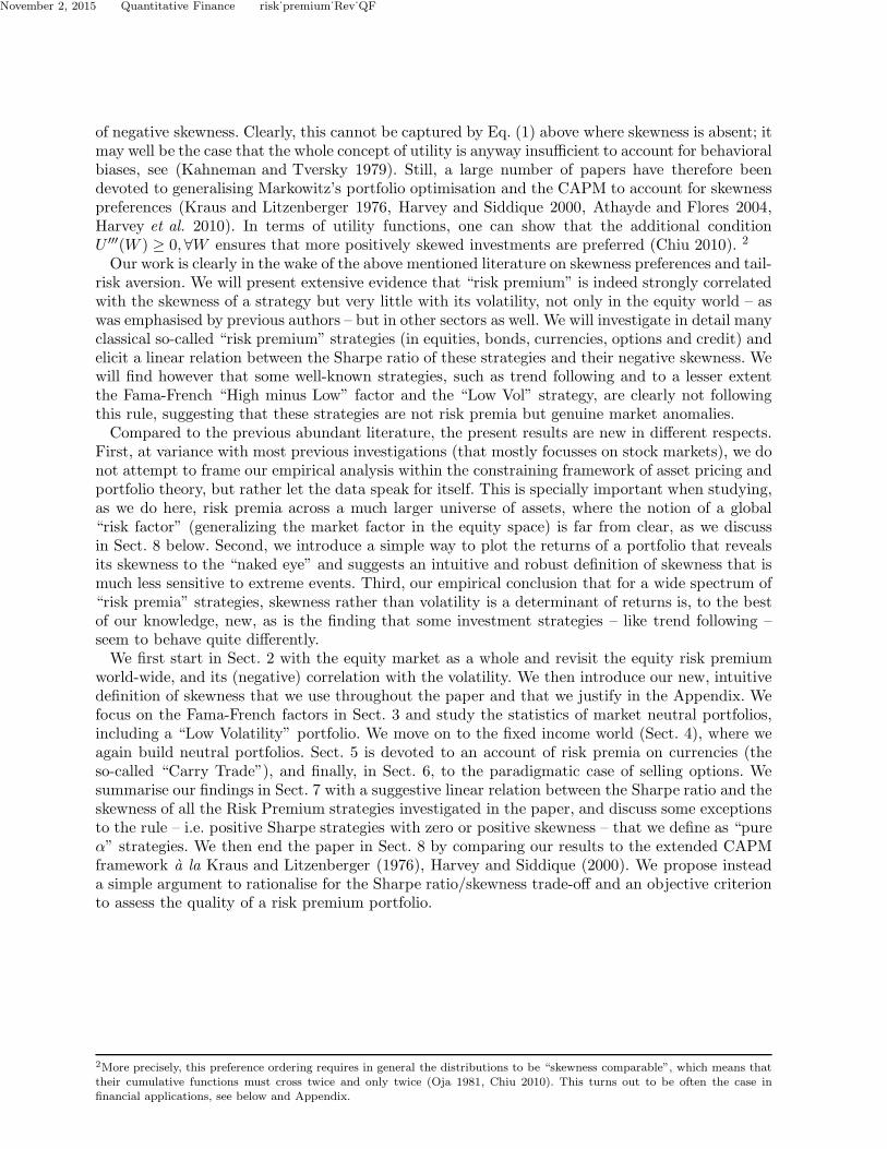
included), and to subtract the risk-free rate. 1 We have therefore computed this cumulated differencefor various countries, using the 10Y government rate as a risk-free asset (using 3-month bills wouldonly give a more flattering result, since short rates are usually lower than 10Y rates). The resultis, as expected, overwhelmingly in favour of the existence of a risk premium, as can be seen fromTable 1 and Fig. 1. All countries but one display positive excess return on the long run (some timeseries go back as far as 1870). The global t-stat of a strategy equi-invested in all available indicesat any moment in time is 4.2. The average value (weighted by the number of available years foreach country) is found to be ≈ 5% with a cross-sectional dispersion of ±3%, compatible with thenumbers quoted above (Mehra and Prescott 2003, Damodaran 2012, Fernandez et al. 2013).In the fourth column of Table 1, we give the average annual volatility of the corresponding index.

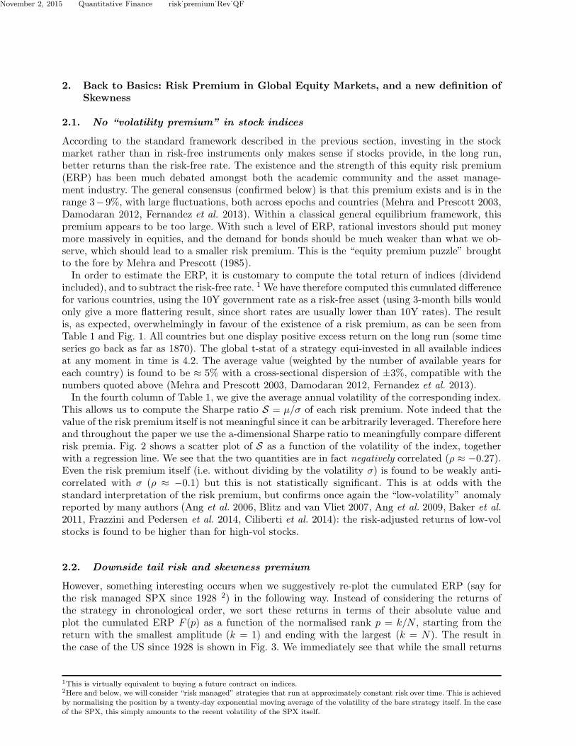
This allows us to compute the Sharpe ratio S = µ/σ of each risk premium. Note indeed that thevalue of the risk premium itself is not meaningful since it can be arbitrarily leveraged. Therefore hereand throughout the paper we use the a-dimensional Sharpe ratio to meaningfully compare differentrisk premia. Fig. 2 shows a scatter plot of S as a function of the volatility of the index, togetherwith a regression line. We see that the two quantities are in fact negatively correlated (ρ ≈ −0.27).Even the risk premium itself (i.e. without dividing by the volatility σ) is found to be weakly anti-correlated with σ (ρ ≈ −0.1) but this is not statistically significant. This is at odds with thestandard interpretation of the risk premium, but confirms once again the “low-volatility” anomalyreported by many authors (Ang et al. 2006, Blitz and van Vliet 2007, Ang et al. 2009, Baker et al.2011, Frazzini and Pedersen et al. 2014, Ciliberti et al. 2014): the risk-adjusted returns of low-volstocks is found to be higher than for high-vol stocks.

2.2. Downside tail risk and skewness premium

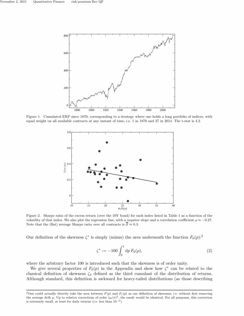
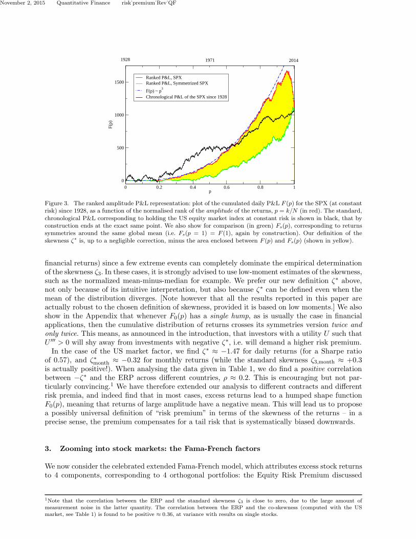
However, something interesting occurs when we suggestively re-plot the cumulated ERP (say forthe risk managed SPX since 1928 2) in the following way. Instead of considering the returns ofthe strategy in chronological order, we sort these returns in terms of their absolute value andplot the cumulated ERP F (p) as a function of the normalised rank p = k/N , starting from thereturn with the smallest amplitude (k = 1) and ending with the largest (k = N). The result inthe case of the US since 1928 is shown in Fig. 3. We immediately see that while the small returns

1This is virtually equivalent to buying a future contract on indices.2Here and below, we will consider “risk managed” strategies that run at approximately constant risk over time. This is achievedby normalising the position by a twenty-day exponential moving average of the volatility of the bare strategy itself. In the caseof the SPX, this simply amounts to the recent volatility of the SPX itself.


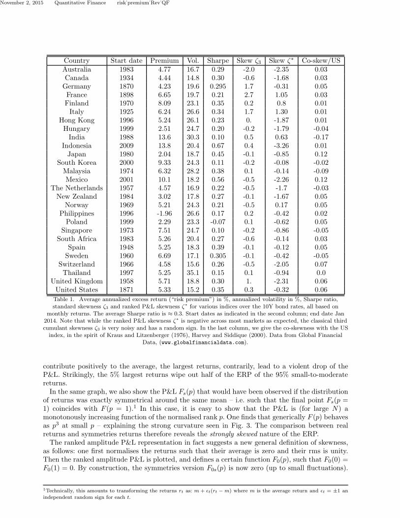
Country Start date Premium Vol. Sharpe Skew ζ3 Skew ζ∗ Co-skew/USAustralia 1983 4.77 16.7 0.29 -2.0 -2.35 0.03Canada 1934 4.44 14.8 0.30 -0.6 -1.68 0.03Germany 1870 4.23 19.6 0.295 1.7 -0.31 0.05France 1898 6.65 19.7 0.21 2.7 1.05 0.03Finland 1970 8.09 23.1 0.35 0.2 0.8 0.01Italy 1925 6.24 26.6 0.34 1.7 1.30 0.01

Hong Kong 1996 5.24 26.1 0.23 0. -1.87 0.01Hungary 1999 2.51 24.7 0.20 -0.2 -1.79 -0.04India 1988 13.6 30.3 0.10 0.5 0.63 -0.17

Indonesia 2009 13.8 20.4 0.67 0.4 -3.26 0.01Japan 1980 2.04 18.7 0.45 -0.1 -0.85 0.12

South Korea 2000 9.33 24.3 0.11 -0.2 -0.08 -0.02Malaysia 1974 6.32 28.2 0.38 0.1 -0.14 -0.09Mexico 2001 10.1 18.2 0.56 -0.5 -2.26 0.12

The Netherlands 1957 4.57 16.9 0.22 -0.5 -1.7 -0.03New Zealand 1984 3.02 17.8 0.27 -0.1 -1.67 0.05

Norway 1969 5.21 24.3 0.21 -0.5 0.17 0.05Philippines 1996 -1.96 26.6 0.17 0.2 -0.42 0.02Poland 1999 2.29 23.3 -0.07 0.1 -0.62 0.05

Singapore 1973 7.51 24.7 0.10 -0.2 -0.86 -0.05South Africa 1983 5.26 20.4 0.27 -0.6 -0.14 0.03

Spain 1948 5.25 18.3 0.39 -0.1 -0.12 0.05Sweden 1960 6.69 17.1 0.305 -0.1 -0.42 -0.05

Switzerland 1966 4.58 15.6 0.26 -0.5 -2.05 0.07Thailand 1997 5.25 35.1 0.15 0.1 -0.94 0.0

United Kingdom 1958 5.71 18.8 0.30 1. -2.31 0.06United States 1871 5.33 15.2 0.35 0.3 -0.32 0.06

Table 1. Average annualized excess return (“risk premium”) in %, annualized volatility in %, Sharpe ratio,standard skewness ζ3 and ranked P&L skewness ζ∗ for various indices over the 10Y bond rates, all based on

monthly returns. The average Sharpe ratio is ≈ 0.3. Start dates as indicated in the second column; end date Jan2014. Note that while the ranked P&L skewness ζ∗ is negative across most markets as expected, the classical thirdcumulant skewness ζ3 is very noisy and has a random sign. In the last column, we give the co-skewness with the USindex, in the spirit of Kraus and Litzenberger (1976), Harvey and Siddique (2000). Data from Global Financial

Data, (www.globalfinancialdata.com).

contribute positively to the average, the largest returns, contrarily, lead to a violent drop of theP&L. Strikingly, the 5% largest returns wipe out half of the ERP of the 95% small-to-moderatereturns.In the same graph, we also show the P&L Fs(p) that would have been observed if the distribution

of returns was exactly symmetrical around the same mean – i.e. such that the final point Fs(p =1) coincides with F (p = 1).1 In this case, it is easy to show that the P&L is (for large N) amonotonously increasing function of the normalised rank p. One finds that generically F (p) behavesas p3 at small p – explaining the strong curvature seen in Fig. 3. The comparison between realreturns and symmetries returns therefore reveals the strongly skewed nature of the ERP.The ranked amplitude P&L representation in fact suggests a new general definition of skewness,

as follows: one first normalises the returns such that their average is zero and their rms is unity.Then the ranked amplitude P&L is plotted, and defines a certain function F0(p), such that F0(0) =F0(1) = 0. By construction, the symmetries version F0s(p) is now zero (up to small fluctuations).

1Technically, this amounts to transforming the returns rt as: m + ǫt(rt − m) where m is the average return and ǫt = ±1 anindependent random sign for each t.


1880 1900 1920 1940 1960 1980 2000

0

200

400

600

800

Figure 1. Cumulated ERP since 1870, corresponding to a strategy where one holds a long portfolio of indices, withequal weight on all available contracts at any instant of time, i.e. 1 in 1870 and 27 in 2014. The t-stat is 4.2.

10 15 20 25 30 35 40σ (%/y)

0

0.2

0.4

0.6

0.8

Sharpe

Figure 2. Sharpe ratio of the excess return (over the 10Y bond) for each index listed in Table 1 as a function of thevolatility of that index. We also plot the regression line, with a negative slope and a correlation coefficient ρ ≈ −0.27.Note that the (flat) average Sharpe ratio over all contracts is S ≈ 0.3.

Our definition of the skewness ζ∗ is simply (minus) the area underneath the function F0(p):2

ζ∗ := −100

∫ 1

0dpF0(p), (2)

where the arbitrary factor 100 is introduced such that the skewness is of order unity.We give several properties of F0(p) in the Appendix and show how ζ∗ can be related to the

classical definition of skewness ζ3 defined as the third cumulant of the distribution of returns.Although standard, this definition is awkward for heavy-tailed distributions (as those describing

2One could actually directly take the area between F (p) and Fs(p) as our definition of skewness, i.e. without first removingthe average drift µ. Up to relative corrections of order (µ/σ)2 , the result would be identical. For all purposes, this correctionis extremely small, at least for daily returns (i.e. less than 10−3).


0 0.2 0.4 0.6 0.8 1p

0

500

1000

1500

F(p)

Ranked P&L, SPX Ranked P&L, Symmetrized SPX

F(p) ~ p3

Chronological P&L of the SPX since 1928

1928 1971 2014

Figure 3. The ranked amplitude P&L representation: plot of the cumulated daily P&L F (p) for the SPX (at constantrisk) since 1928, as a function of the normalised rank of the amplitude of the returns, p = k/N (in red). The standard,chronological P&L corresponding to holding the US equity market index at constant risk is shown in black, that byconstruction ends at the exact same point. We also show for comparison (in green) Fs(p), corresponding to returnssymmetries around the same global mean (i.e. Fs(p = 1) = F (1), again by construction). Our definition of theskewness ζ∗ is, up to a negligible correction, minus the area enclosed between F (p) and Fs(p) (shown in yellow).

financial returns) since a few extreme events can completely dominate the empirical determinationof the skewness ζ3. In these cases, it is strongly advised to use low-moment estimates of the skewness,such as the normalized mean-minus-median for example. We prefer our new definition ζ∗ above,not only because of its intuitive interpretation, but also because ζ∗ can be defined even when themean of the distribution diverges. [Note however that all the results reported in this paper areactually robust to the chosen definition of skewness, provided it is based on low moments.] We alsoshow in the Appendix that whenever F0(p) has a single hump, as is usually the case in financialapplications, then the cumulative distribution of returns crosses its symmetries version twice andonly twice. This means, as announced in the introduction, that investors with a utility U such thatU ′′′ > 0 will shy away from investments with negative ζ∗, i.e. will demand a higher risk premium.In the case of the US market factor, we find ζ∗ ≈ −1.47 for daily returns (for a Sharpe ratio

of 0.57), and ζ∗month ≈ −0.32 for monthly returns (while the standard skewness ζ3,month ≈ +0.3is actually positive!). When analysing the data given in Table 1, we do find a positive correlationbetween −ζ∗ and the ERP across different countries, ρ ≈ 0.2. This is encouraging but not par-ticularly convincing.1 We have therefore extended our analysis to different contracts and differentrisk premia, and indeed find that in most cases, excess returns lead to a humped shape functionF0(p), meaning that returns of large amplitude have a negative mean. This will lead us to proposea possibly universal definition of “risk premium” in terms of the skewness of the returns – in aprecise sense, the premium compensates for a tail risk that is systematically biased downwards.

3. Zooming into stock markets: the Fama-French factors

We now consider the celebrated extended Fama-French model, which attributes excess stock returnsto 4 components, corresponding to 4 orthogonal portfolios: the Equity Risk Premium discussed

1Note that the correlation between the ERP and the standard skewness ζ3 is close to zero, due to the large amount ofmeasurement noise in the latter quantity. The correlation between the ERP and the co-skewness (computed with the USmarket, see Table 1) is found to be positive ≈ 0.36, at variance with results on single stocks.


above (i.e. market minus the risk-free rate, MKT), SMB (“Small” caps minus “Big” caps), UMD(“Up” – previous winners minus “Down” – previous losers) and HML (High book to price – “value”stocks minus Low book to price – “growth” stocks), each of which is interpreted as a reward for aspecific risk, even if the origin of said risk is not always clear.The first, long market portfolio is tautologically not market neutral, while the other three are

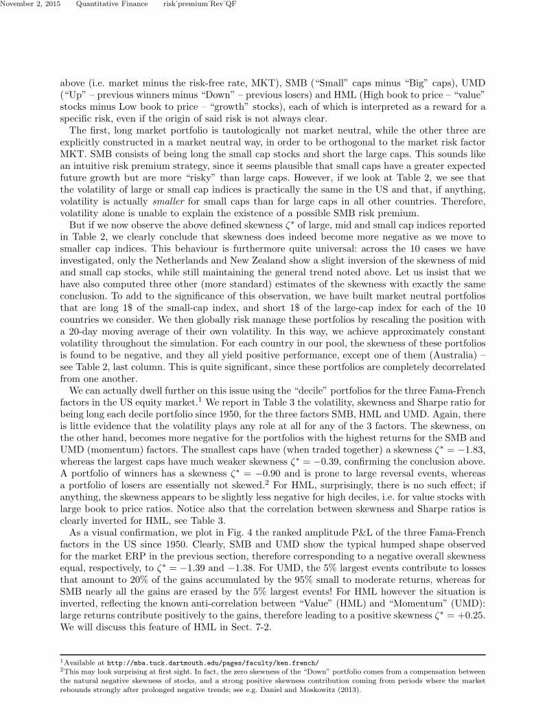
explicitly constructed in a market neutral way, in order to be orthogonal to the market risk factorMKT. SMB consists of being long the small cap stocks and short the large caps. This sounds likean intuitive risk premium strategy, since it seems plausible that small caps have a greater expectedfuture growth but are more “risky” than large caps. However, if we look at Table 2, we see thatthe volatility of large or small cap indices is practically the same in the US and that, if anything,volatility is actually smaller for small caps than for large caps in all other countries. Therefore,volatility alone is unable to explain the existence of a possible SMB risk premium.But if we now observe the above defined skewness ζ∗ of large, mid and small cap indices reported

in Table 2, we clearly conclude that skewness does indeed become more negative as we move tosmaller cap indices. This behaviour is furthermore quite universal: across the 10 cases we haveinvestigated, only the Netherlands and New Zealand show a slight inversion of the skewness of midand small cap stocks, while still maintaining the general trend noted above. Let us insist that wehave also computed three other (more standard) estimates of the skewness with exactly the sameconclusion. To add to the significance of this observation, we have built market neutral portfoliosthat are long 1$ of the small-cap index, and short 1$ of the large-cap index for each of the 10countries we consider. We then globally risk manage these portfolios by rescaling the position witha 20-day moving average of their own volatility. In this way, we achieve approximately constantvolatility throughout the simulation. For each country in our pool, the skewness of these portfoliosis found to be negative, and they all yield positive performance, except one of them (Australia) –see Table 2, last column. This is quite significant, since these portfolios are completely decorrelatedfrom one another.We can actually dwell further on this issue using the “decile” portfolios for the three Fama-French

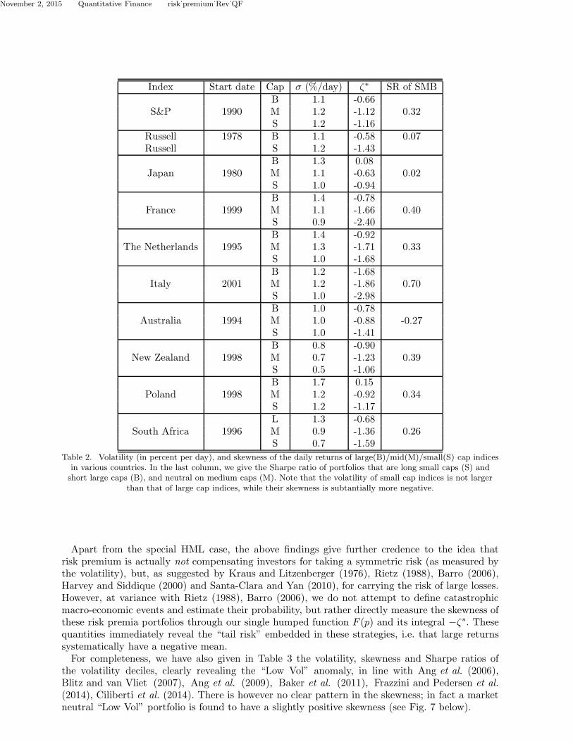
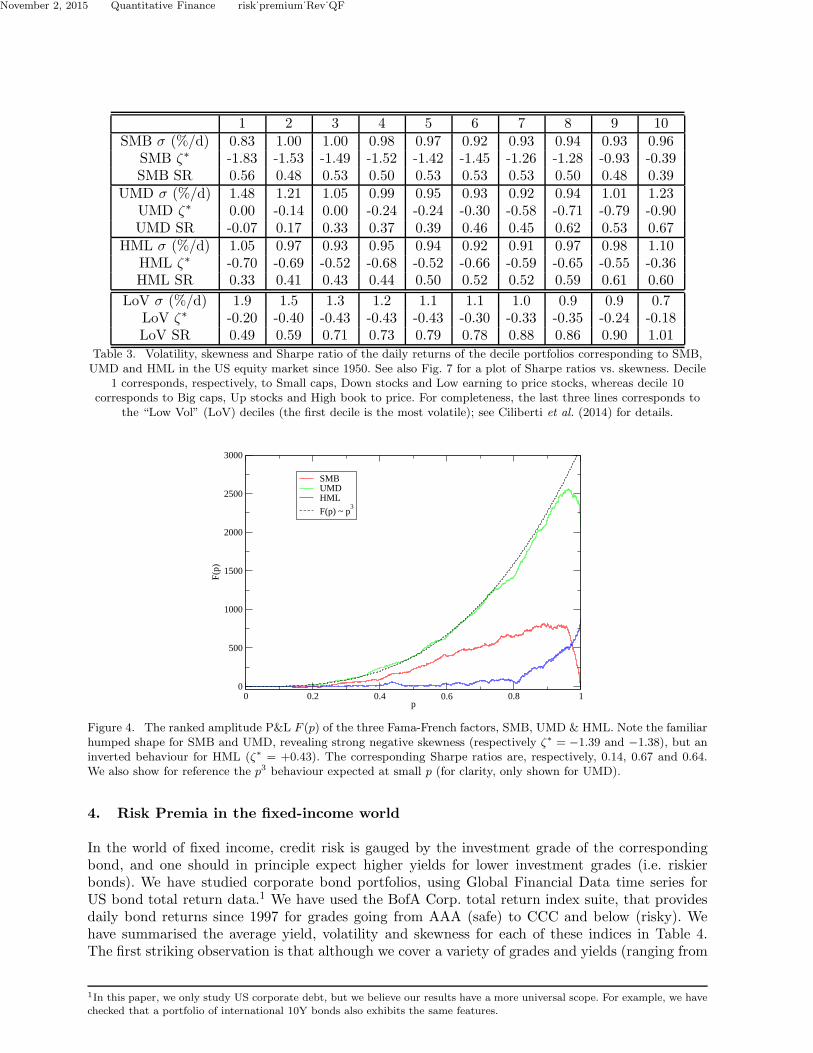
factors in the US equity market.1 We report in Table 3 the volatility, skewness and Sharpe ratio forbeing long each decile portfolio since 1950, for the three factors SMB, HML and UMD. Again, thereis little evidence that the volatility plays any role at all for any of the 3 factors. The skewness, onthe other hand, becomes more negative for the portfolios with the highest returns for the SMB andUMD (momentum) factors. The smallest caps have (when traded together) a skewness ζ∗ = −1.83,whereas the largest caps have much weaker skewness ζ∗ = −0.39, confirming the conclusion above.A portfolio of winners has a skewness ζ∗ = −0.90 and is prone to large reversal events, whereasa portfolio of losers are essentially not skewed.2 For HML, surprisingly, there is no such effect; ifanything, the skewness appears to be slightly less negative for high deciles, i.e. for value stocks withlarge book to price ratios. Notice also that the correlation between skewness and Sharpe ratios isclearly inverted for HML, see Table 3.As a visual confirmation, we plot in Fig. 4 the ranked amplitude P&L of the three Fama-French

factors in the US since 1950. Clearly, SMB and UMD show the typical humped shape observedfor the market ERP in the previous section, therefore corresponding to a negative overall skewnessequal, respectively, to ζ∗ = −1.39 and −1.38. For UMD, the 5% largest events contribute to lossesthat amount to 20% of the gains accumulated by the 95% small to moderate returns, whereas forSMB nearly all the gains are erased by the 5% largest events! For HML however the situation isinverted, reflecting the known anti-correlation between “Value” (HML) and “Momentum” (UMD):large returns contribute positively to the gains, therefore leading to a positive skewness ζ∗ = +0.25.We will discuss this feature of HML in Sect. 7-2.

1Available at http://mba.tuck.dartmouth.edu/pages/faculty/ken.french/2This may look surprising at first sight. In fact, the zero skewness of the “Down” portfolio comes from a compensation betweenthe natural negative skewness of stocks, and a strong positive skewness contribution coming from periods where the marketrebounds strongly after prolonged negative trends; see e.g. Daniel and Moskowitz (2013).

http://mba.tuck.dartmouth.edu/pages/faculty/ken.french/


Index Start date Cap σ (%/day) ζ∗ SR of SMBB 1.1 -0.66

S&P 1990 M 1.2 -1.12 0.32S 1.2 -1.16

Russell 1978 B 1.1 -0.58 0.07Russell S 1.2 -1.43

B 1.3 0.08Japan 1980 M 1.1 -0.63 0.02

S 1.0 -0.94B 1.4 -0.78

France 1999 M 1.1 -1.66 0.40S 0.9 -2.40B 1.4 -0.92

The Netherlands 1995 M 1.3 -1.71 0.33S 1.0 -1.68B 1.2 -1.68

Italy 2001 M 1.2 -1.86 0.70S 1.0 -2.98B 1.0 -0.78

Australia 1994 M 1.0 -0.88 -0.27S 1.0 -1.41B 0.8 -0.90

New Zealand 1998 M 0.7 -1.23 0.39S 0.5 -1.06B 1.7 0.15

Poland 1998 M 1.2 -0.92 0.34S 1.2 -1.17L 1.3 -0.68

South Africa 1996 M 0.9 -1.36 0.26S 0.7 -1.59

Table 2. Volatility (in percent per day), and skewness of the daily returns of large(B)/mid(M)/small(S) cap indicesin various countries. In the last column, we give the Sharpe ratio of portfolios that are long small caps (S) andshort large caps (B), and neutral on medium caps (M). Note that the volatility of small cap indices is not larger

than that of large cap indices, while their skewness is subtantially more negative.

Apart from the special HML case, the above findings give further credence to the idea thatrisk premium is actually not compensating investors for taking a symmetric risk (as measured bythe volatility), but, as suggested by Kraus and Litzenberger (1976), Rietz (1988), Barro (2006),Harvey and Siddique (2000) and Santa-Clara and Yan (2010), for carrying the risk of large losses.However, at variance with Rietz (1988), Barro (2006), we do not attempt to define catastrophicmacro-economic events and estimate their probability, but rather directly measure the skewness ofthese risk premia portfolios through our single humped function F (p) and its integral −ζ∗. Thesequantities immediately reveal the “tail risk” embedded in these strategies, i.e. that large returnssystematically have a negative mean.For completeness, we have also given in Table 3 the volatility, skewness and Sharpe ratios of

the volatility deciles, clearly revealing the “Low Vol” anomaly, in line with Ang et al. (2006),Blitz and van Vliet (2007), Ang et al. (2009), Baker et al. (2011), Frazzini and Pedersen et al.(2014), Ciliberti et al. (2014). There is however no clear pattern in the skewness; in fact a marketneutral “Low Vol” portfolio is found to have a slightly positive skewness (see Fig. 7 below).


1 2 3 4 5 6 7 8 9 10SMB σ (%/d) 0.83 1.00 1.00 0.98 0.97 0.92 0.93 0.94 0.93 0.96

SMB ζ∗ -1.83 -1.53 -1.49 -1.52 -1.42 -1.45 -1.26 -1.28 -0.93 -0.39SMB SR 0.56 0.48 0.53 0.50 0.53 0.53 0.53 0.50 0.48 0.39

UMD σ (%/d) 1.48 1.21 1.05 0.99 0.95 0.93 0.92 0.94 1.01 1.23UMD ζ∗ 0.00 -0.14 0.00 -0.24 -0.24 -0.30 -0.58 -0.71 -0.79 -0.90UMD SR -0.07 0.17 0.33 0.37 0.39 0.46 0.45 0.62 0.53 0.67

HML σ (%/d) 1.05 0.97 0.93 0.95 0.94 0.92 0.91 0.97 0.98 1.10HML ζ∗ -0.70 -0.69 -0.52 -0.68 -0.52 -0.66 -0.59 -0.65 -0.55 -0.36HML SR 0.33 0.41 0.43 0.44 0.50 0.52 0.52 0.59 0.61 0.60

LoV σ (%/d) 1.9 1.5 1.3 1.2 1.1 1.1 1.0 0.9 0.9 0.7LoV ζ∗ -0.20 -0.40 -0.43 -0.43 -0.43 -0.30 -0.33 -0.35 -0.24 -0.18LoV SR 0.49 0.59 0.71 0.73 0.79 0.78 0.88 0.86 0.90 1.01

Table 3. Volatility, skewness and Sharpe ratio of the daily returns of the decile portfolios corresponding to SMB,UMD and HML in the US equity market since 1950. See also Fig. 7 for a plot of Sharpe ratios vs. skewness. Decile

1 corresponds, respectively, to Small caps, Down stocks and Low earning to price stocks, whereas decile 10corresponds to Big caps, Up stocks and High book to price. For completeness, the last three lines corresponds to

the “Low Vol” (LoV) deciles (the first decile is the most volatile); see Ciliberti et al. (2014) for details.

0 0.2 0.4 0.6 0.8 1p

0

500

1000

1500

2000

2500

3000

F(p)

SMBUMDHML

F(p) ~ p3

Figure 4. The ranked amplitude P&L F (p) of the three Fama-French factors, SMB, UMD & HML. Note the familiarhumped shape for SMB and UMD, revealing strong negative skewness (respectively ζ∗ = −1.39 and −1.38), but aninverted behaviour for HML (ζ∗ = +0.43). The corresponding Sharpe ratios are, respectively, 0.14, 0.67 and 0.64.We also show for reference the p3 behaviour expected at small p (for clarity, only shown for UMD).

4. Risk Premia in the fixed-income world

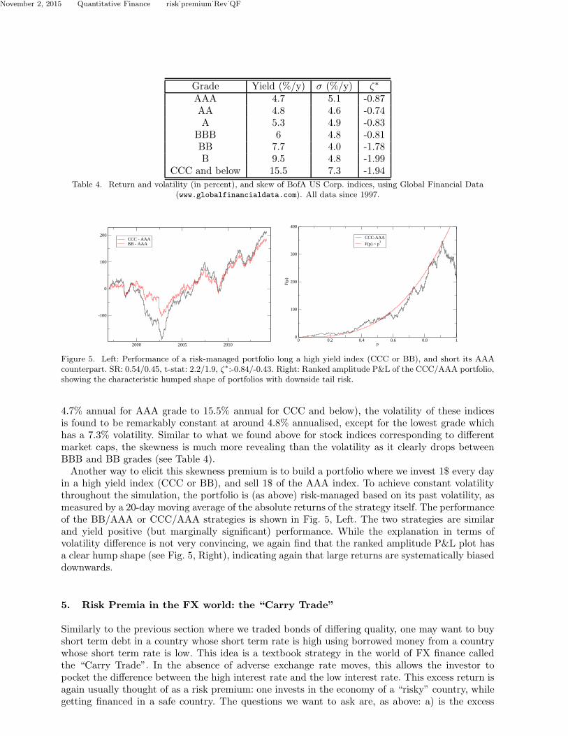
In the world of fixed income, credit risk is gauged by the investment grade of the correspondingbond, and one should in principle expect higher yields for lower investment grades (i.e. riskierbonds). We have studied corporate bond portfolios, using Global Financial Data time series forUS bond total return data.1 We have used the BofA Corp. total return index suite, that providesdaily bond returns since 1997 for grades going from AAA (safe) to CCC and below (risky). Wehave summarised the average yield, volatility and skewness for each of these indices in Table 4.The first striking observation is that although we cover a variety of grades and yields (ranging from

1In this paper, we only study US corporate debt, but we believe our results have a more universal scope. For example, we havechecked that a portfolio of international 10Y bonds also exhibits the same features.


Grade Yield (%/y) σ (%/y) ζ∗

AAA 4.7 5.1 -0.87AA 4.8 4.6 -0.74A 5.3 4.9 -0.83

BBB 6 4.8 -0.81BB 7.7 4.0 -1.78B 9.5 4.8 -1.99

CCC and below 15.5 7.3 -1.94

Table 4. Return and volatility (in percent), and skew of BofA US Corp. indices, using Global Financial Data(www.globalfinancialdata.com). All data since 1997.

2000 2005 2010

-100

0

100

200CCC - AAABB - AAA

0 0.2 0.4 0.6 0.8 1p

0

100

200

300

400

F(p)

CCC-AAA

F(p) ~ p3

Figure 5. Left: Performance of a risk-managed portfolio long a high yield index (CCC or BB), and short its AAAcounterpart. SR: 0.54/0.45, t-stat: 2.2/1.9, ζ∗:-0.84/-0.43. Right: Ranked amplitude P&L of the CCC/AAA portfolio,showing the characteristic humped shape of portfolios with downside tail risk.

4.7% annual for AAA grade to 15.5% annual for CCC and below), the volatility of these indicesis found to be remarkably constant at around 4.8% annualised, except for the lowest grade whichhas a 7.3% volatility. Similar to what we found above for stock indices corresponding to differentmarket caps, the skewness is much more revealing than the volatility as it clearly drops betweenBBB and BB grades (see Table 4).Another way to elicit this skewness premium is to build a portfolio where we invest 1$ every day

in a high yield index (CCC or BB), and sell 1$ of the AAA index. To achieve constant volatilitythroughout the simulation, the portfolio is (as above) risk-managed based on its past volatility, asmeasured by a 20-day moving average of the absolute returns of the strategy itself. The performanceof the BB/AAA or CCC/AAA strategies is shown in Fig. 5, Left. The two strategies are similarand yield positive (but marginally significant) performance. While the explanation in terms ofvolatility difference is not very convincing, we again find that the ranked amplitude P&L plot hasa clear hump shape (see Fig. 5, Right), indicating again that large returns are systematically biaseddownwards.

5. Risk Premia in the FX world: the “Carry Trade”

Similarly to the previous section where we traded bonds of differing quality, one may want to buyshort term debt in a country whose short term rate is high using borrowed money from a countrywhose short term rate is low. This idea is a textbook strategy in the world of FX finance calledthe “Carry Trade”. In the absence of adverse exchange rate moves, this allows the investor topocket the difference between the high interest rate and the low interest rate. This excess return isagain usually thought of as a risk premium: one invests in the economy of a “risky” country, whilegetting financed in a safe country. The questions we want to ask are, as above: a) is the excess


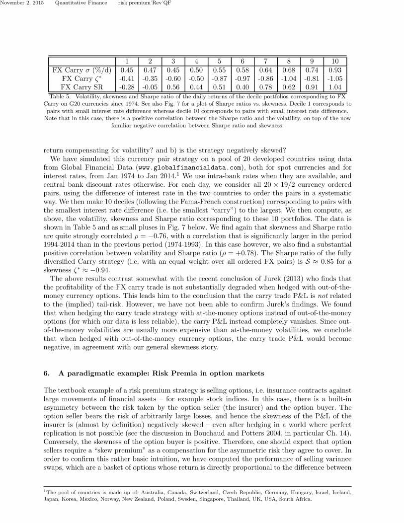
1 2 3 4 5 6 7 8 9 10FX Carry σ (%/d) 0.45 0.47 0.45 0.50 0.55 0.58 0.64 0.68 0.74 0.93

FX Carry ζ∗ -0.41 -0.35 -0.60 -0.50 -0.87 -0.97 -0.86 -1.04 -0.81 -1.05FX Carry SR -0.28 -0.05 0.56 0.44 0.51 0.40 0.78 0.62 0.91 1.04

Table 5. Volatility, skewness and Sharpe ratio of the daily returns of the decile portfolios corresponding to FXCarry on G20 currencies since 1974. See also Fig. 7 for a plot of Sharpe ratios vs. skewness. Decile 1 corresponds topairs with small interest rate difference whereas decile 10 corresponds to pairs with small interest rate difference.Note that in this case, there is a positive correlation between the Sharpe ratio and the volatility, on top of the now

familiar negative correlation between Sharpe ratio and skewness.

return compensating for volatility? and b) is the strategy negatively skewed?We have simulated this currency pair strategy on a pool of 20 developed countries using data

from Global Financial Data (www.globalfinancialdata.com), both for spot currencies and forinterest rates, from Jan 1974 to Jan 2014.1 We use intra-bank rates when they are available, andcentral bank discount rates otherwise. For each day, we consider all 20 × 19/2 currency orderedpairs, using the difference of interest rate in the two countries to order the pairs in a systematicway. We then make 10 deciles (following the Fama-French construction) corresponding to pairs withthe smallest interest rate difference (i.e. the smallest “carry”) to the largest. We then compute, asabove, the volatility, skewness and Sharpe ratio corresponding to these 10 portfolios. The data isshown in Table 5 and as small pluses in Fig. 7 below. We find again that skewness and Sharpe ratioare quite strongly correlated ρ = −0.76, with a correlation that is significantly larger in the period1994-2014 than in the previous period (1974-1993). In this case however, we also find a substantialpositive correlation between volatility and Sharpe ratio (ρ = +0.78). The Sharpe ratio of the fullydiversified Carry strategy (i.e. with an equal weight over all ordered FX pairs) is S ≈ 0.85 for askewness ζ∗ ≈ −0.94.The above results contrast somewhat with the recent conclusion of Jurek (2013) who finds that

the profitability of the FX carry trade is not substantially degraded when hedged with out-of-the-money currency options. This leads him to the conclusion that the carry trade P&L is not relatedto the (implied) tail-risk. However, we have not been able to confirm Jurek’s findings. We foundthat when hedging the carry trade strategy with at-the-money options instead of out-of-the-moneyoptions (for which our data is less reliable), the carry P&L instead completely vanishes. Since out-of-the-money volatilities are usually more expensive than at-the-money volatilities, we concludethat when hedged with out-of-the-money currency options, the carry trade P&L would becomenegative, in agreement with our general skewness story.

6. A paradigmatic example: Risk Premia in option markets

The textbook example of a risk premium strategy is selling options, i.e. insurance contracts againstlarge movements of financial assets – for example stock indices. In this case, there is a built-inasymmetry between the risk taken by the option seller (the insurer) and the option buyer. Theoption seller bears the risk of arbitrarily large losses, and hence the skewness of the P&L of theinsurer is (almost by definition) negatively skewed – even after hedging in a world where perfectreplication is not possible (see the discussion in Bouchaud and Potters 2004, in particular Ch. 14).Conversely, the skewness of the option buyer is positive. Therefore, one should expect that optionsellers require a “skew premium” as a compensation for the asymmetric risk they agree to cover. Inorder to confirm this rather basic intuition, we have computed the performance of selling varianceswaps, which are a basket of options whose return is directly proportional to the difference between

1The pool of countries is made up of: Australia, Canada, Switzerland, Czech Republic, Germany, Hungary, Israel, Iceland,Japan, Korea, Mexico, Norway, New Zealand, Poland, Sweden, Singapore, Thailand, UK, USA, South Africa.


0 0.2 0.4 0.6 0.8 1p

0

200

400

600

800

1000

F(p)

rankedchronological

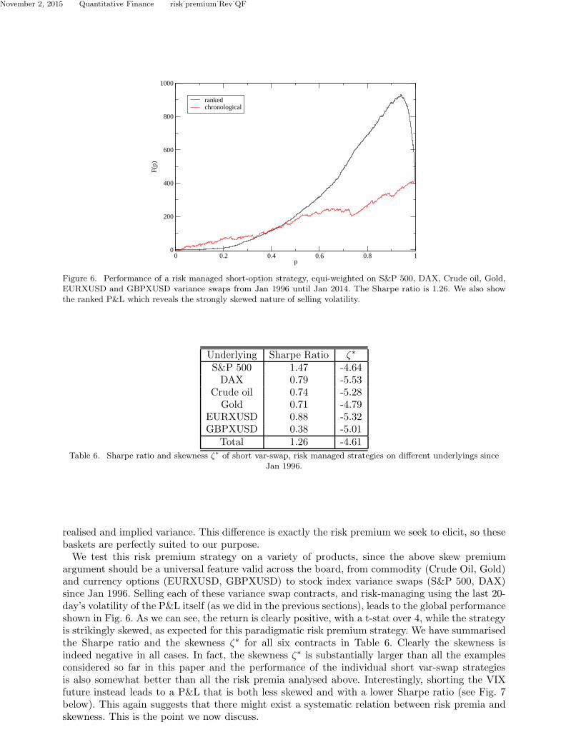
Figure 6. Performance of a risk managed short-option strategy, equi-weighted on S&P 500, DAX, Crude oil, Gold,EURXUSD and GBPXUSD variance swaps from Jan 1996 until Jan 2014. The Sharpe ratio is 1.26. We also showthe ranked P&L which reveals the strongly skewed nature of selling volatility.

Underlying Sharpe Ratio ζ∗

S&P 500 1.47 -4.64DAX 0.79 -5.53

Crude oil 0.74 -5.28Gold 0.71 -4.79

EURXUSD 0.88 -5.32GBPXUSD 0.38 -5.01

Total 1.26 -4.61

Table 6. Sharpe ratio and skewness ζ∗ of short var-swap, risk managed strategies on different underlyings sinceJan 1996.

realised and implied variance. This difference is exactly the risk premium we seek to elicit, so thesebaskets are perfectly suited to our purpose.We test this risk premium strategy on a variety of products, since the above skew premium

argument should be a universal feature valid across the board, from commodity (Crude Oil, Gold)and currency options (EURXUSD, GBPXUSD) to stock index variance swaps (S&P 500, DAX)since Jan 1996. Selling each of these variance swap contracts, and risk-managing using the last 20-day’s volatility of the P&L itself (as we did in the previous sections), leads to the global performanceshown in Fig. 6. As we can see, the return is clearly positive, with a t-stat over 4, while the strategyis strikingly skewed, as expected for this paradigmatic risk premium strategy. We have summarisedthe Sharpe ratio and the skewness ζ∗ for all six contracts in Table 6. Clearly the skewness isindeed negative in all cases. In fact, the skewness ζ∗ is substantially larger than all the examplesconsidered so far in this paper and the performance of the individual short var-swap strategiesis also somewhat better than all the risk premia analysed above. Interestingly, shorting the VIXfuture instead leads to a P&L that is both less skewed and with a lower Sharpe ratio (see Fig. 7below). This again suggests that there might exist a systematic relation between risk premia andskewness. This is the point we now discuss.


Underlying Vol/SR corr. Skewness/SR corrBonds -0.69 -0.36

Intl. IDX -0.45 -0.38SMB -0.42 -0.89UMD -0.63 -0.85

FX Carry +0.78 -0.76HML +0.03 +0.64LoV -0.98 +0.23

TREND +0.23 +0.58

Table 7. Correlation coefficient ρ between volatility and Sharpe ratio, and between skewness and Sharpe ratio forall strategies investigated in this paper, and for a 50-day trend following strategy across various futures markets. Inmost cases, and counter-intuitively, correlation with volatility is found to be negative or zero – note in particularthe Low Vol anomaly (LoV). Correlation with skew, on the other hand, is chiefly negative, showing that the main

determinant of risk premium must be skewness and not volatility. Trend, HML and LoV are clear outliers.

7. Risk premium is Skewness premium

7.1. A remarkable plot

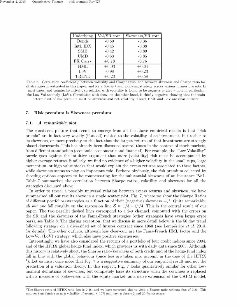
The consistent picture that seems to emerge from all the above empirical results is that “riskpremia” are in fact very weakly (if at all) related to the volatility of an investment, but rather toits skewness, or more precisely to the fact that the largest returns of that investment are stronglybiased downwards. This has already been discussed several times in the context of stock markets,from different standpoints (economic, econometric and financial). For example, the “Low Volatility”puzzle goes against the intuitive argument that more (volatility) risk must be accompanied byhigher average returns. Similarly, we find no evidence of a higher volatility in the small caps, largemomentum, or high value stocks that would explain the excess returns associated to these factors,while skewness seems to play an important role. Perhaps obviously, the risk premium collected byshorting options appears to be compensating for the substantial skewness of an insurance P&L.Table 7 summarises the correlation between Sharpe ratios, volatility and skewness for all thestrategies discussed above.In order to reveal a possibly universal relation between excess returns and skewness, we have

summarised all our results above in a single scatter plot, Fig. 7, where we show the Sharpe Ratiosof different portfolios/strategies as a function of their (negative) skewness −ζ∗. Quite remarkably,all but one fall roughly on the regression line S ≈ 1/3 − ζ∗/4. This is the central result of ourpaper. The two parallel dashed lines correspond to a 2-σ channel, computed with the errors onthe SR and the skewness of the Fama-French strategies (other strategies have even larger errorbars), see Table 8. The glaring exception, that we discuss in more detail below, is the 50 day trendfollowing strategy on a diversified set of futures contract since 1960 (see Lemperiere et al. 2014,for details). The other outliers, although less clear-cut, are the Fama-French HML factor and theLow-Vol (LoV) strategy, which also have positive skewnesses.Interestingly, we have also considered the returns of a portfolio of four credit indices since 2004,

and of the HFRX global hedge fund index, which provides us with daily data since 2003. Althoughthis history is relatively short, the Sharpe ratio/skewness of both credit and of the hedge fund indexfall in line with the global behaviour (once fees are taken into account in the case of the HFRX1). Let us insist once more that Fig. 7 is a suggestive summary of our empirical result and not theprediction of a valuation theory. In this respect, Fig. 7 looks qualitatively similar for other low-moment definitions of skewness, but completely loses its structure when the skewness is replacedwith a measure of coskewness with the equity market, as a naive extension of the CAPM model,

1The Sharpe ratio of HFRX with fees is 0.48, and we have corrected this to yield a Sharpe ratio without fees of 0.85. Thisassumes that funds run at a volatility of around ∼ 10% and have a classic 2 and 20 fee structure.


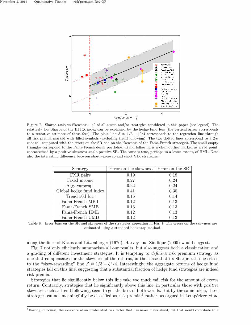
Figure 7. Sharpe ratio vs Skewness −ζ∗ of all assets and/or strategies considered in this paper (see legend). Therelatively low Sharpe of the HFRX index can be explained by the hedge fund fees (the vertical arrow correspondsto a tentative estimate of these fees). The plain line S ≈ 1/3 − ζ∗/4 corresponds to the regression line throughall risk premia marked with filled symbols (excluding trend following). The two dotted lines correspond to a 2-σchannel, computed with the errors on the SR and on the skewness of the Fama-French strategies. The small emptytriangles correspond to the Fama-French decile portfolios. Trend following is a clear outlier marked as a red point,characterised by a positive skewness and a positive SR. The same is true, perhaps to a lesser extent, of HML. Notealso the interesting difference between short var-swap and short VIX strategies.

Strategy Error on the skewness Error on the SR

FXR pairs 0.19 0.18Fixed income 0.27 0.24Agg. varswaps 0.22 0.24

Global hedge fund index 0.41 0.30Trend 50d fut. 0.16 0.14

Fama-French MKT 0.12 0.13Fama-French SMB 0.13 0.13Fama-French HML 0.12 0.13Fama-French UMD 0.12 0.13

Table 8. Error bars on the SR and skewness of the strategies appearing in Fig. 7. The errors on the skewness areestimated using a standard bootstrap method.

along the lines of Kraus and Litzenberger (1976), Harvey and Siddique (2000) would suggest.Fig. 7 not only efficiently summarises all our results, but also suggests both a classification and

a grading of different investment strategies. It is tempting to define a risk premium strategy asone that compensates for the skewness of the returns, in the sense that its Sharpe ratio lies closeto the “skew-rewarding” line S ≈ 1/3 − ζ∗/4. Interestingly, the aggregate returns of hedge fundstrategies fall on this line, suggesting that a substantial fraction of hedge fund strategies are indeedrisk premia.Strategies that lie significantly below this line take too much tail risk for the amount of excess

return. Contrarily, strategies that lie significantly above this line, in particular those with positiveskewness such as trend following, seem to get the best of both worlds. But by the same token, thesestrategies cannot meaningfully be classified as risk premia;1 rather, as argued in Lemperiere et al.

1Barring, of course, the existence of an unidentified risk factor that has never materialised, but that would contribute to a


(2014), these excess returns must represent genuine market anomalies, or “pure α”.

7.2. Three interesting exceptions: HML, LoV & Trend following

Let us dwell a little longer on our outliers: trend following, HML and LoV. The daily skewness ofthese portfolios is significantly positive, respectively ζ∗ = +0.43, ζ∗ = +0.27 and ζ∗ = +0.18, andyet their performance is highly significant and universal across geographical zones.The concept of risk premium applied to HML and to LoV is indeed problematic. Intuitively,

high book-to-price corresponds to “value” stocks that are usually considered safe and defensive,while low book-to-price corresponds to “growth” stocks, i.e. a risky bet on future earnings. Thisis confirmed by the results of Table 3 above, which shows that growth stocks are indeed morenegatively skewed than value stocks, in line with our definition of risk, but indeed making HMLan outlier in Fig 7.1 For LoV, the paradox is even greater: in what sense can it be risky to investon low-volatility stocks and short high-volatility stocks? It seems to us quite reasonable that LoVcannot be understood as a risk premium.Turning now to the nature of trend following, it could in fact have been anticipated that its

skewness should be positive. This is because trend following is profitable, by definition, when thelong term realised volatility is larger than the short term volatility (Fung and Hsieh 1997). Inother words, trend following is akin to a “long gamma” strategy, and is thus expected to have anoppositely signed skewness to that of options. Correspondingly, the skewness of monthly returnsis found to be even more positive than that of daily returns (ζ∗month = +1.72). Hence, the highlysignificant excess returns of trend following strategies in the last two centuries (see Lemperiere et al.2014, for a recent discussion) seem difficult to ascribe to any reasonably defined risk premium. Theprofitability of trend following appears to be a genuine market anomaly, plausibly of behaviouralorigin.2 We find our plot Fig. 7 interesting in the sense that trend following and (albeit to a lesserextent) HML and LoV can be clearly identified as outliers.

8. Discussion and Conclusions

8.1. Skewness vs. co-skewness

Our central result, conveyed by Fig. 7 above, is that skewness is indeed the main determinant ofrisk premia, with an approximately linear relation between the Sharpe ratio S of a risk premiumstrategy and its skewness ζ∗.From a formal point of view, this finding can be qualitatively interpreted within the classi-

cal framework of utility theory. Provided the third derivative of the utility function is positive,skewness-comparable P&Ls can be ordered, and negatively skewed strategies should be com-pensated by higher returns to remain attractive, as amply confirmed by lottery experiments(Garrett and Russell 1999, Astebro et al. 2008). However, previous attempts to include formallythe effect of skewness in valuation theories have led to an extended formulation of the CAPM(Kraus and Litzenberger 1976, Harvey and Siddique 2000), where the co-skewness of a given stockwith the market – rather than the skewness itself – should determine the excess return of that stock.The idea here is that idiosyncratic skewness is diversifiable and should not lead to excess returns;

negative skewness if it did.1However, to add to the confusion, the skewness of the monthly returns of the HML strategy, although more noisy, appears tochange sign (ζ∗

month= −0.56). This suggests that more work is necessary to fully understand the nature of the HML factor,

which is actually known to have long periods of draw-downs (like during the Internet bubble) where the effect appears to bemore in line with a standard risk premium interpretation.2The attentive reader might be puzzled by the fact that trend following has a positive skewness, while market neutral momentum(i.e. UMD) has a negative skewness, as shown above. Still, the two strategies should hinge upon the same underlying behaviouralbiases. This paradox will be discussed in a forthcoming publication.


only the exposure to global market shocks should play a role. As shown by Kraus and Litzenberger(1976), Harvey and Siddique (2000), Harvey et al. (2010) (and more recently in Kelly and Hao2013), this idea seems to have clear merits in the context of stock markets.However, this is not the route we have taken in this paper, for several reasons. First, we tend

to be very suspicious about equilibrium arguments leading to CAPM-like specifications. As amplydemonstrated empirically – including in the present study – market anomalies are numerous andstrong, and theoretical predictions based on arbitrage and rational behaviour not very compelling.Second, our results do not concern the behaviour of individual stocks but rather focus on theprofitability of “factors” in a wide sense – from Fama-French factors to bond, FX and volatility carrytrades. Transposing the coskewness idea of Kraus and Litzenberger (1976), Harvey and Siddique(2000) in the present context would first require the definition of a global “risk factor” that drivesall risk premia, much as the market factor drives individual stocks. This is essentially the contentof the proposal of Rietz (1988), Barro (2006), Santa-Clara and Yan (2010): all these risk premiain fact represent exposure to the same “catastrophic” Black-Swan risk, that would – if realised –spread out over many different asset classes. We have tried to test this idea directly by studyingthe correlation matrix of all the risk premia strategies studied above, with the hope of identifying adominant mode in the PCA, that would define a global risk factor. Perhaps surprisingly, we foundthat the top and second largest eigenvalue of this correlation matrix are not clearly separated(at variance with the correlation matrix of single stocks, that lead to a clear separation betweenthe market and other sub-dominant factors). Furthermore, the structure of the top eigenvector isnot stable in time, which means that it cannot be used as a benchmark to define a meaningfulco-skewness. When (arbitrarily) defining the SPX as the global risk factor, the risk premia co-skewnesses defined a la Kraus and Litzenberger (1976), Harvey and Siddique (2000) were foundto be uncorrelated with the corresponding Sharpe ratio, i.e. all the structure suggested in Fig.7 disappeared. When testing the co-skewness idea restricted to international equity markets, wefound (see Table 1 above) that the Sharpe ratio of the ERP is actually positively (rather thannegatively) correlated with the co-skewness with the US market.

8.2. Skewness, premia & crowded trades

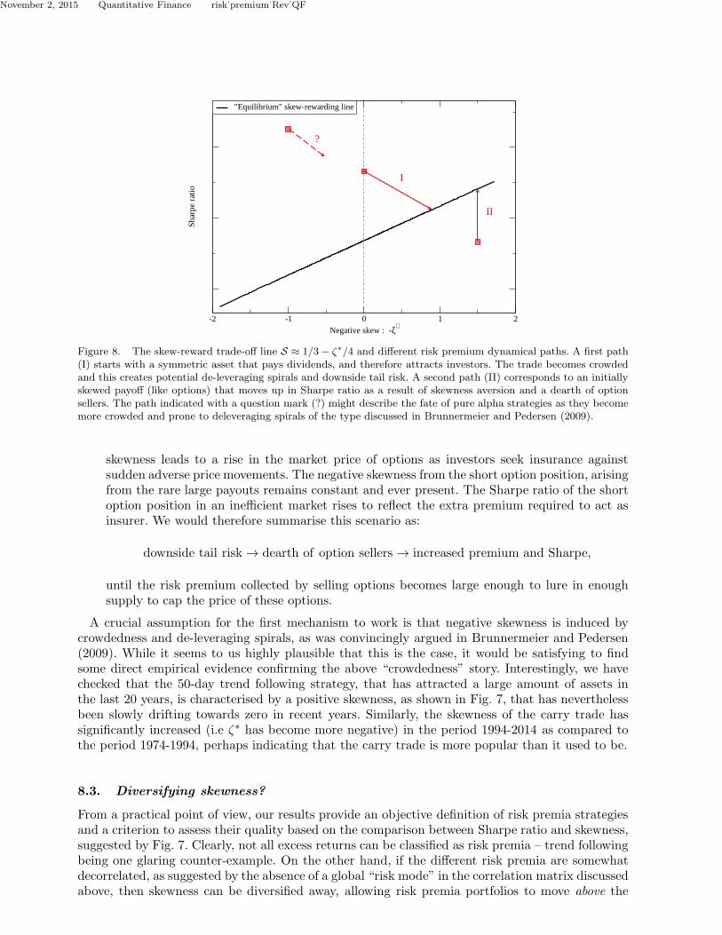
Instead of trying to develop a formal equilibrium argument to explain our findings, we now proposea hand-waving intuitive picture of the mechanism enforcing the trade-off between skewness andexcess returns. Our view is that there may in fact be two fundamentally different ways in whichrisk premia reach the skew-reward trade-off line in Fig. 7:

• In many situations, one buys an asset because of an expected stream of payments, like div-idends for stocks, coupons for bonds, interest rate differences for currency pairs, etc. Thisintrinsic source of returns attracts a crowd of investors that generate a price increase butsimultaneously create the risk of a crash, induced by a self-fulfilling panic or “bank run”mechanism, due to the crowdedness of the trade. Schematically:

dividends → buyers → crowdedness → price increase and downside tail risk.

As illustrated in Fig. 8, crowdedness decreases returns and increases downside tail risk. Botheffects limit the number of additional investors and stabilise the market around an acceptableskewness/excess return trade-off.

• In other situations, downside tail risks pre-exist and it is their very existence that leads toexcess returns. A perfect example is provided by option markets. Since options are insurancecontracts, their payoff profile is by construction skewed - negatively for option sellers andpositively for option buyers. In an efficient market, the fair price of options is such that theiraverage payoff is zero, no risk premium exists and the Sharpe ratio of being long or shortoptions is zero. However, the presence of fat tails and a natural investor preference for positive


-2 -1 0 1 2Negative skew : -ζ∗

0

0.5

1

Shar

pe r

atio

"Equilibrium" skew-rewarding line

?

I

II

Figure 8. The skew-reward trade-off line S ≈ 1/3− ζ∗/4 and different risk premium dynamical paths. A first path(I) starts with a symmetric asset that pays dividends, and therefore attracts investors. The trade becomes crowdedand this creates potential de-leveraging spirals and downside tail risk. A second path (II) corresponds to an initiallyskewed payoff (like options) that moves up in Sharpe ratio as a result of skewness aversion and a dearth of optionsellers. The path indicated with a question mark (?) might describe the fate of pure alpha strategies as they becomemore crowded and prone to deleveraging spirals of the type discussed in Brunnermeier and Pedersen (2009).

skewness leads to a rise in the market price of options as investors seek insurance againstsudden adverse price movements. The negative skewness from the short option position, arisingfrom the rare large payouts remains constant and ever present. The Sharpe ratio of the shortoption position in an inefficient market rises to reflect the extra premium required to act asinsurer. We would therefore summarise this scenario as:

downside tail risk → dearth of option sellers → increased premium and Sharpe,

until the risk premium collected by selling options becomes large enough to lure in enoughsupply to cap the price of these options.

A crucial assumption for the first mechanism to work is that negative skewness is induced bycrowdedness and de-leveraging spirals, as was convincingly argued in Brunnermeier and Pedersen(2009). While it seems to us highly plausible that this is the case, it would be satisfying to findsome direct empirical evidence confirming the above “crowdedness” story. Interestingly, we havechecked that the 50-day trend following strategy, that has attracted a large amount of assets inthe last 20 years, is characterised by a positive skewness, as shown in Fig. 7, that has neverthelessbeen slowly drifting towards zero in recent years. Similarly, the skewness of the carry trade hassignificantly increased (i.e ζ∗ has become more negative) in the period 1994-2014 as compared tothe period 1974-1994, perhaps indicating that the carry trade is more popular than it used to be.

8.3. Diversifying skewness?

From a practical point of view, our results provide an objective definition of risk premia strategiesand a criterion to assess their quality based on the comparison between Sharpe ratio and skewness,suggested by Fig. 7. Clearly, not all excess returns can be classified as risk premia – trend followingbeing one glaring counter-example. On the other hand, if the different risk premia are somewhatdecorrelated, as suggested by the absence of a global “risk mode” in the correlation matrix discussedabove, then skewness can be diversified away, allowing risk premia portfolios to move above the


regression line shown in Fig. 7. That this may indeed be possible is illustrated by the orange “star”shown in Fig. 7, corresponding to a synthetic Diversified Risk Premia portfolio, with an equalweight on Long stock indices, Short Vol, FX Carry and CDS indices. We believe that this is whatgood “alternative beta” managers should strive to achieve.

Appendix: Ranked Amplitude P&Ls and an alternative definition of Skewness

Let us consider a random variable r (the returns) with a certain probability density P (r). Weassume that r has been standardised (i.e. r has zero mean and unit variance). We will denote asx = |r| ≥ 0 the amplitude of r. From the definition of the ranked P&L function F0(p), one has:

F0(p) =

∫ x(p)

0dy y [P (y)− P (−y)] , (3)

where x(p) is the p-quantile of |r|, defined as p =∫ x(p)0 dr(P (r) + P (−r)). We will introduce the

symmetric and antisymmetric contributions to P as:

Ps(r) = P (r) + P (−r), Pa(r) = P (r)− P (−r). (4)

Note that for generic distributions, P (r) ≈r→0 P (0) − P ′(0)r + ..., leading to lowest order (whenp → 0) to x(p) ≈ p/2P (0) and therefore

F0(p) ∼ −P ′(0)/12 × (p/P (0))3, (5)

i.e. a generic ∝ p3 behaviour for small p.Now, our definition of skewness is:

ζ∗ := −100

∫ 1

0dpF0(p) = −100

∫

∞

0dxPs(x)

∫ x

0dy yPa(y). (6)

It is interesting to give an alternative, intuitive interpretation of this definition. After simple ma-nipulations, one finds:

F0(p) = E[|r||r < −x(p)]− E[|r||r > −x(p)]. (7)

F0(p) therefore compares the average amplitude of large negative and large positive returns. ζ∗ isan average of this difference over all possible quantile choices. It might also be useful to relate ζ∗

to the standard definition of skewness ζ3 (defined through the third cumulant of a distribution) inthe limit of weakly non-Gaussian distributions:

P (r) =

[

1− ζ33!

d3

dr3+

κ

4!

d4

dr4+ ...

]

1√2π

e−r2/2, (8)

where κ is the kurtosis; finally leading to

ζ∗ =25

6πζ3 (1−

κ

24+ ...) ≈ 1.273 ζ3 (1−

κ

24+ ...) (9)

Note that ζ∗ does not require the existence of the third moment of the distribution, and remainswell defined for all distributions with a finite first moment. In fact, an even weaker condition issufficient: the distribution should fall out faster than |r|−3/2.


3 4 5 6 7 8ν+ (with fixed ν− = 3.5)

-5

-4

-3

-2

-1

0

1

2

3

skew

ness

Standard definition (third moment)New definition (ranked amplitude)

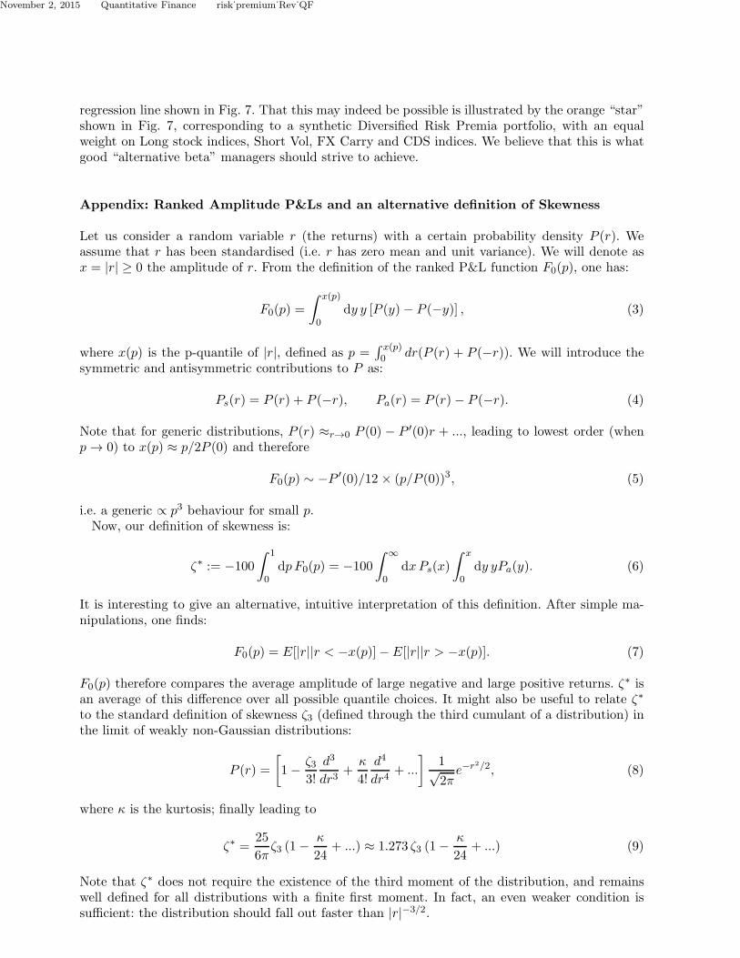
Figure 9. ζ3 and ζ∗ as a function of ν+ for a fixed value of ν− = 3.5, for the assymetric Student-t distribution definedin the text.

It is interesting to compare ζ∗ to the classical definition of skewness ζ3 is a concrete case. Wechoose an assymetric Student-t distribution, defined as (Jones and Faddy 2003):

P (r) = N

1 +r

√

ν++ν−

2 + r2

ν−+1

2

1− r√

ν++ν−

2 + r2

ν++1

2

(10)

which behaves asymptotically as:

P (r) ∼r→±∞ const.|r|−1−ν± . (11)

The classical skewness ζ3 is finite only when ν± > 3, whereas ζ∗ remains finite as long as ν± > 1/2.While the latter condition is always satisfied by financial data, many authors have reported thatν± is actually close to 3 for most markets. As a numerical exercice, we compute both ζ3 and ζ∗

as a function of ν+ > 3, for a fixed value of ν− = 3.5. The results are shown in Fig. 9. Clearly,the skewness of the distribution is positive when ν+ < ν− and negative otherwise. What we see isthat, as expected from the above general formula, ζ∗ and ζ3 behave similarly when they are bothsmall. However, as ν+ decreases towards 3, ζ3 diverges whereas ζ∗ remains well behaved. In theopposite direction, we see that ζ3 quickly saturates as ν+ increases, while ζ∗ continues to decrease.Therefore, ζ∗ is a better discriminant of the assymetry of the distribution.Finally, let us assume that F0(p) is a humped function of p with a single maximum, corresponding

to a negatively skewed distribution. This means that necessarily Pa(y > 0) is negative for largeenough y > y∗ and positive for smaller ys, and vice-versa for y < 0. Now the cumulative functionof P compared to its symmetrised version is precisely the cumulative of Pa(y):

G(y) =

∫ y

−∞

dr[P (r)− Ps(r)] =

∫ y

−∞

drPa(r) (12)

Since Pa(r) vanishes three times and is positive for large negative r, it is clear that G(y) hastwo symmetric maxima located at ±y∗ and a minimum for y = 0. Now using 0 = F0(p = 1) <y∗

∫

∞

0 drPa(r) and G(0) = −∫

∞

0 drPa(r), one immediately finds that G(0) < 0 for non degeneratedistributions. This proves that G(y) crosses zero twice and only twice, and therefore that P (r) and


Ps(r) are skewness-comparable in the sense of Oja (1981) whenever F0(p) has a unique maximum(or minimum).

References

A. Ang, R. J. Hodrick, Y. Xing, and X. Zhang, The Cross- Section of Volatility and Expected Returns,Journal of Finance, 61, 259-299 (2006).

A. Ang, R. J. Hodrick, Y. Xing, and X. Zhang, High Idiosyncratic Volatility and Low Returns: Internationaland Further US Evidence, Journal of Financial Economics, 91, 1-23 (2009).

T. Astebro, J. Mata, L. Santos-Pinto, Preference for skew in gambling, lotteries and entrepreneurship, work-ing paper (2008).

G. Athayde, R. Flores, Finding a Maximum Skewness Portfolio: A General Solution to Three-MomentsPortfolio Choice, Journal of Economic Dynamics & Control, 28, 1335-1352 (2004).

M. Baker, B. Bradley, J. Wurgler, Benchmarks as limits to arbitrage: understanding the low volatilityanomaly, Financial Analysts Journal 67, 40-54 (2011).

R. J. Barro, Rare Disasters and Asset Markets in the Twentieth Century, Quarterly Journal of Economics121, 823-866 (2006).

D. C. Blitz, P. van Vliet, The Volatility Effect: Lower Risk without Lower Return, Journal of PortfolioManagement, pp. 102-113 (2007).

T. Bollerslev, V. Todorov, Tails, fears, and risk premia. The Journal of Finance 66, 2165-2211 (2011).J.-Ph. Bouchaud, M. Potters, Theory of Financial Risks and Derivative Pricing, 2nd Edition, Cambridge

University Press (2004).M. K. Brunnermeier, L. H. Pedersen, Market Liquidity and Funding Liquidity Rev. Financ. Stud. 22, 2201-

2238 (2009).W. H. Chiu, Skewness preference, risk taking and expected utility maximization, The Geneva Risk and

Insurance Review 2010, 1-22.S. Ciliberti, Y. Lemperiere, A. Beveratos, G. Simon, L. Laloux, M. Potters and J.-Ph. Bouchaud Decon-

structing the Low-Vol anomaly, http://ssrn.com/abstract=2670076, and refs. therein.K. Daniel, T. J. Moskowitz,Momentum Crashes Swiss Finance Institute Research Paper Series 13-61 (2013).A. Damodaran, Equity Risk Premiums (ERP): Determinants, Estimation and Implications, working paper,

2012.P. Fernandez, J. Aguirreamalloa, L. C. Avendano, Market Risk Premium Used in 82 Countries in 2012: A

Survey with 7,192 Answers, IESE Business School Working Paper No. WP-1059-E. Available at SSRN:http://ssrn.com/abstract=2084213

J.-P. Fouque, G. Papanicolaou, R. Sircar, K. Sølna, Multiscale Stochastic Volatility for Equity, Interest Rate,and Credit Derivatives, Cambridge University Press, 2011.

A. Frazzini, L. H. Pedersen, Betting against beta, Journal of Financial Economics 111, 1-25 (2014).W. Fung, D. Hsieh, Survivorship Bias and Investment Style in the Returns of CTAs, Journal of Portfolio

Management, 23, 30-41 (1997).T. Garrett, S. Russell, Gamblers Favor Skewness not Risk: Further Evidence from United States Lottery

Games, Economics Letters, 63, 85-90 (1999).C. Harvey, A. Siddique, Conditional skewness in asset pricing tests, Journal of Finance 55, 1263-1295 (2000).C. R. Harvey, J. C. Liechty, M. W. Liechty, P. Muller, Portfolio selection with higher moments, Quantitative

Finance 10, 469-485 (2010).M. C. Jones, M. J. Faddy (2003), A skew extension of the t distribution, with applications, J. Roy. Statist.

Soc., Ser. B 65, 159174 (2003).J. W. Jurek, Crash-Neutral Currency Carry Trades, ssrn-id1262934, August 2013.D. Kahneman, A. Tversky, Prospect theory: An analysis of decision under risk, Econometrica 47, 263-291

(1979).B. T. Kelly, H. Jiang, Tail Risk and Asset Prices, Chicago Booth Research Paper No. 13-67. Available at

SSRN: http://ssrn.com/abstract=2321243 (2013).R. Kozhan, A. Neuberger, P. Schneider, The Skew Risk Premium in the Equity Index Market, working paper

(2013).A. Kraus and R. H. Litzenberger, Skewness Preference and the Valuation of Risk Assets The Journal of

Finance, 31, 1085-1100 (1976)

http://ssrn.com/abstract=2670076


http://arxiv.org/abs/ssrn-id/1262934



Y. Lemperiere, C. Deremble, P. Seager, M. Potters and J.-Ph. Bouchaud Two centuries of trend followingJournal of Investment Strategies, 3, 41-61 (2014), and refs. therein.

R. Mehra, E. C. Prescott, The Equity Premium: A Puzzle, Journal of Monetary Economics 15, 145-161(1985).

R. Mehra, E. C. Prescott, The Equity Premium in Retrospect, in G. Constantinedes, M. Harris, and R. M.Stulz (Eds.), Handbook of the Economics of Finance (Amsterdam: Elsevier, 2003).

H. Oja, On Location, Scale, Skewness and Kurtosis of Univariate Distributions, Scandinavian Journal ofStatistics, 8, 154-168 (1981).

T. A. Rietz, The Equity Premium Puzzle: A Solution?, Journal of Monetary Economics 22, 117-131 (1988).P. Santa-Clara, S. Yan, Crashes, volatility, and the equity premium: Lessons from S&P 500 options, The

Review of Economics and Statistics 92, 435-451 (2010).W. F. Sharpe, Capital asset prices: A theory of market equilibrium under conditions of risk, Journal of

Finance, 19, 425-442 (1964)M. R.C. van Oordt, C. Zhou, Systematic tail risk, working paper (2013).

Documents

RiskPremia: AsymmetricTail Risks andExcessReturns arXiv ... · theoretical prices, as it allows one to introduce an extra ﬁtting parameter conveniently called the ... (CARA) utility