Master’s Thesis

Road Scene Image Translation from

Day to Night using Semantic

Segmentation

Seung Youp Baek

Department of Computer Science and Engineering

The Graduate School

Sungkyunkwan University

Master’s Thesis

Road Scene Image Translation from

Day to Night using Semantic

Segmentation

Seung Youp Baek

Department of Computer Science and Engineering

The Graduate School

Sungkyunkwan University

Road Scene Image Translation from

Day to Night using Semantic

Segmentation

Seung Youp Baek

A Master's Thesis Submitted to the Department of Computer

Science and Engineering and the Graduate School of

Sungkyunkwan University in partial fulfillment of the

requirements for the degree of Master of Science in

Engineering

October 2020

Supervised by

Sungkil Lee

Major Advisor

This certifies that the Master's Thesis

of Seung Youp Baek is approved.

Committee Chairman :

Committee Member :

Major Advisor :

The Graduate School

Sungkyunkwan University

December 2020

i

Table of Contents

List of Tables ·········· iii

List of Figures ·········· iii

List of Equations ·········· iv

Abstract ·········· v

1. Introduction ·········· 1

2. Related Work ·········· 4

3. Framework ·········· 7

3.1 Brightness Adjustment ·········· 8

3.2 Coarse Depth Estimation ·········· 13

A. Lane Marking Segmentation ·········· 13

B. Edge Detection ·········· 15

C. Line Detection ·········· 17

D. Vanishing Point Detection ·········· 18

E. Coarse Depth Generation ·········· 19

3.3 Light Map Generation ·········· 20

A. Bloom Effect ·········· 21

B. Random Light Splatting ·········· 22

3.4 Composition ·········· 23

3.5 Sensor Noise ·········· 25

A. Random Noise ·········· 25

B. Fixed Patter Noise ·········· 28

C. Color Filter Array and Demosaicing ·········· 29

ii

D. GPU-based Pseudo Random Noise Generation ·········· 31

4. Results ·········· 35

5. Conclusion ·········· 44

6. Limitation and Future Work ·········· 45

References ·········· 47

Korean Abstract ·········· 53

iii

List of Tables

Table 1. ························· 10

Table 2. ························· 33

Table 3. ························· 34

Table 4. ························· 41

Table 5. ························· 43

Table 6. ························· 43

List of Figures

Figure 1. ························· 4

Figure 2. ························· 5

Figure 3. ························· 7

Figure 4. ························· 12

Figure 5. ························· 14

Figure 6. ························· 16

Figure 7. ························· 17

Figure 8. ························· 18

Figure 9. ························· 19

Figure 10. ························· 23

Figure 11. ························· 24

Figure 12. ························· 29

Figure 13. ························· 30

iv

Figure 14. ························· 31

Figure 15. ························· 33

Figure 16. ························· 38

Figure 17. ························· 39

Figure 18. ························· 40

Figure 19. ························· 41

Figure 20. ························· 42

List of Equations

Equation 1. ························· 26

Equation 2. ························· 26

Equation 3. ························· 27

Equation 4. ························· 27

Equation 5. ························· 27

Equation 6. ························· 28

Equation 7. ························· 28

Equation 8. ························· 28

v

Abstract

Road Scene Image Translation from Day to Night using

Semantic Segmentation

The day-to-night image translation is a task where the goal is to translate

the day-time domain image to the night-time domain image. Recent studies

proposed learning-based methods to translate the day-time road scene

dataset into the night-time, the improvements are in progress. However, the

learning-based methods in general are often unpredictable, it is difficult to

obtain the desired results. Also, datasets with preferred annotations may

insufficient or unavailable to use. Hence, in this thesis, we propose a semi-

automatic framework for the day-to-night image translation of road scene

images. Unlike the previous approaches, we do not perform learning to

translate the image. Instead, we utilize the semantic annotations from the

semantic segmentation to perceive the given scene. With the help of semantic

annotation, per-element translations and adjustments are performed to

generate a more plausible night-time image. Then, the feature extractions

such as coarse depth estimation and lighting estimation are performed where

semantic annotations are utilized to avoid unintended translations and enhance

the overall robustness. Lastly, the image sensor noises are modeled and

simulated to obtain even more plausible results. As a consequence, the

experimental results of our framework show that we can synthesize more

vi

plausible night-time road scene images not only in higher-resolution but also

avoid random artifacts, in contrast to previous approaches. Moreover, most

part of our framework operates in GPU; the results can be obtained nearly in

real-time, which shows viable extension for a dataset generation.

Keywords: image processing, computational photography, day-to-night,

semantic segmentation, GPU

1

Chapter 1. Introduction

Image-to-image translation is the problem posed in the computer graphics

and the computer vision, where the main task is to generate a new image from

the given image by interpreting and mapping the two distinct domains and

transferring the features one to another.

In the past, methods have been proposed for the tasks such as denoising

[1], colorization of gray image [2], color transfer [3, 4], and image

segmentation [5], where the features were translated from one to another.

Many learning-based methods have been proposed using the Generative

Adversarial Networks(GANs) [6]; demonstrated astonishing results for the

many different tasks in translating the images with substantial progressions.

Isola et al. [7] approached in GAN-based method and demonstrated results in

many different tasks, such as labels-to-street, black-and-white-to-color,

day-to-night, and more. The CycleGAN [8] proposed a method to train the

network without paired image sets, in contrast to the previous approaches,

shown further improvements in different applications. Likewise, many

learning-based methods have been proposed for various tasks [9-12], but

image translation between the day and night time domain has not been tackled

much yet, compared to the other tasks. Recently several GAN-based methods

were proposed to translate the domain between the day and night images,

especially for the road scene datasets, and the improvements are in progress

[13-19].

2

Despite the successful progressions shown by the learning-based methods

for the day-to-night image translation, yet there are limitations. The

learning-based methods, in general, are difficult to obtain the desired output

as it is unpredictable and difficult to modify. Also, the output may include

artifacts on new scenes. Moreover, obtaining datasets for training with

required annotations may difficult; custom datasets are required, which is

costly in general. Furthermore, translating lightings between the two domains

is challenging, artifacts can be easily produced and it is difficult to accurately

estimate the features. Rather than the day-time image, processing a night-

time image tends to be a more difficult task. This is due to the lack of lightings

and illuminations in the night-scene, where the scene is much darker; it is

difficult to perceive the image and acquire the information. For such reasons,

image translation between the day and night is considered one of the difficult

tasks to perform, and often only rely on learning-based methods.

In this thesis, we present a framework that translates the day-time domain

road scene image to the night-time domain image, semi-automatically. Unlike

the previous studies, we do not perform learning to prevent previous issues.

Instead, we design our framework to utilize the semantic annotations from the

semantic segmentation. By using the semantic annotations, the scene can be

perceived; hence we only focus on day-to-night image translation as the

semantic segmentation for night-time images is yet either coarse or too

erroneous, in contrast to the day-time image. By recognizing each scene

element, per-element translation gets feasible; more plausible and adjustable

results can be obtained. Moreover, we operate most of our framework in GPU,

further improvements in performances are made.

3

To perform a day-to-night image translation, following steps are

performed. First, the proposed framework generates the night-time domain

image by adjusting the brightness of the day-time image. As each scene

element is segmented by the semantic annotations, the per-element

translation is feasible; each scene elements are translated individually.

Thereby, adjustable translation can be performed for a more plausible result.

Then, the feature extractions are performed, such as lane marking

segmentation, coarse depth estimation, and light estimation. Here, the

semantic annotations are used, specific scene elements are selected during

the process. Consequently, unintentional translation and feature extractions

are avoided. Moreover, our framework simulates the noises generated by the

image sensor of the digital camera, as the night-time photographs are likely to

be suffered from the sensor noises, in contrast to the day-time images.

Accordingly, our contribution can be summarized as follow: a new semi-

automatic framework that performs the day-to-night image translation of

road scene images without learning for the translation, but utilizes the

semantic annotations to not only avoid previous issues but also to generate a

more plausible night-time image.

4

Chapter 2. Related Work

In this section, we briefly introduce the previous studies that have

proposed learning-based method for day-to-night image translation

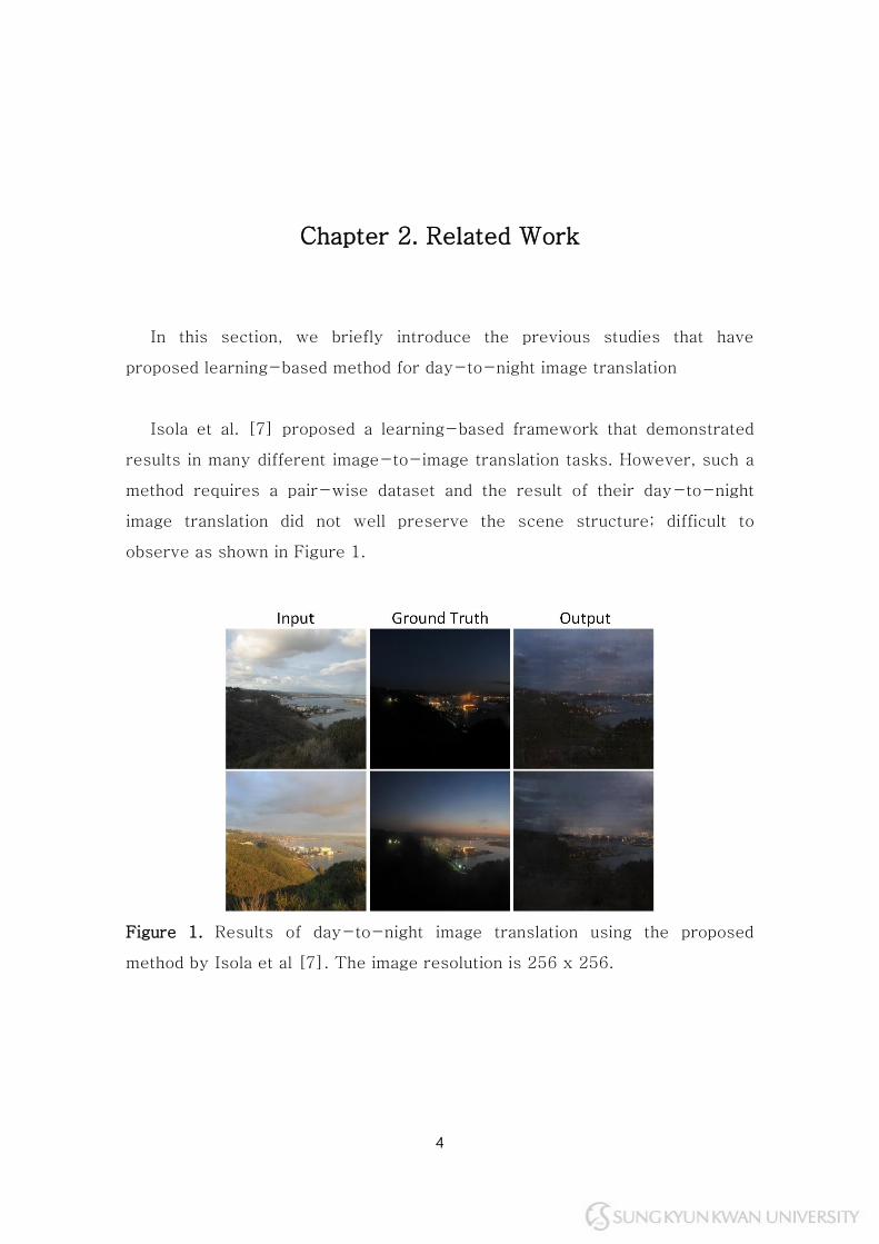
Isola et al. [7] proposed a learning-based framework that demonstrated

results in many different image-to-image translation tasks. However, such a

method requires a pair-wise dataset and the result of their day-to-night

image translation did not well preserve the scene structure; difficult to

observe as shown in Figure 1.

Figure 1. Results of day-to-night image translation using the proposed

method by Isola et al [7]. The image resolution is 256 x 256.

5

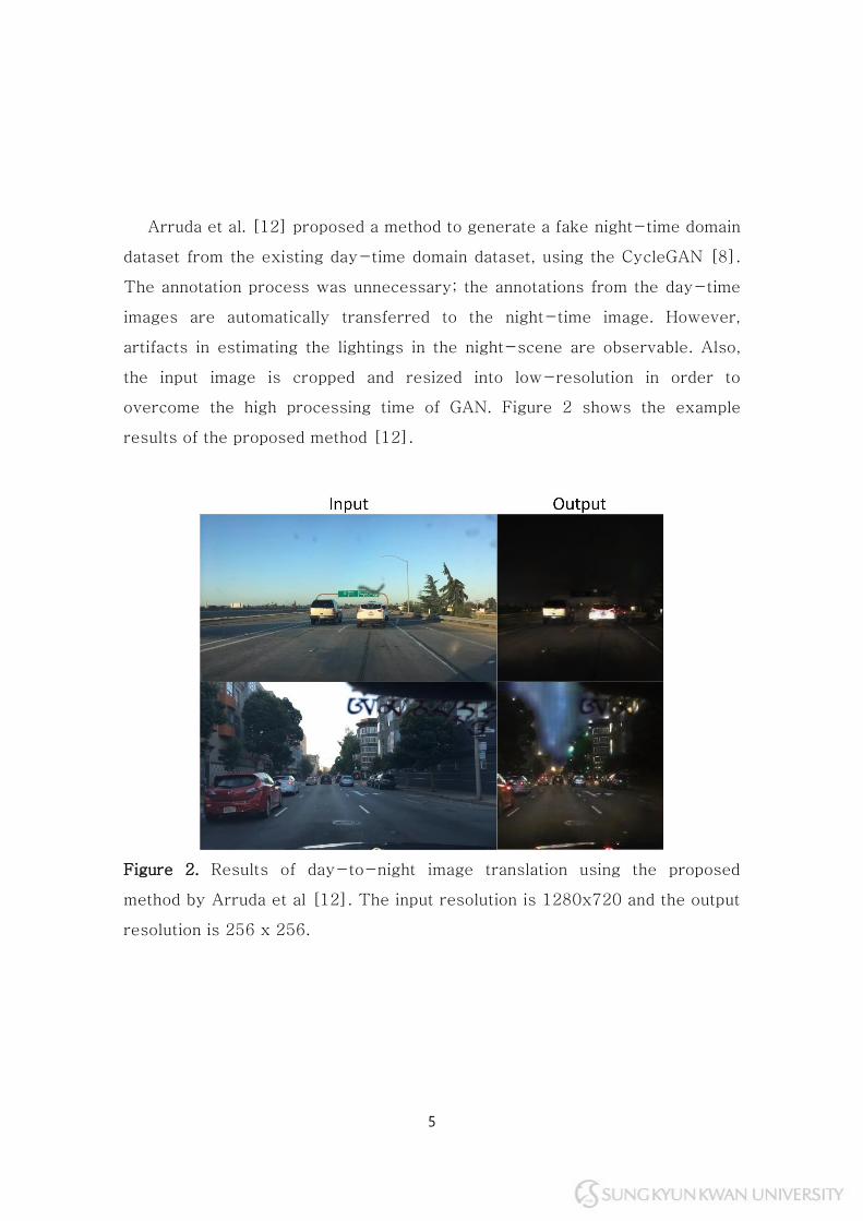
Arruda et al. [12] proposed a method to generate a fake night-time domain

dataset from the existing day-time domain dataset, using the CycleGAN [8].

The annotation process was unnecessary; the annotations from the day-time

images are automatically transferred to the night-time image. However,

artifacts in estimating the lightings in the night-scene are observable. Also,

the input image is cropped and resized into low-resolution in order to

overcome the high processing time of GAN. Figure 2 shows the example

results of the proposed method [12].

Figure 2. Results of day-to-night image translation using the proposed

method by Arruda et al [12]. The input resolution is 1280x720 and the output

resolution is 256 x 256.

6

More recent studies attempt to preserve the structures in the image to

prevent false translation. Huang et al. [14] proposed a method for the day-

to-night image translation while being aware of structures in the image. By

the supervision of the segmentation subtask, the encoder network is trained to

extract image structure information. In contrast to previous studies, the

proposed method generates more plausible results due to the structure-aware

translation.

Similarly, Luan et al. [9] proposed a method for the photorealistic image

style transfer using the Convolutional Neural Networks (CNN). With the

photorealism regulation during the optimization and optional guidance using

semantic segmentation, distortion during the image translation is well-

prevented and the results were improved due to the awareness of the content

in the image.

Most recently, Jiang et al. [16] proposed a learning-based method by

considering not only a structure during the translation but also the style of

translation from day to night; achieved a more plausible night-time image than

previous approaches. Although, the images are scaled into a certain size and

yet artifacts are observable in lightings like the previous approaches.

7

Chapter 3. Framework

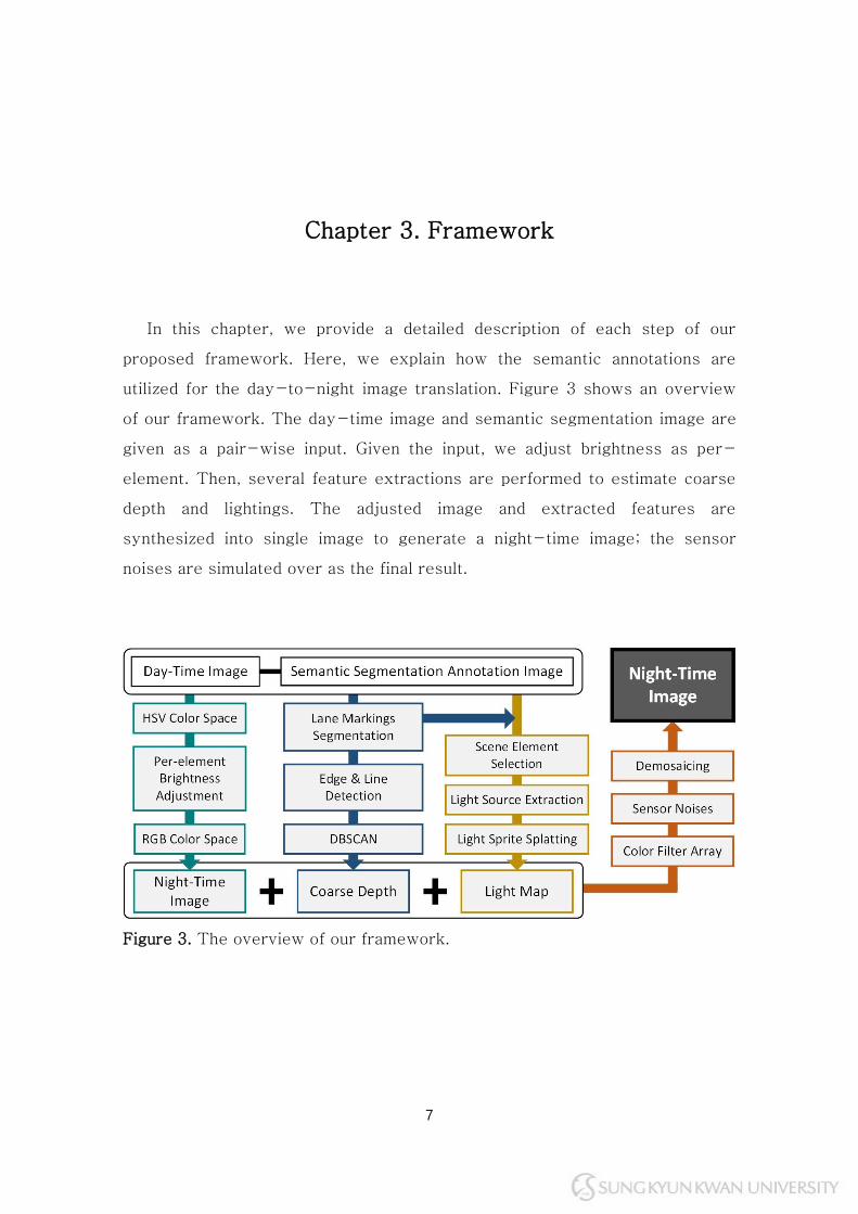
In this chapter, we provide a detailed description of each step of our

proposed framework. Here, we explain how the semantic annotations are

utilized for the day-to-night image translation. Figure 3 shows an overview

of our framework. The day-time image and semantic segmentation image are

given as a pair-wise input. Given the input, we adjust brightness as per-

element. Then, several feature extractions are performed to estimate coarse

depth and lightings. The adjusted image and extracted features are

synthesized into single image to generate a night-time image; the sensor

noises are simulated over as the final result.

Figure 3. The overview of our framework.

8

As our framework utilizes the semantic annotations during the translation,

the semantic annotation image is required along with the day-time image. For

that reason, our framework uses the dataset that provides semantic

segmentation images with annotations. For the experiments, the Cityscapes

[20], KITTI [21], and BDD100K [22] datasets are selected. All 3 datasets

provide pixel-level semantic segmentation images with the corresponding

day-time road scene images. Unlike the other two datasets, BDD100K also

includes the night-time images, but the semantic segmentation images are

partially annotated, which makes difficult to use for night-to-day translation.

Datasets with the provision of semantic segmentation follow certain data

formats for the annotations. Typically, the unique color code is assigned to

each semantic label. Our framework follows the data format used by the

Cityscapes dataset, as the KITTI and BDD100K dataset also follow the same

data format. Thus, the preprocessing for aligning data format is unnecessary.

Figure 4-15 show the example result of each step and features extracted

during the translation. Here, the Cityscape dataset is used for the

demonstration.

1. Brightness Adjustment

One of the major differences between the two domains is the sunlight. Due

to the absence of the sunlight during the night, the night-time image is

significantly darker in contrast to day-time image. Thus, as the first step of

9

our framework, we adjust the brightness of the day-time image to generate

the night-time image.

To adjust the brightness, the image gets converted to HSV color space.

Thereby, only the brightness value (V) of the color for each pixel in the image

can be adjusted. Here, the framework performs the per-element adjustment,

rather than adjusting the brightness of the image globally. This is due to the

difference in the level of exposure between the two domains for each scene

element. For example, the sky is one of the brightest areas in the day-time

image, but it is also the darkest area in the night-time. Hence, the adjustment

is performed locally, each scene element is adjusted individually to obtain a

more plausible night-time image.

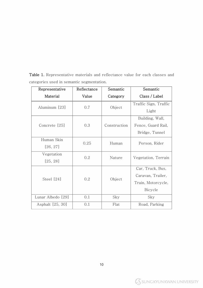
During the adjustment process, the amount of brightness to be reduced for

each scene element is set. Instead of manually setting the value, we used the

reflectance values of different materials. Here, the representative material for

each semantic annotation is assigned; the corresponding reflectance values

are used for the brightness adjustment. Table 1 summarizes the

representative materials and the corresponding reflectance values that we

have assigned for each semantic annotation. The reflectance values are set

between the 0 to 1, which are applied to the brightness value of each image

pixels.

10

Table 1. Representative materials and reflectance value for each classes and

categories used in semantic segmentation.

Representative

Material

Reflectance

Value

Semantic

Category

Semantic

Class / Label

Aluminum [23] 0.7 Object Traffic Sign, Traffic

Light

Concrete [25] 0.3 Construction

Building, Wall,

Fence, Guard Rail,

Bridge, Tunnel

Human Skin

[26, 27] 0.25 Human Person, Rider

Vegetation

[25, 28] 0.2 Nature Vegetation, Terrain

Steel [24] 0.2 Object

Car, Truck, Bus,

Caravan, Trailer,

Train, Motorcycle,

Bicycle

Lunar Albedo [29] 0.1 Sky Sky

Asphalt [25, 30] 0.1 Flat Road, Parking

11

For the ‘human’ category, including the ‘person’ and ‘rider’, the human skin

is selected as the representative material. This is due to the variance in the

appearance of humans, it is nearly impossible to define such appearances as a

single material. Hence, the average reflectance value of different human skin

colors is assigned for both ‘person’ and ‘rider’ label.

For the ‘sky’ label, the lunar albedo is selected as the representative

material. This is due to that the sky cannot be represented as a certain

material that has a surface to measure the reflectance value. Hence, the

amount of radiation that is reflected by the moon is assigned as the

reflectance value.

Unlike any other semantic labels, the ‘unlabeled’ label is assigned to the

pixels where the scene objects are trivial or occluded by other scene objects.

Thus, these group of objects cannot be represented as one, we set the

reflectance value as an average of all other reflectance values.

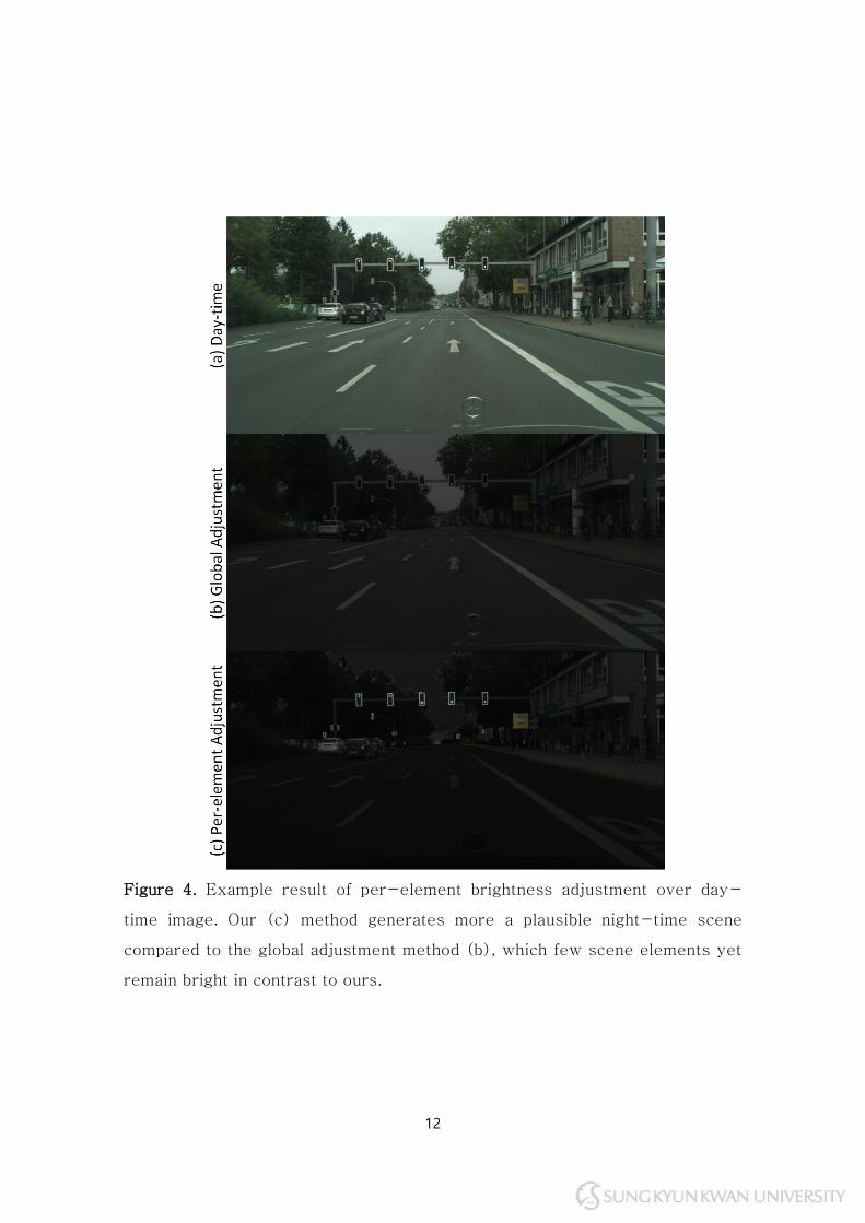
The example result of our brightness adjustments is shown in Figure 4.

The first row shows the day-time image to be adjusted. The second row

shows the result of the night-time image, in which the brightness is adjusted

globally with a 70 percent reduction. The result clearly shows that few scene

elements yet remain bright to be considered as the night. The last row shows

the result of the per-element brightness adjustment, which shows that our

method can generate a more plausible night-time scene.

12

Figure 4. Example result of per-element brightness adjustment over day-

time image. Our (c) method generates more a plausible night-time scene

compared to the global adjustment method (b), which few scene elements yet

remain bright in contrast to ours.

13

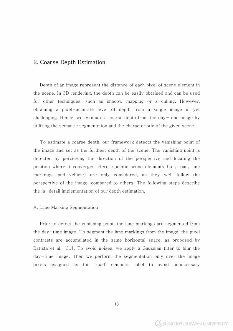
2. Coarse Depth Estimation

Depth of an image represent the distance of each pixel of scene element in

the scene. In 3D rendering, the depth can be easily obtained and can be used

for other techniques, such as shadow mapping or z-culling. However,

obtaining a pixel-accurate level of depth from a single image is yet

challenging. Hence, we estimate a coarse depth from the day-time image by

utilizing the semantic segmentation and the characteristic of the given scene.

To estimate a coarse depth, our framework detects the vanishing point of

the image and set as the furthest depth of the scene. The vanishing point is

detected by perceiving the direction of the perspective and locating the

position where it converges. Here, specific scene elements (i.e., road, lane

markings, and vehicle) are only considered, as they well follow the

perspective of the image, compared to others. The following steps describe

the in-detail implementation of our depth estimation.

A. Lane Marking Segmentation

Prior to detect the vanishing point, the lane markings are segmented from

the day-time image. To segment the lane markings from the image, the pixel

contrasts are accumulated in the same horizontal space, as proposed by

Batista et al. [31]. To avoid noises, we apply a Gaussian filter to blur the

day-time image. Then we perform the segmentation only over the image

pixels assigned as the ‘road’ semantic label to avoid unnecessary

14

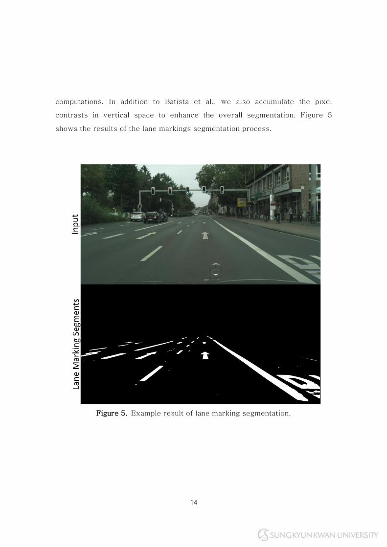
computations. In addition to Batista et al., we also accumulate the pixel

contrasts in vertical space to enhance the overall segmentation. Figure 5

shows the results of the lane markings segmentation process.

Figure 5. Example result of lane marking segmentation.

15

B. Edge Detection

To detect the vanishing point, first the edge detection is performed to

obtain the shape of scene elements. The Canny edge detection [32] is

performed over the semantic segmentation image rather than the day-time

image. This is due to prevent the unnecessary edges being detected and also

to detect edges only from selected scene elements (i.e., road and vehicle) as

our purpose is to obtain the shape of objects and perceive the perspective.

In addition, the edges are also detected from the lane markings in the image.

As the lane markings, in general, are aligned along to the road, this helps to

perceive the scene more precisely and enhance the detection of the vanishing

point.

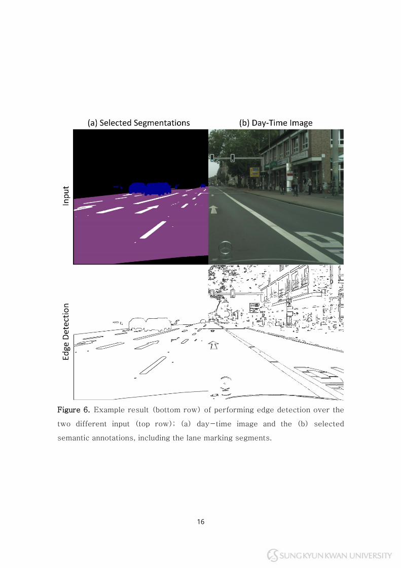
The example result with a comparison between using the semantic

segmentation image and the day-time image is shown in Figure 6. The result

clearly shows that performing the edge detection over semantic segmentation

image with the lane marking segments results in only the shape of scene

elements while the unnecessary edges are all omitted. Such optimization

further enhances the detection of the vanishing point, as the number of edges

to consider is significantly reduced.

16

Figure 6. Example result (bottom row) of performing edge detection over the

two different input (top row); (a) day-time image and the (b) selected

semantic annotations, including the lane marking segments.

17

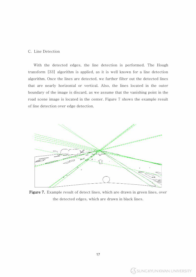
C. Line Detection

With the detected edges, the line detection is performed. The Hough

transform [33] algorithm is applied, as it is well known for a line detection

algorithm. Once the lines are detected, we further filter out the detected lines

that are nearly horizontal or vertical. Also, the lines located in the outer

boundary of the image is discard, as we assume that the vanishing point in the

road scene image is located in the center. Figure 7 shows the example result

of line detection over edge detection.

Figure 7. Example result of detect lines, which are drawn in green lines, over

the detected edges, which are drawn in black lines.

18

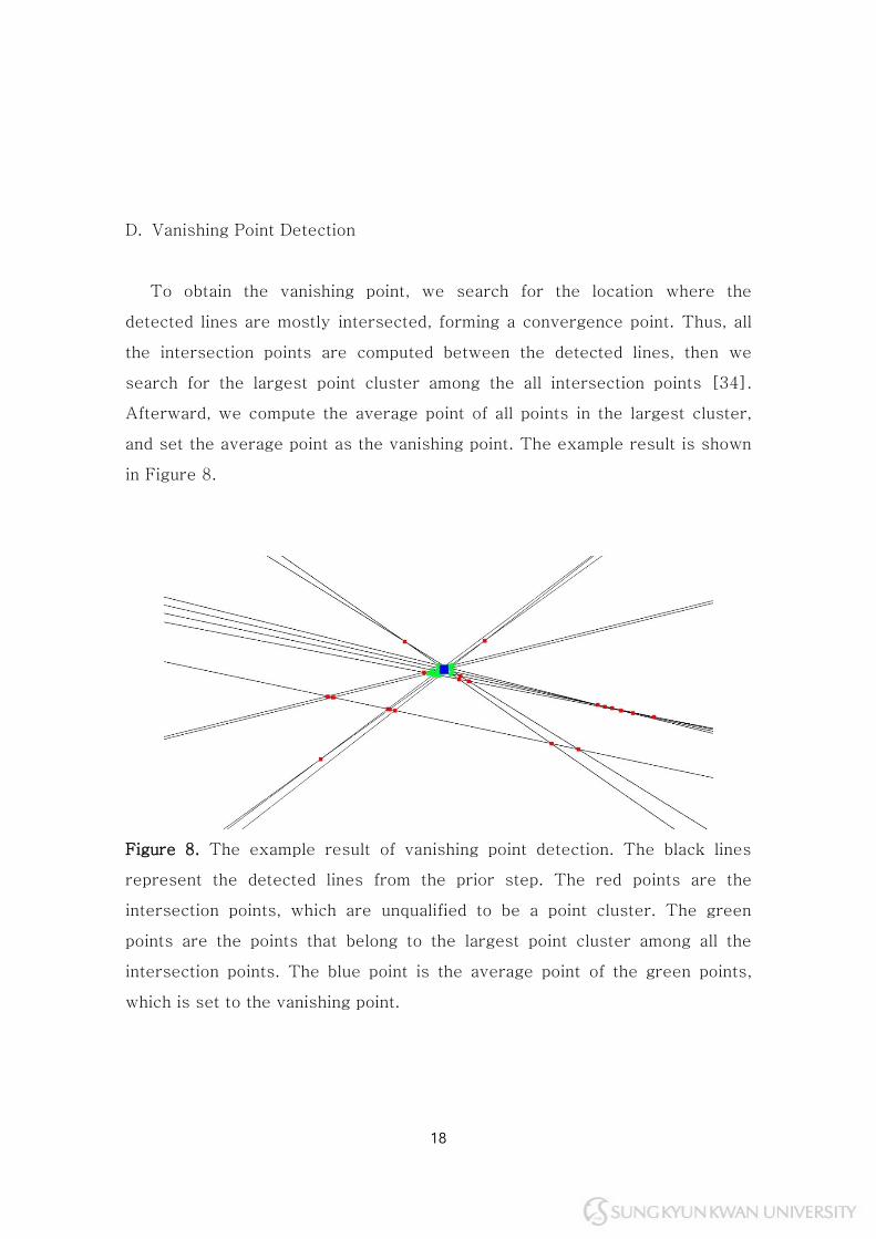
D. Vanishing Point Detection

To obtain the vanishing point, we search for the location where the

detected lines are mostly intersected, forming a convergence point. Thus, all

the intersection points are computed between the detected lines, then we

search for the largest point cluster among the all intersection points [34].

Afterward, we compute the average point of all points in the largest cluster,

and set the average point as the vanishing point. The example result is shown

in Figure 8.

Figure 8. The example result of vanishing point detection. The black lines

represent the detected lines from the prior step. The red points are the

intersection points, which are unqualified to be a point cluster. The green

points are the points that belong to the largest point cluster among all the

intersection points. The blue point is the average point of the green points,

which is set to the vanishing point.

19

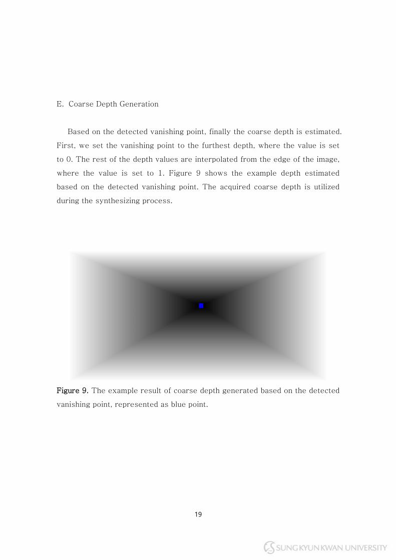
E. Coarse Depth Generation

Based on the detected vanishing point, finally the coarse depth is estimated.

First, we set the vanishing point to the furthest depth, where the value is set

to 0. The rest of the depth values are interpolated from the edge of the image,

where the value is set to 1. Figure 9 shows the example depth estimated

based on the detected vanishing point. The acquired coarse depth is utilized

during the synthesizing process.

Figure 9. The example result of coarse depth generated based on the detected

vanishing point, represented as blue point.

20

3. Light Map Generation

In this section, we describe how the light maps are generated by selecting

specific semantic annotations and segmenting specific pixels from the day-

time image.

Lightings is the other major difference that are easily recognizable between

the two domains, similar to the brightness. Unlike day-time domain, the light

sources during the night-time domain are exceedingly visible due to the

absence of the sunlight. However, estimating the exact presence of the lights

during the night-time domain based on the given day-time domain image is

very challenging, simply due to the uncertainty. Thus, we utilize the semantic

annotations to select specific scene elements to enhance our estimation

process.

First, reflective scene elements (i.e. traffic sign) are selected. The image

pixels belong to the selected elements are automatically added to the separate

light map texture. Here, the segments of lane marking, that we acquired on

previous step, are also added as they are well visible.

Afterward, the pixels that potentially belong to the strong light sources

during the night are extracted. One of the common approaches to segment the

light sources from the image is to compare the pixel values [35, 36]. In

general, the RGB color space is converted to either HSV or CIELAB color

space for better interpretation of the color.

21

Similar to the previous studies, our framework converts the day-time

image into CIELAB color space and extracts light source by extracting certain

color of pixels among selected scene elements (i.e. traffic light and vehicle).

For instance, green, red, and yellow is searched in traffic lights while red and

white is searched for the vehicle. Although such extraction process may be

erroneous in the case of a vehicle, where the exterior color of vehicle may be

same as the light source color, this remains as a challenge [37].

A. Bloom Effect

In the night-time photographs, the strong light source produces artifacts

where the border of lights are extended, shows the glowing effect around.

Such phenomenon is referred to as the diffraction in computer graphics and

photography, often simplified as the ‘bloom effect’ in either rendering or game

engines.

Similarly, our framework applies the bloom effect over the extracted light

sources. In order to know the intensity of the light, which is unknown at the

moment, we generate mipmap of texture which contains the extracted pixels.

Then, the values are sampled from mipmapped texture as the intensity of the

bloom effect, while the Gaussian filter is applied.

22

B. Random Light Splatting

Given the semantic annotations, the light sources from the specific scene

elements (i.e., traffic lights or vehicles) are relatively easy to be estimated, as

their shape, color, and locations are commonly known and expected. In

contrast, lights from other scene elements (i.e., buildings) are almost

impossible to be estimated by either shape, color, or location, as they are

random. The recently proposed learning-based method also produces

significant artifacts in estimating lights in the night-time domain [7, 12], yet it

remains a challenge for a day-to-night image translation to accurately

estimate lightings during the night. Thus, our framework randomly splats pre-

rendered light sprites over the selected scene elements. To avoid light sprites

being rendered over unintended locations (i.e. road or tree), we sample

random position only with the area of selected scene elements (i.e., building).

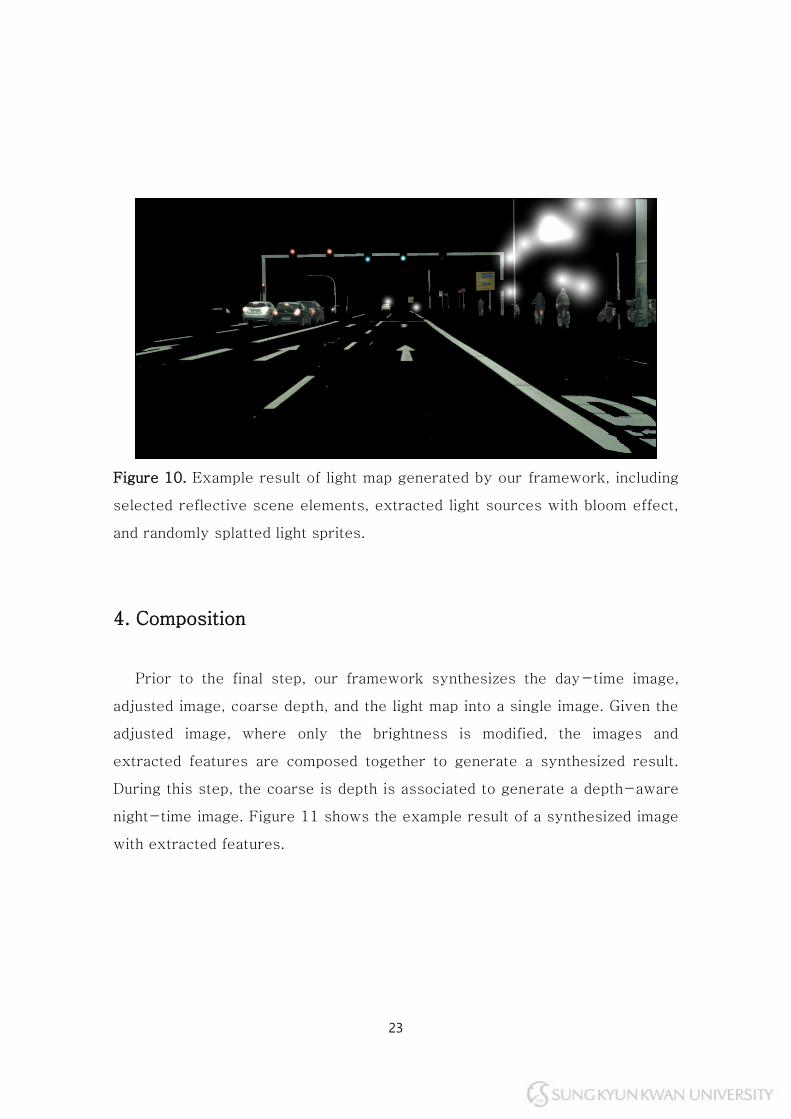
Figure 10 shows the example result of selection of reflective scene

element with estimated light sources by our framework.

23

Figure 10. Example result of light map generated by our framework, including

selected reflective scene elements, extracted light sources with bloom effect,

and randomly splatted light sprites.

4. Composition

Prior to the final step, our framework synthesizes the day-time image,

adjusted image, coarse depth, and the light map into a single image. Given the

adjusted image, where only the brightness is modified, the images and

extracted features are composed together to generate a synthesized result.

During this step, the coarse is depth is associated to generate a depth-aware

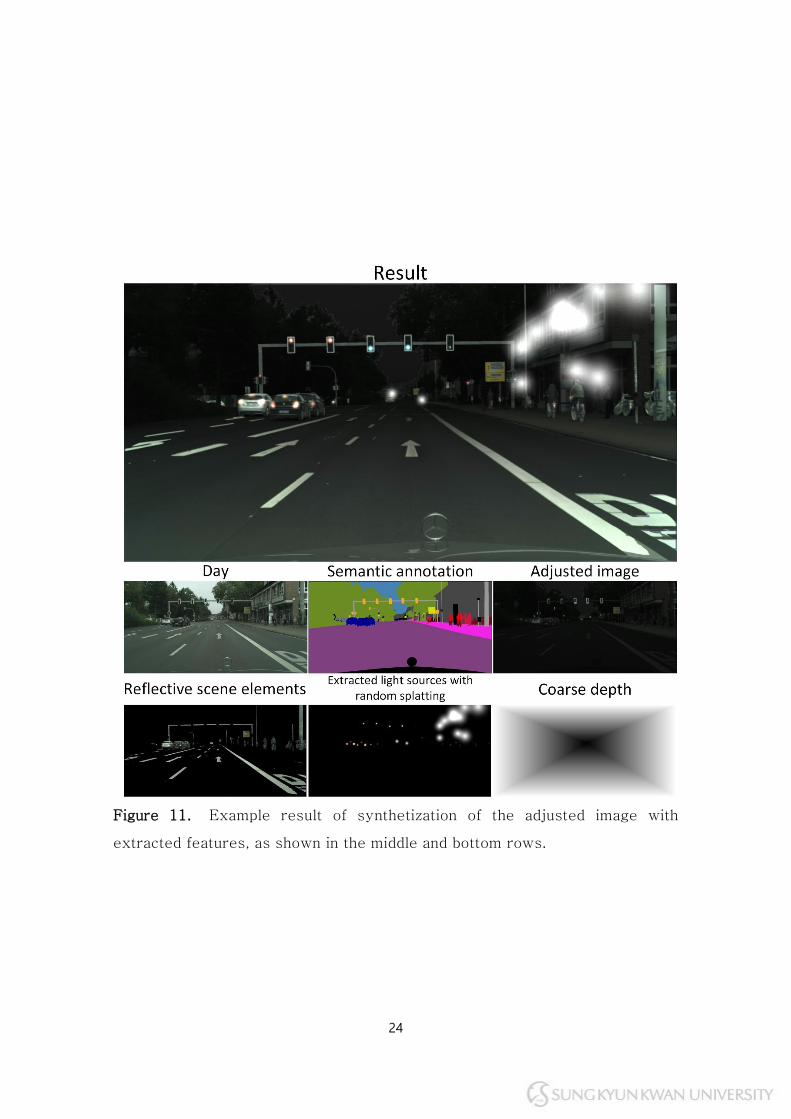
night-time image. Figure 11 shows the example result of a synthesized image

with extracted features.

24

Figure 11. Example result of synthetization of the adjusted image with

extracted features, as shown in the middle and bottom rows.

25

5. Sensor Noise

Photographs taken with the digital cameras suffer from the sensor noises,

due to the characteristic of the image sensor. These noises are mostly

unnoticeable in the day-time images, when the scene is well illuminated. In

contrast, noises are easily noticeable in the night-time images, due to lack of

sunlight. Hence, we model the sensor noises that occur during the digital

camera image processing pipeline to for more plausible result.

In this thesis, we model four different types of sensor noise in the digital

camera image processing pipeline: photon shot noise, dark current shot noise,

photo response non-uniformity (PRNU), and dark signal non-uniformity

(DSNU). The four sensor noises we modeled in our framework can be

categorized into two groups. The photon shot noise and the dark current shot

noise can be grouped as random noise, and the PRNU and DSNU can be

grouped into fixed pattern noise.

A. Random Noise

Random noises refer to the noises that are added to the final image,

affected by the exposure time. Thus, the noise is random for every

photograph taken. The photon shot noise occurs due to the photons randomly

arrives at the image sensor, then captured into the photo-diodes. Thus, each

photo-diodes capture different amount of light. To reduce the noise, shutter

speed can be increased to reduce the gap between the photo-diodes.

26

However, the temperature of the image sensor rises as the exposure time

increases, thermally generated electrons are additionally captured to the

image sensor, which is referred as the dark current shot noise.

The photon shot noise is known to follow the Poisson distribution [38-40],

thus we generate a random number of Poisson distribution for each image

pixel to generate a noise texture. Here, the Poisson mean x𝑝𝑠𝑛 is set as the

Equation 1 [39].

𝑥𝑝𝑠𝑛 = ∫ ∫ ∫ 𝑁(𝜆)𝑄𝐸(𝜆)𝑑𝜆𝑑𝐴𝑑𝑡

𝜆𝑚𝑎𝑥

𝜆𝑚𝑖𝑛

𝐴

𝑇

0

(1)

The T denotes the exposure time, which is the shutter speed of the digital

cameras. A denotes the area of each image pixel in the image sensor. QE

stands for the quantum efficiency of the image sensor, we average the QE for

all visible wavelengths, which is denoted as λ. The N(λ) is the number of

photons arrive at the image sensor per second, and it can be computed as the

Equation 2 [39].

N(λ) =𝐸(𝜆) ∙ 𝜆

ℎ ∙ 𝑐 (2)

The E(λ) is the irradiance of the scene that reaches the image sensor plane,

which can be modeled as Equation 3 [39]. f# denotes the effective focal

length (EFL) and m denotes the magnification, in which the value can be

27

obtained from the specification of a lens. The L denotes the scene irradiance,

which cannot be estimated from a single image and differs for time and space;

a user-defined value is set.

E(λ) = 𝜋𝐿1

1 + 4(𝑓#(1 + |𝑚|))2 (3)

Once the E(λ) is computed, the number of photons reaches the image

sensor plane is computed by multiplying with the Planck-Einstein relation as

shown in Equation 3, where the h is the Planck’s constant and c is the speed

of light. Then, the Poisson mean for photon shot noise is obtained as Equation

1, the noise value for each pixel is computed as Equation 4.

N𝑝𝑠𝑛 = 𝑃𝑜𝑖𝑠(𝑥𝑝) (4)

Similar to the photon shot noise, dark current shot noise is also known to

follow the Poisson distribution [38-40]. Similar to photon shot noise, the

noise can be modeled as Equation 5. The x𝑑𝑠𝑛 denotes the Poisson mean.

N𝑑𝑠𝑛 = 𝑃𝑜𝑖𝑠(𝑥𝑑𝑠𝑛) (5)

Since the dark current shot noise is also affected by the exposure time, the

Poisson mean is computed as the Equation 6. The T denotes the time, similar

to the Equation 1. The d𝑎𝑣𝑔 denotes the average dark currents per second.

28

x𝑑𝑠𝑛 = 𝑇 ∙ 𝑑𝑎𝑣𝑔 (6)

The device-specific parameters used in Equations 1-6 may unavailable to

use. Thus, our framework refers to the device information provided by the

dataset [17, 18] and applies user-defined values as necessary.

B. Fixed Pattern Noise

Fixed pattern noises refer to the noises where the pattern is fixed for the

image sensor. This is due to the imperfection of the image sensor during the

manufacturing process, each photo-diode have variances. The PRNU occurs

by the differences in the responsiveness of each photo-diode in the image

sensor [38-40]. Hence, the number of captured photons will differ for each

photo-diode, even if the same number of photons arrived for all pixels. The

DSNU occurs due to the differences in dark current for each pixel in the image

sensor [38, 39].

Both PRNU and DSNU are known to follow the Gaussian distribution [39,

40], hence we model as Equation 7 and 8 accordingly. The σ𝑝𝑟𝑛𝑢 denotes the

sensitivity of light and σ𝑑𝑠𝑛𝑢 denotes the dark current of each photo-diode in

the image sensor.

N𝑝𝑟𝑛𝑢 = 𝑁(0, 𝜎𝑝𝑟𝑛𝑢2 ) (7)

N𝑑𝑠𝑛𝑢 = 𝑁(0, 𝑇 ∙ 𝜎𝑑𝑠𝑛𝑢2 ) (8)

29

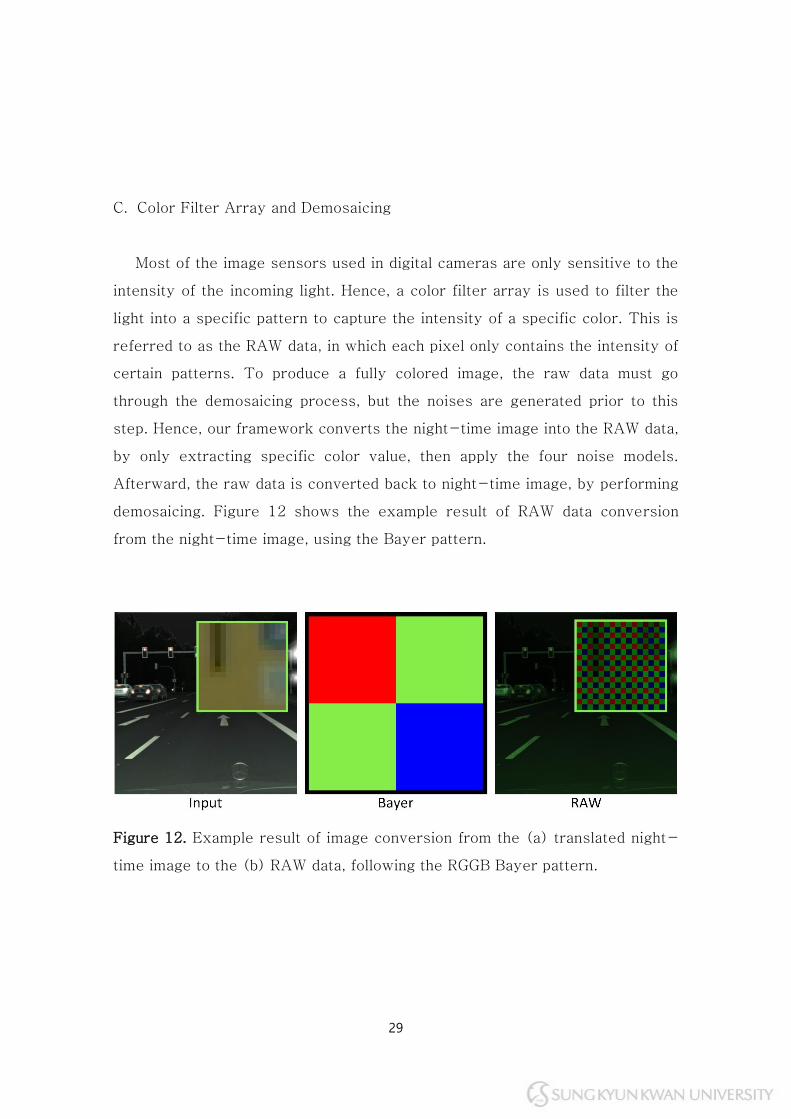
C. Color Filter Array and Demosaicing

Most of the image sensors used in digital cameras are only sensitive to the

intensity of the incoming light. Hence, a color filter array is used to filter the

light into a specific pattern to capture the intensity of a specific color. This is

referred to as the RAW data, in which each pixel only contains the intensity of

certain patterns. To produce a fully colored image, the raw data must go

through the demosaicing process, but the noises are generated prior to this

step. Hence, our framework converts the night-time image into the RAW data,

by only extracting specific color value, then apply the four noise models.

Afterward, the raw data is converted back to night-time image, by performing

demosaicing. Figure 12 shows the example result of RAW data conversion

from the night-time image, using the Bayer pattern.

Figure 12. Example result of image conversion from the (a) translated night-

time image to the (b) RAW data, following the RGGB Bayer pattern.

30

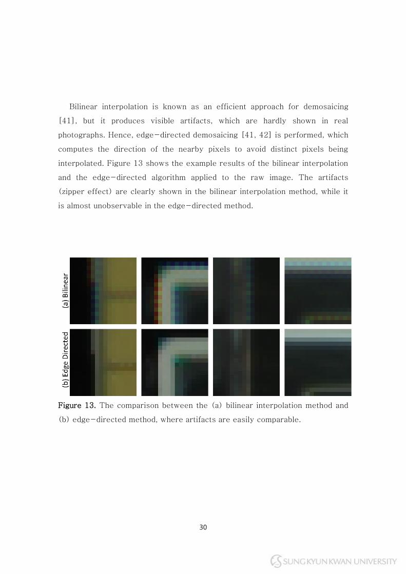
Bilinear interpolation is known as an efficient approach for demosaicing

[41], but it produces visible artifacts, which are hardly shown in real

photographs. Hence, edge-directed demosaicing [41, 42] is performed, which

computes the direction of the nearby pixels to avoid distinct pixels being

interpolated. Figure 13 shows the example results of the bilinear interpolation

and the edge-directed algorithm applied to the raw image. The artifacts

(zipper effect) are clearly shown in the bilinear interpolation method, while it

is almost unobservable in the edge-directed method.

Figure 13. The comparison between the (a) bilinear interpolation method and

(b) edge-directed method, where artifacts are easily comparable.

31

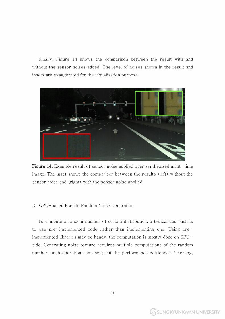
Finally, Figure 14 shows the comparison between the result with and

without the sensor noises added. The level of noises shown in the result and

insets are exaggerated for the visualization purpose.

Figure 14. Example result of sensor noise applied over synthesized night-time

image. The inset shows the comparison between the results (left) without the

sensor noise and (right) with the sensor noise applied.

D. GPU-based Pseudo Random Noise Generation

To compute a random number of certain distribution, a typical approach is

to use pre-implemented code rather than implementing one. Using pre-

implemented libraries may be handy, the computation is mostly done on CPU-

side. Generating noise texture requires multiple computations of the random

number, such operation can easily hit the performance bottleneck. Thereby,

32

we attempted to compute the Poisson random number in GPU to overcome the

performance bottleneck.

Instead of re-implementing the Poisson distribution algorithm from the

scratch, we used the same code implemented in the Standard Template

Library (STL) for the C++ programming language. Specifically, we used

Microsoft’s STL implementation as they are shared as open-source [43].

Although GPU does not provide a random number generator (RNG) without

the usage of an external library (i.e., CUDA), we attempted to implement

pseudo RNG in GPU.

Up-to-date GPU-based implementations of pseudo RNG that are publicly

shared are only designed for a single-use. The most common approach is to

use the texture coordinate as an input, the same random number is returned

for the same texture coordinate. Such an issue can simply overcome by

modifying the input during the computation of a random number; returned

input can be reused for another random number. Moreover, random offset for

each noise texture is given from the CPU-side for additional randomness.

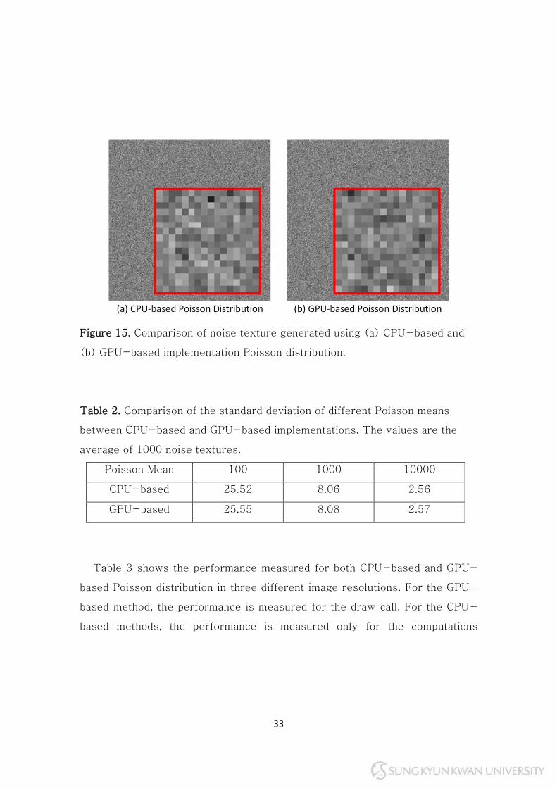
To verify our GPU-based implementation of Poisson distribution with

pseudo RNG, we compared ours with the CPU-based implementation. Figure

15 shows the example result of noise texture generated using the CPU-based

and GPU-based Poisson distribution. Table 2 shows the measurement of the

standard deviation of all pixel values in the noise texture, computed through a

histogram. The differences in standard deviation between the CPU-based and

GPU-based implementation were less than 0.02 for different Poisson means.

33

Figure 15. Comparison of noise texture generated using (a) CPU-based and

(b) GPU-based implementation Poisson distribution.

Table 2. Comparison of the standard deviation of different Poisson means

between CPU-based and GPU-based implementations. The values are the

average of 1000 noise textures.

Poisson Mean 100 1000 10000

CPU-based 25.52 8.06 2.56

GPU-based 25.55 8.08 2.57

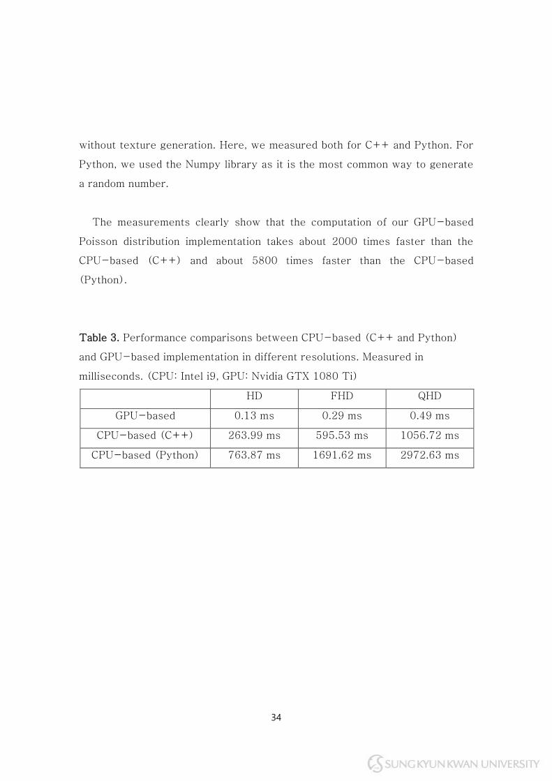
Table 3 shows the performance measured for both CPU-based and GPU-

based Poisson distribution in three different image resolutions. For the GPU-

based method, the performance is measured for the draw call. For the CPU-

based methods, the performance is measured only for the computations

34

without texture generation. Here, we measured both for C++ and Python. For

Python, we used the Numpy library as it is the most common way to generate

a random number.

The measurements clearly show that the computation of our GPU-based

Poisson distribution implementation takes about 2000 times faster than the

CPU-based (C++) and about 5800 times faster than the CPU-based

(Python).

Table 3. Performance comparisons between CPU-based (C++ and Python)

and GPU-based implementation in different resolutions. Measured in

milliseconds. (CPU: Intel i9, GPU: Nvidia GTX 1080 Ti)

HD FHD QHD

GPU-based 0.13 ms 0.29 ms 0.49 ms

CPU-based (C++) 263.99 ms 595.53 ms 1056.72 ms

CPU-based (Python) 763.87 ms 1691.62 ms 2972.63 ms

35

Chapter 4. Results

Experiments of the proposed framework in this thesis are performed on a

machine with the Intel i9-7900X 3.31GHz and the Nvidia GTX 1080 Ti. To

demonstrate the results of the proposed framework, Cityscapes, BDD100K

and KITTI datasets were used. For comparison, the BDD100K dataset was

used for the learning-based method [12]. For implementation, we selected

C++ and the OpenGL Application Programming Interface.

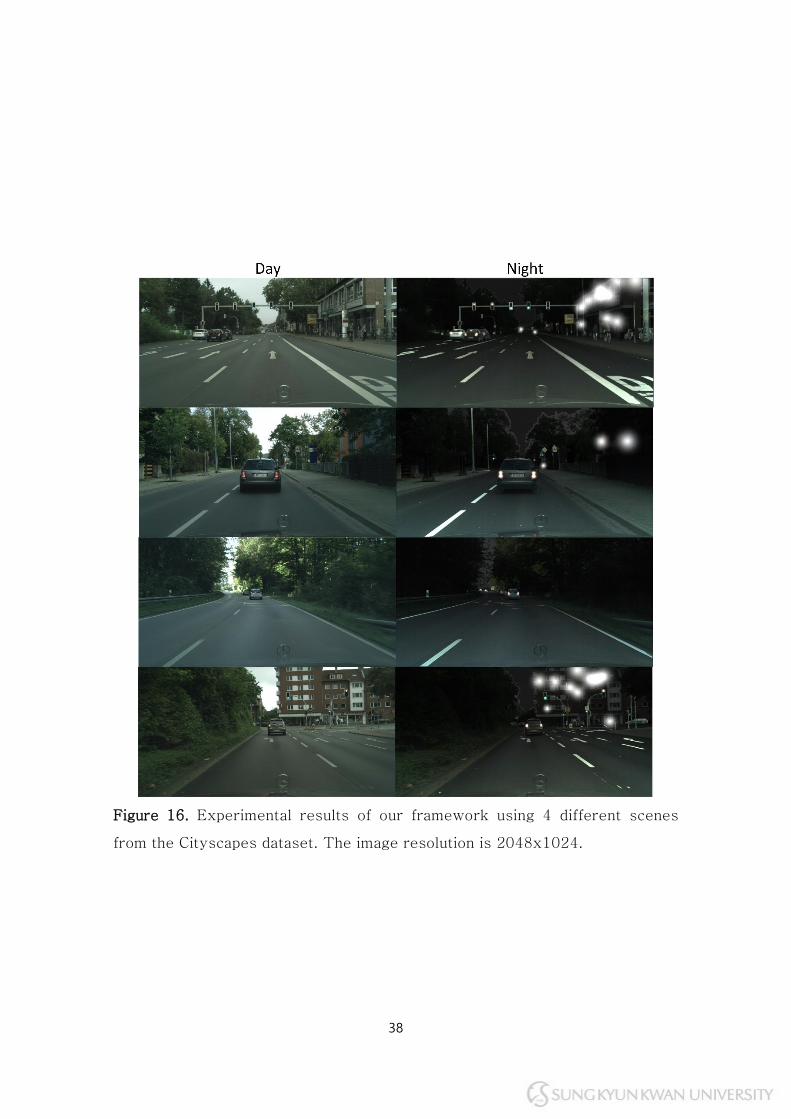
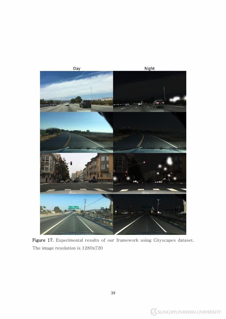
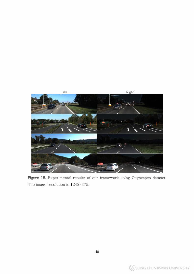
The example results of 3 datasets are shown in Figure 16-18. For the

demonstration, four different day-time road scene images from each dataset

were selected, with corresponding ground truth semantic segmentation images.

The demonstrated results show that our framework is feasible to perform

day-to-night image translation of road scene images without the learning.

The translation is resolution-independent and the results can be easily

adjusted on-the-fly for more plausible results. Moreover, less artifacts are

shown as the proposed framework do not performs unintended translation

during the translation processes.

Figure 19 shows the comparison of results between the proposed

framework and the learning-based method. The results clearly show that our

framework can perform a more plausible day-to-night translation or road

scenes with crisp results in higher-resolution, while the artifacts are yet

observable in the compared method. Figure 20 shows a few detailed

comparisons of results between the proposed framework and the learning-

36

based method. As shown in Figures 20(a), 20(b), 20(d) and 20(c), learning-

based often detects bright area in the scene as a positive light source, while

our results avoid such false estimations. However, as shown in Figures 20(e)

and 20(f), learning-based method tends to do achieve plausible translation in

building windows and street signs than our methods, such areas are not

annotated in our semantic segmentation images. Additional to the qualitative

evaluation as shown in Figures 19 and 20, we computed frechet inception

distance (FID) [44] to further quantitatively evaluate the results between the

proposed framework and the learning-based method. Though FID is originally

designed to evaluate the results of GANs, our method may not fit. Also, the

ground truth images, which are real night-time images of given day-time

images, were cannot be obtained, thus we randomly selected multiple sets of

real night-time images and computed the average FID. Table 4 shows the

average FID; 5 different reference sets compared to our method and the

learning method. Despite that our results produced fewer artifacts in lighting,

and preserved the scene structures better than the results of the learning-

based method, the FID was 13.57 lower than ours. This highly encourages us

to further investigate improving the framework to achieve better FID; more

discussed in the limitation section.

Table 5 shows the comparison of the average time measured for both the

proposed framework and the learning-based method. The proposed

framework shows a nearly real-time solution for a day-to-night translation.

In contrast, the learning-based method, using the same dataset, shows 164

times slower performances. Such performances matter when it comes to

generating a massive dataset. Table 6 shows the average performance

37

breakdown of the proposed framework for each step performed during the

translation. The measurement was performed over three datasets, as shown in

Figure 16-18. Since most steps in our framework operate on GPU-side, the

overall performance for all steps are less than 3 milliseconds, except for the

two: Hough transform and the light map generation.

The overheads in the proposed framework are mostly caused by the CPU-

side operations, rather than the GPU-side operations. The CPU-side

operations in the proposed framework include line detection, vanishing point

detection, and random sampling of light sprite positions. All three overheads

are simply caused by repeated processes; each operation requires multiple

computations. Such overhead may be trivial for a low-resolution image, where

fewer computations are required, but becomes significant for higher-

resolution inputs. To prevent the framework to halt during the translation,

each operation is limited by a certain number with given thresholds. In

practice, such thresholds were never exceeded. The corresponding overheads

can be seen in Table 5.

38

Figure 16. Experimental results of our framework using 4 different scenes

from the Cityscapes dataset. The image resolution is 2048x1024.

39

Figure 17. Experimental results of our framework using Cityscapes dataset.

The image resolution is 1280x720

40

Figure 18. Experimental results of our framework using Cityscapes dataset.

The image resolution is 1242x375.

41

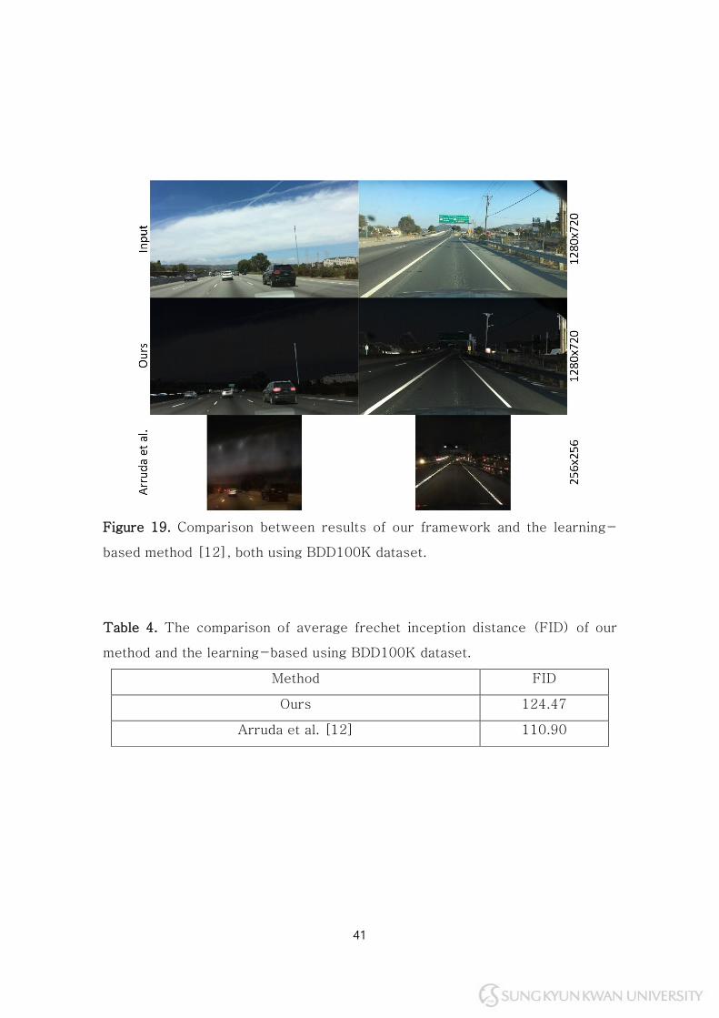
Figure 19. Comparison between results of our framework and the learning-

based method [12], both using BDD100K dataset.

Table 4. The comparison of average frechet inception distance (FID) of our

method and the learning-based using BDD100K dataset.

Method FID

Ours 124.47

Arruda et al. [12] 110.90

42

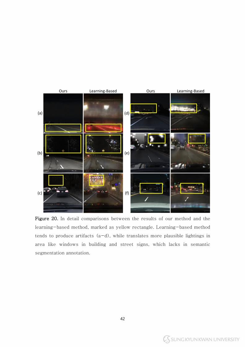
Figure 20. In detail comparisons between the results of our method and the

learning-based method, marked as yellow rectangle. Learning-based method

tends to produce artifacts (a-d), while translates more plausible lightings in

area like windows in building and street signs, which lacks in semantic

segmentation annotation.

43

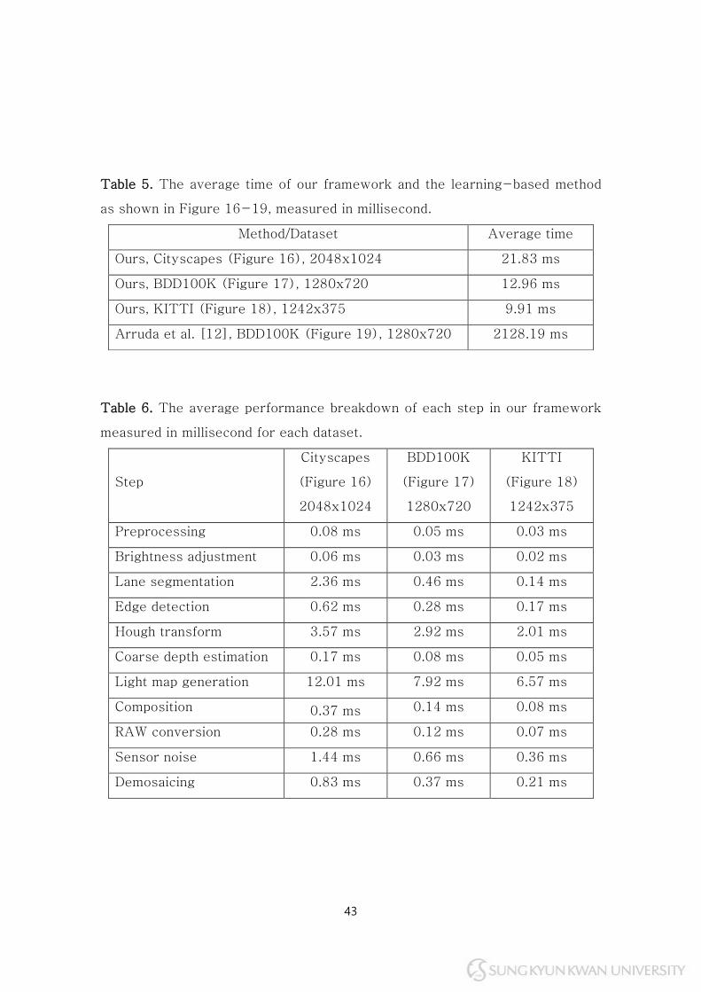
Table 5. The average time of our framework and the learning-based method

as shown in Figure 16-19, measured in millisecond.

Method/Dataset Average time

Ours, Cityscapes (Figure 16), 2048x1024 21.83 ms

Ours, BDD100K (Figure 17), 1280x720 12.96 ms

Ours, KITTI (Figure 18), 1242x375 9.91 ms

Arruda et al. [12], BDD100K (Figure 19), 1280x720 2128.19 ms

Table 6. The average performance breakdown of each step in our framework

measured in millisecond for each dataset.

Step

Cityscapes

(Figure 16)

2048x1024

BDD100K

(Figure 17)

1280x720

KITTI

(Figure 18)

1242x375

Preprocessing 0.08 ms 0.05 ms 0.03 ms

Brightness adjustment 0.06 ms 0.03 ms 0.02 ms

Lane segmentation 2.36 ms 0.46 ms 0.14 ms

Edge detection 0.62 ms 0.28 ms 0.17 ms

Hough transform 3.57 ms 2.92 ms 2.01 ms

Coarse depth estimation 0.17 ms 0.08 ms 0.05 ms

Light map generation 12.01 ms 7.92 ms 6.57 ms

Composition 0.37 ms 0.14 ms 0.08 ms

RAW conversion 0.28 ms 0.12 ms 0.07 ms

Sensor noise 1.44 ms 0.66 ms 0.36 ms

Demosaicing 0.83 ms 0.37 ms 0.21 ms

44

Chapter 5. Conclusion

In this thesis, the author presented a framework for the day-to-night

image translation of the road scene images, using the semantic annotations

from the semantic segmentation.

In contrast to previous learning-based methods, the proposed framework

does not learn to translate the image in order to prevent previous issues

where the desired dataset for the training becomes insufficient, and the

outputs being unpredictable with artifacts. As our framework utilizes the

semantic annotations, we were able to perceive the given scene, perform the

per-element adjustment, and also extract features from the selected scene

elements to synthesize a more plausible night-time image. Besides, the

sensor noises were modeled to obtain even more plausible results.

As demonstrated in the results, the proposed framework successfully

translated the day-time road scene image to the night-time image without

learning. In contrast to learning-based methods, our framework preserved the

input image resolution, which can further be resized for other potential usages.

Thus, the crispness of scene structures was kept. Also, the artifacts were

avoided by not performing unintended translation; visually plausible results

were obtained. Moreover, the overall performance was improved by operating

the most part of the framework in GPU, it shows viable extension for the

application, such as massive dataset generation.

45

Chapter 6. Limitations and Future Work

As our framework utilizes the semantic annotations during the translation,

the semantic segmentation is necessary for prior. Thus, the application of our

framework is limited only to the image with the semantic segmentation. The

annotating process is known to require time and manual effort, not every

dataset provides one and may not be an optimal solution. In the future, we

would like to further extend our framework to integrate a deep neural network

(DNN) model of semantic segmentation. The state-of-the-art models [45,

46] show high performance in pixel-level semantic labeling, yet may have

false labeling; further works are necessary.

Another limitation is the estimation of the coarse depth, which is based on

the single vanishing point. The road scene can be complex, multiple vanishing

points may exist in a single image. The proposed framework currently only

detects a single vanishing point; the estimated coarse depth can be irrelevant

for the images with multiple vanishing points. Hence, our future work includes

further improvement to detect more than one vanishing point not only for a

better estimation of depth but also to enhance overall feature extraction.

Also, the methods that the proposed framework uses to estimate the

lightings are inaccurate. Our results lack optical effects (i.e. lens flare), only

the diffraction-like effect was simply simulated by the bloom effect. Also,

geometries of scene elements are unknown; it is difficult to add plausible light

46

reflection between the objects and the lights. Moreover, randomly splatted

light sprites cause temporal incoherence between the frame to frame, where

the positions of light sprites vary and not being continuous in the image

sequence. As a consequence, further investigation is required for estimating

and simulating lights in the night scene image; our future work includes the

following issues. First, we will train the DNN semantic segmentation model (as

mentioned earlier) with several additional labels (i.e. window, street lights,

etc). Thereby, we segment the areas in the image where it could potentially

be a light source during the night; we expect to achieve better estimations in

lightings than randomly splatting the light sprite. Moreover, we will enhance

our feature extractions to estimate coarse 3D geometries in the image to

simulate better optical effects, such as point-light reflections. Overall, we

seek that proposed framework to achieve both qualitatively and quantitatively

improved than as current.

Additionally, our framework only performs day-to-night translation,

cannot translate the night-time image to the day-time image. The proposed

method may not be suitable for night-to-day image translation. Night-time

images lack much information compared to the day-time image due to the lack

of illumination. Such uneven conditions not only are difficult to obtain high-

performance semantic segmentation but also hard to reproduce the original

color of the scene or translate the overall lightings.

Lastly, we would like to further improve our framework by fully automating

the entire processes, and extend our work to evaluate in deep learning tasks

such as object detection.

47

References

[1] Buades, Antoni, Bartomeu Coll, and J-M. Morel. "A non-local algorithm

for image denoising." 2005 IEEE Computer Society Conference on Computer

Vision and Pattern Recognition (CVPR'05). Vol. 2. IEEE, 2005.

[2] Welsh, Tomihisa, Michael Ashikhmin, and Klaus Mueller. "Transferring

color to greyscale images." Proceedings of the 29th annual conference on

Computer graphics and interactive techniques. 2002.

[3] Pitie, Francois, Anil C. Kokaram, and Rozenn Dahyot. "N-dimensional

probability density function transfer and its application to color transfer."

Tenth IEEE International Conference on Computer Vision (ICCV'05) Volume 1.

Vol. 2. IEEE, 2005.

[4] Reinhard, Erik, et al. "Color transfer between images." IEEE Computer

graphics and applications 21.5 (2001): 34-41.

[5] Shi, Jianbo, and Jitendra Malik. "Normalized cuts and image segmentation."

IEEE Transactions on pattern analysis and machine intelligence 22.8 (2000):

888-905.

[6] Goodfellow, Ian, et al. "Generative adversarial nets." Advances in neural

information processing systems. 2014.

[7] Isola, Phillip, et al. "Image-to-image translation with conditional

adversarial networks." Proceedings of the IEEE conference on computer

vision and pattern recognition. 2017.

48

[8] Zhu, Jun-Yan, et al. "Unpaired image-to-image translation using cycle-

consistent adversarial networks." Proceedings of the IEEE international

conference on computer vision. 2017.

[9] Luan, Fujun, et al. "Deep photo style transfer." Proceedings of the IEEE

Conference on Computer Vision and Pattern Recognition. 2017.

[10] Pathak, Deepak, et al. "Context encoders: Feature learning by inpainting."

Proceedings of the IEEE conference on computer vision and pattern

recognition. 2016.

[11] Choi, Yunjey, et al. "Stargan: Unified generative adversarial networks for

multi-domain image-to-image translation." Proceedings of the IEEE

conference on computer vision and pattern recognition. 2018.

[12] Antipov, Grigory, Moez Baccouche, and Jean-Luc Dugelay. "Face aging

with conditional generative adversarial networks." 2017 IEEE international

conference on image processing (ICIP). IEEE, 2017.

[13] Arruda, Vinicius F., et al. "Cross-domain car detection using

unsupervised image-to-image translation: From day to night." 2019

International Joint Conference on Neural Networks (IJCNN). IEEE, 2019.

[14] Liu, Ming-Yu, Thomas Breuel, and Jan Kautz. "Unsupervised image-to-

image translation networks." Advances in neural information processing

systems. 2017.

[15] Huang, Sheng-Wei, et al. "Auggan: Cross domain adaptation with gan-

based data augmentation." Proceedings of the European Conference on

Computer Vision (ECCV). 2018.

[16] Jiang, Liming, et al. "TSIT: A Simple and Versatile Framework for

Image-to-Image Translation." arXiv preprint arXiv:2007.12072 (2020).

49

[17] Meng, Yingying, et al. "From night to day: GANs based low quality image

enhancement." Neural Processing Letters 50.1 (2019): 799-814.

[18] Sun, Lei, et al. "See clearer at night: towards robust nighttime semantic

segmentation through day-night image conversion." Artificial Intelligence and

Machine Learning in Defense Applications. Vol. 11169. International Society

for Optics and Photonics, 2019.

[19] Anoosheh, Asha, et al. "Night-to-day image translation for retrieval-

based localization." 2019 International Conference on Robotics and Automation

(ICRA). IEEE, 2019.

[20] Cordts, Marius, et al. "The cityscapes dataset for semantic urban scene

understanding." Proceedings of the IEEE conference on computer vision and

pattern recognition. 2016.

[21] Alhaija, Hassan Abu, et al. "Augmented reality meets computer vision:

Efficient data generation for urban driving scenes." International Journal of

Computer Vision 126.9 (2018): 961-972.

[22] Yu, Fisher, et al. "BDD100K: A diverse driving dataset for heterogeneous

multitask learning." Proceedings of the IEEE/CVF Conference on Computer

Vision and Pattern Recognition. 2020.

[23] Ayieko, Charles Opiyo, et al. "Controlled texturing of aluminum sheet for

solar energy applications." Advances in Materials Physics and Chemistry 5.11

(2015): 458.

[24] Namba, Yoshiharu, and Hideo Tsuwa. "Surface properties of polished

stainless steel." CIRP Annals 29.1 (1980): 409-412.

[25] Sielachowska, M., and M. Zajkowski. "Assessment of Light Pollution

Based on the Analysis of Luminous Flux Distribution in Sports Facilities."

Engineer of the XXI Century. Springer, Cham, 2020. 139-150.

50

[26] Mendenhall, Michael J., Abel S. Nunez, and Richard K. Martin. "Human

skin detection in the visible and near infrared." Applied optics 54.35 (2015):

10559-10570.

[27] Störring, Moritz. Computer vision and human skin colour. Diss. Computer

Vision & Media Technology Laboratory, Faculty of Engineering and Science,

Aalborg University, 2004.

[28] Govender, Megandhren, K. Chetty, and Hartley Bulcock. "A review of

hyperspectral remote sensing and its application in vegetation and water

resource studies." Water Sa 33.2 (2007).

[29] Jones, Amy, et al. "An advanced scattered moonlight model for Cerro

Paranal." Astronomy & Astrophysics 560 (2013): A91.

[30] Singh, Pankaj Pratap, and R. D. Garg. "Study of spectral reflectance

characteristics of asphalt road surface using geomatics techniques." 2013

International Conference on Advances in Computing, Communications and

Informatics (ICACCI). IEEE, 2013.

[31] Batista, Marcos Paulo, et al. "Lane detection and estimation using

perspective image." 2014 Joint Conference on Robotics: SBR-LARS Robotics

Symposium and Robocontrol. IEEE, 2014.

[32] Canny, John. "A computational approach to edge detection." IEEE

Transactions on pattern analysis and machine intelligence 6 (1986): 679-698.

[33] Hough, Paul VC. "Method and means for recognizing complex patterns."

U.S. Patent No. 3,069,654. 18 Dec. 1962.

[34] Ester, Martin, et al. "A density-based algorithm for discovering clusters

in large spatial databases with noise." Kdd. Vol. 96. No. 34. 1996.

51

[35] Boonsim, Noppakun, and Simant Prakoonwit. "An algorithm for accurate

taillight detection at night." International Journal of Computer Applications

(2014).

[36] Kuo, Ying-Che, and Hsuan-Wen Chen. "Vision-based vehicle detection

in the nighttime." 2010 International Symposium on Computer, Communication,

Control and Automation (3CA). Vol. 2. IEEE, 2010.

[37] Kafai, Mehran, and Bir Bhanu. "Dynamic Bayesian networks for vehicle

classification in video." IEEE Transactions on Industrial Informatics 8.1

(2011): 100-109.

[38] Aguerrebere, Cecilia, et al. "Study of the digital camera acquisition

process and statistical modeling of the sensor raw data." (2013).

[39] Chen, Junqing, et al. "Digital camera imaging system simulation." IEEE

Transactions on Electron Devices 56.11 (2009): 2496-2505.

[40] Gow, Ryan D., et al. "A comprehensive tool for modeling CMOS image-

sensor-noise performance." IEEE Transactions on Electron Devices 54.6

(2007): 1321-1329.

[41] Bielova, Oleksandra, et al. "A Digital Image Processing Pipeline for

Modelling of Realistic Noise in Synthetic Images." Proceedings of the IEEE

Conference on Computer Vision and Pattern Recognition Workshops. 2019.

[42] Hibbard, Robert H. "Apparatus and method for adaptively interpolating a

full color image utilizing luminance gradients." U.S. Patent No. 5,382,976. 17

Jan. 1995.

[43] Microsoft. “Microsoft/STL.” GitHub, github.com/microsoft/STL.

[44] Heusel, Martin, et al. "Gans trained by a two time-scale update rule

converge to a local nash equilibrium." Advances in neural information

processing systems. 2017.

52

[45] Tao, Andrew, Karan Sapra, and Bryan Catanzaro. "Hierarchical Multi-

Scale Attention for Semantic Segmentation." arXiv preprint arXiv:2005.10821

(2020).

[46] Wang, Jingdong, et al. "Deep high-resolution representation learning for

visual recognition." IEEE transactions on pattern analysis and machine

intelligence (2020).

53

논문요약

의미적 분할을 이용한 낮에서 밤으로 도로 환경

사진 변환 기법

Seung Youp Baek

소프트웨어학과

성균관대학교

Day-to-night 이미지 변환은 주어진 낮 시간대 영역(domain)의 사진을 밤

시간대 영역의 사진으로 변환하는 작업을 말한다. 최근 연구들은 낮 시간대의 도로

환경 데이터셋을 밤 시간대로 변환하는 학습 기반의 기법들을 소개하였고,

계속해서 발전된 결과들을 보여주었다. 그러나 학습 기반의 기법들은 일반적으로

예측이 불가능하기 때문에 원하는 결과를 얻기 어려운 경우가 많다. 또한, 원하는

주석(annotation)이 있는 데이터셋들은 사용하기에 불충분하거나 얻을 수 없을

수도 있다. 이에 본 연구는 도로 환경 사진에 day-to-night 이미지 변환 기법을

수행하는 반자동 프레임워크를 제안한다. 이전의 접근 방식과는 달리, 본 연구는

이미지 변환을 위해 학습을 하지 않는다. 대신해서 본 연구는 의미적

분할(semantic segmentation)로 얻는 의미적 주석(semantic annotation)들을

활용하여 주어진 환경을 이해한다. 의미적 주석의 활용으로, 사진 속 요소별 변환과

조절을 수행하여 더욱 실제 같은 밤 사진을 생성한다. 이어서, 사진 속 간단한

심도나 빛을 추정하는 데 있어 의미적 주석을 활용하여 의도하지 않은 변환을

피하고 전체적인 견고성을 높인다. 마지막으로, 이미지 센서 노이즈를 모델링하고

시뮬레이션하여 더욱 그럴듯한 결과물을 얻는다. 결과적으로, 본 연구가 제시하는

54

프레임워크의 실험적 결과가 보여주듯이, 본 연구의 프레임워크는 더욱 그럴듯한

고해상도의 밤 사진을 생성할 뿐만 아니라, 학습 기반의 기법에서 나타나는 무작위

아티팩트들을 피한다. 게다가, 본 연구의 프레임워크는 대부분 GPU로 구동되기

때문에 결과를 실시간에 가깝게 얻을 수 있으며, 이는 데이터셋 생성을 위한 확장

가능성도 보여준다.

주제어: 영상 처리, 계산 사진학, 낮에서 밤, 의미적 분할, GPU

Maste

r’s

Thesis

Road S

cene Im

age T

ransla

tion fro

m D

ay to

Nig

ht

usin

g S

em

antic

Segm

enta

tion

2

0

2

1

S

eung Y

oup B

aek