Roadside Passive Multichannel Analysis of Surface Waves (MASW)

Park, C.B.* and Miller, R.D.

+

*Formerly,

+

Kansas Geological Survey, University of Kansas, 1930 Constant Avenue,

Lawrence, Kansas 66047-3726

choonpark@gmail.com (Park, corresponding author) (Tel: 785-864-2162)

rmiller@kgs.ku.edu (Tel: 785-864-2091)

March 5, 2007 (resubmitted)

Abstract

For the most accurate results, a 2D receiver array such as a cross or circular type

should be used in a passive surface wave survey. It is often not possible to secure such a

spacious area, however, especially if the survey has to take place in an urban area. A

passive version of the multichannel analysis of surface waves (MASW) method is

described that can be implemented with the conventional linear receiver array deployed

alongside a road. Offline, instead of inline, nature of source points on the road is

accounted for during dispersion analysis by scanning recorded wavefields through 180-

degree azimuth range to separate wavefields from different azimuths and propagated with

different phase velocities. Then, these wavefields are summed together along the

azimuth axis to yield the azimuth-resolved phase velocity information for a given

frequency. In addition, it is also attempted to account for cylindrical, instead of planar,

nature of surface wave propagation that often occurs due to the proximity of source

points by considering the distance between a receiver and a possible source point.

Performance of the processing schemes is compared to that of the scheme that accounts

for inline propagation only. Comparisons made with field data sets showed that the latter

scheme resulted in overestimation of phase velocities up to 30 percent, whereas the

overestimation could be reduced to less than 10 percent if these natures are accounted for

according to the proposed schemes. They also showed the overestimation can increase

with distance between the road and the receiver line.

Introduction

As the active survey mode often does not achieve sufficient depth of

investigation, the passive surface wave method seems an alternative. In addition, as the

necessity of surveys inside urban areas grows, utilizing those surface waves generated by

local traffic is deemed to be a fascinating choice recently (Asten, 1978; Louie, 2001;

Okada, 2003; Suzuki and Hayashi, 2003; Yoon and Rix, 2004; Park et al., 2004).

Although this type of surface wave application had come under study nearly a half-

century ago in Japan under the name of Microtremor Survey Method (MSM) (Aki, 1957;

Tokimatsu, et al., 1992), it was not well known among relevant communities in Western

countries until quite recently, with the exception of a few study groups (Asten, 1978;

Asten and Henstridge, 1984). Spatial Autocorrelation (SPAC) (Aki, 1957) and f-k

methods were commonly used to process passive surface waves for dispersion analysis.

More recently, an imaging method similar to the one used in the active method was

developed (Park et al., 2004; 2007).

Furthermore, because the true 2D receiver array such as a cross layout is not a

practical or possible mode of survey in urban areas populated with buildings, a method

that can be implemented with the conventional 1D linear receiver array should get its

own credit in any case (Louie, 2001). The underlying assumption with such a 1D method

lies in the nature of wave propagation which is the same inline propagation as in the case

of an active survey. Subsequent data processing for dispersion analysis is therefore a 1D

scheme considering only those waves propagating parallel to (inline with) the linear

receiver line.

In the case of a passive survey alongside a road, points of surface wave generation

are usually on the road since waves are generated when moving vehicles travel onto

irregularities on the road. Because the receiver line is always off the road, the wave

propagation is therefore hardly in accordance with the inline propagation although being

close to it when sources are at far distances. If those strong waves from nearby source

points dominate and their offline nature is not accounted for during the dispersion

analysis, phase velocities are overestimated approximately in inverse proportion to the

cosine of the azimuth (cos). Furthermore, considering relatively strong energy from

nearby source points, the dominating mode of propagation may be not only offline but

also cylindrical with a wavefront whose curvature cannot be ignored.

Ways to account for these offline and cylindrical characteristics are described

with results compared to those from the conventional analysis scheme based on the inline

plane wave propagation. Fundamentals of data acquisition and processing techniques

have evolved from the multichannel analysis of surface waves (MASW) method (Park et

al., 1999) for active surface wave surveys. The offline nature is accounted for by a

scheme (Park et al., 2004) that scans through a possible range (180 degrees) of incoming

azimuths of dominating waves for each frequency component of the dispersion analysis.

Then, all the energy in this phase velocity-azimuth space is stacked (summed) along the

azimuth () axis to account for multiple energy peaks that may represent different modes

and sources. It has been attempted to account for the cylindrical nature by an additional

scheme that calculates the approximate distance between a specific receiver and a

possible source point, which is in turn determined from the consideration of azimuth and

approximate distance between the receiver line and the road. It is shown that these

proposed schemes can correct for the overestimation to some degree but not completely,

indicating that a true 2D array has to be used for the most accurate estimation. The

incomplete correction becomes more significant for longer wavelengths. Tests with field

data sets show the overestimation caused by the conventional inline processing can be as

large as 30 percent, whereas the overestimation can be reduced to less than 10 percent by

using the proposed schemes.

Roadside Passive Surface Waves

Three different types of wave propagation can exist: inline plane (IP), offline

plane (OP), and offline cylindrical (OC) propagations (Figure 1). Propagation of waves

generated from distant points on the surveying road (for example, at a distance 10 times

or more array lengths) can be an example of the IP type if the road is fairly straight in the

corresponding segment (Figure 1a). On the other hand, if the road turns or there are other

roads around the surveying area, there can be waves generated at far distances

approaching the receiver line with a significant azimuthal angle making an example of

the OP type (Figure 1b). Furthermore, source points on the surveying road can be close

to the array (for example, at a distance shorter than a few times array length from either

end or even within the receiver line), making an example of the OC type (Figure 1c).

Waves of OC type propagate into the receiver line with a significant curvature due to the

proximity and the offline nature. A considerable amount of recorded energy can be of

this origin due to the proximity of the major source points.

The IP waves will make a straight linear arrival pattern on the recorded data with

a slope (S= dt/dx) the same as the inverse of the phase velocity (1/c) (i.e., slowness) for a

particular frequency (f) (Figure 2). The OP waves will also make a straight linear arrival

pattern but with its slope always smaller than that (1/c) of the IP case by a ratio of cosine

of the azimuth (cos) (Park et al., 2004). Then, its corresponding velocity (dx/dt) will be

overestimated by a ratio of 1/cos if the offline nature is not properly accounted for. The

arrival pattern of the OC waves will be hyperbolic with an asymptote the same as that of

the OP for the same azimuth ().

Schemes for Dispersion Imaging

Dispersion imaging schemes to deal with each of these types of propagation are

described. It is assumed that the road runs along the horizontal axis (x) with the receiver

line in parallel to it with a certain vertical separation (dy) (Figure 3).

Inline Plane (IP) Waves

IP waves are the simplest type from the data processing perspective. They can be

processed by any scheme commonly used for active surveys. With the scheme by Park et

al. (1998; 2004), to calculate the relative energy, E

IP

(,c), for a particular frequency

(=2f) and a scanning phase velocity (c) in the dispersion image, it first applies the

necessary phase shift (

i

=x

i

/c) to the Fourier transformation, R

i

(), of the i-th trace,

r

i

(t), at offset x

i,

sums all (N) phase-shifted traces, and then takes the absolute value of the

summed complex number:

N

i

i

j

N

i

i

j

IP

ReRecE

ii

11

)()(),(

(1)

To account for the possible bidirectional nature of the incoming waves from both ends of

the receiver array, the step of phase shift followed by the summation is repeated by

changing the sign of the phase shift in the above equation. A method by Louie

(2001)commonly known as the refraction microtremor (ReMi) methodis based on

this algorithm by assuming that the major part of the recorded waves are of IP type and

any other offline waves of significant energy, if they exist, should appear at higher phase

velocities. It therefore tries to extract a curve by following a trend of lowest phase

velocity in the energy band of dispersion in the space of E

IP

(,c). With this method,

however, the consideration of the inherent banding effect due to the limited spatial

coverage of the measurement is not properly accounted for.

Figure 4 shows processing results obtained by using the above equation (1) when

applied to synthetic 24-channel records generated from an inline source (S0) marked in

Figure 3 by using the modeling scheme by Park and Miller (2005). A dispersion curve

with an arbitrary constant phase velocity of 500 m/sec was used during the modeling. The

effect of using different receiver array lengths is also noticeable from the overall

thickness of the banded (instead of thin-line) image changing with total length of the

receiver line. This modeling with a perfectly inline source illustrates the inherent band

appearance of the image resulting from a processing scheme applied to finite lengths in

time (t) and space (x). Width of the band also changes with wavelength for a given

length of the receiver line.

Offline Plane (OP) Waves

OP waves can be processed by any algorithm based on the conventional 2D

wavenumber (k

x

-k

y

) method (Lacoss et al., 1969; Capon, 1969). The method by Park et

al. (2004) modifies the traditional method in such a way that the possible multi-modal

nature of dispersion can be imaged in an intuitive manner by stacking energy in the 2D

wavenumber space along the azimuth axis. This method therefore adds another

parameter for scanning in comparison to (1): the azimuth (). For each frequency (),

the energy, E

OP

(,c,), for a scanning phase velocity (c) is calculated by assuming an

azimuth (). This calculation is then carried over the scanning range of the phase

velocity (for example, 50 m/sec-3000 m/sec with 5-m/sec increment), and then over that

of the azimuth (for example, 0-180 degrees in 5-degree increments):

)1800(for )(),,(

1

,

θ RecE

N

i

i

j

OP

i

(2)

For given c and , the necessary phase shift

,i

=-x

i

cos/c for a trace at x

i

is calculated

based on the projection principle (Park et al., 2004). Here the scanning range of azimuth

() is only within the two quadrants (180 degrees) due to the linear nature of the receiver

line. All the IP waves that exist are handled in a correct manner as they are detected

during the scanning of azimuth near 0 and 180 degrees, respectively.

In the space of c and for a given , there can be multiple energy peaks

occurring at different phase velocities and azimuths, representing different modes and

sources, respectively. Also, different amplitudes of these peaks can represent different

energy partitioning between modes or different strengths of the source or both. To fully

account for all these possibilities, all the energy in c- space is stacked (summed) along

the azimuth () axis for N

different azimuths to produce E

OP

(, c):

N

i

iOPOP

cEcE

1

),,(),(

(3)

that will constitute in the final disperion-image space one energy line at a particluar

frequency, , showing the variation with different phase velocities.

Offline Cylindrical (OC) Waves

OC waves are processed in a similar manner to the OP waves, (2) and (3), only

with an additional consideration of the finite, rather than infinite, distance (l

, i

) between

the source point (x

, y

) and each receiver point (x

i

) for a scanning angle (Figure 5):

2

2

,

yxxl

ii

(with x

= y

/ tan and y

= dy) (4)

Then, the phase shift term in equation (2) is determined as

,i

=-l

,i

/c. The distance, l

,i

,

obviously can change as the road itself has its own width and irregularities may exist

anywhere on the road. An extensive modeling experiment indicated that the exact

distance, however, is not critical and that the distance between the center of the road and

the receiver line is usually sufficient enough to account for the curvature in the arrival

pattern of the OC waves. This scheme processes the IP waves correctly as it becomes

identical to that for the IP waves for grazing azimuthal angles (close to 0 or 180 degrees).

OP waves (for example, waves from other nearby roads) can also be processed by this

scheme, only with a slightly reduced sensitivity.

Synthetic Data Testing of Offline Schemes

All these three schemes are tested on synthetic data sets. A modeling scheme

introduced in Park and Miller (2005) was used to generate synthetic records (not shown)

of 24-channel acquisition with a linear receiver array of 2-meter spacing (Figure 3).

Three different source points (S1, S2, and S3) were separately modeled that had azimuths

of =15, 30, and 45 with the same inline offset of 4-meter (x

1

= 4 m) with

corresponding offline offsets (dy’s) of approximately 7 m, 15 m, and 27-m, respectively.

A constant phase velocity of 500 m/sec was used for a frequency band of 5-100 Hz,

giving an average wavelength () of about 50 m. Attenuation of near-surface materials

was accounted for by including a Q-factor of 30 as a frequency-dependent energy

modulation factor of surface waves in addition to the cylindrical divergence term.

Although all the modeled source points were offline, the inline processing scheme of (1)

was also applied for a comparison purpose. Figure 6 shows processing results from all

these schemes. The modeled phase velocity of 500 m/sec has been indicated by a straight

dotted line in the figures. Those curves extracted from the amplitude peaks in the

dispersion images also have been superimposed.

Results from the IP scheme show the imaged phase velocities being progressively

higher as the azimuth of source point increases (Figures 6a-6c). For relatively large

azimuths ( = 30 and 45), the image trend converges to the theoretical value (=c/cos)

at higher frequencies (for example, > 50 Hz) where corresponding wavelengths become

shorter than the offline offsets (dy’s), whereas it tends to deviate more at lower

frequencies. This non-constant nature of the deviation is therefore due to the different

degrees of proximity for different wavelengths (’s) for a given offline offset (dy).

Performance of the OP scheme (Figures 6d-6f) shows a lesser degree of overestimation,

indicating a correction capacity in comparison to the IP scheme. The results from the OC

scheme (Figures 6g-6i) show the least amount of overestimation in general for all three

source points. None of the three schemes, however, shows complete results without any

deviation from the correct value. The most accurate estimation is obtained through a

survey using a true 2D receiver array followed by data processing using the OP scheme

(Figure 7).

Relative performance of the OC scheme is maximized when the x-coordinate of

an offline source point is within that of the receiver line (intra-line case) as noticed from

another modeling example illustrated in Figure 8. Figure 9 shows the performance

results from a modeling of multiple source points with the same offline distance (dy) of

10 meters. It is noted that the OC scheme gives the most accurate results with marginal

improvement over the OP scheme, whereas results from the IP scheme show the largest

deviation in general trend of the image.

Field Data Example

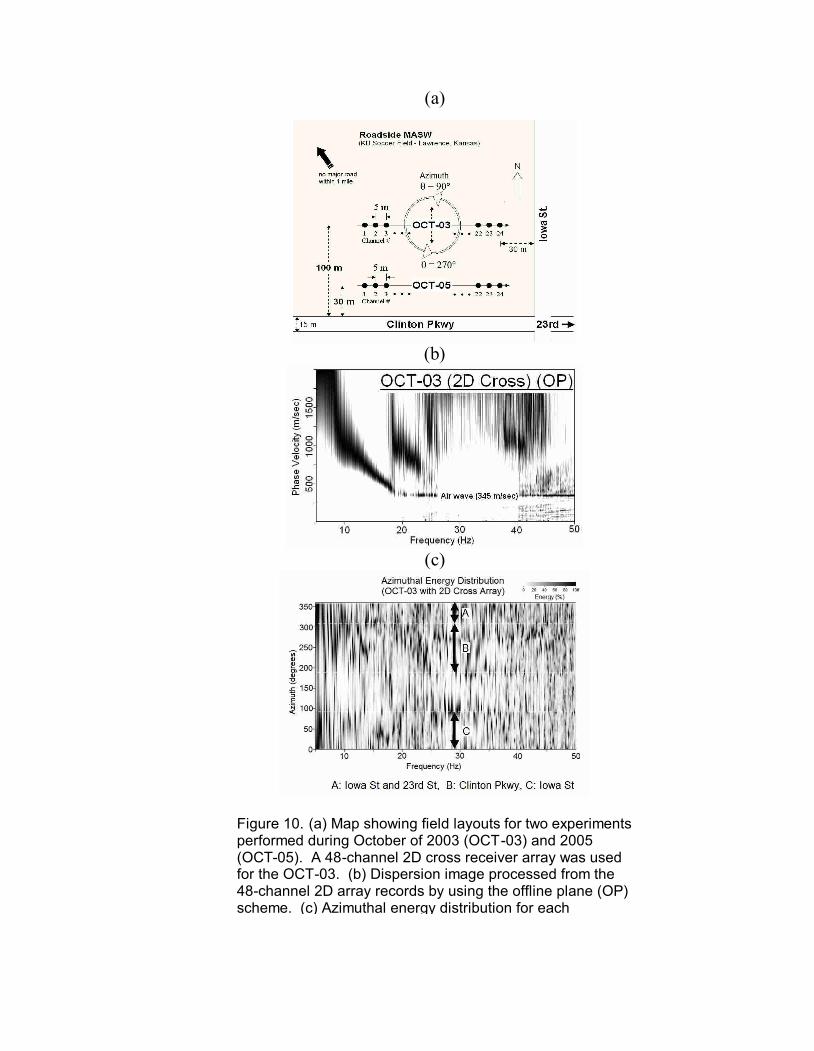
Two sets of field data were used to test these three processing schemes. One data

set (OCT-03) was prepared from the data set acquired in October 2003 (Park et al., 2004)

near a soccer field in Lawrence, Kansas, by using a 2D cross layout of total 48 channels

(Figure 10) with a 5-m receiver spacing. The first 24-channel data that ran East-West (E-

W) in parallel to the Clinton Parkway were taken to mimic a 1D linear array. The

separation (dy) between this receiver line and the center of Clinton Parkway was about

100 meters. For comparison purposes, a dispersion image that was obtained from the full

data set of the 2D cross layout has been displayed in Figure 10b. In addition, an

azimuthal energy distribution, a by-product of the scheme by Park et al. (2004), is

displayed in Figure 10c that shows dominant azimuths for different frequencies analyzed

for the image. The other set of data (OCT-05) was acquired in October 2005 using a 24-

channel linear array directly south of the E-W line used for OCT-03 by using the same

receiver spacing of 5 meters (Figure 10). This line was about 30 meters from the road (dy

= 30 m).

Ten individual records acquired at each survey time were processed using three

different schemes, and their dispersion images were vertically stacked together (to

increase the image resolution) to make the images displayed in Figures 11-12. The

strong major trend of dispersion visible on all images in 8-17 Hz was previously

confirmed as a higher mode (M1), instead of the fundamental mode (M0), through a

combined analysis with an active survey (Park et al., 2005). Dispersion curves were

extracted from the trends by picking maximum points in the energy band with a small

interval (0.01 Hz) and then calculating the best fitting curve through the linear regression

method. All these curves are displayed in Figures 11d and 12d. Curves from the IP

scheme show overestimations in comparison to those from the other two schemes in both

surveys. The amount of overestimation, however, becomes smaller as the receiver array

gets closer to the road. It is also shown that the two offline (OP and OC) schemes

resulted in a certain amount of overestimation for frequencies lower than 12 Hz (for

wavelengths longer than about 75 meters) as noticed when compared to the curve from

the 2D cross layout. Curves from the survey closer to the road show (OCT-05) a slight

difference in general trend, possibly due to a slight difference in near-surface geology in

comparison to the results from the previous survey performed about 70-meters further

away.

Discussions

It was shown through numerical modeling that the OC scheme should give a

superior performance especially when there are some intra-line source points on the road.

Field data examples did not demonstrate this point, as the results from both OP and OC

schemes were almost identical. This indicates that there were not such strong intra-line

source points on the road at the particular location where the surveys were performed.

Azimuthal analysis for major source points in the surveyed area performed with the 2D

(cross and circular) receiver layouts (Park et al., 2004; Park and Miller, 2005) indicated

that major contribution of surface waves came from the 23rd St. close to the intersection

with the Iowa St as seen from Figure 10c. Although the theoretical analysis and

modeling experiments indicated possible improvement of imaging quality with the OC

scheme in comparison to the OP scheme, the further comparative analysis is left for

future research to better understand those influencing conditions not covered in this

paper.

Even if a 2D layout and the subsequent OP scheme are used, overestimation can

still be significant for those long wavelengths comparable to distance to the major source

points as seen from the modeling result shown in Figure 7. This finite (instead of

infinite) nature of the source distance is inherent to the passive surface wave methods

utilizing local traffic noise. The OC scheme was applied only to the linear array, but it

can be extended to a 2D layout.

Conclusions

With a roadside surface wave survey using a linear receiver array, using a 2D

dispersion analysis scheme (despite the 1D nature of data acquisition) that accounts for

the offline nature of the passive surface waves is recommended. In addition, considering

a relatively long receiver array and the possibility of strong surface waves being

generated at nearby points on the road, accounting for the cylindrical nature through a

simple modification of the 2D algorithm to improve the accuracy of the processing is also

recommended.

Acknowledgments

Field experiments were made through careful preparations and precise operations

performed by Brett Wedel, Noah Stimac, Larry Waldron, and Brett Bennett at the Kansas

Geological Survey (KGS). We give our sincere appreciation to them. We also thank

Marla Adkins-Heljeson and Mary Brohammer at KGS for their helps with the manuscript

preparation.

References

Aki, K., 1957, Space and time spectra of stationary stochastic waves, with special reference

to microtremors: Bull. Earthq. Res. Inst., v. 35, p. 415-456.

Asten, M.W., 1978, Geological control on the three-component spectra of Rayleigh-wave

microseisms: Bull., Seism. Soc. Am., v. 68, p. 1623-1636.

Asten, M.W., and Henstridge, J.D., 1984, Array estimators and the use of microseisms for

reconnaissance of sedimentary basins: Geophysics, v. 49, p. 1828-1837.

Capon, J., 1969, High resolution frequency-wavenumber analysis: Proc. Inst. Elect. and

Electron Eng., 57, 1408-1418.

Suzuki, H., and Hayashi, K., 2003, Shallow S-wave velocity sounding using the

microtremors array measurements and the surface wave method; Proceedings of the

SAGEEP 2003, San Antonio, TX, SUR08, Proceedings on CD ROM.

Lacoss, R.T., Kelly, E.J., and Toksöz, M.N., 1969, Estimation of seismic noise structure

using arrays: Geophysics, 34, 21-38.

Louie, J.N., 2001, Faster, better: shear-wave velocity to 100 meters depth from refraction

microtremor arrays; Bulletin of the Seismological Society of America, 2001, 91, (2),

347-364.

Okada, H., 2003, The microtremor survey method; Geophysical Monograph Series, no.

12, published by Society of Exploration Geophysicists (SEG), Tulsa, OK.

Park, C.B., Miller, R.D., Xia, J., and Ivanov, J., 2007, Multichannel analysis of surface waves

(MASW)active and passive methods: The Leading Edge, January.

Park, C.B., Miller, R.D., Ryden, N., Xia, J., and Ivanov, J., 2005, Combined use of active

and passive surface waves: Journal of Engineering and Environmental Geophysics

(JEEG), 10, (3), 323-334.

Park, C.B., Miller, R.D., Xia, J., and Ivanov, J., 2004, Imaging dispersion curves of

passive surface waves: SEG Expanded Abstracts: Soc. Explor. Geophys., (NSG 1.6),

Proceedings in CD ROM.

Park, C.B. and Miller, R.D., 2005, Multichannel analysis of passive surface waves

modeling and processing schemes: Proceedings of the Geo-Frontiers conference,

Austin, Texas, January 23-26, 2005.

Park, C.B., Miller, R.D., and Xia, J., 1999, Multichannel analysis of surface waves

(MASW); Geophysics, 64, 800-808.

Park, C.B., Xia, J., and Miller, R. D., 1998, Imaging dispersion curves of surface waves

on multi-channel record; SEG Expanded Abstracts, 1377-1380.

Suzuki, H, and Hayashi, K., 2003, Shallow s-wave velocity sounding using the Microtremors

array measurements and the surface wave method; Proceedings of the SAGEEP 2003, San

Antonio, Texas, SUR08, Proceedings on CD ROM.

Tokimatsu, K., Shinzawa, K., and Kuwayama, S., 1992, Use of Short-Period Microtremos for

Vs Profiling, Journal of Geotechnical Engineering, ASCE, Vol. 118, No. 10, pp. 1544-

1558.

Yoon, S., and Rix, G., 2004, Combined active-passive surface wave measurements for

near-surface site characterization; Proceedings of the SAGEEP 2004, Colorado

Springs, CO, SUR03, Proceedings on CD ROM.

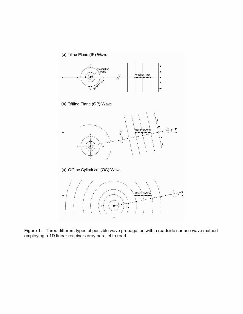
Figure 1. Three different types of possible wave propagation with a roadside surface wave method

employing a 1D linear receiver array parallel to road.

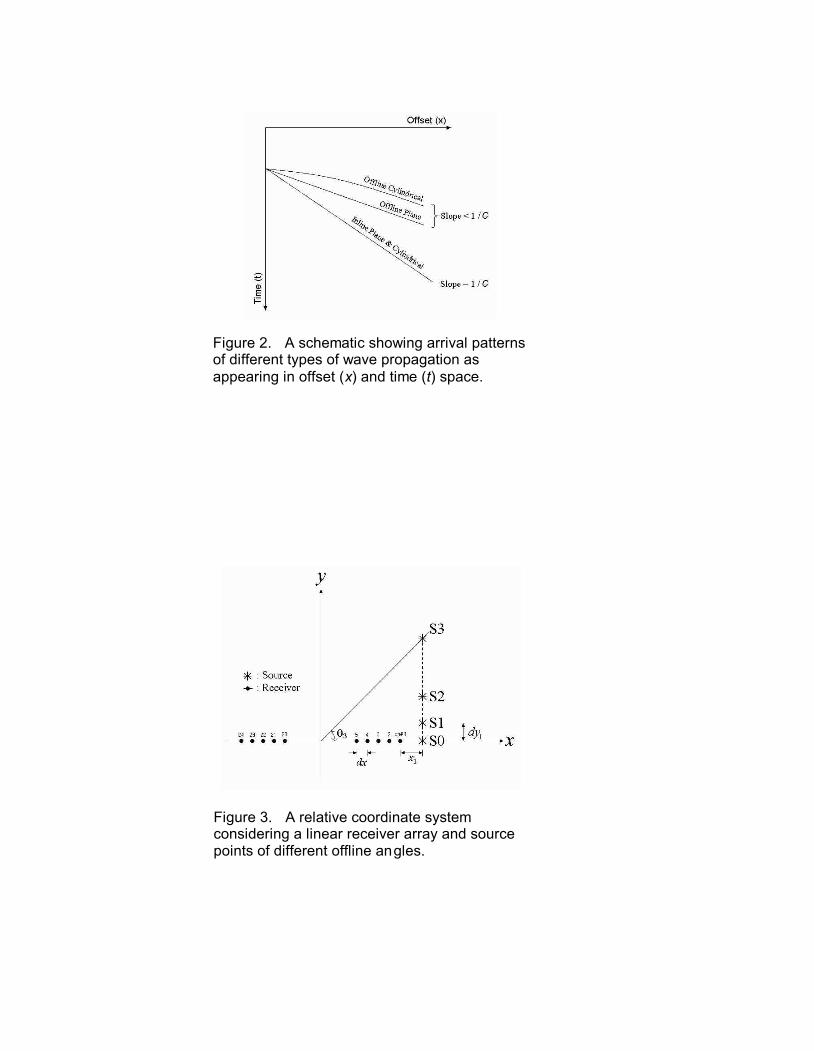
Figure 2. A schematic showing arrival patterns

of different types of wave propagation as

appearing in offset (x) and time (t) space.

Figure 3. A relative coordinate system

considering a linear receiver array and source

points of different offline angles.

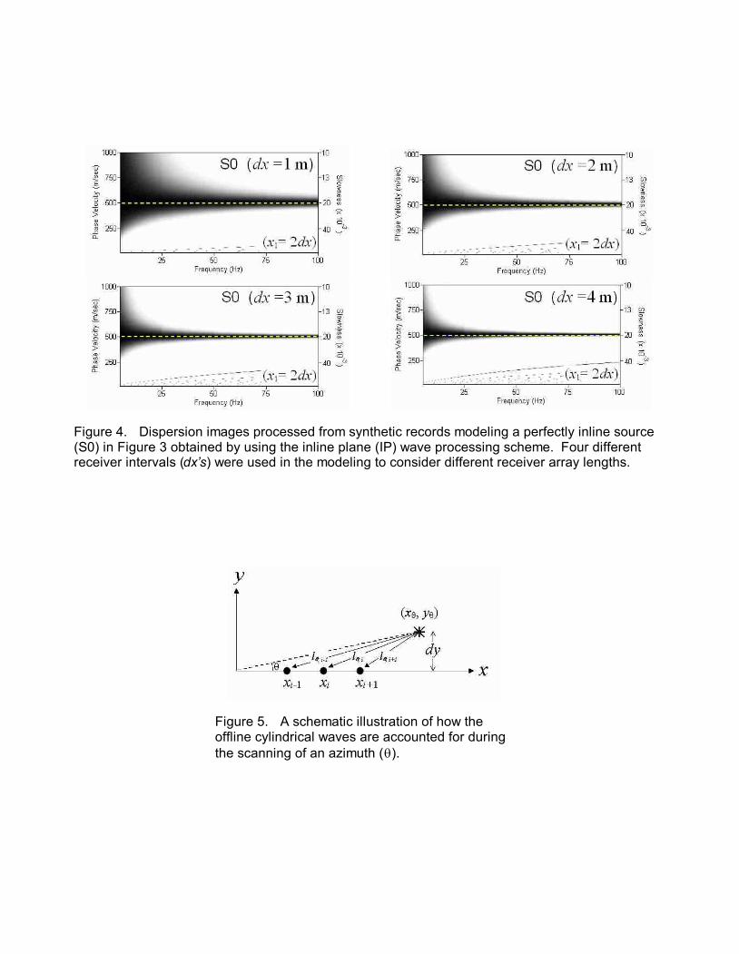
Figure 5. A schematic illustration of how the

offline cylindrical waves are accounted for during

the scanning of an azimuth ().

Figure 4. Dispersion images processed from synthetic records modeling a perfectly inline source

(S0) in Figure 3 obtained by using the inline plane (IP) wave processing scheme. Four different

receiver intervals (dx’s) were used in the modeling to consider different receiver array lengths.

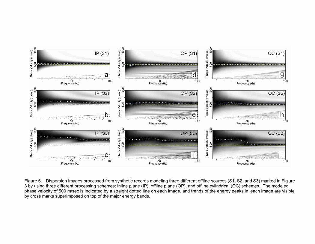
Figure 6. Dispersion images processed from synthetic records modeling three different offline sources (S1, S2, and S3) marked in Fig ure

3 by using three different processing schemes: inline plane (IP), offline plane (OP), and offline cylindrical (OC) schemes. The modeled

phase velocity of 500 m/sec is indicated by a straight dotted line on each image, and trends of the energy peaks in each image are visible

by cross marks superimposed on top of the major energy bands.

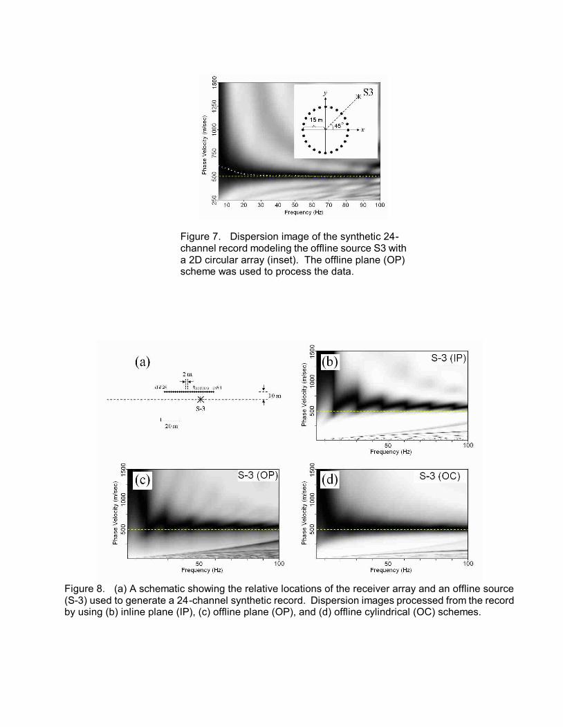
Figure 7. Dispersion image of the synthetic 24-

channel record modeling the offline source S3 with

a 2D circular array (inset). The offline plane (OP)

scheme was used to process the data.

Figure 8. (a) A schematic showing the relative locations of the receiver array and an offline source

(S-3) used to generate a 24-channel synthetic record. Dispersion images processed from the record

by using (b) inline plane (IP), (c) offline plane (OP), and (d) offline cylindrical (OC) schemes.

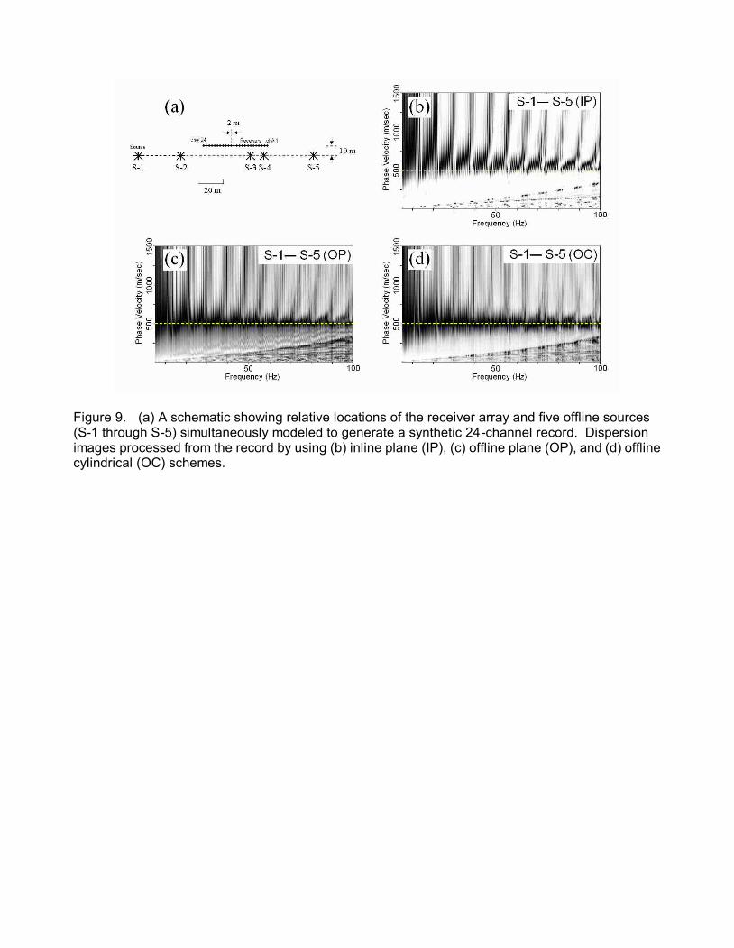
Figure 9. (a) A schematic showing relative locations of the receiver array and five offline sources

(S-1 through S-5) simultaneously modeled to generate a synthetic 24-channel record. Dispersion

images processed from the record by using (b) inline plane (IP), (c) offline plane (OP), and (d) offline

cylindrical (OC) schemes.

(a)

(b)

(c)

Figure 10. (a) Map showing field layouts for two experiments

performed during October of 2003 (OCT-03) and 2005

(OCT-05). A 48-channel 2D cross receiver array was used

for the OCT-03. (b) Dispersion image processed from the

48-channel 2D array records by using the offline plane (OP)

scheme. (c) Azimuthal energy distribution for each

frequency obtained during the dispersion processing.

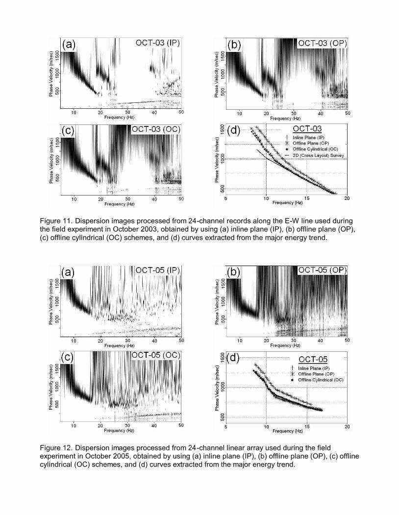
Figure 11. Dispersion images processed from 24-channel records along the E-W line used during

the field experiment in October 2003, obtained by using (a) inline plane (IP), (b) offline plane (OP),

(c) offline cylindrical (OC) schemes, and (d) curves extracted from the major energy trend.

Figure 12. Dispersion images processed from 24-channel linear array used during the field

experiment in October 2005, obtained by using (a) inline plane (IP), (b) offline plane (OP), (c) offline

cylindrical (OC) schemes, and (d) curves extracted from the major energy trend.