Embed Size (px)
Citation preview
Final Report
Long-term Wind Variability: Characteristics and Effect on
Generation
Bachelor of Science in Energy
ROBBIE PRATT

I
NAME: ROBBIE PRATT
I.D: 12140643
SUPERVISOR: DR. DAVID CORCORAN
COURSE: B.Sc. ENERGY
YEAR: FOURTH YEAR
PROJECT TITLE: LONG TERM WIND VARIABILITY:
CHARACTERISTICS AND EFFECT
ON GENERATION
DATE: 31st March 2016

II
Author’s Declaration
I hereby declare that this project is entirely my own work, in my own words, and that
all sources used in researching it are fully acknowledged and all quotations properly
identified. It has not been submitted, in whole or in part, by me or another person, for
the purpose of obtaining any other credit/grade. I understand the ethical implications
of my research, and this work meets the requirements of the Faculty of Arts,
Humanities and Social Sciences Research Ethics Committee.
Signed: ____________________ Date: ___________
III
Abstract
This paper sets out to analyse wind speeds at a number of locations in Ireland with a
view of examining the potential for wind generation in the south west of the island.
The wind index was used to provide indications of the average wind speeds at
Valentia, Shannon Airport, Birr, Dublin Airport and Malin Head. Statistical analysis
(null hypothesis) was then used to show that mean wind speed is showing a
downward trend at Valentia and Shannon Airport (both located in SW Ireland). Wind
index results from a study of UK locations (Watson et al.) were used to provide a
composite Ireland/UK correlation to produce confidence in the Irish data. The student
T-test was used to show a relationship between locations in corresponding Ireland/UK
regions with the highest confidence seen in the regions of the extreme SW of the
islands such as Valentia in Ireland.
Examination of the NAO was undertaken using the student T-test to explore if this
could be a cause of the decreasing trend at Valentia. The p-value was found to be
greater than the significance level and this indicates that there is a relationship.
The economics of wind energy production in the south west of Ireland, based on the
wind data within this paper, were looked at using the example of the 1MW turbine.
With infrastructure costs of €1.23m, 1798MWh of energy produced per annum, and
revenue of €72.167 per MWh a payback period of 9.53 years was calculated.
Weibull distribution was used for Valentia data over 20 and 50 year periods and the
distribution correlated with the experimental data within the relevant range.
IV
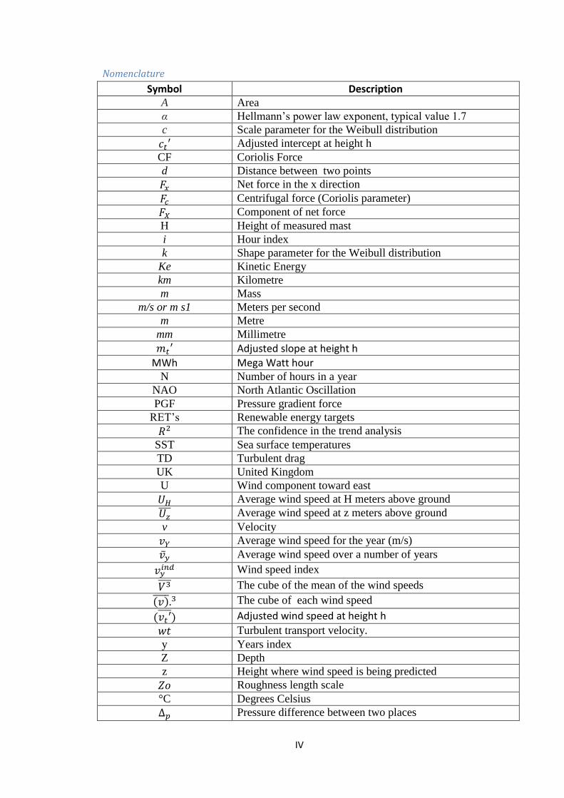
Nomenclature
Symbol Description A Area
α Hellmann’s power law exponent, typical value 1.7
c Scale parameter for the Weibull distribution
𝑐𝑡′ Adjusted intercept at height h
CF Coriolis Force
d Distance between two points
𝐹𝑥 Net force in the x direction
𝐹𝑐 Centrifugal force (Coriolis parameter)
𝐹𝑋 Component of net force
H Height of measured mast
i Hour index
k Shape parameter for the Weibull distribution
Ke Kinetic Energy
km Kilometre
m Mass
m/s or m s1 Meters per second
m Metre
mm Millimetre
𝑚𝑡′ Adjusted slope at height h
MWh Mega Watt hour N Number of hours in a year
NAO North Atlantic Oscillation
PGF Pressure gradient force
RET’s Renewable energy targets
𝑅2 The confidence in the trend analysis
SST Sea surface temperatures
TD Turbulent drag
UK United Kingdom
U Wind component toward east
𝑈𝐻 Average wind speed at H meters above ground
𝑈𝑧̅̅ ̅ Average wind speed at z meters above ground
v Velocity
𝑣𝑌 Average wind speed for the year (m/s)
�̅�𝑦 Average wind speed over a number of years
𝑣𝑦𝑖𝑛𝑑 Wind speed index
𝑉3̅̅̅̅ The cube of the mean of the wind speeds
(𝑣)̅̅ ̅̅ .3 The cube of each wind speed
(𝑣𝑡′̅̅̅̅ ) Adjusted wind speed at height h
𝑤𝑡 Turbulent transport velocity.
y Years index
Z Depth
z Height where wind speed is being predicted
𝑍𝑜 Roughness length scale
°C Degrees Celsius
Δ𝑝 Pressure difference between two places

V
~ Approximately
φ Latitude
% Percentage
≠ Not equal to.
Γ Gamma function
ρ Density
∆𝑡 Change in time
𝜏𝑝 Payback period

Table of Contents
Author’s Declaration .......................................................................................................... II
Abstract ............................................................................................................................. III
Nomenclature ................................................................................................................... IV
Chapter 1: Introduction ............................................................................................................. 1
Chapter 2: Climate of Ireland ..................................................................................................... 2
Ireland ................................................................................................................................ 2
Prevailing winds ................................................................................................................. 3
Chapter 3: Origin of the Wind ................................................................................................... 5
Advection ........................................................................................................................... 5
Pressure Gradient Force .................................................................................................... 5
Coriolis Effect ..................................................................................................................... 6
Turbulent drag force .......................................................................................................... 8
The Jet Stream ................................................................................................................... 9
The North Atlantic Oscillation ............................................................................................ 9
Cyclones ........................................................................................................................... 10
Polar front ........................................................................................................................ 11
Chapter 4: Literature Review ................................................................................................... 13
Climate Change ................................................................................................................ 13
North Atlantic Oscillation ................................................................................................. 14
Surface roughness ............................................................................................................ 14
Chapter 5: Methodology .......................................................................................................... 16
Wind index method ......................................................................................................... 16
Statistical hypothesis testing ........................................................................................... 18
Student T-test .................................................................................................................. 19

Confidence (𝑅2) ............................................................................................................... 19
Velocity scaling with height ............................................................................................. 20
Power in the wind ............................................................................................................ 21
Weibull Distribution ......................................................................................................... 22
Chapter 6: Results and Analysis (Irish Data) ............................................................................ 25
Irish Data ......................................................................................................................... 25
Payback period for a turbine at Valentia ......................................................................... 28
Comparing geographical regions in Ireland ..................................................................... 31
Chapter 7: Irish data Compared with the UK (Watson Data) .................................................. 37
Comparison with Watson ................................................................................................ 37
UK data comparison with Ireland .................................................................................... 39
Payback period for a turbine in the SW of the UK ........................................................... 42
Chapter 8: Irish data compared with the NAO ........................................................................ 45
Comparing the NAO with Wind speeds in the south west of Ireland (Valentia) ............. 45
Future predictions for the NAO ....................................................................................... 48
Chapter 9: Irish data compared with the Weibull Distribution ................................................ 49
Chapter 11: Conclusion............................................................................................................ 56
Bibliography ....................................................................................................................... a
Appendix ............................................................................................................................ A

1
Chapter 1: Introduction
With Ireland’s 2020 Renewable energy targets (RET’s) deadlines looming, the
country’s geographical location and climate means wind represents the most abundant
source of potential “non-carbon” energy production. Failure to meet the 2020 targets
would mean significant penalties being imposed by the European Commission.
This project investigates the long-term wind variability in the south west of Ireland
with a view to determining its effect on the potential of power generation by wind.
The paper will initially look at the origin of the wind and at the physical and
geographical factors that cause it to blow. By using historical data and statistical tools
such as the wind index method, valuable information on potential power generation
and associated financial returns can be produced. Data specific to Ireland will be
analysed in detail in order to produce geographically relevant results.
The primary aim of this paper is to ascertain whether the wind speed in the south west
of Ireland is reducing or increasing. The findings will serve to inform future
investment decisions in wind energy in Ireland. These decisions will influence some
of the major national strategic choices for both the energy sector and the government
in the years ahead.
2
Chapter 2: Climate of Ireland
In this chapter of the paper the climate of Ireland will be examined. This will be done
by looking at its geographic location and how this influences the climate as well as its
prevailing south westerly winds.
Ireland
Ireland is situated in the northern hemisphere in the north-western fringe of Europe at
the latitude 51-56°north and longitude 5-11°west. The North Atlantic drift has a
significant effect on the sea temperatures and hence the climate of Ireland. This
influence is greatest near the Atlantic coasts and decreases with distance travelled
inland. The main influence on the Irish climate is the Atlantic Ocean which surrounds
the island of Ireland. Due to the location, Ireland doesn’t suffer from extremes in
temperatures, precipitation or wind speeds. This cannot be said for many other
countries lying on the same latitude as Ireland. Ireland has a cool temperate oceanic
climate and its topography is varied. Hills and mountains near the coasts provide
shelter from the oceans. Summers tend to be mild and calm and winters tend to be
cold and windy.
In the extreme south-west at Valentia the mean temperature in January is 7°C and in
July the mean temperature is 15°C. Around Dublin the winter months are cooler at a
mean of 4.5°C in January and slightly warmer in summer at 15.5°C in July. The
average annual temperature in Ireland is ~9°C. In the east of the country temperatures
tend to be cooler due to the influence of the Atlantic Ocean and the prevailing winds
in the west. Nolan et al. (2011) commented on Ireland’s ideal location to exploit the
wind, with an ideal range from 6 to 8 m s-1 at 50 metres above the ground. These
wind speed values are sufficient for extracting a significant amount of power from the
wind with current wind power technology. In Ireland strong winds tend to be more
3
frequent in winter than in summer. Sunshine duration is highest in the southeast of the
country. Average rainfall varies between about 800 and 2,800mm. Rainfall figures are
highest in the northwest, west and southwest of the country, especially at the higher
altitudes. Rainfall accumulation tends to be highest in winter and lowest in early
summer.
Ireland’s climate is changing and this is true on a global level. Over the last century
there have been major changes in sea level rising and earth’s average surface area
temperature is increasing. This has major effects on the climate of Ireland. When
wind is being examined the direction and speed are the biggest factors. Globally
accurate wind speed data only goes back 10-20 years. In Ireland wind speed data has
been kept as far back as 1945. Advances in technology have improved the
measurement of wind but it is still difficult to predict long-term trends due to not
having accurate wind speed measurements in the distant past. Wind speed is measured
with a device called an anemometer which uses rotating cups. A weather vane is used
to indicate the wind direction.
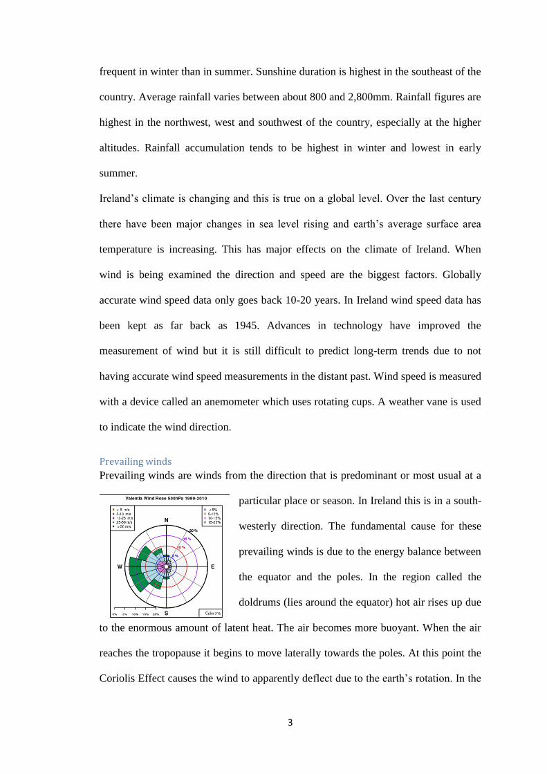
Prevailing winds
Prevailing winds are winds from the direction that is predominant or most usual at a
particular place or season. In Ireland this is in a south-
westerly direction. The fundamental cause for these
prevailing winds is due to the energy balance between
the equator and the poles. In the region called the
doldrums (lies around the equator) hot air rises up due
to the enormous amount of latent heat. The air becomes more buoyant. When the air
reaches the tropopause it begins to move laterally towards the poles. At this point the
Coriolis Effect causes the wind to apparently deflect due to the earth’s rotation. In the

4
northern hemisphere this deflection takes place to the right giving Ireland its
prevailing south-westerlies. The wind rose above shows the dominance of the wind
from the south-west at Valentia between the years 1980-2010.
In this chapter of the paper it can be seen that the predominant south westerly winds
and the Atlantic Ocean have a major effect on the climate of Ireland. In the next
chapter of this report the factors that cause the wind to blow will be examined.
5
Chapter 3: Origin of the Wind
In this chapter of the report the origin of the wind will be examined and the forces that
affect the wind will be looked at. These are advection, pressure gradient force,
Coriolis force and turbulent drag force. Also phenomena such as the jet stream, North
Atlantic Oscillation (NAO), cyclones and the polar front will be explored.
Advection
There are two types of advection: cold advection and hot advection. Cold advection is
the movement of air from a region of cold air to a region of hot air. Warm advection
is the opposite and it is the movement of warm air by the wind from a region which
has hotter air to a region which has colder air.
Pressure Gradient Force
The pressure gradient force is a force that causes the wind to blow due to difference in
pressure over a distance. The air moves from the area of higher pressure to the area of
lower pressure. A large change in pressure over a short distance is called a steep
pressure gradient and a small change in pressure over a long distance is a weak
pressure gradient.
The formula for PGF is given below:
𝑃𝐺𝐹= ΔP
𝑑 Equation 3.1
Where,
Δ𝑝 = pressure difference between two places
𝑑= distance between the two places.
The pressure gradient force is the only force that can drive the horizontal winds.
Pressure gradient force always acts at right angles to the isobars on a weather map.
6
The force exists regardless of the wind speed and is independent of wind speed. It
starts the horizontal wind, and can accelerate, decelerate or change the direction of
existing winds. The closer spaced isobars on a weather map indicate greater force.
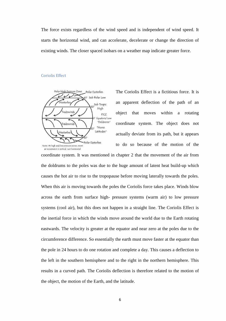
Coriolis Effect
The Coriolis Effect is a fictitious force. It is
an apparent deflection of the path of an
object that moves within a rotating
coordinate system. The object does not
actually deviate from its path, but it appears
to do so because of the motion of the
coordinate system. It was mentioned in chapter 2 that the movement of the air from
the doldrums to the poles was due to the huge amount of latent heat build-up which
causes the hot air to rise to the tropopause before moving laterally towards the poles.
When this air is moving towards the poles the Coriolis force takes place. Winds blow
across the earth from surface high- pressure systems (warm air) to low pressure
systems (cool air), but this does not happen in a straight line. The Coriolis Effect is
the inertial force in which the winds move around the world due to the Earth rotating
eastwards. The velocity is greater at the equator and near zero at the poles due to the
circumference difference. So essentially the earth must move faster at the equator than
the pole in 24 hours to do one rotation and complete a day. This causes a deflection to
the left in the southern hemisphere and to the right in the northern hemisphere. This
results in a curved path. The Coriolis deflection is therefore related to the motion of
the object, the motion of the Earth, and the latitude.

7
The Coriolis force is defined as:
𝐹𝑐 = 2𝑥Ωxsin(φ) Equation 3.2
Where,
φ = Latitude.
2𝑥Ω= 1.458x10⁻⁴𝑠1
In the Northern Hemisphere it is:
𝐹𝑦 𝐶𝐹
𝑚= 𝐹𝑐𝑣 Equation 3.3
Where,
𝐹𝑥= Net force in the x direction
𝐶𝐹= Coriolis force
𝐹𝑐= Centrifugal force (Coriolis parameter)
m = mass
v = velocity
Ireland is located in the north-hemisphere. It can be said that the Coriolis Effect has a
drastic effect on the climate and the wind direction. Coriolis force only changes the
direction of the wind. It doesn’t create the wind.

8
Turbulent drag force
Turbulent drag force is a force acting in the opposite direction to the motion of the
fluid. This slows down the wind as it goes across obstacles such as landmass. This
drag decreases with height up into the atmosphere and wind speed. The atmospheric
layer affected by friction reaches about 1000m into the air and is known as the friction
layer. Wind speeds tend to be higher above this zone.
The wind blows across the isobars towards lower pressure due to the pressure gradient
force no longer balancing the Coriolis force. The angle at which the wind blows
across the isobar is about 30 degrees. The angle at which the wind blows across the
isobar depends on the height above the ground, surface friction and the wind speed.
The turbulent drag force on a boundary layer of depth Z is:
𝐹𝑦𝑥𝑇𝐷
𝑚= −𝑤𝑡
𝑈
𝑍 Equation 3.4
Where,
𝐹𝑋 = component of net force
TD= turbulent drag
m = mass
U = wind component toward east
Z = depth
𝑤𝑡= is the turbulent transport velocity.
9
The Jet Stream
The forming of the jet stream is due to heated air from the equator rising and when
this air meets the tropopause it begins to move laterally in the direction of the Arctic.
It will move poleward and due to the spherical shape of the earth the radius decreases
due to the axis of rotation becoming closer. The change in radius means the air must
speed up. The air must move faster to the east than air which is close to the surface.
This leads to the strong south westerly winds which are very common in Ireland. The
jet stream associated with Ireland and which has a major effect on the climate is the
Polar front Jet stream. They can be up to 15km in length and a few kilometres wide.
The Jet Stream directly affects Ireland as it is located at the same latitude as Ireland.
The Irish Independent wrote “In any given year, the jet stream flows generally
between the latitudes of 40 degrees north and 70 degrees north.” In January and
February 2014 it was located just over the south of Ireland and so Ireland, especially
the south and south west, “was battered by its eighth storm in a little over 10 weeks
yesterday” (The Independent 13/02/2014)
The North Atlantic Oscillation
The North Atlantic Oscillation is a reversal of pressure over the Atlantic. It has an
effect on the climate of Northern Europe, hence, Ireland. It is caused by the change in
pressure between the Icelandic low and the Azores high. There are two phases to the
NAO, the positive phase and the negative phase. For the positive phase the pressure at
the pole drops and the pressure at the Azores rises causing a huge pressure difference
between the regions and this strengthens the westerlies. These stronger winds cause
strong cyclones which move over northern Europe. For the negative phase the
pressure at the pole rises and pressure drops at the Azores. This change is pressure

10
weakens the westerlies and fewer storms move across the Atlantic. Due to this winters
tend to be cold and dry in northern Europe. The NAO is not periodical and hence it
doesn’t have to stay in one phase for a prolonged time. It also varies from year to
year. It can stay in one phase for several years. Over the last 30 years the NAO has
been more in the positive phase than the negative.
In the winter of 2009/10 the NAO was strongly negative over Ireland and Ireland had
a very cold winter and the average wind speed for the year was at an all-time low
across the country.
Cyclones
A cyclone is an area of closed, circular fluid motion rotating in the same direction as
the Earth. The lows are centres of low pressure and form in the middle latitudes. This
is usually characterized by inward spiralling winds that rotate counter clockwise in the
Northern Hemisphere and clockwise in the Southern Hemisphere of the Earth due to
the Coriolis Effect. The effects of cyclones (low in pressure) in Europe include strong
winds and heavy rainfall. The highs are centres of high pressure and are called
anticyclones. “Ireland’s climate is heavily influenced by the North Atlantic Ocean. As
sea surface temperatures (SST) are projected to rise due to global warming the impact
on cyclone activity is investigated using two pairs of climate simulations performed
with the Rossby Centre regional climate model RCA3. The results show an increase
in the frequency of the very intense cyclones with maximum wind speeds of more
than 30 m/s, and also increases in the extreme values of wind and (around Ireland)
precipitation associated with the cyclones. This will translate into an increased risk of
storm damage and flooding, with elevated storm surges along Irish coasts.”
(http://www.met.ie/publications/irelandinawarmerworld.pdf)
11
Polar front
The polar front is a front in the northern hemisphere which affects the climate of
Ireland. The polar front is a zone of transition between warm air from the tropics
which is moving northwards and air moving southwards which is colder, drier and
denser from the pole. The polar front is one of the main factors which influence the
weather Ireland gets on a day in, day out basis. As the mild weather that crosses
Ireland from a South-westerly direction continues northwards, it encounters cold air
which is moving from the north. These two masses of air travelling in different
directions do not mix. They are then separated by a boundary layer called the polar
front which is a zone of low pressure. In these zones of low pressure, Ireland gets
cloudy, humid weather with rain, followed by brighter, colder weather. This is typical
of the Irish climate. Ireland's climate is varied and Ireland experiences a range of air
masses but air masses of polar origin are the most common and have a very long track
over the Atlantic Ocean. Even winds in the south-westerly direction can give Ireland
polar air. Air direction from the middle latitudes and from the north are uncommon
which means Irelands weather is varied but it doesn’t range drastically.
Warm fronts are followed by a cold front and the cold front catches up with the warm
front and an occluded front forms. When this occurs, the warm air is separated
(occluded) from the cyclone.
"In general the Atlantic low-pressure systems are well established by December, and
depressions move rapidly eastward in December and January, bringing strong winds
with appreciable frontal rainfall to Ireland. Occasionally the cold anticyclone over
Europe extends its influence westwards to Ireland, giving dry cold periods lasting
several days."

12
Ireland’s climate is dynamic. Its location makes it an ideal candidate for wind energy.
To understand the wind variability in Ireland we must go further afield and look at the
global wind patterns and effects such as the Coriolis Effect (which gives a better
understanding of the wind patterns in northern Europe), the prevailing winds and why
these winds move through space in the way they do. Power from the wind varies on
all time-scales, seconds, months, decades etc. In this study we are going to look at the
long term trends over northern Europe, Ireland and more precisely the south west of
Ireland.
13
Chapter 4: Literature Review
Watson et al. (2015) mentioned that knowledge of wind speed variability is important
for wind farm developers and operators so that there is a minimum long term risk of
fluctuation to wind speeds and revenue. During the last decades the general trend in
the northern hemisphere’s wind speed is a decreasing one Widén et al. (2015). The
reasons for this are not fully clear but there are some theories of why it is happening.
Climate Change
Nolan et al. (2011) suggests climate change may be a factor to consider in the
variability of wind speed in the future of Ireland. Future predictions show 4 to 10%
more energy available in the wind during winter and 5 to 14% less during summer
months at 60m above sea level and this represents an overall drop in wind speed over
the island of Ireland if we look at it annually. (But this could also be due to the North
Atlantic Oscillation phase shift.) The figures were calculated using the Kolmogorov-
Smirnov test using past wind speed data. A possible reason for the unevenly
distributed wind speed may be due to an increase in cyclone activity. Intense cyclones
developing in the North Atlantic Ocean are thought to increase in the winter months
and to decrease in the summer months. The future wind speed predictions correlate
with the cyclone activity. A cause for these cyclones which have increased intensity
could be an increase in moisture supply due to increasing sea water temperatures and
the increase in latent heat flux would mean an increase in the intensity of cyclones.
Watson et al. (2015) uses the wind speed index method and reviews a period of 18
years from 1983-2011 in the UK looking at 6 different stations located across the
country. From his finding, a decrease in wind speed is seen in five of the six stations.
14
Like Nolan et al. Watson found that the largest decrease in wind speeds occurred in
the winter months and smallest in the summer months. When looking at the wind
speed data we must take into account that the instrument measurement may be a
factor due to there being significant changes in the height that measurements were
taken at the different stations. The correlation of the wind speeds to 10m above the
ground is a factor to take into consideration when looking at the results.
North Atlantic Oscillation
Earl et al. believes there is a significant correlation between variability in the wind
speed fluctuation and the North Atlantic Oscillation (NAO). He looked at the south
westerly winds in the UK for the year 1986 and saw that there was a correlation
between the wind speeds of certain months when the strong positive NAO was
present over the Atlantic Ocean. This holds true the possibility that the NAO is
positively correlated with the variability in the wind. A more recent observation
would be the winter of 2009/10 which had a very negative NAO and because of this
extremely low wind speeds for those months were observed in Ireland and the UK. In
the UK when the NAO is in its positive state winds are strong and predominantly in
the south west direction and in periods when the NAO is in a strong negative trend the
speeds are reduced and wind direction is very much varied and predominantly from
the north east (Earl et al).
Surface roughness
Vautard et al. (2010) found a correlation between increased surface roughness and
decrease in wind speed at a height of 10m from the ground between the years 1979-
2008 in the Netherlands. Wever (2011) also observed the surface roughness in the
15
Netherlands and looked at the impact of increased urbanisation, forest area, increase
in agriculture and tall crops such as corn. He recorded a yearly decrease in annual
mean wind speeds of 3.1 percent between 1981 and 2009.
Bakker et al. (2010) suggests that the climate has always been subject to change. The
climate of northwest Europe has not structurally changed over the previous 100/200
years. Between the 1960s and the mid-1990s Europe saw a large increase in wind
speeds and these trends have always happened. There are fluctuations but this applies
to climates all over the world. Bakker mentions the Hurst phenomenon and how
similar events such as drought or extremes in temperatures seem to occur in patterns
and cycles.
There is evidence to support that wind speeds in the north west of Europe are
decreasing. Why this is happening is not certain. There are many different thoughts on
what is setting this downward trend, especially over the last 20 years - surface
roughness, North Atlantic Oscillation and climate change to list a few. Wind data has
been analysed using different methods such as wind index, Hurst phenomenon etc. In
this paper the wind index method will be used as a means of analysing wind data and
providing an indication of the mean wind speed. Wind data on an annual basis will be
used following the same method used by Watson et al. (2015)
16
Chapter 5: Methodology
The wind data used in this report will be sourced from Met Éireann weather stations
across the country. (Alternative data will be used when looking further afield in the
UK and Northern Europe) The wind data from Met Éireann is divided into intervals of
1 hour averages. This chapter will show how the data will be analysed. The Methods
that will be used are the wind indices method and statistical hypotheses testing. Other
methods such as the Weibull distribution method will be looked at, at a later period
following completion of this paper.
Wind index method
A wind index provides an indication of the average (mean) wind speed. It is a
statistical tool that can be used to look at the long-term wind speed trend of a region.
This is usually done using regular intervals to perform the analysis on a monthly or
yearly timescale. The wind index is used as a reference wind speed when looking at
long term production Atkinson et al. (2005).
The wind speed index can also be used to provide a financial estimate of the return on
a wind farm. An increase or decrease in power available in the wind will have a major
effect on power production. The trends in the wind are very important due to wind
farms having life spans of up to 40/50 years and climates can significantly change
over a much shorter period. Estimating the energy production of the wind farm in the
future is possible when analysis of the past trends has been done. Watson et al.
(2013).

17
To calculate the wind speed index ideally wind speed data which is taken hourly for a
few years will be used in the calculation. Firstly the mean wind speed for each year
must be found by using the following equation:
𝑣𝑦 = 1
𝑁∑ 𝑣𝑖𝑦
𝑁
𝑖=𝑗 Equation 5.1
Where,
N= the number of hours in a year (hr)
𝑣𝑌= the average wind speed for the year (m/s)
i= is the hour index
y= is the year index
Next the average of all the years in the index must be calculated using the following
equation.
�̅�𝑦= 1
𝑁∑ 𝑣𝑦
𝑥 𝑒𝑛𝑑
𝑥 𝑠𝑡𝑎𝑟𝑡 Equation 5.2
Where,
�̅�𝑦=is the average wind speed over 𝑁𝑦 years

18
Finally the average wind speed of each year is divided by the average of all the years
in the period to get the wind index value. Formula is below:
𝑣𝑦𝑖𝑛𝑑𝑒𝑥 =
𝑣𝑦
�̅�𝑦 Equation 5.3
Where,
𝑣𝑦𝑖𝑛𝑑= the wind speed index
The aim of this paper is to look at the variability of wind speed in the south west of
Ireland. The wind index will be used to analyse data both at a national level and a
regional level and will be used to compare with indices from other locations in the
North West of Europe.
Statistical hypothesis testing
A statistical hypothesis test is a method in statistics which allows the analysis of
underlying distribution by analysing data. Two statistical data sets will be compared.
In each case a hypothesis is proposed for the statistical relationship between the two
data sets. The comparison is said to be significant if the relationship between the two
data sets would be an unlikely outcome of the null hypothesis. Hypothesis tests are
used in determining what outcomes of a study would lead to a rejection of the null
hypothesis.
To be able to reject a hypothesis the p-value must be looked at. The p-value is given
as the probability of receiving a result equal to or greater than what was actually
viewed. Before the test is performed, a threshold value is chosen. This is the

19
significance level of the test and this will be 0.05 for this paper and given the symbol
α (alpha).
If the p-value is less than the required significance level, then we say the null
hypothesis is rejected at the given level of significance. Rejection of the null
hypothesis is a conclusion.
If the p-value is not less than the required significance level then the test has no result.
The evidence is insufficient to support a conclusion.
Student T-test
This statistical method is used to see if two samples of data are significantly different
from each other. Like the hypothesis testing, the student t-test relies on the p-value
and a significance level which it must achieve or not achieve to be rejected or
accepted. The hypothesis states that both slopes are not equal. If the p-value is less
than the significance level, then the null hypothesis is rejected. This means the slopes
are deemed to be similar. If the p-value is greater than the significance level, then the
null hypothesis is accepted. This means are not similar.
Confidence (R^2)
The confidence interval describes the certainty associated with the statistical method
used. The value of R falls between 0 and 1. A value nearer to 1 means it can be said
that the sampling method used is of a high confidence. If the value falls towards 0 it
can be said that the sampling method used is of a low confidence.

20
Velocity scaling with height
In this project, Hellmann’s Power Law will be as a way of scaling height from the met
mast to the height of the turbine. This in turn will give the wind speed at the given
height of the tower and from this we can calculate the power in the wind at that
height. The following formula is used for this calculation:
• Hellmann’s Power Law:
𝑈𝑧̅̅̅̅
𝑈𝐻= (
𝑧
𝐻) .∝ Equation 5.4
• 𝑧 – Height where wind speed is being predicted
• 𝐻 – Height of measurement mast
• 𝑈𝑧̅̅ ̅– Average wind speed at z meters above ground
• 𝑈𝐻 – Average wind speed at H meters above ground
• 𝛼 – Hellmann’s power law exponent, typical value 1.7
Another way to scale the wind speed at different heights is by using the velocity
scaling with height method which uses logs. The Equation is as follows:
𝑈𝑧
𝑈𝐻 =
𝑙𝑛(𝑍
𝑍𝑜)
𝑙𝑛(𝐻
𝑍𝑜) Equation 5.5
Where,
�̅�𝑧= Average wind speed at Z meters above ground
�̅�𝐻= Average wind speed at H meters above ground
𝑍= Height where wind speed is being predicted
21
𝑍𝑜= Roughness length scale
𝐻= Height of measure mast
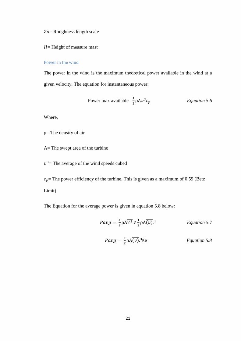
Power in the wind
The power in the wind is the maximum theoretical power available in the wind at a
given velocity. The equation for instantaneous power:
Power max available= 1
2ρA𝑣3𝑐𝑝 Equation 5.6
Where,
ρ= The density of air
A= The swept area of the turbine
𝑣3= The average of the wind speeds cubed
𝑐𝑝= The power efficiency of the turbine. This is given as a maximum of 0.59 (Betz
Limit)
The Equation for the average power is given in equation 5.8 below:
𝑃𝑎𝑣𝑔 = 1
2ρA𝑉3̅̅̅̅ ≠
1
2ρA(𝑣)̅̅ ̅̅ .3 Equation 5.7
𝑃𝑎𝑣𝑔 = 1
2ρA(𝑣)̅̅ ̅̅ .3Ke Equation 5.8
22
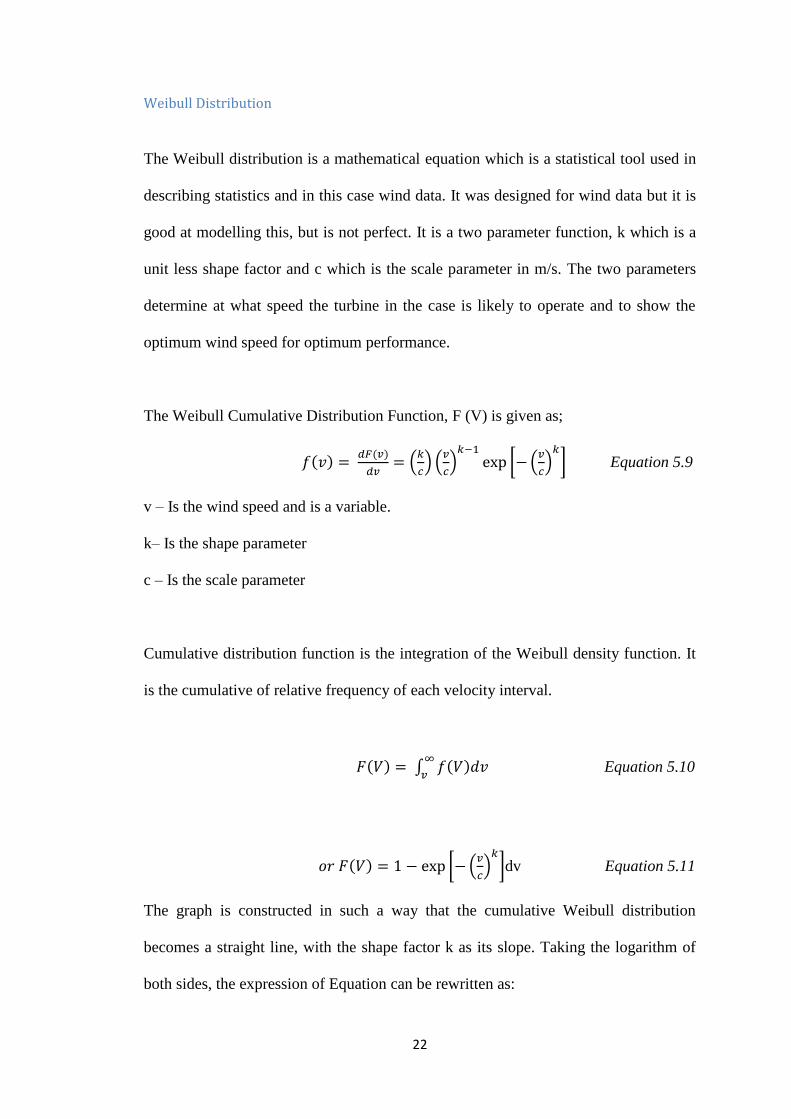
Weibull Distribution
The Weibull distribution is a mathematical equation which is a statistical tool used in
describing statistics and in this case wind data. It was designed for wind data but it is
good at modelling this, but is not perfect. It is a two parameter function, k which is a
unit less shape factor and c which is the scale parameter in m/s. The two parameters
determine at what speed the turbine in the case is likely to operate and to show the
optimum wind speed for optimum performance.
The Weibull Cumulative Distribution Function, F (V) is given as;
𝑓(𝑣) = 𝑑𝐹(𝑣)
𝑑𝑣= (
𝑘
𝑐) (
𝑣
𝑐)
𝑘−1
exp [− (𝑣
𝑐)
𝑘
] Equation 5.9
v – Is the wind speed and is a variable.
k– Is the shape parameter
c – Is the scale parameter
Cumulative distribution function is the integration of the Weibull density function. It
is the cumulative of relative frequency of each velocity interval.
𝐹(𝑉) = ∫ 𝑓(𝑉)𝑑𝑣∞
𝑣 Equation 5.10
𝑜𝑟 𝐹(𝑉) = 1 − exp [− (𝑣
𝑐)
𝑘
]dv Equation 5.11
The graph is constructed in such a way that the cumulative Weibull distribution
becomes a straight line, with the shape factor k as its slope. Taking the logarithm of
both sides, the expression of Equation can be rewritten as:
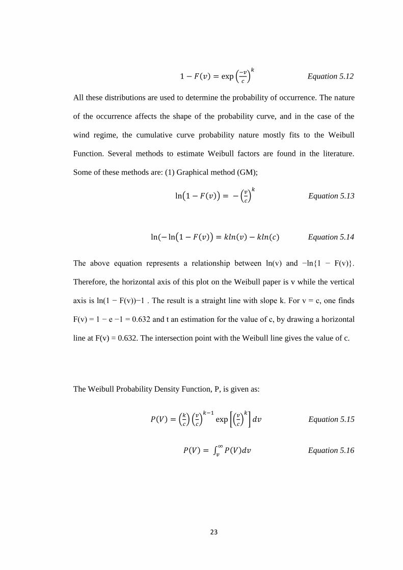
23
1 − 𝐹(𝑣) = exp (−𝑣
𝑐)
𝑘
Equation 5.12
All these distributions are used to determine the probability of occurrence. The nature
of the occurrence affects the shape of the probability curve, and in the case of the
wind regime, the cumulative curve probability nature mostly fits to the Weibull
Function. Several methods to estimate Weibull factors are found in the literature.
Some of these methods are: (1) Graphical method (GM);
ln(1 − 𝐹(𝑣)) = − (𝑣
𝑐)
𝑘
Equation 5.13
ln (− ln(1 − 𝐹(𝑣)) = 𝑘𝑙𝑛(𝑣) − 𝑘𝑙𝑛(𝑐) Equation 5.14
The above equation represents a relationship between ln(v) and −ln{1 − F(v)}.
Therefore, the horizontal axis of this plot on the Weibull paper is v while the vertical
axis is ln(1 − F(v))−1 . The result is a straight line with slope k. For v = c, one finds
F(v) = 1 − e −1 = 0.632 and t an estimation for the value of c, by drawing a horizontal
line at F(v) = 0.632. The intersection point with the Weibull line gives the value of c.
The Weibull Probability Density Function, P, is given as:
𝑃(𝑉) = (𝑘
𝑐) (
𝑣
𝑐)
𝑘−1
exp [(𝑣
𝑐)
𝑘
] 𝑑𝑣 Equation 5.15
𝑃(𝑉) = ∫ 𝑃(𝑉)𝑑𝑣∞
𝑣 Equation 5.16
24
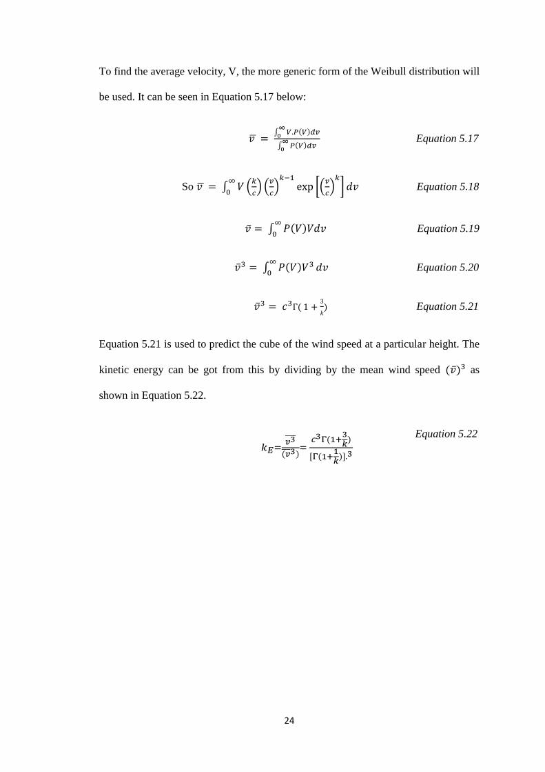
To find the average velocity, V, the more generic form of the Weibull distribution will
be used. It can be seen in Equation 5.17 below:
𝑣 ̅ = ∫ 𝑉.𝑃(𝑉)𝑑𝑣
∞0
∫ 𝑃(𝑉)𝑑𝑣∞
0
Equation 5.17
So 𝑣 ̅ = ∫ 𝑉 (𝑘
𝑐) (
𝑣
𝑐)
𝑘−1
exp [(𝑣
𝑐)
𝑘
] 𝑑𝑣∞
0 Equation 5.18
�̅� = ∫ 𝑃(𝑉)𝑉𝑑𝑣∞
0 Equation 5.19
�̅�3 = ∫ 𝑃(𝑉)𝑉3∞
0𝑑𝑣 Equation 5.20
�̅�3 = 𝑐3Γ( 1 +3
𝑘) Equation 5.21
Equation 5.21 is used to predict the cube of the wind speed at a particular height. The
kinetic energy can be got from this by dividing by the mean wind speed (�̅�)3 as
shown in Equation 5.22.
𝑘𝐸=𝑣3̅̅̅̅
(𝑣̅̅ ̅3)=
𝑐3Γ(1+3𝑘
)
[Γ(1+1𝑘
)].3
Equation 5.22
25
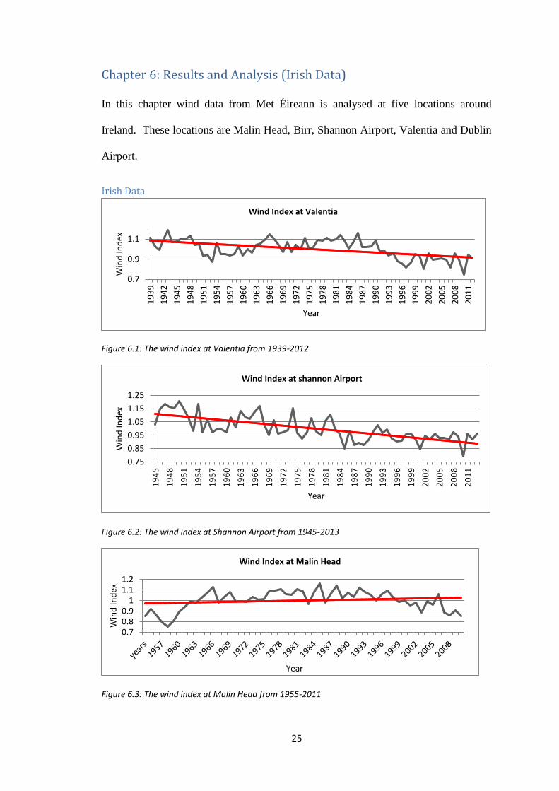
Chapter 6: Results and Analysis (Irish Data)
In this chapter wind data from Met Éireann is analysed at five locations around
Ireland. These locations are Malin Head, Birr, Shannon Airport, Valentia and Dublin
Airport.
Irish Data
Figure 6.1: The wind index at Valentia from 1939-2012
Figure 6.2: The wind index at Shannon Airport from 1945-2013
Figure 6.3: The wind index at Malin Head from 1955-2011
0.7
0.9
1.1
19
39
19
42
19
45
19
48
19
51
19
54
19
57
19
60
19
63
19
66
19
69
19
72
19
75
19
78
19
81
19
84
19
87
19
90
19
93
19
96
19
99
20
02
20
05
20
08
20
11
Win
d In
dex
Year
Wind Index at Valentia
0.75
0.85
0.95
1.05
1.15
1.25
19
45
19
48
19
51
19
54
19
57
19
60
19
63
19
66
19
69
19
72
19
75
19
78
19
81
19
84
19
87
19
90
19
93
19
96
19
99
20
02
20
05
20
08
20
11
Win
d In
dex
Year
Wind Index at shannon Airport
0.70.80.9
11.11.2
Win
d In
dex
Year
Wind Index at Malin Head
26
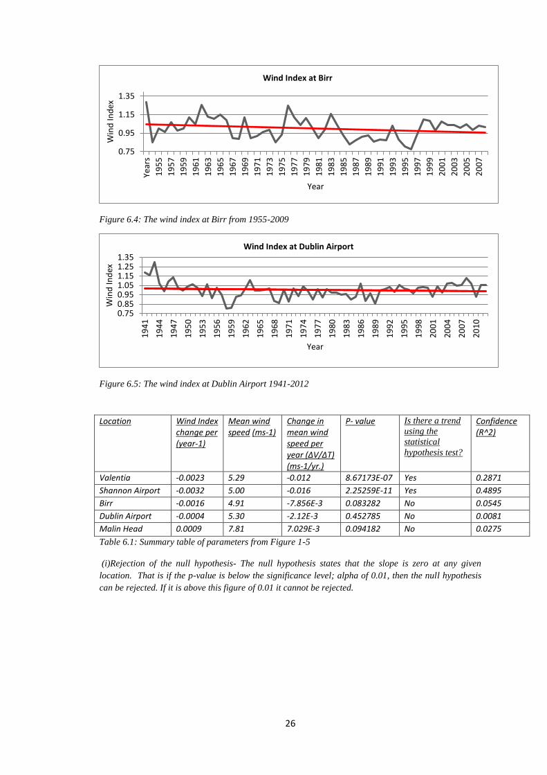
Figure 6.4: The wind index at Birr from 1955-2009
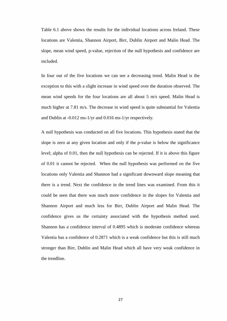
Figure 6.5: The wind index at Dublin Airport 1941-2012
Table 6.1: Summary table of parameters from Figure 1-5
(i)Rejection of the null hypothesis- The null hypothesis states that the slope is zero at any given
location. That is if the p-value is below the significance level; alpha of 0.01, then the null hypothesis
can be rejected. If it is above this figure of 0.01 it cannot be rejected.
0.75
0.95
1.15
1.35
Year
s
19
55
19
57
19
59
19
61
19
63
19
65
19
67
19
69
19
71
19
73
19
75
19
77
19
79
19
81
19
83
19
85
19
87
19
89
19
91
19
93
19
95
19
97
19
99
20
01
20
03
20
05
20
07
Win
d In
dex
Year
Wind Index at Birr
0.750.850.951.051.151.251.35
19
41
19
44
19
47
19
50
19
53
19
56
19
59
19
62
19
65
19
68
19
71
19
74
19
77
19
80
19
83
19
86
19
89
19
92
19
95
19
98
20
01
20
04
20
07
20
10
Win
d In
dex
Year
Wind Index at Dublin Airport
Location Wind Index change per (year-1)
Mean wind speed (ms-1)
Change in mean wind speed per year (ΔV/ΔT) (ms-1/yr.)
P- value Is there a trend
using the
statistical
hypothesis test?
Confidence (R^2)
Valentia -0.0023 5.29 -0.012 8.67173E-07 Yes 0.2871
Shannon Airport -0.0032 5.00 -0.016 2.25259E-11 Yes 0.4895
Birr -0.0016 4.91 -7.856E-3 0.083282 No 0.0545
Dublin Airport -0.0004 5.30 -2.12E-3 0.452785 No 0.0081
Malin Head 0.0009 7.81 7.029E-3 0.094182 No 0.0275
27
Table 6.1 above shows the results for the individual locations across Ireland. These
locations are Valentia, Shannon Airport, Birr, Dublin Airport and Malin Head. The
slope, mean wind speed, p-value, rejection of the null hypothesis and confidence are
included.
In four out of the five locations we can see a decreasing trend. Malin Head is the
exception to this with a slight increase in wind speed over the duration observed. The
mean wind speeds for the four locations are all about 5 m/s speed. Malin Head is
much higher at 7.81 m/s. The decrease in wind speed is quite substantial for Valentia
and Dublin at -0.012 ms-1/yr and 0.016 ms-1/yr respectively.
A null hypothesis was conducted on all five locations. This hypothesis stated that the
slope is zero at any given location and only if the p-value is below the significance
level; alpha of 0.01, then the null hypothesis can be rejected. If it is above this figure
of 0.01 it cannot be rejected. When the null hypothesis was performed on the five
locations only Valentia and Shannon had a significant downward slope meaning that
there is a trend. Next the confidence in the trend lines was examined. From this it
could be seen that there was much more confidence in the slopes for Valentia and
Shannon Airport and much less for Birr, Dublin Airport and Malin Head. The
confidence gives us the certainty associated with the hypothesis method used.
Shannon has a confidence interval of 0.4895 which is moderate confidence whereas
Valentia has a confidence of 0.2871 which is a weak confidence but this is still much
stronger than Birr, Dublin and Malin Head which all have very weak confidence in
the trendline.
28
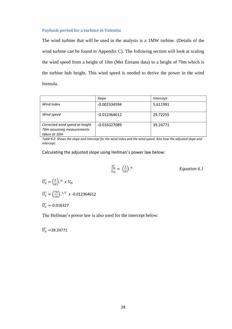
Payback period for a turbine at Valentia
The wind turbine that will be used in the analysis is a 1MW turbine. (Details of the
wind turbine can be found in Appendix C). The following section will look at scaling
the wind speed from a height of 10m (Met Éireann data) to a height of 70m which is
the turbine hub height. This wind speed is needed to derive the power in the wind
formula.
Slope Intercept
Wind Index -0.002334594 5.611991
Wind speed -0.012364612
29.72255
Corrected wind speed at height 70m assuming measurements taken at 10m
-0.016327089
39.24771
Table 6.2: Shows the slope and intercept for the wind index and the wind speed. Also how the adjusted slope and intercept.
Calculating the adjusted slope using Hellman’s power law below:
𝑈𝑧̅̅̅̅
𝑈𝐻= (
𝑧
𝐻) .∝ Equation 6.1
𝑈𝑧̅̅ ̅ = (
𝑧
𝐻) .∝ 𝑥 𝑈𝐻
𝑈𝑧̅̅ ̅ = (
70
10) .1/7 𝑥 -0.012364612
𝑈𝑧̅̅ ̅ =-0.016327
The Hellman’s power law is also used for the intercept below:
𝑈𝑧̅̅ ̅ =39.24771
29
Next the mean cubed wind speed must be extrapolated using the following formula
the average mean wind speed to be cubed. (Derivation for (𝑣𝑡′̅̅̅̅ )3 is in Appendix F):
(𝑣𝑡′̅̅̅̅ )3 = 1
4𝑚𝑡′∆𝑡 (𝑚𝑡′𝑡𝑒𝑛𝑑 + 𝑐𝑡′)4- (𝑚𝑡′𝑡𝑠𝑡𝑎𝑟𝑡 + 𝑐𝑡′)4 Equation 6.2
(𝑣𝑡′̅̅̅̅ )3 = 1
4(−0.016327)(17) [(−0.016327)(2030)(39.24771]- [(−0.016327)(2013)(39.24771)]4
(𝑣𝑡′̅̅̅̅ )3 = 243.4
Now that (𝑣𝑡′̅̅̅̅ )3 has been calculated the max power for the 1 MW turbine can be
found. The Betz limit will be multiplied by the power in the wind equation below to
give the maximum theoretical power generated by the turbine. This formula is as
follows:
Power max available= 1
2ρA𝑣3𝐵𝑒𝑡𝑧 𝐿𝑖𝑚𝑖𝑡 Equation
6.3
Power = 1
2(1.225)(π[27.2]^2)(243.4)(0.59) = 204272W or 0.204MWh
Now that the maximum theoretical power for the 1MWh turbine has been calculated it
is possible to find the energy generated for the year. This is done by the following
formula:
𝑃𝑜𝑤𝑒𝑟̅̅ ̅̅ ̅̅ ̅̅ ̅ 𝑥 𝛥𝑡 = 𝑒𝑛𝑒𝑟𝑔𝑦̅̅ ̅̅ ̅̅ ̅̅ ̅̅ Equation 6.4
204272W 𝑥 365 𝑥 24 = 1789𝑀𝑊ℎ/𝑦𝑟
This can be divided by the average cost for one MWh of electricity which was found
to be €72.167 for the year 2015. This figure will be used to the following calculation.
(Please find details in Appendix A).
30
𝑒𝑛𝑒𝑟𝑔𝑦̅̅ ̅̅ ̅̅ ̅̅ ̅̅ 𝑥 𝑝𝑟𝑖𝑐𝑒 𝑝𝑒𝑟 𝑀𝑊ℎ = 𝑅𝑒𝑣𝑒𝑛𝑢𝑒 𝑓𝑜𝑟 𝑡ℎ𝑒 𝑦𝑒𝑎𝑟 Equation 6.5
1789MWh x €72.167= €129107
The cost of construction of a 1MW turbine is in the vicinity of €1,230,000. This
includes an operational and maintenance cost of 1-2 percent a year for 10 years. The
construction cost/operation/maintenance cost is now divided by the revenue for the
year to give the payback period in years as follows.
€1,230,000/ €129,107 = 9.53 years
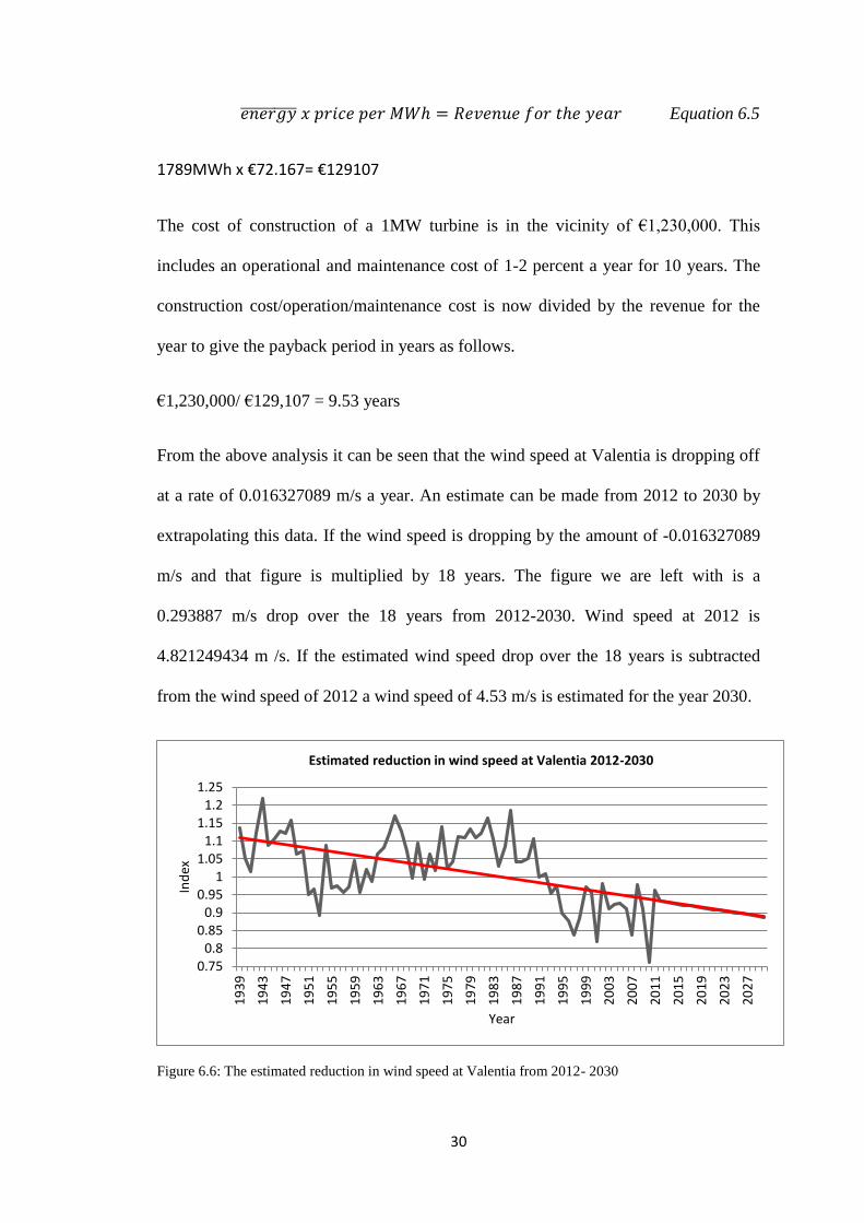
From the above analysis it can be seen that the wind speed at Valentia is dropping off
at a rate of 0.016327089 m/s a year. An estimate can be made from 2012 to 2030 by
extrapolating this data. If the wind speed is dropping by the amount of -0.016327089
m/s and that figure is multiplied by 18 years. The figure we are left with is a
0.293887 m/s drop over the 18 years from 2012-2030. Wind speed at 2012 is
4.821249434 m /s. If the estimated wind speed drop over the 18 years is subtracted
from the wind speed of 2012 a wind speed of 4.53 m/s is estimated for the year 2030.
Figure 6.6: The estimated reduction in wind speed at Valentia from 2012- 2030
0.750.8
0.850.9
0.951
1.051.1
1.151.2
1.25
19
39
19
43
19
47
19
51
19
55
19
59
19
63
19
67
19
71
19
75
19
79
19
83
19
87
19
91
19
95
19
99
20
03
20
07
20
11
20
15
20
19
20
23
20
27
Ind
ex
Year
Estimated reduction in wind speed at Valentia 2012-2030
31
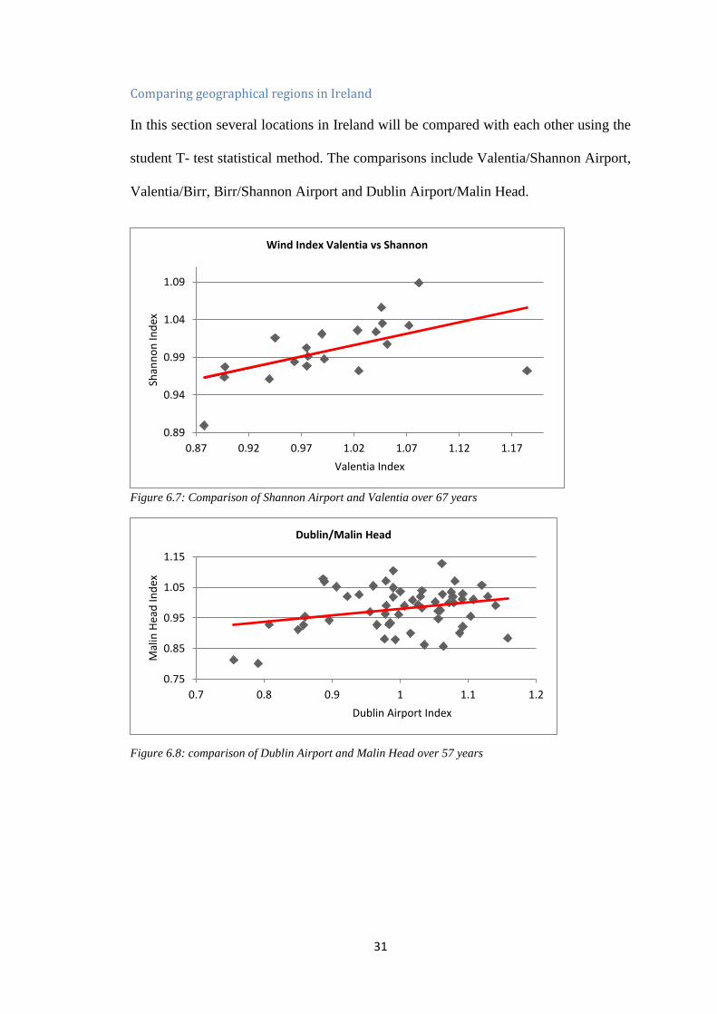
Comparing geographical regions in Ireland
In this section several locations in Ireland will be compared with each other using the
student T- test statistical method. The comparisons include Valentia/Shannon Airport,
Valentia/Birr, Birr/Shannon Airport and Dublin Airport/Malin Head.
Figure 6.7: Comparison of Shannon Airport and Valentia over 67 years
Figure 6.8: comparison of Dublin Airport and Malin Head over 57 years
0.89
0.94
0.99
1.04
1.09
0.87 0.92 0.97 1.02 1.07 1.12 1.17
Shan
no
n In
dex
Valentia Index
Wind Index Valentia vs Shannon
0.75
0.85
0.95
1.05
1.15
0.7 0.8 0.9 1 1.1 1.2
Mal
in H
ead
Ind
ex
Dublin Airport Index
Dublin/Malin Head
32
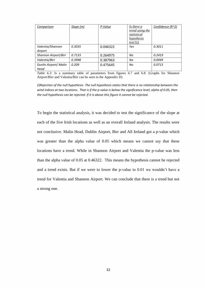
Comparison Slope (m) P-Value Is there a
trend using the
statistical
hypothesis
test?(i)
Confidence (R^2)
Valentia/Shannon Airport
0.3035 0.046322 Yes 0.3011
Shannon Airport/Birr 0.7133 0.264975 No 0.2419
Valentia/Birr 0.3998 0.387963 No 0.0949
Dunlin Airport/ Malin Head
0.209 0.475645 No 0.0713
Table 6.3: Is a summary table of parameters from figures 6.7 and 6.8. (Graphs for Shannon
Airport/Birr and Valentia/Birr can be seen in the Appendix D)
(i)Rejection of the null hypothesis- The null hypothesis states that there is no relationship between the
wind indices at two locations. That is if the p-value is below the significance level; alpha of 0.05, then
the null hypothesis can be rejected. If it is above this figure it cannot be rejected.
To begin the statistical analysis, it was decided to test the significance of the slope at
each of the five Irish locations as well as an overall Ireland analysis. The results were
not conclusive. Malin Head, Dublin Airport, Birr and All Ireland got a p-value which
was greater than the alpha value of 0.05 which means we cannot say that these
locations have a trend. While in Shannon Airport and Valentia the p-value was less
than the alpha value of 0.05 at 0.46322. This means the hypothesis cannot be rejected
and a trend exists. But if we were to lower the p-value to 0.01 we wouldn’t have a
trend for Valentia and Shannon Airport. We can conclude that there is a trend but not
a strong one.
33
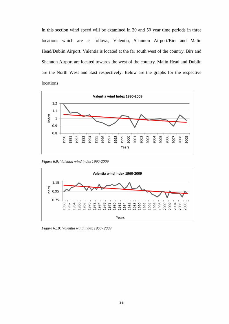
In this section wind speed will be examined in 20 and 50 year time periods in three
locations which are as follows, Valentia, Shannon Airport/Birr and Malin
Head/Dublin Airport. Valentia is located at the far south west of the country. Birr and
Shannon Airport are located towards the west of the country. Malin Head and Dublin
are the North West and East respectively. Below are the graphs for the respective
locations
Figure 6.9: Valentia wind index 1990-2009
Figure 6.10: Valentia wind index 1960- 2009
0.8
0.9
1
1.1
1.2
19
90
19
91
19
92
19
93
19
94
19
95
19
96
19
97
19
98
19
99
20
00
20
01
20
02
20
03
20
04
20
05
20
06
20
07
20
08
20
09
Ind
ex
Years
Valentia wind Index 1990-2009
0.75
0.95
1.15
19
60
19
62
19
64
19
66
19
68
19
70
19
72
19
74
19
76
19
78
19
80
19
82
19
84
19
86
19
88
19
90
19
92
19
94
19
96
19
98
20
00
20
02
20
04
20
06
20
08
Ind
ex
Years
Valentia wind index 1960-2009
34
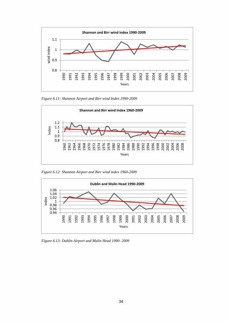
Figure 6.11: Shannon Airport and Birr wind Index 1990-2009
Figure 6.12: Shannon Airport and Birr wind index 1960-2009
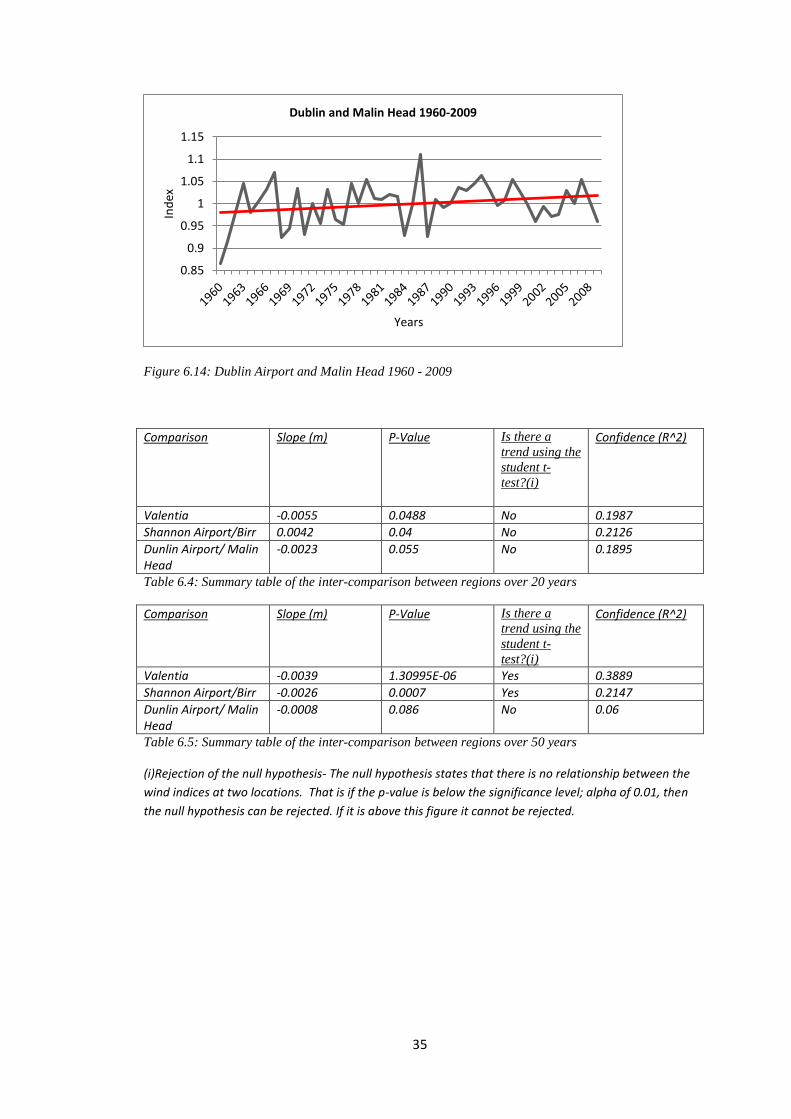
Figure 6.13: Dublin Airport and Malin Head 1990- 2009
0.8
0.9
1
1.1
19
90
19
91
19
92
19
93
19
94
19
95
19
96
19
97
19
98
19
99
20
00
20
01
20
02
20
03
20
04
20
05
20
06
20
07
20
08
20
09
win
d in
dex
Years
Shannon and Birr wind Index 1990-2009
0.80.9
11.11.2
19
60
19
62
19
64
19
66
19
68
19
70
19
72
19
74
19
76
19
78
19
80
19
82
19
84
19
86
19
88
19
90
19
92
19
94
19
96
19
98
20
00
20
02
20
04
20
06
20
08
Ind
ex
Years
Shannon and Birr wind Index 1960-2009
0.940.960.98
11.021.041.06
19
90
19
91
19
92
19
93
19
94
19
95
19
96
19
97
19
98
19
99
20
00
20
01
20
02
20
03
20
04
20
05
20
06
20
07
20
08
20
09
Ind
ex
Years
Dublin and Malin Head 1990-2009
35
Figure 6.14: Dublin Airport and Malin Head 1960 - 2009
Comparison Slope (m) P-Value Is there a
trend using the
student t-
test?(i)
Confidence (R^2)
Valentia -0.0055 0.0488 No 0.1987
Shannon Airport/Birr 0.0042 0.04 No 0.2126
Dunlin Airport/ Malin Head
-0.0023 0.055 No 0.1895
Table 6.4: Summary table of the inter-comparison between regions over 20 years
Comparison Slope (m) P-Value Is there a
trend using the
student t-
test?(i)
Confidence (R^2)
Valentia -0.0039 1.30995E-06 Yes 0.3889
Shannon Airport/Birr -0.0026 0.0007 Yes 0.2147
Dunlin Airport/ Malin Head
-0.0008 0.086 No 0.06
Table 6.5: Summary table of the inter-comparison between regions over 50 years
(i)Rejection of the null hypothesis- The null hypothesis states that there is no relationship between the
wind indices at two locations. That is if the p-value is below the significance level; alpha of 0.01, then
the null hypothesis can be rejected. If it is above this figure it cannot be rejected.
0.85
0.9
0.95
1
1.05
1.1
1.15
Ind
ex
Years
Dublin and Malin Head 1960-2009

36
For each location analysis was done to see if a trend existed. Each location was given
a significance level of 0.01. This table shows that wind speeds over the 20 year range
do not give a good enough picture of the wind trend whereas at 50 years a trend is
seen. For Valentia and Shannon/Birr both 50 year had a p-value of less than alpha
meaning a trend could not be rejected. Dublin Airport and Malin Head’s trend was
rejected as the p-value was greater than alpha.
From doing this analysis it can be said that wind speed seems to be decreasing in the
south west of the country if it is looked at over a long period i.e. 50 years.
37
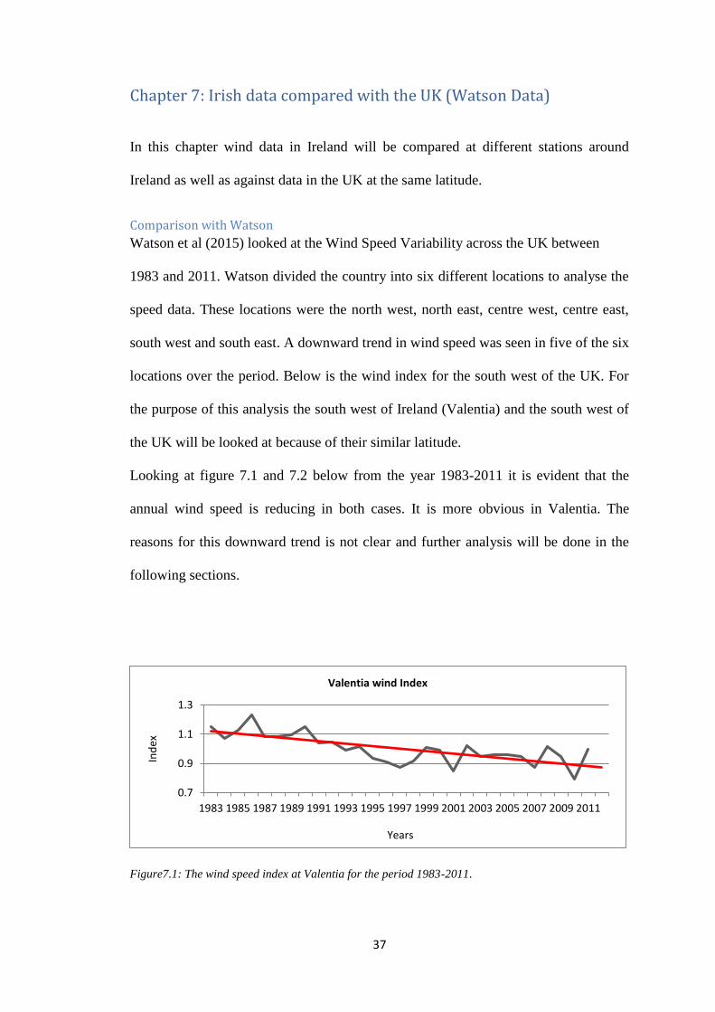
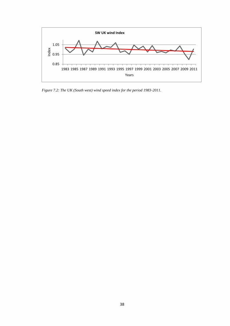
Chapter 7: Irish data compared with the UK (Watson Data)
In this chapter wind data in Ireland will be compared at different stations around
Ireland as well as against data in the UK at the same latitude.
Comparison with Watson
Watson et al (2015) looked at the Wind Speed Variability across the UK between
1983 and 2011. Watson divided the country into six different locations to analyse the
speed data. These locations were the north west, north east, centre west, centre east,
south west and south east. A downward trend in wind speed was seen in five of the six
locations over the period. Below is the wind index for the south west of the UK. For
the purpose of this analysis the south west of Ireland (Valentia) and the south west of
the UK will be looked at because of their similar latitude.
Looking at figure 7.1 and 7.2 below from the year 1983-2011 it is evident that the
annual wind speed is reducing in both cases. It is more obvious in Valentia. The
reasons for this downward trend is not clear and further analysis will be done in the
following sections.
Figure7.1: The wind speed index at Valentia for the period 1983-2011.
0.7
0.9
1.1
1.3
1983 1985 1987 1989 1991 1993 1995 1997 1999 2001 2003 2005 2007 2009 2011
Ind
ex
Years
Valentia wind Index
38
Figure 7.2: The UK (South west) wind speed index for the period 1983-2011.
0.85
0.95
1.05
1983 1985 1987 1989 1991 1993 1995 1997 1999 2001 2003 2005 2007 2009 2011
Ind
ex
Years
SW UK wind Index
39
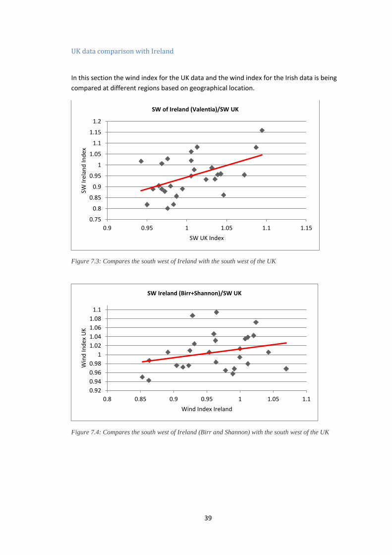
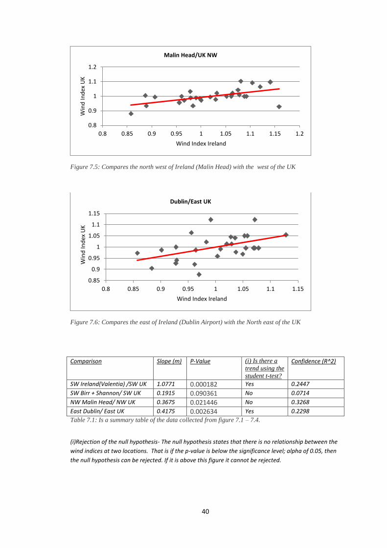
UK data comparison with Ireland
In this section the wind index for the UK data and the wind index for the Irish data is being
compared at different regions based on geographical location.
Figure 7.3: Compares the south west of Ireland with the south west of the UK
Figure 7.4: Compares the south west of Ireland (Birr and Shannon) with the south west of the UK
0.75
0.8
0.85
0.9
0.95
1
1.05
1.1
1.15
1.2
0.9 0.95 1 1.05 1.1 1.15
SW Ir
elan
d In
dex
SW UK Index
SW of Ireland (Valentia)/SW UK
0.92
0.94
0.96
0.98
1
1.02
1.04
1.06
1.08
1.1
0.8 0.85 0.9 0.95 1 1.05 1.1
Win
d In
dex
UK
Wind Index Ireland
SW Ireland (Birr+Shannon)/SW UK
40
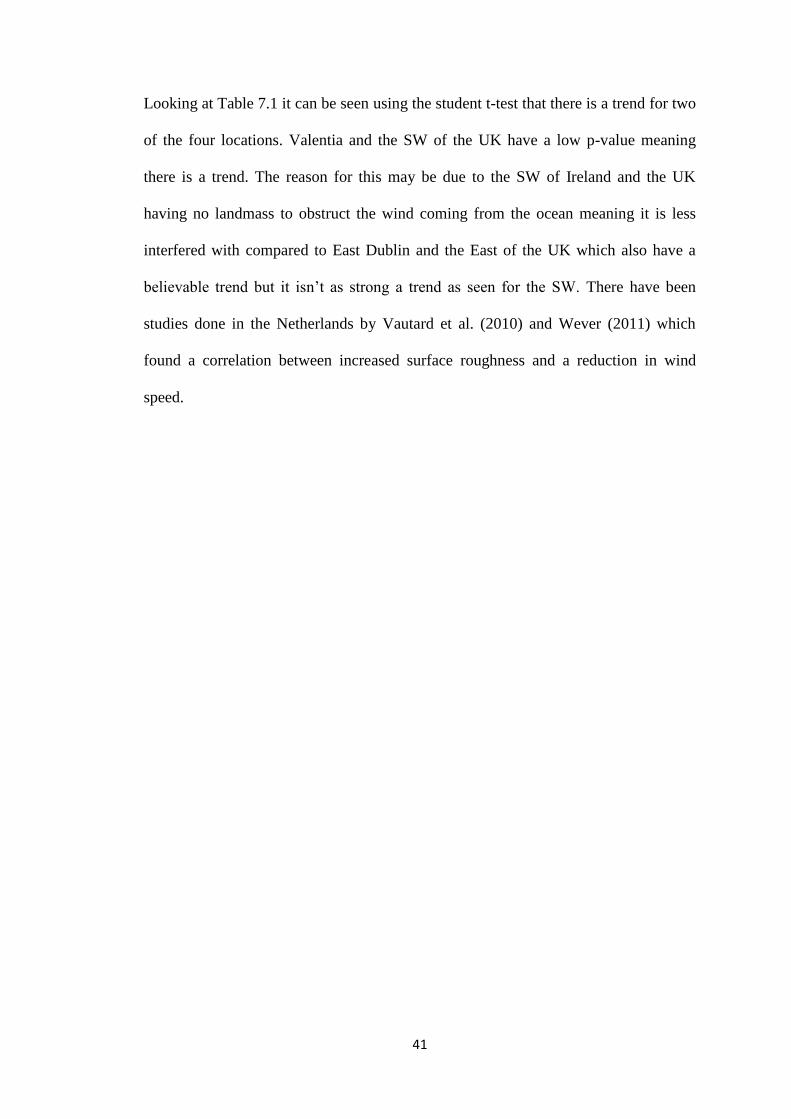
Figure 7.5: Compares the north west of Ireland (Malin Head) with the west of the UK
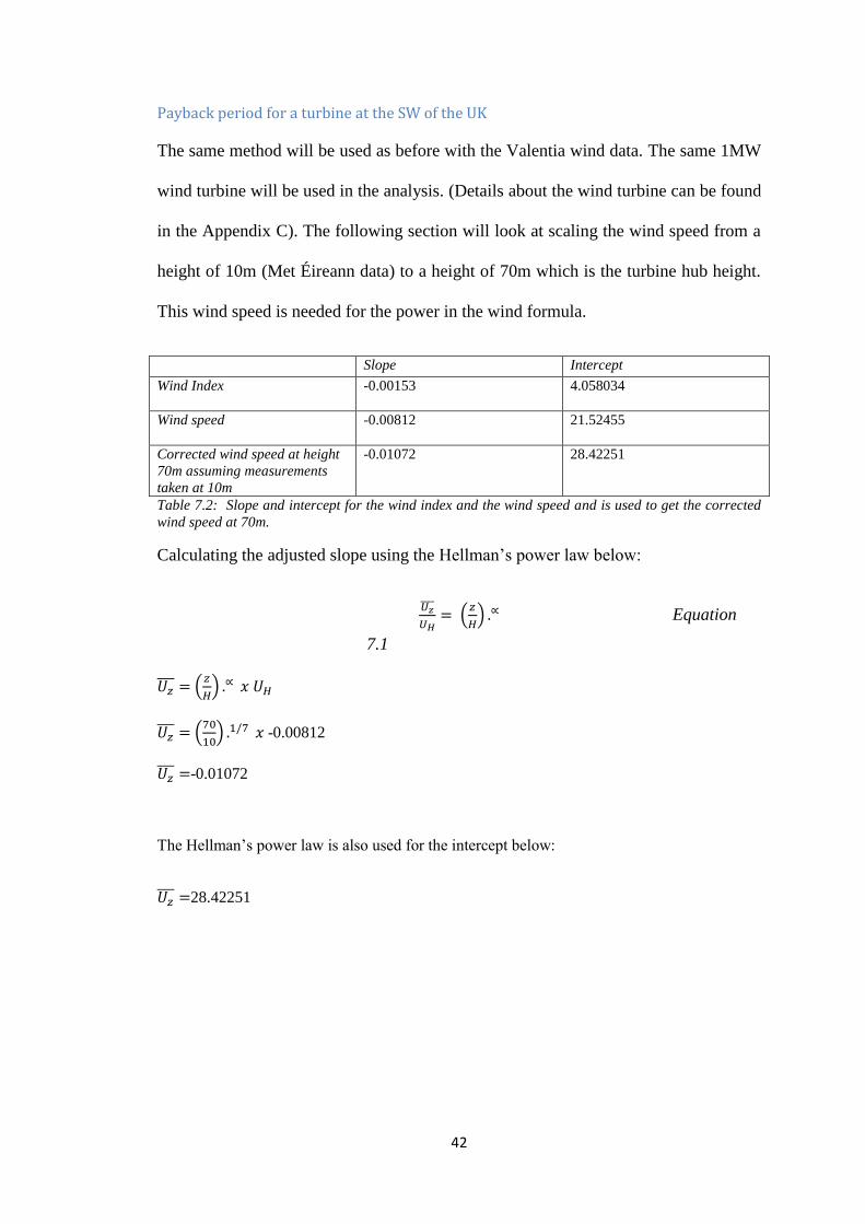
Figure 7.6: Compares the east of Ireland (Dublin Airport) with the North east of the UK
Comparison Slope (m) P-Value (i) Is there a
trend using the
student t-test?
Confidence (R^2)
SW Ireland(Valentia) /SW UK 1.0771 0.000182 Yes 0.2447
SW Birr + Shannon/ SW UK 0.1915 0.090361 No 0.0714
NW Malin Head/ NW UK 0.3675 0.021446 No 0.3268
East Dublin/ East UK 0.4175 0.002634 Yes 0.2298
Table 7.1: Is a summary table of the data collected from figure 7.1 – 7.4.
(i)Rejection of the null hypothesis- The null hypothesis states that there is no relationship between the
wind indices at two locations. That is if the p-value is below the significance level; alpha of 0.05, then
the null hypothesis can be rejected. If it is above this figure it cannot be rejected.
0.8
0.9
1
1.1
1.2
0.8 0.85 0.9 0.95 1 1.05 1.1 1.15 1.2
Win
d In
dex
UK
Wind Index Ireland
Malin Head/UK NW
0.85
0.9
0.95
1
1.05
1.1
1.15
0.8 0.85 0.9 0.95 1 1.05 1.1 1.15
Win
d In
dex
UK
Wind Index Ireland
Dublin/East UK
41
Looking at Table 7.1 it can be seen using the student t-test that there is a trend for two
of the four locations. Valentia and the SW of the UK have a low p-value meaning
there is a trend. The reason for this may be due to the SW of Ireland and the UK
having no landmass to obstruct the wind coming from the ocean meaning it is less
interfered with compared to East Dublin and the East of the UK which also have a
believable trend but it isn’t as strong a trend as seen for the SW. There have been
studies done in the Netherlands by Vautard et al. (2010) and Wever (2011) which
found a correlation between increased surface roughness and a reduction in wind
speed.
42
Payback period for a turbine at the SW of the UK
The same method will be used as before with the Valentia wind data. The same 1MW
wind turbine will be used in the analysis. (Details about the wind turbine can be found
in the Appendix C). The following section will look at scaling the wind speed from a
height of 10m (Met Éireann data) to a height of 70m which is the turbine hub height.
This wind speed is needed for the power in the wind formula.
Slope Intercept
Wind Index -0.00153
4.058034
Wind speed -0.00812
21.52455
Corrected wind speed at height
70m assuming measurements
taken at 10m
-0.01072
28.42251
Table 7.2: Slope and intercept for the wind index and the wind speed and is used to get the corrected
wind speed at 70m.
Calculating the adjusted slope using the Hellman’s power law below:
𝑈𝑧̅̅̅̅
𝑈𝐻= (
𝑧
𝐻) .∝ Equation
7.1
𝑈𝑧̅̅ ̅ = (
𝑧
𝐻) .∝ 𝑥 𝑈𝐻
𝑈𝑧̅̅ ̅ = (
70
10) .1/7 𝑥 -0.00812
𝑈𝑧̅̅ ̅ =-0.01072
The Hellman’s power law is also used for the intercept below:
𝑈𝑧̅̅ ̅ =28.42251
43
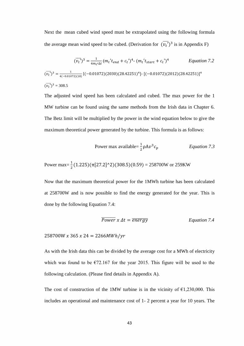
Next the mean cubed wind speed must be extrapolated using the following formula
the average mean wind speed to be cubed. (Derivation for (𝑣𝑡′̅̅̅̅ )3 is in Appendix F)
(𝑣𝑡′̅̅̅̅ )3 = 1
4𝑚𝑡′∆𝑡 (𝑚𝑡′𝑡𝑒𝑛𝑑 + 𝑐𝑡′)4- (𝑚𝑡′𝑡𝑠𝑡𝑎𝑟𝑡 + 𝑐𝑡′)4 Equation 7.2
(𝑣𝑡′̅̅̅̅ )3 = 1
4(−0.01072)(18) [(−0.01072)(2030)(28.42251)4]- [(−0.01072)(2012)(28.42251)]4
(𝑣𝑡′̅̅̅̅ )3 = 308.5
The adjusted wind speed has been calculated and cubed. The max power for the 1
MW turbine can be found using the same methods from the Irish data in Chapter 6.
The Betz limit will be multiplied by the power in the wind equation below to give the
maximum theoretical power generated by the turbine. This formula is as follows:
Power max available= 1
2ρA𝑣3𝑐𝑝 Equation 7.3
Power max= 1
2(1.225)(π[27.2]^2)(308.5)(0.59) = 258700W or 259KW
Now that the maximum theoretical power for the 1MWh turbine has been calculated
at 258700W and is now possible to find the energy generated for the year. This is
done by the following Equation 7.4:
𝑃𝑜𝑤𝑒𝑟̅̅ ̅̅ ̅̅ ̅̅ ̅ 𝑥 𝛥𝑡 = 𝑒𝑛𝑒𝑟𝑔𝑦̅̅ ̅̅ ̅̅ ̅̅ ̅̅ Equation 7.4
258700W 𝑥 365 𝑥 24 = 2266𝑀𝑊ℎ/𝑦𝑟
As with the Irish data this can be divided by the average cost for a MWh of electricity
which was found to be €72.167 for the year 2015. This figure will be used to the
following calculation. (Please find details in Appendix A).
The cost of construction of the 1MW turbine is in the vicinity of €1,230,000. This
includes an operational and maintenance cost of 1- 2 percent a year for 10 years. The
44
construction cost/operation/maintenance cost is now divided by the revenue for the
year to give the payback period in years as follows.
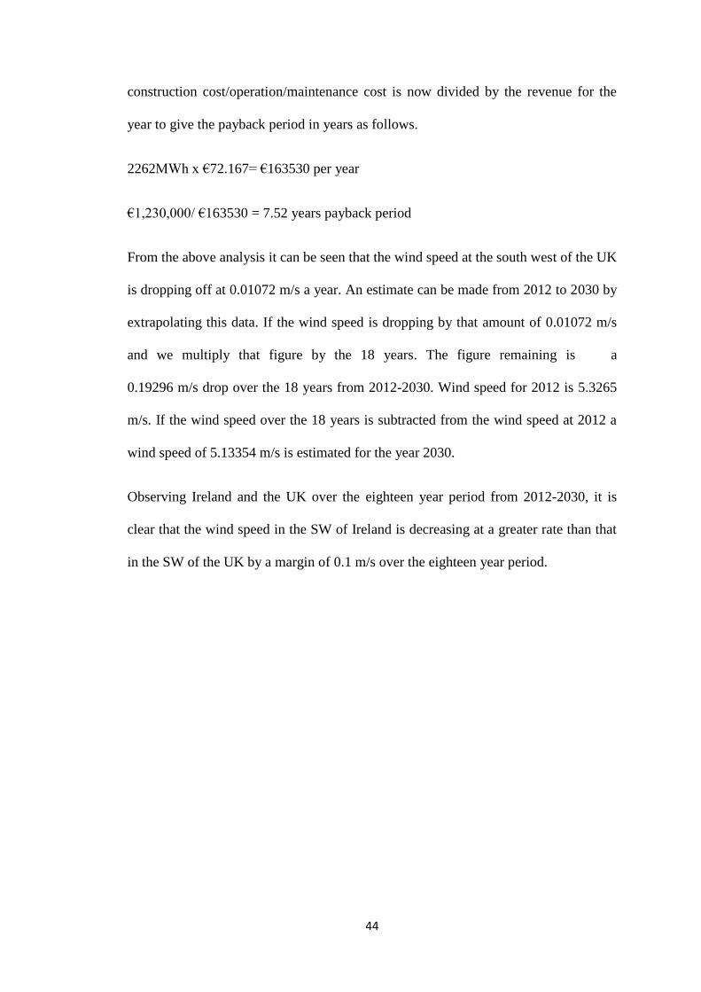
2262MWh x €72.167= €163530 per year
€1,230,000/ €163530 = 7.52 years payback period
From the above analysis it can be seen that the wind speed at the south west of the UK
is dropping off at 0.01072 m/s a year. An estimate can be made from 2012 to 2030 by
extrapolating this data. If the wind speed is dropping by that amount of 0.01072 m/s
and we multiply that figure by the 18 years. The figure remaining is a
0.19296 m/s drop over the 18 years from 2012-2030. Wind speed for 2012 is 5.3265
m/s. If the wind speed over the 18 years is subtracted from the wind speed at 2012 a
wind speed of 5.13354 m/s is estimated for the year 2030.
Observing Ireland and the UK over the eighteen year period from 2012-2030, it is
clear that the wind speed in the SW of Ireland is decreasing at a greater rate than that
in the SW of the UK by a margin of 0.1 m/s over the eighteen year period.
45
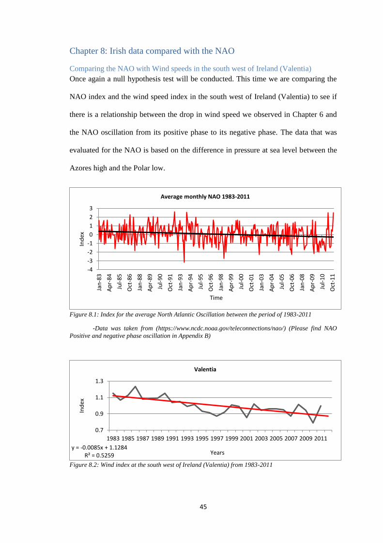
Chapter 8: Irish data compared with the NAO
Comparing the NAO with Wind speeds in the south west of Ireland (Valentia)
Once again a null hypothesis test will be conducted. This time we are comparing the
NAO index and the wind speed index in the south west of Ireland (Valentia) to see if
there is a relationship between the drop in wind speed we observed in Chapter 6 and
the NAO oscillation from its positive phase to its negative phase. The data that was
evaluated for the NAO is based on the difference in pressure at sea level between the
Azores high and the Polar low.
Figure 8.1: Index for the average North Atlantic Oscillation between the period of 1983-2011
-Data was taken from (https://www.ncdc.noaa.gov/teleconnections/nao/) (Please find NAO
Positive and negative phase oscillation in Appendix B)
Figure 8.2: Wind index at the south west of Ireland (Valentia) from 1983-2011
-4
-3
-2
-1
0
1
2
3
Jan
-83
Ap
r-8
4
Jul-
85
Oct
-86
Jan
-88
Ap
r-8
9
Jul-
90
Oct
-91
Jan
-93
Ap
r-9
4
Jul-
95
Oct
-96
Jan
-98
Ap
r-9
9
Jul-
00
Oct
-01
Jan
-03
Ap
r-0
4
Jul-
05
Oct
-06
Jan
-08
Ap
r-0
9
Jul-
10
Oct
-11
Ind
ex
Time
Average monthly NAO 1983-2011
y = -0.0085x + 1.1284R² = 0.5259
0.7
0.9
1.1
1.3
1983 1985 1987 1989 1991 1993 1995 1997 1999 2001 2003 2005 2007 2009 2011
Ind
ex
Years
Valentia
46
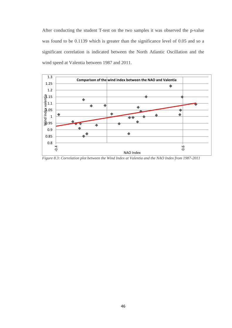
After conducting the student T-test on the two samples it was observed the p-value
was found to be 0.1139 which is greater than the significance level of 0.05 and so a
significant correlation is indicated between the North Atlantic Oscillation and the
wind speed at Valentia between 1987 and 2011.
Figure 8.3: Correlation plot between the Wind Index at Valentia and the NAO Index from 1987-2011
0.8
0.85
0.9
0.95
1
1.05
1.1
1.15
1.2
1.25
1.3
-0.4
0.6
Win
d In
dex
val
enti
a
NAO Index
Comparison of the wind index between the NAO and Valentia
47
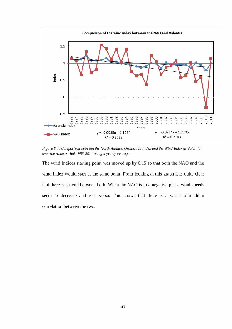
Figure 8.4: Comparison between the North Atlantic Oscillation Index and the Wind Index at Valentia
over the same period 1983-2011 using a yearly average.
The wind Indices starting point was moved up by 0.15 so that both the NAO and the
wind index would start at the same point. From looking at this graph it is quite clear
that there is a trend between both. When the NAO is in a negative phase wind speeds
seem to decrease and vice versa. This shows that there is a weak to medium
correlation between the two.
y = -0.0085x + 1.1284R² = 0.5259
y = -0.0214x + 1.2205R² = 0.2143
-0.5
0
0.5
1
1.5
19
83
19
84
19
85
19
86
19
87
19
88
19
89
19
90
19
91
19
92
19
93
19
94
19
95
19
96
19
97
19
98
19
99
20
00
20
01
20
02
20
03
20
04
20
05
20
06
20
07
20
08
20
09
20
10
20
11
Ind
ex
Years
Comparison of the wind index between the NAO and Valentia
Valentia index
NAO Index

48
Future predictions for the NAO
Burningham looks at the correlation between the NAO and Northern Europe
including Bellmullet, Malin Head and Valentia (Burningham et al 2013). He
mentions that “Average winter wind speed is weakly correlated with the NAO winter
index”. He says that 26 percent of the sites he examined had a strong correlation with
the winter NAO. This only applied to south westerly winds. At higher wind speeds he
noted that only 11 percent of the stations saw a correlation.
In times of a strong negative phase of the NAO the wind speeds tend to be lower and
the direction isn’t predominantly from the south westerly direction. This can be seen
on the NAO map in the appendix B for the winter of 2009/2010 where Northern
Europe saw its 18th coldest winter in history (Lockwood et al). Instead it is more
evenly spread out with a greater chance of north easterly winds. This is due to the
increase in pressure over the Arctic which slows down the wind speeds. On the other
hand when the NAO is in a strong positive phase winds tend to be stronger and
predominantly from the south west direction (Earl et al).
Visbeck et al. mention that at the current time there are no methods that can be used
for observing the low frequency variability of the NAO. This means uncertainty about
the NAO into the future. Visbeck talks about an increase in greenhouse gas emissions
and hence surface temperature may cause the positive index to continue in the
positive phase. The Met office at Hardley Centre is in an early stage of developing a
forecasting model for a negative phase NAO. They are using a large range forecast
model. The model could allow prediction for an increase or a decrease in wind speed
and at a certain rate. The problem with it is that it only looks at a short term period of
months ahead. To be able to predict a decrease or an increase in Ireland we need to
have the ability to look further ahead.
49
Chapter 9: Irish data compared with the Weibull Distribution
Valentia over 20 years
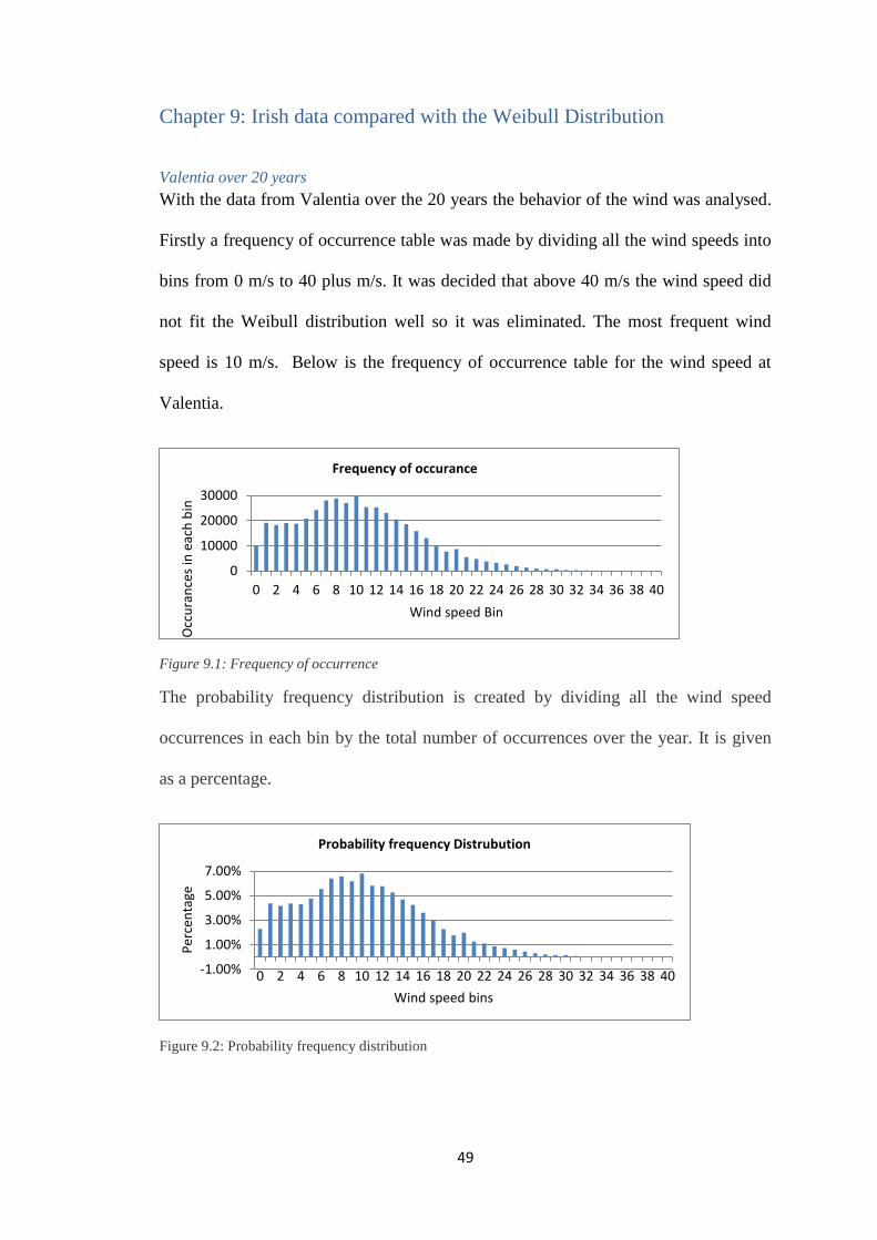
With the data from Valentia over the 20 years the behavior of the wind was analysed.
Firstly a frequency of occurrence table was made by dividing all the wind speeds into
bins from 0 m/s to 40 plus m/s. It was decided that above 40 m/s the wind speed did
not fit the Weibull distribution well so it was eliminated. The most frequent wind
speed is 10 m/s. Below is the frequency of occurrence table for the wind speed at
Valentia.
Figure 9.1: Frequency of occurrence
The probability frequency distribution is created by dividing all the wind speed
occurrences in each bin by the total number of occurrences over the year. It is given
as a percentage.
Figure 9.2: Probability frequency distribution
0
10000
20000
30000
0 2 4 6 8 10 12 14 16 18 20 22 24 26 28 30 32 34 36 38 40
Occ
ura
nce
s in
eac
h b
in
Wind speed Bin
Frequency of occurance
-1.00%
1.00%
3.00%
5.00%
7.00%
0 2 4 6 8 10 12 14 16 18 20 22 24 26 28 30 32 34 36 38 40
Per
cen
tage
Wind speed bins
Probability frequency Distrubution
50
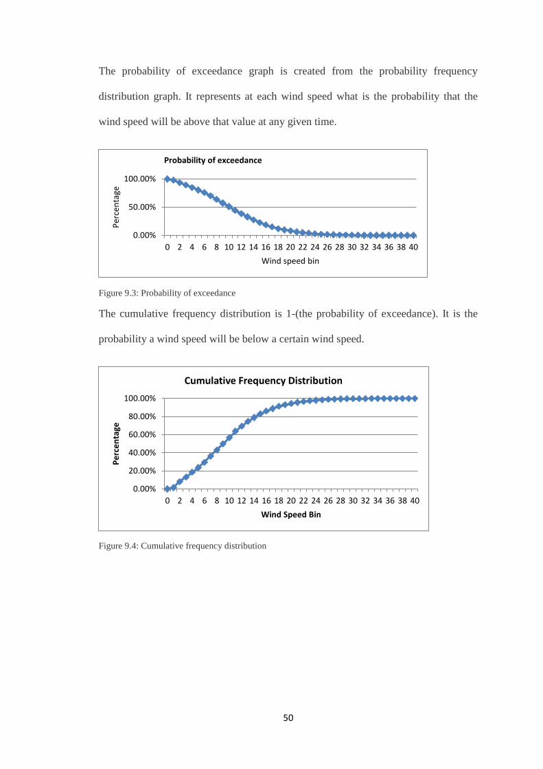
The probability of exceedance graph is created from the probability frequency
distribution graph. It represents at each wind speed what is the probability that the
wind speed will be above that value at any given time.
Figure 9.3: Probability of exceedance
The cumulative frequency distribution is 1-(the probability of exceedance). It is the
probability a wind speed will be below a certain wind speed.
Figure 9.4: Cumulative frequency distribution
0.00%
50.00%
100.00%
0 2 4 6 8 10 12 14 16 18 20 22 24 26 28 30 32 34 36 38 40
Per
cen
tage
Wind speed bin
Probability of exceedance
0.00%
20.00%
40.00%
60.00%
80.00%
100.00%
0 2 4 6 8 10 12 14 16 18 20 22 24 26 28 30 32 34 36 38 40
Pe
rce
nta
ge
Wind Speed Bin
Cumulative Frequency Distribution
51
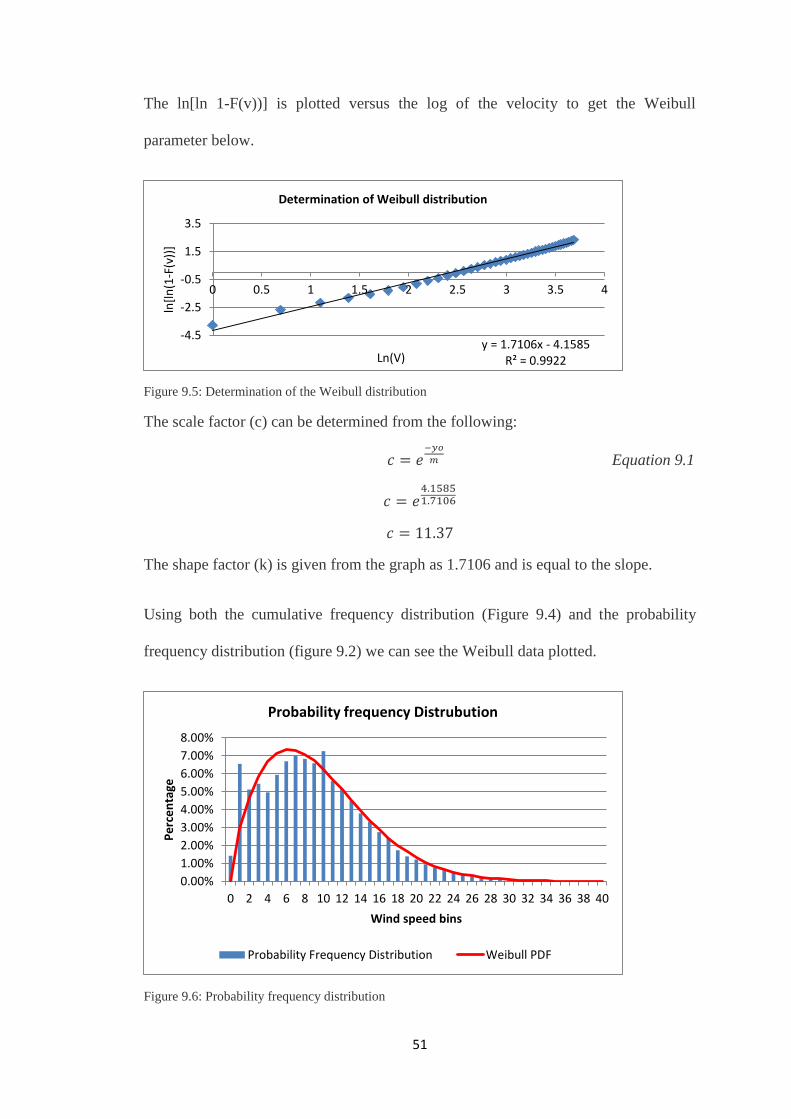
The ln[ln 1-F(v))] is plotted versus the log of the velocity to get the Weibull
parameter below.
Figure 9.5: Determination of the Weibull distribution
The scale factor (c) can be determined from the following:
𝑐 = 𝑒−𝑦𝑜
𝑚 Equation 9.1
𝑐 = 𝑒4.15851.7106
𝑐 = 11.37
The shape factor (k) is given from the graph as 1.7106 and is equal to the slope.
Using both the cumulative frequency distribution (Figure 9.4) and the probability
frequency distribution (figure 9.2) we can see the Weibull data plotted.
Figure 9.6: Probability frequency distribution
y = 1.7106x - 4.1585R² = 0.9922
-4.5
-2.5
-0.5
1.5
3.5
0 0.5 1 1.5 2 2.5 3 3.5 4
ln[l
n(1
-F(v
))]
Ln(V)
Determination of Weibull distribution
0.00%
1.00%
2.00%
3.00%
4.00%
5.00%
6.00%
7.00%
8.00%
0 2 4 6 8 10 12 14 16 18 20 22 24 26 28 30 32 34 36 38 40
Pe
rce
nta
ge
Wind speed bins
Probability frequency Distrubution
Probability Frequency Distribution Weibull PDF
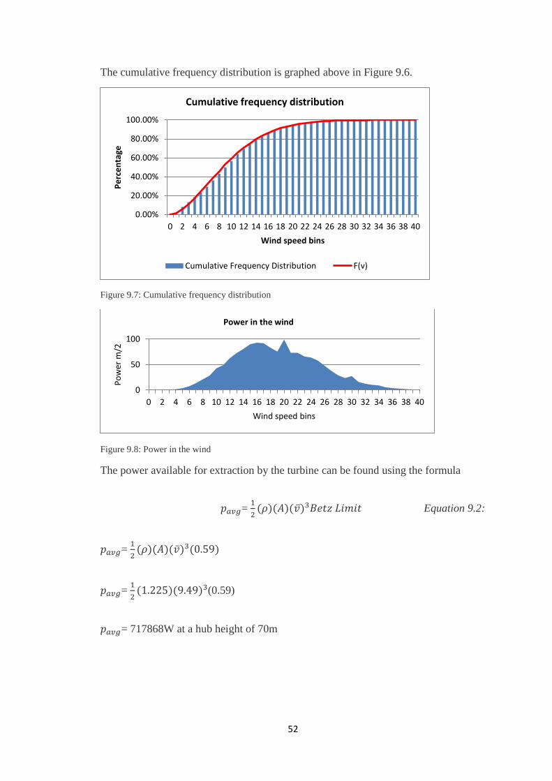
52
The cumulative frequency distribution is graphed above in Figure 9.6.
Figure 9.7: Cumulative frequency distribution
Figure 9.8: Power in the wind
The power available for extraction by the turbine can be found using the formula
𝑝𝑎𝑣𝑔= 1
2(𝜌)(𝐴)(�̅�)3𝐵𝑒𝑡𝑧 𝐿𝑖𝑚𝑖𝑡 Equation 9.2:
𝑝𝑎𝑣𝑔= 1
2(𝜌)(𝐴)(�̅�)3(0.59)
𝑝𝑎𝑣𝑔= 1
2(1.225)(9.49)3(0.59)
𝑝𝑎𝑣𝑔= 717868W at a hub height of 70m
0.00%
20.00%
40.00%
60.00%
80.00%
100.00%
0 2 4 6 8 10 12 14 16 18 20 22 24 26 28 30 32 34 36 38 40
Pe
rce
nta
ge
Wind speed bins
Cumulative frequency distribution
Cumulative Frequency Distribution F(v)
0
50
100
0 2 4 6 8 10 12 14 16 18 20 22 24 26 28 30 32 34 36 38 40
Po
wer
m/2
Wind speed bins
Power in the wind
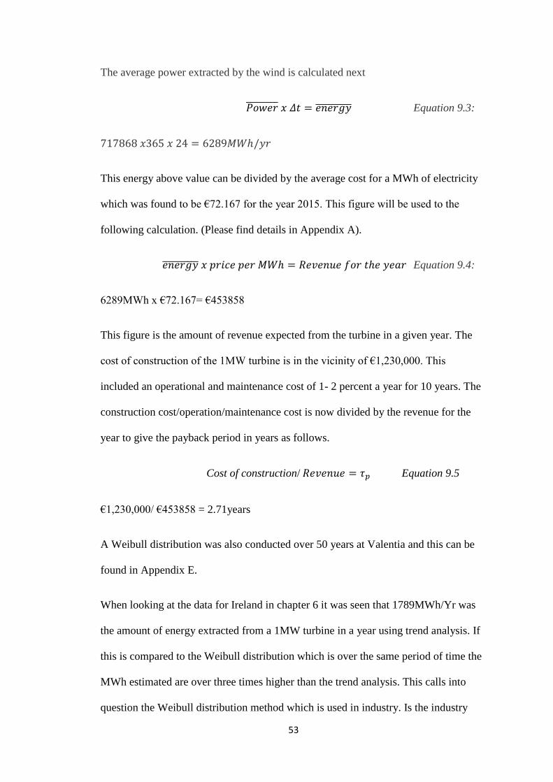
53
The average power extracted by the wind is calculated next
𝑃𝑜𝑤𝑒𝑟̅̅ ̅̅ ̅̅ ̅̅ ̅ 𝑥 𝛥𝑡 = 𝑒𝑛𝑒𝑟𝑔𝑦̅̅ ̅̅ ̅̅ ̅̅ ̅̅ Equation 9.3:
717868 𝑥365 𝑥 24 = 6289𝑀𝑊ℎ/𝑦𝑟
This energy above value can be divided by the average cost for a MWh of electricity
which was found to be €72.167 for the year 2015. This figure will be used to the
following calculation. (Please find details in Appendix A).
𝑒𝑛𝑒𝑟𝑔𝑦̅̅ ̅̅ ̅̅ ̅̅ ̅̅ 𝑥 𝑝𝑟𝑖𝑐𝑒 𝑝𝑒𝑟 𝑀𝑊ℎ = 𝑅𝑒𝑣𝑒𝑛𝑢𝑒 𝑓𝑜𝑟 𝑡ℎ𝑒 𝑦𝑒𝑎𝑟 Equation 9.4:
6289MWh x €72.167= €453858
This figure is the amount of revenue expected from the turbine in a given year. The
cost of construction of the 1MW turbine is in the vicinity of €1,230,000. This
included an operational and maintenance cost of 1- 2 percent a year for 10 years. The
construction cost/operation/maintenance cost is now divided by the revenue for the
year to give the payback period in years as follows.
Cost of construction/ 𝑅𝑒𝑣𝑒𝑛𝑢𝑒 = 𝜏𝑝 Equation 9.5
€1,230,000/ €453858 = 2.71years
A Weibull distribution was also conducted over 50 years at Valentia and this can be
found in Appendix E.
When looking at the data for Ireland in chapter 6 it was seen that 1789MWh/Yr was
the amount of energy extracted from a 1MW turbine in a year using trend analysis. If
this is compared to the Weibull distribution which is over the same period of time the
MWh estimated are over three times higher than the trend analysis. This calls into
question the Weibull distribution method which is used in industry. Is the industry

54
over-estimating the maximum energy the turbine extracted from the wind? From the
data it is quite evident that they are.
If we take a further look at the probability frequency distribution it is clear that the
Weibull does not fit the wind data perfectly. There are discrepancies where it does not
fit inside the Weibull PDF. This calls into question why this is the main method used
by industry for finding the power in the wind and hence the revenue and payback
period for a turbine.
56
Chapter 10: Conclusion
This paper set out to explore the characteristics and trends of wind in the South West
of Ireland in terms of its potential as a source of power generation.
Average wind speeds in the south west of Ireland, specifically in Valentia and
Shannon Airport, show a distinct downward trend since records began. A similar
trend is evident in wind data from the south west of the UK. A wide variation of
opinion exists regarding the influence of the NAO on wind strength in Northern
Europe. However this paper has illustrated a moderate level of confidence- 0.3968, in
a correlation of wind indices between Valentia and the NAO.
Despite the importance to the power generation industry of identifying trends in wind
variability, the industry uses a shorter (20 year) period than this paper used as a basis
for wind farm development. Trends evident in 50 year analyses in this paper are not
apparent in 20 year studies.
The Weibull distribution method- widely used by the wind-power industry, was
applied using Valentia wind data and this produced a scarcely credible 2.71 year
payback for a 1MW turbine. Once again this raises questions regarding the methods
used by the industry to evaluate wind energy projects.
However the payback period for a 1MW turbine using trend analysis for the region
was 9.53 years and this would become less attractive over time given the trend.
The potential of wind for power production, even in what appears to be the most
favourable part of the island of Ireland, is not yet proven and needs to be subjected to
more rigorous analysis by industry players
a
Bibliography
Atkinson, N, Harman, K, Lynn, M, Schwarz, A, Tindal, A. (2005) ‘Long-term wind
speed terms in north western Europe’.
Bakker, A and Van den Hurk, B. (2010) 'Estimation of persistence and trends in
geostrophic wind speed for the assessment of wind energy yields in Northwest
Europe' Volume 30(3), pp, 767-782.
Dwyer, N. Walsh, S (2012) “Surface winds” The status of Irelands Climate 2012,
EPA, University College Cork, Dwyer, 19-21 [accessed 14/09/15]
Department of Communications, Energy and Natural resources, Refit scheme and
supports, reference price. [available]
http://www.dcenr.gov.ie/energy/SiteCollectionDocuments/Renewable-
Energy/Refit%20Reference%20Prices.pdf [accessed 29/03/16]
Earl, N, Dorling, S, Hewston, R and Von Glasow,R. (2012) '1980–2010 Variability in
U.K. Surface Wind Climate', Volume 26, pp, 1172-1191.
Eberly College of Science, Statistics, Review of basic statistical concepts, 3.2
Hypothesis testing (p-value approach)
https://onlinecourses.science.psu.edu/statprogram/node/138 [accessed 8/11/15]
b
Enerpower, total energy solutions, available:
http://www.enerpower.ie/page/wind/wind-turbine-payback-period
http://etcgreen.com/horizontal-axis-wind-turbine-1mw/ [accessed 12/03/16]
ETCGREEN, Horizonal axis wind turbines – 1MW available:
http://etcgreen.com/horizontal-axis-wind-turbine-1mw/ [accessed 17/03/16]
Feldstein, S (2007) “The dynamics of the North Atlantic Oscillation during the
summer season” QUARTERLY JOURNAL OF THE ROYAL METEOROLOGICAL
SOCIETY, Pennsylvania State University, 1-4[accessed 21/09/15]
Lockwood, M., Harrison, R.G., Woollings, T. and Solanki, S.K., 2010. Are cold
winters in Europe associated with low solar activity?. Environmental Research
Letters, 5(2), p.024001
IWEA, Irish Wind Energy Association, Wind energy technology. Available:
http://www.iwea.com/index.cfm/page/technicalfaqs?#q32 [accessed 22/03/16]
Maps of World (2014) Irelands Latitude and Longitude maps available:
http://www.mapsofworld.com/lat_long/ireland-lat-long.html [accessed 14/09/2015]
Mcgrath, R. Lynch, P (June 2008) National Development Plan, Ireland in a warmer
world, Met Eireann, UCD Dublin, 35 [Accessed 16/09/15]
c
Met Éireann, Climate of Ireland (2015) available: http://www.met.ie/climate-
ireland/climate-of-ireland.asp [accessed 13/09/15]
Met Éireann (2009) Wind over Ireland, available:
http://www.met.ie/images/windrose/malin.png [accessed 13/09/15]
Met Éireann, Met Éireann Climate of 2011 (2011) available:
http://www.met.ie/climate/monthlyBulletins/Climate_2011.pdf [accessed 13/09/15]
NASA, Ocean Motion, Ocean in Motion: Ekman Transport Background, available:
http://oceanmotion.org/images/ocean-in-motion_clip_image001.jpg [Accessed
17/9/15]
National Oceanic and Atmospheric Administration, Surface Ocean Currents, Ekman
spiral,available: http://oceanservice.noaa.gov/education/kits/currents/05currents4.html
[Accessed 22/9/15]
National centre for environmental information, Climate Monitoring, North Atlantic
Oscillation https://www.ncdc.noaa.gov/teleconnections/nao/ [accessed 8/11/2015]
National Ocean Service (2008) Currents, available:
http://oceanservice.noaa.gov/education/kits/currents/05currents2.html [accessed
14/09/15]

d
Nolan, P, Lynch, P, McGrath, R, Semmler, T and Wang, S. (2011) ‘Simulating
climate change and its effects on the wind energy resource of Ireland’, Volume 15(4),
pp. 593–608.
Persson, A. (2011) The Coriolis Effect – a conflict between common sense and
mathematics, Norrköping, Sweden, 3-6 [accessed 14/09/15]
Reilly,J. (2014) Why has it been so wet and so windy for so long?, 13/12/14 available:
http://www.independent.ie/irish-news/we-can-blame-the-jet-stream-for-our-wild-
weather-30005310.html [accessed 13/9/15]
Real Statistics using Excel, available: http://www.real-
statistics.com/regression/hypothesis-testing-significance-regression-
lineslope/comparing-slopes-two-independent-samples/ [accessed 6/11/2015]
Real Statistics using Excel, available: http://www.real-
statistics.com/regression/hypothesis-testing-significance-regression-line-slope/
[accessed 3/3/2016]
Rohan, k.P (1986) The Climate of Ireland, Dublin, 146 [Accessed 28/09/2015]
Ahrens, C. Donald (10th addition) Meteorology Today, An introduction to weather,
climate and the environment [accessed 03/10/15]
Single Energy Market Operator, available: http://www.sem-o.com/Pages/default.aspx
[accessed 16/03/16]
e
State Climate office of North Carolina, Global Patterns - Arctic & North Atlantic
Oscillations (AO & NAO), Arctic Oscillation (AO) available:
https://climate.ncsu.edu/climate/patterns/NAO.html [accessed 16/9/15]
Stull, R. (2000) ‘Meteorology for Scientists and Engineers’, second edition, pp, 184-
186. Sustainable Energy Authority of Ireland, Technology of wind energy, choosing a
wind turbine, available:
http://www.seai.ie/Renewables/Wind_Energy/Technology_of_Wind_Energy/
[accessed 19/03/16]
Vautard, R, Cattiaux, J, Yiou, P, Thépaut and J.N, Ciais,P. (2010) ‘Northern
Hemisphere atmospheric stilling partly attributed to an increase in surface roughness’
Nature Geoscience 3, pp, 756–761.
Visbeck, M, Hurrell, J, Polvani, L and Cullen, H. (2001) ‘The North Atlantic
Oscillation: Past, present, and future’, volume 98, pp, 23-24.
Watson, S, J, Kritharas, P and Hodgson, G.J. (2015), Wind speed variability across
the UK between 1957 and 2011, Volume 18(1), pp. 21-42.
Wever, N. (2012) 'Quantifying trends in surface roughness and the effect on surface
wind speed observations' Volume 117(D11).

f
Widén, J, Carpman, N, Castellucci,V, Lingfors,D, Olauson,J, Remouit, F, Bergkvist,
M, Grabbe,M and Waters, R. (2015) 'Variability assessment and forecasting of
renewables: A review for solar, wind, wave and tidal resources', volume 44, pp, 356-
375.
Walsh. P, ‘Wind Ocean and Hydro Energy’ ‘Velocity scaling with height’ pp, 133-
140
Walsh. P, ‘Wind Ocean and Hydro Energy’ ‘Wind Statistics’ pp, 159- 160
Walsh. P, ‘Wind Ocean and Hydro Energy’ ‘Weibull distribution pp, 165- 197
World Wind Patterns (2011) Global Wind Patterns, available:
http://deckskills.org/sitebuildercontent/sitebuilderpictures/global_wind_diagram.jpg
[accessed 13/09/15]
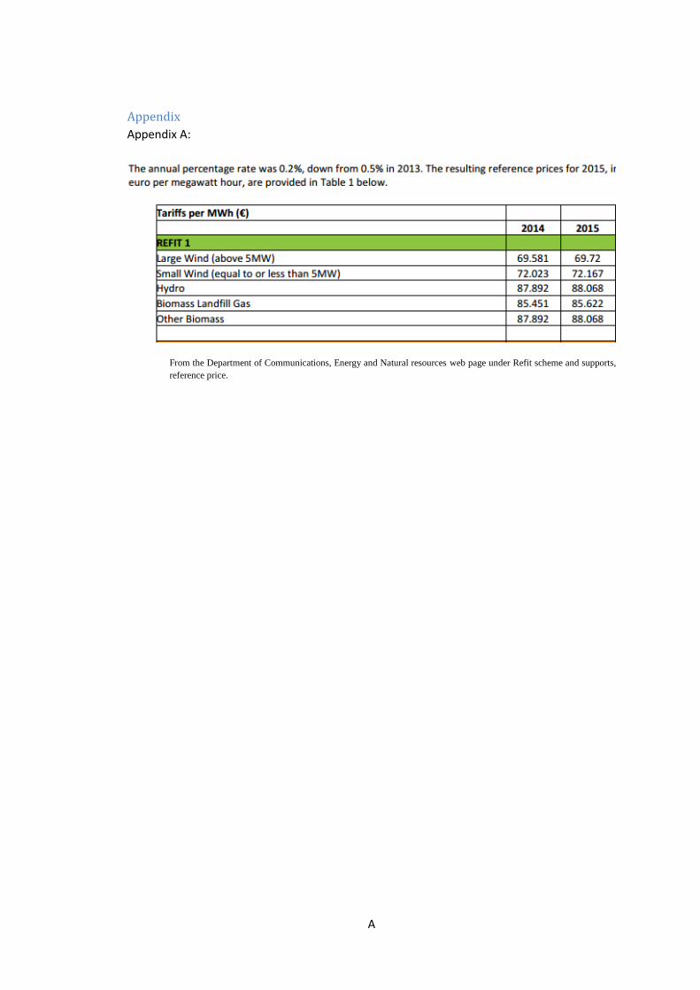
A
Appendix
Appendix A:
From the Department of Communications, Energy and Natural resources web page under Refit scheme and supports,
reference price.
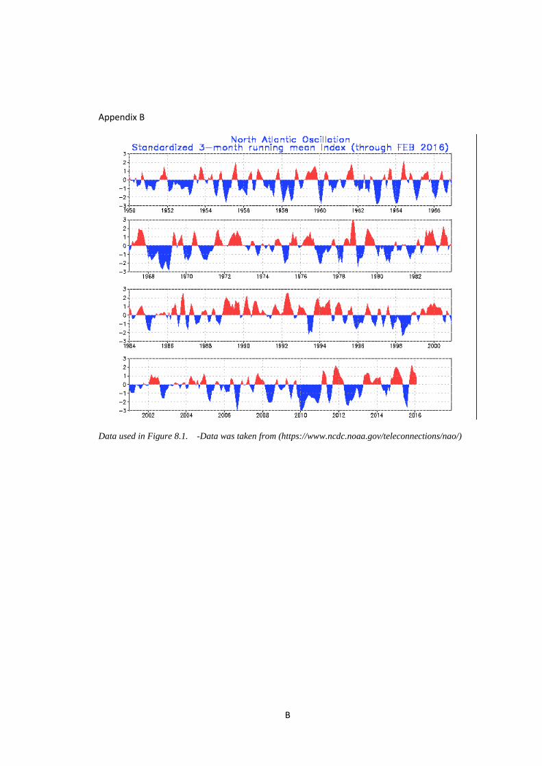
B
Appendix B
Data used in Figure 8.1. -Data was taken from (https://www.ncdc.noaa.gov/teleconnections/nao/)

C
Appendix C

D
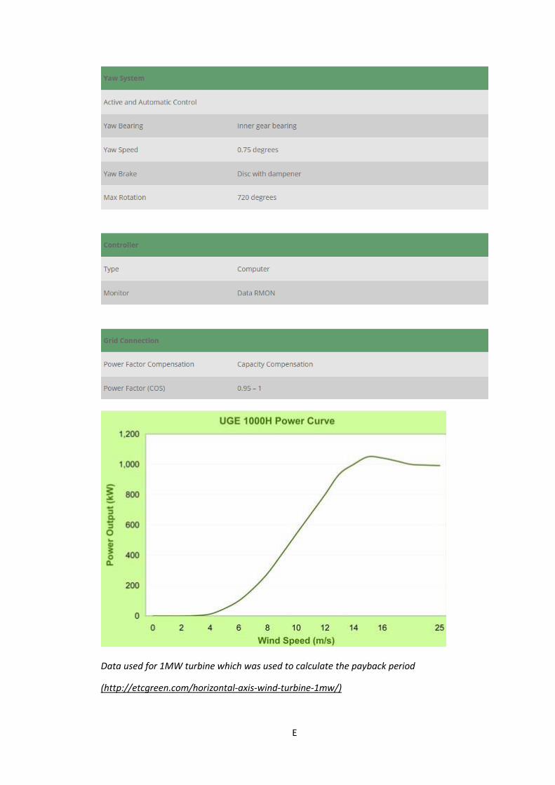
E
Data used for 1MW turbine which was used to calculate the payback period
(http://etcgreen.com/horizontal-axis-wind-turbine-1mw/)
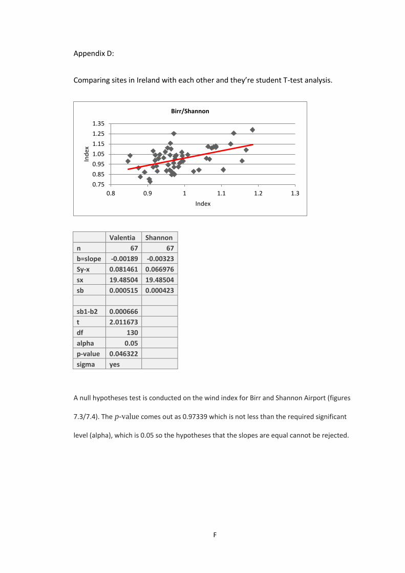
F
Appendix D:
Comparing sites in Ireland with each other and they’re student T-test analysis.
Valentia Shannon
n 67 67
b=slope -0.00189 -0.00323
Sy-x 0.081461 0.066976
sx 19.48504 19.48504
sb 0.000515 0.000423
sb1-b2 0.000666
t 2.011673
df 130
alpha 0.05
p-value 0.046322
sigma yes
A null hypotheses test is conducted on the wind index for Birr and Shannon Airport (figures
7.3/7.4). The p-value comes out as 0.97339 which is not less than the required significant
level (alpha), which is 0.05 so the hypotheses that the slopes are equal cannot be rejected.
0.75
0.85
0.95
1.05
1.15
1.25
1.35
0.8 0.9 1 1.1 1.2 1.3
Ind
ex
Index
Birr/Shannon
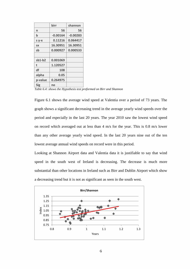
G
birr shannon
n 56 56
b -0.00164 -0.00283
s y-x 0.11216 0.064417
sx 16.30951 16.30951
sb 0.000927 0.000533
sb1-b2 0.001069
t 1.120527
df 108
alpha 0.05
p-value 0.264975
Sig no Table 6.4: shows the Hypothesis test preformed on Birr and Shannon
Figure 6.1 shows the average wind speed at Valentia over a period of 73 years. The
graph shows a significant decreasing trend in the average yearly wind speeds over the
period and especially in the last 20 years. The year 2010 saw the lowest wind speed
on record which averaged out at less than 4 m/s for the year. This is 0.8 m/s lower
than any other average yearly wind speed. In the last 20 years nine out of the ten
lowest average annual wind speeds on record were in this period.
Looking at Shannon Airport data and Valentia data it is justifiable to say that wind
speed in the south west of Ireland is decreasing. The decrease is much more
substantial than other locations in Ireland such as Birr and Dublin Airport which show
a decreasing trend but it is not as significant as seen in the south west.
0.75
0.85
0.95
1.05
1.15
1.25
1.35
0.8 0.9 1 1.1 1.2 1.3
Ind
ex
Years
Birr/Shannon
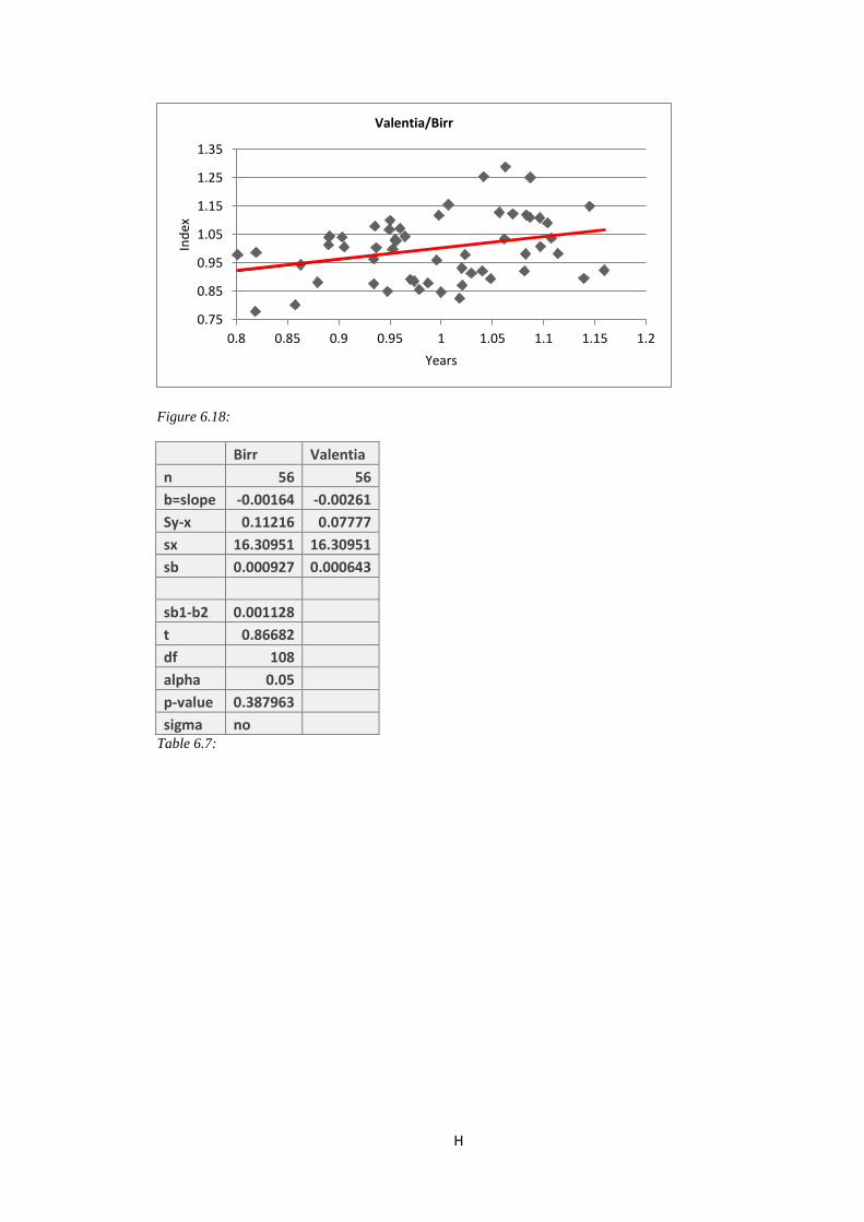
H
Figure 6.18:
Birr Valentia
n 56 56
b=slope -0.00164 -0.00261
Sy-x 0.11216 0.07777
sx 16.30951 16.30951
sb 0.000927 0.000643
sb1-b2 0.001128
t 0.86682
df 108
alpha 0.05
p-value 0.387963
sigma no Table 6.7:
0.75
0.85
0.95
1.05
1.15
1.25
1.35
0.8 0.85 0.9 0.95 1 1.05 1.1 1.15 1.2
Ind
ex
Years
Valentia/Birr
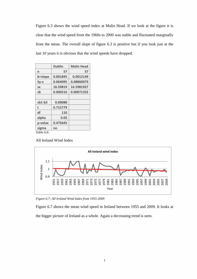
I
0.9
1
1.1
19
55
19
57
19
59
19
61
19
63
19
65
19
67
19
69
19
71
19
73
19
75
19
77
19
79
19
81
19
83
19
85
19
87
19
89
19
91
19
93
19
95
19
97
19
99
20
01
20
03
20
05
20
07
20
09W
ind
Ind
ex
Year
All Ireland wind index
Figure 6.3 shows the wind speed index at Malin Head. If we look at the figure it is
clear that the wind speed from the 1960s to 2000 was stable and fluctuated marginally
from the mean. The overall slope of figure 6.3 is positive but if you look just at the
last 10 years it is obvious that the wind speeds have dropped.
Dublin Malin Head
n 57 57
b=slope 0.001845 0.0012149
Sy-x 0.064095 0.08860079
sx 16.59819 16.5981927
sb 0.000516 0.00071332
sb1-b2 0.00088
t 0.715779
df 110
alpha 0.05
p-value 0.475645
sigma no Table 6.6:
All Ireland Wind Index
Figure 6.7: All Ireland Wind Index from 1955-2009
Figure 6.7 shows the mean wind speed in Ireland between 1955 and 2009. It looks at
the bigger picture of Ireland as a whole. Again a decreasing trend is seen.
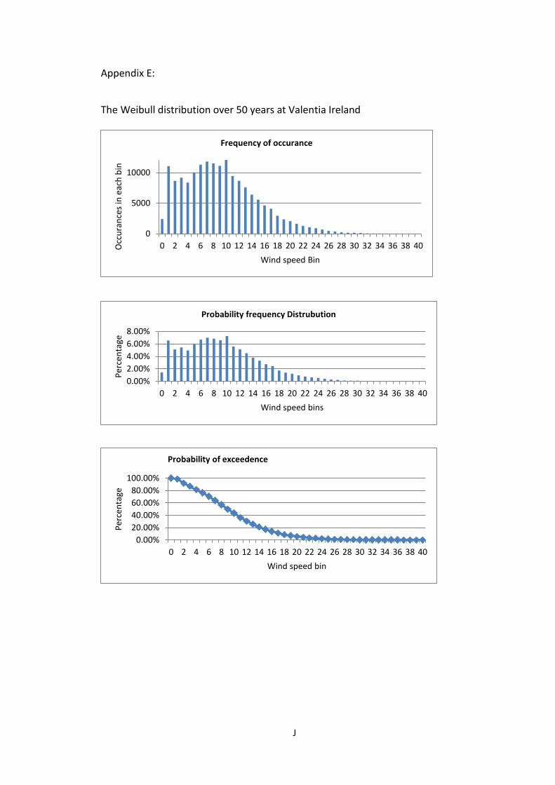
J
Appendix E:
The Weibull distribution over 50 years at Valentia Ireland
0
5000
10000
0 2 4 6 8 10 12 14 16 18 20 22 24 26 28 30 32 34 36 38 40Occ
ura
nce
s in
eac
h b
in
Wind speed Bin
Frequency of occurance
0.00%
2.00%
4.00%
6.00%
8.00%
0 2 4 6 8 10 12 14 16 18 20 22 24 26 28 30 32 34 36 38 40
Per
cen
tage
Wind speed bins
Probability frequency Distrubution
0.00%
20.00%
40.00%
60.00%
80.00%
100.00%
0 2 4 6 8 10 12 14 16 18 20 22 24 26 28 30 32 34 36 38 40
Per
cen
tage
Wind speed bin
Probability of exceedence
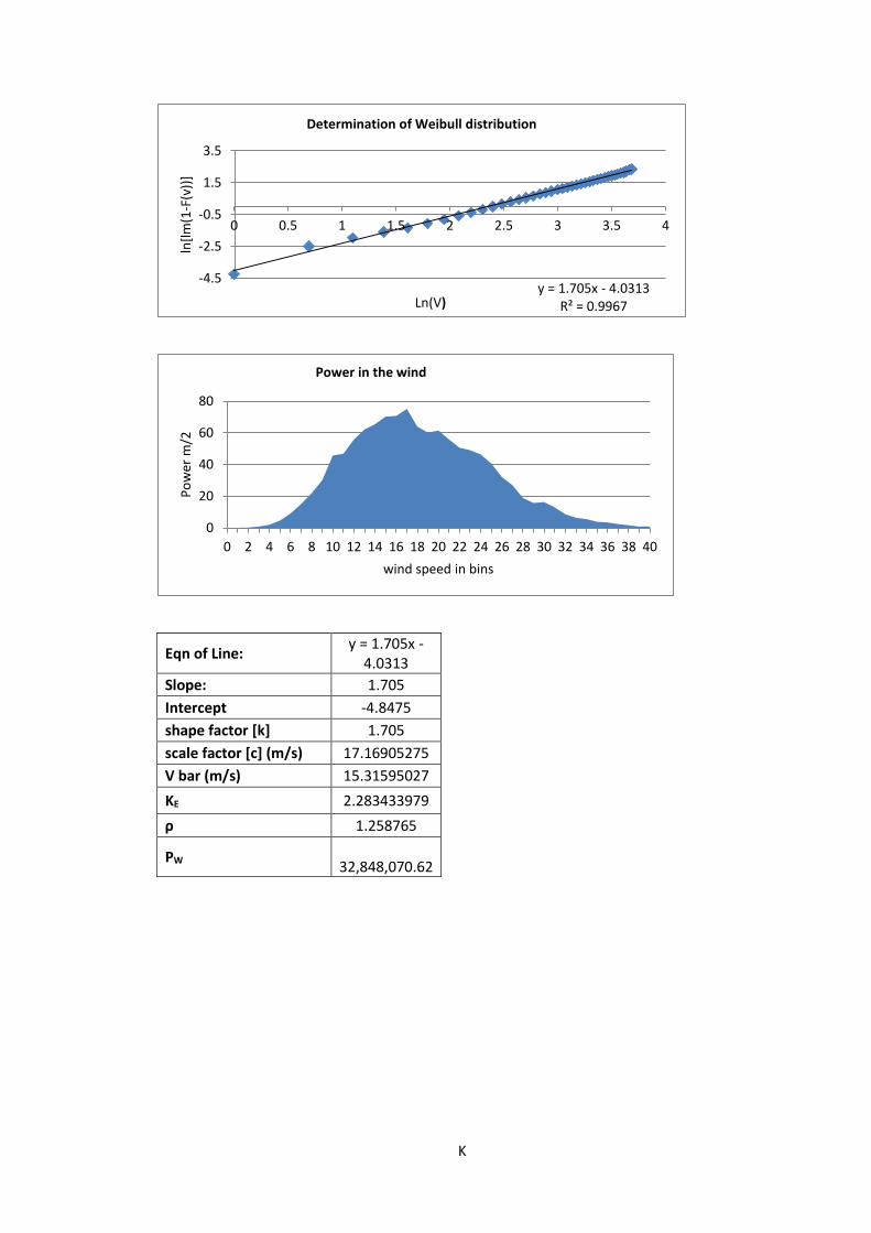
K
Eqn of Line: y = 1.705x -
4.0313
Slope: 1.705
Intercept -4.8475
shape factor [k] 1.705
scale factor [c] (m/s) 17.16905275
V bar (m/s) 15.31595027
KE 2.283433979
ρ 1.258765
PW
32,848,070.62
y = 1.705x - 4.0313R² = 0.9967
-4.5
-2.5
-0.5
1.5
3.5
0 0.5 1 1.5 2 2.5 3 3.5 4
ln[l
m(1
-F(v
))]
Ln(V)
Determination of Weibull distribution
0
20
40
60
80
0 2 4 6 8 10 12 14 16 18 20 22 24 26 28 30 32 34 36 38 40
Po
wer
m/2
wind speed in bins
Power in the wind
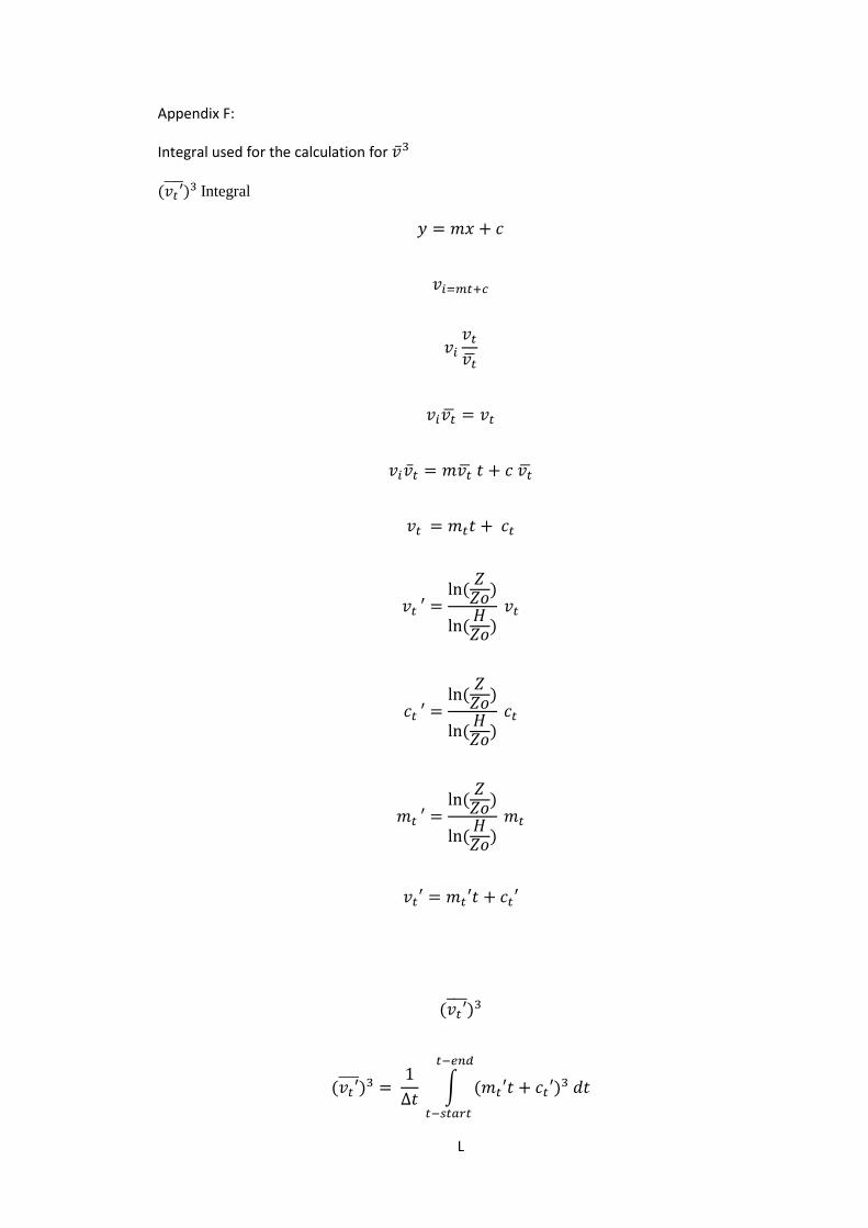
L
Appendix F:
Integral used for the calculation for �̅�3
(𝑣𝑡′̅̅̅̅ )3 Integral
𝑦 = 𝑚𝑥 + 𝑐
𝑣𝑖=𝑚𝑡+𝑐
𝑣𝑖
𝑣𝑡
𝑣�̅�
𝑣𝑖𝑣�̅� = 𝑣𝑡
𝑣𝑖�̅�𝑡 = 𝑚𝑣�̅� 𝑡 + 𝑐 𝑣�̅�
𝑣𝑡 = 𝑚𝑡𝑡 + 𝑐𝑡
𝑣𝑡 ′ =ln (
𝑍𝑍𝑜)
ln (𝐻𝑍𝑜)
𝑣𝑡
𝑐𝑡 ′ =ln (
𝑍𝑍𝑜)
ln (𝐻𝑍𝑜)
𝑐𝑡
𝑚𝑡 ′ =ln (
𝑍𝑍𝑜)
ln (𝐻𝑍𝑜)
𝑚𝑡
𝑣𝑡′ = 𝑚𝑡′𝑡 + 𝑐𝑡′
(𝑣𝑡′̅̅̅̅ )3
(𝑣𝑡′̅̅̅̅ )3 = 1
∆𝑡 ∫ (𝑚𝑡′𝑡 + 𝑐𝑡′)3 𝑑𝑡
𝑡−𝑒𝑛𝑑
𝑡−𝑠𝑡𝑎𝑟𝑡
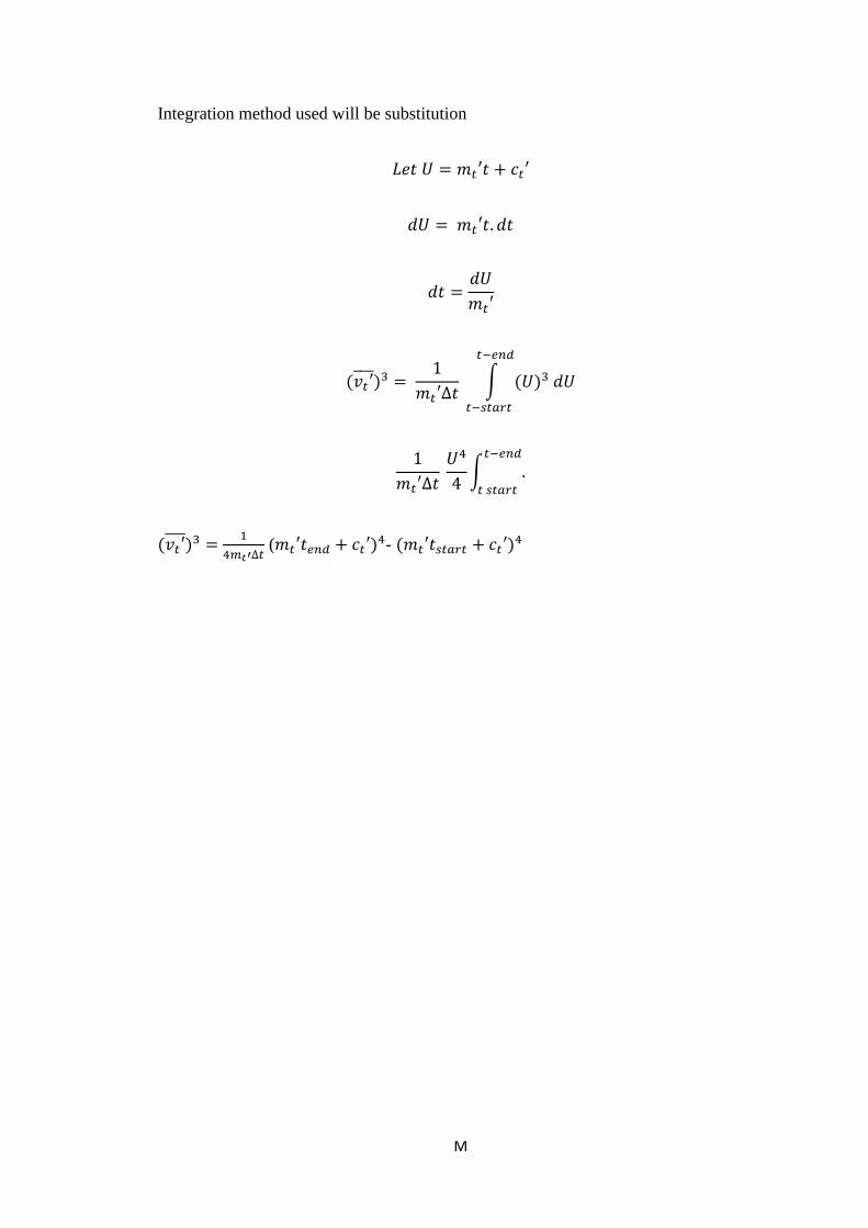
M
Integration method used will be substitution
𝐿𝑒𝑡 𝑈 = 𝑚𝑡′𝑡 + 𝑐𝑡′
𝑑𝑈 = 𝑚𝑡′𝑡. 𝑑𝑡
𝑑𝑡 =𝑑𝑈
𝑚𝑡′
(𝑣𝑡′̅̅̅̅ )3 = 1
𝑚𝑡′∆𝑡 ∫ (𝑈)3 𝑑𝑈
𝑡−𝑒𝑛𝑑
𝑡−𝑠𝑡𝑎𝑟𝑡
1
𝑚𝑡′∆𝑡 𝑈4
4∫ .
𝑡−𝑒𝑛𝑑
𝑡 𝑠𝑡𝑎𝑟𝑡
(𝑣𝑡′̅̅̅̅ )3 = 1
4𝑚𝑡′∆𝑡 (𝑚𝑡′𝑡𝑒𝑛𝑑 + 𝑐𝑡′)4- (𝑚𝑡′𝑡𝑠𝑡𝑎𝑟𝑡 + 𝑐𝑡′)4

N
Appendix F:
Comparing payback period at Valentia between 1939 and 2012
The average drop in wind speed from 1939-2012 in Valentia is -0.0146 m/s per a year.
When this is multiplied by 74 years it can be seen that there is a -1.08 m/s decrease in wind
speed since 1939. Wind speed at 1939 was 5.89 m/s on average and wind speed at 2012 was
1.08 less than that at 4.81.
1939
𝑥
5.89 =
𝑙𝑛(70
0.01)
𝑙𝑛(10
0.01) = 7.55 m/s
Next the maximum theoretical power can be found at this wind speed using the
following formula.
Power max= 1
2(1.225)(π[27.2]^2)(7.553)(0.59) = 361482 or 361KW
How much energy can this turbine produce in a year?
𝑃𝑜𝑤𝑒𝑟̅̅ ̅̅ ̅̅ ̅̅ ̅ 𝑥 𝛥𝑡 𝑥 𝐶𝑎𝑝𝑎𝑐𝑖𝑡𝑦 𝑓𝑎𝑐𝑡𝑜𝑟 = 𝑒𝑛𝑒𝑟𝑔𝑦̅̅ ̅̅ ̅̅ ̅̅ ̅̅
361482W 𝑥 365 𝑥 24 = 3167𝑀𝑊ℎ 𝑖𝑛 𝑎 𝑦𝑒𝑎𝑟
€50 for MWh (from SEMO website)
Cost of infrastructure for the turbine- €1,230,000
So 3167MWh x €50= €158350 per year
€1,230,000/ €158350 = 7.77years payback period

O
2012
𝑥
4.81 =
𝑙𝑛(70
0.01)
𝑙𝑛(10
0.01) = 6.16 m/s
Next the maximum theoretical power can be found at this wind speed using the
following formula.
Power max= 1
2(1.225)(π[27.2]^2)(6.163)(0.59) = 196331 or 196KW
How much energy can this turbine produce in a year?
𝑃𝑜𝑤𝑒𝑟̅̅ ̅̅ ̅̅ ̅̅ ̅ 𝑥 𝛥𝑡 𝑥 𝐶𝑎𝑝𝑎𝑐𝑖𝑡𝑦 𝑓𝑎𝑐𝑡𝑜𝑟 = 𝑒𝑛𝑒𝑟𝑔𝑦̅̅ ̅̅ ̅̅ ̅̅ ̅̅
196331W 𝑥 365 𝑥 24 = 1720𝑀𝑊ℎ 𝑖𝑛 𝑎 𝑦𝑒𝑎𝑟
€50 for MWh (from SEMO website)
Cost of infrastructure for the turbine- €1,230,000
So 1720MWhx €50= €86000 per year
€1,230,000/ €86000 = 14.3 years payback period
That is a payback difference between 1939 and 2012 of 6.53 years for a 1MW
turbine with a reduction in wind speed of just over 1 m/s on average.