Robot Motion Planning for Pouring Liquids

Zherong Pan, Chonhyon Park, Dinesh Manocha *

Abstract

We present a new algorithm to compute a collision-free tra-jectory for a robot manipulator to pour liquid from one con-tainer to the other. Our formulation uses a physical fluidmodel to predicate its highly deformable motion. We presentsimulation guided and optimization based method to auto-matically compute the transferring trajectory. Instead of ab-stract or simplified liquid models, we use the full-featured andaccurate Navier-Stokes model that provides the fine-grainedinformation of velocity distribution inside the liquid body.Moreover, this information is used as an additional guidingenergy term for the planner. One of our key contributions isthe tight integration between the fine-grained fluid simulator,liquid transfer controller, and the optimization-based planner.We have implemented the method using hybrid particle-meshfluid simulator (FLIP) and demonstrated its performance on4 benchmarks, with different cup shapes and viscosity coeffi-cients.

1 IntroductionRobotic manipulation of non-rigid and physical deformableobjects has been an active area of research. It frequentlyarises in industrial and medical applications. Most priorwork in this context has been related to picking flexible ob-jects, cable placement, surgical procedural planning, fold-ing clothes, etc. The resulting planners deal with issues re-lated to collision-free path computation as well as reliablephysics-based simulation of deformable objects.

In this paper, we address the problem of automaticallypouring liquids from one container to the other using robotmanipulators. Pouring liquids is a special case of a fluid ma-nipulation tasks that frequently arises in manufacturing ap-plications, corresponding to dispensing of adhesives, clean-ing of parts, lubricant changes, batch material handling in-cluding fluids, etc. Other applications include service robotsbeing used for daily chores such as cooking, cleaning orfeeding at home. One of the main challenges in these ap-plications is modeling the motion of the fluid and takingits deformable dynamics constraints into account as part of

*Zherong, Chonhyon and Dinesh are with Departmentof Computer Science, the University of North Carolina,{zherong,chpark,dm}@cs.unc.eduCopyright © 2016, Association for the Advancement of ArtificialIntelligence (www.aaai.org). All rights reserved.

Figure 1: An example of liquid transfer task performed by 7-DOF ClamArm robot. We use an optimization-based plan-ner that is tightly coupled with a fluid simulator and fluidtransfer controller.trajectory planning. In order to accurately model the fluid,we need to solve the governing nonlinear partial differen-tial equation, which can be a computationally challenging.Prior works on motion planning with fluid constraints (Davis2008; Kuriyama, Yano, and Hamaguchi 2008) use rathersimple fluid models or are based on imitation-based learn-ing (Langsfeld et al. 2014). However, their capabilities arelimited. No good solutions are known for accurately model-ing and planning the tasks of fluid pouring using robots.Main Results: We present a novel algorithm foroptimization-based planning that takes into accountconstraints corresponding to pouring liquids. Oneof key contributions is the tight integration betweenthe fine-grained fluid simulator and the optimization-based planner. We use an accurate particle-based fluidrepresentation that has been used for accurate andfine-grained modeling of fluids (Barreiro et al. 2013;Ihmsen et al. 2014). The complexity of particle-based fluidscan be high and it can take minutes to simulate a singletimestep. However, we design an efficient approach tominimize the number of simulation passes required.

In our approach, the optimization-based planner tries tocompute a smooth and collision-free robot joint trajectorythat takes into account the liquid dynamics constraints spe-cific to the task of pouring the liquid from one container tothe other using an end-effector. These constraints are for-

mulated as additional energy terms. To resolve the nonlin-earity and non-smoothness of the fluid simulation, we de-sign a heuristic smooth approximation to these terms, sothat conventional local optimization techniques can be used.We demonstrate the application of our planner to severalchallenging pouring tasks. Moreover, we evaluate its perfor-mance by changing the physical parameters such as viscos-ity and the size of the containers.

The rest of the paper is organized as follows: after review-ing some related works in section 2, we formulate our plan-ning problem in section 3 and present our motion planningthat takes into account fluid constraints in section 4. Finally,we highlight the performance of our algorithm on complexbenchmarks in section 5.

2 Related WorkIn this section, we give a brief overview of prior work incomputational fluid dynamics (CFD), trajectory planning,and motion planning with liquid constraints.

2.1 Computational Fluid DynamicsCFD is widely studied in computational mathematics andrelated areas. A variety of simulation techniques for liquidsare known in the literature (Anderson and Wendt 1995).In practice, several factors affect the choice of a simulatorfor a given application. The first consideration is that theliquid free surface, i.e. the surface where the liquid meetsthe air, tends to be complex and undergoes frequent topol-ogy changes. As a result, one needs efficient data structuresto represent it (Scardovelli and Zaleski 1999). In our ap-proach, we represent the liquid as a set of particles, whichhas been widely used in coastal engineering (Barreiro etal. 2013) and computer graphics (Ihmsen et al. 2014). An-other prominent representation is based on a triangulatedmesh, which is used as the basis for higher-order accu-rate time integrators (Eymard, Gallouet, and Herbin 2000;Harlow, Welch, and others 1965). However, these methodsrequire complex and costly volume tracking algorithm tomaintain the free surface.

Based on the underlying particle representation, oneneeds to select the governing equation and its discretizedversion so that we can predicate the position and velocity ofthe liquid free surfaces at each time step. In our simulator,we use the time integration scheme proposed in (Zhu andBridson 2005), which is a discrete version of Navier-Stokesequation of first order accurate in both temporal and spatialdomain. This is a hybrid mesh-particle solver that has beenwidely used in computer graphics, see (Bridson and Muller-Fischer 2007) for more details on this method and other liq-uid simulation techniques. An alternative is to use purelyparticle-based methods such as the one described in (Ihmsenet al. 2014). However, the solver in (Zhu and Bridson 2005)has better overall performance as it allows larger timestepsize while maintaining stability.

2.2 Trajectory PlanningIn earlier works of motion planning, the main goal was tocompute a collision-free path from an initial configuration

to a goal configuration. Later, these techniques have beenextended to handle different kinds of constraints related tothe robot or the underlying environment. Random sampling-based approaches (Stilman 2007; Berenson et al. 2009) canbe used to compute a trajectory that satisfies various con-straints using a direct projection of configurations into theconstrained space.

Optimization techniques are used to compute a trajec-tory that only satisfies some hard constraints (e.g. collision-free motion), but is also optimal under some specific met-rics, e.g., smoothness or length. Many techniques based onnumerical optimization have been proposed in the litera-ture (Betts 2001). Some algorithms start with a collision-free trajectory and refine or smoothen it as a post-process us-ing optimization techniques (Brock and Khatib 2002). Otherapproaches are used to compute a minimum-jerk trajectorytaking into account the end-effector constraints (Olabi et al.2010; Gasparetto and Zanotto 2008; Alatartsev et al. 2014).These methods optimize the trajectory based on an appro-priate function to model the jerk motion. Some recent ap-proaches (Ratliff et al. 2009; Park, Pan, and Manocha 2012)use a numerical solver to compute a trajectory that satisfiesall the constraints. These methods typically represent vari-ous constraints, e.g. smooth trajectories, as soft constraintsin terms of additional penalty terms of the objective func-tion, and use numerical solvers to compute the resulting tra-jectory.

2.3 Planning with Fluid ConstraintsThere is considerable works on motion planning with de-formable objects. These include techniques to track andmanipulate elastic bodies such as rubber beam, string orcloth (Triantafyllou et al. 2015; Li et al. 2015; Lee et al.2014; Schulman et al. 2013), but there is relatively littlework on handling liquid dynamics constraints. (Davis 2008)model the liquid pouring task in an abstract and qualitativemanner and (Kunze et al. 2011) present a general frameworkfor representing high-level information using physics-basedsimulation, but do not model fine-grained liquid dynamics.(Kuriyama, Yano, and Hamaguchi 2008) present an algo-rithm for a closely related problem: spilling avoidance. Inorder to find a feasible trajectory, their algorithm performsa guided stochastic search. (Langsfeld et al. 2014) present asolution for the same problem using imitation learning anduse considerable amount of demonstration examples.

3 OverviewIn this section, we introduce our problem, give an overviewof our liquid simulator and the planning framework.

3.1 Problem StatementGiven a robot arm whose configuration space C has di-mension D. Each configuration is represented as a vectorq ∈ R

D. The robot can only move in Cfree = C/Cobs, whereCobs represents the union of configurations that are in col-lision with a set of static C-obstacles: {O

si ∣i = 1,⋯,M}.

We assume that all the obstacles are rigid bodies. In addi-tion, we introduce an additional dynamic C-obstacle Od

(t)

which represents the source container that contains the liq-uid or fluid and its configuration is denoted as s(t) ∈

R6. The goal of our planner is to compute a collision-

free robot trajectory that transfers the liquid into the statictarget container Os

0. We assume that the robot’s arm isgrasping the source container at the initial configuration,so that Od is treated as the end-effector. In order to rep-resent the liquid body L, we use a set of L particles{pj ∣j = 1,⋯, L} and store the position and velocity foreach of them as illustrated in figure 2. Each configurationof the liquid body can be represented as a vector p ∈ R

6L.

Figure 2: Particle rep-resentation of the liq-uid. As a given bound-ary condition, no liquidparticle should penetrateO

si ,O

d(t) so the red par-

ticles are considered asinvalid.

Based on the above rep-resentation, We define a tra-jectory as a set of N config-urations at the discretizedtimesteps with a fixed in-terval. The trajectory of therobot arm QC ∈ R

DN andthe trajectory of the liquidQL ∈ R

6LN over a periodof time t ∈ [0, T ] are de-fined as:

QC = (qT1 qT

2 ⋯ qTN )

T

QL = (pT1 pT

2 ⋯ pTN )

T,

where qi,pi are the config-uration at time t =

i−1N−1

T

so that pji corresponds to thejth particle at timestep i.Note that we haven’t explic-itly defined the trajectory of the source container Od

(t),since its trajectory can be computed by end-effector trans-formation: si = TOd(qi), which is defined by concatenatingthe 4 × 4 joint transformations from the base link.

Since liquid particles are subject to the liquid governingequation: the Navier-Stokes equation, liquid trajectory QLis computed by running a fluid simulator, given Os

i ,Od(t)

as the underlying boundary condition. For each particle setpi at timestep i, this boundary condition states that no fluidparticle can be in collision with Os

i ,Od(t), see figure 2. As

a result, QL is a function of QC and we can define the liquidsimulator QL = S(QC) as:

QL = S(QC) = (pT1 f(q1,p1)

T⋯ f(qN−1,pN−1)

T)T,

where f(qi,pi) is the time-stepping function defined in al-gorithm 2. In our planning algorithm, S is treated as a blackbox non-smooth nonlinear function so that we can make noassumptions except evaluating S for a certain QC , see theAppendix for more details on our implementation of S .

3.2 Optimization-based Motion PlanningSince we want QC to satisfy several constraints at the sametime, we formulate the motion planning problem as a con-tinuous numerical optimization problem in the high dimen-sional robot trajectory spaceQC with the following objectivefunction:E(QC) = cobs(QC) + csmooth(QC) + cfluid(QC ,S(QC)). (1)

The first term cobs(QC) imposes the collision avoidance

constraints, and many approaches from robotics can be usedto compute a collision-free trajectory. In our case, the un-derlying optimization formulation is similar to the one usedin (Kalakrishnan et al. 2011; Park, Pan, and Manocha 2012).In particular, we first compute an unsigned distance field forall static obstacles Os

i so that we can perform efficient dis-tance queries d(x) for any Cartesian point x. Next, a set ofspheres Bi with center xi and radius ri are used to approx-imate the robot as well as the source container. This rep-resentation simplifies our energy formulation. Given theserepresentations, we define:

cobs(QC) = ΣBimax(ε + ri − d(xi),0)∥xi∥ +

Σ<Bi,Bj>max(ε + ri + rj − ∥xi − xj∥,0)(∥xi∥ + ∥xj∥),

which account for both static and dynamic (self-)collisionavoidance. The second term is used to impose smoothnessconstraint on QC with Dirichlet boundary conditions:

csmooth(QC) =

1

2Σi∥qi+1 − qi∥

2.

Finally, the last term cfluid(●,S(●)) is an objective func-tion that forces the fluid particles pji to go into the targetcontainer. We defer the formulation of cfluid to section 4.Since S is involved in the formulation of cfluid, this term isalso non-smooth and non-linear. As a result, the gradient ofcfluid is not well defined and continuous optimization tech-niques cannot be used directly. Moreover, the evaluation ofthe function cfluid(●,S(●)) itself is costly. In practice, weusually have D < 100, while L is of the order 104∼6 anda single call to algorithm 2 takes 3 seconds and an evalu-ation of QL with N = 1000 takes roughly an hour in ourimplementation. As a result, stochastic optimization tech-niques such as (Kalakrishnan et al. 2011) are not applicablebecause they require a considerable amount of function eval-uations. Instead, we use a smooth heuristic approximation tocfluid so that conventional local optimizer can be used andwe ignore the gradient with respect to S so that the numberof calls to S is minimized.

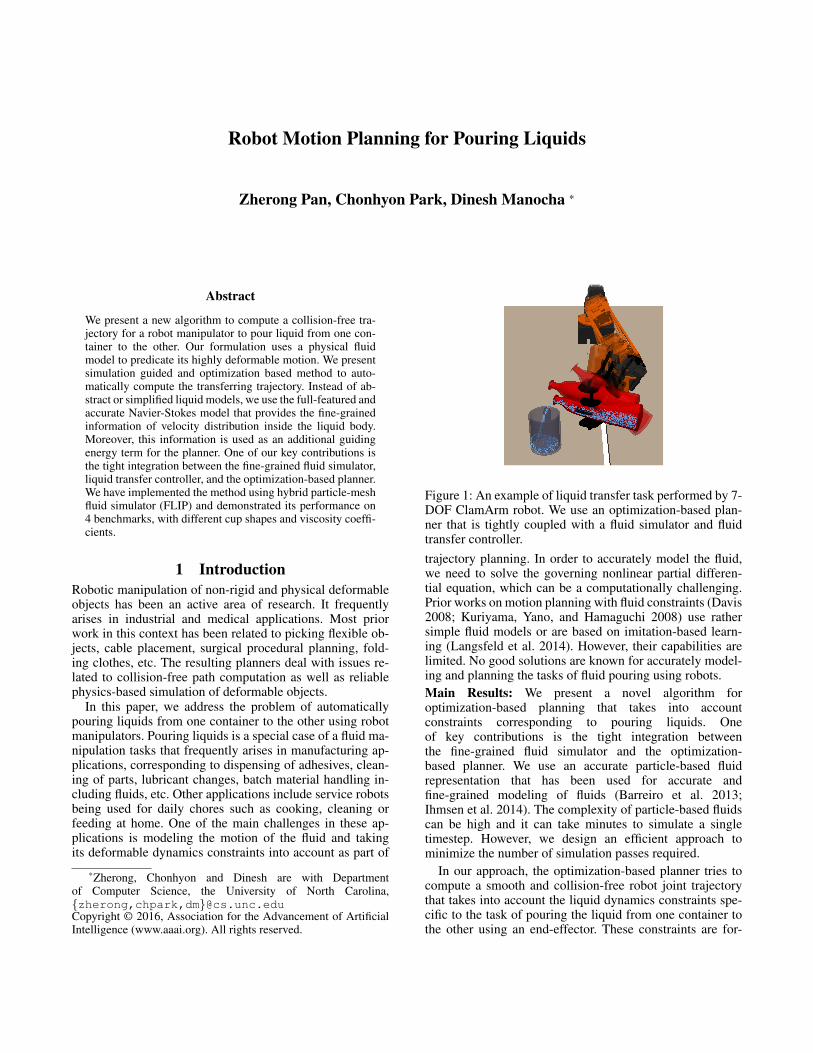
3.3 The Algorithm OverviewOur planning approach is illustrated in figure 3. The methodfirst tries to find an initial guess QC . It then iteratively findsa heuristic approximation c∗fluid to cfluid and computes newQC by optimizing:

E∗(QC) = cobs(Q

C) + csmooth(Q

C) + c∗fluid(Q

C),

until the function converges or reports failure after a fixednumber of iterations. In the next section, we refine the detailsof how cfluid, c

∗

fluid are defined.

4 Planning with Fluid ConstraintsIn this section, we present our planning algorithm that takesinto account the fluid dynamics constraints. Our formulationis based on using an energy formulation, cfluid(●,S(●)),and computing its approximation c∗fluid(●) to accelerate thecomputations. Finally, we combine it with our optimizationapproach to compute a trajectory for the end effector and themanipulator.

Liquid Transfer Controller

Liquid Analyser

Liquid Simulator

Optimization-BasedMotion Planner

QCk−1 c∗fluid E∗ QCk

cfluid

QC1,2

Figure 3: Overview of the various components of our motionplanning algorithm for pouring liquids. The symbols used inthis figures are the same as those used in algorithm 1.

4.1 Trajectory Initialization

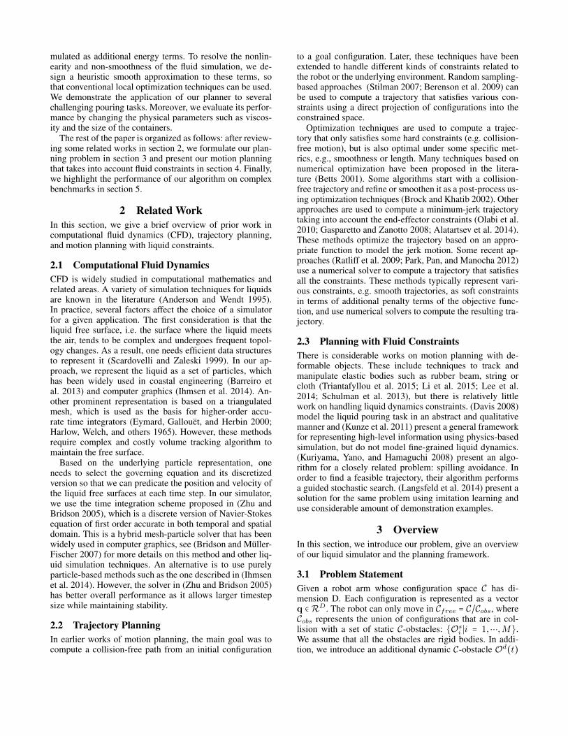
cOs0

cOd

Figure 8: The localcoordinate system andthe center of the openingfor source/target con-tainer, used to definethe objective functionequation 2.

The optimization algorithmneeds a good initial trajec-tory and refines it iterativelyin the high-dimensionalconfiguration space. Thisboils down to computingan initial trajectory QC

from the initial pose q1

following some qualitativeobservations of humanmanipulators. These ob-servations are integratedinto cfluid and the initialtrajectory is computed byoptimizing equation 1.First, for each of container Os

0,Od, we perform a simple

shape analysis to extract the center point of the openingon top of the container cOs

0,cOd attached with a frame,

as illustrated in figure 8. We perform this computation byusing a watershed algorithm (Roerdink and Meijster 2000)on the voxelized container to extract the opening and thencompute the centroid. We assume that Z = (0 0 1)

T is thenegative gravity direction.

We divide the pouring task into two phases: the movingphase P1 where robot orients Od properly to let liquid pourout; and then the pouring phase P2, where the robot triesto avoid spilling by making small perturbations to the ori-entation of Od. The time periods of these two phases aregiven as input parameters to the algorithm. We assume q1∼P

belongs to P1 and qP+1∼N belongs to P2. During P1, therobot moves cOd close to cOs

0as well as gradually turns Od

by an angle, e.g. 90○, along a horizontal axis. We formulatethis as an energy term:

corientfluid (qP ) = ∥ (ZT 0)TOd(qP ) (Z0

) ∥2.

Note that we only apply the orientation constraint totimestep P so that robot won’t move after timestep P sincethe term csmooth discourages any movement. In addition, wewant the opening of Od to be always pointing at cOs

0. This

observation introduces an additional term:

cdirfluid(qi) = ∥((cOs0− TOd(qi)cOd) ×

2(TOd(qi) (

Z0

))∥2,

where a ×2 b is the 2D cross product of the first 2 × 1 sub-vectors of a, b. We introduce no additional energy terms forP2. So that to get the initial trajectory, we use the followingcfluid:

cfluid(QC) = corientfluid (qP ) +Σi=1∼P cdirfluid(qi) + c

hintfluid, (2)

where the last term is a hint to guide the optimizer acrosshighly non-linear regions:

chintfluid(QC) = w∥cOs

0− TOd(qP )cOd∥

2,

which requires that the two opening centers are as close aspossible. We set w = 1E3 to guide the optimizer in a firstpass of optimization. And then we reduce w to 0.1 as a reg-ularization and run a second optimization. An example ofthe initial trajectory computed using our algorithm is shownin figure 9.

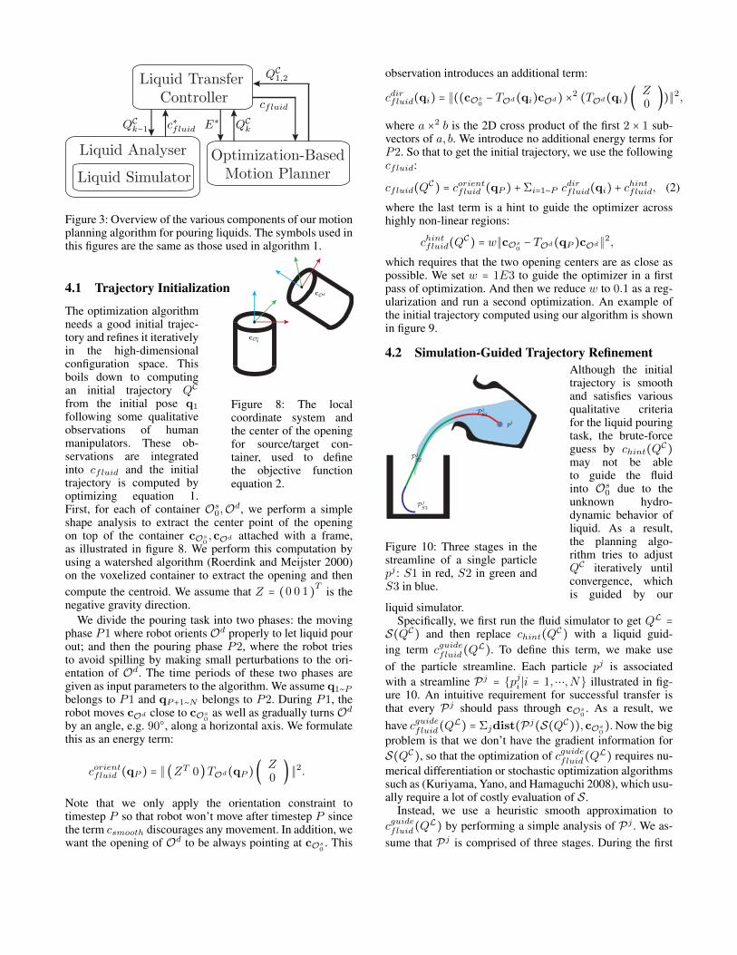
4.2 Simulation-Guided Trajectory Refinement

pj

PjS1

PjS2

PjS3

Figure 10: Three stages in thestreamline of a single particlepj : S1 in red, S2 in green andS3 in blue.

Although the initialtrajectory is smoothand satisfies variousqualitative criteriafor the liquid pouringtask, the brute-forceguess by chint(Q

C)

may not be ableto guide the fluidinto Os

0 due to theunknown hydro-dynamic behavior ofliquid. As a result,the planning algo-rithm tries to adjustQC iteratively untilconvergence, whichis guided by our

liquid simulator.Specifically, we first run the fluid simulator to get QL =

S(QC) and then replace chint(QC) with a liquid guid-

ing term cguidefluid(QL). To define this term, we make use

of the particle streamline. Each particle pj is associatedwith a streamline Pj

= {pji ∣i = 1,⋯,N} illustrated in fig-ure 10. An intuitive requirement for successful transfer isthat every Pj should pass through cOs

0. As a result, we

have cguidefluid(QL) = Σjdist(P

j(S(QC)),cOs

0). Now the big

problem is that we don’t have the gradient information forS(QC), so that the optimization of cguidefluid(Q

L) requires nu-

merical differentiation or stochastic optimization algorithmssuch as (Kuriyama, Yano, and Hamaguchi 2008), which usu-ally require a lot of costly evaluation of S .

Instead, we use a heuristic smooth approximation tocguidefluid(Q

L) by performing a simple analysis of Pj . We as-

sume that Pj is comprised of three stages. During the first

QC2 , i = 860 QC2 , i = 930 QC2 , i = 1060 QC2 , i = 1230

QC3 , i = 860 QC3 , i = 930 QC3 , i = 1060 QC3 , i = 1230

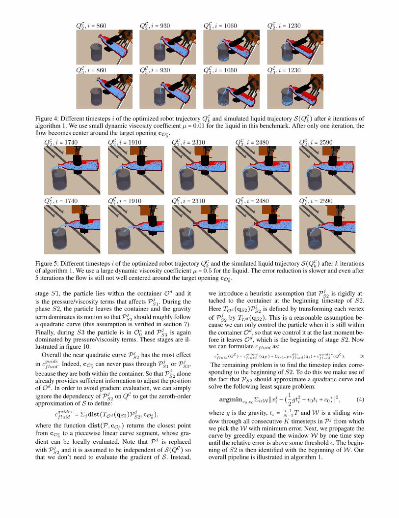
Figure 4: Different timesteps i of the optimized robot trajectory QCk and simulated liquid trajectory S(QCk) after k iterations ofalgorithm 1. We use small dynamic viscosity coefficient µ = 0.01 for the liquid in this benchmark. After only one iteration, theflow becomes center around the target opening cOs

0.

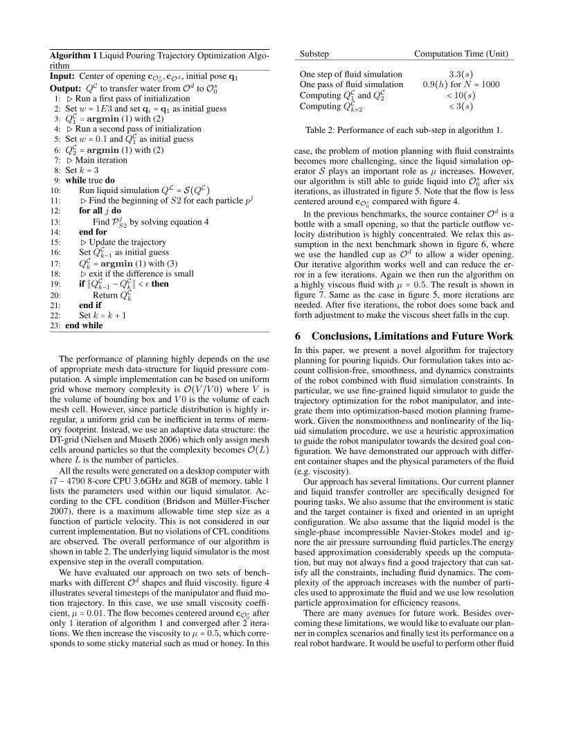
QC2 , i = 1740 QC2 , i = 1910 QC2 , i = 2310 QC2 , i = 2480 QC2 , i = 2590

QC7 , i = 1740 QC7 , i = 1910 QC7 , i = 2310 QC7 , i = 2480 QC7 , i = 2590

Figure 5: Different timesteps i of the optimized robot trajectory QCk and the simulated liquid trajectory S(QCk) after k iterationsof algorithm 1. We use a large dynamic viscosity coefficient µ = 0.5 for the liquid. The error reduction is slower and even after5 iterations the flow is still not well centered around the target opening cOs

0.

stage S1, the particle lies within the container Od and itis the pressure/viscosity terms that affects Pj

S1. During thephase S2, the particle leaves the container and the gravityterm dominates its motion so thatPj

S2 should roughly followa quadratic curve (this assumption is verified in section 7).Finally, during S3 the particle is in Os

0 and PjS3 is again

dominated by pressure/viscosity terms. These stages are il-lustrated in figure 10.

Overall the near quadratic curve PjS2 has the most effect

in cguidefluid . Indeed, cOs0

can never pass through PjS1 or Pj

S3,because they are both within the container. So thatPj

S2 alonealready provides sufficient information to adjust the positionof Od. In order to avoid gradient evaluation, we can simplyignore the dependency of Pj

S2 on QC to get the zeroth-orderapproximation of S to define:

cguide∗fluid = Σjdist(TOd(qS2)PjS2,cOs

0),

where the function dist(P,cOs0) returns the closest point

from cOs0

to a piecewise linear curve segment, whose gra-dient can be locally evaluated. Note that Pj is replacedwith Pj

S2 and it is assumed to be independent of S(QC) sothat we don’t need to evaluate the gradient of S. Instead,

we introduce a heuristic assumption that PjS2 is rigidly at-

tached to the container at the beginning timestep of S2.Here TOd(qS2)P

jS2 is defined by transforming each vertex

of PjS2 by TOd(qS2). This is a reasonable assumption be-

cause we can only control the particle when it is still withinthe containerOd, so that we control it at the last moment be-fore it leaves Od, which is the beginning of stage S2. Nowwe can formulate cfluid as:

c∗

fluid(QC) = c

orientfluid (qP ) +Σi=1∼P c

dirfluid(qi) + c

guide∗fluid

(QC). (3)

The remaining problem is to find the timestep index corre-sponding to the beginning of S2. To do this we make use ofthe fact that PS2 should approximate a quadratic curve andsolve the following least square problem:

argminv0,c0Σi∈W∥xji − (

1

2gt2i + v0ti + c0)∥

2, (4)

where g is the gravity, ti = i−1N−1

T and W is a sliding win-dow through all consecutive K timesteps in Pj from whichwe pick theW with minimum error. Next, we propagate thecurve by greedily expand the window W by one time stepuntil the relative error is above some threshold ε. The begin-ning of S2 is then identified with the beginning of W . Ouroverall pipeline is illustrated in algorithm 1.

QC2 , i = 780 QC2 , i = 910 QC2 , i = 1080 QC2 , i = 1340

QC3 , i = 780 QC3 , i = 910 QC3 , i = 1080 QC3 , i = 1340

Figure 6: Different timesteps i of the optimized robot trajectory QCk and simulated liquid trajectory S(QCk) after k iterations ofalgorithm 1. We use small dynamic viscosity coefficient µ = 0.01 for this liquid. Again, the flow is centered around the targetopening cOs

0but there is some splash at the beginning i = 780 which cannot be reduced by further iterations.

QC2 , i = 1740 QC2 , i = 1950 QC2 , i = 2330 QC2 , i = 2500 QC2 , i = 2640

QC6 , i = 1740 QC6 , i = 1950 QC6 , i = 2330 QC6 , i = 2500 QC6 , i = 2640

Figure 7: Different timesteps i of the optimized robot trajectory QCk and the simulated liquid trajectory S(QCk) after k iterationsof algorithm 1. We use a large dynamic viscosity coefficient µ = 0.5 for the liquid. Same as the case with figure 5, errorreduction is slower. After 4 iterations, robot moves Od back and forth, trying to make the viscous liquid fall inside Os

0.

Figure 9: An example of the initial trajectory for the bench-mark of figure 4 at timestep i = 250/1000,700/1000, whichis found using our two-stage algorithm.

5 Implementation and ResultsIn this section, we present the implementation details andhighlight the performance of our trajectory planning algo-rithm on challenging benchmarks. We use ROS (Quigleyet al. ) with 7-DOF ClamArm as the underlying manipula-tor. All the optimization computations are performed usingthe Augmented Lagrangian algorithm, with L-BFGS algo-rithm as the sub-problem solver. In terms of fluid dynamics,

Parameter Value (Unit)

Avg. Particle Radius 0.0075(m)

Gravity −9.81Z(m/s)∆t = T /N 0.01(s)No. Particles (Long Bottle) 60000No. Particles (Cup with Handle) 56000T 15(s)TP1 6(s)

Table 1: Parameters used in our liquid simulator: Averageparticle radius, gravity, time step size, number of particlesneed to fill the long bottle, number of particles to fill the cupwith handle, total sequence duration, duration of P1.

our implementation follows the outline of (Zhu and Bridson2005) combined with (Batty, Bertails, and Bridson 2007) forboundary handling. We precompute a signed distance fieldfor both Od and Os

0 as the solid boundaries, and we assumethat there is no collision between the robot and liquid parti-cles.

Algorithm 1 Liquid Pouring Trajectory Optimization Algo-rithmInput: Center of opening cOs

0,cOd , initial pose q1

Output: QC to transfer water from Od to Os0

1: ▷ Run a first pass of initialization2: Set w = 1E3 and set qi = q1 as initial guess3: QC1 = argmin (1) with (2)4: ▷ Run a second pass of initialization5: Set w = 0.1 and QC1 as initial guess6: QC2 = argmin (1) with (2)7: ▷ Main iteration8: Set k = 39: while true do

10: Run liquid simulation QL = S(QC)11: ▷ Find the beginning of S2 for each particle pj12: for all j do13: Find Pj

S2 by solving equation 414: end for15: ▷ Update the trajectory16: Set QCk−1 as initial guess17: QCk = argmin (1) with (3)18: ▷ exit if the difference is small19: if ∥QCk−1 −Q

C

k∥ < ε then20: Return QCk21: end if22: Set k = k + 123: end while

The performance of planning highly depends on the useof appropriate mesh data-structure for liquid pressure com-putation. A simple implementation can be based on uniformgrid whose memory complexity is O(V /V 0) where V isthe volume of bounding box and V 0 is the volume of eachmesh cell. However, since particle distribution is highly ir-regular, a uniform grid can be inefficient in terms of mem-ory footprint. Instead, we use an adaptive data structure: theDT-grid (Nielsen and Museth 2006) which only assign meshcells around particles so that the complexity becomes O(L)where L is the number of particles.

All the results were generated on a desktop computer withi7 − 4790 8-core CPU 3.6GHz and 8GB of memory. table 1lists the parameters used within our liquid simulator. Ac-cording to the CFL condition (Bridson and Muller-Fischer2007), there is a maximum allowable time step size as afunction of particle velocity. This is not considered in ourcurrent implementation. But no violations of CFL conditionsare observed. The overall performance of our algorithm isshown in table 2. The underlying liquid simulator is the mostexpensive step in the overall computation.

We have evaluated our approach on two sets of bench-marks with different Od shapes and fluid viscosity. figure 4illustrates several timesteps of the manipulator and fluid mo-tion trajectory. In this case, we use small viscosity coeffi-cient, µ = 0.01. The flow becomes centered around cOs

0after

only 1 iteration of algorithm 1 and converged after 2 itera-tions. We then increase the viscosity to µ = 0.5, which corre-sponds to some sticky material such as mud or honey. In this

Substep Computation Time (Unit)

One step of fluid simulation 3.3(s)One pass of fluid simulation 0.9(h) for N = 1000Computing QC1 and QC2 < 10(s)Computing QCk>2 < 3(s)

Table 2: Performance of each sub-step in algorithm 1.

case, the problem of motion planning with fluid constraintsbecomes more challenging, since the liquid simulation op-erator S plays an important role as µ increases. However,our algorithm is still able to guide liquid into Os

0 after sixiterations, as illustrated in figure 5. Note that the flow is lesscentered around cOs

0compared with figure 4.

In the previous benchmarks, the source container Od is abottle with a small opening, so that the particle outflow ve-locity distribution is highly concentrated. We relax this as-sumption in the next benchmark shown in figure 6, wherewe use the handled cup as Od to allow a wider opening.Our iterative algorithm works well and can reduce the er-ror in a few iterations. Again we then run the algorithm ona highly viscous fluid with µ = 0.5. The result is shown infigure 7. Same as the case in figure 5, more iterations areneeded. After five iterations, the robot does some back andforth adjustment to make the viscous sheet falls in the cup.

6 Conclusions, Limitations and Future WorkIn this paper, we present a novel algorithm for trajectoryplanning for pouring liquids. Our formulation takes into ac-count collision-free, smoothness, and dynamics constraintsof the robot combined with fluid simulation constraints. Inparticular, we use fine-grained liquid simulator to guide thetrajectory optimization for the robot manipulator, and inte-grate them into optimization-based motion planning frame-work. Given the nonsmoothness and nonlinearity of the liq-uid simulation procedure, we use a heuristic approximationto guide the robot manipulator towards the desired goal con-figuration. We have demonstrated our approach with differ-ent container shapes and the physical parameters of the fluid(e.g. viscosity).

Our approach has several limitations. Our current plannerand liquid transfer controller are specifically designed forpouring tasks. We also assume that the environment is staticand the target container is fixed and oriented in an uprightconfiguration. We also assume that the liquid model is thesingle-phase incompressible Navier-Stokes model and ig-nore the air pressure surrounding fluid particles.The energybased approximation considerably speeds up the computa-tion, but may not always find a good trajectory that can sat-isfy all the constraints, including fluid dynamics. The com-plexity of the approach increases with the number of parti-cles used to approximate the fluid and we use low resolutionparticle approximation for efficiency reasons.

There are many avenues for future work. Besides over-coming these limitations, we would like to evaluate our plan-ner in complex scenarios and finally test its performance on areal robot hardware. It would be useful to perform other fluid

manipulation tasks and design appropriate motion planningstrategies. We would like to accelerate the computations us-ing parallel algorithms that exploit multi-core CPUs andmany-core GPUs.

7 Appendix: Liquid SimulatorThe liquid simulator S used in our planner proceeds by re-peatedly applying the time integrator: pi+1 = f(qi,pi). Thegoverning equation of our solver is the single-phase incom-pressible Navier-Stokes equation:

Du

Dt= µ∇ ⋅ (∇u +∇uT ) + g −∇p

∇ ⋅ u = 0, (5)

where u is the velocity field inside the liquid body. On theright hand side are three body force terms that drive the liq-uid particles: the isotropic viscosity force with coefficient µ,the gravity force g, and the pressure force p. The dynamicviscosity coefficient µ describes how sticky the liquid is.For example, oil and honey have a larger µ as comparedwith water. Moreover, we introduce additional constraints∇ ⋅ u = 0, which essentially imply that the volume of fluid isconserved, so that the unknown pressure can be identified asthe Lagrangian multiplier and the resulting system is closed.

There are many ways to discretize equation 5, our simu-lator is based on (Zhu and Bridson 2005), and it is describedin algorithm 2. This is essentially a time-splitting integratorthat accounts for each of the three terms separately. In thisformulation, ∇⋅(∇u+∇uT )(x), is the evaluation of the dif-ferential operator ∇ ⋅ (∇u + ∇uT ) at x and ∇ ⋅ u(x) is theevaluation of∇⋅u at x. In order to perform these evaluations,we use a background grid and a finite difference scheme.These two terms require solving a globally coupled linearsystem and that becomes the computational bottleneck ofthe resulted simulator. For more details, we refer the readersto (Bridson and Muller-Fischer 2007).

Algorithm 2 The time integrator pi+1 = f(qi,pi)

Input: All particle pji ’s position xji and velocity ujiOutput: New positions xji+1 and velocities uji+1

1: ▷ Apply gravity force2: for all j do3: uj∗i = uji + g∆t4: end for5: ▷ Apply viscosity force6: for all j do7: (uj∗∗i − uj∗i ) = ∆tµ∇ ⋅ (∇u∗∗ +∇u∗∗T )(xji )8: end for9: ▷ Apply pressure force

10: for all j do11: (uji+1 − u

j∗∗i ) = −∆t∇pj , ∇ ⋅ u(xji ) = 0

12: end for13: ▷ Particle position update14: for all j do15: xji+1 = x

ji + u

ji+1∆t

16: end for

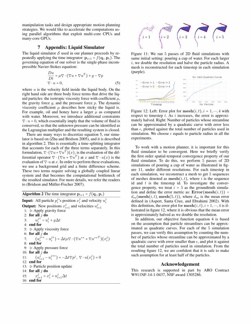
i = 1 i = 2 i = 3 i = 4 i = 5

Figure 11: We ran 5 passes of 2D fluid simulations withsame initial setting: pouring a cup of water. For each largeri, we double the resolution and halve the particle radius. Amesh is reconstructed for each timestep in each simulation(purple).

0

0.1

0.2

0.3

0.4

0.5

0.6

1

14

27

40

53

66

79

92

105

118

131

144

157

170

183

196

209

222

235

248

261

Timestep

Error i=1 Error i=2

Error i=3 Error i=4

0

5000

10000

15000

20000

25000

0 10000 20000 30000 40000 50000 60000

No. Particles

No. Valid Quadratic Curves

Figure 12: Left: Error plot for mesh(i, t), i = 1,⋯,4 withrespect to timestep t. As i increases, the error is approxi-mately halved. Right: Number of particles whose streamlinecan be approximated by a quadratic curve with error lessthan ε, plotted against the total number of particles used insimulation. We choose ε equals to particle radius in all theexperiments.

To work with a motion planner, it is important for thisfluid simulator to be convergent. Here we briefly verifythe first order spatial-temporal convergence property of ourfluid simulator. To do this, we perform 5 passes of 2Dsimulations of pouring a cup of water as illustrated in fig-ure 11, under different resolutions. For each timestep ineach simulation, we reconstruct a mesh to get 5 sequencesof meshes denoted as mesh(i, t), where i is the sequenceid and t is the timestep id. To investigate the conver-gence property, we treat i = 5 as the groundtruth simula-tion and define the error metric as: Error(mesh(i, t)) =

dm(mesh(i, t),mesh(5, t)), where dm is the mean errordefined in (Aspert, Santa Cruz, and Ebrahimi 2002). Withthis definition, the error plot for mesh(i, t), i = 1,⋯,4 is il-lustrated in figure 12, where it is obvious that the mean erroris approximately halved as we double the resolution.

In addition, our objective function equation 4 is basedon the assumption that particle streamlines can be approx-imated as quadratic curves. For each of the 5 simulationpasses, we can verify this assumption by counting the num-ber of particles whose streamline can be approximated by aquadratic curve with error smaller than ε, and plot it againstthe total number of particles used in simulation. From theresulting figure 12, we are confident that it is safe to makesuch assumption for at least half of the particles.

AcknowledgementThis research is supported in part by ARO ContractW911NF-14-1-0437, NSF award 1305286.

ReferencesAlatartsev, S.; Belov, A.; Nykolaichuk, M.; and Ortmeier, F.2014. Robot Trajectory Optimization for the Relaxed End-Effector Path. In Proceedings of the 11th International Con-ference on Informatics in Control, Automation and Robotics(ICINCO).Anderson, J. D., and Wendt, J. 1995. Computational fluiddynamics, volume 206. Springer.Aspert, N.; Santa Cruz, D.; and Ebrahimi, T. 2002. Mesh:measuring errors between surfaces using the hausdorff dis-tance. In ICME (1), 705–708.Barreiro, A.; Crespo, A.; Domınguez, J.; and Gomez-Gesteira, M. 2013. Smoothed particle hydrodynamicsfor coastal engineering problems. Computers & Structures120:96–106.Batty, C.; Bertails, F.; and Bridson, R. 2007. A fast varia-tional framework for accurate solid-fluid coupling. In ACMTransactions on Graphics (TOG), volume 26, 100. ACM.Berenson, D.; Srinivasa, S. S.; Ferguson, D.; Collet, A.; andKuffner, J. J. 2009. Manipulation planning with workspacegoal regions. In Proceedings of IEEE International Confer-ence on Robotics and Automation, 618–624.Betts, J. T. 2001. Practical methods for optimal control andestimation using nonlinear programming. In Advances indesign and control, volume 3. Siam.Bridson, R., and Muller-Fischer, M. 2007. Fluid simulation:Siggraph 2007 course notes video files associated with thiscourse are available from the citation page. In ACM SIG-GRAPH 2007 courses, 1–81. ACM.Brock, O., and Khatib, O. 2002. Elastic strips: A frameworkfor motion generation in human environments. InternationalJournal of Robotics Research 21(12):1031–1052.Davis, E. 2008. Pouring liquids: A study in commonsensephysical reasoning. Artificial Intelligence 172(12):1540–1578.Eymard, R.; Gallouet, T.; and Herbin, R. 2000. Finite vol-ume methods. Handbook of numerical analysis 7:713–1018.Gasparetto, A., and Zanotto, V. 2008. A technique for time-jerk optimal planning of robot trajectories. Robotics andComputer-Integrated Manufacturing 24(3):415–426.Harlow, F. H.; Welch, J. E.; et al. 1965. Numerical calcula-tion of time-dependent viscous incompressible flow of fluidwith free surface. Physics of fluids 8(12):2182.Ihmsen, M.; Orthmann, J.; Solenthaler, B.; Kolb, A.; andTeschner, M. 2014. Sph fluids in computer graphics.Kalakrishnan, M.; Chitta, S.; Theodorou, E.; Pastor, P.; andSchaal, S. 2011. STOMP: Stochastic trajectory optimizationfor motion planning. In Proceedings of IEEE InternationalConference on Robotics and Automation, 4569–4574.Kunze, L.; Dolha, M. E.; Guzman, E.; and Beetz, M. 2011.Simulation-based temporal projection of everyday robot ob-ject manipulation. In The 10th International Conference onAutonomous Agents and Multiagent Systems-Volume 1, 107–114. International Foundation for Autonomous Agents andMultiagent Systems.

Kuriyama, Y.; Yano, K.; and Hamaguchi, M. 2008. Tra-jectory planning for meal assist robot considering spillingavoidance. In Control Applications, 2008. CCA 2008. IEEEInternational Conference on, 1220–1225. IEEE.Langsfeld, J. D.; Kaipa, K. N.; Gentili, R. J.; Reggia, J. A.;and Gupta, S. K. 2014. Incorporating failure-to-successtransitions in imitation learning for a dynamic pouring task.Lee, A. X.; Huang, S. H.; Hadfield-Menell, D.; Tzeng, E.;and Abbeel, P. 2014. Unifying scene registration and tra-jectory optimization for learning from demonstrations withapplication to manipulation of deformable objects. In In-telligent Robots and Systems (IROS 2014), 2014 IEEE/RSJInternational Conference on, 4402–4407. IEEE.Li, Y.; Yue, Y.; Xu, D.; Grinspun, E.; and Allen, P. K.2015. Folding deformable objects using predictive simula-tion and trajectory optimization. In Proceedings of the 27thIEEE/RSJ International Conference on Intelligent Robotsand Systems (IROS).Nielsen, M. B., and Museth, K. 2006. Dynamic tubular grid:An efficient data structure and algorithms for high resolutionlevel sets. Journal of Scientific Computing 26(3):261–299.Olabi, A.; Bearee, R.; Gibaru, O.; and Damak, M. 2010.Feedrate planning for machining with industrial six-axisrobots. Control Engineering Practice 18(5):471–482.Park, C.; Pan, J.; and Manocha, D. 2012. ITOMP: In-cremental trajectory optimization for real-time replanningin dynamic environments. In Proceedings of InternationalConference on Automated Planning and Scheduling.Quigley, M.; Faust, J.; Foote, T.; and Leibs, J. Ros: an open-source robot operating system.Ratliff, N.; Zucker, M.; Bagnell, J. A. D.; and Srinivasa, S.2009. CHOMP: Gradient optimization techniques for effi-cient motion planning. In Proceedings of International Con-ference on Robotics and Automation, 489–494.Roerdink, J. B., and Meijster, A. 2000. The watershed trans-form: Definitions, algorithms and parallelization strategies.Scardovelli, R., and Zaleski, S. 1999. Direct numerical sim-ulation of free-surface and interfacial flow. Annual review offluid mechanics 31(1):567–603.Schulman, J.; Lee, A.; Ho, J.; and Abbeel, P. 2013. Trackingdeformable objects with point clouds. In Robotics and Au-tomation (ICRA), 2013 IEEE International Conference on,1130–1137. IEEE.Stilman, M. 2007. Task constrained motion planning inrobot joint space. In IEEE/RSJ International Conference onIntelligent Robots and Systems, 3074–3081.Triantafyllou, D.; Mariolis, I.; Kargakos, A.; Malassiotis, S.;and Aspragathos, N. 2015. A geometric approach to roboticunfolding of garments. Robotics and Autonomous Systems.Zhu, Y., and Bridson, R. 2005. Animating sand as a fluid.ACM Transactions on Graphics (TOG) 24(3):965–972.