Embed Size (px)
Citation preview

General rights Copyright and moral rights for the publications made accessible in the public portal are retained by the authors and/or other copyright owners and it is a condition of accessing publications that users recognise and abide by the legal requirements associated with these rights.
Users may download and print one copy of any publication from the public portal for the purpose of private study or research.
You may not further distribute the material or use it for any profit-making activity or commercial gain
You may freely distribute the URL identifying the publication in the public portal If you believe that this document breaches copyright please contact us providing details, and we will remove access to the work immediately and investigate your claim.
Downloaded from orbit.dtu.dk on: Mar 25, 2022
Robust long-term production planning
Muller, Laurent Flindt
Publication date:2011
Document VersionPublisher's PDF, also known as Version of record
Link back to DTU Orbit
Citation (APA):Muller, L. F. (2011). Robust long-term production planning. Technical University of Denmark.

Ph.D. thesis
Scheduling and Production
Planning Problems
Laurent Flindt Muller
Department of Management EngineeringTechnical University of Denmark,Produktionstorvet, Building 426,DK-2800 Kgs. Lyngby, Denmark
March, 2011

ii

Preface
The Ph.D. project was begun on the 1. of April 2008 at the Department of Computer Science atUniversity of Copenhagen (DIKU). After a year, the project moved to the Department of Man-agement Engineering at the Technical University of Denmark (DTU), because the main supervisorchanged his employment from DIKU to DTU.
When the project begun at DIKU, it was in cooperation with Microsoft, who financed partof the project. I would like to thank Microsoft for their involvement and the many interestingdiscussion we had during the first part of the project.
During the course of the project, I visited Professor Alper Atamturk at the Department ofIndustrial Engineering and Operations Research, at the University of California, Berkeley, and Iwould like to thank him, and the remaining staff and students, for their hospitality and fruitfuldiscussions.
I would also like to thank my two supervisors, David Pisinger (main supervisor), and MartinZachariasen (co-supervisor), for always taking the time to guide, help, and encourage me wheneverit was necessary.
Finally I would like to thank all my great colleagues at the Department of Management Engi-neering for many, many, many discussions.
iii

Preface iv

Contents
1 Introduction 11.1 Scheduling and production planning problems . . . . . . . . . . . . . . . . . . . . . 2
1.1.1 Disjunctive scheduling problems . . . . . . . . . . . . . . . . . . . . . . . . 21.1.2 Cumulative scheduling problems . . . . . . . . . . . . . . . . . . . . . . . . 31.1.3 Production planning problems . . . . . . . . . . . . . . . . . . . . . . . . . 5
1.2 Stochasticity . . . . . . . . . . . . . . . . . . . . . . . . . . . . . . . . . . . . . . . 61.2.1 Solution to a stochastic problem . . . . . . . . . . . . . . . . . . . . . . . . 71.2.2 Modelling a stochastic problem . . . . . . . . . . . . . . . . . . . . . . . . . 8
1.3 The Resource-Constrained Project Scheduling Problem . . . . . . . . . . . . . . . . 101.3.1 Formulations . . . . . . . . . . . . . . . . . . . . . . . . . . . . . . . . . . . 101.3.2 Bounds . . . . . . . . . . . . . . . . . . . . . . . . . . . . . . . . . . . . . . 131.3.3 Instances . . . . . . . . . . . . . . . . . . . . . . . . . . . . . . . . . . . . . 151.3.4 A brief overview of exact and heuristic solution methods . . . . . . . . . . . 151.3.5 Overview of a branch-and-cut method for the Multi-mode Resource-Con-
strained Project Scheduling Problem . . . . . . . . . . . . . . . . . . . . . . 161.4 Thesis outline . . . . . . . . . . . . . . . . . . . . . . . . . . . . . . . . . . . . . . . 17
2 An Adaptive Large Neighborhood Search Algorithm for the Resource-Constrai-ned Project Scheduling Problem 292.1 Introduction . . . . . . . . . . . . . . . . . . . . . . . . . . . . . . . . . . . . . . . . 292.2 Adaptive Large Neighborhood Search . . . . . . . . . . . . . . . . . . . . . . . . . 302.3 Algorithm . . . . . . . . . . . . . . . . . . . . . . . . . . . . . . . . . . . . . . . . . 302.4 Neighborhoods . . . . . . . . . . . . . . . . . . . . . . . . . . . . . . . . . . . . . . 332.5 Experiments . . . . . . . . . . . . . . . . . . . . . . . . . . . . . . . . . . . . . . . . 35
2.5.1 Effect of parameters . . . . . . . . . . . . . . . . . . . . . . . . . . . . . . . 362.5.2 Effect of SGS . . . . . . . . . . . . . . . . . . . . . . . . . . . . . . . . . . . 372.5.3 Effect of number of restarts . . . . . . . . . . . . . . . . . . . . . . . . . . . 372.5.4 Effect of components . . . . . . . . . . . . . . . . . . . . . . . . . . . . . . . 372.5.5 Effect of adaptive layer . . . . . . . . . . . . . . . . . . . . . . . . . . . . . 38
2.6 Computational results . . . . . . . . . . . . . . . . . . . . . . . . . . . . . . . . . . 382.7 Conclusion . . . . . . . . . . . . . . . . . . . . . . . . . . . . . . . . . . . . . . . . 39
3 An Adaptive Large Neighborhood Search Algorithm for the Multi-mode Re-source-Constrained Project Scheduling Problem 433.1 Introduction . . . . . . . . . . . . . . . . . . . . . . . . . . . . . . . . . . . . . . . . 433.2 Problem description . . . . . . . . . . . . . . . . . . . . . . . . . . . . . . . . . . . 453.3 Adaptive large neighborhood search . . . . . . . . . . . . . . . . . . . . . . . . . . 453.4 Lower bounds . . . . . . . . . . . . . . . . . . . . . . . . . . . . . . . . . . . . . . . 463.5 Algorithm . . . . . . . . . . . . . . . . . . . . . . . . . . . . . . . . . . . . . . . . . 48
v

Contents vi
3.6 Neighborhoods . . . . . . . . . . . . . . . . . . . . . . . . . . . . . . . . . . . . . . 54
3.7 Computational experiments . . . . . . . . . . . . . . . . . . . . . . . . . . . . . . . 56
3.7.1 Lower bounds . . . . . . . . . . . . . . . . . . . . . . . . . . . . . . . . . . . 57
3.7.2 Components . . . . . . . . . . . . . . . . . . . . . . . . . . . . . . . . . . . 59
3.7.3 Final results . . . . . . . . . . . . . . . . . . . . . . . . . . . . . . . . . . . 61
3.8 Conclusion . . . . . . . . . . . . . . . . . . . . . . . . . . . . . . . . . . . . . . . . 62
4 Separation and extension of cover inequalities for second-order conic knapsackconstraints with generalized upper bounds 69
4.1 Introduction . . . . . . . . . . . . . . . . . . . . . . . . . . . . . . . . . . . . . . . . 69
4.2 Cover inequalities . . . . . . . . . . . . . . . . . . . . . . . . . . . . . . . . . . . . . 71
4.2.1 Extended cover inequalities . . . . . . . . . . . . . . . . . . . . . . . . . . . 71
4.2.2 Extended cover inequalities with GUB constraints . . . . . . . . . . . . . . 71
4.3 Algorithms for extending cover inequalities . . . . . . . . . . . . . . . . . . . . . . 74
4.3.1 Optimal . . . . . . . . . . . . . . . . . . . . . . . . . . . . . . . . . . . . . . 74
4.3.2 Lower bound 1 . . . . . . . . . . . . . . . . . . . . . . . . . . . . . . . . . . 74
4.3.3 Lower bound 2 . . . . . . . . . . . . . . . . . . . . . . . . . . . . . . . . . . 75
4.4 Separation of cover inequalities . . . . . . . . . . . . . . . . . . . . . . . . . . . . . 76
4.4.1 Algorithms for separating base covers . . . . . . . . . . . . . . . . . . . . . 77
4.5 Computational experiments . . . . . . . . . . . . . . . . . . . . . . . . . . . . . . . 78
4.5.1 Test instances . . . . . . . . . . . . . . . . . . . . . . . . . . . . . . . . . . . 78
4.5.2 Test setup . . . . . . . . . . . . . . . . . . . . . . . . . . . . . . . . . . . . . 78
4.5.3 Cuts . . . . . . . . . . . . . . . . . . . . . . . . . . . . . . . . . . . . . . . . 79
4.5.4 Results . . . . . . . . . . . . . . . . . . . . . . . . . . . . . . . . . . . . . . 79
4.6 Conclusion . . . . . . . . . . . . . . . . . . . . . . . . . . . . . . . . . . . . . . . . 84
5 A Multi-mode Resource-Constrained Project Scheduling Problem with Sto-chastic Nonrenewable Resource Consumption 89
5.1 Introduction . . . . . . . . . . . . . . . . . . . . . . . . . . . . . . . . . . . . . . . . 89
5.2 Problem . . . . . . . . . . . . . . . . . . . . . . . . . . . . . . . . . . . . . . . . . . 91
5.3 Model . . . . . . . . . . . . . . . . . . . . . . . . . . . . . . . . . . . . . . . . . . . 92
5.3.1 Modelling chance constraints . . . . . . . . . . . . . . . . . . . . . . . . . . 92
5.3.2 Separating joint chance constraints . . . . . . . . . . . . . . . . . . . . . . . 92
5.3.3 Conic Quadratic Integer Program . . . . . . . . . . . . . . . . . . . . . . . . 92
5.4 Conic cover cuts . . . . . . . . . . . . . . . . . . . . . . . . . . . . . . . . . . . . . 93
5.5 Solution methodology . . . . . . . . . . . . . . . . . . . . . . . . . . . . . . . . . . 94
5.5.1 Finish-to-Start-Distance-matrix and lower bounds . . . . . . . . . . . . . . 95
5.5.2 Preprocessing . . . . . . . . . . . . . . . . . . . . . . . . . . . . . . . . . . . 96
5.5.3 Upper bounds and problem reductions . . . . . . . . . . . . . . . . . . . . . 96
5.5.4 Initial variable reduction . . . . . . . . . . . . . . . . . . . . . . . . . . . . . 98
5.5.5 Variables and branching . . . . . . . . . . . . . . . . . . . . . . . . . . . . . 98
5.5.6 Variables and propagation . . . . . . . . . . . . . . . . . . . . . . . . . . . . 99
5.5.7 Finish-to-Start-Distance (FSD)-matrix-based mode removal . . . . . . . . . 100
5.5.8 FSD-matrix-based pruning . . . . . . . . . . . . . . . . . . . . . . . . . . . 100
5.6 Computational experiments . . . . . . . . . . . . . . . . . . . . . . . . . . . . . . . 100
5.6.1 Benchmark instances . . . . . . . . . . . . . . . . . . . . . . . . . . . . . . . 101
5.6.2 Evaluation of components . . . . . . . . . . . . . . . . . . . . . . . . . . . . 101
5.6.3 Final results . . . . . . . . . . . . . . . . . . . . . . . . . . . . . . . . . . . 103
5.7 Conclusion . . . . . . . . . . . . . . . . . . . . . . . . . . . . . . . . . . . . . . . . 104

vii Contents
6 A solution approach to a stochastic large scale energy management problembased on Benders Decomposition 1096.1 Introduction . . . . . . . . . . . . . . . . . . . . . . . . . . . . . . . . . . . . . . . . 1096.2 Problem Definition . . . . . . . . . . . . . . . . . . . . . . . . . . . . . . . . . . . . 1116.3 Model . . . . . . . . . . . . . . . . . . . . . . . . . . . . . . . . . . . . . . . . . . . 1156.4 Methodology . . . . . . . . . . . . . . . . . . . . . . . . . . . . . . . . . . . . . . . 118
6.4.1 Benders Decomposition . . . . . . . . . . . . . . . . . . . . . . . . . . . . . 1186.4.2 Benders Reformulation . . . . . . . . . . . . . . . . . . . . . . . . . . . . . . 1196.4.3 Solution Approach . . . . . . . . . . . . . . . . . . . . . . . . . . . . . . . . 120
6.5 Reducing the problem size . . . . . . . . . . . . . . . . . . . . . . . . . . . . . . . . 1216.5.1 Preprocessing . . . . . . . . . . . . . . . . . . . . . . . . . . . . . . . . . . . 1216.5.2 Aggregation . . . . . . . . . . . . . . . . . . . . . . . . . . . . . . . . . . . . 123
6.6 Feasibility . . . . . . . . . . . . . . . . . . . . . . . . . . . . . . . . . . . . . . . . . 1256.6.1 Fuel bounding constraints . . . . . . . . . . . . . . . . . . . . . . . . . . . . 1256.6.2 Fuel cuts . . . . . . . . . . . . . . . . . . . . . . . . . . . . . . . . . . . . . 125
6.7 Postprocessing . . . . . . . . . . . . . . . . . . . . . . . . . . . . . . . . . . . . . . 1276.7.1 Repair . . . . . . . . . . . . . . . . . . . . . . . . . . . . . . . . . . . . . . . 1276.7.2 Postoptimization . . . . . . . . . . . . . . . . . . . . . . . . . . . . . . . . . 128
6.8 Computational results . . . . . . . . . . . . . . . . . . . . . . . . . . . . . . . . . . 1296.9 Conclusion . . . . . . . . . . . . . . . . . . . . . . . . . . . . . . . . . . . . . . . . 133
7 A hybrid Adaptive Large Neighborhood Search heuristic for lot-sizing withsetup times 1377.1 Introduction . . . . . . . . . . . . . . . . . . . . . . . . . . . . . . . . . . . . . . . . 1377.2 A hybrid ALNS algorithm . . . . . . . . . . . . . . . . . . . . . . . . . . . . . . . . 1397.3 An application of ALNS to the LSPST . . . . . . . . . . . . . . . . . . . . . . . . . 141
7.3.1 Problem description . . . . . . . . . . . . . . . . . . . . . . . . . . . . . . . 1417.3.2 Local search . . . . . . . . . . . . . . . . . . . . . . . . . . . . . . . . . . . . 1417.3.3 Adaptive weight adjustments . . . . . . . . . . . . . . . . . . . . . . . . . . 1427.3.4 Destroy neighborhoods . . . . . . . . . . . . . . . . . . . . . . . . . . . . . . 1427.3.5 Repair neighborhoods . . . . . . . . . . . . . . . . . . . . . . . . . . . . . . 1437.3.6 ALNS parameters . . . . . . . . . . . . . . . . . . . . . . . . . . . . . . . . 1437.3.7 Overview . . . . . . . . . . . . . . . . . . . . . . . . . . . . . . . . . . . . . 144
7.4 Experimental results . . . . . . . . . . . . . . . . . . . . . . . . . . . . . . . . . . . 1447.4.1 Instances . . . . . . . . . . . . . . . . . . . . . . . . . . . . . . . . . . . . . 1447.4.2 Comparison . . . . . . . . . . . . . . . . . . . . . . . . . . . . . . . . . . . . 145
7.5 Conclusion . . . . . . . . . . . . . . . . . . . . . . . . . . . . . . . . . . . . . . . . 1467.A Detailed results . . . . . . . . . . . . . . . . . . . . . . . . . . . . . . . . . . . . . . 147
8 Conclusion 1538.1 Summary, perspectives, and further research . . . . . . . . . . . . . . . . . . . . . . 1538.2 General thoughts . . . . . . . . . . . . . . . . . . . . . . . . . . . . . . . . . . . . . 1558.3 Final words . . . . . . . . . . . . . . . . . . . . . . . . . . . . . . . . . . . . . . . . 156

Contents viii

Chapter 1
Introduction
Scheduling and production planning is a field which has a wide area of application, and a historywhich dates back to the beginning of the industrial revolution. Still, researchers and commercialsoftware vendors are working on problems within this area, driven by the fact that cost savings ofa few percent, or improved customer satisfaction may be an important competitive factor. Addi-tionally in a time of austerity getting the best performance from existing resources is important.
From the literature it is not always clear what, if any, the distinction is between schedulingand production planning. We take the following view (a similar view of scheduling is taken byDemeulemeester and Herroelen (2002), and a similar view of production planning is taken byPochet and Wolsey (2006)):
Scheduling For scheduling problems the emphasis is on the duration aspect, and the entitiesunder consideration are activities (depending on the context they may also be known asoperations or jobs) having a certain duration. As an example, in the context of car productionan activity could be “Left door should be mounted on car” which take, say, 60 seconds, andin the context of software engineering it could be “Implement interface to database”, whichis estimated to take, say, 2 days. For the activities to be executed they require a certainamount of resources known in advance. In the context of the car production example thiscould be a worker and, say, a screwdriver, while in the context of the software engineeringexample this could be a programmer. The goal is to decide when activities start and stopsuch as to minimize some cost, which is a function of the completion times of the activities.
Production planning For production planning the emphasis is on satisfying demand for itemsat different points in time at minimum cost. For such problems one typically needs to decidehow many items to produce and when to do it, and there are typically costs associated withkeeping items on stock. In the context of car production an item could be “Red Peugeot306” while another could be “White Peugeot 405”, and by some knowledge we know we mustdeliver, say, 200 of the first item at some specific date, and 140 of the second item at someother specific date.
Production planning decisions are typically at a higher strategic level than scheduling decisions.Since scheduling and production planning covers a wide range of problems, there are also a largenumber of different models found in the literature. We will describe some of these in the nextsection. The models differ with respect to assumptions, and perspective: some models focus ondecisions at the strategic level, while other models focus on decisions at the tactical level, andother models again focus on decisions at the operational level. The primary focus of this thesiswill be the Resource-Constrained Project Scheduling Problem (RCPSP), which is a very generalscheduling model, containing many scheduling problems as special cases. It is primarily used tomodel decisions at the tactical and operational levels. The RCPSP itself exists in a number ofvariants, many of which lie close to models found in commercial software packages, and is thusnot only interesting from a theoretical point of view (it is NP-hard), but also form a practical
1

Chapter 1. Introduction 2
perspective. Two variants will be the main focus of this thesis, the so-called single-mode and multi-mode variants, both of which will be described in detail in Section 1.1. In addition to the RCPSPwe will also be considering a so-called lot-sizing problem, which is an example of a productionplanning problem. A description of such a lot-sizing problem will also be given in Section 1.1.Some of the problems considered will be of a stochastic nature, and we will in Section 1.2 discussstochasticity both in general, and in context of the RCPSP. As the main focus of the thesis isthe RCPSP we, in Section 1.3, discuss some background knowledge, which will be assumed inthe following chapters. Finally in Section 1.4 we give an outline of the remaining chapters of thisthesis.
1.1 Scheduling and production planning problems
In this section we give an overview of some scheduling and production planning problems found inthe literature, in order to better place the RCPSP within a context. When considering schedulingproblems, a distinction can be made between so-called disjunctive scheduling problems and so-called cumulative scheduling problems. In disjunctive scheduling problems a resource (dependingon context a resource may also be known as a machine) may only execute one activity at a time,while for cumulative scheduling problems many activities may be in progress simultaneously. Thuscumulative scheduling problems are more general than disjunctive scheduling problems. In thefollowing we treat these two kinds of scheduling problems separately.
1.1.1 Disjunctive scheduling problems
In the following we describe some disjunctive scheduling problems. Some of the symbols used forthe definitions will be the same but have slightly different meaning. Only the notation used fordefining the RCPSP will be used generally, for the remaining problems, it is only valid within theappropriate section.
The Job Shop Scheduling Problem
One well-known disjunctive scheduling problem is the Job Shop Scheduling Problem (JSSP) whichcan be described as follows: The problem consists of a set of jobs J = {1, . . . , n} and a set ofmachines M = {1, . . . ,m}. Each job j ∈ J must be processed exactly once on each machine.Each job defines an order in which it should be processed on the machines. For a job j ∈ J letπj(k), 1 ≤ k ≤ m, denote the kth machine for j. The processing of job j ∈ J on machine πj(k)is called an operation, and denoted ojk. An operation ojk has an duration of pjk and can not bepreempted, i.e., the processing of an operation can not be interrupted and then resumed at a laterpoint in time. For a machine k ∈M let ρk(j), 1 ≤ j ≤ J , be the index of the operation of j whichmust be processed on k. Each operation of a job must occur one after the other, i.e., operation ojkmay not be started before operation oj,k−1 has completed. Only one operation may be in progressat a time on each machine. Let σjk denote the starting time of operation ojk. The objective is tominimize the project makespan, i.e., the total time needed to complete all operations. The JSSPis NP-hard for |M | ≥ 2 and |J | ≥ 3 (see Garey et al. (1976)). The problem may be stated as thefollowing mathematical program:
min maxj∈J
σjm + pjm
s.t. σjk ≥ σj,k−1 + pj,k−1 ∀j ∈ J, k = 2, . . . ,m (1.1)
σjρk(j) ≥ σiρk(i) + piρk(i) ∨ σiρk(i) ≥ σjρk(j) + pjρk(j) ∀k ∈M, ∀i, j ∈ J (1.2)
σjk ≥ 0 ∀j ∈ J, ∀k ∈M (1.3)
Constraints (1.1) enforce the sequencing of the activities of a job, and Constraints (1.2) ensurethat operations running on the same machine are sequenced. Note that the constraints (1.2) arenot linear because of the disjunction.

3 1.1. Scheduling and production planning problems
Two popular variants are the Open Shop Scheduling Problem, and the Flow Shop Schedulingproblem. For the former problem, there are no sequencing constraints for the operations of a job,while for the latter problem the sequencing of machines is the same for each job.
The JSSP is from a modeling point of view very simple, yet general enough to model manyreal-life situations, such as a factory floor, where there is no choice of which machine to be usedfor a given operation, and each machine can only perform a single operation at a time. The maindifference between the JSSP and the other models considered here, is the lack of choice, and thedisjunctiveness.
The Multi-Skill Project Scheduling Problem
Another disjunctive scheduling problem is the Multi-Skill Project Scheduling Problem (MSPSP)(see Neron and Baptista (2002)). Here resources model staff members each having a set of skills,and activities requiring a certain set of skills in order to be executed. This problem is NP-hardand may be described as follows: A project consists of a set A = {1, . . . , n} of activities, a set ofresources, i.e., persons, R = {1, . . . , |R|}, and a set of skills L = {1, . . . , |L|}. Activity 1 and nare so-called dummy activities, which represent the start and the end of the project. Each personk ∈ R possesses some subset of skills, and each activity j ∈ A requires bjh persons with skillh ∈ L while in progress, has a processing time of pj , and can not be preempted. Let Qkh = 1 ifand only if person k has skill h and zero otherwise. There may exist precedence relations betweenactivities, such that one activity may not be started before some others have completed. LetE = {(i, j) ∈ A2 : i must precede j} be the set of all precedence relations. Each person mayonly perform one activity at a time. There may be points in time where certain persons are notavailable. Let Wt ⊆ R be the persons not available for work at time t. The aim is to find aschedule which satisfies all the constraints and which minimizes the project makespan across sometime horizon T of time steps. For a given solution, let σj be the starting time of activity j ∈ A,let R(j) ⊆ R the set of persons assigned to activity j, and let A(k) ⊆ A be the activities assignedto person k ∈ R. The problem may be stated as the following mathematical program:
min σn
s.t. σj ≥ σi + pi ∀(i, j) ∈ E , (1.4)
σj ≥ σi + pi ∨ σi ≥ σj + pj ∀k ∈ R, ∀i, j ∈ A(k) (1.5)∑
k∈R(j)
Qkh ≥ bjh ∀j ∈ A, ∀h ∈ L (1.6)
Wt ∩R(j) = ∅ ∀j ∈ A, t = σj , . . . , σj + pj (1.7)
σj ≥ 0 ∀j ∈ A, (1.8)
Constraints (1.4) enforce the precedence constraints, Constraints (1.5) ensure activities performedby a person are sequenced, Constraints (1.6) enforce that the skill requirements of activities aremet, and Constraints (1.7) enforce that persons do not work when they are not available.
The MSPSP is more general than the JSSP described earlier, as an activity may occupy morethan one resource at a time and there is a choice of which resources to occupy. The MSPSPwould typically be used in a setting, which is heavy on human labor, and where one has manyalternatives for performing an activity, such as the software engineering example given earlier.
1.1.2 Cumulative scheduling problems
We in the following describe some cumulative scheduling problems.
The Cumulative Scheduling Problem
A scheduling problem encountered in the literature is the Cumulative Scheduling Problem (CuSP)which is NP-hard (see Baptiste et al. (1999) and Carlier and Neron (2000)). The CuSP can be

Chapter 1. Introduction 4
described as follows: A set of activities A = {1, . . . , n} must be performed on a single resourcewhich has a constant capacity R. Each activity j ∈ A has a processing time pj (non-preemptive),and requires rj units of the resource while it is in progress. Each activity j ∈ A, is associated witha release time trj and due date tdj , and the activity must be performed in the interval [trj ; t
dj ]. Let
T be a set of time steps. The aim is to find a feasible schedule, which minimizes the makespan.Given a solution, let σj be the starting time of activity j ∈ A. The problem may be stated as thefollowing mathematical program:
min maxj∈A
σj + pj
s.t.∑
j∈A(t)
rj ≤ R ∀t ∈ T (1.9)
trj ≤ σj ≤ tdj − pj ∀j ∈ A (1.10)
σj ≥ 0 ∀j ∈ A, (1.11)
where A(t) = {j ∈ A|σj ≤ t ≤ σj + pj}, i.e., the activities in progress at time t ∈ T . Constraints(1.9) ensure that at no point in time is the capacity of the resource exceeded, and Constraints (1.10)ensure that an activity is processed with the interval defined by its release time and due date.
An interesting relaxation of the CuSP is the so-called fully elastic CuSP, which is solvablein polynomial time (see Baptiste et al. (1999)). Here rather than having a processing time andresource usage, each activity j ∈ A requires some amount of work, Wj , and the activity completeswhen this amount of work has been performed. That is one has the requirements
tdj∑
t=trj
wjt = Wj ∀j ∈ A,∑
j∈A
wjt ≤ R ∀t ∈ T
where wjt is the amount of work done for activity j in time step t. This relaxation is interestingbecause it allows for modeling trade-offs between the amount of resources consumed per time step,and the number of time steps an activity must be processed, which would be useful in in caseswhere the value Wj represents some flexible resource such as man-hours, which could be spreadin a number different ways across a time period.
The Resource-Constrained Project Scheduling Problem
A very widely studied cumulative scheduling problem found in the literature is the RCPSP. Thisproblem was first described by Pritsker et al. (1969) and as a generalization of the JSSP it isNP-hard (cf. Blazewicz et al. (1983)). There exists a number of variants of the RCPSP, seefor instance Blazewicz et al. (1983), Brucker et al. (1999), or Hartmann and Briskorn (2010).We now give a description of two of the most commonly encountered variants, that are also thebasis of variants considered in this thesis, namely the Single-mode Resource-Constrained ProjectScheduling Problem (SRCPSP) and the Multi-mode Resource-Constrained Project SchedulingProblem (MRCPSP). As the MRCPSP is a generalization of the SRCPSP, we define the multi-mode variant formally, and then describe the single-mode variant within the context of the multi-mode.
The MRCPSP can be described as follows (see for instance Talbot (1982) or Brucker et al.(1999)): A project consists of a set A = {1, . . . , n} of activities, to be scheduled. Activity 1 and nare so-called dummy activities, that represent the start and the end of the project. Each activityj can be performed in a number of different modes Mj = {1, . . . , |Mj |}, each representing analternative way of performing the activity. There are two sets of resources, (1) renewable resourcesR = {1, . . . , |R|}, and (2) nonrenewable resources R = {1, . . . , |R|}. A renewable resource k ∈ R,has capacity Rk in each time period, while a nonrenewable resource k ∈ R has capacity Rk. Whenan activity j is scheduled in mode m ∈ Mj, it has a processing time of pjm (non-preemptive)

5 1.1. Scheduling and production planning problems
and requires rjkm ≥ 0 units of renewable resource k ∈ R in each time period, and rjkm ≥ 0 of
nonrenewable resource k ∈ R across all time periods. There exists precedence relations betweenthe activities, such that one activity j ∈ A can not be started before all its predecessors, Pj , havecompleted. Symmetrically, Sj denotes the set of successors. Let E = {(i, j) ∈ A2 : i ∈ Pj} bethe set of all precedence relations. Given a solution, let σj be the starting time of activity j andlet m(j) ∈ Mj be the mode chosen for activity j. The problem may be stated as the followingmathematical program:
min σn
s.t. σj ≥ σi + pi,m(i) ∀(i, j) ∈ E (1.12)∑
j∈A(t)
rj,k,m(j) ≤ Rk ∀k ∈ R, ∀t ∈ T (1.13)
∑
j∈A
rj,k,m(j) ≤ Rk ∀k ∈ R (1.14)
σj ≥ 0 ∀j ∈ A, (1.15)
where A(t) = {j ∈ A|σj ≤ t ≤ σj + pj,m(j)}, i.e., the set of activities in progress at time t ∈ T .Constraints (1.12) enforce the precedence constraints, Constraints (1.13) ensure that at no pointin time do the activities in progress exceed the capacity of a resource, and Constraints (1.14)ensure that the capacity of the nonrenewable resources are not exceeded.
For the SRCPSP, there is only a single mode for each activity, and all resources are renewable,i.e.,Mj = {1} ∀j ∈ A, and R = ∅. When considering the SRCPSP we omit the subscript m.
The RCPSP is very flexible, and it can be used to model the JSSP, the CuSP, and the MSPSP,although the number of modes may be exponential in the case of the MSPSP.
1.1.3 Production planning problems
In this section we describe a general production planning problem. Such a problem is often referredto as a lot-sizing problem in the literature. There exists a large number of lot-sizing problems(see for instance Pochet and Wolsey (2006)). A generic lot-sizing problem could be the following:A number of items must be produced on a number of machines, such that varying demands forthese items are met across a time horizon at minimum cost. Each item has a unit production cost,and a unit holding cost per time step the item is kept on stock. Each machine has a limited itemcapacity and may produce more than an single item. Variants of the problem are numerous andmay include whether the machines have constant capacity or time-varying, whether lot-sizes arefixed or dynamic, whether a price is paid when switching from production of one item to another,the granularity of the time-steps, whether backlogging is allowed at a cost, whether items areinterdependent, and whether a machine can produce more than a single item in a time step.
One axis about which lot-sizing problems may be divided is that of big-bucket versus small-bucket models. In very general terms, the main difference between the two kinds of models, is thetime granularity of the problem. Typically for big-bucket models time steps represent long timespans, while they represent much shorter time spans for small-bucket models, and the small-bucketmodels are thus closer to the concept of scheduling.
In the following we give an example of one such lot-sizing problem.
Multi-item Capacitated Lot Sizing Problem with Setup Times
The Multi-item Capacitated Lot Sizing Problem with Setup Times (CLSP) is a big-bucket model.In a big-bucket model more than a single item may be produced per time step, and an item iscompleted in the same time step as the one where production is initiated (whereas in small-bucketmodels only a single item may be produced per time period, and items are completed after acertain number of time steps passes). The problem may be described as follows: Schedule the

Chapter 1. Introduction 6
production of a set of items, I = {1, . . . , n}, over a given number of time periods, T , such thatall demand dit of each items i ∈ I at time t ∈ T is met. The items must all be produced on thesame resource, such that its time-dependant capacity, Ct ≥ 0 for t ∈ T , is not exceeded. Theproduction of each unit of item i ∈ I at time t ∈ T uses αi
t ≥ 0 capacity on the resource, and has afixed capacity setup cost on the resource of βi
t ≥ 0 and a fixed setup cost of f it ≥ 0. Producing one
unit of item i ∈ I has a cost of pit ≥ 0 at time t ∈ T , and the holding cost for a unit of item i ∈ Ifrom time step t to the next is hi
t ≥ 0. The problem may be stated as the following mathematicalmodel:
min∑
i∈I
(
hi0s
i0 +
∑
t∈T
(hits
it + pitx
it + f i
tyit)
)
s.t. sit−1 + xit = dit + sit t ∈ T , i ∈ I (1.16)
xit ≤Myit t ∈ T , i ∈ I (1.17)∑
i∈I
(
αitx
it + βi
tyit
)
≤ Ct t ∈ T (1.18)
sit, s0t , x
it ≥ 0, yit ∈ {0, 1} t ∈ T , i ∈ I, (1.19)
where si0 is the number of units of item i in the initial inventory, sit is the number of units ofitem i in stock after time t, item xi
t is the number of units of production of item i at time t, yitindicates if a setup for production of item i at time t has been done. All variables except they-variables are positive continuous variables. The y-variables are binary and implicitly force theother variables to obtain integer values (if all constants are also integer). The objective minimizesholding, production, and setup cost. Constraints (1.16) ensure flow conservation for each item.That is, items in stock plus the items produced in a time period must equal the number of itemsdemanded in this time period plus the number of items in stock after this time period. Constraints(1.17) ensure that production of an item can only occur if the resource is set up to produce thatitem. Constraints (1.18) ensure that the combined production and setup at any given time cannotexceed the capacity of the resource. The variable domains are specified by constraints (1.19).
1.2 Stochasticity
Some of the work in this thesis relates to stochastic problems, and we will in the following treatthe subject of stochasticity both in general and within the context of the RCPSP.
When applying optimization techniques to real-life problems, one typically creates a (mathe-matical) model of the problem, which is then the object considered. The solutions produced fromapplying optimization techniques to such models can only be as good as the models themselves,and it is thus important that these are as accurate as possible. In many cases the parameters ofa model will represent an estimation, a forecast, or a measurement of some real-life value, such asthe time taken to complete a process, the amount of resources required, or the demand for certainitems. For non-stochastic models such parameters are often represented by an average value andthe uncertainty is disregarded. Depending on the application disregarding uncertainty may be ofno consequence, or may result in solutions which “fall apart” in contact with the real world andits inherent uncertainty.
One commonly stated example is that of airline crew scheduling. Here a number of flight crewsmust be assigned a number of flights, the flight crews move from one flight to the next at airportswhere flights intersect. The outbound flight can thus not depart before the flight crew from aninbound flight has arrived. If uncertainty in transit or flight times are not taken into account, theresulting schedules may be too tight, in the sense that if a single transit or flight takes a littlelonger than expected, the delays cascade to all subsequent flights. It is thus of interest to createcrew schedules that take uncertainty into account, and are therefore able to absorb delays on theday of operation.

7 1.2. Stochasticity
In context of the RCPSP uncertainty could lie in the processing times of the activities, theresource usages (both renewable and nonrenewable) and the total capacities of the resources (againboth renewable and nonrenewable).
1.2.1 Solution to a stochastic problem
When considering stochastic problems one question poses itself: What is a solution? For instancea schedule which specifies starting times of activities is an adequate solution to a deterministicscheduling problem, but may in the case of a stochastic problem no longer be useful, since as soonas some activity is delayed, the starting times assigned to subsequent activities may no longermake sense.
Policy-based solutions
One solution strategy would be to define an action to take for each possible event which can occurduring the day of operation. In the context of scheduling, an event could be the completion ofsome activity and the action could be which activities to start next. Such a solution strategy is alsoknown as a policy in the literature. Typically one defines a set of policies, and the optimizationproblem is then to select the policy which results in the best expected cost. This cost could becalculated across a number of predefined scenarios, or through simulation.
One example of such a set of policies within the context of the RCPSP are the so-called earlieststart policies (see Radermacher (1981)). An earliest start policy, is some extension of the set ofprecedence relations, such that no set of activities the combined resource consumption of whichexceeds some resource capacity, can be run in parallel. The set of all earliest start policies containsan element for each feasible extension of the precedence constraints. Given such a policy an eventis the completion of some activity, and the action is to start all the precedence feasible activitiesnot yet processed.
For results relating to the earliest start policies and others, see Radermacher (1981), Igelmundand Radermacher (1983b), Mohring et al. (1984), Mohring et al. (1985), Mohring and Radermacher(1985), Radermacher (1986), Fernandez and Armacost (1996), and Fernandez et al. (1998a,b), andfor computational results see Igelmund and Radermacher (1983a), Golenko-Ginzburg and Gonik(1997), Tsai and Gemmill (1998), and Valls et al. (1998). For an overview of these results seeStork (2001).
Proactive and reactive based solutions
Another solution strategy would attempt to find a solution, which has a good probability of beingfeasible, while minimizing the cost. Such a solution strategy does not describe what should happenif the solution falls apart, instead the focus is on creating solutions which are less likely to fallapart. This kind of strategy is also known as a proactive strategy. Again, the quality of a solutionis typically evaluated on a predefined set of scenarios or through simulation. Within the context ofthe RCPSP with stochastic activity durations, this solution strategy typically consists of insertingtime buffers in the schedule, which can prevent delays from propagating down the schedule.
A final solution strategy would consider the problem of handling unforeseen events on the dayof operation, given some initial solution. This is also known as disruption-management or as areactive strategy (as opposed to a proactive strategy). Typically, given a disruption, one wants tomodify the current solution to regain feasibility subject to some cost. This cost could for instancebe the fewest changes compared to the original solution, or the least accumulated delay.
As such, proactive and reactive strategies as a hole can be seen to be similar to the policy basedstrategy described earlier. Within the context of the RCPSP and with stochastic activity dura-tions, Van de Vonder et al. (2007b) and Van de Vonder et al. (2008) propose and compare a largenumber of heuristics for allocating buffers throughout a schedule in order to make it more robust.Van de Vonder et al. (2007a) and Deblaere et al. (2011) presents heuristic procedures focusing onthe reactive approach, while Van de Vonder et al. (2005, 2006) and Chtourou and Haouari (2008)

Chapter 1. Introduction 8
present heuristic procedures focusing on the proactive approach. Zhu et al. (2007) take a differentapproach and formulate the problem as a two-stage stochastic optimization problem, and presentan exact and a heuristic solution approach. Van de Vonder (2006) gives a good overview. Forresults where the nonrenewable resource requirements are stochastic see for instance Lambrechtset al. (2008a,b). For surveys on the subject see for instance Herroelen and Leus (2004, 2005).
1.2.2 Modelling a stochastic problem
The previous section treated the subject of a solution to a stochastic problem. In this sectionwe briefly treat the subject of modelling a stochastic problem. We will describe two modellingapproaches: chance-constraints, and two-stage optimization.
Chance constraints
Chance constraints are constraints of the form
P(ax ≤ b) ≥ ǫ, (1.20)
where b is either some constant b ∈ R or some random variable, a is either a vector of constants ora vector of random variables of size n, and 0 ≤ ǫ ≤ 1 is some constant. The constraint states thatthe constraint ax ≤ b must hold with probability at least ǫ. Chance constraints may be useful ina proactive setting, such that one can assure a solution to be feasible within a certain probability.Depending on whether the right-hand side b and the vector a are random variables, and dependingon the knowledge of the distribution of these variables, Constraint (1.20) may be formulated usingeither linear constraints, second-order cone constraints, or more complicated constraints.
In Chapter 5 we use chance constraints to model stochastic nonrenewable resource consumptionin context of the MRCPSP, and we here give a brief description of how Constraint (1.20) may, forthat case, be modelled as a second-order cone constraint (see e.g. Boyd and Vandenberghe (2004),page 157).
A second-order cone constraint is a constraint of the form
αx + ω‖Dx+ δ‖2 ≤ β,
where α ∈ Rn, δ ∈ R
n, β ∈ R, ω ≥ 0 and D ∈ Rn×n are constants, x ∈ R
n is a decision-variable,and ‖ · ‖2 is the Euclidean norm.
Assume a is vector of Gaussian random independent variables, with mean vector µ and variancevector σ2. Define a new random variable u = ax, then u is a random variable with mean µ = µxand variance σ2 = σ2x2. Constraint (1.20) may be rewritten as
P
(
u− µ
σ≤ b− µ
σ
)
≥ ǫ, (1.21)
Since (u − µ)/σ is a Gaussian random variable with mean value 0 and unit variance, theprobability above is Φ(b−µ/σ), where Φ is the cumulative distribution function. Constraint (1.20)may thus be written as Φ(b − µ/σ) ≥ ǫ, which is equivalent to µ + Φ−1(ǫ)σ ≤ b. Substituting µand σ one gets
n∑
i=0
µixi +Φ−1(ǫ)
√
√
√
√
n∑
i=1
σ2i x
2i ≤ b, (1.22)
which, if ǫ ≥ 0.5, and thus Φ−1(ǫ) ≥ 0, is equivalent to a second-order cone constraint with α = µ,δ = 0, ω = Φ−1(ǫ), β = b, and Dii = σi, Dij = 0 for i 6= j.

9 1.2. Stochasticity
Two-stage optimization
Solving stochastic problems may also be viewed as a two-stage optimization problem, where stage1 represents the initial decision, or solution, and stage 2 represents an evaluation of the stage 1solution, typically based on a number of scenarios. Usually information from the evaluation ofstage 2 is fed back to stage 1, which may then accordingly alter the solution and so forth.
Within the context of Mixed Integer Programming (MIP) a two-state optimization problemtypically has the form:
P : µ = min cTx+ fT y
s.t. Ax = b (1.23)
Bx+Dy = d (1.24)
x ∈ X ⊆ Rp, y ∈ Y ⊆ R
q, (1.25)
where x and y are vectors of stage 1 and stage 2 decision variables respectively with dimension pand q, X and Y are polyhedrons, A, B, and D are matrices, and c, f , b, and d are vectors (allwith appropriate dimensions). Typically D has a block-angular structure corresponding to a setof scenarios across which the stage 1 decision variables are evaluated. In order to get a correctestimate of the cost of the stage 1 decision, the number of scenarios considered may have to bequite large, and as a consequence the MIP problem may become huge.
One common technique for solving such problems is exploiting the block-angular structure ofD through use of Benders Decomposition (see Benders (1962)). Benders Decomposition will beused in Chapter 6 to solve a stochastic large scale energy-management problem and we here givea brief overview of Benders Decomposition.
With Benders Decomposition the problem above is decomposed into the following two smallerproblems, P1 and P2.
P1 : min cTx+ z(x)
s.t. Ax = b (1.26)
x ∈ X (1.27)
P2 : z(x) = min fT y
s.t. Dy = d−Bx (1.28)
y ∈ Y (1.29)
Observe that P1 is an optimization problem in terms of the x variables only, where z(x) is theobjective function value of P2 given the solution to P1. If one assumes that P2 is not unbounded,then one can also calculate z(x) by solving its dual formulation. If u denotes the vector of dualvariables associated with constraints (1.28), then the dual formulation of P2 can be stated as:
D2: max uT (d−Bx)
s.t. DTu ≤ f (1.30)
The feasible region of this optimization problem is completely independent of the values of x,which only affect the objective function. Assuming that the feasible region of D2 is not empty,then exactly one of two cases will occur when solving D2 for a given solution x ∈ X . Either D2 isunbounded from above, or D2 has a finite optimal solution. In the first case there must exist anextreme ray rj such that rTj (d − Bx) > 0, while in the second case there must exist an extreme
point uj of the feasible region such that z(x) = uTj (d − Bx). If we denote the set of all extreme
rays of D2 as R and the set of all extreme points of D2 as U, then D2 can be restated as follows.
D2∗: min z
s.t. (ri)T (d−Bx) ≤ 0 ∀ri ∈ R (1.31)
(ui)T (d−Bx) ≤ z ∀ui ∈ U (1.32)

Chapter 1. Introduction 10
P2 now contains the single variable z. The first set of constraints, (1.31), restricts the set ofsolutions to P1 to those which are also feasible for P2 (termed feasibility cuts), while the secondset, (1.32), restrict the set of solutions to P1 to those that minimize the objective function valueof P2 (termed optimality cuts). Hence, the original problem can be restated as:
RMP: min cTx+ z
s.t. Ax = b (1.33)
(ri)T (d−Bx) ≤ 0 ∀ri ∈ R (1.34)
(ui)T (d−Bx) ≤ z ∀ui ∈ U (1.35)
x ∈ X
Since there can be an exponential number of constraints of the form (1.31) and (1.32), it isimpractical to generate them all and include them explicitely. The so-called Restricted MasterProblem (RMP) starts with a subset of these and dynamically identifies violated ones as needed.Thus, one usually adopts an iterative process where at any iteration a candidate solution (x∗, z∗) isfound. The subproblem is then solved to calculate z(x∗). If z(x∗) = z∗, the algorithm terminates,otherwise a violated feasibility or optimality cut exists. In a cutting plane approach, one adds therespective cut to the RMP and resolves the problem. This process iterates until z(x∗) = z∗, orsome other stopping criteria is met.
1.3 The Resource-Constrained Project Scheduling Problem
After having discussed stochasticity we now return to the the RCPSP. As this problem is the maintopic of the thesis, we in the following go through some background knowledge which is touchedupon only briefly in the papers.
Section 1.3.1 describes common MIP formulations of the RCPSP. One of these formulations(the time-indexed) forms the basis of the formulation employed in Chapter 5. Section 1.3.2 de-scribes a number of lower bounds, these lower bounds are employed in the algorithms presented inChapter 3 and Chapter 5. Section 1.3.3 describes the characteristics of the benchmark instancesemployed for evaluating the algorithms presented in Chapter 2, Chapter 3, and Chapter 5. Sec-tion 1.3.4 gives a brief overview of exact and heuristic methods known from the literature. Finallyin Section 1.3.5 we describe one of these algorithms in more detail, as it will be the basis of thebranch-and-cut algorithm presented in Chapter 5.
From a notational perspective, we remind the reader that A is the set of activities, that E isthe set of precedence relations, that T is the set of time steps, that R is the set of renewableresources and that each renewable resource k ∈ R has capacity Rk in each time step, that R is theset of nonrenewable resources and that each nonrenewable resource k ∈ R has capacity Rk spreadacross all time steps, that each activity j ∈ A, when scheduled in mode m ∈ MJ , has processingtime pjm and takes up rjkm units of renewable resource k ∈ R and rjk′m units of nonrenewable
resource k′ ∈ R. The objective is to minimize the makespan. When considering the SRCPSP weomit the subscript m.
1.3.1 Formulations
A number of different formulations of the RCPSP exists in the literature. Kon et al. (2009)make a comparison of a number of these formulations, with respect to the quality of the LinearProgramming (LP) relaxation and the scalability with respect to the time horizon. In the followinga description of some of the most common formulations found in the literature is given. Additionalformulations may be found in Artigues et al. (2003), Zapata et al. (2008), and Kon et al. (2009).
For the sake of simplicity we state the models for the SRCPSP, except for the time-indexedformulation which is stated for the MRCPSP because this is the variant considered in Chapter 5.

11 1.3. The Resource-Constrained Project Scheduling Problem
Time-indexed formulation (multi-mode)
The most common MIP model found in the literature is based on a time-indexed formulation,which for the SRCPSP is due to Pritsker et al. (1969), and for the MRCPSP is due to Talbot(1982).
Let Tim denote the set of possible starting times for activity i ∈ A when scheduled in modem ∈ Mj. Given a point in time t, define Tim(t) = {t′ ∈ Tim : t − pim + 1 ≤ t′ ≤ t}, i.e., thepoints in time t′, where if activity i was started at t′ using mode m, then the activity would stillbe in progress at time t. The sets, Tim, may be found by calculating lower bounds on the timewhich must pass before and after an activity has been processed. The MRCPSP may be stated asfollows:
(F1) min∑
m∈Mn
∑
t∈Tnm
t · xntm
s.t.∑
m∈Mj
∑
t∈Tjm
t · xjtm ≥∑
m∈Mi
∑
t∈Tim
(t+ pim)xitm ∀(i, j) ∈ E (1.36)
∑
m∈Mj
∑
t′∈Tjm(t)
rjkm · xjt′m ≤ Rk ∀k ∈ R, ∀t ∈ T (1.37)
∑
m∈Mj
∑
t∈Tjm
rjkm · xjtm ≤ Rk ∀k ∈ R (1.38)
∑
m∈Mj
∑
t∈Tjm
xjtm = 1 ∀j ∈ A (1.39)
xjtm ∈ {0, 1} ∀j ∈ A, ∀m ∈Mj , ∀t ∈ Tjm, (1.40)
where xjtm = 1 if and only if activity j ∈ A starts at time t ∈ Tjm using mode m ∈ Mj .Constraints (1.36) model the precedence constraints, Constraints (1.37) model the renewable re-source constraints, Constraints (1.38) model the nonrenewable resource constraints, and Con-straints (1.39) models that each activity is started exactly once. The objective is to minimize thestarting time of the dummy-activity representing the end of the project.
Column based formulation (single-mode)
Another formulation of the SRCPSP encountered in the literature is a column-based formulationdue to Mingozzi et al. (1998), which can be stated as follows:

Chapter 1. Introduction 12
(F2) min∑
t∈T
t · xnt
s.t.∑
t∈T
t · xjt ≥∑
t∈T
t · xit + pi ∀(i, j) ∈ E (1.41)
∑
t∈T
xjt = 1 ∀j ∈ A (1.42)
|K|∑
p=1
∑
t∈T
ypj · λpt = pj ∀j ∈ A (1.43)
|K|∑
p=1
ypj · (λpt − λp,t−1) ≤ xjt ∀t ∈ T, ∀j ∈ A (1.44)
|K|∑
p=1
λpt ≤ 1 ∀t ∈ T , ∀k ∈ R (1.45)
xjt ∈ {0, 1} ∀j ∈ A, t ∈ T (1.46)
λpt ∈ {0, 1} p = 1, . . . , |K|, ∀t ∈ T , (1.47)
where xjt = 1 if and only if activity j starts at time t, and
K =
y ∈ {0, 1}|A| :∑
j∈A
rjk · yj ≤ Rk ∀k ∈ R ∧ yi + yj ≤ 1 ∀(i, j) ∈ E
,
i.e., each element of K represents a set of activities which may be processed in parallel. Let thep-th element of K be denoted by yp. For each p = 1, . . . , |K| and t ∈ T , λpt = 1 if and onlyif the activities corresponding to yp ∈ K are in progress at time t. Constraints (1.41) modelthe precedence constraints, Constraints (1.42) ensure that each activity is started exactly once,and Constraints (1.43) ensure that every activity j is active for exactly pj time steps on eachresource. Constraints (1.44) are logical constraints which forces xjt = 1, at the point in timewhen an activity j goes from inactive to active. Constraints (1.44) along with constraints (1.42)ensure that each activity is processed without preemption, and that for each resource the activityis completed at the same point in time. Constraints (1.45) ensure that at most one set of activitiesare in progress on a resource at any given time. Again the objective is to minimize the startingtime of the dummy-activity representing the end of the project. There may be an exponentialnumber of elements in K and thus an exponential number of columns.
Forbidden set based formulation (single-mode)
Another formulation of the SRCPSP encountered in the literature is based on continuous-timevariables and so-called minimal forbidden sets (see Radermacher (1985)). A minimal forbidden set,is a subset F ⊆ A of activities, between which no precedence constraints exists, and
∑
j∈F rjk >Rk, for some k ∈ R, while ∑j∈F\{i} rjk ≤ Rk, ∀i ∈ F . Let F be the set of all forbidden sets. The
following formulation is due to Alvarez-Valdes and Tamarit (1993):

13 1.3. The Resource-Constrained Project Scheduling Problem
(F3) min σn
s.t. xij = 1 ∀(i, j) ∈ E (1.48)
xij + xji ≤ 1 ∀(i, j) ∈ A2 (1.49)
xik ≥ xij + xjk − 1 ∀(i, j, k) ∈ A3 (1.50)
σj − σi ≥ −M + (pi +M) · xij ∀(i, j) ∈ A2 (1.51)∑
i,j∈F
xij ≥ 1 ∀F ∈ F (1.52)
xij ∈ {0, 1} ∀(i, j) ∈ A2 (1.53)
σj ≥ 0 ∀j ∈ A, (1.54)
where xij = 1 if and only if job i must complete before job j can start, and the continuous variableσi is the starting time of job i. Constraints (1.48) model the precedence constraints (these canbe substituted out), Constraints (1.49) and (1.50) are so-called linear ordering constraints ensuresthere are no cycle dependicies between the activities, Constraints (1.51) link the linear orderingvariables with the starting time variables, and Constraints (1.52) ensure that at least one pair ofactivities must be sequenced within each forbidden set. Constraints (1.52) implicitly model theresource constraints. M is a sufficiently large constant. Again the objective is to minimize thestarting time of the dummy-activity representing the end of the project. One usually assumesthat the forbidden sets F is given as part of the problem, otherwise they may be deduced fromthe resource and precedence constraints. There may be an exponential number of forbidden sets.
1.3.2 Bounds
As the RCPSP is a generalization of a number of scheduling problems, among which the JSSPis probably the most well-known, lower bounding techniques from these special cases are alsoapplicable to the RCPSP. In the following we restrict our attention to some common lowerbounding methods which are also employed for the heuristic presented in Chapter 3 and for thebranch-and-cut algorithm described in Chapter 5.
Employing the naming convention of Klein and Scholl (1999), these bounds are LB1, LB2,LB4, LB6, LB8, LB10, and LB11. For further details and additional bounds, see Christofideset al. (1987), Demeulemeester and Herroelen (1992), Mingozzi et al. (1998), Baptiste et al. (1999),Klein and Scholl (1999), Brucker and Knust (2000), Carlier and Neron (2000, 2003), Mohring et al.(2003), Baptiste and Demassey (2004), Demassey et al. (2005), and Carlier and Neron (2007). SeeKlein and Scholl (1999) for a comparison of 11 lower bounds for the RCPSP (including the onesdescribed below). For bounds relating to common generalizations of the RCPSP, see for instanceBrucker and Knust (2003), Heilmann and Schwindt (1997), or Mohring et al. (1999).
Critical path bound (LB1) This bound is computed by finding the longest path (also calledthe critical path) in the precedence graph. For the multi-mode case this critical path is calculatedbased on the minimum processing time of each activity.
Capacity bound (LB2) For an activity i ∈ A, define aikm := pimrikm/Rk and let aik =minm∈Mi
{aikm}. This bound is calculated as
LB2 = maxk∈R
{⌈
∑
i∈A
aik
⌉}
,
i.e., it is a lower bound based on the amount of renewable resource available versus the amountof renewable resource required by a set of activities.

Chapter 1. Introduction 14
Node packing bound (LB4) This bound is due to Mingozzi et al. (1998) and is based onsolving a weighted node packing problem. The aim is to find a subset of the activities, S, suchthat each pair of activities from S are incompatible. This implies that the activities of S must beperformed in sequence, thus providing a lower bound equal to the sum of their processing times.
In the context of the weighted node packing problem, activities correspond to nodes, andthere is an edge between two nodes if the corresponding activities are incompatible, i.e., they cannot be performed in parallel, and the weight of each node is equal to the processing time of thecorresponding activity. To find the best lower bound one wants to find a maximal weighted nodepacking. The weighted node packing problem is NP-hard.
Any heuristic solution to the problem will provide a lower bound. A heuristic solution can befound as follows: Order the activities and store them in an ordered list. Remove the first activityi from the list and add it to S, now remove all activities from S, which are compatible with i.Iterate until the list is empty. In order to produce more solutions, rotate the list cyclically andrestart the algorithm. Different orderings will produce different solutions. One possibility is toset the jobs of the critical path as the initial activities, and then order the remaining activitiesincreasingly by the number of activities, with which they can run in parallel. For the multi-modecase the bound is based on the minimum processing time of each activity.
Extended node packing bound (LB6) This bound, due to Klein and Scholl (1999), is anextension of LB4. As described in the previous paragraph the lower bound LB4 results fromapplying a heuristic to a weighted node packing problem. In each iteration, h, of the heuristc, aset Sh, and a list Lh of activities are maintained. The heuristic is such that no activity from Lh
can be processed in parallel with an activity from Sh. Let LB(Lh) be a lower bound on the timeneeded to complete the subproject induced by the activities of Lh, and let D(Sh) be the sum ofprocessing times of the activities of Sh. Then the value maxh{D(Sh)+LB(Lh)} is a lower boundon the time needed to complete the entire project. To keep the computational overhead small,only LB1 and LB2 is applied to calculate LB(Lh). As LB1 is applied anyway, it is no longerappropriate to add the activities of the critical path at the front of the list, instead all activitiesare ordered with respect to the number of activities, with which they can run in parallel.
One machine bound (LB8) This bound is again an adaption of LB4, and is due to Kleinand Scholl (1999). Let again Sh be the set of activities constructed in iteration h of the heuristicdescribed in connection with LB4. As no activities from Sh can run in parallel it induces a so-called one-machine problem, that is a problem where there is a single machine, and only a singleactivity can be scheduled at a time.
Each activity i ∈ Sh is associated with a release time αi and a post-processing time βi. Therelease time and post-processing time may be found by calculating the length of the critical pathfrom the start of the project to the activity, and from the activity to the end of the project. Fora given iteration, the following is a lower bound on the time needed to complete the one-machineproblem and therefore also on the time needed to to complete the entire project:
lbh = mini∈Sh{αi}+D(Sh) + min
i∈Sh{βi},
and taking the best value across all iterations of the heuristics, maxh{lbh}, provides a lower boundon the completion time for the entire project.
Precedence bound 1 (LB10) This bound is due to Klein and Scholl (1999). It is based onpairs of activities, for which no precedence relation exits, and which can not run in parallel becauseof resource constraints, and thus must be sequenced. Let (i, j) be such a pair of activities. Either icompletes before j starts or the opposite. A lower bound on the complete project may be found bytaking the minimum of the two lower bounds calculated by adding a precedence relation betweeni and j, and j and i respectively. To calculate the lower bound, LB1 is employed.

15 1.3. The Resource-Constrained Project Scheduling Problem
Precedence bound 2 (LB11) This bound is again due to Klein and Scholl (1999), and is verysimilar to LB10. For LB11 triples of activities, which can not all run in parallel, are examinedinstead of the pairs of activities examined for LB10, and all possible ways of resolving the conflictis investigated in the same way as for LB10.
1.3.3 Instances
We here describe the characteristics of the benchmark instances employed for the heuristic pre-sented in Chapter 2, Chapter 3, and the branch-and-cut algorithm described in Chapter 5. Theseinstances are part of the PSPLIB available for download at http://129.187.106.231/psplib/.Virtually all exact and heuristic methods for the RCPSP are evaluated on the benchmark in-stances part of this library. The library is generated using the standard project generator ProGenas described by Kolisch and Sprecher (1996). The library has later been extended with additionalinstances as described by Kolisch et al. (1999).
The instances are generated on the basis of a number of parameters, of which we will describethe three most important:
Network complexity The network complexity (NC) determines the average number of nonre-dundant precedence relations per activity included in the problem. The higher the NC, themore precedence relations are present.
Resource factor The resource factor (RF) determines the average number of resources, for whicheach activity has non-zero resource consumption. The RF is set separately for renewable andnonrenewable resources. The higher the RF, the higher the number of resources occupiedby each activity.
Resource strength The resource strength (RS) determines the strength of the resource con-straints. The higher the RS, the higher the number of activities which can potentially runin parallel.
There are 4 benchmark classes for the SRCPSP: J30, J60, J90, and J120, containing respec-tively 480, 480, 480, and 600 instances. Each instance is made up of respectively 30, 60, 90,and 120 activities, and 4 resources. The activity durations and resource requirements are cho-sen randomly between 1 and 10. For each benchmark class ten instances are generated for eachcombination of NC × RF × RS, where NC = {1.5, 1.8, 2.1}, RF = {0.25, 0.50, 0.75, 1.0}, andRS = {0.2, 0.5, 0.7, 1.0}. For the J120 benchmark class the values used for the resource strengthare RS = {0.1, 0.2, 0.3, 0.4, 0.5}. Optimal solutions are only known for the J30 benchmark class.
There are 6 benchmark classes for the MRCPSP: J10, J12, J14, J16, J18, J20, and J30containing respectively 536, 547, 551, 550, 552, 554, and 552 feasible instances. Each instance ismade up of respectively, 10, 12, 14, 16, 18, 20, and 30 activities, 2 renewable resources, and 2nonrenewable resources. Again the activity durations and resource requirements (both renewableand nonrenewable) are chosen randomly between 1 and 10. The NC is kept constant at 1.8, and foreach benchmark class ten instances are generated for each combination of RSN ×RFN ×RSR ×RFR, where superscript N and R respectively indicates nonrenewable and renewable resources.The values used for J10 are RSN = RSR = {0.2, 0.5, 0.7, 1.0}, and RFN = RFR = {0.5, 1.0},and for J12–J20 and J30 the values used are RSN = RSR = {0.25, 0.50, 0.75, 1.0}, and RFN =RFR = {0.5, 1.0}. For the benchmark classes J12–J20 all optimal solutions are known. This isnot the case for J30.
1.3.4 A brief overview of exact and heuristic solution methods
We here give a condensed overview of work on both exact and heuristic solution methods for theRCPSP (single-mode and multi-mode).

Chapter 1. Introduction 16
Single-mode
A number of exact solution procedures have been proposed for solving the SRCPSP, dating backto the initial work by Pritsker et al. (1969) and onwards: Bell and Park (1990), Carlier andNeron (1996), Davis and Heidorn (1971), Fisher (1973), Gorenstein (1972), Patterson and Huber(1974), Patterson and Roth (1976), Schrage (1970), Stinson et al. (1978), Talbot and Patterson(1978), Radermacher (1985), Christofides et al. (1987), Demeulemeester and Herroelen (1992,1997), Brucker et al. (1998), Mingozzi et al. (1998), Sprecher (2000), and Mohring et al. (2003)all present procedures based on either implicit enumeration or MIP models, while Baptiste andPape (2000), Dorndorf et al. (2000a), Laborie (2005), Schutt et al. (2009), and Berthold et al.(2010) present methods based on Constraint Programming (CP). For surveys on exact solutionmethods, we refer the reader to Hartmann and Drexl (1998), Herroelen et al. (1998), Kolisch andPadman (2001) or Patterson (1984). For work relating to common generalizations of the SRCPSPsee for instance Bartusch et al. (1988), De Reyck and Herroelen (1998), Dorndorf et al. (2000b),Fest et al. (1998), or Neumann et al. (2006).
There also exists a large number of heuristic methods for the SRCPSP. The most successfulseem to be population-based heuristics. Among recent heuristics are the (hybrid) genetic algo-rithms devised by Alcaraz and Maroto (2001, 2006), Debels et al. (2007), Hartmann (1998, 2002),Mendes et al. (2009) and Valls et al. (2004, 2005, 2008), the local search algorithms devised byFleszar and Hindi (2004), Kochetov and Stolyar (2003) and Palpant et al. (2004), the simulatedannealing algorithm devised by Bouleimen and Lecocq (2003), the tabu search algorithms devisedby Nonobe and Ibaraki (2002) and Valls et al. (2003), the sampling based algorithms devised byTormas and Lova (2003a,b) and the scatter search based algorithms devised by Debels et al. (2006)and Ranjbar et al. (2009). For reviews and comparisons of a large number of heuristics we referthe reader to Kolisch and Hartmann (2000, 2006). The currently best performing heuristics seemto be the genetic algorithms of Debels et al. (2007) and Mendes et al. (2009).
Multi-mode
Less work seems to have been done on exact solution methods for the MRCPSP. Sprecher (1994),Sprecher et al. (1997), Sprecher and Drexl (1998), Hartmann and Drexl (1998), and Sprecherand Drexl (1998) present implicit enumeration based methods, while Zhu et al. (2006) presenta branch-and-cut method. A comparison of three of these methods can be found in Hartmannand Drexl (1998). For work relating to common generalizations of the MRCPSP see for instanceHeilmann (2003), Patterson et al. (1989, 1990), Sprecher (1994), or Talbot (1982).
As for the SRCPSP a large number of heuristics methods exists for the MRCPSP. Among theseare the immune-system based algorithm of Van Peteghem and Vanhoucke (2009), the (hybrid) ge-netic algorithms of Alcaraz et al. (2003), Hartmann (2001), Lova et al. (2009), Mori and Tseng(1997), Okada et al. (2010), Ozdamar (1999), Tseng (2008) and Tseng and Chen (2009), the tabu-search based algorithm of Tchao and Martins (2008), the simulated annealing-based algorithmsof Bouleimen and Lecocq (2003) and Jozefowska et al. (2001), the ant-colony optimization basedalgorithm of Chiang et al. (2008), the particle swarm optimization algorithm of Jarboui et al.(2008) and Zhang et al. (2006), the differential evolution based algorithm of Damak et al. (2009),the hybrid scatter search based algorithm of Ranjbar et al. (2009), and the local-search based al-gorithms of Boctor (1996), Drexl and Gruenewald (1993) and Kolisch and Drexl (1997). Currentlythe best performing algorithms seem to be the immune-system based algorithm of Van Peteghemand Vanhoucke (2009) and the genetic algorithm of Lova et al. (2009).
1.3.5 Overview of a branch-and-cut method for the Multi-mode Re-
source-Constrained Project Scheduling Problem
The branch-and-cut algorithm presented in Chapter 5 for a stochastic version of the MRCPSPuses elements of the branch-and-cut method of Zhu et al. (2006) and in the following we thereforegive an overview of their method.

17 1.4. Thesis outline
The branch-and-cut procedure of Zhu et al. (2006) is based on a time-indexed formulationof the MRCPSP (see formulation (F1) in Section 1.3.1). In each node of the branch-and-boundtree nodes a prunned on the basis of an LP relaxation of the problem. In addition to separatingcuts in each node, a special branching scheme is employed, which makes it possible to improvethe LP relaxation by fixing variables to zero. Additionally, in order to reduce the number ofvariables in the formulation, an initial variable reduction procedure is applied. During branchingthe local branching technique of Fischetti and Lodi (2003) is used. Experiments are performed onbenchmark instances available in the PSPLIB.
Variable reduction
A so-called Finish-to-Start-Distance (FSD) matrix, D, is defined. Each entry dij is a lower boundon the length of time between the finish of activity i and the start of activity j. As such thismatrix has similarities with the start-start distance matrix used by, among others, Brucker andKnust (2000) and Demassey et al. (2005). The critical path lower bound is used to initialize theentries of D, and a Floyd-Warshall-like algorithm is applied to update D, such that its entriessatisfies transitivity, i.e., the condition:
dij ≥ dik + dkj + pk, ∀(i, k), (k, j) ∈ E ,
where pk= min{pkm|m ∈ Mk} . Given an upper bound on the makespan, these entries can be
used to derive earliest and latest possible completion times of the activities, and consequently canbe used to reduce the number of variables needed for the time-index formulation.
Given two activities i, j, the induced subproject is defined as {k : k ∈ Si ∧ k ∈ Pj}, i.e, allactivities which are both successors of i and predecessors of j. Given a subproblem, the lowerbound dij can be found by calculating a lower bound on the makespan of the induced subproject.Thus any lower bounding technique for the RCPSP may be applied to the subproject in order toimprove an entry dij . Two lower bounding procedures are used by Zhu et al. (2006): the firstis based on the usage of renewable resources, and the other is based on applying the commercialMIP solver CPLEX to a time-indexed formulation of the subproject.
Branching scheme
As a result of Constraints (1.39), each set of variables Wj = {xjtm : m ∈ Mj, t ∈ Tjm}, ∀j ∈ A,can be identified as a so-called special ordered set (SOS) of type 1. Special ordered sets of type1 are sets of binary variables, for which at most one variable must be equal to 1 for any feasiblesolution. Let W be such a special ordered set. Commonly each variable in W is associated with aunique weight and branching is performed by dividing the variables into two disjoint subsets W1,and W2, where each variable in W1 (W2) has a weight below (above) the weighted average, giventhe current fractional solution. That is, let x∗ be the current fractional solution, and set S =∑
(jtm)∈W x∗itmwitm/|W |. Then ∀(jtm) ∈ W1 : wjtmx∗
jtm ≤ S, and ∀(jtm) ∈ W2 : wjtmx∗jtm > S.
In one branch the constraint∑
(jtm)∈W1xjtm ≤ 0 is enforced, while in the other branch the
constraint∑
(jtm)∈W2xjtm ≤ 0 is enforced.
For the branching scheme used each variable xjtm is given weight t, and the branching thuscorresponds to branching on the completion time of an activity. This means that when branchingoccurs on a special ordered set, Wj , for some activity j ∈ A, the entries of the FSD matrix maybe updated. As a consequence it is sometimes possible to fix additional variables to zero. Theentries of the FSD matrix are updates as follows: Let again S be the weighted average given thecurrent fractional solution, then set din = UB−⌈S⌉ in one branch and d0i = ⌊S⌋−p
iin the other
branch.
1.4 Thesis outline
The remaining thesis is made up of six papers, each organized into their own chapters. The firstfour chapters relate to scheduling problems:

Chapter 1. Introduction 18
Chapter 2 presents an Adaptive Large Neighborhood Search (ALNS) algorithm for the SRCPSP.The ALNS framework was first proposed by Pisinger and Røpke (2007) for the Vehicle Rout-ing Problem, where promising results have been reported by Pisinger and Røpke (2007) andRøpke and Pisinger (2006a,b). The ALNS framework is a general framework, which can beapplied to a large class of optimization problems. It can be described as a large neighbor-hood search algorithm, where a set of so-called destroy and repair neighborhoods competeto modify the current solution in each iteration of the algorithm. The main idea behindthe algorithm presented is to exploit the flexibility of the ALNS framework to incorporateneighborhoods from different state-of-the-art heuristics for the RCPSP and let the adaptivelayer of the framework choose among the best performing neighborhoods during execution,thus creating a good “mix” of these heuristics. Experiments performed on the J30, J60 andJ120 benchmark instances from the PSPLIB, show that the proposed algorithm is amongthe best five heuristics. A 10-page extended abstract of this paper appears in the conferenceproceedings of the VIII Metaheuristic International Conference (peer reviewed).
Chapter 3 presents an extension of the ALNS algorithm presented in the previous chapter tothe MRCPSP. We incorporate techniques for deriving additional precedence relations andpropose a new method, so-called mode-diminution, for removing modes during execution.These techniques make use of lower bound arguments, and we propose and experimentwith three new lower bounds for the MRCPSP, in addition to lower bounds found in theliterature. We propose a simple technique, so-called opportunistic mode-flipping, which canbe applied whenever a schedule is generated, and which significantly improves the results ofthe algorithm. Computational experiments are performed on a set of standard benchmarkinstances from the PSPLIB, and a comparison is made with other algorithms found in theliterature. The experiments show that the algorithm is among the best three heuristics.Some of the elements of the algorithm perform well. That is the bound arguments, themode-removal procedure, and in particular opportunistic mode-flipping, and these elementsmay perhaps be used to improve the results of other algorithms for this problem. We improvethree upper bounds for instances from the PSPLIB. An adaption of this algorithm is usedto find initial upper bounds for the branch-and-cut algorithm presented in Chapter 5. Thispaper is submitted to Computers & Operations Research.
Chapter 4 treats the separation and extension of cover inequalities for second-order conic knap-sack constraints with generalized upper bounds. The relation between this paper andscheduling problems is that certain chance constraints, used in Chapter 5 in connectionwith a stochastic version of the MRCPSP, are modelled as second-order cone constraintsand cutting on these is of interest for such models. We describe and compare a number ofseparation and extension algorithms which make use of the extra structure implied by thegeneralized upper bound constraints in order to strengthen the second-order conic equivalentof the classic cover cuts. We show that determining whether a cover can be extended witha variable is NP-hard. Computational experiments are performed comparing the proposedseparation and extension algorithms. These experiments show that applying these extendedcover cuts can greatly improve solution time of second-order cone programs. This paper hasbeen published as a technical report at the Technical University of Denmark.
Chapter 5 presents a new variant of the MRCPSP, where the nonrenewable resource consump-tion of each mode is given by a Gaussian distribution. The goal is to find a minimal makespanschedule which satisfies the nonrenewable resources with a certain probability ǫ. We presenta Conic Quadratic Integer Program model of the problem, and describe and experiment witha branch-and-cut algorithm for solving the problem. In order to find initial upper bounds,an adaptation of the heuristic presented in Chapter 3 is employed. In each node of thebranch-and-bound tree, the branching decisions are propagated in order to remove variablesfrom the problem, and thus improve lower bounds. In addition, we experiment with cuttingon the conic quadratic resource constraints using the cuts presented in Chapter 4. Com-putational experiments show that the branch-and-cut algorithm outperforms CPLEX 12.1.

19 Bibliography
We finally examine the “cost of uncertainty” by investigating the relation between values ofǫ, the makespan, and the solution time. These experiments show that taking stochasticityinto account only increases the makespan by about 7% on average, while not increasingthe computation time dramatically. This paper is submitted to Computers & OperationsResearch.
In Chapter 6 and Chapter 7 we leave the world of scheduling problems and enter the world ofproduction planning problems.
Chapter 6 presents a Benders decomposition based algorithm for solving a stochastic large scaleenergy management problem, which was posed for the ROADEF/EURO 2010 challenge,an international operations research contest in which participants solve an industrial opti-mization problem. We show that the problem structure naturally lends itself to Bendersdecomposition; however, due to several non-linear constraints, it cannot be applied conven-tionally. The two phase solution procedure we present first uses Benders decomposition tosolve the linear programming relaxation of a relaxed version of the problem. In the secondphase, integer solutions are enumerated and a procedure is applied to make them satisfyconstraints not included in the relaxed problem. To cope with the size of the formulationsarising in our approach we describe efficient preprocessing techniques to reduce the problemsize and show how aggregation can be applied to each of the subproblems. Computationalresults on the test instances show that the procedure performs well on small instances ofthe problem, but runs into difficulty on larger ones. It was one of the few exact approachesproposed, and we placed 14th out of the 19 teams in the final. Unlike the competing heuris-tic approaches, this methodology provides lower bounds on solution quality. This paper issubmitted to (a special issue of) Journal of Scheduling.
Chapter 7 presents the hybridization of an ALNS algorithm with a MIP solver. The MIP solverand its built-in feasibility heuristics is used as a repair neighborhood. This approach forrepairing solutions is specifically suited for combinatorial problems where it may be hard tootherwise design suitable repair neighborhoods. The hybrid heuristic framework is appliedto the multi-item capacitated lot sizing problem with setup times, where experiments areconducted on a series of instances from the literature and a newly generated extension ofthese. On average the presented heuristic outperforms the commercial MIP solver CPLEX12.1 and the best heuristics from the literature. Furthermore, we improve the best knownupper bounds on 60 out of 100 and improve the lower bound on all 100 instances from theliterature. This paper is submitted to European Journal of Operational Research.
We conclude in Chapter 8, with a summary of the results, and some thoughts on directions forfurther research.
Bibliography
Alcaraz, J., Maroto, C. A robust genetic algorithm for resource allocation in project scheduling.Annals of Operations Research, 102:83–109, 2001.
Alcaraz, J., Maroto, C. A hybrid genetic algorithm based on intelligent encoding for projectscheduling. In Hillier, F. S., Jzefowska, J., Weglarz, J., editors, Perspectives in Modern ProjectScheduling, volume 92 of International Series in Operations Research & Management Sci-ence, pages 249–274. Springer US, 2006. ISBN 978-0-387-33768-5.
Alcaraz, J., Maroto, C., Ruiz, R. Solving the multi-mode resource-constrained project schedulingproblem with genetic algorithms. Journal of the Operational Research Society, 54(6):614–626,2003.
Alvarez-Valdes, R., Tamarit, J. The project scheduling polyhedron: Dimension, facets and liftingtheorems. European Journal of Operational Research, 67(2):204 – 220, 1993.

Bibliography 20
Artigues, C., Michelon, P., Reusser, S. Insertion techniques for static and dynamic resource-constrained project scheduling. European Journal of Operational Research, 149(2):249 – 267,2003. Sequencing and Scheduling.
Baptiste, P., Pape, C. Constraint propagation and decomposition techniques for highly disjunctiveand highly cumulative project scheduling problems. Constraints, 5(1):119–139, 2000.
Baptiste, P., Le Pape, C., Nuijten, W. Satisfiability tests and time-bound adjustmentsfor cumu-lative scheduling problems. Annals of Operations Research, 92:305–333, 1999.
Baptiste, P., Demassey, S. Tight lp bounds for resource constrained project scheduling. ORSpectrum, 26:251–262, 2004.
Bartusch, M., Mohring, R., Radermacher, F. Scheduling project networks with resource constraintsand time windows. Annals of Operations Research, 16(1):199–240, 1988.
Bell, C., Park, K. Solving resource-constrained project scheduling problems by a* search. NavalResearch Logistics, 37(1):61–84, 1990.
Benders, J. F. Partitioning procedures for solving mixed variables programming problems. Nu-merische Mathematik, 4:238 – 252, 1962.
Berthold, T., Heinz, S., Lubbecke, M., Mohring, R., Schulz, J. A constraint integer programmingapproach for resource-constrained project scheduling. Technical report, Zuse Institut Berlin,2010.
Blazewicz, J., Lenstra, J., Kan, A. R. Scheduling subject to resource constraints: Classificationand complexity. Discrete Applied Mathematics, 5:11–24, 1983.
Boctor, F. F. A new and efficient heuristic for scheduling projects with resource restrictions andmultiple execution modes. European Journal of Operational Research, 90(2):349 – 361, 1996.
Bouleimen, K., Lecocq, H. A new efficient simulated annealing algorithm for the resource-constrained project scheduling problem and its multiple mode version. European Journal ofOperational Research, 149(2):268–281, 2003.
Boyd, S., Vandenberghe, L. Convex Optimization. Cambridge University Press, March 2004. ISBN0521833787.
Brucker, P., Knust, S. A linear programming and constraint propagation-based lower bound forthe rcpsp. European Journal of Operational Research, 127(2):355–362, 2000.
Brucker, P., Knust, S. Lower bounds for resource-constrained project scheduling problems. Euro-pean Journal of Operational Research, 149(2):302–313, 2003.
Brucker, P., Knust, S., Schoo, A., Thiele, O. A branch and bound algorithm for the resource-constrained project scheduling problem. European Journal of Operational Research, 107(2):272–288, 1998.
Brucker, P., Drexl, A., Mohring, R., Neumann, K., Pesch, E. Resource-constrained project schedul-ing: Notation, classification, models, and methods. European Journal of Operational Research,112(1):3–41, 1999.
Carlier, J., Neron, E. A new branch and bound method for solving the resource-constrainedproject scheduling problem. In Proc. International Workshop on Production Planning andControl, 1996.
Carlier, J., Neron, E. A new lp-based lower bound for the cumulative scheduling problem. EuropeanJournal of Operational Research, 127(2):363–382, 2000.
21 Bibliography
Carlier, J., Neron, E. On linear lower bounds for the resource constrained project schedulingproblem. European Journal of Operational Research, 149(2):314–324, 2003.
Carlier, J., Neron, E. Computing redundant resources for the resource constrained project schedul-ing problem. European Journal of Operational Research, 176(3):1452–1463, 2007.
Chiang, C., Huang, Y., Wang, W. Ant colony optimization with parameter adaptation for multi-mode resource-constrained project scheduling. Journal of Intelligent and Fuzzy Systems, 19(4):345–358, 2008.
Christofides, N., Alvarez-Valdes, R., Tamarit, J. M. Project scheduling with resource constraints:A branch and bound approach. European Journal of Operational Research, 29(3):262–273, June1987.
Chtourou, H., Haouari, M. A two-stage-priority-rule-based algorithm for robust resource-constrained project scheduling. Computers & Industrial Engineering, 55(1):183 – 194, 2008.
Damak, N., Jarboui, B., Siarry, P., Loukil, T. Differential evolution for solving multi-moderesource-constrained project scheduling problems. Computers & Operations Research, 36(9):2653 – 2659, 2009.
Davis, E., Heidorn, G. An algorithm for optimal project scheduling under multiple resourceconstraints. Management Science, 17:803–816, 1971.
De Reyck, B., Herroelen, W. A branch-and-bound procedure for the resource-constrained projectscheduling problem with generalized precedence relations. European Journal of OperationalResearch, 111(1):152–174, 1998.
Debels, D., Leus, R., Vanhoucke, M. A hybrid scatter search/electromagnetism meta-heuristic forproject scheduling. European Journal of Operational Research, 169(2):638–653, 2006.
Debels, D., Reyck, B. D., Leus, R., Vanhoucke, M. A decomposition-based genetic algorithm forthe resource-constrained project-scheduling problem. Operations Research, 55(4):457–469, 2007.
Deblaere, F., Demeulemeester, E., Herroelen, W. Reactive scheduling in the multi-mode rcpsp.Computers & Operations Research, 38(1):63–74, 2011.
Demassey, S., Artigues, C., Michelon, P. Constraint-propagation-based cutting planes: An appli-cation to the resource-constrained project scheduling problem. Informs Journal on Computing,17:52–65, 2005.
Demeulemeester, E., Herroelen, W. A branch-and-bound procedure for the multiple resource-constrained project scheduling problem. Management Science, 33(12):1803–1818, 1992.
Demeulemeester, E., Herroelen, W. New benchmark results for the resource-constrained projectscheduling problem. Management Science, 43(11):1485–1492, 1997.
Demeulemeester, E., Herroelen, W. Project scheduling: a research handbook. Kluwer AcademicPub, 2002. ISBN 1402070519.
Dorndorf, U., Pesch, E., Phan-Huy, T. A branch-and-bound algorithm for the resource-constrainedproject scheduling problem. Mathematical Methods of Operations Research, 52(3):413–439,2000a.
Dorndorf, U., Pesch, E., Phan-Huy, T. A time-oriented branch-and-bound algorithm for resource-constrained project scheduling with generalised precedence constraints. Management Science,46(10):1365–1384, 2000b.
Drexl, A., Gruenewald, J. Nonpreemptive multi-mode resource-constrained project scheduling.IIE transactions, 25(5):74–81, 1993.

Bibliography 22
Fernandez, A., Armacost, R. The role of the nonanticipativity constraint in commercial softwarefor stochastic project scheduling. Computers & Industrial Engineering, 31(1-2):233–236, 1996.
Fernandez, A., Armacost, R., Pet-Edwards, J. A model for the resource constrained projectscheduling problem with stochastic task durations. In 7th Industrial Engineering ResearchConference Proceedings, 1998a.
Fernandez, A., Armacost, R., Pet-Edwards, J. Understanding simulation solutions to resource con-strained project scheduling problems with stochastic task durations. Engineering ManagementJournal, 10:5–14, 1998b.
Fest, A., Mohring, R., Stork, F., Uetz, M. Resource constrained project scheduling with time win-dows: a branching scheme based on dynamic release dates, technical report 596-1998. Technicalreport, Technische Universitat Berlin, 1998.
Fischetti, M., Lodi, A. Local branching. Mathematical Programming, 98(1):23–47, 2003.
Fisher, M. Optimal solution of scheduling problems using lagrange multipliers: Part i. OperationsResearch, 21(5):1114–1127, 1973.
Fleszar, K., Hindi, K. S. Solving the resource-constrained project scheduling problem by a variableneighbourhood search. European Journal of Operational Research, 155(2):402–413, 2004.
Garey, M., Johnson, D., Sethi, R. The complexity of flowshop and jobshop scheduling. Mathematicsof Operations Research, 1(2):117–129, 1976.
Golenko-Ginzburg, D., Gonik, A. Stochastic network project scheduling with non-consumablelimited resources. International Journal of Production Economics, 48(1):29–37, 1997.
Gorenstein, S. An algorithm for project (job) sequencing with resource constraints. OperationsResearch, 20(4):835–850, 1972.
Hartmann, S. A competitive genetic algorithm for resource-constrained project scheduling. NavalResearch Logistics, 45:733–750, 1998.
Hartmann, S. Project scheduling with multiple modes: A genetic algorithm. Annals of OperationsResearch, 102(1):111–135, 2001.
Hartmann, S. A self-adapting genetic algorithm for project scheduling under resource constraints.Naval Research Logistics, 49:433–448, 2002.
Hartmann, S., Drexl, A. Project scheduling with multiple modes: A comparison of exact algo-rithms. Networks, 32(4):283–297, 1998.
Hartmann, S., Briskorn, D. A survey of variants and extensions of the resource-constrained projectscheduling problem. European Journal of Operational Research, 207(1):1–14, 2010.
Heilmann, R. A branch-and-bound procedure for the multi-mode resource-constrained projectscheduling problem with minimum and maximum time lags. European Journal of OperationalResearch, 144(2):348–365, 2003.
Heilmann, R., Schwindt, C. Lower bounds for rcpsp/max, report wior-511. Technical report,Universitat Karlsruhe, 1997.
Herroelen, W., Leus, R. Robust and reactive project scheduling: a review and classification ofprocedures. International Journal of Production Research, 42(8):1599–1620, 2004.
Herroelen, W., Leus, R. Project scheduling under uncertainty: Survey and research potentials.European journal of operational research, 165(2):289–306, 2005.

23 Bibliography
Herroelen, W., Demeulemeester, E., Reyck, B. D. Resource-constrained project scheduling - asurvey of recent developments. Computers & Operations Research, 29(4):279–302, 1998.
Igelmund, G., Radermacher, F. Algorithmic approaches to preselective strategies for stochasticscheduling problems. Networks, 13(1):29–48, 1983a.
Igelmund, G., Radermacher, F. Preselective strategies for the optimization of stochastic projectnetworks under resource constraints. Networks, 13(1):1–28, 1983b.
Jarboui, B., Damak, N., Siarry, P., Rebai, A. A combinatorial particle swarm optimization forsolving multi-mode resource-constrained project scheduling problems. Applied Mathematics andComputation, 195(1):299 – 308, 2008.
Jozefowska, J., Mika, M., Rozycki, R., Waligora, G., Weglarz, J. Simulated annealing for multi-mode resource-constrained project scheduling. Annals of Operations Research, 102(1):137–155,2001.
Klein, R., Scholl, A. Computing lower bounds by destructive improvement: An application toresource-constrained project scheduling. European Journal of Operational Research, 112:322–346, 1999.
Kochetov, Y., Stolyar, A. Evolutionary local search with variable neighborhood for the resourceconstrained project scheduling problem. In Proceedings of the 3rd International Workshop ofComputer Science and Information Technologies, 2003.
Kolisch, R., Drexl, A. Local search for nonpreemptive multi-mode resource-constrained projectscheduling. IIE transactions, 29(11):987–999, 1997.
Kolisch, R., Hartmann, S. Experimental investigation of heuristics for resource-constrained projectscheduling. European Journal of Operational Research, 127:394–407, 2000.
Kolisch, R., Hartmann, S. Experimental investigation of heuristics for resource-constrained projectscheduling: An update. European Journal of Operational Research, 174(1):23–37, 2006.
Kolisch, R., Padman, R. An integrated survey of deterministic project scheduling. Omega, 29(3):249–272, 2001.
Kolisch, R., Sprecher, A. Psplib – a project scheduling library. European Journal of OperationalResearch, 96:205–216, 1996.
Kolisch, R., Schwindt, C., A.Sprecher. Benchmark instances for project scheduling problems. InWeglarz, J., editor, Handbook on recent advances in project scheduling, pages 197–212. Kluwer,1999.
Kon, O., Artigues, C., Lopez, P., Mongeau, M. Event-based milp models for resource-constrainedproject scheduling problems. Computers & Operations Research, In Press, Corrected Proof:–,2009.
Laborie, P. Complete mcs-based search: Application to resource constrained project scheduling.In International joint Conference on Artificial Intelligence, volume 19, page 181. Citeseer, 2005.
Lambrechts, O., Demeulemeester, E., Herroelen, W. Proactive and reactive strategies for resource-constrained project scheduling with uncertain resource availabilities. Journal of Scheduling, 11(2):121–136, 2008a.
Lambrechts, O., Demeulemeester, E., Herroelen, W. A tabu search procedure for developing robustpredictive project schedules. International Journal of Production Economics, 111(2):493–508,2008b.

Bibliography 24
Lova, A., Tormos, P., Cervantes, M., Barber, F. An efficient hybrid genetic algorithm for schedul-ing projects with resource constraints and multiple execution modes. International Journal ofProduction Economics, 117(2):302 – 316, 2009.
Mendes, J., Gonalves, J., Resende, M. A random key based genetic algorithm for the resourceconstrained project scheduling problem. Computers & Operations Research, 36(1):92 – 109,2009. Part Special Issue: Operations Research Approaches for Disaster Recovery Planning.
Mingozzi, A., Maniezzo, V., Ricciardelli, S., Bianco, L. An exact algorithm for the resource-constrained project scheduling problem based on a new mathematical formulation. ManagementScience, 44(5):714–729, 1998.
Mohring, R. H., Radermacher, F. J. Introduction to stochastic scheduling problems. In Neumann,K., Pallaschke, D., editors, Contributions to Operations Research, Proceedings of the Oberwol-fach Conference, volume 240 of Lecture Notes in Economics and Mathematical Systems, pages72–130. Springer-Verlag, 1985.
Mohring, R., Radermacher, F., Weiss, G. Stochastic scheduling problems igeneral strategies.Mathematical Methods of Operations Research, 28(7):193–260, 1984.
Mohring, R., Radermacher, F., Weiss, G. Stochastic scheduling problems ii-set strategies. Math-ematical Methods of Operations Research, 29(3):65–104, 1985.
Mohring, R., Schulz, A., Stork, F., Uetz, M. Resource-constrained project scheduling:computinglower bounds by solving minimum cut problems. In Neetril, J., editor, Algorithms - ESA 99,volume 1643 of Lecture Notes in Computer Science, pages 697–697. Springer Berlin / Heidelberg,1999.
Mohring, R. H., Schulz, A. S., Stork, F., Uetz, M. Solving project scheduling problems by minimumcut computations. Management Science, 49(3):330–350, 2003.
Mori, M., Tseng, C. C. A genetic algorithm for multi-mode resource constrained project schedulingproblem. European Journal of Operational Research, 100(1):134 – 141, 1997.
Neron, E., Baptista, D. Heuristics for the multi-skill project scheduling problem. In InternationalSymposium on Combinatorial Optimization (CO’2002), Paris, France, 2002.
Neumann, K., Schwindt, C., Zimmermann, J. Resource-constrained project scheduling with timewindows. In Jzefowska, J., Weglarz, J., editors, Perspectives in Modern Project Scheduling,volume 92 of International Series in Operations Research & Management Science, pages375–407. Springer US, 2006. ISBN 978-0-387-33768-5.
Nonobe, K., Ibaraki, T. Formulation and tabu search algorithm for the resource constrainedproject scheduling problem. In Ribeiro, C. C., P. Hansen, e., editors, Essays and Surveys inMetaheuristics, pages 557–588. Kluwer Academic Publishers, 2002.
Okada, I., Zhang, X., Yang, H., Fujimura, S. A random key-based genetic algorithm approachfor resource-constrained project scheduling problem with multiple modes. In Proceedings of theInternational MultiConference of Engineers and Computer Scientists, volume 1, 2010.
Ozdamar, L. A genetic algorithm approach to a general category project scheduling problem.IEEE Transactions on Systems, Man and Cybernetics – Part C, 29(1):44–59, 1999.
Palpant, M., Artigues, C., Michelon, P. Lssper: Solving the resource-constrained project schedul-ing problem with large neighbourhood search. Annals of Operations Research, 131(1-4):237–257,2004.
Patterson, J., Slowinski, R., Talbot, F., Weglarz, J. Advances in Project Scheduling, chapter Analgorithm for a general class of precedence and resource constrained scheduling problem, pages3–28. Elsevier, Amsterdam, 1989.

25 Bibliography
Patterson, J. H., Talbot, F. B., Slowinski, R., Weglarz, J. Computational experience with a back-tracking algorithm for solving a general class of precedence and resource-constrained schedulingproblems. European Journal of Operational Research, 49(1):68 – 79, 1990. Project Managementand Scheduling.
Patterson, J. A comparison of exact approaches for solving the multiple constrained resource,project scheduling problem. Management science, 30(7):854–867, 1984.
Patterson, J., Huber, W. A horizon-varying, zero-one approach to project scheduling. ManagementScience, 20(6):990–998, 1974.
Patterson, J., Roth, G. Scheduling a project under multiple resource constraints: a zero-oneprogramming approach. IIE transactions, 8(4):449–455, 1976.
Pisinger, D., Røpke, S. A general heuristic for vehicle routing problems. Computers & OperationsResearch, 34(8):2403–2435, 2007.
Pochet, Y., Wolsey, L. Production planning by mixed integer programming. Springer Verlag, 2006.ISBN 0387299599.
Pritsker, A. A. B., Watters, L. J., Wolfe, P. M. Multiproject scheduling with limited resources: Azero-one programming approach. Management Science, 16:93–108, 1969.
Radermacher, F. Cost-dependent essential systems of es-strategies for stochastic scheduling prob-lems. Methods of Operations Research, 42:17–31, 1981.
Radermacher, F. Scheduling of project networks. Annals of Operations Research, 4(1):227–252,1985.
Radermacher, F. Analytical vs. combinatorial characterizations of well-behaved strategies instochastic scheduling. Methods of Operations Research, 53:467–475, 1986.
Ranjbar, M., Reyck, B. D., Kianfar, F. A hybrid scatter search for the discrete time/resourcetrade-off problem in project scheduling. European Journal of Operational Research, 193(1):35–48, 2009.
Røpke, S., Pisinger, D. A unified heuristic for a large class of vehicle routing problems withbackhauls. European Journal of Operational Research, 171(3):750–775, 2006a.
Røpke, S., Pisinger, D. An adaptive large neighborhood search heuristic for the pickup and deliveryproblem with time windows. Transportation Science, 40(4):455–472, 2006b.
Schrage, L. Solving resource-constrained network problems by implicit enumeration-nonpreemptive case. Operations Research, 18(2):263–278, 1970.
Schutt, A., Feydy, T., Stuckey, P., Wallace., M. G. Why cumulative decomposition is not as badas it sounds. In Gent, I., editor, Proceedings of the 15th International Conference on Principlesand Practice of Constraint Programming, volume 5732 of LNCS. Springer-Verlag, 2009.
Sprecher, A. Scheduling resource-constrained projects competitively at modest memory require-ments. Management Science, 46(5):710–723, 2000.
Sprecher, A., Drexl, A. Multi-mode resource-constrained project scheduling by a simple, generaland powerful sequencing algorithm. European Journal of Operational Research, 107(2):431–450,1998.
Sprecher, A., Hartmann, S., Drexl, A. An exact algorithm for project scheduling with multiplemodes. OR Spectrum, 19(3):195–203, 1997.

Bibliography 26
Sprecher, A. Lecture notes in Economics and Mathematical Systems 409, chapter Resource-constrained project scheduling: exact methods for the multi-mode case. Springer, Berlin, 1994.
Stinson, J. P., Davis, E. W., Khumawala, B. M. Multiple resource-constrained scheduling usingbranch and bound. IIE Transactions, 10:252–259, 1978.
Stork, F. Stochastic Resource Constrained Project Scheduling. PhD thesis, TU-Berlin, 2001.
Talbot, F. B. Resource-constrained project scheduling with time-resource tradeoffs: The nonpre-emptive case. Management Science, 28:1197–1210, 1982.
Talbot, F., Patterson, J. An efficient integer programming algorithm with network cuts for solvingresource-constrained scheduling problems. Management Science, 24(11):1163–1174, 1978.
Tchao, C., Martins, S. Hybrid heuristics for multi-mode resource-constrained project scheduling.In Maniezzo, V., Battiti, R., Watson, J.-P., editors, Learning and Intelligent Optimization,volume 5313 of Lecture Notes in Computer Science, pages 234–242. Springer Berlin / Heidelberg,2008.
Tormas, P., Lova, A. Integrating heuristics for resource constrained project scheduling: Onestep forward. Technical report, Department of Statistics and Operations Research, UniversidadPolitcnica de Valencia, 2003a.
Tormas, P., Lova, A. An efficient multi-pass heuristic for project scheduling with constrainedresources. International Journal of Production Research, 41:1071–1086, 2003b.
Tsai, Y., Gemmill, D. Using tabu search to schedule activities of stochastic resource-constrainedprojects. European Journal of Operational Research, 111(1):129–141, 1998.
Tseng, C. Two heuristic algorithms for a multi-mode resource-constrained multi-project schedulingproblem. Journal of Science and Engineering Technology, 4(2):63–74, 2008.
Tseng, L., Chen, S. Two-phase genetic local search algorithm for the multimode resource-constrained project scheduling problem. Evolutionary Computation, IEEE Transactions on,13(4):848–857, 2009.
Valls, V., Laguna, M., Lino, P., Perez, A., Quinatanilla, S. Project scheduling with stochasticactivity interruptions. In Weglarz, J., editor, Project scheduling: recent models, algorithms, andapplications, pages 333–353. Kluwer, Amsterdam, 1998.
Valls, V., Quintanilla, S., Ballestın, F. Resource-constrained project scheduling: A critical activityreordering heuristic. European Journal of Operational Research, 149(2):282–301, 2003.
Valls, V., Ballestın, F., Quintanilla, S. A population-based approach to the resource-constrainedproject scheduling problem. Annals of Operations Research, 131:304–324, 2004.
Valls, V., Ballestın, F., Quintanilla, S. Justification and rcpsp: A technique that pays. EuropeanJournal of Operational Research, 165:375–386, 2005.
Valls, V., Ballestın, F., Quintanilla, S. A hybrid genetic algorithm for the resource-constrainedproject scheduling problem. European Journal of Operational Research, 185(2):495–508, 2008.
Van de Vonder, S. Proactive-reactive procedures for robust project scheduling. PhD thesis,Katholieke Universiteit Leuven, 2006.
Van de Vonder, S., Demeulemeester, E., Herroelen, W., Leus, R. The trade-off between stabilityand makespan in resource-constrained project scheduling. International Journal of ProductionResearch, 44:215–236, 2006.

27 Bibliography
Van de Vonder, S., Demeulemeester, E., Herroelen, W., Leus, R. The use of buffers in project man-agement: The trade-off between stability and makespan. International Journal of ProductionEconomics, 97(2):227 – 240, 2005.
Van de Vonder, S., Ballestn, F., Demeulemeester, E., Herroelen, W. Heuristic procedures forreactive project scheduling. Computers & Industrial Engineering, 52(1):11 – 28, 2007a.
Van de Vonder, S., Demeulemeester, E., Herroelen, W. A classification of predictive-reactiveproject scheduling procedures. Journal of Scheduling, 10(3):195–207, June 2007b.
Van de Vonder, S., Demeulemeester, E., Herroelen, W. Proactive heuristic procedures for robustproject scheduling: An experimental analysis. European Journal of Operational Research, 189(3):723 – 733, 2008.
Van Peteghem, V., Vanhoucke, M. An artificial immune system for the multi-mode resource-constrained project scheduling problem. In Cotta, C., Cowling, P., editors, Evolutionary Com-putation in Combinatorial Optimization, volume 5482 of Lecture Notes in Computer Science,pages 85–96. Springer Berlin / Heidelberg, 2009.
Zapata, J., Hodge, B., Reklaitis, G. The multimode resource constrained multiproject schedulingproblem: Alternative formulations. AIChE Journal, 54(8):2101–2119, 2008.
Zhang, H., Tam, C., Li, H. Multimode project scheduling based on particle swarm optimization.Computer-Aided Civil and Infrastructure Engineering, 21(2):93–103, 2006.
Zhu, G., Bard, J., Yu, G. A branch-and-cut procedure for the multimode resource-constrainedproject-scheduling problem. INFORMS Journal on Computing, 18(3):377, 2006.
Zhu, G., Bard, J., Yu, G. A two-stage stochastic programming approach for project planning withuncertain activity durations. Journal of Scheduling, 10(3):167–180, June 2007.

Bibliography 28

Chapter 2
An Adaptive Large Neighborhood Search
Algorithm for the Resource-Constrained
Project Scheduling Problem
Laurent Flindt Muller
Department of Management Engineering, Technical University of DenmarkProduktionstorvet, Building 426, DK-2800 Kgs. Lyngby, Denmark
Abstract We present an application of an Adaptive Large Neighborhood Search (ALNS) algorithm tothe Resource-Constrained Project Scheduling Problem (RCPSP). The ALNS framework was first proposedby Pisinger and Røpke (2007) and can be described as a large neighborhood search algorithm with anadaptive layer, where a set of destroy/repair neighborhoods compete to modify the current solution in eachiteration of the algorithm. Experiments are performed on the well-known J30, J60 and J120 benchmarkinstances, which show that the proposed algorithm is competitive and confirms the strength of the ALNSframework previously reported for different variants of the Vehicle Routing Problem.
Keywords: Project scheduling; Heuristics; Large neighborhood search
2.1 Introduction
In many situations, such as industrial production and software development, one needs to plana number of interdependent activities on a scarce number of resources, such that the time tocomplete all the activities is minimized. These kind of problems can be modelled as a Resource-Constrained Project Scheduling Problem (RCPSP), which can be described as follows (cf. Bruckeret al. (1999)): A project consists of a set A = {1, . . . , n} of activities, which must be performedon a set R = {1, . . . ,m} of resources. An activity j ∈ A requires rjk ≥ 0 units of resourcek ∈ R throughout its non-preemptible processing time pj ≥ 0. Each resource k ∈ R has a limitedcapacity Rk ≥ 0. There exists precedence relations between the activities, such that one activityj ∈ A can not be started before all its predecessors, Pj, have completed. Symmetrically Sj denotesthe set of successors. The objective is to find a precedence and resource-capacity feasible schedulewhich minimizes the makespan.
The RCPSP was first described by Pritsker et al. (1969) and as a generalization of the JobShop Scheduling Problem it is NP-hard (cf. Blazewicz et al. (1983)). A large number of solutionmethods have been applied to the RCPSP, see for instance the surveys by Herroelen et al. (1998),Kolisch and Hartmann (2000, 2006), Kolisch and Padman (2001), and Patterson (1984).
The RCPSP is notoriously hard and only instances with up to 30 activities can consistently besolved to optimality. It is thus of interest to consider heuristics as an alternate approach. Among
29

Chapter 2. An Adaptive Large Neighborhood Search Algorithm for the Resource-ConstrainedProject Scheduling Problem 30
the most successful heuristics are the (hybrid) genetic algorithms devised by Debels et al. (2007),Hartmann (1998, 2002) and Valls et al. (2004, 2005, 2008), the local search algorithms devised byFleszar and Hindi (2004), Kochetov and Stolyar (2003) and Palpant et al. (2004), the simulatedannealing algorithm devised by Bouleimen and Lecocq (2003), the tabu search algorithms devisedby Nonobe and Ibaraki (2002) and Valls et al. (2003), the sampling based algorithms devised byTormas and Lova (2003a,b) and the scatter search based algorithms devised by Debels et al. (2006)and Ranjbar et al. (2009).
We propose to solve the RCPSP heuristically with an Adaptive Large Neighborhood Search(ALNS) algorithm, where, exploiting the flexibility of the ALNS framework, we unify neighbor-hoods structures and techniques from other algorithms from the literature, letting the adaptivelayer of the algorithm select among the “best” performing neighborhoods during execution. Thehope is that using this approach to incorporating neighborhoods from state-of-the-art algorithmsfor the RCPSP into a single algorithm, will be beneficial. A large number of experiments are runin order to investigate the effectiveness and the effect of the different components and parame-ters of the proposed algorithm. These experiments show that the algorithm is competitive withstate-of-the-art algorithms. To the best knowledge of the author, this is the first application ofthe ALNS framework to the RCPSP.
In Section 2.2, a general description of the ALNS framework is given, in Section 2.3, a descrip-tion of the adaption of the ALNS framework to the RCPSP is given, in Section 2.4, a descriptionof the different destroy/repair neighborhoods is given, in Section 2.5, experiments and parametertuning is performed, in Section 2.6, the results of running the algorithm on benchmark instancesis presented and we conclude in Section 2.7.
2.2 Adaptive Large Neighborhood Search
The ALNS framework was first proposed by Pisinger and Røpke (2007) for different variants of theVehicle Routing Problem, where good results have been reported by Pisinger and Røpke (2007)and Røpke and Pisinger (2006a,b). It is a general framework which can be applied to a large classof optimization problems and can be described as follows: ALNS is a local search framework inwhich a number of simple neighborhoods compete to modify the current solution. In each iterationa destroy neighborhood is chosen to destroy the current solution, and an repair neighborhood ischosen to repair the solution. The new solution is accepted if it satisfies some criteria defined bythe local search method applied at the master level. The neighborhoods used are typically largeneighborhoods, who can reach a large part of the solution space.
An adaptive layer stochastically controls which neighborhoods to choose based on their pastperformance (score). The more a neighborhood has contributed to the solution process, the largerscore it obtains, and hence it has a larger probability of being chosen. The adaptive layer usesroulette wheel selection for choosing a destroy and repair neighborhood. If the past score of aneighborhood i is πi and we have ω neighborhoods, then we choose neighborhood j with probabilityπj/
∑ωi=1 πi. ALNS can be based on any local search method, e.g., simulated annealing, tabu
search or guided local search. An outline of the ALNS framework is given by Algorithm 2.1, fora more detailed description we refer to Pisinger and Røpke (2007).
2.3 Algorithm
In the following we give a presentation of the different components of the proposed algorithm.
Representation There exists a number of different solution representations for the RCPSP(cf. Kolisch and Hartmann (1999)). The proposed algorithm employs list representation, wherea schedule is represented as an precedence-ordered list of activities, i.e., if i ∈ PREDj then icomes before j in the list. When using list representation, one additionally needs a scheme forconverting the list into a schedule. The two most commonly used are the serial and parallel

31 2.3. Algorithm
Algorithm 2.1 Outline of the ALNS framework
1: Construct feasible solution x.2: x∗ ← x3: while stop criteria not met do4: Choose a destroy neighborhood N− and repair neighborhood N+ using roulette wheel se-
lection based on previously obtained scores {πj}.5: Generate a new solution x′ from x using the heuristics corresponding to the chosen destroy
and repair neighborhoods, N− and N+.6: if x′ can be accepted then7: x← x′
8: end if9: Update scores πj of N− and N+.
10: if f(x) < f(x∗) then11: x∗ ← x12: end if13: end while14: return x∗
schedule generation schemes (SGS) (cf. Kolisch and Hartmann (1999)). The serial SGS can bedescribed as follows: in the order defined by the list, schedule each activity in turn, at the earliestprecedence and resource feasible point in time. The parallel SGS can be described as follows:Time is incremented starting at zero. At each time the unscheduled precedence and resourcefeasible activities are scheduled in the order defined by the list. When no more activities can bescheduled, the time is incremented. It has been shown by Sprecher et al. (1995) that the serialSGS produces so-called active schedules, that parallel SGS produces so-called non-delay schedules,that an optimal solution exists within the set of active schedules but not necessarily within the setof non-delay schedules and that the list representation (with either parallel or serial SGS) is notunique, i.e., two different list may represent the same schedule. We experiment with 4 differentrules for selecting which SGS to use: 1) Only use serial SGS, 2) Only use parallel, 3) Employboth serial and parallel SGS and select the best result, 4) Use scoring in the same way as forneighborhoods to choose which SGS to apply.
Local search method As mentioned earlier one needs to select a local search method at themaster level. After some initial experiments the choice fell on one with the following properties: Ineach iteration a destroy and repair neighborhood is selected based on the current scores. Given theparameter Q, which governs how large a part of the solution should be destroyed, a new solutionis created. Only solutions which are as good as, or better than the current solution is accepted.A tabu list is maintained such that the same activity list is not visited twice. The value Q isprogressively reduced from its initial value toward a final value, Qend, such that if Qi is the valueof Q in the i-th iteration then Qi = max{ci · Q,Qend}, where c ∈ [0; 1]. This has the effect thatthe algorithm will initially look at large neighborhoods, but these get progressively reduced as thesearch progresses to good solutions. This will result in a diversified search in the beginning andan intensified search at the end.
Scoring scheme As part of an ALNS algorithm, a scoring scheme needs to be chosen. As inthe paper by Pisinger and Røpke (2007) the scores are updated at certain intervals rather than ineach iteration. Thus scoring information is collected during a certain number of iterations beforethe scores of each neighborhood is updated and the collection restarts. Using the same namingconvention as Pisinger and Røpke (2007), we call the number of iterations which must pass betweeneach score update the score interval. Let πj be the current score, i.e., the score on the basis ofwhich neighborhoods are chosen, and let πj the score accumulated during the score interval (itwill be explained later how πj is accumulated), then the score πj is updated as follows at the end

Chapter 2. An Adaptive Large Neighborhood Search Algorithm for the Resource-ConstrainedProject Scheduling Problem 32
of a score interval: πj = max{ρ · πj
aj+ (1 − ρ) · πj , πmin}, where aj is the number of times the
neighborhood has been chosen during the last score interval (if aj = 0, the score is unchanged), ρis the score reaction and πmin is the minimum score.
Let T be the makespan of the current solution and T ′ the makespan of the current candidatecreated by applying the destroy and repair neighborhoodN+ andN−. Let πj be the collected score
so far forN+ (the procedure is equivalent forN−), πj is updated as follows: πj = πj+b100·(T−T ′)/T ,where b is some real number, experimentally chosen to 7. This scoring scheme differs from theone used by Pisinger and Røpke (2007), where one of three fixed scores are attributed dependingon whether the current solution was improved globally, locally or a worse solution was accepted.The reason for this difference is that the proposed algorithm only accepts equal or better solutions(while the local search method employed in Pisinger and Røpke (2007) may accept worse solutions),which can results in many iterations where there is no improvement at all. If a fixed scoring schemewas used all neighborhoods would score equally bad, while for the employed scheme it is possibleto differentiate the neighborhoods who produce solutions which are (almost) as good as the currentand the ones that produce solutions which are far worse.
Precedence augmentation In the variable neighborhood search algorithm proposed by Fleszarand Hindi (2004) the concept of precedence augmentation is introduced. It can be described asfollows: Let the head, hj, of an activity j ∈ A be the time that must pass before activity j canbe started and let the tail, tj , be the time that must pass from the completion time of activityj until the project can be completed. The process of precedence augmentation is the process ofpermanently adding new precedence relations based on heads, tails and an upper bound on themakespan, such that (not necessarily all) solutions which are not better than the upper boundare rendered infeasible. This has the effect of narrowing the search space. We employ two of theprecedence augmentation rules described by Fleszar and Hindi (2004): Assume that a new bettersolution with makespan T has been found. From this point on, only solutions with a makespan ofat most UB = T − 1 are interesting. Consider all pairs of activities i, j ∈ A which are not in anyprecedence relation (direct or indirect). A new precedence relation from i to j is added if one ofthe following holds:
1. hj + ti ≥ UB
2. ∃k ∈ R : rik + rjk > Rk ∧ hj + pj + pi + ti > UB.
When new precedence rules are added, the current solution may become infeasible and needsto be “repaired” before the search can go on. This may results in the repaired solution having aworse makespan than the solution on the basis of which precedence relations were added, whichis inconvenient since the search will continue from this worse solution. It is thus worthwhile tospend some time repairing the solution, such that it is at least as good as the original one. To thisend Fleszar and Hindi (2004) construct a special repair algorithm. We take a different approachand use the repair neighborhoods: We construct a partial activity list, and a corresponding setof activities which must be reinserted. The set and partial list is constructed as follows: Scanthrough the activity list of the current solution, if an activity is encountered for which a leastone predecessor has not yet been encountered, remove that activity from the list. Each repairneighborhood is in turn given a chance to repair the solution until either a solution which is atleast as good as the original is found or there are no neighborhoods left, in which case the repairedsolution with the best makespan is used.
Double justification Valls et al. (2004) shows that a simple technique denoted justificationcan improving the quality of a solution with little extra computational effort. One speaks ofleft-justification, right-justification and double-justification. Left-justification is essentially pullingall activities of a schedule as far towards time zero (left) as possible, while right-justification isessentially pulling all activities as far towards the time corresponding to the makespan (right)as possible. Double-justification is consists of a right-justification followed by a left-justification.

33 2.4. Neighborhoods
It may happen that a double-justified schedule is better than the original one. Since this is asimple technique, which have been shown to produce good results, all schedules produced duringthe course of the ALNS algorithm are double-justified. This means that in each iteration at leastthree schedules are generated (more may be generated if the current solution must be repairedafter precedence augmentation). The number of schedules generated in each iteration is importantsince the total number of generated schedules is used as a stopping criteria when comparing toother heuristics from the literature.
Overview An overview of the algorithm can be seen in algorithm 2.2, where x indicates an ac-tivity list, while Sx is the associated schedule after it has been generated and |Sx| is the makespan.Lines 3–6 corresponds to the application of precedence augmentation. On Line 8 the destroy andrepair neighborhoods are chosen, and a new activity list is created, and on Line 10 a new scheduleis generated and double justification is applied.
Algorithm 2.2 Pseudo-code for the ALNS algorithm
Require: Initial values of Q and c, the initial scores {πj} and the #schedules max.1: s← 0, LB ← critical path lower bound.2: Create an initial solution Sx∗ .3: Do precedence augmentation using |Sx∗ | as upper bound. If this results in a better lower
bound store it in LB.4: if x∗ is no longer precedence feasible then5: Repair x∗ using the repair neighborhoods and store the best found schedule in Sx. If this
results in a better makespan then store it as Sx∗ .6: end if7: while s < max and |Sx∗ | > LB do8: Choose a destroy and repair neighborhood (N−, N+) based on {πj} and create a new
candidate activity list x′ from the current schedule Sx.9: if not Tabu(x′) then
10: Create a new candidate schedule Sx′′ from x′ using one of the SGS and double justification.
11: if not Tabu(x′′) then12: if |Sx′′ | < |Sx∗ | then13: Sx∗ ← Sx′′
14: Repeat the procedure from line 3 – 6 with the new best solution Sx∗ .15: else if |Sx′′ | ≤ |Sx| then16: Sx ← Sx′′
17: end if18: end if19: Q← c ·Q20: Update the number of generated schedules s.21: end if22: Update the scores πj for N− and N+
23: end while24: return Sx∗
2.4 Neighborhoods
Important parts of an ALNS algorithm are the destroy and repair neighborhoods included. Eventhough there is an adaptive layer, one should remain careful about adding too many neighborhoods,especially when only a limited number of iterations is allowed. The reason is that a number ofiterations will be needed before any poorly performing neighborhoods will have been filtered out

Chapter 2. An Adaptive Large Neighborhood Search Algorithm for the Resource-ConstrainedProject Scheduling Problem 34
and these neighborhoods will end up taking time from the good ones. It is also important to havea good mix of neighborhoods, which are good at search intensification and diversification. Forthe proposed algorithm the neighborhoods have been selected by running the algorithm with allconceived neighborhoods enabled, then in turn each neighborhood was disabled, if this resulted ina better solution, the neighborhood was permanently removed. In the following we describe thedestroy and repair neighborhoods remaining after these initial experiments.
Destroy neighborhoods Given the parameterQ and an activity list, L, a destroy neighborhoodmust remove Q activities from L. All destroy neighborhoods share the same structure: For j ∈ Athe predecessor-cluster of j is defined as Cp(j) = {i ∈ A|i ∈ Pj ∨ σi + pi = σj}, and the cluster ofj is defined as Cc(j) = {i ∈ A|i ∈ Cp(j) ∨ i ∈ Sj ∨ σj + pj = σi}, where σj denotes the startingtime of activity j in the schedule considered. Let p : A → {0, 1} be some predicate, then a coreremoval candidate set, C, is constructed as C = {j ∈ A|p(j) = 1}. C is given some ordering onthe basis of which each activity j from C is removed from the list along with possibly elementsfrom either Cp(j) or Cc(j) (depending on the neighborhood) until either the set C is empty or Qelements have been removed from L. The idea behind clusters is that one wants as much flexibilityas possible for the repair neighborhood, e.g., if all the predecessors and successors of an activityare left in place there is potentially little room for inserting the activity in new positions. Thereare in total 10 destroy neighborhoods, which are described below.
• random (two flavors) This neighborhood ensures diversification by randomly removing Qactivities from the current solution. It comes in two flavors, one where predecessor-clusteringis used and one where clustering is used.
• most-mobile Let j ∈ A. As Fleszar and Hindi (2004), we define the left limit LL(j) andthe right limit RL(j) as LL(j) = max{γi|i ∈ Pj} + 1 and RL(j) = min{γi|i ∈ Sj} − 1,where γi is the position of i within the activity list. Now the mobility, m(j), of j is definedas m(j) = RL(j)− LL(j).
This neighborhood selects the Q activities with the highest mobility from the current activitylist and also ensures diversification but in a different way than the one above. It ensuresthat the neighborhood explored is large by selecting activities which have many reinsertionpossibilities.
• non-peak (two flavors) In the hybrid genetic algorithm proposed by Valls et al. (2008)the peak crossover operator employed passes on to its children the parts of the scheduleswith high utilization, so-called peaks. Similarly we define a non-peak predicate. A peak isdefined in the same way as by Valls et al. (2008): Let S be the current schedules at letA(t) = {j ∈ A|σj ≤ t ≤ σj + pj}, i.e., the activities in progress at time t. We define theResource Utilization Ratio as follows
RUR(t) =1
m·∑
j∈A(t)
m∑
k=1
rjkRk
Given some δ ∈ [0; 1] we say that an time instant t is of high utilization if RUR(t) ≥ δ.Similarly we say that a time interval I is of high utilization if ∀t ∈ I : RUR(t) ≥ δ. Let Ibe the set of disjunctive maximal intervals of high utilization for the schedule S, then a peakactivity j ∈ A is an activity which satisfies ∃I ∈ I : [σj ;σj + pj ] ∩ I 6= ∅, i.e., all activitieswhich are active during some interval of high utilization. A non-peak activity is an activitywhich is not a peak activity. The non-peak predicate selects all activities which are non-peakactivities.
This neighborhood uses the non-peak predicate and tries to preserve the structure of thesolution where the utilization is good, and destroy the parts where it is not. The neighbor-hood comes in two flavors one where predecessor-clustering is used and one where clusteringis used. In both cases the activities are chosen at random from the removal candidate set.

35 2.5. Experiments
• critical-path (four flavors) Given the current schedule S we construct a weighted directedgraph G = (A, E), where E = {(i, j) ∈ A× A|σi + pi = σj} and the weight of a vertex j ispj. Since the schedule S does not contains “holes” where no activities are in progress, theremust exist at least one path with weight equal to the makespan of S. In order to improvethe makespan, at least one of the activities on this path must be moved elsewhere. Thecritical-path predicate selects all activities which are part of a critical path.
Let j ∈ A, we define the volume, v(j), of j as v(j) = pj ·∏
r∈{rjk|rjk>0,k∈R} r. The largest-
vol (smallest-vol) ordering is the ordering, where the removal candidate set is sorted non-decreasingly (non-increasingly) w.r.t. volume.
This neighborhood uses the critical-path predicate to break the critical path of the currentschedule. Three orderings of the removal candidate set are used: largest-vol) this ensuresthat a big part of the critical path is destroyed by removing the activities with the biggestvolume smallest-vol) this ensures a certain intensification by removing the activities withthe smallest volume, which should be easy to insert in other locations random) activities arepicked at random. For the largest-vol and smallest-vol orderings only predecessor-clusteringis used, while both predecessor-clustering and clustering is employed for the random ordering.
• segment This neighborhood ensures a certain intensification by selecting a sub-sequence oflength Q from the activity list. This sub-sequence corresponds to a sub-schedule, which canhopefully be improved.
Repair neighborhoods Given a partial activity list and a set of activities to be reinserted arepair neighborhood must construct a new precedence ordered activity list, which will hopefullylead to a better solution. Again each repair neighborhood shares some structure: Given an orderingof the set of activities to be reinserted, the activities are considered one at a time, and inserted intothe activity list such that the activity list is still precedence ordered. Each activity j is insertedrandomly within the interval defined by LL(j) and RL(j). A similar move operator was used byFleszar and Hindi (2004).
There are in total 11 repair neighborhoods, where each neighborhood corresponds to someordering of the candidates to be reinserted. We employ ordering corresponding to the followingwell-known priority-rules for the RCPSP (cf. Kolisch and Hartmann (1999)): Shortest processingtime (SPT), most total successors (MTS), earliest start time (EST), minimum latest finish time(LFT), minimum slack (MSLK), greatest rank positional weight (GRPW) and minimum lateststart time (LST). These neighborhoods ensure that the solution will be a (hopefully) good mixof these priority rules and is similar to multi-pass methods, where the priority rule is changedbetween passes. The remaining 4 neighborhoods use the following orderings: random, largest-vol,smallest-vol and reverse, where the reverse ordering reverses the order of the activities comparedto the current activity list.
2.5 Experiments
In this section we present the results of the computational experiments. This includes the tuning ofparameters and the effects of the different components of the proposed algorithm. The algorithmhas been coded in C++, compiled with gcc 4.3.2 and the experiments have been run on a PC withan Intel Core i7 920 @ 2.67 Ghz and 6 GBs of RAM (using a single core). The code is available athttp://diku.dk/~laurent. The experiments have been performed on the benchmark instances,J30, J60 and J120 created by Kolisch and Sprecher (1996), which contain respectively 480, 480and 600 instances, where each instance is made up of respectively 30, 60 and 120 activities (inaddition to two so-called dummy activities representing the start and the end of the project). Inmany of the experiments we will only consider the J120 instance class because this class containsthe hardest instances, but in some cases where we feel more details are required, we will comparethe three instance classes. Each experiment has been repeated 10 times and the average taken.

Chapter 2. An Adaptive Large Neighborhood Search Algorithm for the Resource-ConstrainedProject Scheduling Problem 36
2.5.1 Effect of parameters
We first examine the effect of the parameters Q and Qend, who respectively governs how large apart of the solution is destroyed in the first iteration and last iteration. The experiments havebeen performed on each of the instance classes and Q and Qend have been varied between thevalues 60%, 40%, 20%, 10%, 5% and 10%, 5%, 1%, 0% respectively (if the proportion of the currentsolution which needs to be destroyed is less than 1 activity, it is set to 1). The cooling is set suchthat Qend is reached after the maximum number of generated schedules, which is set to 5,000 forthis experiment. The values for the score interval and score reaction will be examined later andis set to the neutral values 100 and 0.5 respectively.
The results are shown in Table 2.1. As can be seen the values of Q and Qend have very littleeffect on results for the J30 and J60 instance classes, while they have a noticeable effect on theresults for the J120 instance class. Considering only the J120 instance class, in general the resultsare improved when Qend is reduced, which is as expected because as the value of Qend is decreasedthe algorithm gets better at intensification towards the end, as only small changes in the overallsolution structure is allowed. Similarly results are improved when the value of Q is decreased, butonly until a certain point (Q = 10%). This makes sense, since a large value for Q means thatthe algorithm will be better at diversification, but starting it with to large a Q means that feweriterations will be left for doing an intensive search around a good solution at the end. On theother hand, starting with to small a Q means that the algorithm can only reach a small part ofthe solution space and it thus does a poor job at diversification during the initial iterations. Basedon these experiments we select Q = 40% and Qend = 0% for the J30 and J60 instance classes andQ = 10% and Qend = 0% for the J120 instance class.
Table 2.1: Effect of Q and Qend on the average deviation from the critical path lower bound (%). Foreach instance class, boldface indicates the best average makespan.
Q(%)
Instance Qend(%) 60 40 20 10 5
J30
10 13.48 13.48 13.48 13.49 –5 13.48 13.49 13.49 13.51 13.551 13.50 13.50 13.51 13.55 13.590 13.48 13.48 13.50 13.53 13.54
J60
10 11.30 11.25 11.18 11.17 –5 11.19 11.16 11.13 11.14 11.171 11.15 11.14 11.15 11.27 11.240 11.14 11.11 11.11 11.15 11.21
J120
10 34.41 34.29 34.02 33.78 –5 33.79 33.66 33.48 33.34 33.261 33.09 33.06 32.96 32.96 32.990 33.09 33.02 32.96 32.93 33.00
We finally examine the effect of the values for the score reaction and score interval. In thiscase only the J120 instance class is considered. The values for Q and Qend found in the previ-ous experiment are used and the score reaction and score interval is varied between the values1.0, 0.8, 0.5, 0.2 and 350, 100, 25, 5 respectively. Again a maximum of 5,000 schedules is set. As canbe seen from the results in Table 2.2 the score reaction and score interval has a much smaller effecton the quality of the solutions than Q and Qend. Based on these experiments a score reactionvalue of 0.2 and a score interval value of 5 is selected.

37 2.5. Experiments
Table 2.2: Effect of score reaction and score interval on the average deviation from the critical pathlower bound (%) - J120, boldface indicates the best average makespan.
Score reaction
Score interval 1.0 0.8 0.5 0.2
350 32.92 32.95 32.94 32.97100 32.96 32.93 32.93 32.9625 32.96 32.94 32.92 32.955 33.09 33.00 32.94 32.91
2.5.2 Effect of SGS
In this section we examine the effect of the SGS employed. We have tested 4 different configurations1) Only use serial SGS, 2) Only use parallel SGS, 3) Employ both serial and parallel SGS and pickthe best, 4) Use scoring to select the SGS between serial and parallel. The experiments have beenrun on all instance classes with a maximum of 5,000 schedules. As can be seen from the results inTable 2.3, using serial SGS gives the best results on all instance classes, which is thus the methodemployed.
Table 2.3: Effect of SGS on the average deviation from the critical path lower bound (%). For eachinstance class, boldface indicates the best average makespan.
Instance Serial Parallel Serial+Parallel Score
J30 13.47 13.66 13.49 13.50J60 11.12 11.41 11.16 11.12J120 32.91 34.76 33.12 32.99
2.5.3 Effect of number of restarts
In this section we examine the effect of the number of restarts of the algorithm. The experimentshave been performed on the J120 instance class, with the maximum number of schedules set to1,000, 5,000 and 50,000. At each restart of the algorithm a random feasible solution is created asthe initial one. The results can be seen in Table 2.4. Surprisingly even in the 50,000 schedule casebetter results are produced when there are no restarts, which is the opposite of what is reportedby Bouleimen and Lecocq (2003) for their simulated annealing algorithm.
Table 2.4: Effect of the number of restarts on the average deviation from the critical path lower bound (%)- J120, boldface indicates the best average makespan.
Max #schedules 4 restarts 2 restarts No restarts
1,000 35.27 34.77 34.355,000 33.45 33.15 32.9150,000 31.69 31.56 31.54
2.5.4 Effect of components
In this section we examine the effect of the different components of the algorithm, i.e., the prece-dence augmentation and double justification described earlier. The experiments have been per-

Chapter 2. An Adaptive Large Neighborhood Search Algorithm for the Resource-ConstrainedProject Scheduling Problem 38
formed on all instance classes and with a maximum of 5,000 schedules set. The results can beseen in Table 2.5. As can be seen double justification has a considerable effect, which conformswith the findings of Valls et al. (2005). Surprisingly precedence augmentation has a very limitedeffect on the quality of the solution and on the average running time. We believe that the reasonfor this is that even though the search space is narrowed, the algorithm may continue from aworse solution than the current best, because the addition of precedence relations has renderedthe current best solution infeasible. This means that fewer iterations will be used for searchingaround the best solution. Precedence augmentation does however as expected have an effect onthe average running time, as more instances can be terminated before the maximum number ofschedules is reached because of the stronger lower bound.
Table 2.5: Effect of different components on the average deviation from the critical path lower bound (%)(top line of each instance), the average processing time per instance, and where the number in () is themax precessing time per instance (both in seconds). All incl. means both double justificationa andprecedence augmentation is enabled, None incl. means none of them are, No prec. aug. means precedenceaugmentation is not used, and No double just. means double justification is not used. For each instanceclass, boldface indicates the best average makespan.
Instance All incl. None incl. No prec. aug. No double just.
J30 13.47 13.67 13.48 13.660.07(0.21) 0.11(0.31) 0.08(0.31) 0.09(0.30)
J60 11.12 11.82 11.14 11.830.12(0.57) 0.16(0.70) 0.14(0.53) 0.15(0.67)
J120 32.91 36.12 32.95 36.110.71(2.07) 0.96(2.59) 0.76(2.47) 0.80(1.74)
2.5.5 Effect of adaptive layer
In this section we examine the effect of the adaptive layer. When the algorithm is run withoutthe addaptive layer, neighborhoods are selected at random, rather than based on scores. Theexperiments are run on all instance classes and with the maximum schedules set to 1,000, 5,000and 50,000. As can be seen in Table 2.6 the adaptive layer does have an effect on most of theinstances but regrettably a much smaller one, than one would have expected. In two cases thealgorithm actually performs slightly better without the adaptive layer. The largest improvementfrom the adaptive layer is for the J120 instance class, which justifies its precence, but furtherinvestigation of alternate scoring schemes would be of interest.
2.6 Computational results
In order to evaluate the performance of the proposed algorithm, tests have been run on thebenchmark instances, J30, J60 and J120 created by Kolisch and Sprecher (1996). To be able tocompare the proposed algorithm with other algorithms we have used the same maximum schedulecounts as the one used in the recent survey paper by Kolisch and Hartmann (2006), that is 1, 000,5, 000 and 50, 000. Each test run has been repeated 10 times and the average taken. The averagepercentage deviation from the critical path lower bound and average (max) processing times canbe seen in Table 2.7.
We compare the results of the proposed algorithm to the best 5 of 28 algorithms, taken fromKolisch and Hartmann (2006). These algorithms fall into two categories: Algorithms where itmakes sense to count the number of schedules generated and algorithms where it does not (suchas methods based on implicit enumeration). The proposed algorithm falls into the first category,since in each iteration the schedule corresponding to the current solution is destroyed and a new
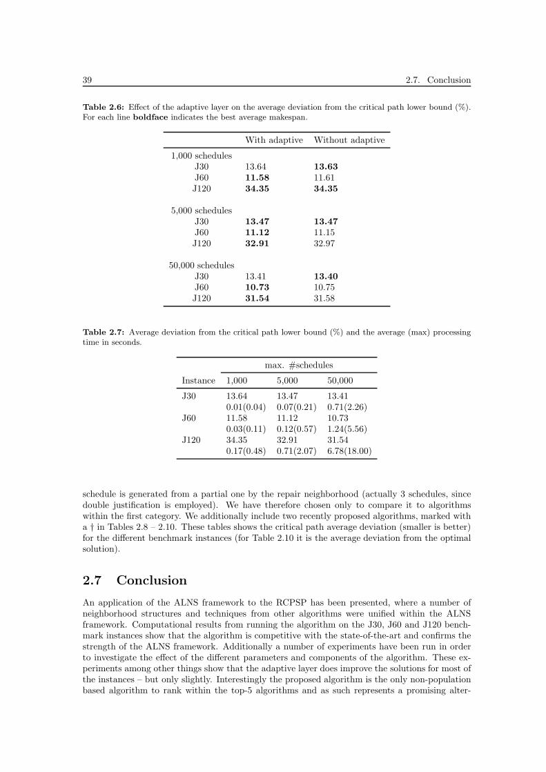
39 2.7. Conclusion
Table 2.6: Effect of the adaptive layer on the average deviation from the critical path lower bound (%).For each line boldface indicates the best average makespan.
With adaptive Without adaptive
1,000 schedulesJ30 13.64 13.63J60 11.58 11.61J120 34.35 34.35
5,000 schedulesJ30 13.47 13.47J60 11.12 11.15J120 32.91 32.97
50,000 schedulesJ30 13.41 13.40J60 10.73 10.75J120 31.54 31.58
Table 2.7: Average deviation from the critical path lower bound (%) and the average (max) processingtime in seconds.
max. #schedules
Instance 1,000 5,000 50,000
J30 13.64 13.47 13.410.01(0.04) 0.07(0.21) 0.71(2.26)
J60 11.58 11.12 10.730.03(0.11) 0.12(0.57) 1.24(5.56)
J120 34.35 32.91 31.540.17(0.48) 0.71(2.07) 6.78(18.00)
schedule is generated from a partial one by the repair neighborhood (actually 3 schedules, sincedouble justification is employed). We have therefore chosen only to compare it to algorithmswithin the first category. We additionally include two recently proposed algorithms, marked witha † in Tables 2.8 – 2.10. These tables shows the critical path average deviation (smaller is better)for the different benchmark instances (for Table 2.10 it is the average deviation from the optimalsolution).
2.7 Conclusion
An application of the ALNS framework to the RCPSP has been presented, where a number ofneighborhood structures and techniques from other algorithms were unified within the ALNSframework. Computational results from running the algorithm on the J30, J60 and J120 bench-mark instances show that the algorithm is competitive with the state-of-the-art and confirms thestrength of the ALNS framework. Additionally a number of experiments have been run in orderto investigate the effect of the different parameters and components of the algorithm. These ex-periments among other things show that the adaptive layer does improve the solutions for most ofthe instances – but only slightly. Interestingly the proposed algorithm is the only non-populationbased algorithm to rank within the top-5 algorithms and as such represents a promising alter-

Bibliography 40
Table 2.8: Average deviation from critical path lower bound (%) - J120
max. #schedules
Reference Algorithm 1,000 5,000 50,000
Valls et al. (2008) GA 34.07 32.54 31.24Ranjbar et al. (2009)† SS 35.08 33.24 31.49ALNS ALNS 34.35 32.91 31.54Debels et al. (2006)† SS 35.22 33.10 31.57Valls et al. (2005) GA 35.39 33.24 31.58Kochetov and Stolyar (2003) GA, TS 34.74 33.36 32.06Valls et al. (2005) GA 35.18 34.02 32.81Hartmann (2002) GA 37.19 35.39 33.21
Table 2.9: Average deviation from critical path lower bound (%) - J60
max. #schedules
Reference Algorithm 1,000 5,000 50,000
Ranjbar et al. (2009)† SS 11.59 11.07 10.64Debels et al. (2006)† SS 11.73 11.10 10.71Valls et al. (2008) GA 11.56 11.10 10.73ALNS ALNS 11.58 11.12 10.73Kochetov and Stolyar (2003) GA, TS 11.71 11.17 10.74Valls et al. (2004) GA 12.21 11.27 10.74Hartmann (2002) GA 12.21 11.70 11.21Hartmann (1998) GA 12.68 11.89 11.23
Table 2.10: Average deviation from optimal makespan (%) - J30
max. #schedules
Reference Algorithm 1,000 5,000 50,000
Ranjbar et al. (2009)† SS 0.10 0.03 0.00Kochetov and Stolyar (2003) GA, TS 0.10 0.04 0.00Debels et al. (2006)† SS 0.10 0.04 0.00Valls et al. (2008) GA 0.27 0.06 0.02ALNS ALNS 0.18 0.07 0.02Alcaraz and Maroto (2001) GA 0.33 0.12 -Valls et al. (2004) GA 0.34 0.20 0.02Tormas and Lova (2003a) sampling 0.25 0.13 0.05
native approach to the usual population based algorithms. Another encouraging sign is that thealgorithm ranks better on the larger and more difficult instances.
Bibliography
Alcaraz, J., Maroto, C. A robust genetic algorithm for resource allocation in project scheduling.Annals of Operations Research, 102:83–109, 2001.

41 Bibliography
Blazewicz, J., Lenstra, J., Kan, A. R. Scheduling subject to resource constraints: Classificationand complexity. Discrete Applied Mathematics, 5:11–24, 1983.
Bouleimen, K., Lecocq, H. A new efficient simulated annealing algorithm for the resource-constrained project scheduling problem and its multiple mode version. European Journal ofOperational Research, 149(2):268–281, 2003.
Brucker, P., Drexl, A., Mohring, R., Neumann, K., Pesch, E. Resource-constrained project schedul-ing: Notation, classification, models, and methods. European Journal of Operational Research,112(1):3–41, 1999.
Debels, D., Leus, R., Vanhoucke, M. A hybrid scatter search/electromagnetism meta-heuristic forproject scheduling. European Journal of Operational Research, 169(2):638–653, 2006.
Debels, D., Reyck, B. D., Leus, R., Vanhoucke, M. A decomposition-based genetic algorithm forthe resource-constrained project-scheduling problem. Operations Research, 55(4):457–469, 2007.
Fleszar, K., Hindi, K. S. Solving the resource-constrained project scheduling problem by a variableneighbourhood search. European Journal of Operational Research, 155(2):402–413, 2004.
Hartmann, S. A competitive genetic algorithm for resource-constrained project scheduling. NavalResearch Logistics, 45:733–750, 1998.
Hartmann, S. A self-adapting genetic algorithm for project scheduling under resource constraints.Naval Research Logistics, 49:433–448, 2002.
Herroelen, W., Demeulemeester, E., Reyck, B. D. Resource-constrained project scheduling - asurvey of recent developments. Computers & Operations Research, 29(4):279–302, 1998.
Kochetov, Y., Stolyar, A. Evolutionary local search with variable neighborhood for the resourceconstrained project scheduling problem. In Proceedings of the 3rd International Workshop ofComputer Science and Information Technologies, 2003.
Kolisch, R., Hartmann, S. Heuristic algorithms for solving the resource-constrained projectscheduling problem: Classication and computational analysis. In Weglarz, J., editor, Projectscheduling: Recent models, algorithms and applications, pages 147–178. Kluwer Academic Pub-lishers, Kluwer, Amsterdam, the Netherlands, 1999.
Kolisch, R., Hartmann, S. Experimental investigation of heuristics for resource-constrained projectscheduling. European Journal of Operational Research, 127:394–407, 2000.
Kolisch, R., Hartmann, S. Experimental investigation of heuristics for resource-constrained projectscheduling: An update. European Journal of Operational Research, 174(1):23–37, 2006.
Kolisch, R., Padman, R. An integrated survey of deterministic project scheduling. Omega, 29(3):249–272, 2001.
Kolisch, R., Sprecher, A. Psplib – a project scheduling library. European Journal of OperationalResearch, 96:205–216, 1996.
Nonobe, K., Ibaraki, T. Formulation and tabu search algorithm for the resource constrainedproject scheduling problem. In Ribeiro, C. C., P. Hansen, e., editors, Essays and Surveys inMetaheuristics, pages 557–588. Kluwer Academic Publishers, 2002.
Palpant, M., Artigues, C., Michelon, P. Lssper: Solving the resource-constrained project schedul-ing problem with large neighbourhood search. Annals of Operations Research, 131(1-4):237–257,2004.
Patterson, J. A comparison of exact approaches for solving the multiple constrained resource,project scheduling problem. Management science, 30(7):854–867, 1984.

Bibliography 42
Pisinger, D., Røpke, S. A general heuristic for vehicle routing problems. Computers & OperationsResearch, 34(8):2403–2435, 2007.
Pritsker, A. A. B., Watters, L. J., Wolfe, P. M. Multiproject scheduling with limited resources: Azero-one programming approach. Management Science, 16:93–108, 1969.
Ranjbar, M., Reyck, B. D., Kianfar, F. A hybrid scatter search for the discrete time/resourcetrade-off problem in project scheduling. European Journal of Operational Research, 193(1):35–48, 2009.
Røpke, S., Pisinger, D. A unified heuristic for a large class of vehicle routing problems withbackhauls. European Journal of Operational Research, 171(3):750–775, 2006a.
Røpke, S., Pisinger, D. An adaptive large neighborhood search heuristic for the pickup and deliveryproblem with time windows. Transportation Science, 40(4):455–472, 2006b.
Sprecher, A., Kolisch, R., Drexl, A. Semi-active, active and non-delay schedules for the resource-constrained project scheduling problem. European Journal of Operational Research, 80:94–102,1995.
Tormas, P., Lova, A. Integrating heuristics for resource constrained project scheduling: Onestep forward. Technical report, Department of Statistics and Operations Research, UniversidadPolitcnica de Valencia, 2003a.
Tormas, P., Lova, A. An efficient multi-pass heuristic for project scheduling with constrainedresources. International Journal of Production Research, 41:1071–1086, 2003b.
Valls, V., Quintanilla, S., Ballestın, F. Resource-constrained project scheduling: A critical activityreordering heuristic. European Journal of Operational Research, 149(2):282–301, 2003.
Valls, V., Ballestın, F., Quintanilla, S. A population-based approach to the resource-constrainedproject scheduling problem. Annals of Operations Research, 131:304–324, 2004.
Valls, V., Ballestın, F., Quintanilla, S. Justification and rcpsp: A technique that pays. EuropeanJournal of Operational Research, 165:375–386, 2005.
Valls, V., Ballestın, F., Quintanilla, S. A hybrid genetic algorithm for the resource-constrainedproject scheduling problem. European Journal of Operational Research, 185(2):495–508, 2008.

Chapter 3
An Adaptive Large Neighborhood Search
Algorithm for the Multi-mode
Resource-Constrained Project Scheduling
Problem
Laurent Flindt Muller
Department of Management Engineering, Technical University of DenmarkProduktionstorvet, Building 426, DK-2800 Kgs. Lyngby, Denmark
Abstract We present an Adaptive Large Neighborhood Search algorithm for the Multi-mode Re-
source-Constrained Project Scheduling Problem (MRCPSP). We incorporate techniques for deriving ad-
ditional precedence relations and propose a new method, so-called mode-diminution, for removing modes
during execution. These techniques make use of bound arguments, and we propose and experiment with
three new bounds for the MRCPSP, in addition to bounds found in the literature. We propose a simple
technique, so-called opportunistic mode-flipping, which can be applied whenever a schedule is generated,
and which significantly improves the results of the algorithm. Computational experiments are performed
on a set of standard benchmark instances from the PSPLIB, and a comparison is made with other algo-
rithms found in the literature. The experiments show that the algorithm is competitive, lying among the
three best heuristics found in the literature. Some of the elements of the algorithm perform well, that is
the bound arguments, the mode-removal procedure, and in particular opportunistic mode-flipping, and
these elements may perhaps be used to improve the results of other algorithms for this problem.
Keywords: Project scheduling, Heuristic, Large neighborhood search, Resource-constrained,Multi-mode
3.1 Introduction
Many processes within production scheduling and project management consists of scheduling anumber of activities, each activity having a certain duration and requiring a certain amount oflimited resources. Resources could for instance be machines or labor. Precedence relations mayexist between activities, such that one activity can not start before others are completed. Typicallyone wishes schedule to the activities such that the total time taken to complete them is minimized.Such problems can be modeled as a Resource-Constrained Project Scheduling Problem (RCPSP),which is a generalization of the well-known Job-Shop-Scheduling problem. There exists a numberof variants of the RCPSP, see for instance Blazewicz et al. (1983), Brucker et al. (1999), or
43

Chapter 3. An Adaptive Large Neighborhood Search Algorithm for the Multi-modeResource-Constrained Project Scheduling Problem 44
Hartmann and Briskorn (2010). We consider the the Multi-mode Resource-Constrained ProjectScheduling Problem (MRCPSP), which is a popular variant. In the MRCPSP each activity can beperformed in a number of different so-called modes, each representing alternative ways of executingthe activity.
There exists a large body of work for the Single-mode Resource-Constrained Project SchedulingProblem (SRCPSP) and to a lesser extend for the MRCPSP. We refer to the surveys by Hart-mann and Drexl (1998), Herroelen et al. (1998), Kolisch and Hartmann (2000, 2006), Kolisch andPadman (2001), and Patterson (1984). Among the heuristic solution methods for the MRCPSPare the immune-system based algorithm of Van Peteghem and Vanhoucke (2009), the (hybrid)genetic algorithms of Alcaraz et al. (2003), Hartmann (2001), Lova et al. (2009), Mori and Tseng(1997), Okada et al. (2010), Ozdamar (1999), Tseng (2008) and Tseng and Chen (2009), the tabu-search based algorithm of Tchao and Martins (2008), the simulated annealing-based algorithmsof Bouleimen and Lecocq (2003) and Jozefowska et al. (2001), the ant-colony optimization basedalgorithm of Chiang et al. (2008), the particle swarm optimization algorithm of Jarboui et al.(2008) and Zhang et al. (2006), the differential evolution based algorithm of Damak et al. (2009),the hybrid scatter search based algorithm of Ranjbar et al. (2009), and the local-search basedalgorithms of Boctor (1996), Drexl and Gruenewald (1993) and Kolisch and Drexl (1997). Cur-rently the best performing algorithms are the immune-system based algorithm of Van Peteghemand Vanhoucke (2009) and the genetic algorithm of Lova et al. (2009).
In this paper we experiment with an Adaptive Large Neighborhood Search (ALNS) algorithm,which is a heuristic procedure. The motivation for using an ALNS based algorithm is twofold:(1) ALNS is a relatively new meta-heuristic approach, which has been applied with good resultswithin the context of vehicle routing problems, and it would be of interest to see how the approachperforms in a different context. (2) The ALNS framework is very flexible, making it possible toincorporate different neighborhood structures and letting the adaptive layer of the ALNS algorithmselect among the best performing during execution. The hope is that using this approach toincorpore neighborhoods from state-of-the-art algorithms for the RCPSP into a single algorithm,will be beneficial. A similar approach was examined by Muller (2009) for the single-mode RCPSPwith moderate success, and the algorithm described here is an extension of the algorithm of Muller(2009).
We incorporate techniques for deriving additional precedence relations and propose and ex-periment with a new method for removing modes during execution (so-called mode-diminution).These techniques make use of lower bound arguments, and we propose and experiment with threenew lower (named LBX1, LBX2, and LB2X) for the MRCPSP, in addition to lower bounds foundin the literature. A preprocessing step, which strengthens these lower bounds, is also proposed(so-called resource strengthening). We finally propose and experiment with a simple techniquewhich can be applied every time a new schedule is generated, and which significantly improves theresults (so-called opportunistic mode-flipping). The technique can be seen as an extension of thesingle-pass improvement method used by Hartmann (2001) for his genetic algorithm.
Computational experiments are performed on a set of standard benchmark instances from thePSPLIB, and a comparison is made with other algorithms from the literature. These experimentsshow that the proposed algorithm is competitive, lying among the three best heuristics found inthe literature. Mode-diminution and in particular opportunistic mode-flipping perform well, andthe new lower bounds improve upon existing ones examined. Some of these elements may perhapssuccessfully be used to improve upon solutions for other heuristics for this problem. To the bestof our knowledge, this is the first application of an ALNS algorithm to the MRCPSP.
The remaining of the document is organized as follows: in Section 3.2 a formal description ofthe RCPSP is given, in Section 3.3 the ALNS framework is described, in Section 3.4 a number oflower bounds used in the al gorithm are presented along with three new lower bound methods,in Section 3.5 components of the propsed algorithm is presented. An ALNS heuristic include anumber of neighborhoods and these are described in Section 3.6. In Section 3.7 the computationalexperiments are presented, and we conclude in Section 3.8.

45 3.2. Problem description
3.2 Problem description
The MRCPSP can be described as follows (see for instance Brucker et al. (1999)): A projectconsists of a set A = {1, . . . , n} of activities, which must be scheduled. Traditionally activity 1and n are so-called dummy activities, which represent the start and the end of the project. Eachactivity j can be performed in a number of different modes Mj = {1, . . . , |Mj |}, each representinga different way of performing the activity. There are two sets of resources, (1) renewable resourcesR = {1, . . . , |R|}, and (2) nonrenewable resources R = {1, . . . , |R|}. A renewable resource k ∈ R,has capacity Rk in each time period, while a nonrenewable resource k ∈ R has capacity Rk spreadacross all time periods. When an activity j is scheduled in mode m ∈ Mj , it has a processingtime of pjm (non-preemtible) and requires rjkm ≥ 0 units of renewable resource k ∈ R in each
time period, and rjkm ≥ 0 of nonrenewable resource k ∈ R spread across all time periods. Thereexists precedence relations between the activities, such that one activity j ∈ A can not be startedbefore all its predecessors, Pj , are completed. Symmetrically Sj denotes the set of successors. LetE = {(i, j) ∈ A × A : i ∈ Pj} be the set of all precedence relations. Let T be a set of time-stepsduring which the activities must be performed. The MRCPSP may be formulated as follows:
min σn
s.t. σj ≥ σi + pi,m(i) ∀(i, j) ∈ E (3.1)∑
j∈A(t)
rj,k,m(j) ≤ Rk ∀k ∈ R, ∀t ∈ T (3.2)
∑
j∈A
rj,k,m(j) ≤ Rk ∀k ∈ R (3.3)
σj ≥ 0 ∀j ∈ A, (3.4)
where σj is the starting time of activity j, m(j) is the mode chosen for activity j, and A(t) = {j ∈A|σj ≤ t ≤ σj + pj,m(j)}, i.e., the activities in progress at time t. Constraints (3.1) are denotedthe precedence constraints, constraints (3.2) are denoted the renewable resource constraints, andconstraints (3.3) are denoted the nonrenewable resource constraints. As mentioned previously theRCPSP (and thus also the MRCPSP) is a generalization of the Job Shop Scheduling Problem andis therefore NP-hard (see e.g. Blazewicz et al. (1983)).
3.3 Adaptive large neighborhood search
The ALNS framework was first proposed by Pisinger and Røpke (2007) for solving different variantsof vehicle routing problems, and promising results have been reported by Pisinger and Røpke(2007) and Røpke and Pisinger (2006a,b). It is a framework which can be applied to a large classof optimization problems and can be described as follows: ALNS is a local search framework inwhich a number of simple neighborhoods compete to modify the current solution. In each iterationa destroy neighborhood is chosen to destroy the current solution, and a repair neighborhood ischosen to repair the solution. The new solution is accepted if it satisfies some criteria defined bythe local search method applied at the master level. The neighborhoods used are typically largeneighborhoods, which can reach a large part of the solution space.
An adaptive layer stochastically controls which neighborhoods to choose based on their pastperformance (score). The more a neighborhood has contributed to the quality of the currentsolution, the larger score it obtains, and hence has a larger probability of being chosen. Theadaptive layer uses roulette wheel selection for choosing one of the destroy and one of the repairneighborhoods. If the past score of a neighborhood i is πi and we have ω neighborhoods, thenwe choose neighborhood j with probability πj/
∑ωi=1 πi. ALNS can be based on any local search
method, e.g., simulated annealing, tabu search or guided local search. An outline of the ALNSframework is given by Algorithm 3.1. For a more detailed description we refer to Pisinger andRøpke (2007).

Chapter 3. An Adaptive Large Neighborhood Search Algorithm for the Multi-modeResource-Constrained Project Scheduling Problem 46
Algorithm 3.1 Outline of the ALNS framework
1: Construct feasible solution x.2: x∗ ← x3: while stop criteria not met do4: Choose a destroy neighborhood N− and repair neighborhood N+ using roulette wheel se-
lection based on previously obtained scores {πj}.5: Generate a new solution x′ from x using the heuristics corresponding to the chosen destroy
and repair neighborhoods, N− and N+.6: if x′ can be accepted then7: x← x′
8: end if9: Update scores πj of N− and N+.
10: if f(x) < f(x∗) then11: x∗ ← x12: end if13: end while14: return x∗
3.4 Lower bounds
Good lower bounds are an important component in branch-and-bound algorithms in order to beable to prune the search tree effectively. They may also prove useful in a heuristic setting, wherethey may be used to speed up the heuristic by terminating early when an optimal solution has beenfound, or to restrict the heuristic to parts of the solution space, where improving solutions may befound. In order to find lower bounds, we make use of a so-called Finish-to-Start-Distance (FSD)-matrix and a number of lower bound arguments, and we in the following give a formal presentationof the FSD-matrix and the lower bounds employed.
Finish-to-Start-Distance (FSD)-matrix We employ a slight modification of the FSD-matrixof Zhu et al. (2006), which is in itself a modification of the traditional Start-to-Start distancematrix found in the literature, see for instance Bartusch et al. (1988), Brucker and Knust (2000),or Demassey et al. (2005). An FSD-matrix is an integer matrix, B = (bij)A×A, which satisfies:
σj − τi ≥ bij + 1, ∀(i, j) ∈ A×A
for all feasible schedules, where τi is the completion time of activity i and σj is the starting timeof activity j. That is bij is a lower bound on the amount of time which must pass between thecompletion time of i and the starting time of j. Note that bij may be negative, which means thatactivity j must start before the completion of activity i. Define p
i:= min{pim|m ∈ Mi} and
pi := max{pim|m ∈ Mi}. Since the relation (3.4) has the following transitive property:
σj − τi ≥ bij + 1 ∧ σk − τj ≥ bjk + 1⇒ σk − τi ≥ bij + pj+ bjk + 1,
the entries of an FSD-matrix may be updated by calculating the transitive closure of B. This canbe done using a variant of the Floyd-Warshall algorithm in O(|A|3) time, see Zhu et al. (2006).Note that a pair of activities (i, j) must run in parallel if bij ≥ −pi−p
j+1 and bji ≥ −pi−p
j+1.
Given an upper bound, T , on the makespan the FSD-matrix B may be initialized as follows:
bij =
−pi if i = j0 if (i, j) ∈ E−T otherwise,
The difference between the FSD-matrix considered here, and the one of Zhu et al. (2006) is thathere the FSD-matrix is defined for all pairs of activities, whereas it in Zhu et al. (2006) is definedonly for pairs of activities being related by precedence.

47 3.4. Lower bounds
As will be explained in detail in Section 3.5, an FSD-matrix may be used to discover new prece-dence relations, to eliminate modes from consideration, and to prove optimality. The effectivenessof the methods rely on good lower bound arguments for the bij values. The values bij may be cal-culated by constructing the subproblem induced by Si∩Pj and then applying any lower boundingtechnique for the RCPSP on this smaller instance. A number of such lower bounds exists in theliterature. We do not give a description of these here but instead refer the reader to the excellentwork by Klein and Scholl (1999) where 11 such lower bounds are described and compared. Usingthe name convention of Klein and Scholl (1999), the lower bounds considered here are: LB1, LB2,LB6, LB8, LB10, and LB11. LB1 is the well-known critical path lower bound, LB2 is the alsowell-known capacity bound (explained in more detail below), LB6 and LB8 are extensions of theso-called weighed node packing bound of by Mingozzi et al. (1998) (see Klein and Scholl (1999)),and LB10 and LB11 are lower bounds based on evaluating a lower bound for all possible ways ofresolving a resource conflict given respectively pairs, and triples of activities (again see Klein andScholl (1999)).
The lower bounds LB6, LB10, and LB11 themself use lower bound arguments on subproblemsof the problem for which the lower bound is calculated. Recall that this problem may in itselfbe a subproblem corresponding to a bij entry. In order to to distinguish the two, we will referto subproblems used within the calculation of the lower bounds LB6, LB10, and LB11 as innersubproblems. When calculating lower bounds on inner subproblems, one could recursively applylower bound arguments, but this can potentially by very time-consuming, and we thus, like Kleinand Scholl (1999), only apply the critical path lower bound (LB1) and capacity bound (LB2).For the computational experiments we will investigating replacing LB2 with an extended variant(LB2X described below), which provides better lower bounds, but at the cost of additional runningtime.
In the following we describe three new lower bounds (LBX1, LBX2, and LB2X) for theMRCPSP. These lower bounds are improvements of the critical path lower bound (LB1), andcapacity lower bound (LB2), and we begin with a short description of the latter.
LB1 (critical path) This lower bound is computed by finding the longest path (also called thecritical path) in the precedence graph. For the multi-mode case this critical path is calculatedbased on the minimum processing time of each activity.
LB2 (capacity bound) For a activity i ∈ A, define aikm := pimrikm/Rk and let aik =minm∈Mi
{aikm}. This lower bound is calculated as
LB2 = maxk∈R
{⌈
∑
i∈A
aik
⌉}
,
i.e., it is a lower bound based on the amount of renewable resource available versus the amountof renewable resource required by a set of activities.
LBX1 (mode-fixed critical path 1) Let I be some multi-mode instance. Let LB1(I) andLB2(I) denote the lower bounds as computed by the lower bounds LB1 and LB2 above. For asubset S ⊆ A let MS denote the set of feasible mode assignments for the activities of S. Fora feasible mode assignment m ∈ MS , let I(m) denote the corresponding restriction of I to theselected modes. It is clear that the lower bound calculated as
LB = maxS∈S
minm∈MS
max{LB1(I(m)), LB2(I(m))},
where S is some powerset of A, is a strengthening of LB1 and LB2 in the multi-mode case. As thenumber of feasible mode assignments grows exponentially in the size of S, S must be kept smallin order for the lower bound to be computationally tractable. LBX1 is calculated as above, whereS is the set of all pairs of activities from A.

Chapter 3. An Adaptive Large Neighborhood Search Algorithm for the Multi-modeResource-Constrained Project Scheduling Problem 48
LBX2 (mode-fixed critical path 2) LBX1 may be improved by considering larger subsets ofactivities. LBX2 is calculated as LBX1, except S is the set of all pairs, and triples of activities ofA.
LB2X (extended capacity bound) The capacity bound LB2 above is calculated separately foreach resource. In the multi-mode case the lower bound may be strengthened by taking into accountall the resources simultaneously. Finding the best lower bound using this approach amounts tosolving the following Mixed Integer Programming (MIP) problem:
min b (3.5)
s.t.∑
i∈A
∑
m∈Mi
aikmxim ≤ b ∀k ∈ R (3.6)
∑
m∈Mi
xim ≥ 1 ∀i ∈ A (3.7)
b ≥ 0 (3.8)
xim ∈ {0, 1} ∀i ∈ A,m ∈Mi (3.9)
where xim = 1 if and only if activity i uses mode m.
Proposition 3.1. The MIP problem (3.6) – (3.9) is NP-hard.Proof. We show this by reduction from the NP-hard partition problem (see Karp (1972)), whichin its optimization version asks: Given a set C of integer numbers, find a partition of C into twosubsets C1 and C2 such that max(sum(C1), sum(C2)) is minimized. The reduction is as follows:Let |R| = 2 and let each resource have unit capacity. For each c ∈ C, create an activity i withtwo modes with resource usages (c, 0) and (0, c).
As the problem (3.6) – (3.9) is NP-hard we instead consider a Lagrangian relaxation, wherethe constraints (3.6) have been dualized. This gives rise to the following Langragian Dual (LD)problem:
maxλk≥0
,∑
k∈R λk≤1
min∑
k∈R
λk
∑
i∈A
∑
m∈Mi
aikmxim (3.10)
s.t.∑
m∈Mi
xim ≥ 1 ∀i ∈ A (3.11)
xim ∈ {0, 1} ∀i ∈ A,m ∈Mi, (3.12)
For any choice of λ the problem may be solved in linear time. Note that if one chooses λk = 1and λk′ = 0 ∀k′ 6= k, then the solution to the inner minimization problem is the same as LB2calculated on the resource k. The LD problem can be solved by using a subgradiant algorithm.
LB2X is defined as the best solution found after a specified number of iterations of the sub-gradiant algorithm. The number of iterations has been experimentally fixed to 40.
As we will see later applying subgradiant algorithm may prove too slow in certain cases, whenthe lower bound is used for the inner subproblems. We thus define an additional lower bound,LB2X’, which is faster to compute, but also weaker: the lower bound is defined as the best solutionto the LD problem for a fixed number of of values of λ (|R|+1 values in total). These values of λare λk = 1 and λk′ = 0 ∀k′ 6= k, where k = 1 . . . |R| (giving |R| values of λ), and λk = 1/|R| ∀k ∈ R(giving one additional value of λ).
3.5 Algorithm
The algorithm proposed is an extension to the MRCPSP of the algorithm presented in Muller(2009) for the single-mode RCPSP. For the sake of completion we here repeat the elements fromthat algorithm, which are relevant for the extension, and describe some new elements specific tothe extension.

49 3.5. Algorithm
Representation A number of different solution representations of the RCPSP has been pro-posed in the literature (see for instance Kolisch and Hartmann (1999)). The proposed algorithmemploys list representation, where a schedule is represented as an ordered list of activities. Theordering is as follows: Let (i, j) ∈ E and let γi and γj be the positions within the list of activity iand j respectively, then γi < γj .
When employing list representation, one additionally needs a scheme for converting the list intoa schedule. The two most commonly used are the serial and parallel Schedule Generation Schemes(SGSs) (see for instance Kolisch and Hartmann (1999)). For the ALNS algorithm examined inMuller (2009), in context of the SRCPSP the serial SGS turned out to produce better solutionsthan the parallel SGS and we therefore used the serial SGS here. The serial SGS can be describedas follows: in the order defined by the list, schedule each activity in turn, at the earliest precedenceand resource feasible point in time.
Local search method As noted in Section 3.3 one needs to select a local search method ontop of which to build the ALNS algorithm. The method used here is as follows: In each iterationa destroy and repair neighborhood is selected based on the current scores. Given the parameterQ, which governs how many activities may be moved within the current list, a new schedule (andcorresponding activity list) is created based on the neighborhoods selected. Only solutions whichare as good as, or better than, the current solution are accepted. A tabu list is maintained toensure that the same activity list is not visited twice. The value Q is progressively reduced fromits initial value toward a final low value. This has the effect that in the beginning the algorithmwill look at large neighborhoods, but as the search progresses to good solutions the size getsprogressively reduced. The idea is that when a good solution has been found, the overall structureof the solution is sound and should be kept but small changes may find a new better solution.
Scoring scheme As part of an ALNS algorithm, a scoring scheme for the destroy and repairneighborhoods needs to be decided upon. As in Pisinger and Røpke (2007) we update the scoresat regular intervals rather than in each iteration. Thus scoring information is collected during anumber of iterations before the scores of each neighborhood is updated and the collection restarts.In the following we use the same naming convention as Pisinger and Røpke (2007). Let the scoreinterval be the number of iterations which must pass between each score update. Let πj be thecurrent score, i.e., the score on the basis of which neighborhoods are chosen, and let πj the scoreaccumulated during the score interval (it will be explained later how πj is accumulated). Thescore πj is updated as follows at the end of a score interval: πj = max{ρ · πj
aj+ (1− ρ) · πj , πmin},
where aj is the number of times the neighborhood has been chosen during the last score interval(if aj = 0, the score remains identical to the score in the previous interval), ρ is the score reactionand πmin is a minimum score.
Let |Sx| be the makespan of the current solution, |Sx∗ | the makespan of the current bestsolution, and |Sx′ | the makespan of the current candidate created by applying the destroy andrepair neighborhood N+ and N−. Let πj be the collected score so far for N+ (the procedure isequivalent for N−), πj is updated as follows:
πj = πj +
10 if |Sx′ | < |Sx∗ |5 if |Sx′ | < |Sx|2|Sx|−|Sx′ |−1 otherwise
This scoring scheme differs slightly from the one employed in Pisinger and Røpke (2007), whereone of three fixed scores are attributed depending on whether the current solution was improvedglobally, locally or a worse solution was accepted. The reason for this difference is that theproposed algorithm only accepts equal or better solutions (while the local search method employedin Pisinger and Røpke (2007) may accept worse solutions), which can results in many iterationswhere there is no improvement at all. If a fixed scoring scheme was used all neighborhoodswould be scored equally bad, while for the employed scheme it is possible to differentiate theneighborhoods who produce solutions which are (almost) as good as the current and the ones that

Chapter 3. An Adaptive Large Neighborhood Search Algorithm for the Multi-modeResource-Constrained Project Scheduling Problem 50
produce solutions which are far worse. Note that even though only better solutions are accepted,the middle case above may occur because the mode-change-algorithm, precedence augmentation,and mode diminution procedures (see later) may result in the current solution being worse thanthe best found solution.
Modes Throughout the course of the algorithm a feasible mode-selection is maintained. Notethat finding a feasible mode selection is in itself an NP-hard problem. In the initial stage ofthe algorithm a feasible mode-selection is found by applying the Minimum Normalized Resources(MNR) method of Lova et al. (2009). For the few cases, where this method can not find an feasiblemode-selection, we apply exhaustive search.
The destroy and repair neighborhoods work only on the current mode-selection. At regularintervals a mode-change-algorithm is run, which attempts to find a new mode selection, whichthen become the current until the next call to the mode-change-algorithm.
Let UB be the current upper bound, then the new mode-selection should be such that the lowerbound does not exceed UB − 1, otherwise no improving solution can be found using that mode-selection. In order not to spend too much time searching for mode-selections with LB ≤ UB−1 (iffor instance, the optimal solution has already been found, such a mode-selection may not exists),the frequency of calls to the mode-change-algorithm is halved when no new mode-selection couldbe found. Initially this frequency is set to 2, i.e., every other iteration of the ALNS algorithm.The mode-change-algorithm can be seen in Algorithm 3.2.
Algorithm 3.2 Pseudocode for the mode-change-algorithm
for all distinct triples (i, j, k) ∈ A×A×A dofor all mode combinations (mi,mj ,mk) ∈Mi ×Mj ×Mk doif change to (mi,mj ,mk) is feasible thenMake change, and calculate lower bound: LB.if LB ≤ UB − 1 thenDouble call-frequency (if previously halved).return new mode-selection
end ifProceed with a new triple.
end ifend for
end forHalve call-frequency.return new mode-selection (does not satisfy LB ≤ UB − 1)
Initial mode and resource reductions As described by Sprecher et al. (1997) the numberof modes and resources may be reduced by application of the following preprocessing procedure:Define rik := min{rikm|m ∈ Mi}, and rik := max{rikm|m ∈ Mi}. A mode m ∈ Mi is callednon-executable if either (1) rikm > Rk, for some k ∈ R, or (2)
∑
j∈A\{i} rjk + rikm > Rk, for
some k ∈ R. A mode is called inefficient if there exits another mode m′ of Mi, such thatrikm ≥ rikm′ ∀k ∈ R, and rikm ≥ rikm′ ∀k ∈ R. A nonrenewable resource k is called redundantif∑
i∈A rik ≤ Rk. Non-executable and inefficient modes, and redundant nonrenewable resourcescan be removed initially by the use of the algorithm described in Algorithm 3.3. This procedure isalso used by Alcaraz et al. (2003), Hartmann (2001), Jozefowska et al. (2001), Okada et al. (2010),Ranjbar et al. (2009), and Tseng and Chen (2009) for their algorithms.
Initial resource strengthening The lower bounds LB2, LB2X, and LB2X’ are dependantupon the resource usages. If the resource usage of an activity in a certain mode can be increasedwithout changing the optimal solution, the resulting bounds will be stronger. The following rule

51 3.5. Algorithm
Algorithm 3.3 Pseudocode for preprocessing of modes and nonrenewable resources
Remove non-executable modes.repeatRemove redundant nonrenewable resources.Remove inefficient modes.
until No mode removed
is thus applied after the initial mode and resource reductions: Let (i, j) ∈ A × A be a pair ofactivities. We say that two modes mi ∈Mi and mj ∈ Mj are incompatible if they can not be runin parallel, either because of precedence relations between the activities, or because of resourceconstraints. If a mode m ∈Mi of an activity i ∈ A, is found, which is incompatible with all othermodes of all other activities, then the resource usage is updated as rikm := Rk ∀k ∈ R.
Precedence augmentation When a new upper bound, UB, is found, one is only interestedin finding better solutions. Thus any sequencing of activities which has a lower bound largerthan UB − 1 can be forbidden. Let the head, hj , of an activity j ∈ A be the time that mustpass before activity j can be started and let the tail, tj , be the time that must pass from thepoint where activity j has completed until the project can be completed. The head and tail ofan activity j can respectively be read from the entries b0j and bjn of the FSD-matrix. Definerik := min{rikm|m ∈ Mi}. We now describe how precedence relations may be deduced on thebasis of heads and tails.
The following two rules (3.13) and (3.14), are a simple generalization to the multi-mode caseof rules employed by Fleszar and Hindi (2004) in their variable neighborhood search algorithm.Let i, j ∈ A be a pair of activities for which no precedence relations exists. Precedence relationsmay be deduced as follows:
hj + ti ≥ UB ⇒ i→ j (3.13)
∃k ∈ R : rik + rjk > Rk ∧ hj + pj+ p
i+ ti ≥ UB ⇒ i→ j. (3.14)
We additionally use the following deduction rule: Let i, j, k ∈ A be a triple of activities forwhich no precedence relation exists and assume that none of the three can be run in parallel. Weexamine all 6 sequencing possibilities of the three activities: (1) i → j → k, (2) i → k → j, (3)j → i → k, (4) j → k → i, (5) k → i→ j, and (6) k → j → i. Given a sequencing, a → b→ c, alower bound on the makespan is ha + p
a+ p
b+ p
c+ tc. In the following let LB(1), . . . , LB(6) be
lower bounds corresponding to the sequences (1)–(6). New precedence relations may be deducedas follows:
LB(1) ≥ UB ∧ LB(2) ≥ UB ∧ LB(5) ≥ UB ⇒ j → i
LB(3) ≥ UB ∧ LB(4) ≥ UB ∧ LB(6) ≥ UB ⇒ i→ j
LB(1) ≥ UB ∧ LB(2) ≥ UB ∧ LB(3) ≥ UB ⇒ k → i
LB(4) ≥ UB ∧ LB(5) ≥ UB ∧ LB(6) ≥ UB ⇒ i→ k
LB(1) ≥ UB ∧ LB(3) ≥ UB ∧ LB(4) ≥ UB ⇒ k → j
LB(2) ≥ UB ∧ LB(5) ≥ UB ∧ LB(6) ≥ UB ⇒ j → k
When new precedence constraints are added, the current solution may become infeasible andneeds to be “repaired” for the search to go on. Sometimes, this results in the new solution havinga worse makespan than the solution on the basis of which precedence relations were added, whichis inconvenient since the search will continue from this worse solution. It is thus worthwhile tospend some time repairing a solution such that it is at least as good as the original one. To thisend, Fleszar and Hindi (2004) construct a special repair algorithm. We take a different approachand use the repair neighborhoods: a partial activity list, and a corresponding set of activities tobe reinserted is constructed as follows: Scan through the activity list of the current solution, if

Chapter 3. An Adaptive Large Neighborhood Search Algorithm for the Multi-modeResource-Constrained Project Scheduling Problem 52
an activity is encountered for which a least one predecessor has not yet been encountered, removethat activity from the list. Each repair neighborhood is in turn given a chance to repair thesolution until either a solution which is at least as good as the original is found or there are noneighborhoods left, in which case the repaired solution with the best makespan is used.
Mode diminution As is the case with precedence augmentation, when a new upper bound,UB, is found, only subsequent improvements is of interest. Thus modes, which lead to a lowerbound larger than UB − 1 may be removed. When a new UB is found a mode m ∈ Mi of anactivity i ∈ A is removed, if one of the following expressions are true:
1. hi + pim + ti ≥ UB.
2. bii ≥ −pim + 1 .
3. The current entries of the FSD-matrix implies i must run in parallel with some activity j,and m is incompatible with all modes of j.
If condition 2 is satisfied the mode can be removed because the condition implies σi + pim −1 > τi. The removal of a mode may render other modes non-executable, and may render somenonrenewable resources redundant. Thus the two first steps of Algorithm 3.3 are repeated, if amode is removed.
As for precedence augmentation, the removal of modes may render the current solution in-feasible. If this is the case new modes must be selected for the affected activities. We employa two-step approach: Let i ∈ A be some affected activity. First try to select from among theremaining modes of i one that satisfies the nonrenewable resource constraints. If no such modeexists, then construct a new mode-selection as for the initial schedule. If this fails, stop.
Early termination Throughout the course of the algorithm a lower bound is maintainedthrough the entries of the FSD-matrix. If at any point the current upper bound equals thelower bound, the search may be halted, as an optimal solutions has been found. One way tocalculate lower bounds is through so-called destructive arguments (see Klein and Scholl (1999)):Assume a minimization problem, with integer-valued objective function f(x), has to be solved, andthat a lower bound LB is known. A so-called restricted problem is formed, where the constraintf(x) ≤ LB is added. This constraint is then, via the application of so-called reduction algorithms,used to discover new constraints or modify the problem data so as to strengthen the formulation.If the problem is discovered to be infeasible, then the lower bound may be improved to LB + 1.
The process of imposing an upper bound of T = UB−1, when a new solutions has been found,updating the entries of the FSD-matrix, and subsequently applying precedence augmentation andmode diminution, can be seen as the application of such reduction algorithms. If through thisprocess the problem is found to be infeasible, the current UB is optimal. The following infeasibilitychecks are performed:
1. Some i ∈ A exists such that bii ≥ −pi + 1.
2. Some pair (i, j) exists such that i and j must run in parallel, and this is not feasible for anycombination of modes.
3. Some triple (i, j, k) exists such i, j and k must be run in parallel, and this is not feasible forany combination of modes.
One could also perform additional infeasibility checks, such as considering even larger sets of activ-ities, but there is a trade-off between the gain of early termination and the time spent performingthese tests.

53 3.5. Algorithm
Justification Valls et al. (2004) shows that a simple technique denoted justification can be eas-ily added to algorithms for the RCPSP, improving the quality of the solution with little extracomputational effort. One speaks of left-justification, right-justification and double-justification.Left-justification is essentially pulling all activities of a schedule as far towards time zero (left) aspossible, while right-justification is essentially pulling all activities as far towards the time corre-sponding to the makespan (right) as possible. Double-justification consists of a right-justificationfollowed by a left-justification. Sometmies a double-justified schedule is better than the originalone. Since this is a simple technique, which has been shown to produce good results, all schedulesproduced during the course of the ALNS algorithm are double-justified. This means that in eachiteration at least three schedules are generated (more may be generated if the current solutionmust be repaired after precedence augmentation). The number of schedules generated in eachiteration is important since the total number of generated schedules is used as a stopping criteriawhen comparing to other heuristics from the literature.
Opportunistic mode-flipping As for justification, opportunistic mode-flipping is a simple tech-nique, which is applied after the generation of a new schedule, and which may result in an im-provement. Let i ∈ A be some activity, and let m ∈Mi be the mode in which i is scheduled. Letm′ 6= m be some other mode of i. If changing the mode of i from m to m′ does not result in anincrease of the makespan, we denote the change a makespan-preserving mode-flip.
Proposition 3.2. Let m(i) be the current mode of an activity i ∈ A for the schedule S. Letσi be the starting time of i, let ξi = min{σj | j ∈ Si}, be the earliest starting time of a successorof i, and let R(t0, t1)ik = min{Rk −
∑
j∈A(t)\{i} rjkm(j)| t ∈ [t0, t1]}, be the minimum amount of
capacity left in the interval [t0, t1] on the resource k ∈ R. Let m′ 6= m(i) be some other mode ofi. If R(σi, σi + pim′)ik ≥ rikm′ ∀k ∈ R ∧ σi + pim′ ≤ ξi, then changing m to m′ is a makespan-preserving mode-flip.
Proof. R(σi, σi+ pim′)ik ≥ rikm′ ∀k ∈ R ensures that no activity scheduled in parallel with i afterthe flip, has to be moved earlier or later. The only other effected activities could be successors ofi, but σi + pim′ ≤ ξi ensures these do not have to be moved either.
Opportunistic mode-flipping is applied every time a new schedule is generated: In the orderdefined by the activity list each activity is examined to see if a makespan-preserving mode-flipmay be performed. If so, it is done. If more than one makespan-preserving mode-flip exists forthe same activity, the one resulting in the shortest processing time is performed.
The procedure can be seen as an extension of the single-pass improvement method used byHartmann (2001). The single-pass improvement method is itself based on the definition of the so-called multi-mode left shift bounding rule originally used in an exact algorithm, see Sprecher et al.(1997). The difference between the procedure of Hartmann (2001) and the procedure proposedhere is that for the former only mode-flips, which results in shorter processing times are performed,while this is not the case for the latter.
Overview An overview of the algorithm can be seen in Algorithm 3.4, where x indicates an ac-tivity list, while Sx is the associated schedule after it has been generated and |Sx| is the makespan.Lines 1–2 corresponds to the initial mode and resource reductions, and the initial resource strength-ening. Lines 5–11 corresponds to the propagation of lower bounds, and subsequent application ofprecedence augmentation and mode diminuation. Lines 13–15 is where the mode-change algorithmis called. On Line 16 the destroy and repair neighborhoods are chosen, and a new activity list iscreated. Finally on Line 18 a new schedule is generated and double justification and opportunisticmode-flipping is applied.

Chapter 3. An Adaptive Large Neighborhood Search Algorithm for the Multi-modeResource-Constrained Project Scheduling Problem 54
Algorithm 3.4 Pseudocode for the ALNS algorithm
Require: Initial values of Q and c, the initial scores {πj} and the #schedules max.1: Remove non-executable and inefficient modes and redundant nonrenewable resources.2: Strengthen resource constraints.3: s← 0, LB ← lower bound.4: Create an initial solution Sx∗ .5: Do precedence augmentation and mode diminution using |Sx∗ | as upper bound. If this results
in a better lower bound store it in LB.6: if x∗ is no longer precedence feasible then7: Repair x∗ using the repair neighborhoods and store the best found schedule in Sx. If this
results in a better makespan then store it as Sx∗ .8: end if9: if x∗ is no longer mode feasible then
10: Find new mode-selection for x∗. If this results in a better makespan then store it as Sx∗ .11: end if12: while s < max and |Sx∗ | > LB do13: if iterations since last run of mode-change-algorithm is large enough then14: Run mode-change-algorithm15: end if16: Choose a destroy and repair neighborhood (N−, N+) based on {πj} and create a new
candidate activity list x′ from the current schedule Sx.17: if not Tabu(x′) then18: Create a new candidate schedule Sx′′ from x′ using serial SGS, double justification, and
opportunistic mode-flipping.19: if |Sx′′ | < |Sx∗ | then20: Sx∗ ← Sx′′
21: Repeat the procedure from line 5 – 11 with the new best solution Sx∗ .22: else if |Sx′′ | ≤ |Sx| then23: Sx ← Sx′′
24: end if25: end if26: Q← c ·Q27: Update the number of generated schedules s.28: Update the scores πj for N− and N+
29: end while30: return Sx∗
3.6 Neighborhoods
An important part of an ALNS algorithm are the destroy and repair neighborhoods. Even thoughthere is an adaptive layer, one should remain careful about adding too many neighborhoods,especially when only a limited number of iterations is allowed. The reason is that a number ofiterations will be needed before any neighborhoods performing poorly on the current instance willhave been filtered out, and these neighborhoods will end up taking time from the good ones. It isalso important to have a good mix of neighborhoods, which are good at search intensification anddiversification. In the following we describe the destroy and repair neighborhoods employed.
Destroy neighborhoods Given the parameterQ and an activity list, L, a destroy neighborhoodmust remove Q activities from L. Some of the destroy neighborhoods share the same structure:A predicate function marks activities from L. The marked activities are then removed at randomfrom L along with zero or more activities relating to the ones removed, until Q activities areremoved, or no more marked activities are left. More formally: For j ∈ A the predecessor-

55 3.6. Neighborhoods
cluster of j is defined as Cp(j) = {i ∈ A|i ∈ Pj ∨ σi + pim(i) = σj}, and the cluster of j asCc(j) = {i ∈ A|i ∈ Cp(j) ∨ i ∈ Sj ∨ σj + pjm(i) = σi}, where σj denotes the starting timeof activity j. Let p : A → {0, 1} be some predicate, then a core removal candidate set, C, isconstructed as C = {j ∈ A|p(j) = 1}. At random an activity j from C is removed from the listalong with elements from either Cp(j) or Cc(j) (depending on the neighborhood) until either theset C is empty or Q elements have been removed from L.
The idea behind clusters is that one wants as much flexibility as possible for the repair neighbor-hood, e.g., if all the predecessors and successors of an activity are left in place there is potentiallylittle room for inserting the activity in new positions.
There are in total 10 destroy neighborhoods, which are described below.
• random (two flavors) This neighborhood ensures diversification by randomly removing Qactivities from the current solution. It comes in two flavors, one where predecessor-clusteringis used and one where clustering is used.
• most-mobile Let j ∈ A. As in Fleszar and Hindi (2004), we define the left limit LL(j) andthe right limit RL(j) as LL(j) = max{γi|i ∈ Pj}+1 and RL(j) = min{γi|i ∈ Sj}−1, whereγi is the position of i within the activity list. Now, the mobility, mob(j), of j is defined asmob(j) = RL(j)− LL(j).
This neighborhood selects the Q activities with the highest mobility from the current activitylist and also ensures diversification, but in a different way than the random neighborhooddescribed above. It ensures that the neighborhood explored is large by selecting activitieswhich have many reinsertion possibilities.
• non-peak (two flavors) In the hybrid genetic algorithm proposed by Valls et al. (2008) thepeak crossover operator employed passes on to its children the parts of the schedules withhigh utilization, so-called peaks. Similarly we define a non-peak predicate. A peak is definedin the same way as by Valls et al. (2008): Given a schedule, S, the Resource UtilizationRatio is defined as follows
RUR(t) =1
|R| ·∑
j∈A(t)
∑
k∈R
rjkRk
Given some δ ∈ [0; 1] we say that a point in time, t, is of high utilization if RUR(t) ≥ δ.Similarly we say that a time interval I is of high utilization if ∀t ∈ I : RUR(t) ≥ δ. LetI be the set of disjunctive maximal intervals of high utilization for the schedule S, then apeak activity j ∈ A is an activity which satisfies ∃I ∈ I : [σj ;σj + pjm(j)] ∩ I 6= ∅, i.e., allactivities, which are active during some interval of high utilization. A non-peak activity isan activity which is not a peak activity. The non-peak predicate selects all activities, whichare non-peak activities.
This neighborhood uses the non-peak predicate and tries to preserve the structure of thesolution where the utilization is good, and destroy the parts where it is not. The neighbor-hood comes in two flavors one where predecessor-clustering is used and one where clusteringis used. In both cases the activities are chosen at random from the removal candidate set.
• critical-path (two flavors) Given the current schedule S we construct a weighted directedgraph G = (A, E), where E = {(i, j) ∈ A × A|σi + pim(i) = σj} and the weight of avertex j is pjm(j). Since the schedule S does not contains “holes” where no activities arein progress, there must exist at least one path with weight equal to the makespan of S. Inorder to improve the makespan, at least one of the activities on this path must be movedelsewhere. The critical-path predicate selects all activities, which are part of a critical pathand at random selects Q for removal. The neighborhood comes in two flavors, one wherepredecessor-clustering is used and one where clustering is used.
• segment This neighborhood ensures a certain intensification by selecting a subsequence oflength Q from the activity list. This subsequence corresponds to a sub-schedule, which canhopefully be improved.

Chapter 3. An Adaptive Large Neighborhood Search Algorithm for the Multi-modeResource-Constrained Project Scheduling Problem 56
• time-windows (two flavors) Let the head and tail of an activity j be given by hj andtj respectively, and let UB be the current upper bound. For any schedule to improve uponthis upper bound, j must be scheduled in the interval [hj ;UB − tj − (pjm(j) − p
j)]. The
time-window predicate selects all activities which are scheduled outside this interval in thecurrent schedule.
The neighborhood comes in two flavors, one where predecessor-clustering is used and onewhere clustering is used. The activities from the candidate set are chosen at random. If thecandidate set has less than Q elements, additional activities are randomly chosen.
Repair neighborhoods Given a partial activity list and a set of activities to be reinserted arepair neighborhood must construct a new precedence ordered activity list. Again each repairneighborhood shares some structure: Given an ordering of the set of activities to be reinserted,the activities are considered one at a time, and inserted into the activity list such that the activitylist is still precedence ordered. Each activity j is inserted randomly within the interval defined byLL(j) and RL(j). A similar move operator was used by Fleszar and Hindi (2004).
There are in total 11 repair neighborhoods, where each neighborhood corresponds to someordering of the candidates to be reinserted. We employ ordering corresponding to the followingwell-known priority-rules for the RCPSP (see for instance Kolisch and Hartmann (1999) or Hart-mann (1999)): Shortest processing time (SPT), most total successors (MTS), earliest start time(EST), minimum latest finish time (LFT), minimum slack (MSLK), greatest rank positional weight(GRPW), Weighted Resource Utilization and Precedence (WRUP) and minimum latest start time(LST). These neighborhoods ensure that the solution will be a mix of these priority rules and isin a sense similar to multi-pass methods, where the priority rule is changed between passes.
We define two additional priority rules based on the volume of an activity: For some j ∈ A, wedefine the volume of j as v(j) = pjm(j) ·
∏
r∈{rjkm(j) | rjkm(j)>0,k∈R} r. The first priority rule called
smallest volume first (SVF) orders the activities non-decreasingly w.r.t volume, while the secondpriority rule called largest volume first (LVF) orders the activities non-increasingly w.r.t. volume.
The two last orderings, are the random ordering (RAN), and the reverse (REV) ordering,which reverses the order of the activities in the current activity list.
3.7 Computational experiments
In this section we present the computational experiments performed. This includes the quality andeffect of the lower bounds and the effects of the different components of the proposed algorithm.We conclude with a comparison to other algorithms for the MRCPSP.
The algorithm has been coded in C++, compiled with gcc 4.4.3 and the experiments have beenrun on a PC with 2 Intel(R) Xeon(R) CPU X5550 @ 2.67GHz (16 cores in total, but only a singlecore is used), with 24 GB of RAM, and running Ubuntu 10.4. The code is available for downloadat http://diku.dk/~laurent.
The experiments have been performed on the well-known MRCPSP benchmark classes, J10,J12, J14, J16, J18, J20 and J30 available at http://129.187.106.231/psplib/. The benchmarkclasses consists of instances containing respectively 10, 12, 14, 16, 18, 20, and 30 non-dummyactivities. Each activity may be performed in up to 3 different modes, there are two nonrenewable,and two renewable resources. The number of feasible instances in each benchmark class J10–J20is respectively 536, 547, 551, 550, 552, and 554. For these classes all optimal solutions are known.This is not the case for J30. Here there are in total 640 instances of which 552 are known to befeasible.
In order to establish whether the remaining 88 instances of J30 are in fact infeasible, weconstruct an Interger Programming (IP) containing only the nonrenewable resource costraints,and use ILOG CPLEX 12.1 to solve the problems. This confirms that these 88 instances areinfeasible. As a result, when experimenting on this benchmark class J30, the algorithm is onlyrun on the feasible instances.

57 3.7. Computational experiments
Each experiment has been repeated 10 times and the average is reported. Traditionally themaximum number of generated schedules is used as stopping criteria in order to make it easy tocompare algorithms. One generated schedule should correspond to the work needed to assign allactivities a starting time, as is done by a pass using the serial SGS. For the ALNS algorithm wecount 1 schedule for every conversion of the activity list into a schedule, 2 additional schedulesfor the application of double justification, and finally 1 additional schedule for the applicationof opportunistic mode-flipping. Unless otherwise specified 5000 generated schedules is used asstopping criteria.
The following parameters are set as found by Muller (2009): score reaction = 0.2, score inter-val = 5, initial Q = 40%, minimal score = 10−4, and cooling coefficient c set such that Q reachesa percentage corresponding to one activity after the number of generated schedules specified asthe stopping criteria.
3.7.1 Lower bounds
We here examine the quality of the lower bounds, and the time spend to calculate them on theJ10, J20, and J30 benchmark classes. Each bound is initially tested individually. Based on thesetests, two groups of lower bounds are created, and additional experiments performed.
The results of the initial experiment can be seen in Table 3.1. As can be seen, for all classesthe bound LBX2 performs the best. However, LBX2 has a large computational cost. LBX1 isrelatively close to LBX2 while taking considerably less time.
Using LB2X to replace LB2 as a stand-alone bound improves the bound, and does not re-sult in a significant increase in computational time (around a factor 2), given the relatively lowcomputational times (in the order of seconds in total for around 550 instances).
Using the simpler bound LB2X’ to replace LB2 as a stand-alone bound, is again an improvementcompared to LB2, while the computational time is unchanged compared to LB2. However, thebound improvement is less than when using LB2X, which is as expected.
Using resource strengthening as expected improves the bound for LB2, LB2X, and LB2X’. Mostsignificantly on the smaller J10 instance. In the following we thus enable resource strengthening.
Using the bound LB2X instead of LB2 for the inner subproblems is effective, yielding improvedlower bounds in all cases, although in many cases the improvement is slight. The increase incomputational time from using LBX2 instead of LB2 could be deemed acceptable for lower boundsother than LBX1 and LBX2, where it is prohibitively large. The reason is that more innersubproblems are evaluated for LBX1, and LBX2 than for the remaining. Using the simpler boundLB2X’ gives results relatively close to using LB2X but using less computational time.
To further test the lower bounds we create two groups: the group LBS contains LB1, LB2X,LB6, LB8, and LB11, and the group LBSX1 contains all the lower bounds of the group LBSand then the LBX1. The reason for this experiment, is that we want to see whether it is worthincluding the time-consuming bound LBX1, and whether it is worth using LB2X, or LB2X’ whenevaluating inner subproblems.
The results from comparing these two groups can be seen in Table 3.2. As can be seen includingLBX1 does improve the lower bounds, though as expected at an increased computational time.Using LB2X, and LB2X’ (rather than LB2) for the inner subproblems also improves the lowerbounds, but only slightly. Again the running time increases. However, the increase is muchsmaller for LB2X’ than for LB2X.
We deem that the improvement in quality from including LBX1 is worth the increase in run-ning time, while we choose not to use LB2X, nor LB2X’ when calculating lower bounds of innersubproblems, as the improvement in quality is only slight compared to the additional runningtime incurred. In the sequel, unless otherwise stated we thus employ LBSX1, with LB2 for innersubproblems.

Chapter 3. An Adaptive Large Neighborhood Search Algorithm for the Multi-modeResource-Constrained Project Scheduling Problem 58
Table 3.1: Quality of different lower bounds, and the time spend. The Avg. column is the averagerelative distance in percent to the critical path lower bound. Thus higher is better. The T. Time columnis the total time used in seconds to calculate the bound accumulated across all the instances of a class.LB2X’, and LB2X indicates that the respective bound is used instead of LB2 when calculating lowerbounds on inner subproblems (empty for lower bounds which do not use inner subproblems, and for LB2it means that this bound is replaced by the respective bound). For each class boldfont indicates the bestbound, while for each bound an underline indicates the best result (where applicable). An asterix (*)means that resource strengthening has not been used.
Normal LB2X’ LB2X
Bound Avg.(%) T. time(s) Avg.(%) T. time(s) Avg.(%) T. time(s)
J10
LB1 0.00 0.1 – – – –LB2 4.99 0.1 5.14 0.1 5.30 0.2LB2* 3.79 0.1 3.93 0.1 4.05 0.2LB6 5.78 0.2 5.84 0.1 5.98 0.4LB8 3.58 0.1 – – – –LB10 5.12 0.1 5.25 0.1 5.35 0.2LB11 5.45 0.1 5.58 0.1 5.70 0.2LBX1 5.87 0.3 5.91 0.5 5.92 6.7LBX2 5.95 1.3 5.98 2.6 5.99 34.7
J20
LB1 0.00 0.1 – – – –LB2 1.81 0.4 1.91 0.4 1.97 0.9LB2* 1.79 0.4 1.90 0.4 1.96 0.9LB6 1.36 1.0 1.42 1.1 1.47 4.7LB8 0.45 0.9 – – – –LB10 1.62 0.4 1.70 0.4 1.73 0.8LB11 1.97 0.6 2.06 0.7 2.11 1.1LBX1 2.14 6.1 2.18 10.9 2.20 139.8LBX2 2.22 66.3 2.24 128.1 2.24 1571.9
J30
LB1 0.00 0.2 – – – –LB2 2.11 0.9 2.21 0.9 2.25 2.1LB2* 2.10 0.7 2.20 1.0 2.24 2.1LB6 1.29 3.1 1.33 3.5 1.36 17.0LB8 0.04 2.4 – – – –LB10 1.12 0.9 1.18 1.0 1.21 2.2LB11 2.11 2.1 2.21 2.1 2.25 3.4LBX1 2.28 31.1 2.35 54.2 2.38 649.2LBX2 2.31 539.1 2.36 918.8 2.39 10875.9
Table 3.2: Quality of groups of lower bounds, and the time spend. LBS contains LB1, LB2X, LB6, LB8and LB11. LBSX1 in addition contains LBX1. The columns are equivalent to those of Table 3.1.
Normal LB2X’ LB2X
Bound Avg.(%) T. time(s) Avg.(%) T. time(s) Avg.(%) T. time(s)
J10LBS 6.47 0.4 6.48 0.5 6.49 0.8LBSX1 6.90 0.8 6.92 1.0 6.94 7.8
J20LBS 2.22 3.1 2.24 3.2 2.24 7.6LBSX1 2.39 9.5 2.43 14.8 2.45 152.9
J30LBS 2.26 9.4 2.27 9.8 2.27 25.2LBSX1 2.34 40.6 2.37 63.9 2.40 670.8

59 3.7. Computational experiments
3.7.2 Components
We here examine the effects of the different components of precedence augmentation, mode-diminution, opportunistic mode-flipping, tabu-list, scoring, and lower bounds in order to judgetheir effectiveness. For each of the experiments, all components are enabled, except for the onebeing examined.
Precedence augmentation We first examine the effect of precedence augmentation. For eachof the J10, J20, and J30 benchmark classes we make two experiments, with and without precedenceaugmentation enabled. The results can be seen in Table 3.3. Precedence augmentation does notappear to have a significant impact on the quality of the solutions. We believe that the reasonfor this is that even though the search space is narrowed, the algorithm may continue from aworse solution than the current best, because the addition of precedence relations has renderedthe current best solution infeasible. This means that fewer iterations will be used for searchingneighborhoods of best solution.
Table 3.3: Shows effect of precedence augmentation. Avg. is the average relative distance in percentto the critical path lower bound, Dev. is the standard deviation of this value across the 10 runs whichconstitute the experiment, Added is the average number of precedence relations added, and Time is theaverage time used per instance. boldface indicates the best average relative distance for each benchmarkclass.
Precedence augmentation
Without With
Avg.(%) Dev. Time(s) Avg.(%) Dev. Added Time(s)
J10 32.36 0.036 0.03 32.32 0.029 1.08 0.03J20 19.12 0.084 0.09 19.13 0.067 5.93 0.11J30 16.01 0.080 0.34 16.01 0.101 16.11 0.40
Mode-diminution We next examine the effect of mode-diminution. We proceed as earlier andmake two different experiments, with and without mode-diminution enabled. The results canbe seen in Table 3.4. The reason why there are still modes removed when mode-diminution isdisabled is that the initial mode removal procedure is still run. As can be seen mode-diminutiongives an improvement in solution quality. We judge the increase in computational time is worththe improved solutions, and include mode-diminution for the final results.
Table 3.4: Shows effect of mode-diminution. The columns Avg., Dev. and Time, and boldfacenotation is as earlier. The Rem. column is the average number of modes removed.
Mode diminution
Without With
Avg.(%) Dev. Rem. Time(s) Avg.(%) Dev. Rem. Time(s)
J10 32.86 0.055 1.99 0.04 32.35 0.055 7.62 0.03J20 20.25 0.143 2.62 0.11 19.12 0.092 9.95 0.11J30 16.86 0.101 3.52 0.34 15.98 0.086 10.71 0.42
Opportunistic mode-flipping We next examine the effect of opportunistic mode-flipping. Weproceed as earlier and make two different experiments, with and without opportunistic mode-flipping enabled. As this procedure can be seen as an extension of the single-pass improvement

Chapter 3. An Adaptive Large Neighborhood Search Algorithm for the Multi-modeResource-Constrained Project Scheduling Problem 60
method used by Hartmann (2001) it would be of interest to compare to this procedure also. Wethus perform an experiment, where mode-flipping only occurs, if the processing time is reduced.This is equivalent to the procedure used in Hartmann (2001).
The results can be seen in Table 3.5. Opportunistic mode-flipping has a significant effect onthe quality of the solutions. This effect gets more pronounced as the size of the instances grow.The total time used is also decreased when using this technique, which is explained by the factthat the upper bound is better, and thus more often the algorithm may stop early because thelower bound has been reached.
Opportunistic mode-flipping improves upon the results of the procedure equivalent to the oneused by Hartmann (2001), which justifies the proposed extension. Opportunistic mode-flippingis not tied to the algorithm itself, and could be plugged into other algorithms for the MRCPSP,perhaps resulting in improved results, at very little extra work. We include opportunistic mode-flipping for the final results.
Table 3.5: Shows the effect of opportunistic mode-flipping. In the last group (With – only shorter),mode-flipping only occurs if the processing time is reduced. The columns Avg., Dev. and Time, andboldface notation is as earlier.
Opportunistic mode-flipping
Without With With – only shorter
Avg.(%) Dev. Time(s) Avg.(%) Dev. Time(s) Avg.(%) Dev. Time(s)
J10 33.03 0.113 0.03 32.35 0.040 0.03 32.44 0.659 0.03J20 24.67 0.169 0.14 19.13 0.071 0.11 20.19 0.146 0.12J30 24.28 0.164 0.59 16.03 0.076 0.42 17.88 0.153 0.45
Tabu-list We next examine the effect of the tabu-list. We proceed as earlier and make twodifferent experiments, with and without the tabu-list enabled. The results can be seen in Table 3.6.The tabu-list has a slightly positive effect. The difference in time consumption is very low. Wethus enable the tabu-list for the final results.
Table 3.6: Shows the effect of the tabu-list. The columns Avg., Dev. and Time, and boldface notationis as earlier.
Tabu list
Without With
Avg.(%) Dev. Time(s) Avg.(%) Dev. Time(s)
J10 32.36 0.034 0.02 32.33 0.039 0.03J20 19.18 0.085 0.11 19.16 0.092 0.11J30 16.07 0.137 0.41 16.04 0.078 0.42
Adaptive layer We next examine the effect of the adaptive layer. We proceed as earlier andmake two different experiments, in the first experiment neighborhoods are picked at random dis-regarding how they have performed, while in the second experiment the scoring scheme is enabled.As 5000 schedules, will only result in around 1500-2000 iterations of the of the ALNS algorithm,which may not be enough for the addaptive layer to stabilize, we additionally peform a run with500000 schedules. The results can be seen in Table 3.7. The adaptive layer, disappointingly, hasvery slight impact on the solutions, in one situation the impact is even negative. However, asthere is possitive impact for the remaning cases, we enable the adaptive layer for the final results.

61 3.7. Computational experiments
Table 3.7: Shows the effect of the adaptive layer. The columns Avg., Dev. and Time, and boldfacenotation is as earlier.
Adaptive layer
Without With
#Sch. Avg.(%) Dev. Time(s) Avg.(%) Dev. Time(s)
5000J10 32.34 0.035 0.03 32.32 0.039 0.03J20 19.11 0.089 0.11 19.07 0.075 0.11J30 16.04 0.093 0.42 16.00 0.106 0.42
500000J10 32.26 0.022 2.9 32.26 0.025 2.8J20 18.14 0.051 6.4 18.18 0.063 6.4J30 14.62 0.040 13.1 14.60 0.065 13.2
Lower bound arguments We finally examine the effect of using strong bound arguments, asopposed to the simple critical path lower bound. We proceed as earlier and make two differentexperiments, in the first experiment the algorithm is run using the set of lower bounds LBSX1,while in the second experiment only the critical path lower bound (LB1) is used. The resultscan be seen in Table 3.8. As can be seen a stronger bound argument, does not appear to havea significant impact on the quality of the solutions, nor on the number of precedence relationsadded, nor the number of modes removed. Even though there is an increase in computationaltime, we include the stronger bound set for the final results, as there is an improvement for twoof the benchmark classes, though slight.
Table 3.8: Effect of using strong lower bound arguments as opposed to the critical path lower bound.The column LBSX1 are the results with the LBSX1 lower bounds enabled, while the column LB1 arethe results with the critical path lower bound alone. The rows indicate respectively the average deviationfrom the critical path lower bound, the average number of precedence relations added, the average numberof modes removed, and average time used per instance. boldface indicates the best result for each lineand benchmark class.
J10 J20 J30
LBSX1 LB1 LBSX1 LB1 LBSX1 LB1
Avg. dev.(%) 32.33 32.36 19.14 19.12 16.00 16.01Prec. added 1.08 0.97 5.93 5.75 16.79 15.81Modes rem. 7.60 7.25 9.90 9.74 10.56 10.64Time(s) 0.03 0.03 0.11 0.07 0.42 0.19
3.7.3 Final results
In this section we compare the results of the proposed heuristics to other heuristics from theliterature. To recap, for these final experiments: the bound group LBSX1 is used with LB2 forthe inner subproblems, resource strengthening and mode-removal is applied initially, precedenceaugmentation is disabled, and mode-diminution, opportunistic mode-flipping, the tabu-list, andthe adaptive layer is enabled.
The results from running the algorithm on the benchmark classes for different values of themaximum number of generated schedules can be seen in Table 3.9. Table 3.10 gives a comparisonto other heuristics for the MRCPSP found in the literature on the benchmark classes J10-J20for 5000 schedules. Table 3.11 gives a comparison to other heuristics for the MRCPSP on thebenchmark class J30 for 5000 schedules. As not all solutions to this benchmark class are known

Chapter 3. An Adaptive Large Neighborhood Search Algorithm for the Multi-modeResource-Constrained Project Scheduling Problem 62
to optimality, we only state the average relative deviation to the critical path lower bound. Notall heuristics state their results as a function of the number of generated schedules. To be able tocompare with these, we do as Lova et al. (2009). The results can be seen in Table 3.12. We notethat we in this case beat the algorithm of Lova et al. (2009), when using 50.000 schedules, thoughusing more computational time.
Table 3.9: Results on benchmark instances J10-J20, and J30 for different number of schedules. TheAvg. column is the average relative distance in percent to the optimal solutions for J10–J20, and for J30it is the average relative deviation from the critical path lower bound. Opt. is the percentage of instancessolved to optimality for J10–J20, and for J30 it is the number of instances with solutions equal to the bestknown. Time is the average time used per instance.
#Sch. Avg.(%) Opt.(%) Time(s)
J10
1000 0.26 95.56 0.013000 0.09 98.41 0.025000 0.05 99.01 0.036000 0.05 99.09 0.0350000 0.02 99.76 0.50500000 0.02 99.72 2.90
J14
1000 1.13 79.24 0.033000 0.70 85.99 0.055000 0.55 88.75 0.086000 0.50 89.40 0.0750000 0.28 94.03 0.39500000 0.21 95.86 5.96
J18
1000 1.89 69.84 0.243000 1.28 76.30 0.315000 1.14 78.75 0.316000 1.06 79.46 0.3250000 0.77 85.89 0.78500000 0.62 89.09 5.53
J30
1000 17.04 58.95 0.203000 16.32 61.68 0.275000 15.96 62.97 0.346000 15.95 63.06 0.3750000 15.11 67.74 1.63500000 14.58 72.81 13.67
#Sch. Avg.(%) Opt.(%) Time(s)
J12
1000 0.56 89.89 0.013000 0.26 94.7 0.025000 0.20 95.59 0.036000 0.18 96.07 0.0450000 0.11 97.77 0.43500000 0.06 98.72 5.84
J16
1000 1.45 74.49 0.063000 0.93 82.07 0.075000 0.78 84.76 0.096000 0.71 86.35 0.1050000 0.48 91.16 0.46500000 0.40 92.40 4.55
J20
1000 2.32 65.32 0.053000 1.72 70.72 0.075000 1.52 72.87 0.106000 1.46 73.57 0.1150000 1.05 81.06 0.61500000 0.85 85.24 6.34
New best solutions During the experiments new best solutions were found for the followinginstances of the J30 benchmark class (compared to those reported by the PSPLIB): j3013 4 (newsolution 41, previous was 42), j3046 7.mm (new solution 43, previous was 44), and j3047 7.mm
(new solution 28, previous was 29).
3.8 Conclusion
We have presented an ALNS-based algorithm for the MRCPSP. As part of this algorithm wehave proposed three new multi-mode specific bounds for the MRCPSP: one (LB2X) is based on aLagrange relaxation and is an extension of the capacity bound LB2, while the two others (LBX1and LBX2) are based on testing all combination of mode assignments for respectively pairs andtriples of activities. A lightweight version of LB2X, LB2X’, was also examined. Computationalexperiments have shown that these bounds are an improvement over existing bounds found in theliterature (which do not take multiple modes into account), but take additional computation time.

63 3.8. Conclusion
Table 3.10: Comparison to other heuristics on the benchmark class J10-J20, and for 5000 schedules.The Avg. column is the average relative distance in percent to the optimal solutions, and Opt. is thepercentage of instances solved to optimality
J10 Avg. Opt.(%) (%)
Van Peteghem and Vanhoucke(2009)
0.02 99.44
ALNS 0.05 99.01Lova et al. (2009) 0.06 98.51Chiang et al. (2008) 0.16 –Ranjbar et al. (2009) 0.18 –Alcaraz et al. (2003) 0.24 –Tseng and Chen (2009) 0.33 95.16Jozefowska et al. (2001) 1.16 –
J12 Avg. Opt.(%) (%)
Van Peteghem and Vanhoucke(2009)
0.07 98.35
Lova et al. (2009) 0.17 96.53ALNS 0.20 95.59Tseng and Chen (2009) 0.52 90.57Ranjbar et al. (2009) 0.65 –Alcaraz et al. (2003) 0.73 –Jozefowska et al. (2001) 1.73 –
J14 Avg. Opt.(%) (%)
Van Peteghem and Vanhoucke(2009)
0.20 95.10
Lova et al. (2009) 0.32 92.92ALNS 0.55 88.75Ranjbar et al. (2009) 0.89 –Tseng and Chen (2009) 0.92 82.03Alcaraz et al. (2003) 1.00 –Jozefowska et al. (2001) 2.60 –
J16 Avg. Opt.(%) (%)
Van Peteghem and Vanhoucke(2009)
0.39 90.36
Lova et al. (2009) 0.44 90.00ALNS 0.78 84.76Ranjbar et al. (2009) 0.95 –Tseng and Chen (2009) 1.09 77.39Alcaraz et al. (2003) 1.12 –Jozefowska et al. (2001) 4.07 –
J18 Avg. Opt.(%) (%)
Van Peteghem and Vanhoucke(2009)
0.52 86.23
Lova et al. (2009) 0.63 84.96ALNS 1.14 78.75Ranjbar et al. (2009) 1.21 –Tseng and Chen (2009) 1.30 73.38Alcaraz et al. (2003) 1.43 –Jozefowska et al. (2001) 5.52 –
J20 Avg. Opt.(%) (%)
Van Peteghem and Vanhoucke(2009)
0.70 81.59
Lova et al. (2009) 0.87 80.32Chiang et al. (2008) 1.44 –ALNS 1.52 72.87Ranjbar et al. (2009) 1.64 –Tseng and Chen (2009) 1.71 66.66Alcaraz et al. (2003) 1.91 –Jozefowska et al. (2001) 6.74 –
Table 3.11: Comparison to other heuristics on the benchmark class J30, and for 5000 schedules. TheAvg. column is the average relative distance in percent to the optimal solutions.
J30 Avg.(%)
Van Peteghem and Vanhoucke (2009) 11.90Lova et al. (2009) 14.77ALNS 15.96Tseng and Chen (2009) 18.32
The algorithm employs a number of different techniques for reducing the search space. Againcomputational experiments have shown that some of these techniques (mode-diminuation andopportunistic mode-flipping) are effective, while others (precedence augmentation, the adaptive

Bibliography 64
Table 3.12: Comparison to other heuristics on the benchmark class J10. The columns Avg., Opt., andTime are as earlier, while #Schedules is the maximum number of schedules for the algorithms (whereapplicable).
J10 Avg.(%) Opt.(%) #Schedules Time(s)
ALNS 0.02 99.76 50,000 0.50sLova et al. (2009) 0.04 99.07 6,000 0.10sa
ALNS 0.05 99.09 6,000 0.03sHartmann (2001) 0.10 98.10 – –
Alcaraz et al. (2003) 0.19 96.50 6,000 0.19sb
Bouleimen and Lecocq (2003)c 0.21 96.30 – 19.3sc
Kolisch and Drexl (1997) 0.50 91.80 6,000 –Ozdamar (1999) 0.86 88.10 6,000 –a Pentium with 3.0 GHz and 1 Gbytes of RAM.b Pentium III with 1.13 GHz and 256 MB RAM.c Pentium with 100 MHz and 32 Mbytes of RAM.
layer and the tabu-list) do not have a significant impact. For the techniques that employ lowerbound arguments (precedence augmentation and mode-diminuation), we have investigated theeffect of the quality of lower bound on the effectiveness of the techniques. Surprisingly it turnsout that the quality of the bound argument only has a very small influence.
Two relatively simple techniques, opportunistic mode-flipping and mode diminution, provedto be effective. An interesting area of research would be to investigate whether these techniquescould be beneficially incorporated into other heuristics for the MRCPSP.
Experiments on a set of standard benchmark instances from the literature have shown thatthe ALNS algorithm is competitive with other state-of-the-art heuristics, lying among the threebest heuristics from the literature. We were able to find a new best solutions for 3 the benchmarkinstances.
Most lower bound arguments found in the literature target the SRCPSP, and one suggestionsfor further research is to investigate MRCPSP-speficic lower bounds.
The computational experiments showed that the adaptive component of the algorithm had avery small impact. Another suggestion for further research, could be to examine the reason forthis more closely, and to experiment with other types of methods for selecting neighborhoods.Such research would be of interest for the ALNS framework as a hole.
Bibliography
Alcaraz, J., Maroto, C., Ruiz, R. Solving the multi-mode resource-constrained project schedulingproblem with genetic algorithms. Journal of the Operational Research Society, 54(6):614–626,2003.
Bartusch, M., Mohring, R., Radermacher, F. Scheduling project networks with resource constraintsand time windows. Annals of Operations Research, 16(1):199–240, 1988.
Blazewicz, J., Lenstra, J., Kan, A. R. Scheduling subject to resource constraints: Classificationand complexity. Discrete Applied Mathematics, 5:11–24, 1983.
Boctor, F. F. A new and efficient heuristic for scheduling projects with resource restrictions andmultiple execution modes. European Journal of Operational Research, 90(2):349 – 361, 1996.
Bouleimen, K., Lecocq, H. A new efficient simulated annealing algorithm for the resource-constrained project scheduling problem and its multiple mode version. European Journal ofOperational Research, 149(2):268–281, 2003.

65 Bibliography
Brucker, P., Knust, S. A linear programming and constraint propagation-based lower bound forthe rcpsp. European Journal of Operational Research, 127(2):355–362, 2000.
Brucker, P., Drexl, A., Mohring, R., Neumann, K., Pesch, E. Resource-constrained project schedul-ing: Notation, classification, models, and methods. European Journal of Operational Research,112(1):3–41, 1999.
Chiang, C., Huang, Y., Wang, W. Ant colony optimization with parameter adaptation for multi-mode resource-constrained project scheduling. Journal of Intelligent and Fuzzy Systems, 19(4):345–358, 2008.
Damak, N., Jarboui, B., Siarry, P., Loukil, T. Differential evolution for solving multi-moderesource-constrained project scheduling problems. Computers & Operations Research, 36(9):2653 – 2659, 2009.
Demassey, S., Artigues, C., Michelon, P. Constraint-propagation-based cutting planes: An appli-cation to the resource-constrained project scheduling problem. Informs Journal on Computing,17:52–65, 2005.
Drexl, A., Gruenewald, J. Nonpreemptive multi-mode resource-constrained project scheduling.IIE transactions, 25(5):74–81, 1993.
Fleszar, K., Hindi, K. S. Solving the resource-constrained project scheduling problem by a variableneighbourhood search. European Journal of Operational Research, 155(2):402–413, 2004.
Hartmann, S. Project scheduling under limited resources: models, methods, and applications,chapter Classification of single-mode heuristics, pages 61 – 81. Springer Verlag, 1999.
Hartmann, S. Project scheduling with multiple modes: A genetic algorithm. Annals of OperationsResearch, 102(1):111–135, 2001.
Hartmann, S., Drexl, A. Project scheduling with multiple modes: A comparison of exact algo-rithms. Networks, 32(4):283–297, 1998.
Hartmann, S., Briskorn, D. A survey of variants and extensions of the resource-constrained projectscheduling problem. European Journal of Operational Research, 207(1):1–14, 2010.
Herroelen, W., Demeulemeester, E., Reyck, B. D. Resource-constrained project scheduling - asurvey of recent developments. Computers & Operations Research, 29(4):279–302, 1998.
Jarboui, B., Damak, N., Siarry, P., Rebai, A. A combinatorial particle swarm optimization forsolving multi-mode resource-constrained project scheduling problems. Applied Mathematics andComputation, 195(1):299 – 308, 2008.
Jozefowska, J., Mika, M., Rozycki, R., Waligora, G., Weglarz, J. Simulated annealing for multi-mode resource-constrained project scheduling. Annals of Operations Research, 102(1):137–155,2001.
Karp, R. Reducibility among combinatorial problems. In Miller, R., Thatcher, J., editors, Com-plexity of Computer Computations, pages 85–103. Plenum Press, 1972.
Klein, R., Scholl, A. Computing lower bounds by destructive improvement: An application toresource-constrained project scheduling. European Journal of Operational Research, 112:322–346, 1999.
Kolisch, R., Drexl, A. Local search for nonpreemptive multi-mode resource-constrained projectscheduling. IIE transactions, 29(11):987–999, 1997.

Bibliography 66
Kolisch, R., Hartmann, S. Heuristic algorithms for solving the resource-constrained projectscheduling problem: Classication and computational analysis. In Weglarz, J., editor, Projectscheduling: Recent models, algorithms and applications, pages 147–178. Kluwer Academic Pub-lishers, Kluwer, Amsterdam, the Netherlands, 1999.
Kolisch, R., Hartmann, S. Experimental investigation of heuristics for resource-constrained projectscheduling. European Journal of Operational Research, 127:394–407, 2000.
Kolisch, R., Hartmann, S. Experimental investigation of heuristics for resource-constrained projectscheduling: An update. European Journal of Operational Research, 174(1):23–37, 2006.
Kolisch, R., Padman, R. An integrated survey of deterministic project scheduling. Omega, 29(3):249–272, 2001.
Lova, A., Tormos, P., Cervantes, M., Barber, F. An efficient hybrid genetic algorithm for schedul-ing projects with resource constraints and multiple execution modes. International Journal ofProduction Economics, 117(2):302 – 316, 2009.
Mingozzi, A., Maniezzo, V., Ricciardelli, S., Bianco, L. An exact algorithm for the resource-constrained project scheduling problem based on a new mathematical formulation. ManagementScience, 44(5):714–729, 1998.
Mori, M., Tseng, C. C. A genetic algorithm for multi-mode resource constrained project schedulingproblem. European Journal of Operational Research, 100(1):134 – 141, 1997.
Muller, L. F. An adaptive large neighborhood search algorithm for the resource-constrained projectscheduling problem. In Proceedings of the VIII Metaheuristics International Conference (MIC)2009, Hamburg, Germany, 13-16 July 2009.
Okada, I., Zhang, X., Yang, H., Fujimura, S. A random key-based genetic algorithm approachfor resource-constrained project scheduling problem with multiple modes. In Proceedings of theInternational MultiConference of Engineers and Computer Scientists, volume 1, 2010.
Ozdamar, L. A genetic algorithm approach to a general category project scheduling problem.IEEE Transactions on Systems, Man and Cybernetics – Part C, 29(1):44–59, 1999.
Patterson, J. A comparison of exact approaches for solving the multiple constrained resource,project scheduling problem. Management science, 30(7):854–867, 1984.
Pisinger, D., Røpke, S. A general heuristic for vehicle routing problems. Computers & OperationsResearch, 34(8):2403–2435, 2007.
Ranjbar, M., Reyck, B. D., Kianfar, F. A hybrid scatter search for the discrete time/resourcetrade-off problem in project scheduling. European Journal of Operational Research, 193(1):35–48, 2009.
Røpke, S., Pisinger, D. A unified heuristic for a large class of vehicle routing problems withbackhauls. European Journal of Operational Research, 171(3):750–775, 2006a.
Røpke, S., Pisinger, D. An adaptive large neighborhood search heuristic for the pickup and deliveryproblem with time windows. Transportation Science, 40(4):455–472, 2006b.
Sprecher, A., Hartmann, S., Drexl, A. An exact algorithm for project scheduling with multiplemodes. OR Spectrum, 19(3):195–203, 1997.
Tchao, C., Martins, S. Hybrid heuristics for multi-mode resource-constrained project scheduling.In Maniezzo, V., Battiti, R., Watson, J.-P., editors, Learning and Intelligent Optimization,volume 5313 of Lecture Notes in Computer Science, pages 234–242. Springer Berlin / Heidelberg,2008.

67 Bibliography
Tseng, C. Two heuristic algorithms for a multi-mode resource-constrained multi-project schedulingproblem. Journal of Science and Engineering Technology, 4(2):63–74, 2008.
Tseng, L., Chen, S. Two-phase genetic local search algorithm for the multimode resource-constrained project scheduling problem. Evolutionary Computation, IEEE Transactions on,13(4):848–857, 2009.
Valls, V., Ballestın, F., Quintanilla, S. A population-based approach to the resource-constrainedproject scheduling problem. Annals of Operations Research, 131:304–324, 2004.
Valls, V., Ballestın, F., Quintanilla, S. A hybrid genetic algorithm for the resource-constrainedproject scheduling problem. European Journal of Operational Research, 185(2):495–508, 2008.
Van Peteghem, V., Vanhoucke, M. An artificial immune system for the multi-mode resource-constrained project scheduling problem. In Cotta, C., Cowling, P., editors, Evolutionary Com-putation in Combinatorial Optimization, volume 5482 of Lecture Notes in Computer Science,pages 85–96. Springer Berlin / Heidelberg, 2009.
Zhang, H., Tam, C., Li, H. Multimode project scheduling based on particle swarm optimization.Computer-Aided Civil and Infrastructure Engineering, 21(2):93–103, 2006.
Zhu, G., Bard, J., Yu, G. A branch-and-cut procedure for the multimode resource-constrainedproject-scheduling problem. INFORMS Journal on Computing, 18(3):377, 2006.

Bibliography 68

Chapter 4
Separation and extension of cover
inequalities for second-order conic
knapsack constraints with generalized
upper bounds
Alper Atamturk∗ Laurent Flindt Muller† David Pisinger†
∗Department of Industrial Engineering and Operations Research,University of California, Berkeley, CA 94720-1777, USA
†Department of Management Engineering, Technical University of Denmark,Produktionstorvet, Building 426, DK-2800 Kgs. Lyngby, Denmark
[email protected], [email protected]
Abstract We consider the second-order conic equivalent of the classic knapsack polytope where the
variables are subject to generalized upper bound constraints. We describe and compare a number of
separation and extension algorithms which make use of the extra structure implied by the generalized
upper bound constraints in order to strengthen the second-order conic equivalent of the classic cover cuts.
We show that determining whether a cover can be extended with a variable is NP-hard. Computational
experiments are performed comparing the proposed separation and extension algorithms. These exper-
iments show that applying these extended cover cuts can greatly improve solution time of second-order
cone programs.
4.1 Introduction
We consider the second-order conic equivalent of the classic knapsack polytope, where the variablesare subject to so-called generalized upper bound (GUB) constraints. In the following we first definewhat is understood by GUB constraints, and then define the second-order conic knapsack polytope.
Let N be a finite index set and let Q1, . . . , Q|K| be a division of N into |K| independent sets.i.e.,
⋃
k∈K Qk = N , and Qi ∩Qj = ∅, ∀i, j ∈ K, i 6= j. GUB constraints are a set of constraints ofthe form
∑
i∈Qk
xi ≤ 1, ∀k ∈ K,
where x ∈ {0, 1}|N |. In the following we will also refer to the sets Q1, . . . , Q|K| as GUB-sets.
For a subset S ⊆ N and k ∈ K, define S∩k := S∩Qk and S\k := S\Qk, and for some v ∈ R|N |
define v(S) :=∑
i∈S vi. For a binary vector x ∈ {0, 1}|N |, define Sx := {i ∈ N : xi = 1}. Let
69

Chapter 4. Separation and extension of cover inequalities for second-order conic knapsackconstraints with generalized upper bounds 70
f : 2|N | →R be a set function defined as
f(S) := a(S) + ω√
d(S),
where a ∈ R+|N |0 , d ∈ R+|N |
0 , and ω ≥ 0. The polytope considered here is
X :=
x ∈ {0, 1}|N | : f(Sx) ≤ b,∑
i∈Qk
xi ≤ 1, ∀k ∈ K
,
where b ≥ 0. We denote X the second-order conic knapsack polytope with GUB constraints. Weuse the term second-order conic because the constraint f(Sx) ≤ b is equivalent to the second-ordercone constraint: ax+ ω‖Dx‖2 ≤ b, where Dii =
√di, and Dij = 0 for i 6= j.
The motivation for considering the function f is that constraints of the form f(Sx) ≤ b arisewhen modelling certain types of chance-constraints of the form: prob (ax ≤ b) ≥ ǫ, where a is ann-vector of random variables, x is an n-vector of binary variables, b ∈ R, and ǫ ∈ [0, 1]. If eachvariable ai is normally distributed with mean µi and variance σ2
i , and ǫ ≥ 12 , the above chance-
constraint can be formulated as the second-order cone constraint (see e.g. Boyd and Vandenberghe(2004)):
n∑
i=0
µixi +Φ−1(ǫ)√
σ2i x
2i ≤ b,
where Φ is the cumulative distribution function. Since x2i = xi for binary variables, the above is
equivalent to f(Sx) ≤ b with a = (µ1, . . . , µn), d = (σ21 , . . . , σ
2n), and ω = Φ−1(ǫ).
The motivation for considering GUB constraints is the same as for the linear case: GUBconstraints may be used the strengthen cover inequalities. Note that if one changes the “≤” to“=” in the GUB constraints the techniques described here are still applicable.
As mentioned earlier, we focus on cuts derived from X . The literature pertaining to these kindof cuts is quite sparse: Atamturk and Narayanan (2010) and Cezik and Iyengar (2005) describerounding cuts, Atamturk and Narayanan (2009a) describe lifting procedures and Atamturk andNarayanan (2009b) consider the sub-modular knapsack polytope, which is the same as the polytopeconsidered here except that there are no GUB constraints, and f need only be sub-modular. Forthis polytope, the authors describe the conic equivalent of cover inequalities known from mixedinteger linear programming, and present a heuristic for separating them based on a LP-relaxationof the separation problem. They additionally describe procedures for extending and lifting coverinequalities in order to strengthen them. As mentioned the polytope considered by the authorsdoes not include GUB constraints, and this work can be seen as an extension to the case whereGUB constraints are present.
Cover inequalities for linear knapsack constraints was introduced independently by Balas(1975), Hammer et al. (1975), and Wolsey (1975). Both Balas (1975) and Wolsey (1975) treat thelifting of such cover inequalities. Complexity results for obtaining lifted cover inequalities can befound in Zemel (1989) and Hartvigsen and Zemel (1992). If GUB constraints are present, thesemay be used during lifting to further strengthen the cover inequalities. Lifting has in this settingbeen treated by Johnson and Padberg (1981), Wolsey (1990) and Nemhauser and Vance (1994).The separation problem has been examined by a number of people: Ferreira et al. (1996), Klabjanet al. (1998), and Gu et al. (1999) show that the separation problem for different classes of coverinequalities is NP -hard, while Crowder et al. (1983) have shown that the problem is equivalentto solving a knapsack problem. A number of exact and heuristic methods exists for solving theseparation problem, see for instance Gu et al. (1998) for an investigation of algorithmic and im-plementational issues with respect to branch-and-cut algorithms. For some recent surveys, see forinstance Atamturk (2005) or Kaparis and Letchford (2010).
The contribution of this work is the proposal and analysis of a number of separation andextension algorithms for cover inequalities for second-order conic knapsack constraints in thepresence of GUB constraints. As a theoretical results we show that the problem of determiningwhether a cover may be extended with a variable isNP-hard. Through computational experiments

71 4.2. Cover inequalities
on a set of generated test instances the different proposed algorithms are compared with respectto time used and bounds produced. We show that the application of extended cover inequalitiescan greatly improve the solution time of second-order cone programs.
The outline of the remaining paper is as follows, in Section 4.2 covers, extended covers, andextended covers under the presence of GUB constraints are introduced, in Section 4.3 a number ofalgorithms for extending covers are proposed, in Section 4.4 separation of covers are introduced,and a number of separation algorithms are proposed, in Section 4.5 the efficiency of the proposedalgorithms are evaluated on a set of generated test instances, we conclude in Section 4.6.
4.2 Cover inequalities
A subset C ⊆ N is called a cover for X if f(C) > b. A cover C is called a minimal cover if theabove property is not satisfied for any C′ ⊂ C. If C is such that |C∩k| ≤ 1, ∀k ∈ K, we call it abase cover. Given a cover C, the following inequality is valid for X (see Atamturk and Narayanan(2009b))
∑
i∈C
xi ≤ |C| − 1. (4.1)
Example. Consider the polytope
3x1 + 4x2 + 2x3 + 3x4 + 1x5 +√2x1 + 1x2 + 2x3 + 1x4 + 10x5 ≤ 7
x1 + x2 ≤ 1, x3 + x4 + x5 ≤ 1x1, . . . , x5 ∈ {0, 1}.
The set C′ = {1, 2}, is a cover, but not a base cover as x1 and x2 are in the same GUB-set. Theset C = {1, 4} on the other hand is a base cover. Both C and C′ are minimal.
4.2.1 Extended cover inequalities
Given a cover C, the corresponding cover inequality may be strengthened by including additionalvariables. When chosen appropriately these variables will add to the left-hand side of (4.1) withoutraising the right-hand side. The process of adding variables to an existing cover is called extendingthe cover and can be seen as a lifting procedure where lifting coefficients may only take values0 or 1. Atamturk and Narayanan (2009b) describe a procedure for extending a minimal cover,when no GUB constraints are present. This procedure may still be used when GUB constraintsare present, but the resulting cover inequalities may be weaker, than if GUB constraints are takeninto account.
4.2.2 Extended cover inequalities with GUB constraints
We now describe how GUB constraints can be used to strengthen cover inequalities. For somen ≥ 0, and subset S ⊆ N , define W(S, n) := {T ⊆ S : |T | ≥ n ∧ |T∩k| ≤ 1, ∀k ∈ K}, i.e., the setof all subsets of S, of at least size n, which contain at most one element from each Qk. We call asubset C ⊆ N an extended cover of size n ≥ 0 if S is a cover ∀S ∈ W(C, n). An extended coveris called minimal if C is not an extended cover for any n′ < n. Note that a base cover C is anextended cover of size |C|.
Proposition 4.1. If C is an extended cover of size n, then the following inequality is valid for X
∑
i∈C
xi ≤ n− 1.
Proof. Let x ∈ X . Assume for the sake of contradiction that∑
i∈C xi ≥ n. Let S = C ∩ Tx. Wehave x ∈ X ⇒ Tx ∩ Qk ≤ 1, ∀k ∈ K ⇒ S ∩ Qk ≤ 1, ∀k ∈ K, and |S| = ∑i∈S 1 =
∑
i∈C∩Tx1 =
∑
i∈C xi ≥ n. Thus S ∈ W(C, n), which is a contradiction since f(Sx) ≤ f(Tx) ≤ b.

Chapter 4. Separation and extension of cover inequalities for second-order conic knapsackconstraints with generalized upper bounds 72
Example (continued). Assume the set C is extended with the element x2 resulting in the setC′′ = {1, 2, 4}. W(C′′, 2) = {{1, 4}, {2, 4}}, and since {1, 4}, and {2, 4} are both covers, the setC′′ is an extended cover of size n = 2 and the inequality x1 + x2 + x4 ≤ 1 is thus valid. C′′ isalso an extended cover of size n = 3, but C′′ would then not be minimal resulting in the weakerinequality x1 + x2 + x4 ≤ 2.
Proposition 4.2. Let C be an extended cover and let i∗ ∈ Qk\C for some k∗ ∈ K, be such that
f(S ∪ {i∗}) = a(S) + ai∗ + ω√
d(S) + di∗ > b, ∀S ∈ W(C\k∗
, n− 1), (4.2)
then C ∪ {i∗} is an extended cover.
Proof. Let T ∈ W(C ∪ {i∗}, n). If i∗ 6∈ T , then T is a cover by assumption. Assume i∗ ∈ T , thenT = S ∪ {i∗} for some S ∈ W(C\k∗
, n − 1), and thus f(T ) = f(S ∪ {i∗}) > b, and T is thus acover.
Proposition 4.2 suggest a method for extending a cover: Start with identifying a base cover,create some ordering of the variables currently not in the cover, then one at a time check if oneof the variables not in the cover can be included by evaluating condition (4.2). This may be doneby solving the following optimization problem:
OPT :ν = min a(S) + ai∗ + ω
√
d(S) + di∗
s.t. S ∈ W(C\k∗
, n− 1).
If ν > b, the variable can be added to the extended cover. OPT is the constrained minimizationof a submodular function. For surveys of submodular function minimization we refer to Fujishige(2005), and Iwata (2008).
Example (continued). Consider again the extended cover C′′ = {1, 2, 4}. We have two GUB-sets: Q1 = {1, 2} and Q2 = {3, 4, 5}. Assume we are considering extending C′′ with the variable x5.In this case i∗ = 5 and k∗ = 2. We have W(C′′\2, 1) = {{1}, {2}}, and since 3+ 1+
√2 + 10 > 7,
and 4 + 1 +√1 + 10 > 7 the cover may be extended with x5.
We now show that solving OPT isNP-hard. First note that OPT is equivalent to the followingconic quadratic integer program (CQIP):
min∑
i∈C\k∗
aiyi + ai∗ + ω
√
∑
C\k∗
diyi + di∗ (4.3)
s.t.∑
i∈C∩k
yi ≤ 1 ∀k ∈ K, k 6= k∗ (4.4)
∑
i∈C\k∗
yi ≥ n− 1 (4.5)
yi ∈ {0, 1} ∀i ∈ C\k∗
, (4.6)
where yi = 1 if and only if the set S contains the ith element. Constraints (4.4) ensure that Scontains at most one element from each GUB-set, and Constraints (4.5) ensure that S constainsat least n− 1 elements.
Proposition 4.3. Solving the optimization problem (4.3)-(4.6) is NP-hard.Proof. For ease the exposition, let I = C\k∗
= {1, . . . , p}, let K = K\{k∗}, let Qk = C∩k∀k ∈ K,let m = n− 1, and let ai∗ = di∗ = 0. The problem considered is
P :
min∑p
i=1 aiyi + ω√∑p
i=1 diyis.t.
∑
i∈Qkyi ≤ 1 k ∈ K
∑pi=1 yi ≥ m
yi ∈ {0, 1} ∀i = 1, . . . p.

73 4.2. Cover inequalities
If the second part of the objective is zero (e.g. ω = 0), the problem may be solved in polynomialtime using a simple greedy algorithm: Let ak = min{ai ∈ Qk}. Now choosing the m smallestvalues of ak gives an optimal solution y′ with value l. The solution l is a lower bound for thegeneral problem P .
We can also find an upper bound on an optimal solution value of P as follows: Let D =ω√∑p
i=1 di, then the optimal solution value is not bigger than u = l+D. To see this, assume anoptimal solution has value larger than l +D, now construct a new solution corresponding to y′,clearly
∑pi=1 aiy
′i + ω
√
diy′i ≤ l+D.In order to prove that P is NP-hard, we consider the decision problem:
P ′ :
∑pi=1 aiyi + ω
√∑p
i=1 diyi + s = E∑
i∈Qkyi ≤ 1 k ∈ K
∑pi=1 yi ≥ m
yi ∈ {0, 1} ∀i = 1, . . . p0 ≤ s ≤ D.
The variable s is a slack variable, and since u − l = D we can restrict s to be between 0 and D.Other cases of E are treated as follows: if E < l, we answer “no”, while if E > l +D we answer“yes” returning y′ as a certificate.
Consider the NP-complete two-partition problem (see Karp (1972)): Given a set of positiveintegers, W = {w1, . . . , wq}. Is it possible to separate them into two sets, W1 and W2, such that∑
i∈W1wi =
∑
i∈W2wi = C = 1
2
∑qi=1 wi?
We reduce the two-partition problem to P ′ as follows. Let p := 2 · q, and for i = 1, . . . , q setai := 2Dwi, aq+i := 0, di := 0, dq+i := wi, set K := {1, . . . , q}, Qk := {i, k + i}∀k ∈ K, m := q,
E := 2DC +√C, and ω := 1. This leads to the following instance of P ′:
∑qi=1 2Dwiyi + ω
√∑q
i=1 wiyq+i + s = 2DC +√C
yi + yk+i ≤ 1 k ∈ K∑2q
i=1 yi ≥ qyi ∈ {0, 1} ∀i = 1, . . . p0 ≤ s ≤ D.
The constraints yi + yq+i ≤ 1 and∑2q
i=1 yi ≥ q together imply that yi + yq+i = 1.Assume that two-partition has a feasible solution, i.e., there exists a binary vector y, such that
∑qi=1 wiyi = C. Setting yq+i = 1− yi, we find a solution to the above problem with s = 0.Now assume the above problem has a feasible solution. The second part of the objective
satisfies0 ≤
√∑q
i=i wiyq+i + s ≤ 2D.
This means that if
∑qi=1 2Dwiyi +
√∑q
i=1 wiyq+i + s = 2DC +√C,
then both the following constraints are satisfied∑q
i=1 wiyi = C√∑q
i=1 wiyq+i + s =√C.
(4.7)
To see this assume∑q
i=1 wiyi 6= C. This means∑q
i=1 wiyi = C − k for some k ∈ Z. We have
2D(C − k) +
√
√
√
√
q∑
i=1
wiyq+i + s =2DC +√C ⇒
√
√
√
√
q∑
i=1
wiyq+i + s =√C + k2D
{
> 2D, if k ∈ Z+
< 0, if k ∈ Z− .

Chapter 4. Separation and extension of cover inequalities for second-order conic knapsackconstraints with generalized upper bounds 74
both of which are contradictions.But the first equation of (4.7) above means we have found a solution to the two-partition
problem.
In the next section we give a number of algorithms, which can be used to check the conditionof proposition 4.2. The effectiveness of the proposed algorithms will be evaluated in section 4.5.
4.3 Algorithms for extending cover inequalities
First observe that it is not necessary to solve OPT to optimality in order to decide whether avariable xi can be added to the extended cover C. Given a lower bound LB on ν, the variablemay be added if LB > b. Finding a lower bound may be computationally easier, but the resultingcover inequalities may be weaker, because certain variables, which could have been added to thecover, were not. There is thus a trade-off between the time spend extending the covers, and thestrength of the resulting cover inequalities.
We now give a generic extension algorithm, which can be used with any procedure giving alower bound on ν, starting with some initial base cover, C, of size n = |C|. In the following, unlessotherwise stated, we will assume that the variable considered for extension has index i∗ ∈ N andbelongs to the GUB-set with index k∗ ∈ K. Assume that given some extended cover C, thefunction LB(C, i∗) gives a lower bound on OPT . Let I = N\C, and assume that I is given someordering. Different orderings will result in different extended covers. As the final aim is to find aviolated cover inequality, and variables with a large value in the current solution is beneficial inthis regard, the set I is sorted non-increasingly w.r.t. this value. The generic extension algorithmis shown in Algorithm 4.1.
Algorithm 4.1 Generic algorithm for extending a base cover C
Require: The initial base cover C to be extended.Let I = N\C.Sort I non-increasingly w.r.t. the value of corresponding variables.for all i∗ ∈ I doLB ← LB(C, i∗).if LB > b thenC ← C ∪ {i∗}.
end ifend forreturn C
In the following a number of lower bounding approaches along with an optimal solution ap-proach is described. The latter is included in order to evaluate the lower bounding approaches.Any of these approaches can be used for calculating LB(C, i∗) in Algorithm 4.1.
4.3.1 Optimal
As we saw in the previous section OPT can be formulated as a CQIP. The resulting problem, is theminimization of a sub-modular function over a convex set. Atamturk and Narayanan (2008) treatsuch a minimization problem using a cutting plane approach. For the computational experiments,we do however not employ this approach, but instead give the above model to a CQIP solver.Note that the optimization may be halted as soon as the current lower bound is above b.
4.3.2 Lower bound 1
A simple lower bound is relaxing the CQIP (4.3) - (4.6) by allowing the yi’s to take fractionalvalues. In the following we denote this bound by LB1.

75 4.3. Algorithms for extending cover inequalities
4.3.3 Lower bound 2
Consider the minimization problem:
ν′ = za + zd,
where
za = min∑
i∈C\k∗
aiyi + ai∗ (4.8)
s.t.∑
i∈C∩k
yi ≤ 1 ∀k ∈ K, k 6= k∗ (4.9)
∑
i∈C\k∗
yi ≥ n− 1 (4.10)
yi ∈ {0, 1} ∀i ∈ C\k∗
, (4.11)
and
zd = min ω
√
∑
C\k∗
diyi + di∗ (4.12)
s.t.∑
i∈C∩k
yi ≤ 1 ∀k ∈ K, k 6= k∗ (4.13)
∑
i∈C\k∗
yi ≥ n− 1 (4.14)
yi ∈ {0, 1} ∀i ∈ C\k∗
. (4.15)
ν′ is a lower bound on ν, since the above optimization problem is a relaxation ofOPT. The two opti-mization problems, (4.8) - (4.11), and (4.12) - (4.15), are solved independently of each other. A so-lution to the first problem can be found as follows in: Let Imin = {imin
1 , . . . , imink∗−1, i
mink∗+1, . . . , i
min|K| },
where imink = argmin{ai : i ∈ C∩k}. If a C∩k = ∅, then no imin
k is included. Order Imin non-decreasingly by the value of ai. A solution is the first n − 1 elements of Imin. A solution to thesecond problem can be found similarly. The running time is O(|Imin| log |Imin|). In the followingthis bound is denoted LB2.
We now show that LB1 is stronger than LB2, i.e., LB2 ≤ LB1.
Lemma 4.1. Let µ∗ be the optimal solution to the the minimization problem:
min∑
i∈I
fiµi
s.t.∑
i∈Qk
µi ≤ 1 ∀k ∈ K∑
i∈I
µi ≥ m
µi ∈ {0, 1} ∀i ∈ I,
where fi ≥ 0 ∀i ∈ I, m ≥ 0, Qk ∩ Qk′ = ∅ ∀k, k′ ∈ K : k 6= k′, and⋃
k∈KQk = I. Then for anyfractional solution µ: fµ∗ ≤ fµ.
Proof. Let µ be the optimal solution, where the integer constraints have been relaxed. It is enoughto show that fµ∗ = fµ. We can assume there are at least least two fractional variables, sinceotherwise, the single fractional variable can be fixed to 0, producing an integer solution, µ∗, withfµ∗ ≤ fµ because fi ≥ 0 ∀i ∈ I, and because of the optimality of µ we have fµ∗ = fµ.

Chapter 4. Separation and extension of cover inequalities for second-order conic knapsackconstraints with generalized upper bounds 76
Let µi, µj , be two fractional variables. Assume w.l.o.g. that fi ≤ fj . Let ǫ = min{1− µi, µj}.Then updating µi := µi + ǫ, and µj = µj − ǫ produces a new feasible solution, µ′, with fµ′ ≤ fµand at least one less fractional variable. Again because of the optimality of µ we have fµ′ = fµ.Iterating this process produces an integer solution.
Proposition 4.4. LB2 ≤ LB1.
Proof. For ease of exposition assume ai∗ = di∗ = 0. This assumption does not affect the cor-rectness of the proof. Let I = C\k∗
, let y be a (fractional) solution to the optimization problemcorresponding to LB1, and let ya, and yd be (integer) solutions to the two optimization problemscorresponding to LB2. Assume LB1 < LB2. We have
LB1 =∑
i∈I
aiyi + ω
√
∑
I
diyi <∑
i∈I
aiyai + ω
√
∑
i∈I
diydi = LB2 ⇐⇒
∑
i∈I
aiyi −∑
i∈I
aiyai < ω
√
∑
i∈I
diydi − ω
√
∑
i∈I
diyi.
Because of Lemma 4.1 we have∑
i∈I aiyi −∑
i∈I aiyai ≥ 0, while again because of Lemma 4.1
and because the square root function is increasing, ω√
∑
i∈I diydi − ω√∑
i∈I diyi ≤ 0, which is a
contradiction.
4.4 Separation of cover inequalities
Disregarding GUB constraints, the separation of a cover inequality is the process, when givena fractional solution x∗, to find a cover C, such that
∑
i∈C x∗i > |C| − 1, i.e., a violated cover
inequality. As described by Atamturk and Narayanan (2009b), a violated cover inequality can beseparated (if one exists) by solving the minimization problem:
η =min
n∑
i=1
(1− x∗i )yi (4.16)
s.t.
n∑
i=1
aiyi + ω
√
∑
i∈N
diyi ≥ b+ ǫ (4.17)
y ∈ {0, 1}|N |, (4.18)
where ǫ is some small positive number. If η < 1, then a violated cover inequality has been found.Even though η ≥ 1, a cover has been identified, and an attempt at extending the cover can bemade. After extending the cover, the corresponding extended cover inequality may be violated,even though the original cover inequality was not.
When GUB constraints are present we instead wish to solve the above problem with thefollowing set of constraints added:
∑
i∈Qk
yi ≤ 1, ∀k ∈ K. (4.19)
This ensures that the resulting covers are base covers. Again if η < 1, a violated cover inequalityhas been found. In any case, a base cover has been found, and the earlier described genericextension algorithm coupled with a bound may by applied.
Atamturk and Narayanan (2009b) solve the separation problem (4.16) - (4.18) heuristicallybased on the rounding of solutions to an LP -relaxation of an equivalent problem. Their approachdoes however not carry over well to the case with GUB constraints. In the following we describea number of approaches for constructing good candidate base covers, which are to then to beextended using the genetic extension algorithm described earlier (see Algorithm 4.1) in conjunctionwith one of the lower bounds previously prestented.

77 4.4. Separation of cover inequalities
4.4.1 Algorithms for separating base covers
The algorithms for separating base covers, should identify a number of good candidate base coversfor extension. A good candidate for a base cover may be one, where the corresponding coverinequality is close to, or is violated, but it may also be one which is easy to extend.
Separation algorithm 1
For the first separation algorithm, we simply solve the separation problem (4.16) - (4.19), by givingit to a CQIP solver. The problem (4.16) - (4.19) is however not a CQIP in its present form andis thus reformulated as follows before being given to the solver:
η =minn∑
i=1
(1 − x∗i )yi (4.20)
s.t.
n∑
i=1
aiyi + ωz ≥ b+ ǫ (4.21)
z2 ≤∑
i∈N
diyi (4.22)
∑
i∈Qk
yi ≤ 1 ∀k ∈ K (4.23)
y ∈ {0, 1}|N |, z ≥ 0, (4.24)
where we have introduced the variable z. Because the separation problem for classic knapsackconstraints is NP-hard(see Ferreira et al. (1996), Klabjan et al. (1998), and Gu et al. (1999)),the above problem is likewise NP-hard, and the problem can thus be computationally cumber-some, and is primarily included to evaluate the remaining separation algorithms. The separationalgorithm is depicted in Algorithm 4.2.
Algorithm 4.2 Heuristic for finding violated cover inequalities
Require: Current solution x∗.Solve the problem (4.20) - (4.24) by the use of CQIP solver.if feasible solution found thenExtend the found cover C using the generic extension algorithm and one of the bounds.if C constitutes a violated cover inequality thenreturn C
end ifend ifreturn no cover found.
Separation algorithm 2+3
This separation algorithm orders the variables, within each Qk, by a weight calculated on the basisof the current fractional solution. Then a set C is created containing the |K| largest-weightedvariables. If C is not a cover, a new set C is created where the second largest-weighted variablefrom some Qk replaces the current variable from the same set and so on. The algorithm progressesuntil a cover is found or there are no more variables. Let x∗ be the value of the current solutionand let w(xi) be the weight associated with the variable xi. We investigate two different weightfunctions: 1) w(xi) = x∗
i , and 2) w(xi) = (x∗i −1)/(ai+ω
√di), giving rise to separation algorithm
2, and 3 respectively. Crowder et al. (1983) use a weight-function similar to 2) for the linear case.Algorithm 4.3 gives the details of these algorithms.

Chapter 4. Separation and extension of cover inequalities for second-order conic knapsackconstraints with generalized upper bounds 78
Algorithm 4.3 Heuristic for finding violated cover inequalities
Let C be the largest-weighted variable from each Qj w.r.t. the current fractional solution x∗
and weight function w.Mark the variables in C.while there are unmarked variables doif C is a cover thenExtend C.if C constitutes a violated cover inequality thenreturn C
end ifend ifAdd to C the largest-weighted unmarked variable and remove from C the variable from thesame Qj as the newly added variable.Mark the newly added variable.
end whilereturn no cover found.
4.5 Computational experiments
4.5.1 Test instances
In order to evaluate the different algorithms, a number of test instances are generated of the form:
max∑
i∈N
cixi (4.25)
∑
i∈N
aimxi + ω
√
∑
i∈N
d2imxi ≤ bm m = 1, . . . ,M (4.26)
∑
i∈Qk
xi ≤ 1 k ∈ K (4.27)
x ∈ {0, 1}|N | (4.28)
The size of N used is {50, 75, 100}. The size of M used is {10, 20}. The value for ω used is 3.For each instance the values of ci is chosen at random in the integer interval [1; 1000], the values ofaim is chosen at random in the integer interval [0; 100], and the values of dim is chosen at randomin the integer interval [0; aim]. The GUB-sets, Qk, are created such that they are disjoint, each setcontain a random number of variables in the interval [0.1 ·N ; 0.3 ·N ], and such that
⋃
k∈K Qk = N .The value of bm is set as
bm = β ·
∑
i∈S
aim + ω
√
∑
i∈T
d2im
,
where S is the index-set of variables with the maximal value of aim within each Qk, and T islikewise the index-set of variables with maximal value of dim within each Qk. The value of βused is {0.3, 0.5}. For each combination of N , M and β five instances are generated, giving atotal of 60 test instances. These instances along with the source code is available for download athttp://diku.dk/~laurent.
4.5.2 Test setup
For the computational experiments, we use ILOG CPLEX 12.1 (CPLEX), which solves conicquadratic relaxations at the nodes of a branch-and-bound tree. CPLEX heuristics are turnedoff, and a single thread is used. When comparing to CPLEX, the MIP search strategy is set totraditional branch-and-bound, rather than the default dynamic search. The reason for this is that

79 4.5. Computational experiments
we wish to investigate the effect of adding extended cover cuts using the proposed algorithmsand bounds, and not to compare branch-and-bound with with extended cover cuts to dynamicsearch (it is not possible to add cuts in CPLEX while retaining the dynamic search strategy).When CPLEX is used in connection with a separation algorithm (separation algorithm 1) or forcalculating a bound (OPT and LB1) all settings are left at their default (except for the numberof threads, which is set to one).
Experiments were performed on a machine with 2 Intel(R) Xeon(R) CPUs @ 2.67Ghz (16logical cores), with 24 GB of RAM, and running Ubuntu 10.4.
4.5.3 Cuts
Depending on the combination of separation algorithm and bound used for the generic extensionalgorithm, cutting is either applied only at the root node, or locally throughout the branch-and-bound tree. Cutting throughout the tree turned out to be effective for the “fast” separationalgorithms and bound arguments, but for the more computationally expensive the overhead ofcutting in each node was to high. Table 4.1 lists how cutting is applied for the different combi-nations. In the following Sep1(conic), Sep2(x-sort), and Sep3(x/coef-sort) respectively refers toseparation algorithm 1, 2, and 3, and Exact(conic), LB1(lprelax), and LB2(minsum) respectivelyrefers to solving OPT , and the lower bounds LB1 and LB2.
Sep1(conic) Sep2(x-sort) Sep3(x/coef-sort)
Exact(conic) root root rootLB1(lprelax) root root rootLB2(minsum) all all all
Table 4.1: Table indicating whether cuts are applied only at the root (root) node, or throughout thebranch-and-bound tree (all).
4.5.4 Results
We first compare the different combination of separation algorithms and bounds used for thegeneric extension algorithm, next we examine the effect of extending covers as compared to notextending them, and finally we examine the effect of using the GUB information to extend coversas compared to not using this information.
In the tables to come, the column rgap is the average optimality gap at the root node afteraddition of cuts. The rgap is calculated as (UB−UB∗)/UB∗, where UB is the value at the rootnode, and UB∗ is the optimal solution. If no combination of algorithms could solve a given instanceto optimality within the given time limit of 3600 secs, then UB∗ is the best found solution acrossall the examined algorithms. In order to avoid cases with UB∗ = 0, we add 1 to the objectivefunction. For the combination of separation algorithms and bounds where cutting is only appliedat the root node, the column cuts is the average number of cuts added at the root node, while forthe combinations where cutting is applied throughout the branch-and-bound tree, the column isthe average number of cuts added per node, and the number in parenthesis is the number of cutsadded at the root node. nodes is the average number of nodes of the branch-and-bound tree, rtis the time used in the root node in seconds, and time is the average total time used in seconds,where the number in parenthesis is how many of the 5 instances were solved to optimality withinthe time limit. Bold font indicates that all instances where solved to optimality.
Comparison of separation algorithms and bounds The branch-and-bound algorithm isrun for each combination of separation algorithm and bound argument. Table 4.3, Table 4.4, andTable 4.5 contains the results for separation algorithm 1, 2, and 3 combined with the differentbounds. Results from CPLEX can be seen in Table 4.2.

Chapter 4. Separation and extension of cover inequalities for second-order conic knapsackconstraints with generalized upper bounds 80
CPLEX
N M β rgap cuts nodes rt time
5010
0.3 77.8 0 865 0 2(5)0.5 22.87 0 1737 0 9(5)
200.3 147.59 0 1335 1 11(5)0.5 38.83 0 2108 0 83(5)
7510
0.3 80.24 0 2954 0 32(5)0.5 21.12 0 3594 0 55(5)
200.3 183.4 0 2338 2 29(5)0.5 25.06 0 4724 2 760(4)
10010
0.3 57.69 0 4664 0 187(5)0.5 7.78 0 1613 0 13(5)
200.3 155.09 0 5175 3 1035(4)0.5 23.9 0 9279 3 2674(2)
Agg. time 4889(55)
Table 4.2: Results from CPLEX
We first consider the CPLEX results. As can be seen from Table 4.2 all instances could besolved up to N = 75, and m = 10. One instance can not be solved for N = 75 and M = 20, whilefor N = 100 all instances can be solved for M = 10, while 6 instances can be solved for M = 20.CPLEX solves a total of 55 instances using in total 4889 seconds.
We next compare the results of each combination of bound with separation algorithm 1 (Ta-ble 4.3), and compare these to CPLEX (Table 4.2). As can be seen, in general the impact of addingcuts using separation algorithm 1 has some effect on the computational time. For Exact(conic)and LB1(relax) the number of instances solved remains the same (55) but the computational timeis reduced to 4131 and 4161 seconds respectively compared to the 4889 seconds of CPLEX. ForLB2(minsum) the effect of cutting is quite noticable, the total number of solved instances increasesto 59, and the total computational time is reduced to 1228 seconds. All combinations improvesthe root gaps compared to CPLEX. With respect to root gaps the best combination among thethree is, as expected, Sep1+Exact(conic), but the time used at the root node is also the largest,which is also as expected. The combination Sep1+LB2(minsum) produces in general better rootnode gaps than Sep1+LB1(lprelax) using less time at the root node. Overall Sep1+LB1(lprelax)performs the best.
We next make a comparison, with separation algorithm 2 (Table 4.4). In general considerablemore cuts are added at the root node, and as a consequence the root gap is lower than forseparation algorithm 1. This may seem odd, as the separation problem is solved to optimalityfor separation algorithm 1. The reason is, separation algorithm 1 only attempts to extend thesingle cover corresponding to the solution of (4.20)–(4.24), while separation algorithm 2 will runthrough a number of covers, trying to extend each one. Extending the cover corresponding to thesolution of (4.20)–(4.24) might not result in a violated inequality, while extending some of thecovers examined by separation algorithm 2 might. The numerous covers examined by separationalgorithm 2, also explains why Sep2+Exact and Sep2+LB1 spends considerably more time spendin the root node, than their counterparts for separation algorithm 1. The additional cuts separatedby the combinations of Exact(conic), and LB1(lprelax) with separation algorithm 2 does howevernot outweigh the additional time spend in the root node compared to separation algorithm 1, andthe total computational time increases to respectively 13836 and 7077 seconds, while only a singleextra instance is solved for LB1(lprelax). As the size of N grows, we see a clear advantage ofusing separation algorithm 2 with LB2(minsum), both compared to separation algorithm 1 andto CPLEX. This combination solves all 60 instances using only 132 seconds.
Finally considering separation algorithm 3 (Table 4.5), we see that the results are very similar

81 4.5. Computational experiments
Sep1(conic)+Exact(conic) Sep1(conic)+LB1(lprelax)
N M β rgap cuts nodes rt time rgap cuts nodes rt time
5010
0.3 0.4 35 1 8 8(5) 5.78 40 19 3 3(5)0.5 21.23 6 1597 4 12(5) 21.11 11 1663 2 11(5)
200.3 28.38 55 70 14 14(5) 33.87 50 95 7 7(5)0.5 32.79 24 1526 11 51(5) 33.48 23 1970 3 85(5)
7510
0.3 36.62 18 1365 5 17(5) 40.15 21 1346 3 14(5)0.5 16.68 18 3104 13 68(5) 17.2 22 3504 3 113(5)
200.3 16.94 47 72 18 19(5) 34.7 51 136 10 12(5)0.5 20.7 20 5189 31 822(4) 22.56 16 4860 12 780(4)
10010
0.3 51.44 14 2135 6 16(5) 53.08 12 2638 2 16(5)0.5 5.91 12 1365 31 46(5) 5.81 17 1623 5 47(5)
200.3 87.48 32 816 22 44(5) 91.04 33 883 7 26(5)0.5 22.07 17 7906 55 3016(1) 22.46 14 10635 15 3048(1)
Agg. time 4131(55) 4161(55)
Sep1(conic)+LB2(minsum)
N M β rgap cuts nodes rt time
5010
0.3 2.22 45(42) 4 1 1(5)0.5 21.2 696(8) 191 1 12(5)
200.3 25.41 91(51) 16 2 4(5)0.5 32.9 949(24) 228 1 28(5)
7510
0.3 35.48 276(22) 59 1 5(5)0.5 17.3 1768(21) 467 1 47(5)
200.3 20.73 84(50) 14 4 5(5)0.5 22.17 3296(14) 686 6 123(5)
10010
0.3 52.29 414(13) 100 1 9(5)0.5 5.69 769(19) 223 2 23(5)
200.3 92.59 256(32) 40 3 9(5)0.5 22.11 5450(20) 1087 12 962(4)
Agg. time 1228(59)
Table 4.3: Results from combinations of separation 1 and the different bounds.
to separation algorithm 2, but the performance is slightly worse. This is not so surprising as theonly difference between separation algorithm 2 and 3, is the weight assigned to each variable, whenthese are sorted.
If we compare the separation algorithms, separation algorithms 2, and 3 outperforms separationalgorithm 1. The main reason is that for separation algorithm 1, a conic quadratic program needsto be solved, which is slow compared to the sorting done for separation algorithms 2, and 3. Alsomore cuts, can be separated per call, for the two latter, as more than one cover is attemptedextended. There seems to be a slight advantage to using separation algorithm 2 over separationalgorithm 3, which seems to imply that the fractionality of a variable is more important than itsweight, when attempting to find a violated inequality.
Comparing the different bounds LB2(minsum) has a clear advantage compared to the others.This is primarily because it is fast, and can thus be used to separate cuts throughout the branch-and-bound tree.
In order to better illustrate the advantage of cutting compared to CPLEX, Table 4.6 showsthe results of CPLEX side-by-side with the best combination, i.e., separation algorithm 2, using

Chapter 4. Separation and extension of cover inequalities for second-order conic knapsackconstraints with generalized upper bounds 82
Sep2(x-sort)+Exact(conic) Sep2(x-sort)+LB1(lprelax)
N M β rgap cuts nodes rt time rgap cuts nodes rt time
5010
0.3 0.0 70 0 146 146(5) 0.67 120 2 57 57(5)0.5 17.12 52 1112 155 161(5) 17.54 58 1175 64 68(5)
200.3 19.64 129 28 700 700(5) 26.33 192 27 186 187(5)0.5 26.51 92 1097 400 496(5) 28.43 102 1742 98 232(5)
7510
0.3 20.57 113 103 699 699(5) 25.32 175 199 186 187(5)0.5 14.7 55 2635 271 400(5) 15.3 79 3191 77 270(5)
200.3 13.52 161 12 998 998(5) 9.52 290 15 460 460(5)0.5 18.13 84 3881 644 1412(4) 19.57 99 4327 210 1158(4)
10010
0.3 31.58 125 244 1710 1711(5) 36.73 231 477 428 431(5)0.5 4.79 35 785 339 348(5) 5.12 48 1518 63 215(5)
200.3 42.1 277 58 2481 2776(5) 39.66 342 109 885 887(5)0.5 20.76 65 6961 1101 3989(1) 21.03 76 9223 228 2925(2)
Agg. time 13836(55) 7077(56)
Sep2(x-sort)+LB2(minsum)
N M β rgap cuts nodes rt time
5010
0.3 0.73 96(95) 1 0 0(5)0.5 17.29 931(56) 113 1 1(5)
200.3 24.64 194(126) 17 1 1(5)0.5 27.56 1290(97) 140 1 3(5)
7510
0.3 24.59 375(145) 33 1 2(5)0.5 14.57 2592(82) 238 0 5(5)
200.3 12.43 238(206) 8 3 3(5)0.5 18.62 5013(111) 410 15 30(5)
10010
0.3 37.19 652(160) 48 1 2(5)0.5 4.92 1702(47) 165 2 5(5)
200.3 44.64 504(304) 32 6 7(5)0.5 20.73 13624(85) 860 21 71(5)
Agg. time 132(60)
Table 4.4: Results from combinations of separation 2 and the different bounds.
LB2(minsum).
Effect of extending covers In order to examine the effect of extending cover inequalities, wecompare the results from running the best separation algorithm (separation algorithm 2), withand without the the bound resulting from the exact solution of OPT . The reason for using thisbound, even though it is slow, is that it is optimal and should thus best illustrate the root boundquality gained from using extension. Cutting was in both cases only applied at the root node.As can be seen from the results in Table 4.7 there is a clear gain in quality of the root bound,in the number of cuts added, and in the number of branch-and-bound nodes, when extension isused. The use of the slower exact extension however means that the time spend cutting at theroot node, does not translate into a gain in total solution time.
Effect of using GUB information In order to examine the effect of using the GUB informationwhen extending a cover, we perform two experiments. In the first experiment we compare theresults of two runs, using separation algorithm 1 along with the optimal bound, i.e, solving OPT .

83 4.5. Computational experiments
Sep3(x/coef-sort)+Exact(conic) Sep3(x/coef-sort)+LB1(lprelax)
N M β rgap cuts nodes rt time rgap cuts nodes rt time
5010
0.3 0.0 69 0 145 145(5) 0.47 108 4 57 57(5)0.5 18.54 32 1120 169 175(5) 18.97 31 1560 45 55(5)
200.3 25.43 91 30 463 463(5) 27.79 157 40 152 152(5)0.5 28.38 64 1049 398 420(5) 30.81 63 1737 96 176(5)
7510
0.3 22.74 102 137 685 685(5) 25.81 164 264 137 138(5)0.5 16.38 42 3432 289 672(5) 16.39 53 3517 64 367(5)
200.3 11.59 200 20 1562 1599(5) 13.18 298 13 321 321(5)0.5 20.6 53 3943 710 1469(4) 21.35 59 4500 155 935(4)
10010
0.3 35.36 134 253 1942 1944(5) 42.36 196 612 254 258(5)0.5 5.17 23 1163 411 507(5) 5.84 23 1729 56 769(5)
200.3 44.88 309 123 3364 3784(5) 41.38 438 74 731 732(5)0.5 22.76 36 8416 906 3810(1) 22.03 30 8144 170 3355(1)
Agg. time 15673(55) 7316(55)
Sep3(x/coef-sort)+LB2(minsum)
N M β rgap cuts nodes rt time
5010
0.3 0.0 106(106) 0 0 0(5)0.5 20.42 868(24) 159 0 1(5)
200.3 24.45 212(138) 17 1 1(5)0.5 29.78 1111(62) 166 1 3(5)
7510
0.3 27.22 373(146) 38 1 2(5)0.5 16.28 2381(54) 432 0 12(5)
200.3 11.96 295(246) 15 3 4(5)0.5 21.26 4155(52) 597 7 40(5)
10010
0.3 39.33 625(172) 69 1 2(5)0.5 5.75 879(31) 184 1 4(5)
200.3 46.13 539(393) 23 5 7(5)0.5 22.04 12336(34) 1674 13 270(5)
Agg. time 347(60)
Table 4.5: Results from combinations of separation 3 and the different bounds.
In the first run the GUB information is used, while in the second run it is not. Not using theGUB information means removing constraints (4.4) and constraints (4.23) from their respectivemathematical programs. In both cases cutting is only applied at the root node. As can be seenfrom the results in Table 4.8 using GUB information results in an improvement of the root gap.This does however not translate into a better total solution time.
In order to get a better indication of the usefulness of using GUB information, we con-duct a second experiment. In this experiment we compare the best separation and bound,i.e., Sep2+LB2(minsum), with an implementation of the separation and extension algorithmof Atamturk and Narayanan (2008), which does not make use of GUB information. We do notinclude their advanced lifting procedure, but only their extension algorithm. The ordering of thevariables used when extending is the same as for the other bounds examined. Cuts are appliedthroughout the branch-and-bound tree for both algorithms. As can be seen from the results inTable 4.9 there is a clear gain from employing GUB information when separating and extendingcuts. It is surprising that for some of the instances so few cuts are separated at the root nodeby our implementation of the separation and extension described by Atamturk and Narayanan

Chapter 4. Separation and extension of cover inequalities for second-order conic knapsackconstraints with generalized upper bounds 84
CPLEX Sep2(x-sort)+LB2(minsum)
N M β rgap cuts nodes rt time rgap cuts nodes rt time
5010
0.3 77.8 0 865 0 2(5) 0.73 96(95) 1 0 0(5)0.5 22.87 0 1737 0 9(5) 17.29 931(56) 113 1 1(5)
200.3 147.59 0 1335 1 11(5) 24.64 194(126) 17 1 1(5)0.5 38.83 0 2108 0 83(5) 27.56 1290(97) 140 1 3(5)
7510
0.3 80.24 0 2954 0 32(5) 24.59 375(145) 33 1 2(5)0.5 21.12 0 3594 0 55(5) 14.57 2592(82) 238 0 5(5)
200.3 183.4 0 2338 2 29(5) 12.43 238(206) 8 3 3(5)0.5 25.06 0 4724 2 760(4) 18.62 5013(111) 410 15 30(5)
10010
0.3 57.69 0 4664 0 187(5) 37.19 652(160) 48 1 2(5)0.5 7.78 0 1613 0 13(5) 4.92 1702(47) 165 2 5(5)
200.3 155.09 0 5175 3 1035(4) 44.64 504(304) 32 6 7(5)0.5 23.9 0 9279 3 2674(2) 20.73 13624(85) 860 21 71(5)
Agg. time 4889(55) 132(60)
Table 4.6: Comparison of best combination to CPLEX.
(2008), but we believe that a reason could be that ILOG CPLEX 12.1 separates a number ofunspecified conic cuts, which may be similar to cover cuts without GUB information (the versionof CPLEX used in Atamturk and Narayanan (2008) is 11.0 and does not separate any conic cuts).We note however that the implementation still beats CPLEX.
4.6 Conclusion
We have described how the second-order conic equivalent of cover cuts can be extended by usingthe structure imposed by GUB constraints. We have proposed a number of separation and ex-tension algorithms, and compared these to one another and to CPLEX on a set of generated testinstances. These experiments show that a relatively simple separation and extension algorithm,which employs the GUB constraints, can speed up the solution time considerably. Fast separation,and extension algorithms are an advantage, since this makes it possible to cut locally through-outthe branch-and-bound tree as opposed to only in the root node.
As a theoretical contribution we have showed that the problem of deciding if a cover can beextended with a varible is NP-hard, and have established the relation between two bounds: onebased on an LP relaxation (LB1) and the other based on decomposing the problem (LB2).

85 4.6. Conclusion
Sep2(x-sort)+Exact(conic) Sep2(x-sort)
N M β rgap cuts nodes rt time rgap cuts nodes rt time
5010
0.3 0.0 70 0 146 146(5) 36.34 45 270 0 1(5)0.5 17.12 52 1112 155 161(5) 22.29 5 1758 0 9(5)
200.3 19.64 129 28 700 700(5) 77.54 36 669 1 6(5)0.5 26.51 92 1097 400 496(5) 37.86 4 1926 0 85(5)
7510
0.3 20.57 113 103 699 699(5) 56.86 35 2173 1 21(5)0.5 14.7 55 2635 271 400(5) 19.18 10 3598 0 58(5)
200.3 13.52 161 12 998 998(5) 83.23 80 681 2 17(5)0.5 18.13 84 3881 644 1412(4) 24.95 1 5155 3 887(4)
10010
0.3 31.58 125 244 1710 1711(5) 55.32 12 3916 0 129(5)0.5 4.79 35 785 339 348(5) 7.1 9 1512 1 13(5)
200.3 42.1 277 58 2481 2776(5) 100.4 64 1856 4 85(5)0.5 20.76 65 6961 1101 3989(1) 23.6 5 9140 3 2836(2)
Agg. time 13836(55) 4145(56)
Table 4.7: Results from running separation algorithm 2 with and without the Exact(conic) bound.
Sep1(conic)+Exact(conic) Sep1(Conic)+Exact(conic)-GUB
N M β rgap cuts nodes rt time rgap cuts nodes rt time
5010
0.3 0.4 35 1 8 8(5) 0.83 43 1 10 10(5)0.5 21.23 6 1597 4 12(5) 22.13 4 1621 4 12(5)
200.3 28.38 55 70 14 14(5) 33.53 43 90 15 15(5)0.5 32.79 24 1526 11 51(5) 36.32 12 2022 11 120(5)
7510
0.3 36.62 18 1365 5 17(5) 40.53 22 1373 10 21(5)0.5 16.68 18 3104 13 68(5) 19.15 10 3390 11 65(5)
200.3 16.94 47 72 18 19(5) 39.0 52 176 25 27(5)0.5 20.7 20 5189 31 822(4) 24.61 5 5025 14 618(5)
10010
0.3 51.44 14 2135 6 16(5) 53.92 13 2603 4 16(5)0.5 5.91 12 1365 31 46(5) 6.53 12 1402 24 33(5)
200.3 87.48 32 816 22 44(5) 95.34 28 953 20 38(5)0.5 22.07 17 7906 55 3016(1) 22.99 8 10812 36 2537(3)
Agg. time 4131(55) 3512(58)
Table 4.8: Results from running Sep1+Exact(conic) with and without use of GUB information.

Chapter 4. Separation and extension of cover inequalities for second-order conic knapsackconstraints with generalized upper bounds 86
Sep2(x-sort)+LB2(minsum) Atamturk and Narayanan (2008)
N M β rgap cuts nodes rt time rgap cuts nodes rt time
5010
0.3 0.73 96(95) 1 0 0(5) 51.49 227(24) 30 0 1(5)0.5 17.29 931(56) 113 1 1(5) 22.85 1193(1) 441 0 7(5)
200.3 24.64 194(126) 17 1 1(5) 76.95 342(30) 28 2 4(5)0.5 27.56 1290(97) 140 1 3(5) 38.09 1861(1) 485 0 17(5)
7510
0.3 24.59 375(145) 33 1 2(5) 73.67 1065(8) 163 1 11(5)0.5 14.57 2592(82) 238 0 5(5) 19.59 3313(9) 1161 0 60(5)
200.3 12.43 238(206) 8 3 3(5) 114.11 412(43) 26 3 7(5)0.5 18.62 5013(111) 410 15 30(5) 24.95 6021(1) 1433 3 179(5)
10010
0.3 37.19 652(160) 48 1 2(5) 55.68 2011(8) 277 1 37(5)0.5 4.92 1702(47) 165 2 5(5) 7.46 1290(3) 489 1 41(5)
200.3 44.64 504(304) 32 6 7(5) 123.24 1215(31) 69 6 35(5)0.5 20.73 13624(85) 860 21 71(5) 23.78 21045(2) 3405 3 1411(5)
Agg. time 132(60) 1811(60)
Table 4.9: Comparison of Sep2+LB2(minsum) with Atamturk and Narayanan (2008)

87 Bibliography
Bibliography
Atamturk, A. Cover and pack inequalities for (mixed) integer programming. Annals of OperationsResearch, 139(1):21–38, 2005.
Atamturk, A., Narayanan, V. Polymatroids and risk minimization in discrete optimization. Op-erations Research Letters, 36:618–622, 2008.
Atamturk, A., Narayanan, V. Lifting for conic mixed-integer programming. Mathematical Pro-gramming, Onlne:1–13, 2009a.
Atamturk, A., Narayanan, V. The submodular 0-1 knapsack polytope. Discrete Optimization, 6:333–344, 2009b.
Atamturk, A., Narayanan, V. Conic mixed-integer rounding cuts. Mathematical Programming,122:1–20, 2010.
Balas, E. Facets of the knapsack polytope. Mathematical Programming, 8(1):146–164, 1975.
Boyd, S., Vandenberghe, L. Convex Optimization. Cambridge University Press, March 2004. ISBN0521833787.
Cezik, M., Iyengar, G. Cuts for mixed 0-1 conic programming. Mathematical Programming, 104(1):179–202, 2005.
Crowder, H., Johnson, E., Padberg, M. Solving large-scale 0-1 linear programming problems.Operations Research, 31(5):803–834, 1983.
Ferreira, C., Martin, A., Weismantel, R. Solving multiple knapsack problems by cutting planes.SIAM Journal on Optimization, 6(3):858–877, 1996.
Fujishige, S. Submodular functions and optimization, volume 58. Elsevier Science Ltd, 2005.
Gu, Z., Nemhauser, G., Savelsbergh, M. Lifted cover inequalities for 0-1 integer programs: Com-putation. INFORMS Journal on Computing, 10:427–437, 1998.
Gu, Z., Nemhauser, G., Savelsbergh, M. Lifted cover inequalities for 0-1 integer programs: Com-plexity. INFORMS Journal on Computing, 11:117–123, 1999.
Hammer, P., Johnson, E., Peled, U. Facet of regular 0–1 polytopes. Mathematical Programming,8(1):179–206, 1975.
Hartvigsen, D., Zemel, E. The complexity of lifted inequalities for the knapsack problem. DiscreteApplied Mathematics, 39(2):113–123, 1992.
Iwata, S. Submodular function minimization. Mathematical Programming, 112(1):45–64, 2008.
Johnson, E. L., Padberg, M. W. A note of the knapsack problem with special ordered sets.Operations Research Letters, 1(1):18–22, 1981.
Kaparis, K., Letchford, A. Cover inequalities. Technical report, Lancaster University, 2010.
Karp, R. Reducibility among combinatorial problems. In Miller, R., Thatcher, J., editors, Com-plexity of Computer Computations, pages 85–103. Plenum Press, 1972.
Klabjan, D., Nemhauser, G., Tovey, C. The complexity of cover inequality separation1. OperationsResearch Letters, 23(1-2):35–40, 1998.
Nemhauser, G., Vance, P. Lifted cover facets of the 0-1 knapsack polytope with gub constraints.Operations Research Letters, 16(5):255–263, 1994.

Bibliography 88
Wolsey, L. Faces for a linear inequality in 0–1 variables. Mathematical Programming, 8(1):165–178,1975.
Wolsey, L. A. Valid inequalities for 0-1 knapsacks and mips with generalised upper bound con-straints. Discrete Applied Mathematics, 29(2-3):251–261, 1990.
Zemel, E. Easily computable facets of the knapsack polytope. Mathematics of Operations Research,14(4):760–764, 1989.

Chapter 5
A Multi-mode Resource-Constrained
Project Scheduling Problem with
Stochastic Nonrenewable Resource
Consumption
Laurent Flindt Muller
Department of Management Engineering, Technical University of DenmarkProduktionstorvet, Building 426, DK-2800 Kgs. Lyngby, Denmark
Abstract Many processes within production scheduling and project management involve the schedul-
ing of a number of activities, each activity having a certain duration and requiring a certain amount of
limited resources. The duration and resource requirements of activities are commonly the result of estima-
tions, and thus generally subject to uncertainty. If this uncertainty is not taken into account the resulting
schedules may not be robust in the sense that, when executed, the uncertainty may cause the schedules to
take longer than expected, consume more resources, or be outright infeasible. We propose a new variant
of the Multi-mode Resource-Constrained Project Scheduling Problem, where the nonrenewable resource
requirements of each mode is given by a Gaussian distribution, and the nonrenewable resource constraints
must be satisfied with a certain probability ǫ. Such constraints are also known as chance constraints. We
present a Conic Quadratic Integer Program model of the problem, and describe and experiment with a
branch-and-cut algorithm for solving the problem. In each node of the branch-and-bound tree, the branch-
ing decisions are propagated in order to remove variables from the problem, and thus improve bounds. In
addition we experiment with cutting on the conic quadratic resource constraints. Computational experi-
ments show that the branch-and-cut algorithm outperforms CPLEX 12.1. We finally examine the “cost
of uncertainty” by investigating the relation between values of ǫ, the makespan, and the solution time.
These experiments show that taking stochasticity into account only increases the makespan by about 7%
on average, while not increasing the computation time dramatically.
Keywords: Project scheduling, Stochastic, Branch-and-cut, Resource-constrained, Multi-mode
5.1 Introduction
Many processes within production scheduling and project management involve the scheduling ofa number of activities, each activity having a certain duration and requiring a certain amount oflimited resources. Resources could for instance be machines, labor, budget, or stock. Precedencerelations may exist between activities, such that one activity can not start before others are
89

Chapter 5. A Multi-mode Resource-Constrained Project Scheduling Problem with StochasticNonrenewable Resource Consumption 90
completed. Typically one wishes to schedule the activities such that the total time taken tocomplete them all is minimized. Being models of real-life processes, the duration and resourcerequirements of an activity is commonly the result of estimations, and thus generally subject touncertainty. If this uncertainty is not taken into account the resulting schedules may not be robustin the sense that, when executed, the uncertainty may cause the schedules to take longer thanexpected, consume more resources, or be outright infeasible. Thus it is of interest to take intoaccount uncertainty when scheduling such projects.
Disregarding uncertainty, the above described problem may be modeled as a Resource-Con-strained Project Scheduling Problem (RCPSP), which is a generalization of the well-known Job-Shop-Scheduling problem. There exists a number of variants of the RCPSP, see for instanceBlazewicz et al. (1983), Brucker et al. (1999), or Hartmann and Briskorn (2010). The Multi-modeResource-Constrained Project Scheduling Problem (MRCPSP) is a popular variant, in which eachactivity can be performed in a number of different so-called modes, each representing alternativeways of executing the activity, i.e., different duration and resource requirements. A mode mayfor instance model that consuming more resources the activity will be completed faster, or thatthere is an alternative for the choice of resources to be used. For the MRCPSP one distinguishesbetween renewable resources and nonrenewable resources: renewable resources are replenishedin each timestep, while this is not the case for nonrenewable resources, here resource usage isaccumulated across the entire project. A renewable resource could be man-hours per day, or thecapacity of a machine, while a nonrenewable resource could be a budget, or some kind of stock.
Much research has focused on extending the RCPSP to the case where the activity durationsare stochastic. There are different approaches: one approach is to construct a so-called policy,or strategy, which, when executed, will result in the best expected makespan across a number ofscenarios. For policy-related results see Radermacher (1981), Igelmund and Radermacher (1983b),Mohring et al. (1984), Mohring et al. (1985), Mohring and Radermacher (1985), Radermacher(1986), Fernandez and Armacost (1996), and Fernandez et al. (1998a,b), and for computationalresults see Igelmund and Radermacher (1983a), Golenko-Ginzburg and Gonik (1997), Tsai andGemmill (1998), Valls et al. (1998), and Stork (2001).
A different approach is so-called proactive and reactive scheduling. In proactive schedulingthe aim is to find a baseline schedule, which has a good probability of coping with uncertaintyin activity durations, typically by inserting time buffers into the schedule. In reactive schedulingthe aim is to cope with the problems resulting from uncertainty when they occur, also known asdisruption management. Van de Vonder et al. (2007b) and Van de Vonder et al. (2008) propose andcompare a large number of heuristics for allocating buffers throughout a schedule in order to make itmore robust. Van de Vonder et al. (2007a) and Deblaere et al. (2011) presents heuristic proceduresfocusing on the reactive approach, while Van de Vonder et al. (2005, 2006) and Chtourou andHaouari (2008) present heuristic procedures focusing on the proactive approach. Zhu et al. (2007)take a different approach and formulate the problem as a 2-stage stochastic optimization problem,and present an exact and a heuristic solution approach. Van de Vonder (2006) gives a goodoverview. Uncertainty in the renewable resource requirements and capacities may also affect thequality of schedules, and some research has considered this case, see for instance Lambrechts et al.(2008a,b). For surveys on the subject see for instance Herroelen and Leus (2004, 2005). Noresearch seems to have examined the case of stochastic nonrenewable resource requirements.
Considering the case of stochastic nonrenewable resource requirements is of interest for atleast two reasons: (1) Ideally one would like to be able to model and solve RCPSP problemswith uncertainty in all parameters of the model, i.e., activity durations, resource requirements,etc. The case considered here can be seen as another step in the direction of achieving this goal.(2) The problem may also be of interest in itself. Many projects span many years, and for some,uncertainty in cost may be of more interest, than, say, uncertainty in activity durations. Certainlymany large projects are known to run over budget.
We thus consider a new variant of the RCPSP, where the nonrenewable resource requirementsare stochastic, and where given a so-called risk factor 0 ≤ ǫ ≤ 1, one wishes to find a minimummakespan schedule, such that the nonrenewable resource constraints are satisfied with with prob-ability at least ǫ. For modelling reason we will assume ǫ ≥ 0.5, which seems acceptable, since for

91 5.2. Problem
practical applications it is hard to image scenarios where one would be interested in satisfying abudget with a propability less than 50%. We call this problem the Multi-mode Resource-Constrai-ned Project Scheduling Problem with Stochastic Nonrenewable Resource Consumption (MRCPSP-SNR).
The contribution of this paper, is the description and modeling (as a Conic Quadratic IntegerProgram (CQIP)) of the MRCPSP-SNR. We additionally propose and experiment with a branch-and-cut algorithm for solving the problem. In each node of the branch-and-bound tree, branchingdecisions are propagated, in a way similar to Constraint Programming (CP), in order to fixadditional variables and improve bounds. The propagation is dependent on the variables of themodel, and we experiment with adding additional (but redundant) variables to enable strongerbranching. Computational experiments on a large set of instances, adapted from instances foundin the literature, show that the branch-and-cut algorithm with propagation outperforms ILOGCPLEX 12.1 (CPLEX). We finally examine the “cost of uncertainty”, that is: what is the effectof the risk factor on the makespan?
In Section 5.2 a formal description of the MRCPSP-SNR is given, in Section 5.3 the problem ismodeled as a CQIP, in Section 5.4 cuts based on the second-order cone constraints are presented,in Section 5.5 the developed branch-and-cut procedure is described, includinf bounding arguments,and propagation rules, and in Section 5.6 we present the computational results. We conclude inSection 5.7.
5.2 Problem
We here give a formal description of the MRCPSP-SNR: A project consists of a set A = {1, . . . , n}of activities to be scheduled. Traditionally, activity 1 and n are so-called dummy activities,which represent the start and the end of the project. Each activity j can be performed in anumber of different modes Mj = {1, . . . , |Mj |}, each representing a different way of performingthe activity. Let T be the set of time-steps during which the activities must be performed.There are two sets of resources, (1) renewable resources R = {1, . . . , |R|}, and (2) nonrenewableresources R = {1, . . . , |R|}. A renewable resource k ∈ R, has capacity Rk in each time step, whilea nonrenewable resource k ∈ R has capacity Rk spread across all time steps of the project. Whenan activity j is scheduled in mode m ∈Mj , it has a processing time of pjm (non-preemtible) andrequires rjkm ≥ 0 units of renewable resource k ∈ R in each time period and a certain amount
of the nonrenewable resource k ∈ R spread across all time periods. The nonrenewable resourceconsumption is for each activity j ∈ A and each mode m ∈Mj given by a Gaussian distribution,where rjkm is the mean, and σ2
jkm is the variance. There exists precedence relations betweenthe activities, such that one activity j ∈ A cannot be started before all its predecessors, Pj , arecompleted. Symmetrically, Sj denotes the set of successors. Let E = {(i, j) ∈ A × A : i ∈ Pj}be the set of all precedence relations. In addition to the project a risk factor ǫ ≥ 0.5 is given,and the objective is to find a precedence and resource-capacity feasible schedule which minimizesthe makespan and satisfy the nonrenewable resource constraints with probability at least ǫ. TheMRCPSP-SNR may be formulated as follows:
min σn
s.t. σj ≥ σi + pi,m(i) ∀(i, j) ∈ E (5.1)∑
j∈A(t)
rj,k,m(j) ≤ Rk ∀k ∈ R, ∀t ∈ T (5.2)
P({
∑
j∈A rj,k,m(j) ≤ Rk, ∀k ∈ R})
≥ ǫ (5.3)
σj ≥ 0 ∀j ∈ A, (5.4)
where σj is the starting time of activity j, m(j) is mode chosen for activity j, and A(t) = {j ∈A : σj ≤ t ≤ σj + pj,m(j)}, i.e., the activities in progress at time t. Constraints (5.1) are denoted

Chapter 5. A Multi-mode Resource-Constrained Project Scheduling Problem with StochasticNonrenewable Resource Consumption 92
the precedence constraints, Constraints (5.2) are denoted the renewable resource constraints, andConstraints (5.3) are denoted the stochastic nonrenewable resource constraints. These constraintsare so-called chance constraints (see for instance Boyd and Vandenberghe (2004)), which meansthat the constraints must be satisfied with a certain probability ǫ. As mentioned previously, theRCPSP is a generalization of the Job Shop Scheduling Problem and is therefore NP-hard (seee.g. Blazewicz et al. (1983)). As the MRCPSP-SNR reduces to the RCPSP when the variance offall activities are 0, and ǫ = 1, the MRCPSP-SNR is also NP-hard.
5.3 Model
In this section we first give a brief description of how a chance constraint may be modelled as asecond-order cone constraint, next we propose how the joint chance constraints of the problem,i.e., the nonrenewable resource constraints, can be divided into independent chance constraints,and finally we show how the problem may be formulated as a CQIP.
5.3.1 Modelling chance constraints
A second-order cone constraint is a constraint of the form
ay + ω‖Dy + d‖2 ≤ b,
where a ∈ Rn, d ∈ R
n, b ∈ R, ω ≥ 0 and D ∈ Rn×n are constants, y ∈ R
n is a decision-variable,and ‖ · ‖2 is the euclidean norm. A chance constraint of the form
P(ry ≤ s) ≥ ǫ,
where s ∈ R and 0 ≤ ǫ ≤ 1 are constants, and r is a Gaussian random vector with mean vectorµ and variance vector σ2, may be formulated as the constraint (see e.g. Boyd and Vandenberghe(2004)):
n∑
i=0
µiyi +Φ−1(ǫ)√
σ2i y
2i ≤ b, (5.5)
where where Φ is the cumulative distribution function. If ǫ ≥ 0.5, and thus Φ−1(ǫ) ≥ 0, thenConstraint (5.5) is equivalent to a second-order cone constraint with a = µ, d = 0, ω = Φ−1(ǫ),b = s, and Dii = σi, Dij = 0 for i 6= j.
5.3.2 Separating joint chance constraints
The Constraints (5.3) are joint chance constraints, meaning that all of them must be satisfiedwith probability ǫ jointly. One can thus not simply reformulate each constraint individually assecond-order cone constraints using the value of ǫ. Since in many cases |R| is a relatively smallnumber, we propose to separate them into individual chance constraints as follows: Let ǫ be thegiven risk factor: ∀k ∈ R select 0.5 ≤ ǫk ≤ 1 : Πk∈Rǫk = ǫ, e.g., ǫk = |R|
√ǫ. The joint chance
constraints may now be split into individual chance constraints using the selected values for eachǫk, and then formulated as second-order cone constraints.
5.3.3 Conic Quadratic Integer Program
For some activity i and mode m ∈ Mi, let T eim and T l
im be respectively the earliest and latestpossible completion time of i when executed in mode m. T e
im and T lim may be calculated given
an upper bound on the makespan, and using any lower bound argument, such as the well-knowncritical path lower bound. Assuming a risk factor ǫ ≥ 0.5, the MRCPSP-SNR may be formulated

93 5.4. Conic cover cuts
as the following CQIP:
min∑
m∈Mn
T lnm∑
t=T enm
t · xntm (5.6)
s.t.∑
m∈Mi
T lim∑
t=T eim
t · xitm ≤∑
m∈Mj
T ljm∑
t=T ejm
xjtm(t− pjm) ∀(i, j) ∈ E (5.7)
∑
j∈A
∑
m∈Mj
min{t+pjm−1,T ljm}
∑
t′=max{t,T ejm
}
rjkm · xjt′m ≤ Rk, ∀k ∈ R, ∀t ∈ T (5.8)
∑
j∈A
∑
m∈Mj
µjkm · yjm +Φ−1(ǫk)
√
∑
j∈A
∑
m∈Mj
σ2jkm · yjm ≤ Rk, ∀k ∈ R (5.9)
∑
m∈Mj
T ljm∑
t=T ejm
xjtm = 1, ∀j ∈ A (5.10)
xjtm ∈ {0, 1} ∀j ∈ A, ∀m ∈ Mj, (5.11)
where the binary variable xjtm is 1 if and only if activity j completes at time t using mode m. For
ease of exposition we have introduced artificial variables yjm :=∑T l
jm
t=T ejm
xjtm, such that yjm is 1
if and only if activity j is scheduled using mode m. We will in Section 5.6 investigate whether it isworth including the y-variables explicitly in the model for the sake of branching. The precedenceconstraints (5.7) ensure that no activity is started before its predecessors have completed, therenewable resource constraints (5.8) ensure that at no point in time the resource requirements ofthe activities in progress exceed the capacity of a renewable resource, the stochastic nonrenew-able resource constraints (5.9) ensure that the combined nonrenewable resource consumption ofall activities satisfy the capacity of nonrenewable resources with probability at least ǫ, and theconstraints (5.10) ensure that each activity is completed only once using exactly one mode. Note,that we have used the fact that y2jm = yjm since yjm is binary.
5.4 Conic cover cuts
We will in this section describe a class of cuts, which may be used to strengthen the formulation.As the proposed algorithm makes use of CPLEX, which is already effective at separating cuts forlinear Mixed Integer Programming (MIP) constraints, we instead focus on cuts for the second-ordercone constraints.
Let N be a finite index set and let Q1, . . . , Q|K| be a division of N into |K| independent sets.i.e.,
⋃
k∈K Qk = N , and Qi ∩Qj = ∅, ∀i, j ∈ K, i 6= j. Consider the following polytope
Z :=
z ∈ {0, 1}|N | :
n∑
i=0
µizi + ω√
σ2i zi ≤ b,
∑
i∈Qk
zi ≤ 1 ∀k ∈ K
,
where b ≥ 0 and ω ≥ 0. If ω = 0, Z can be recognized as the classic knapsack polytope withGeneralized Upper Bound (GUB) constraints. We thus refer to Z (when ω > 0) as a second-ordercone knapsack polytope with GUB constraints.
So-called cover cuts are well-known for the classic knapsack polytope: Given a set C ⊆ N forwhich
∑
i∈C µi > b a cover cut has the form:
∑
i∈C
µi ≤ |C| − 1. (5.12)

Chapter 5. A Multi-mode Resource-Constrained Project Scheduling Problem with StochasticNonrenewable Resource Consumption 94
Given a cover C, the corresponding cover inequality may be strengthened by including additionalvariables. When chosen appropriately, these variables will add to the left-hand side of (5.12)without raising the right-hand side. The process of adding variables to an existing cover, is calledextending the cover, and can be seen as a lifting procedure, where lifting coefficients may only takevalues 0 or 1. It is well-known that if GUB constraints are present, these can be used to furtherstrengthen cover cuts.
When the knapsack constraint is second-order conic, i.e., ω > 0, cover cuts may still be applied.The process of separation, and extension is in this case however more complicated. Atamturk andNarayanan (2009) treat the problem of separating and extending cover constraints for second-order conic knapsack constraints, where no GUB constraints are present. Atamturk et al. (2011)extend this work to the case where GUB constraints are present, and experiment with a number ofseparation and extension algorithms. Computational results show, that separation and extension ofcover inequalities (using GUB constraints) can greatly improve the time needed to solve problemsincluding second-order cone knapsack constraints.
The constraints (5.9) and (5.10) define a second-order cone knapsack polytope with the samestructure as Z. We separate the conic cover cuts described above using the best performingseparation and extension algorithm found in Atamturk et al. (2011). That is the variables withineach Qk are ordered non-increasingly by their value in the current fractional solution. Then a setC is created containing the |K| largest-valued variables. If C is not a cover, a new set C is createdwhere the second largest-weighted variable from some Qk replaces the current variable from thesame set and so on. The algorithm progresses until a cover is found or there are no more variables.If a cover is found an attempt is made to extend it: For k ∈ K, define µ
k= min{µi : i ∈ Qk} and
σ2k = min{σ2
i : i ∈ Qk}. Let xi∗ be the current candidate variable considered for extending thecover, and assume i∗ ∈ Qk∗ . The variable xi∗ is added to C if
∑
k∈K\{k∗}
µk+ µi∗ + ω
√
∑
k∈K\{k∗}
σ2k + σ2
i∗ > b.
5.5 Solution methodology
We propose to solve the MRCPSP-SNR using a branch-and-cut approach using the commer-cial solver CPLEX, which solves conic quadratic relaxations in each branch-and-bound node. Inbranch-and-cut algorithms, branching typically occurs by fixing a fractional binary variable to 0 inone branch and to 1 in the other. The information derived from such a branching can be used tofix additional variables, through bound and feasibility arguments. For example, fixing the variableyim := 1 for some activity i and mode m ∈ Mi in a node, means that activity i must use modem in the sub-tree rooted at that node. Using this information, one may find improved lower andupper bounds on the completion time of predecessors and successors of i, and thus fix additionalvariables. Within the context of CP such a process is known as propagation. In the following weexamine different propagation alternatives.
The bound arguments employed to tighten the upper and lower bounds on completion timesare based on a so-called Finish-to-Start-Distance (FSD)-matrix, which we will introduce in Sec-tion 5.5.1 along with a number of lower bounding methods used to update the entries of theFSD-matrix.
Following the introduction of the FSD-matrix, we will present the different components of thealgorithm: In Section 5.5.2 we describe a number of preprocessing steps used to reduce the problemsize. In section 5.5.3 we describe how we find initial upper bounds, and how an upper bound can beused to further reduce the problem size. In Section 5.5.4 we describe how the number of variablesof the model may be reduced using lower bound arguments and the FSD-matrix. In Section 5.5.5,and Section 5.5.6 we describe how additional variables may be included in order to create a morebalanced branch-and-bound tree, and how branching on these variables is propagated. Finallyin Section 5.5.7 and Section 5.5.8 we describe how additional variables may be fixed, and nodespruned based on the FSD-matrix.

95 5.5. Solution methodology
The approach presented has similarities with the approach used by Zhu et al. (2006) for theMRCPSP, and can be placed within the Constraint Integer Programming (CIP) paradigm (seeAchterberg (2007)).
5.5.1 Finish-to-Start-Distance-matrix and lower bounds
In the following we first give a description of the concept of an FSD-matrix, and then the boundsused in connection with the FSD-matrix.
Finish-to-Start-Distance (FSD)-matrix We employ a slight modification of the FSD-matrixof Zhu et al. (2006), which is in itself a modification of the traditional Start-to-Start-Distancematrix found in the literature (see for instance Bartusch et al. (1988), Brucker and Knust (2000),or Demassey et al. (2005)). An FSD-matrix is an integer matrix, B = (bij)A×A, which satisfies:
σj − τi ≥ bij + 1, ∀(i, j) ∈ A×A
for all feasible schedules, where τi is the completion time of activity i and σj is the starting timeof activity j. That is, bij is a lower bound on the amount of time which must pass between thecompletion time of i and the starting time of j. Note that bij may be negative, which means thatactivity j must start before the completion of activity i. Define p
i:= min{pim|m ∈ Mi} and
pi := max{pim|m ∈ Mi}. Since the relation (5.5.1) has the following transitive property:
σj − τi ≥ bij + 1 ∧ σk − τj ≥ bjk + 1⇒ σk − τi ≥ bij + pj+ bjk + 1,
the entries of an FSD-matrix may be updated by calculating the transitive closure of B. This canbe done using a variant of the Floyd-Warshall algorithm in O(|A|3) time, see Zhu et al. (2006).Note that a pair of activities (i, j) must run in parallel if bij ≥ −pi−p
j+1 and bji ≥ −pi−p
j+1.
Given an upper bound, T , on the makespan, the FSD-matrix B may be initialized as follows:
bij =
−pi if i = j0 if (i, j) ∈ E−T otherwise,
The difference between the FSD-matrix considered here, and the one of Zhu et al. (2006) is thathere the FSD-matrix is defined for all pairs of activities, whereas in Zhu et al. (2006) it is definedonly for pairs of activities being related by precedence.
As will be explained in detail in the following sections, an FSD-matrix may be used to eliminatemodes and variables from consideration. The effectiveness of the methods rely on good boundarguments for the bij values. The values bij may be calculated by constructing the subprobleminduced by Si∩Pj and then applying any lower bounding technique for the RCPSP on this smallerinstance.
A number of such lower bounds exists in the literature. We do not give a description of thesehere but instead refer the reader to the excellent work by Klein and Scholl (1999) where 11 suchbounds are described and compared. Using the name convention of Klein and Scholl (1999), thebounds considered here are: LB1, LB6, LB8, LB10, and LB11. LB1 is the well-known criticalpath lower bound, LB6 and LB8 are extensions of the so-called weighed node packing bound byMingozzi et al. (1998) (see Klein and Scholl (1999)), and LB10 and LB11 are bounds based onevaluating a lower bound for all possible ways of resolving a resource conflict given respectivelypairs and triples of activities (again see Klein and Scholl (1999)).
The lower bounds LB6, LB10, and LB11 themself use lower bound arguments on subproblemsof the problem for which the lower bound is calculated. Recall that this problem may in itselfbe a subproblem corresponding to a bij entry. In order to to distinguish the two, we will referto subproblems used within the calculation of the lower bounds LB6, LB10, and LB11 as innersubproblems. When calculating lower bounds on inner subproblems, one could recursively apply

Chapter 5. A Multi-mode Resource-Constrained Project Scheduling Problem with StochasticNonrenewable Resource Consumption 96
lower bound arguments, but this can potentially by very time-consuming, and we thus, like Kleinand Scholl (1999), only apply the critical path lower bound (LB1) and capacity bound (LB2).
We additionally include two MRCPSP-specific lower bounds recently proposed by Muller(2011): The mode-fixed critical path (denoted LBX1 in Muller (2011)) is based on calculatingthe critical path for all possible mode-assignments of a subset of the activities, and the extendedcapacity bound (denoted LB2X in Muller (2011)) is based on the Lagrange Relaxation of theproblem of calculating the best possible capacity bound (LB2) taking into account all resourcessimultaneously.
5.5.2 Preprocessing
We here describe a number of preprocessing steps, which are applied to the problem initially.
Mode and resource reductions As described by Sprecher et al. (1997) the number of modesand resources may be reduced by application of the following preprocessing procedure: Definerik := min{rikm|m ∈ Mi}, and rik := max{rikm|m ∈ Mi}. A mode m ∈ Mi is called non-executable if either rikm > Rk, for some k ∈ R, or ∑j∈A\{i} rjk + rikm > Rk, for some k ∈ R. Amode is called inefficient if there exits another mode m′ ofMi, such that rikm ≥ rikm′ ∀k ∈ R,and rikm ≥ rikm′ ∀k ∈ R. A nonrenewable resource k is called redundant if
∑
i∈A rik ≤ Rk. Non-executable and inefficient modes, and redundant nonrenewable resources can be removed initiallyby the use of the algorithm described in Algorithm 5.1.
Algorithm 5.1 Pseudo-code for preprocessing of modes and nonrenewable resources
Remove non-executable modes.repeatRemove redundant nonrenewable resources.Remove inefficient modes.
until No mode removed
Resource strengthening The lower bounds LB2, and LB2X depend upon the resource usages.If the resource usage of an activity in a certain mode can be increased without changing theoptimal solution, the resulting bounds will be stronger. As in Muller (2011) the following rule isapplied after the initial mode and resource reductions: Let (i, j) ∈ A × A be a pair of activities.We say that two modes mi ∈ Mi and mj ∈Mj are incompatible if they can not be run in parallel,either because of precedence relations between the activities, or because of resource constraints.If a mode m ∈ Mi of an activity i ∈ A, is found incompatible with all other modes of all otheractivities, then the resource usage is updated as rikm := Rk , ∀k ∈ R.
5.5.3 Upper bounds and problem reductions
When solving problems by use of a branch-and-cut approach, good upper bounds are an advantage,as this makes it possible to prune nodes in the search-tree and thus reduce the search space.Additionally, as the number of variables in the CQIP model (5.6)–(5.11) is dependant on theearliest and latest possible completion time of each activity, and these completion times againare dependant on the upper bound, a good upper bound both reduces the size of the model, andimproves the linear relaxation based lower bound. Further more a good upper bound may be usedto deduce new precedence relations and remove modes. In the following we describe how upperbounds are found, how new precedence relations are added to the problem, and how modes areremoved from the problem.

97 5.5. Solution methodology
Upper bounds To find good upper bounds, we run the Adaptive Large Neighborhood Search(ALNS) algorithm for the MRCPSP proposed by Muller (2011), having changed the evaluationof the nonrenewable resource usages to take into account the square-root term in (5.9). Thealgorithm is run using the parameters found in Muller (2011) and with a stopping criteria of50,000 generated schedules.
Precedence augmentation When an upper bound, UB, is found, one is only interested infinding better solutions. Thus, any sequencing of activities which has a lower bound larger thanUB− 1 can be forbidden. Let the head, hj , of an activity j ∈ A be the time that must pass beforeactivity j can be started and let the tail, tj , be the time that must pass from the point whereactivity j has completed until the project can be completed. The head and tail of an activity j canrespectively be read from the entries b0j and bjn of the FSD-matrix. Define rik := min{rikm|m ∈Mi}. We now describe how precedence relations may be deduced on the basis of heads and tails.
The following two rules (5.13) and (5.14), are a simple generalization to the multi-mode case ofa subset of the rules employed by Fleszar and Hindi (2004) in their variable neighborhood searchalgorithm. Let i, j ∈ A be a pair of activities for which no precedence relations exists. Precedencerelations may be deduced as follows:
hj + ti ≥ UB ⇒ i→ j (5.13)
∃k ∈ R : rik + rjk > Rk ∧ hj + pj+ p
i+ ti ≥ UB ⇒ i→ j. (5.14)
We additionally use the following deduction rule also used by Muller (2011): Let i, j, k ∈ A bea triple of activities for which no precedence relation exists and assume that none of the three canbe run in parallel. We examine all 6 sequencing possibilities of the three activities: (1) i→ j → k,(2) i → k → j, (3) j → i → k, (4) j → k → i, (5) k → i → j, and (6) k → j → i. Given asequencing, a→ b→ c, a lower bound on the makespan is ha+p
a+p
b+p
c+tc. In the following let
LB(1), . . . , LB(6) be such lower bounds corresponding to the sequences (1)–(6). New precedencerelations may be deduced as follows:
LB(1) ≥ UB ∧ LB(2) ≥ UB ∧ LB(5) ≥ UB ⇒ j → i
LB(3) ≥ UB ∧ LB(4) ≥ UB ∧ LB(6) ≥ UB ⇒ i→ j
LB(1) ≥ UB ∧ LB(2) ≥ UB ∧ LB(3) ≥ UB ⇒ k → i
LB(4) ≥ UB ∧ LB(5) ≥ UB ∧ LB(6) ≥ UB ⇒ i→ k
LB(1) ≥ UB ∧ LB(3) ≥ UB ∧ LB(4) ≥ UB ⇒ k → j
LB(2) ≥ UB ∧ LB(5) ≥ UB ∧ LB(6) ≥ UB ⇒ j → k
If new precedence relations have been added to the problem, the ALNS algorithm is repeated,in order to see if a better upper bound can be found.
Mode diminution As is the case with precedence augmentation, when a new upper bound,UB, is found, only subsequent improvements are of interest. Thus modes, which lead to a lowerbound larger than UB − 1 may be removed. When a new UB is found, a mode m ∈ Mi of anactivity i ∈ A is removed if one of the following expressions are true:
1. hi + pim + ti ≥ UB.
2. bii ≥ −pim + 1.
3. The current entries of the FSD-matrix implies that i must run in parallel with some activityj, and m is incompatible with all modes of j.
If condition 2 is satisfied the mode can be removed because the condition implies σi+pim−1 > τi.The removal of a mode may render other modes non-executable and may render some nonre-
newable resources redundant. Thus the two first steps of Algorithm 5.1 are repeated if a mode isremoved. As for precedence augmentation, if a mode is removed, the ALNS algorithm is repeatedin order to see if a better upper bound can be found.

Chapter 5. A Multi-mode Resource-Constrained Project Scheduling Problem with StochasticNonrenewable Resource Consumption 98
5.5.4 Initial variable reduction
In the branch-and-cut algorithm proposed by Zhu et al. (2006) a so-called variable reductiontechnique is applied initially in order to fix variables to zero through bound calculations for theentries of the FSD-matrix. We apply a procedure almost identical to the one of Zhu et al. (2006),the only difference being the bound arguments applied.
In the variable reduction procedure of Zhu et al. (2006), for each pair of precedence relations(i, j) ∈ E , the subproject, q, corresponding to the FSD-matrix entry bij is constructed. Before apotentially time consuming lower bound argument is applied, a genetic algorithm is run on q tosee whether a schedule can be found with makespan bij , if this is the case the bound cannot beimproved. The lower bound arguments applied to q by Zhu et al. (2006) is a truncated branch-and-cut procedure, and a lower bound based on renewable resources.
We instead apply the bound arguments described earlier, i.e., LB1, LB6, LB8, LB10, LB11,LBX1, and LB2X. To further improve the bounds, we also apply a truncated branch-and-cutprocedure, but rather than applying the procedure only to the subproblem corresponding to theentry of the FSD-matrix under consideration, we apply it to the complete problem, with theobjective of minimizing the term
σi − τj =∑
m∈Mi
T lim∑
t=T eim
xitm(t− pim)−∑
m∈Mj
T ljm∑
t=T ejm
t · xjtm,
Including all activities of the project may produce better lower bounds, than only consideringactivities of the subproject, but as the problem is larger, solving it may also be more time con-suming.
In order to save time we, as Zhu et al. (2006), only apply the bound arguments to some of thesubprojects. Zhu et al. (2006) only apply the lower bound arguments if their heuristic can not finda solution with a makespan equal to the current value of bij , which is sensible since only in thiscase may the bound be improved. In our case it may be possible to improve the bound regardlessof such a check, because the truncated branch-and-cut procedure considers all activities of theproject. Even so, we choose to run the truncated branch-and-cut procedure only if the heuristic(in our case the ALNS algorithm) can not find a solution equal to the current value of bij , as wedeem such a case the most promising for improving the bound bij .
In addition to removing variables before starting the branch-and-cut algorithm, variable reduc-tion may also improve the bounds of the FSD-matrix (because of the truncated branch-and-cutprocedure), which is a benefit as the FSD-matrix, as we shall see, is used throughout the branch-and-bound tree.
5.5.5 Variables and branching
Branching based directly on fractional x-variables has the potential to create an unbalanced search-tree, as the branch corresponding to xjtm = 0 may not change the value of the LP-relaxationmuch. We now describe two methods, which may produce a more balanced search-tree. We will inSection 5.6 examine whether it is profitable from a computational point of view to include thesemethods.
Mode-branching (y-variables) One solution for creating a more balanced search-tree is bran-
ching on the modes of an activity, i.e.,∑T l
jm
t=T ejm
xjtm = 0 in one branch, and∑T l
jm
t=T ejm
xjtm = 1
in the other, for some activity i ∈ A and mode m ∈ Mi. In order to achieve this behavior, we
add the artificial variables yim :=∑T l
im
t=T eim
xjtm described earlier explicitly to the model, and let
CPLEX decide when to branch on these variables.
Time-branching (SOS) As described by Zhu et al. (2006), for each j ∈ A the set of variablesWj = {xjtm : m ∈ Mj , t = T e
jm, . . . , T ljm} can be seen to be a Special Ordered Set (SOS) of type

99 5.5. Solution methodology
1, i.e., a set of binary variables where at most one variable can be non-zero. In a SOS each variableis assigned a weight and as Zhu et al. (2006) we assign each variable xjtm a weight of t.
Let x∗ be the fractional solution of some branch-node. CPLEX branches using special orderedsets, by selecting some Wj . The variables of Wj are divided into two sets: W1 and W2 based onthe weight assigned to each variable. In one branch the constraint
∑
(t,m)∈S1xjtm ≤ 0 is enforced,
while in the other branch the constraint∑
(t,m)∈S2xjtm ≤ 0 is enforced.
The division of variables is such that ∀(t,m) ∈ W1 : tx∗jtm ≤ C and ∀(t,m) ∈W2 : tx∗
jtm ≥ C,where C =
∑
i∈S tx∗jtm, i.e., C is a weighted average. Thus branching on Wj can be seen as
branching on the time-interval in which the activity j can complete. In one branch the j mustcomplete no later than ⌊C⌋, while in the other branch the activity j may complete no earlier than⌈C⌉.
5.5.6 Variables and propagation
As mentioned earlier, when branching on a variable, additional information may be deduced. Thisinformation may be used to update the FSD-matrix, and subsequent calculation of the closure ofthe FSD-matrix may lead to a tightening of the earliest and latest possible completion of someactivities, and the corresponding variables may be fixed to zero. The information contained inthe FSD-matrix of the current branch-and-bound node is passed down to its children nodes, soinformation gathered from branching decisions are accumulated as branching progresses. Fixingvariables may result in improved lower bounds, but propagation may be time-consuming andthere is a trade-off between the time spent per branch-and-bound node, and the gain in numberof branch-and-bound nodes having to be considered. We will in Section 5.6 examine whether itis profitable to include propagation. In the following we describe how propagation is performedfor each of the three possible branching types, that is, branching on x-varibles, branching ony-variables, and branching on Sepcial Ordered Sets.
y-variables When mode-branching occurs, one disallows a mode m, for an activity j in onebranch (yjm = 0), while fixing the activity to run in that mode in the other branch (yjm = 1).Since some of the bound arguments used to calculate the entries of the FSD-matrix are dependanton the available modes, reapplying these bound arguments may lead to improvements of someentries of the FSD-matrix.
SOS When time-branching occurs, depending on the branch, some activity j is fixed to completeeither before or after some point in time λ. This may again be reflected in the entries of the FSD-matrix: requiring that j completes before time λ means the FSD-matrix may be updated asbj0 = −(λ + 1), while requiring that j completes after time λ means the FSD-matrix may beupdated as b0j = λ−max{pjm|m ∈ Mj}+ 1.
x-variables When branching on x-variables, in one branch some activity j is fixed to completeat some point in time λ using some mode m, while in the other branch j may not complete attime λ using mode m.
In case of the first branch, the FSD-matrix updated firstly in the same manner as for they-variables, i.e., reapplying the bound arguments that depend on available modes, and secondlyby setting bj0 = −(λ+ 1) and b0j = λ− pjm + 1. This update imply σj + pjm − 1 = λ.
In case of the second branch, i.e, the xjλm = 0 branch, let λ = min{t ∈ T : xjtm = 0,m ∈ Mj}and let λ = max{t ∈ T : xjtm = 0,m ∈ Mj}, i.e., the earliest and latest possible completion timegiven the current state of the branch-and-bound tree. The FSD-matrix is then updated by settingbj0 = −(λ+ 1) and b0j = λ−max{pjm|m ∈Mj}+ 1.

Chapter 5. A Multi-mode Resource-Constrained Project Scheduling Problem with StochasticNonrenewable Resource Consumption 100
5.5.7 FSD-matrix-based mode removal
Based on the entries of the updated FSD-matrix and the modes disallowed at the current node,further modes may be removed:
Heads and tails If an activity i ∈ A and mode m ∈ Mj exists, such that hi + pim + ti ≥ UB,the mode may be removed (this check is equivalent to condition 1 described in connection withmode diminution in Section 5.5.3).
Parallel activities If the current entries of the FSD-matrix implies i must run in parallel withsome activity j, and m is incompatible with all modes of j, then the mode may be removed (thischeck is equivalent to condition 3 described in conncetion with mode diminution in Section 5.5.3).
Nonrenewable resources If an activity i ∈ A and mode m ∈ Mj exists such that m isnon-executable, then the mode may be removed.
5.5.8 FSD-matrix-based pruning
The entries of the FSD-matrix and the modes currently disallowed may also be used to prunesearch nodes:
Infeasible completion times If through the tightening of bounds on earliest and latest com-pletion times, a variable, which was earlier fixed to 1 by a branching, has to be fixed to 0, thenode may be pruned.
Infeasible modes If through the application of the mode removal arguments just described, amode, which was earlier fixed to 1 by a branching, has to be fixed to 0, the node may be pruned.
Parallel activities If the current entries of the FSD-matrix implies i and j must run in paralleland no pair of modes is compatible, or if the FSD-matrix implies that the activities i, j, and kmust run in parallel and no triple of modes is compatible, then the node may be pruned.
5.6 Computational experiments
In this section we describe the computation experiments performed. This includes testing theeffect of the variables included in the model, the effect of cutting, and the effect of branching-based propagation. We conclude with a study of the effect of the risk factor on the averagemakespans, and on the time taken to find solutions.
The algorithm has been coded in C++, compiled with gcc 4.4.3 and the experiments havebeen run on a PC with 2 Intel(R) Xeon(R) CPU X5550 @ 2.67GHz (16 cores in total, but only asingle core is used), with 24 GB of RAM, and running Ubuntu 10.4. CPLEX is left at its defaultsettings, except for the following parameters: GUB-covers are set to be separated aggressively,clique-covers are set to be separated very aggressively, the local-branching heuristic is on and thecutfactor is set to 6. These settings were taken from Zhu et al. (2007). For the root node, theemphasis is set to best bound, after which it is set to balanced as this gave the best performance inpreliminary tests. Only a single thread is used. For the truncated branch-and-cut algorithm usedin the variable reduction procedure ,CPLEX is left at its default settings, except for the followingparameters: GUB-covers are set to be separated aggressively, clique-covers are set to be separatedvery aggressively, the emphasis is set to best bound, repeat presolve is set to off, the node limit isset to 100, and the time limit is set to 5 seconds. Again only a single thread is used. The code isavailable for download at http://diku.dk/~laurent.

101 5.6. Computational experiments
5.6.1 Benchmark instances
As the Single-mode Resource-Constrained Project Scheduling Problem (SRCPSP) has not beenconsidered before, there are no benchmark instances available in the literature. There are, however,a number of benchmark instances for the MRCPSP available from the PSPLIB, which have beenwidely used in the literature (see also Kolisch and Sprecher (1996)). The PSPLIB may be foundat http://129.187.106.231/psplib/. It seems natural to extend these benchmark instances tothe problem considered here. We extend the benchmark classes: J10, J12, J14, J16, J18, andJ20. These benchmark classes consists of instances containing respectively 10, 12, 14, 16, 18 and20 non-dummy activities. Each activity may be performed in up to 3 different modes, there aretwo nonrenewable, and two renewable resources. The number of instances in each benchmarkclass J10–J20 is respectively 536, 547, 551, 550, 552, and 554. For these, all optimal solutionsare known. The new instances are generated as follows: the mean of the stochastic nonrenewableresource usage (rjkm) is set to the value of the nonrenewable resource usage of the correspondingdeterministic instance, and the standard deviation (σjkm) is chosen at random within the range[a · rjkm; b · rjkm], where a = 0, and b = 0.15. The value of the risk factor ǫ, is not part of theinstance. The instances are available for download at http://diku.dk/~laurent.
5.6.2 Evaluation of components
We here examine the different components of the algorithm, in order to establish which com-binations perform the best. As the instances may take a long time to solve, we restrict theseexperiments to the same subset of instances from the J20 benchmark class as Zhu et al. (2006):J2013 containing 10 instances. The value of ǫ is fixed to 0.95 for these experiments.
Model (no propagation) We first examine the effect of including the redundant y-variables,and the Special Ordered Sets when solving the model without propagation. All other componentsare disabled, i.e., variable reduction, cutting, and propagation. The results can be see in Table 5.1.Including y-variables has a slightly positive effect on the integrality gap compared to the modelwith no y-variables and SOS. All other combinations are worse.
Table 5.1: Effect of including the redundant y-variables and the special ordered sets. The column #Optis the number of instances solved to optimality within 3600 seconds, the column Dev. Best is averagepercentage deviation from the optimal solution for the deterministic case, the column Gap is the averagepercentage integrality gap of instances not solved to optimality, the column Nodes is the average numberof nodes in the branch-and-bound tree, and the column Time is the total time used across all 10 instances.In the Vars. column y means the y-variables are included, y means the y-variables are given priority overx-variables for branching, and sos means that SOS are included.
Vars. #Opt Dev. Best(%) Gap(%) Nodes Time(s)
6 3.38 6.064 34066 16396sos 3 3.94 11.721 138742 26543y 6 2.81 4.289 12816 17391y 5 3.15 13.645 23437 21302y,sos 3 4.23 12.205 65189 26784y, sos 1 4.23 21.014 52707 32434
Variable reduction (no propagation) We next examine the effect of initial variable reduction.We use the best combination from the previous test, i.e., y-variables are included. Again all othercomponents are disabled. The results can be seen in Table 5.2. Variable reduction has a slightnegative effect, and many more branch nodes are examined.

Chapter 5. A Multi-mode Resource-Constrained Project Scheduling Problem with StochasticNonrenewable Resource Consumption 102
Table 5.2: Effect of variable reduction. The column Vars. is the average number of binary variablesin the problem, and the column Rem. is the average number of varibles removed by variable reduction.The remaning columns are as earlier.
#Opt Dev. Best(%) Gap(%) Nodes Time(s) Vars. Rem.
No Var. Red 6 2.81 4.289 12823 17390 0.00 0.00Var. Red 6 2.88 5.440 26278 18578 906.25 63.75
Cuts We next examine the effect of cutting on the stochastic nonrenewable resource constraints.y-variables are included, and variable reduction is disabled, as are the remaining components. Theresults can be seen in Table 5.3. Cutting locally throughout the branch-and-bound tree performsthe best which agrees with the findings of Atamturk et al. (2011). Disappointingly, the effectof cutting is slight. We beleive the reason for this is, that there are only 2 second-order coneconstraints in the problem, and that these may thus not influence the complete problem structuremuch.
Table 5.3: Effect of including cuts for the nonrenewable resources. The columns are as earlier.
#Opt Dev. Best(%) Gap(%) Nodes Time(s)
No cutting 6 2.81 4.289 12825 17389Root cutting 6 2.88 4.951 14794 18540Global cutting 6 3.10 6.732 12692 17470Local cutting 6 2.59 4.618 14314 17867
Model (with propagation) We now turn our attention to propagation. Propagating on abranching type takes additional computational time, and we want to examine, which combinationof variables included and which type of branch propagated leads to the best performance. Recallthat we may propagate on any of the following: x-variables, y-variables, and Special Ordered Sets.For these experiments cutting is enabled, as is FSD-matrix-based mode removal and pruning,while variable reduction is disabled. The results can be seen in Table 5.4. In order to betterpresent the differences between combinations, the table is sorted with respect to the numberof optimal solutions, on ties the average deviation from the optimal solutions known from thedeterministic case, on ties finaly on the average gap. The combination where branching on y-variables is propagated, and y-variables are given priority over x-variables for branching gives thebest performance solving a total of 8 instances to optimality, which is better than the 6 instancesolved to optimality without propagation.
Variable reduction (with propagation) As mentioned earlier, variable reduction may im-prove the bounds of the FSD-matrix and as the FSD-matrix is used as part of the propagation,it is of interest to examine the effect of enabling variable reduction, when propagation is used.For these experiments the best propagation strategy from the previous test is used, and the samecomponents are enabled. The results can be seen in Table 5.5. Variable reduction can be seen toimprove the average deviation from the optimal solutions known from the deterministic case, i.e.,the average makespan, but the integrality gap is worsened.
Summary Table 5.6 summarise the improvement of using the best solution strategy foundcompared to CPLEX.

103 5.6. Computational experiments
Table 5.4: Performance for different combinations of variables and type of branching propagated. Anx, y and sos in the Prop column means that branching on x-variables, y-variables, and Special OrderedSets respectively are propagated. The remaining columns are as earlier.
Vars. Vars. prop. #Opt Dev. Best(%) Gap(%) Nodes Time(s)
y y 8 2.59 4.417 15020 15996y x,y 8 2.59 4.963 14371 15007y x,y 7 3.16 7.303 18254 15528y x 6 3.10 8.959 11275 19137y x 6 3.16 5.922 20319 17514y y 6 3.38 6.064 13743 16708y,sos y,sos 5 3.65 15.080 25406 20497y,sos y 5 3.65 15.111 27335 22059y,sos x,y,sos 5 3.65 15.227 24348 21197y,sos x,y 5 3.65 15.252 24007 20761y,sos x,y,sos 4 3.65 9.890 43433 25845y,sos x,sos 4 3.65 10.299 47898 25867sos x,sos 4 3.65 10.497 30682 25519y,sos y 4 3.67 10.355 41874 25867
x 4 3.94 7.391 28995 22852sos x 4 4.00 13.137 31201 25568y,sos sos 4 4.23 10.832 49584 26229y,sos sos 3 3.65 17.719 34299 29359y,sos y,sos 3 3.94 9.164 49029 27308y,sos x,y 3 3.94 9.513 39935 26958y,sos x 3 3.94 10.487 43893 26933sos sos 3 4.23 11.048 37344 26750y,sos x,sos 2 4.23 18.585 29066 29404y,sos x 2 4.23 18.690 28547 29416
5.6.3 Final results
We here examine the effect of the risk factor ǫ on the average makespan. We use the best solutionstrategy found in the previous experiments, that is, y-variables are included and given priority overx-variables for branching, cutting is performed locally in each branch-and-bound node, and variablereduction is used. For these experiments we run on all instances from the J10–J20 benchmarkclasses. We remind the reader that the number of instances in each benchmark classes J10–J20is respectively 536, 547, 551, 550, 552, and 554. We experiment with four values of ǫ shown inTable 5.7. Recall that for the benchmark instances considered |R| = 2, and thus ǫk =
√ǫ, ∀k ∈ R.
Setting ǫ = 0 corresponds to not taking uncertainty into account. For this case the problem is aregular MIP rather than a CQIP and corresponds to the deterministic case.
The results from running on the J10–J20 benchmark instances can be seen in Table 5.8. Asexpected the average makespan of the solutions increase as the value of ǫ increases, illustrating
Table 5.5: Effect of including variable reduction with propagation. The column Vars. is the averagenumber of binary variables in the problem, and the column Rem. is the average number of variblesremoved by variable reduction. The remaning columns are as earlier.
#Opt Dev. Best(%) Gap(%) Nodes Time(s) Vars. Rem.
No Var. Red. 8 2.59 4.350 15321 15471 0.00 0.00Var. Red. 8 2.22 5.999 12702 14823 906.25 63.38

Chapter 5. A Multi-mode Resource-Constrained Project Scheduling Problem with StochasticNonrenewable Resource Consumption 104
Table 5.6: Comparison of best solution strategy to CPLEX.
#Opt CP Dev.(%) Gap(%) Nodes Time(s)
CPLEX 6 3.38 6.064 34066 16396Best 8 2.22 5.999 12702 14823
Table 5.7: Values of ǫ used, and the corresponding values of ǫk and Φ−1(ǫk)
ǫ ǫk Φ−1(ǫk)
0.99 0.995 2.580.95 0.975 1.960.85 0.922 1.420 0 0
the trade-off between the length of the makespan and the probability that the project will notrun “over budget”. The increase in makespan is around 7% when requiring the project to stayon budget with a 99% probability as compared to not taking stochasticity into account. Thisincrease seems an acceptable price to pay for robustness. When the value of ǫ increases, so doesthe number of infeasible problem instances, but this number stays relatively low: up to around2% of the instances for J12–J20, and up to around 10% for J10.
On all instances, when increasing ǫ to a positive number, i.e., changing the model from beinga regular MIP model to being a CQIP, the computational time increases. The average times perinstance are however relatively small, and using less than 5 minutes to solve a scheduling problem,which could span days, weeks, or months seems acceptable. When comparing the minimum,maximum, and average time, one observes that there is a big variance, with some instances takingalmost no time, while others take the full time allotted (the reason why some run times are abovethe allotted 3600 seconds, is that the time spend cutting and solving in the root node is notcounted towards the 3600 seconds). This indicates that a few instances are hard taking up a lotof time, while the remaining are solved in a short time.
We can consistently solve almost all instances up to J18 (1 is unknown for J16 and ǫ = 0.95, andup to 4 are unknown for J18), while for J20 around 20–25 instances are not solved to optimality.For J20 the average optimality gap is relatively small (below around 8%), while it is somewhatlarger for J18 (below around 16%). The heuristic performs remarkably well and is less than 1%from the best found solution, and in some cases much closer.
5.7 Conclusion
We have presented a new variant of the MRCPSP, where nonrenewable resources are stochasticand described by a mean and a variance, and the nonrenewable resources take the form of chanceconstraints. We have shown how the problem can be modelled as a CQIP, where the chanceconstraints are modelled as second-order cone constraints. This problem is of interest both initself, and as a stepping stone towards a completely stochastic RCPSP model.
In order to solve the problem we have proposed a branch-and-cut algorithm and experimentedwith propagation rules based on the branching decisions performed in the branch-and-bound tree,and with cuts for the nonrenewable resources. These experiments show that the branch-and-cutalgorithm using propagation outperforms CPLEX.
We have further experimented with the branch-and-cut algorithm on a large number of bench-mark instances found in the literature and adapted to the MRCPSP-SNR. These experimentsshow that taking stochasticity into account only results in an increase of around 7% of the averagemakespan. Solving a CQIP instead of a MIP as expected results in an increase of the runningtime, but on average these running times stay relatively low.

105 Bibliography
Table 5.8: Results from running on the J10–J20 benchmark classes. The column #O is the number ofinstances solved to optimality, #I is the number of instances proved to be infeasible, #U is the numberof instances which were neither proved optimal optimal nor infeasible, Mks is the average makespan, ∆His the average percentage deviation between the final solution and the solution found by the heuristic,Gap is the average gap in percent when the algorithm terminated, Avg, Min and Max is respectivelythe average, minimum, and maximum time in seconds per instance
ǫ #O #I #U. Mks ∆H(%) Gap(%) Min(s) Max(s) Avg(s)
J10
0.99 482 54 0 20.39 0.01 0.000 0.00 232.50 3.650.95 507 29 0 20.52 0.01 0.000 0.00 124.05 2.780.85 526 10 0 20.36 0.03 0.000 0.00 372.57 3.960 536 0 0 19.04 0.00 0.000 0.00 63.61 1.53
J12
0.99 536 11 0 22.95 0.16 0.000 0.00 2799.68 16.240.95 542 5 0 22.59 0.10 0.000 0.00 1092.07 7.730.85 544 3 0 22.24 0.09 0.000 0.00 466.30 6.030 547 0 0 21.35 0.03 0.000 0.00 236.34 3.04
J14
0.99 542 9 0 24.95 0.32 0.000 0.00 1825.06 22.670.95 546 5 0 24.51 0.29 0.000 0.00 828.58 17.230.85 546 5 0 24.08 0.30 0.000 0.00 2248.01 17.910 551 0 0 23.23 0.06 0.000 0.00 324.54 4.02
J16
0.99 544 6 0 26.61 0.55 0.000 0.00 3017.48 38.390.95 543 6 1 26.09 0.51 5.263 0.00 3769.63 41.630.85 545 5 0 25.79 0.46 0.000 0.00 3987.37 32.000 550 0 0 25.00 0.14 0.000 0.00 3058.17 13.86
J18
0.99 546 2 4 28.23 0.84 11.420 0.00 4137.56 121.190.95 548 2 2 27.79 0.73 13.255 0.00 4170.98 98.670.85 549 2 1 27.39 0.67 15.634 0.00 3998.94 77.360 552 0 0 26.66 0.29 0.000 0.00 2186.09 26.89
J20
0.99 524 5 25 29.87 0.97 8.432 0.00 4649.16 289.040.95 530 3 21 29.31 0.97 8.169 0.01 5171.45 260.190.85 530 2 22 28.87 1.04 8.476 0.01 4842.29 253.770 548 0 6 27.88 0.43 8.063 0.01 4031.13 95.22
It would be of interest to investigate how to merge stochastic nonrenewable resources, withstochastic models for the RCPSP such as stochastic activity durations, or renewable resourceconsumptions.
Bibliography
Achterberg, T. Constraint Integer Programming. PhD thesis, Universitatsbibliothek, 2007.
Atamturk, A., Narayanan, V. The submodular 0-1 knapsack polytope. Discrete Optimization, 6:333–344, 2009.
Atamturk, A., Muller, L. F., Pisinger, D. Separation and extension of cover inequalities for second-order conic knapsack constraints with generalized upper bounds. Technical report, Departmentof Management Engineering, Technical University of Denmark, Denmark, 2011.
Bartusch, M., Mohring, R., Radermacher, F. Scheduling project networks with resource constraintsand time windows. Annals of Operations Research, 16(1):199–240, 1988.

Bibliography 106
Blazewicz, J., Lenstra, J., Kan, A. R. Scheduling subject to resource constraints: Classificationand complexity. Discrete Applied Mathematics, 5:11–24, 1983.
Boyd, S., Vandenberghe, L. Convex Optimization. Cambridge University Press, March 2004. ISBN0521833787.
Brucker, P., Knust, S. A linear programming and constraint propagation-based lower bound forthe rcpsp. European Journal of Operational Research, 127(2):355–362, 2000.
Brucker, P., Drexl, A., Mohring, R., Neumann, K., Pesch, E. Resource-constrained project schedul-ing: Notation, classification, models, and methods. European Journal of Operational Research,112(1):3–41, 1999.
Chtourou, H., Haouari, M. A two-stage-priority-rule-based algorithm for robust resource-constrained project scheduling. Computers & Industrial Engineering, 55(1):183 – 194, 2008.
Demassey, S., Artigues, C., Michelon, P. Constraint-propagation-based cutting planes: An appli-cation to the resource-constrained project scheduling problem. Informs Journal on Computing,17:52–65, 2005.
Fernandez, A., Armacost, R. The role of the nonanticipativity constraint in commercial softwarefor stochastic project scheduling. Computers & Industrial Engineering, 31(1-2):233–236, 1996.
Fernandez, A., Armacost, R., Pet-Edwards, J. A model for the resource constrained projectscheduling problem with stochastic task durations. In 7th Industrial Engineering ResearchConference Proceedings, 1998a.
Fernandez, A., Armacost, R., Pet-Edwards, J. Understanding simulation solutions to resource con-strained project scheduling problems with stochastic task durations. Engineering ManagementJournal, 10:5–14, 1998b.
Fleszar, K., Hindi, K. S. Solving the resource-constrained project scheduling problem by a variableneighbourhood search. European Journal of Operational Research, 155(2):402–413, 2004.
Golenko-Ginzburg, D., Gonik, A. Stochastic network project scheduling with non-consumablelimited resources. International Journal of Production Economics, 48(1):29–37, 1997.
Hartmann, S., Briskorn, D. A survey of variants and extensions of the resource-constrained projectscheduling problem. European Journal of Operational Research, 207(1):1–14, 2010.
Igelmund, G., Radermacher, F. Algorithmic approaches to preselective strategies for stochasticscheduling problems. Networks, 13(1):29–48, 1983a.
Igelmund, G., Radermacher, F. Preselective strategies for the optimization of stochastic projectnetworks under resource constraints. Networks, 13(1):1–28, 1983b.
Klein, R., Scholl, A. Computing lower bounds by destructive improvement: An application toresource-constrained project scheduling. European Journal of Operational Research, 112:322–346, 1999.
Kolisch, R., Sprecher, A. Psplib – a project scheduling library. European Journal of OperationalResearch, 96:205–216, 1996.
Lambrechts, O., Demeulemeester, E., Herroelen, W. Proactive and reactive strategies for resource-constrained project scheduling with uncertain resource availabilities. Journal of Scheduling, 11(2):121–136, 2008a.
Lambrechts, O., Demeulemeester, E., Herroelen, W. A tabu search procedure for developing robustpredictive project schedules. International Journal of Production Economics, 111(2):493–508,2008b.

107 Bibliography
Mingozzi, A., Maniezzo, V., Ricciardelli, S., Bianco, L. An exact algorithm for the resource-constrained project scheduling problem based on a new mathematical formulation. ManagementScience, 44(5):714–729, 1998.
Mohring, R. H., Radermacher, F. J. Introduction to stochastic scheduling problems. In Neumann,K., Pallaschke, D., editors, Contributions to Operations Research, Proceedings of the Oberwol-fach Conference, volume 240 of Lecture Notes in Economics and Mathematical Systems, pages72–130. Springer-Verlag, 1985.
Mohring, R., Radermacher, F., Weiss, G. Stochastic scheduling problems igeneral strategies.Mathematical Methods of Operations Research, 28(7):193–260, 1984.
Mohring, R., Radermacher, F., Weiss, G. Stochastic scheduling problems ii-set strategies. Math-ematical Methods of Operations Research, 29(3):65–104, 1985.
Muller, L. F. An adaptive large neighborhood search algorithm for the multi-mode resouce-constrained project scheduling problem. Technical report, Department of Management Engi-neering, Technical University of Denmark, Denmark, 2011.
Radermacher, F. Cost-dependent essential systems of es-strategies for stochastic scheduling prob-lems. Methods of Operations Research, 42:17–31, 1981.
Radermacher, F. Analytical vs. combinatorial characterizations of well-behaved strategies instochastic scheduling. Methods of Operations Research, 53:467–475, 1986.
Sprecher, A., Hartmann, S., Drexl, A. An exact algorithm for project scheduling with multiplemodes. OR Spectrum, 19(3):195–203, 1997.
Stork, F. Stochastic Resource Constrained Project Scheduling. PhD thesis, TU-Berlin, 2001.
Tsai, Y., Gemmill, D. Using tabu search to schedule activities of stochastic resource-constrainedprojects. European Journal of Operational Research, 111(1):129–141, 1998.
Valls, V., Laguna, M., Lino, P., Perez, A., Quinatanilla, S. Project scheduling with stochasticactivity interruptions. In Weglarz, J., editor, Project scheduling: recent models, algorithms, andapplications, pages 333–353. Kluwer, Amsterdam, 1998.
Van de Vonder, S. Proactive-reactive procedures for robust project scheduling. PhD thesis,Katholieke Universiteit Leuven, 2006.
Van de Vonder, S., Demeulemeester, E., Leus, R., Herroelen, W. Proactive-reactive projectscheduling-trade-offs and procedures. International Series in Operations Research and Man-agement Science, 92:25, 2006.
Van de Vonder, S., Demeulemeester, E., Herroelen, W., Leus, R. The use of buffers in project man-agement: The trade-off between stability and makespan. International Journal of ProductionEconomics, 97(2):227 – 240, 2005.
Van de Vonder, S., Ballestn, F., Demeulemeester, E., Herroelen, W. Heuristic procedures forreactive project scheduling. Computers & Industrial Engineering, 52(1):11 – 28, 2007a.
Van de Vonder, S., Demeulemeester, E., Herroelen, W. A classification of predictive-reactiveproject scheduling procedures. Journal of Scheduling, 10(3):195–207, June 2007b.
Van de Vonder, S., Demeulemeester, E., Herroelen, W. Proactive heuristic procedures for robustproject scheduling: An experimental analysis. European Journal of Operational Research, 189(3):723 – 733, 2008.
Zhu, G., Bard, J., Yu, G. A branch-and-cut procedure for the multimode resource-constrainedproject-scheduling problem. INFORMS Journal on Computing, 18(3):377, 2006.

Bibliography 108
Zhu, G., Bard, J., Yu, G. A two-stage stochastic programming approach for project planning withuncertain activity durations. Journal of Scheduling, 10(3):167–180, June 2007.

Chapter 6
A solution approach to a stochastic large
scale energy management problem based
on Benders Decomposition
Richard Lusby Laurent Flindt Muller Bjørn Petersen
Department of Management Engineering, Technical University of DenmarkProduktionstorvet, Building 426, DK-2800 Kgs. Lyngby, Denmark
[email protected], [email protected], [email protected]
Abstract This paper describes a Benders Decomposition based framework for solving the large scale
energy management problem that was posed for the ROADEF 2010 challenge. The problem was taken
from the power industry and requires one to schedule the outage dates for a set of nuclear power plants,
which need to be regularly taken down for refueling and maintenance, in such a way that the expected
cost of meeting the power demand in a number of potential scenarios is minimized. We show that the
problem structure naturally lends itself to Benders decomposition; however, due to several non-linear
constraints, it cannot be applied conventionally. The two phase solution procedure we present first uses
Benders decomposition to solve the linear programming relaxation of a relaxed version of the problem.
In the second phase, integer solutions are enumerated and a procedure is applied to make them satisfy
constraints not included in the relaxed problem. To cope with the size of the formulations arising in
our approach we describe efficient preprocessing techniques to reduce the problem size and show how
aggregation can be applied to each of the subproblems. Computational results on the test instances show
that the procedure competes well on small instances of the problem, but runs into difficulty on larger ones.
It was one of the few exact approaches proposed, and we placed 14th out of the 19 teams in the final.
Unlike the competing heuristic approaches, this methodology provides lower bounds on solution quality.
6.1 Introduction
Approximately every two years since 1999 the French Operations Research Society, RechercheOperationnelle et d’Aide a la Decision (ROADEF), has organized the so-called ROADEF chal-lenge, an international operations research contest in which participants must solve an industrialoptimization problem. Given the success of previous contests, in 2010 it was jointly organizedfor the first time with the European Operational Research Society (EURO) and known as theROADEF/EURO 2010 challenge. The competition was run in collaboration with Electricite deFrance (EDF), one of the largest utility companies in the world, and required contestants to solvea large scale energy management problem with varied constraints.
EDF’s power generation facilities in France stand for a total of 98.8 GW of installed capacity,most of which is produced using thermal, and in particular nuclear, power plants. In 2008 thermalpower plants accounted for 90% of its total electricity production, 86% of which was delivered by
109

Chapter 6. A solution approach to a stochastic large scale energy management problem basedon Benders Decomposition 110
nuclear power plants. The ROADEF/EURO 2010 challenge focused on the nuclear power plants,since these need to be regularly shut down for refueling and maintenance, and asked contestantsto schedule these outages in such a way that the various constraints regarding safety, maintenance,logistics, and plant operation were satisfied, while minimizing the expected cost of meeting thepower demand in a number of potential scenarios. The problem thus consisted of the followingtwo dependent subproblems
1. Determine a schedule of nuclear power plant outages. This entails determining when thenuclear power plants should be taken offline and how much fuel should be reloaded at eachoutage. An outage lasts for some predefined (plant specific) period of time during which thenuclear power plant cannot be used for power generation. The coupling of an outage followedby a production period (until the next outage) for a nuclear power plant is termed a cycleand it is not uncommon to have to schedule up to six cycles for each nuclear power plant. Indetermining an outage schedule one must obey several safety requirements as well as observerestrictions arising from the limited resources available to perform the fuel reloading.
2. Given an outage schedule, determine a production plan for each of the power plants, i.e. thequantity of electricity to produce in each time step, for each possible demand scenario. Thepower plants are divided into two categories termed type 1 and type 2, respectively. Type 2power plants refer to the nuclear power plants and must be reloaded with fuel, while type 1power plants represents thermal power plants, which can be supplied with fuel continuously,such as coal, gas, and oil powered plants. Several technical constraints govern the possiblelevels of power production at each power plant. Due to the stochastic nature of powermarkets, one is required to consider multiple demand scenarios.
The concepts of cycles, outages, and production plans for three power plants are illustrated inFigure 6.1.
Figure 6.1: Depicts how the production plan could look for three plants. The x-axis is time, and they-axis is the amount of power production. A grey box represents an outage where the plant is taken offlinefor refueling. A cycle runs from the start of an outage to the start of the next outage. The productioncampaign is the part of the cycle between two outages.
One important aspect of the challenge is handling the size of the problem: There can be asmany as one hundred power plants and scenarios, and the planning horizon is in the order ofyears, with a granularity down to hours. This means that a solution alone can contain in theorder of 108 variables. The structure of the problem, however, is such that as soon as an outageschedule has been determined for the nuclear power plants, each of the different demand scenarioscan be solved independently by considering the online power plants in each of the time steps. Theproblem is essentially a two-stage stochastic program with recourse, and, as such, it is very naturalto consider the application of Benders Decomposition. Many other teams focused on advanced

111 6.2. Problem Definition
meta-heuristics; however, a major focus of our approach was to push the boundary on what anexact approach might achieve here. Despite the natural decomposition from a Benders perspective,one is still left with what can be an extremely large restricted master problem, and possibly manylarge subproblems. To combat the size of the restricted master problem, which must determinethe outage dates, we describe effective preprocessing techniques to reduce the number of binaryvariables. The subproblems, on the other hand are only linear programmes; however, aggregationof time steps is used in when determining power production levels for each scenario to reduce theirsize and improve the run time of the algorithm.
There are several constraints, stipulated in the problem description, that cannot be satisfacto-rily modelled linearly, and as a result we cannot implement a conventional Benders Decompositionapproach. Instead, we propose a two stage approach which first solves the linear programmingrelaxation of a relaxed version of the restricted master problem. Relaxed in the sense that it doesnot contain the non-linear constraints. Standard Benders Decomposition is applied to find theoptimal solution to this problem. In the second phase, a branch-and-bound tree is built using thesolution to the first phase and we enumerate integer solutions. A procedure is then applied to eachinteger solution to make it adhere to the constraints that are left out of the initial formulation. Asimple heuristic is then used to improve the solution quality of the resulting solution, and the algo-rithm terminates with the best found solution. Our approach was one of the few exact approachesproposed and we placed 14th out of the 19 teams in the final. While the algorithm competes wellon small instances, it runs into difficulty on larger ones. The competing meta-heuristics performbetter with a one hour time limit; however, they are unable to produce any bounds on solutionquality. Our framework can provide valid lower bounds.
The remainder of the paper is organized as follows. Section 6.2 gives an overview of the entireproblem, while Section 6.3 presents a Mixed Integer Programming (MIP) model for (parts of)the problem. In Section 6.4 we give a general outline of the proposed procedure and presentthe Benders Decomposed model. Section 6.5 gives techniques for how the problem size can bereduced, and Section 6.6 describes a number of additional constraints that we add to the model inan attempt to reduce the number of infeasible subproblems. In Section 6.7 we present a procedurefor taking a solution, which does not satisfy all the constraints, and making it do so. Extensivecomputational results are reported in Section 6.8 and conclusions from this research are drawn inSection 6.9.
6.2 Problem Definition
In this section we provide a formal definition of the large scale energy management problemconsidered in this paper. In Table 6.1 we also give a brief summary of the different constraints inthe problem. Due to space limitations we cannot provide a full description of each constraint, butinstead refer the interested reader to the official competition document by Porcheron et al. (2009).To aid in the definition, we begin by introducing a number of sets and parameters that will beused to formally state the model in Section 6.3. Additionally, we define some sets and variablesthat will only be used to assist in the definition of the constraints.
As was briefly mentioned in the introduction, the aim of the problem is to schedule cycles fora set, I, of type 2 (nuclear) power plants. Each plant i ∈ I is assumed to have a set of Ki possiblecycles. One has a finite time horizon over which the cycles can be scheduled. This time horizonis assumed to consist of a set of contiguous weeks, W , or an equivalent set of contiguous timesteps T . Each week w ∈ W consists of the same number of time steps. A cycle comprises anoutage and the subsequent production period. During an outage the nuclear power plant is takenoffline for a certain number of weeks, denoted Lik (where i ∈ I and k ∈ Ki), and the plant isreloaded with fuel. A unit of fuel is assumed to cost cik. Associated with each cycle k ∈ Ki ofeach plant i ∈ I is a time window on when the outage can be scheduled, the first week of whichis denoted TO
ik , while the last is given as TAik. The reloaded fuel can then be used in the following
production campaign. Each plant i ∈ I is assumed to have an initial fuel level, denoted Xi. It isfurther assumed that the amount of power a unit of fuel produces is time step dependent – this

Chapter 6. A solution approach to a stochastic large scale energy management problem basedon Benders Decomposition 112
conversion factor is denoted Ft, where t ∈ T . One must also observe a maximum bound on thepossible power production levels for each plant i ∈ I in each time step t ∈ T . This maximum levelis given as P it. Note that, unlike the outage, the length of the production campaign can vary.
When reloading fuel at a nuclear power plant, several bounds must be respected. For each planti ∈ I and each cycle k ∈ Ki, the amount reloaded must be at least a certain minimum amount,Rik, but no more than a given maximum amount, Rik. Furthermore, one needs to ensure thatimmediately prior to a reload the fuel level is no more than a certain threshold, Amax
ik . Similarly,after a reload the fuel level can be no more than Smax
ik units. Additionally, during a reload onecan keep only a proportion of fuel from the preceding cycle. This proportion is encapsulated bythe coefficient Qik and, for ease of exposition, we define Qik := Qik−1
Qik. For each cycle k ∈ Ki of
each plant i ∈ I there is a critical fuel level, Bik, below which production at plant i must followa so-called shutdown curve. This is a piece-wise linear decreasing function which states what theproduction must be (within an ǫ tolerance) as a function of the remaining fuel level. The price of
any fuel on hand at the end of the scheduling horizon is assumed to cfi , where i ∈ I.One must combine the scheduling of the cycles, and the corresponding production levels of
the nuclear plants with the production levels from a set J of thermal power plants to meet thepower demand in each time step of the scheduling horizon. To model the stochastic nature of thepower demand, one is required to consider a set S of possible demand scenarios. The requiredpower in time step t ∈ T for s ∈ S is given as Dts, while the minimum and maximum powerproduction levels for each plant j ∈ J are also scenario dependent and are denoted by P jts and
P jts, respectively, while the maximum production of a plant i ∈ I is the same across all scenarios.The cost of producing a unit of power at plant j ∈ J in time step t ∈ T of scenario s ∈ S is knownto be cjts. For this problem the objective is to schedule the cycles of the nuclear power plants,find the corresponding reload amounts, and determine the production levels of all power plants(both type 1 and type 2) such that the cost of the fuel plus the expected cost of meeting the powerdemand (minus the price of any fuel on hand at the end of the time horizon) across the scenariosis minimized.
To provide a comprehensive list of all constraints in the problem, we have included Table 6.1,which is taken directly from the official competition document by Porcheron et al. (2009). To un-derstand the constraints we first introduce the decision variables stated in Porcheron et al. (2009).Note that our decision variables are introduced in Section 6.3. The non-negative, continuous vari-ables p(i, t, s) (p(j, t, s)), which are defined for all i ∈ I (j ∈ J), t ∈ T , and s ∈ S, give the powerproduction levels at the plants in each time step of each scenario. The variables r(i, k) (defined forall i ∈ I and k ∈ Ki) and x(i, t, s) (defined for all i ∈ I, t ∈ T , and s ∈ S), are also continuous andnon-negative. The former gives the amount of fuel reloaded in each cycle of each nuclear powerplant, while the latter gives the fuel level at each nuclear power plant in each time period of eachscenario. The non-negative, integer variable ha(i, k) gives the first week of the outage for cyclek ∈ Ki at plant i ∈ I. The set ea(i, k) (ec(i, k)) contains the the set of time steps comprising theoutage (production campaign) of cycle k ∈ Ki at plant i ∈ I. The constraints of the problem aregiven as follows.
Table 6.1: Overview of the constraints of the problem
Name Description
CT1 Constraint coupling load and production: during every time step t ∈ T of everyscenario s ∈ S, the sum of production of type 1 and type 2 power plants has to beequal to the demand:
∑
i∈I
p(i, t, s) +∑
j∈J
p(j, t, s) = Dts, ∀(t, s)

113 6.2. Problem Definition
Table 6.1: Continued – Overview of the constraints of the problem
Name Description
CT2 Bound on production: During every time step t ∈ T of every scenario s ∈ S, productionof plant j ∈ J has to be between minimum and maximum bounds:
P jts ≤ p(j, t, s) ≤ P jts, ∀(j, t, s)
CT3 Offline power: During every time step t ∈ T of every scenario s ∈ S where plant i ∈ Iis offline, its production is equal to zero:
t ∈ ea(i, k)⇒ p(i, t, s) = 0, ∀(i, t, s)
CT4 Minimum power: During every time step t ∈ T of every scenario s ∈ S where planti ∈ I is online, its production is non-negative:
0 ≤ p(i, t, s), ∀(i, t)
CT5 Maximum power before activation of imposition of power profile constraint (see CT6):During every scenario s ∈ S and every time step t ∈ T of the production campaign ofcycle k ∈ Ki, if the current fuel level of plant i ∈ I is greater than or equal to Bik, theproduction level has to be equal or less than its maximum bound:
t ∈ ec(i, k) ∧ x(i, t, s) ≥ Bik ⇒ p(i, t, s) ≤ P it, ∀(i, t, s)
CT6 Maximum power after activation of imposition of power level constraint: During everyscenario s ∈ S and every time step t ∈ T of the production campaign of cycle k ∈ Ki,if the current fuel level of plant i ∈ I is inferior to Bik, production has to followthe power profile Pik : R → [0; 1] with a tolerance ǫ, where Pik is a piecewise linearfunction of the fuel level:
t ∈ ec(i, k) ∧ x(i, t, s) ≤ Bik ⇒ p(i, t, s) ≈ Pik(x(i, t, s)), ∀(i, t, k, s)
CT7 Bounds on refueling: The reload performed during cycle k ∈ Ki of plant i ∈ I has tobe inside its minimum and maximum bounds:
Rik ≤ r(i, k) ≤ Rik, ∀(i, k)
CT8 Initial fuel level:x(i, 0, s) = Xi, ∀(i, s)
CT9 Fuel level variation during a production campaign of a cycle:
t ∈ ec(i, k)⇒ x(i, t+ 1, s) = x(i, t, s)− p(i, t, s) · Ft, ∀(t, i, k, s)

Chapter 6. A solution approach to a stochastic large scale energy management problem basedon Benders Decomposition 114
Table 6.1: Continued – Overview of the constraints of the problem
Name Description
CT10 Fuel level variation during an outage: In the process of refueling a type 2 power plantat time t ∈ T , i.e., t is the first timestep of an outage, a certain amount of unspentfuel has to be removed to make the addition of new fuel possible:
x(i, t+ 1, s) = Qik · (x(i, t, s)−Bi,k−1) + r(i, k) +Bik, ∀(i, k, s)
CT11 Bounds on fuel level at the instant, t ∈ T , of outage and after refueling (t+ 1):
x(i, t, s) ≤ Amaxik , x(i, t+ 1, s) ≤ Smax
ik , ∀(i, k, s)
CT12 Constraint on maximum modulation over a cycle: Modulating the power output ofa type 2 power plant leads to a certain amount of wear on the equipment involved.Therefore frequent power modulations at type 2 power plants are undesirable:
∑
t∈{t′∈ec(i,k):x(i,t′,s)≥Bik}
(P it − p(i, t, s)) · Ft ≤Mmaxik , ∀(i, k, s)
CT13 Constraint on the earliest and latest date of an outage: Outage of cycle k ∈ Ki ofplant i ∈ Ki has to start during a given interval:
TOik ≤ ha(i, k) ≤ TA
ik, ∀(i, k),ha(i, k + 1) ≥ ha(i, k) + Lik, ∀(i, k)
If no CT13 constraint is present, then scheduling the corresponding cycle is optional,but the cycle must still be scheduled in order for any subsequent cycle k′ > k to bescheduled.
CT14 Constraint on the minimum spacing/maximum overlapping between outages: a set ofoutages, A14
m , have to be spaced by at least S14m weeks, with m = 1, . . .M14:
ha(i, k)−ha(i′, k′)−Li′k′ ≥ S14m ∨ha(i′, k′)−ha(ik)−Lik ≥ S14
m , ∀(i, k), (i′, k′) ∈ A14m
CT15 Minimum spacing/maximum overlapping between outages during a specific period: aset of outages, A15
m , that intersect an interval [Um;Vm] have to be spaced by at leastor can overlap by at most S15
m weeks, with m = 1, . . .M15:
Um − Lik + 1 ≤ ha(i, k) ≤ Vm ∧ Um − Li′k′ + 1 ≤ ha(i′, k′) ≤ Vm
⇒ ha(i, k)− ha(i′, k′)− Li′k′ ≥ S15m ∨ ha(i′, k′)− ha(ik)− Lik ≥ S15
m ,
∀(i, k), (i′, k′) ∈ A15m

115 6.3. Model
Table 6.1: Continued – Overview of the constraints of the problem
Name Description
CT16 Minimum spacing constraint between decoupling dates: decoupling dates of of a set ofoutages, A16
m , have to be spaced by at least S16m weeks, with m = 1, . . .M16:
|ha(i, k)− ha(i′, k′)| ≥ S16m , ∀(i, k), (i′, k′) ∈ A16
m
CT17 Minimum spacing constraint between dates of coupling: Coupling dates of a set ofoutages, A17
m , have to be spaced by at least S17m weeks, with m = 1,M17:
|ha(i, k) + Lik − ha(i′, k′)− Li′k′ | ≥ S17m , ∀(i, k), (i′, k′) ∈ A17
m
CT18 Minimum spacing constraint between coupling and decoupling dates: coupling anddecoupling dates for a set of outages, A18
m , have to be spaced by at least S18m weeks,
with m = 1, . . .M18:
|ha(i, k) + Lik − ha(i′, k′)| ≥ S18m , ∀(i, k), (i′, k′) ∈ A18
m
CT19 Resource constraint: the use of resources on a given set of outages, A19m , is subject to
constraints due to their limited availability, with Uikm, and Vikm indicating the startand the length of the resource usage period with m = 1, . . .M19:
∑
(i,k)∈A19m
δ(t, i, k) ≤ Qm, ∀w,
where δ(t, i, k) = 1 ⇐⇒ t ∈ [ha(i, k) + Uikm;ha(i, k) + Uikm + Vikm]
CT20 Constraint on the maximum number of overlapping outages during a given week:At most Nm(w) outages of A20
m (w) can overlap during the weekw ∈ W , withm = 1, . . .M20:
∑
(i,k)∈A20m
δ(t, i, k) ≤ Nm(w), ∀w,
where δ(t, i, k) = 1 ⇐⇒ t ∈ [ha(i, k);ha(i, k) + Lik].
CT21 Constraint on the offline power capacity of a set of power plants during a time period:For a given period, [Um;Vm] the power capacity of the set of plants C21
m that are offlinehas to be inferior to a maximum bound, Imax
m , with m = 1, . . . ,M21:
∑
i∈C21m
∑
w∈[Um;Vm]∩ec(i,k)
∑
t∈w
P it ≤ Imaxm
6.3 Model
In this section we formulate the problem as a MIP model. We will first present the variables, setsand constants used and then describe how the constraints CT1–CT21 are modelled using these.

Chapter 6. A solution approach to a stochastic large scale energy management problem basedon Benders Decomposition 116
For each plant i ∈ I and cycle k ∈ Ki, let W oik ⊆ W be the set of weeks where an outage
can begin for the given cycle k, and let let W pik ⊆ W be the set of weeks where cycle k can be
in a production campaign (let T pik ⊆ T be the corresponding set of timesteps). These sets can be
determined on the basis of CT13. Given a plant i ∈ I and a week w ∈ W , let Ki(w) ⊆ Ki bethe set of cycles of i which could be in a production campaign in week w. For a timestep t ∈ Tlet w(t) ∈ W be the week containing t, and let Tw ⊆ T be the set of timesteps in week w ∈ W .In connection with CT12, let M21 be the set of such constraints, and let Cm be the set of type 2power plants associated with each m ∈M21.
We define the following variables: For each plant i ∈ I, cycle k ∈ Ki, and w ∈W oik let yiwk be
a binary variable indicating if the outage at the beginning of cycle k occurs in week w, let rik ≥ 0be the amout of fuel reloaded in cycle k. Additionally for each scenario s ∈ S, let xb
iks ≥ 0 andxeiks ≥ 0 be the amount of fuel at the beginning and at the end of cycle. For each scenario s ∈ S
and plant j ∈ J , let pjts ≥ 0 be the amount of power production occuring in time step t ∈ T forthe given scenario. Finally for each s ∈ S, plant i ∈ I, and cycle k ∈ Ki, let pitks ≥ 0 be theamount of power production occuring in timestep t ∈ T p
ik when in cycle k for the given scenario.Production of type 2 power plants has the additional k-index for modelling reasons.
We now describe how each of the constraints CT1–CT21 are modelled.
CT1 This constraint is straight forward to model:∑
i∈I
∑
k∈Ki(w(t))
pitks +∑
j∈J
pjts = Dts ∀t ∈ T, ∀s ∈ S (6.1)
CT2 This constraint is straight forward to model:
P jts ≤ pjts ≤ P jts ∀j ∈ J, ∀t ∈ T, ∀s ∈ S (6.2)
CT3, CT4, CT5, CT6, and CT12 These constraints all relate to the allowed production oftype 2 power plants. The constraints CT5, CT6, and CT12 are too complicated to includein the MIP model. The first two state that once the fuel level at a given nuclear power plantfalls below a certain threshold, production must follow a piecewise linear decreasing function,while the second ensures a high utilization of the nuclear power plants by stipulating thatthe average deviation of the production cannot be more than a certain tolerance from themaximum possible production level (however, only prior to the aforementioned threshold).As a result, these constraints are not enforced in the model, but rather in a post-processingstep that attempts to repair a solution. We instead enforce CT3, CT4, and a modified CT5where the thresshold part of the constraint is neglected.
Because the production variables for plants of type 2 (pitks) are indexed by cycle in additionto time, production must be fixed to zero, when outside the cycle, and bounded by P it wheninside the cycle. Let
ρ(i, w, k) :=
1−∑w′≤w yi,w′,k+1, k = 0∑
w′≤w−Likyi,w′,k, k = |Ki| − 1
∑
w′≤w−Likyi,w′,k −
∑
w′≤w yi,w′,k+1, otherwise
Because cycle k can not be scheduled unless cycle k − 1 is scheduled, the following relationholds ρ(i, w, k) = 1 ⇐⇒ cycle k ∈ Ki is in a production campaign in week w ∈ W . CT3,CT4 and the modified CT5 may then be modelled as:
0 ≤ pitks ≤ P it · ρ(i, w(t), k) ∀i ∈ I, ∀k ∈ Ki, ∀t ∈ T pik, ∀s ∈ S (6.3)
CT7 This constraint is modelled as follows:
rik ≥ Rik ·∑
w∈Wik
yiwk ∀i ∈ I, ∀k ∈ Ki (6.4)
rik ≤ Rik ·∑
w∈Wik
yiwk ∀i ∈ I, ∀k ∈ Ki (6.5)

117 6.3. Model
It states that if a cycle k is scheduled for an outage, i.e.,∑
w∈Wikyiwk = 1, then the proper
bounds on reload amouts are imposed.
CT8 and CT9 Rather than maintaining the fuel level in each timestep, the fuel level is main-tained at the start and the end of a cycle:
xbi0s = Xi ∀i ∈ I, ∀s ∈ S (6.6)
xeiks = xb
iks −∑
t∈T
pitks · Ft ∀i ∈ I, ∀k ∈ Ki, ∀s ∈ S (6.7)
Modelling these constraints in this way would not have been possible without the extrak-index on the production variables.
CT10 This constaint is modelled as follows, and is correct because cycle k − 1 will always comeright before cycle k.
xbiks = rik +Bik
∑
w∈Woik
yiwk + Qik
xei,k−1,s − Bi,k−1
∑
w∈Woik
yiwk
∀i ∈ I,∀k ∈ Ki,∀s ∈ S (6.8)
If cycle k is scheduled, i.e.,∑
w∈Woikyiwk = 1 it reduces to the expression of CT10.
CT11 These constraints are modelled as:
xeiks ≤ Amax
i,k+1 +
1−∑
w∈Woik
yi,w,k+1
(
M1ik −Amax
i,k+1
)
∀i ∈ I, ∀k ∈ Ki, ∀s ∈ S (6.9)
xbiks ≤ Smax
ik +
1−∑
w∈Woik
yiwk
(
M2ik − Smax
ik
)
∀i ∈ I, ∀k ∈ Ki, ∀s ∈ S (6.10)
where M1ik and M2
ik are large enough constants, for instance M1ik = Smax
i,k−1, and M2ik =
Qik · Smaxi,k−1 (see Constraint (6.8) when
∑
w∈Woikyiwk = 0).
CT13–CT20 These constraints all represent conflicts between possible outage dates of cycles(execpt the first part of CT13, which will be treated later), i.e., the y-variables, and may allbe represented as constraints of the form:
∑
(iwk)∈H
yiwk ≤ KH ∀H ∈ H, (6.11)
where H is a class of sets of conflicting outage dates. These typically have KH = 1, but inthe case of CT19, and CT20, the righthand side is respectively Qm, and Nm(w).
CT21 This constraint is modelled as:
yiwk ·t(w+1)−1∑
t=t(w)
Pmaxit ≤ Imax
m ∀m ∈M21, ∀w ∈ W (6.12)
Additional constraints The following two constraints do not have a CTXX counterpart but arenecessary:
∑
w∈Wik
yiwk ≥∑
w∈Wi,k+1
yi,w,k+1 ∀i ∈ I, ∀k ∈ Ki (6.13)
xfis ≤
∑
k′>k
∑
w∈Woik
yiwk′Mi + xeiks ∀i ∈ I, ∀k ∈ Ki, ∀s ∈ S. (6.14)

Chapter 6. A solution approach to a stochastic large scale energy management problem basedon Benders Decomposition 118
Constraints (6.13) ensure that if a cycle for a plant is scheduled, then all preceding cyclesmust be scheduled, and Constraints (6.14) ensure the fuel level at the end of the last scheduledcycle is the plant’s final fuel level, which is used in the objective function. Mi is a largeconstant, for instance Mi = maxk∈Ki
Smaxik . Since xf
is enters the objective function with anegative coefficient and the problem is a minimization problem, it is enough to bound itfrom above to the end fuel level of the last scheduled cycle.
Objective function The objective function is:
P : min∑
i∈I
∑
k∈K
cikrik +1
|S|∑
s∈S
(∑
t∈T
∑
j∈J
cjtsFtpjts −∑
i∈I
cfi xfis), (6.15)
subject to all the prevous constraints. In the following we refer to the complete minimizationproblem as P .
6.4 Methodology
In this section we present a Benders Decomposition based framework to solve the compact formu-lation P . We begin by providing a short introduction to Benders Decomposition in general beforedescribing the Benders reformulation of P . Once the necessary models have been introduced, wediscuss, in detail, the components of the algorithm developed to solve this reformulation.
6.4.1 Benders Decomposition
Benders Decomposition is a well-known technique for solving large scale mixed integer program-ming (MIP) problems that have a special block structure (see Benders, 1962). It is commonlyfound in stochastic applications where one is required to make a so-called first stage decision andthen, upon the realization of some random event, solve a second problem that ameliorates the firststage decision. This is often the case in the power industry, where the demand is highly stochas-tic. Recent applications of Benders in the power industry include (see Canto, 2008; Santos andDiniz, 2009; Cabero et al., 2010; Wu and Shahidehpour, 2010). However, it has also been appliedin a variety of other areas including telecommunication network design (see Naoum-Sawaya andElhedhli, 2010), staff scheduling (see Guyon et al., 2010), aircraft routing and crew planning (seeMercier et al., 2005), and uncapacitated hub location (see Contreras et al., 2010).
The Benders approach decomposes the original problem into a mixed integer master prob-lem and one or more independent, linear subproblems. Consider the following formulation as anexample.
µ = min cTx+ fT y
s.t. Ax = b (6.16)
Bx+Dy = d (6.17)
x ∈ X ⊆ Rp, y ∈ Y ⊆ R
q,
where x and y are vectors of decision variables with dimension p and q, X and Y are polyhedrons,A, B, and D are matrices, and c, f , b, and d are vectors (all with appropriate dimensions). Let ube the dual variables for (6.17). From Benders theory, this problem can be restated as
RMP: min cTx+ z
s.t. Ax = b
(ri)T (d− Bx) ≤ 0 ∀ri ∈ R, (6.18)
(ui)T (d− Bx) ≤ z ∀ui ∈ U, (6.19)
x ∈ X ,

119 6.4. Methodology
where U (R) is the set of extreme points (rays) of the polyhedron defined by DTu ≤ f . Sincethere can be an exponential number of constraints of the form (6.18) and (6.19), it is impracticalto generate them all and include them initially. The so-called Restricted Master Problem (RMP)starts with a subset of these and dynamically identifies violated ones as needed. Thus, one usuallyadopts an iterative process where at any iteration a candidate solution (x∗, z∗) is found. Thesubproblem is then solved to calculate z(x∗). If z(x∗) = z∗, the algorithm terminates, otherwise aviolated feasibility or optimality cut exists. One adds the respective cut to the RMP and iteratesagain. In what follows we provide the Benders reformulation of P .
6.4.2 Benders Reformulation
For the problem under consideration one can observe that once the outage dates and reloadamounts have been fixed, one can independently solve each scenario and find the cheapest way ofsupplying the respective power demand of each. That is, the problem naturally decomposes into nindependent subproblems, where n is the number of different possible scenarios. Thus, the role ofthe master problem in this context is to identify good outage/reloading schedules. We model thisas a MIP since it contains binary decision variables, which govern outage dates, and continuousvariables that reflect the corresponding reload amounts. The Benders RMP (without the additionof any feasibility and optimality cuts) can be stated as follows.
Master problem
min∑
i∈I
∑
k∈K
cikrik +1
|S|
∑
s∈S
θs (6.20)
s.t. rik ≥ Rik ·∑
w∈Wik
yiwk ∀i ∈ I,∀k ∈ Ki (6.21)
rik ≤ Rik ·∑
w∈Wik
yiwk ∀i ∈ I,∀k ∈ Ki (6.22)
∑
w∈Wik
yiwk ≥∑
w∈Wi,k+1
yi,w,k+1 ∀i ∈ I,∀k ∈ Ki (6.23)
∑
i∈Cm
∑
k∈Ki
∑
w∈ITm
w∑
w′=w−Lik+1
yiw′k ·
t(w+1)−1∑
t=t(w)
Pmaxit ≤ Imax
m ∀m ∈ M21,∀w ∈ W (6.24)
∑
(iwk)∈H
yiwk ≤ KH ∀H ∈ H (6.25)
rik ≥ 0 ∀i ∈ I,∀k ∈ Ki (6.26)
yiwk ∈ {0, 1} ∀i ∈ I,∀k ∈ Ki,∀w ∈ W oik, (6.27)
Each constraint is as described in Section 6.3. Associated with each scenario s ∈ S is a decisionvariable θs that reflects the cost of supplying the power demanded in scenario s. In addition tothe constraints described here, a number of additional constraints, which will be described inSection 6.6, are added to the master problem. Given a candidate solution (r, y, θ) to this problem,one can solve |S| power production subproblems to separate any violated feasibility and optimalitycuts. The structure of the subproblems that must be solved is given below.

Chapter 6. A solution approach to a stochastic large scale energy management problem basedon Benders Decomposition 120
Subproblem (for given s ∈ S)
min∑
t∈T
∑
j∈J
cj,tFtpj,t −∑
i∈I
cfi x
fis (6.28)
s.t. xeiks = xb
iks −∑
t∈T
pitks · Ft ∀i ∈ I,∀k ∈ Ki (6.29)
xbiks = rik +Bik
∑
w∈Woik
yiwk + Qik
xei,k−1,s − Bi,k−1
∑
w∈Woik
yiwk
∀i ∈ I,∀k ∈ Ki (6.30)
xeiks ≤ Amax
i,k+1 +
1−∑
w∈Woik
yi,w,k+1
(
M1ik −Amax
i,k+1
)
∀i ∈ I,∀k ∈ Ki (6.31)
xbiks ≤ Smax
ik +
1−∑
w∈Woik
yiwk
(
M2ik − Smax
ik
)
∀i ∈ I,∀k ∈ Ki (6.32)
xfis ≤
∑
k′>k
∑
w∈Woik
yiwk′Mi + xeiks ∀i ∈ I,∀k ∈ Ki (6.33)
pitks ≤ P it · ρ(i, w(t), k) ∀i ∈ I, k ∈ Ki, t ∈ Tpik
(6.34)
Pjts ≤ pjts ≤ P jts ∀j ∈ J,∀t ∈ T (6.35)∑
i∈I
∑
k∈Ki(w(t))
pitks +∑
j∈J
pjts = Dts ∀t ∈ T (6.36)
xbi0s = Xi ∀i ∈ I (6.37)
xbiks ≥ 0, xe
iks ≥ 0 ∀i ∈ I,∀k ∈ Ki (6.38)
pitks ≥ 0 ∀i ∈ I, k ∈ Ki, t ∈ Tp
ik(6.39)
pjts ≥ 0 ∀j ∈ J, t ∈ T (6.40)
Again each constraint is as described in Section 6.3. Each subproblem is modelled as a linearprogram (LP) and determines how much each power plant should produce in each time step sothat the demand for the given scenario is satisfied and the various constraints regarding fuel levelsare respected. In addition to this one must respect several production level bounds at each powerplant. We remind the reader that two constraints, CT6 and CT12, were too complicated to includein the LP formulation and are instead enforced in a post-processing step that attempts to repairthe subproblem solution.
In typical Benders Decomposition fashion, optimality cuts are separated using solutions toeach of the subproblems and are added to the master problem to direct it towards more promisingoutage/reloading schedules. In order to minimize the need for feasibility cuts to the masterproblem, constraints are preemptively added to the master problem and try to enforce CT11.These constraints also partly enforce CT6 and are discussed in Section 6.6.
6.4.3 Solution Approach
In this section we provide an overview of the algorithm we propose for solving the Benders refor-mulation. Here we simply provide a sketch of the approach, more detailed discussions on certaincomponents of the algorithm are provided in the subsequent sections. The algorithm can beseparated into three distinct phases, and we discus each in turn.
Stage 1 In this stage, the root node of the relaxed master problem is solved. The relaxedmaster problem is obtained by removing the integrality restriction on the yiwk variables. Solvingthe root node is an iterative procedure between the master problem and the subproblems, wherethe subproblems are used to separate any violated feasibility and optimality cuts given a solutionto the master problem. Note that we do not solve all subproblems per Benders iteration since thiswould simply take too long. A round robin approach is adopted in which only one subproblem issolved per Benders iteration. Since even solving a single instance of the subproblem can be quite

121 6.5. Reducing the problem size
time consuming, an aggregated version is used (see Section 6.5.2). In the aggregated subproblem,the time step is considered to be weeks as opposed to days or even hours. When no optimalitycut has a magnitude of violation greater than some prespecified epsilon, or some predeterminedtime limit is reached, this stage terminates. CPLEX 12.1 is used to solve both the master and thesubproblems.
Stage 2 In the final stage of the algorithm the master problem is solved to integrality withoutthe addition of anymore optimality cuts using a standard branch-and-bound technique. CPLEX’spopulate routine is used to collect integeral solutions found in the branch-and-bound tree. Oncea certain number of integer solutions have been found, all subproblems are solved to obtain acomplete solution. However, the complete solution may violate CT6 and CT12. To remedy this,the solution to each subproblem is repaired so that CT6 and CT12 are satisfied. The routine todo this is described in Section 6.7.1. Once a complete solution satisfying all constraints has beenfound, a heuristic is used to improve its quality. This is detailed in Section 6.7.2. The best foundsolution is retained. Stage 2 continues until either all integer solutions from the branch-and-boundtree are enumerated, or a prespecified time limit is reached. The pseudo code for the completemethodology is given in Algorithm 6.1.
Algorithm 6.1 Core Methodology
Preprocess problem instance{Stage 1}repeatSolve relaxed master problemSolve next aggregated subproblemSeparate violated optimality/feasibility cut and append
until No violated optimality/feasibility cuts exist or time limit exceeded{Stage 2}Convert to MIP and run branch-and-boundrepeatPopulate integral solution pool with a certain number of solutionsfor s ∈ S doSolve subproblem associated with scenario sRepair subproblem solutionRun 2-opt heuristic to improve solution quality
end forif A feasible solution is found for each subproblem thenUpdate best known solution if total cost is better than that of the current best solution
end ifuntil All integer solutions have been enumerated or time limit exceeded
6.5 Reducing the problem size
As the problems may contain a huge number of variables, it is an advantage both with respectto computational time and memory consumption to reduce the problem size. In the following wedescribe two such reduction procedures.
6.5.1 Preprocessing
For the master problem employed, there is a yiwk variable for each possible week w the outage ofcycle k for plant i can occur. Because many of the constraints (CT13-CT21) concern these outagedates, many of them are infeasible, and removing them in a preprocessing step will reduce the sizeof the master problem. In the following we present a simple, yet effective preprocessing procedure.

Chapter 6. A solution approach to a stochastic large scale energy management problem basedon Benders Decomposition 122
Let G = (V,E) be a graph, where each node v ∈ V corresponds to the outage date, wv ofsome cycle, kv, of plant iv. There is an edge (u, v) ∈ E, if there is a conflict between the twocorresponding outage dates, i.e., it is infeasible for cycle ku to start its outage in week wu whilecycle kv starts its outage in week wv. How the conflicts are derived is explained later. For a setS ⊆ V let N(S) = {v ∈ V \S : ∀u ∈ S : ∃(u, v) ∈ E}, i.e., the set of nodes incident to all nodes inS. Now if S ⊆ V is a set of nodes, for which it is known that at least one of the correspondingoutage dates must be chosen in any solution, then the set N(S) may be removed from the graph,as the corresponding outage dates can never be used. As it is known from the input data thatsome of the cycles must be scheduled, the set of nodes corresponding to the outage dates of thesecycles can be used to perform the above described elimination.
Conflicts between outage dates are derived as follows:
1. All outage dates of the same cycle are in conflict.
2. Assume that the outage of cycle k of plant i occurs in week w, then the outage of anyfollowing cycle of the same plant must occur after week w + Lik − 1 (see constraint CT13).This can be represented as conflicts between the individual outage dates.
3. Similarly assume that the outage of cycle k of plant i occurs in week w. Because of constraintCT11, the fuel level must be below Amax
i,k+1 before the outage of the next cycle can occur, andbe below Smax
i,k+1 after the reload. Let LB be a lower bound on the fuel level at the beginningof cycle k, and let UB(w0, w1) be an upper bound on the production capacity from week w0
to week w1 for plant i. A lower bound on the fuel level at any time after w, may then becalculated as LBS(w1) = LB − UB(w,w1). The outage of cycle k + 1 must occur after
wmin = argmin{w1 : LBS(w1) ≤ Amaxi,k+1 ∧ LBS(w1) ≤ f(Smax
i,k+1, Ri,k+1)},
where f(x, r) returns the fuel level after a reload of r given end fuel level x, as specified byCT10. We set LB = Rik, and UB(w0, w1) is calculated by assuming a production of P it aslong as the fuel level is above Bik, and then the shutdown curve is followed. Again this canbe represented as conflicts between the individual outage dates.
4. Constraints CT14-CT18 can be represented as conflicts between individual outage dates.
5. (Optional) The previous methods are exact in the sense that only outage dates which areinfeasible are removed. These methods derive a large number of conflicts, and as a con-sequence a large number of outage dates may be removed. Even so, for some less tightlyconstrained instances (see Section 6.8 on computational results) this may not reduce the sizeof the problems enough and we thus include a heuristic for deriving conflicts. The workingassumption for this heuristic is that it is not optimal to have a type 2 plant without fuel fortoo long before the next reload occurs. Assume that the outage of cycle k of plant i occursin week w. Let UB be an upper bound on the fuel level at the beginning of cycle k, and letLB(w0, w1) be a lower bound on the fuel which must be consumed from week w0 to weekw1. Note that this lower bound is not zero because of constraint CT12. Given w ∈ W , let
wmax = (1 + α) argmin{w1 : UB − LB(w,w1) ≤ 0},
where α ≥ 0. We add conflicts between w and all outage dates w′ > wmax of the followingcycle k+1 for the same plant. The value α controls how long we allow a plant to lay idle inthe worst case. As UB we use Smax
ik , and LB(w0, w1) is calculated by assuming a productionof zero until CT12 is violated, then production at P it as long as the fuel level is above Bik,and then the shutdown curve is followed.
In addition to the above conflicts we remove certain outage date as follows: Let k be a cyclethat does not necessarily have to be scheduled. Let w = TA
ik +Lik be the latest point in timethe production campaign of cycle k can start, let wmax be defined as above. We remove alloutage dates w′ > wmax for the following cycle k + 1. This may remove additional outagedates.

123 6.5. Reducing the problem size
Additional conflicts can be deduced by the calculation described in point 3 above if the Amaxik ,
Smaxik , or Rmax
ik values can be tightened. For any i ∈ I and k ∈ Ki the values may be tightened asfollows:
Amaxik :=min{Amax
ik , f(Smaxik , Rik})
Smaxik :=min{Smax
ik , f(Amaxik , Rik)}
Rik :=min{Rik, f(0, Smax)}
where f(x, r) is as earlier, f(y, r) gives the end fuel level which results in fuel level y after a reload
of r as specified by CT10, and f(x, y) gives the reload which results in fuel level y given end fuellevel x, as specified by CT10.
All conflicts of the conflict graph are added to the master problem as clique constraints,which thus include the constraints CT13–CT18, and only CT19 and CT20 are included usingthe form (6.25). The complete preprocessing algorithm is sketched in Algorithm 6.2.
Algorithm 6.2 Preprocessing of outage dates
Tighten Amax and Smax values.Construct conflict graph G.repeatfor all i ∈ I dofor all cycles, k, of i which must be scheduled doEliminate vertices of G.
end forend for
until No vertices could be eliminated
6.5.2 Aggregation
Unlike the preprocessing technique described in Section 6.5.1, which attempts to remove as manyredundant variables as possible from the master problem, the aggregation technique focuses on thesubproblem and reduces the size of this problem by aggregating the individual time step productionvariables into variables that determine the weekly production level for each power plant (both type1 and type 2). Since the time discretization of the master problem is weekly, one does not needthe production levels for each individual time step (which can be as short as 4 hours) when solvingthe subproblem in the cutting phase of our methodology. This simple aggregation approach candramatically reduce the size of the subproblem; the number of production variables can be reducedby a factor 42 at best. This primarily allows faster Benders iterations to be performed; however,it can also be used to determine the likelihood of finding a feasible solution to the subproblem.If the aggregated version is infeasible, then the disaggregated version will also be infeasible. Thereverse, however, is not true. In Section 6.8 we assess the impact of using the aggregated version inthe repair phase of the algorithm. Next, we formalize how both the aggregation and the necessarydisaggregation are performed.
Minimal changes are required to model (6.28)-(6.36) in order to obtain the aggregated version.In introducing the weekly production variables piwks and pjws, one is required to update theminimum and maximum production levels for each power plant, i.e. (6.34) and (6.35), the demandconstraints, i.e. (6.36), and the production cost for each plant of type 2 to reflect the weeklystructure. That is, (6.34), (6.35), and (6.36) become

Chapter 6. A solution approach to a stochastic large scale energy management problem basedon Benders Decomposition 124
piwks ≤ ρ(i, w, k) ·∑
t∈wt
P it ∀i ∈ I, ∀k ∈ Ki, ∀w ∈W pik, ∀s ∈ S (6.41)
∑
t∈wt
P jt ≤ pjws ≤∑
t∈wt
P jts ∀j ∈ J, ∀w ∈ W, ∀s ∈ S (6.42)
∑
i∈I
∑
k∈Ki(w)
piwks +∑
j∈J
pjws ≥ Dws, ∀w ∈ W, s∀s ∈ S (6.43)
where Dws =∑
t∈TwDts. The cost of each piwks variable is assumed to be the average cost of
production for the aggregated time intervals.
In order to provide a feasible solution to the subproblem in stage 2, any aggregated solutionmust be disaggregated (if this is possible). This routine works in a similar way to the repairheuristic described in Section 6.7.1. In an aggregated solution one has the weekly production levelsof each plant which must be disaggregated into time step production levels in such a way that thedemand of each time step is satisfied. Since each type 1 plant has a certain minimum productionlevel in each time step, the procedure begins by first identifying the type 1 plant contribution to thedemand in each of the time steps. The respective time step demands are then reduced accordingly.Next, the type 2 power plants are considered in order and an attempt is made to disaggregate theirweekly production levels in each of their scheduled cycles. In this disaggregation step one proceedsby assigning the plant’s maximum production level in each of the time steps, or the remainingdemand for that time step, whichever is the smaller. If disaggregation fails (i.e. the assignedweekly production level for the plant cannot be met), an attempt is made to identify a time step(or as many as required) within the week for which there is unmet demand and for which the plantis currently not producing. If this cannot consume the surplus fuel, one repeats this process butlooks across the weeks in the cycle. Finally, an attempt is made to push the remaining fuel to thesubsequent cycle as long as CT11 is satisfied. If CT11 is violated, disaggregation is deemed notpossible, although there is no guarantee that it is actually not possible. Once disaggregation hasbeen successfully performed for each type 2 power plant, any unmet demand in any time step issatisfied by the cheapest type 1 power plant.
Algorithm 6.3 Disaggregation Algorithm
Require: A feasible solution to an aggregated subproblemfor all j ∈ J dofor all t ∈ T doReduce the demand in time step t by the minimum required production level for plant j.
end forend forfor all i ∈ I dofor all cycles k of i that must be scheduled dofor all weeks w of k doDisaggregate weekly production levelif Surplus power remains thenTry to consume the surplus fuel in the given week. If this is not possible, try toconsume the fuel in the given cycle. If the remaining fuel still cannot be used, try tomove it to the subsequent cycle. If a CT11 violation occurs, disaggregation is deemedimpossible.
end ifend for
end forend for

125 6.6. Feasibility
6.6 Feasibility
In the following we describe a number of additional constraints added to the master problem. Theseconstraints are added for two reasons: (i) to reduce the time needed before feasible solutions to thesubproblems are found (ii) to make the solutions to the subproblem easier to repair by enforcing(part of) the structure of the shutdown curve. The description of these constraints is divided intotwo: first we introduce so-called fuel bounding constraints, and we then describe the so-called fuelcuts, which require the presence of the fuel bounding constraints.
6.6.1 Fuel bounding constraints
When solving the master problem in the initial stages, before many Benders cuts have beenseparated, the resulting solutions may often result in infeasible subproblems, because of the boundson fuel levels, i.e., the CT8 and CT11 constraints, as these are only present in the subproblems.This may result in time being wasted on separating feasibility cuts. To remedy this situation weinclude an artificial fuel level variable in the master problem, which must satisfy constraints CT8and CT11 given upper bounds on production levels. The fuel bounding constraints are thus verysimilar to the corresponds constraints of the subproblem enforcing CT8 and CT11, i.e., Constraints(6.29), (6.30), (6.31), and (6.32). Let xb
ik be a lower bound on the fuel level at the beginning ofcycle (i, k) and let xe
ik be an lower bound on the fuel level at the end of cycle (i, k). The fuelbounding constraints added to the master problem are:
xeik ≥ xb
ik −∑
t∈Tpik
P it · Ft · ρ(i,w(t), k) ∀i ∈ I, k ∈ Ki (6.44)
xbik = rik +BOik
∑
w∈Wik
yiwk +Qik − 1
Qik
xei,k−1 −BOi,k−1
∑
w∈Wik
yiwk
∀i ∈ I, k ∈ Ki (6.45)
xeik ≤ Amax
i,k+1 +
1−∑
w∈Wik
yi,w,k+1
(
M1ik − Amax
i,k+1
)
∀i ∈ I,∀k ∈ Ki (6.46)
xbik ≤ Smax
ik +
1−∑
w∈Wik
yiwk
(
M2ik − Smax
ik
)
∀i ∈ I,∀k ∈ Ki (6.47)
As in the subproblem, constraints (6.44) ensure fuel level consistency between the starting fuellevel of a cycle and its end fuel level assuming maximal production in all time steps, while con-straints (6.45) reflect the requirement that some fuel is lost as a plant goes through a reload.The Amax bounds and Smax bounds are enforced by constraints (6.46) and constraints (6.47)respectively.
6.6.2 Fuel cuts
The fuel cuts are introduced to enforce some of the structure of the shutdown curve, i.e., CT6,on the fuel level bound variables xb
ik, xeik : i ∈ I, k ∈ K defined above. The cuts are divided into
three sets described in the following:
Cut-SI
xbik −
∑
w′>w
yi,w′,k+1
(
UB1ik(w,w′) + Amax
i,k+1
)
≤
(
1−∑
w′>w
yi,w′,k+1
)
Smaxik + (1− yiwk)S
maxik ∀(i, w, k)
(6.48)
where UB1ik(w,w
′) := max production from w to w′ assuming Smaxik at time w with no intermediate
refueling. UB1ik(w,w
′) is bounded from above by Smaxik .

Chapter 6. A solution approach to a stochastic large scale energy management problem basedon Benders Decomposition 126
There are three parts to these cuts:
• yiwk = 0: This means that for plant i, week w is not the date of outage for cycle k. In thiscase the cut evaluates to xb
ik ≤ Smaxik + ρ with ρ being some positive number. This does not
bound xbik further than the already existing bound of Smax
ik .
• yiwk = 1 and∑
w′>w yi,w′,k+1 = 0: This means that for plant i, week w is the date of outage
for cycle k and for cycle k+1 there is no outage. In this case the cut evaluates to xbik ≤ Smax
ik ,which does not bound xb
ik further.
• yiwk = 1 and yi,w′,k+1 = 1 for some w′ > w: This means that for plant i, week w is thedate of outage for cycle k and for the following cycle k + 1 week w′ is the date of outage.In this case the cut evaluates to xb
ik − UB1ik(w,w
′) ≤ Amaxi,k+1, which ensures that the begin
fuel level xbik of cycle k is small enough for the maximum permitted fuel prior to reload in
cycle k + 1 is not violated, assuming maximum production in cycle k and no interactionsfrom other plants j ∈ I : i 6= j.
Special case. For k = 0:
XI −∑
w′>w
yi,w′ ,k+1
(
UB1ik(w,w′) +Amax
i,k+1
)
≤
(
1−∑
w′>w
yi,w′,k+1
)
XI ∀(i, 0, 0) (6.49)
Similar to above, several cases exist:
• ∑w′>w yi,w′,k+1 = 0: Evaluates to XI ≤ XI, which requires no further comments.
• yi,w′,k+1 = 1 for some w′ > w: Evaluates to XI − UB1ik(w,w
′) ≤ Amaxi,k+1. By following the
argumentation above, this can be shown to be valid.
Cut-SII
Rik −∑
w′>w
yi,w′,k+1UB2ik(w,w′) ≤ xe
ik +
(
1−∑
w′>w
yi,w′,k+1
)
Rik + (1− yiwk)Rik ∀(i, w, k) (6.50)
where UB2ik(w,w
′) := max production from w to w′ assuming Ri,k at time w.
As for Cut-SI there are three parts to these cuts:
• yiwk = 0: In this case the cut evaluates to 0 ≤ xeik + ρ with ρ being some positive number.
This does not bound xbik further than the already existing bound of 0.
• yiwk = 1 and∑
w′>w yi,w′,k+1 = 0: In this case the cut evaluates to 0 ≤ xeik, which does not
bound xbik further.
• yiwk = 1 and yi,w′,k+1 = 1 for some w′ > w: In this case the cut evaluates to Rik −UB2
ik(w,w′) ≤ xe
ik, which ensures that the begin fuel level xbik is large enough compared
to the minimum fuel reload, assuming maximum production in cycle k and no interactionsfrom other plants j ∈ I : i 6= j.
Special case. For k = 0:
XI −∑
w′>w
yi,w′,k+1UB2ik(w,w′) ≤ xe
ik +
(
1−∑
w′>w
yi,w′ ,k+1
)
XI ∀(i, 0, 0) (6.51)
Similar to above, several cases exist:
• ∑w′>w yi,w′,k+1 = 0: Evaluates to 0 ≤ xeik, which requires no further comments.
• yi,w′,k+1 = 1 for some w′ > w: Evaluates to XI − UB2ik(w,w
′) ≤ xeik. By following the
argumentation above, this can be shown to be valid.

127 6.7. Postprocessing
Cut-SIII
xbik − UB1
ik(w,w′) ≤ xeik + (2− yiwk − yi,w′,k+1)S
maxik ∀i ∈ I,∀k ∈ K,∀w ∈ Wik,∀w
′ ∈ Wi,k+1, w < w′
(6.52)
where UB1ik(w,w
′) is defined as before.
There are two parts to these cuts:
• yiwk+yi,w′,k+1 ≤ 1: In this case the cut evaluates to xbik ≤ xe
ik+ρ with ρ being some positivenumber, since UB1
ik(w,w′) ≤ Smax
ik . This is clearly dominated by the constraint xbik ≤ xe
ik.
• yiwk = 1 and yi,w′,k+1 = 1: In this case the cut evaluates to xbik −UB1
ik(w,w′) ≤ xe
ik, whichensures that the end lower bound on fuel level xe
ik compared to the start lower bound onfuel level is not smaller than what can be explained by a maximum production in the cycle.
6.7 Postprocessing
The role of the postprocessing stage is to try to convert a solution, in the following also referred toas the reference solution, which does not satisfy the CT6 and CT12 constraints into one that does.This process is divided in two stages: in the first stage, called the repair stage, the productionlevels and reload amounts are altered in an attempt to satisfy CT6, and CT12, without violatingany other constraints. If the solution can not be repaired, it is discarded. In the second stage,called the postoptimization stage, the production levels are shuffled between plants in an attemptto reduce the cost of the solution. The two stages are now described in further detail.
6.7.1 Repair
The input to this stage is a solution that satisfies all constraints except perhaps CT6, and CT12,i.e., the production curve may not follow the shutdown curve it should, or the maximum modu-lation is exceeded. The assumption is that the structure of the reference solution is good, and bymaking small adjustments, it is possible to make it satisfy these two additional constraints withoutchanging the cost too much. Thus we want alterations to be as local as possible and since changesin start and end fuel level of a cycle propagates to the remaining cycles, the changes in these shouldbe as small as possible. Satisfying CT6 means reducing production levels in some places, whilesatisfying CT12 means increasing production in some places. Changing the production levels fromthe reference solution, means that the fuel levels passed from one cycle to the next will changefrom the reference solution. One observes that these changes in fuel levels can be kept small if adecrease of production in one time step of a cycle can be absorbed by an increase in production inanother place of the cycle (see Figure 6.2 for an example). Changes in production within a cyclecould also be absorbed by a change of the amount of fuel reloaded, but this is at odds with theprinciple of locality, as all scenarios are affected and previously repaired scenarios would thus haveto be repaired again.
We now describe the consequences on the remaining constraints, when the production levelsare changed: Lowering the production will raise the end fuel level of the cycle, which may lead toCT11 becoming violated, either for that or a later cycle. Raising production will lower the endfuel level, which may lead to shortage of fuel in later cycles, where demand can no longer be met.
The repair procedure is divided in two stages: In stage 1 only type 2 plants are considered,and the production curves of these are adjusted so that they satisfy all constraints except perhapsthe demand constraints. Then in stage 2, the production of type 1 plants is adjusted such thatdemand is covered. If any of the stages fail, the entire reference solution is discarded. We nowdescribe these two stages in detail.

Chapter 6. A solution approach to a stochastic large scale energy management problem basedon Benders Decomposition 128
Figure 6.2: Example of repairing a cycle, such that the shutdown curve is respected by shuffling produc-tion to an earlier part of the cycle, such that the end fuel level remains the same. The upper think line isthe production capacity, the upper dashed line is the production levels before repair, the thick line is therepaired shutdown curve. The lower think dashed line is the fuel levels in the reference solution, while thelower thick dashed line is the fuel levels assuming the shutdown curve is followed backwards from the endfuel level. δ is the extra fuel that must be consumed earlier in the cycle for the end fuel level to remainthe same. The gray area represents the increase in production in order to consume the extra fuel.
Stage 1 For each plant i ∈ I, each cycle k ∈ Ki is treated one at a time, starting with theearliest. Each time a cycle is repaired one of two cases may happen:
1. No change in the fuel levels at the start or end occurred. This means all changes of productionlevels within the cycle, were absorbed by increasing of decreasing production somewhere elsewithin that cycle.
2. Given the repaired production levels, the end fuel level would be increased by δ. In thiscase the algorithm has two possibilities: either backtrack and try to have δ less fuel atthe beginning, i.e., consume δ more earlier, or push the fuel excess to the next cycle. Thealgorithm first backtracks, and if this is not possible pushes the fuel to the next cycle.
The repair algorithm is sketched in Algorithm 6.4, where xbik and xe
ik is the fuel level at thebeginning and end of the cycle respectively, tbik and teik is the beginning and end respectively ofthe production campaign of that cycle, and δik ∈ R is the amount of fuel to consume, either froma backtrack from a later cycle, or from an earlier cycle.
Stage 2 This stage is quite simple. For each t ∈ T it is checked whether demand is eitheroversupplied or under-supplied. If demand is oversupplied the production of the most expensivetype 1 plants are reduced, if demand is under-supplied the production of the least expensive type1 plants are raised. It may happen that demand can not be met because of the bounds on theproduction of plant type 1. If so, an attempt to shuffle production within each cycle is made ina manner similar to the procedure described in the next section. If demand can not be met, thereference solution is discarded.
6.7.2 Postoptimization
The input to this stage is a solution that satisfies all constraints, and the role of the postoptimiza-tion is to try to reduce the cost of the solution by performing alterations, which do not lead to anynew constraint violations but reduces the overall cost. As performing alterations which result inchanges to the end fuel level of a cycle propagates, calculating the consequence of such alterationscan be cumbersome, and we thus restrict our attention to alterations, where this is not the case.
One such alteration is the following: Let t1 and t2 be two points in time lying before the startof the shutdown curve within the same cycle for some i ∈ I, let j1, j2 ∈ J be two plants such that

129 6.8. Computational results
Algorithm 6.4 Repair algorithm for a single cycle
Require: A plant i ∈ I and cycle k ∈ Ki
If we are in a backtrack, then update the end fuel level: xeik := max{0, xe
ik − δik}, otherwiseupdate the start fuel level: xs
ik := xeik + δik
Calculate shutdown curve backwards from xeik. Let tB and xB be the resulting time step and
fuel level right before entering this shutdown curve, and let xtB be the current fuel level at timetB.Set δ := xB − xtB , i.e., the difference between the actual fuel level and what it should be if afuel level of xe
ik should be reached at the end of the shutdown curve.Raise production by δ (if possible) in the time interval [tik; tB]. Let δ be what is left.if δ = 0 thenCheck if CT12 is violated, if so augment production. This may change the point of theshutdown curve and the end fuel level. Let x be the (new) end fuel level.Set δi,k+1 := x− xe
ik, set xeik := x, and proceed with next cycle.
elseSince all production is at the upper bound, CT12 is satisfied.if k 6= 0 and an earlier backtrack has not reached cycle k = 0 thenSet δi,k−1 := δ and backtrack to previous cycle.
elseSet δi,k+1 := δ, set xe
ik := xeik + δ, and proceed with next cycle.
end ifend if
cj1t1 < cj2t2 , and let δ = min{P it2 − pit2 , pit1 , P j1t1 − pj1,t1 , pj2,t2 − P j2t2}, where p is the currentproduction level. Then updating pit1 := pit1 − δ, pit2 := pit2 + δ, pj1t1 := pj1t1 + δ, pit2 := pit2 − δ,results in an improved cost while satisfying all constraints and not altering the end fuel level,nor the shutdowncurve of the cycle in question. The postoptimization heuristic is sketched inAlgorithm 6.5.
Algorithm 6.5 Postoptimization heuristic
Require: A solution satisfying all constraints.for all i ∈ I dofor all cycles, k, of i dofor some number of iterations doSelect at random some t1, t2 lying within k and before the start of a shutdown curve.Select at random some j1, j2 ∈ J such that cj1t1 < cj2t2 .δ = min{P it2 − pit2 , pit1 , P j1t1 − pj1,t1 , pj2,t2 − P j2t2},Update pit1 := pit1 − δ, pit2 := pit2 + δ, pj1t1 := pj1t1 + δ, pit2 := pit2 − δ
end forend for
end for
6.8 Computational results
In this section we present the computational experiments performed. The challenge instances aredivided in three groups: data0–data5 are the initial instances used for the qualification phase,data6–data10 are the instances made public after the qualification phase, finally data11–data15are the instances used for the final ranking of the competitors. These instances were not madeavailable until after the end of the challenge. As only data instances data0–data10 were available,we restrict the experiments to these 11 instances, and consider only all the instances for the finalcomputational results. For some experiments we further restrict our attention to a representative
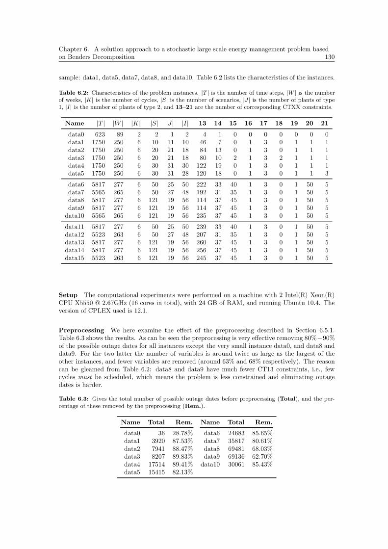
Chapter 6. A solution approach to a stochastic large scale energy management problem basedon Benders Decomposition 130
sample: data1, data5, data7, data8, and data10. Table 6.2 lists the characteristics of the instances.
Table 6.2: Characteristics of the problem instances. |T | is the number of time steps, |W | is the numberof weeks, |K| is the number of cycles, |S| is the number of scenarios, |J | is the number of plants of type1, |I | is the number of plants of type 2, and 13–21 are the number of corresponding CTXX constraints.
Name |T | |W | |K| |S| |J | |I| 13 14 15 16 17 18 19 20 21
data0 623 89 2 2 1 2 4 1 0 0 0 0 0 0 0data1 1750 250 6 10 11 10 46 7 0 1 3 0 1 1 1data2 1750 250 6 20 21 18 84 13 0 1 3 0 1 1 1data3 1750 250 6 20 21 18 80 10 2 1 3 2 1 1 1data4 1750 250 6 30 31 30 122 19 0 1 3 0 1 1 1data5 1750 250 6 30 31 28 120 18 0 1 3 0 1 1 3
data6 5817 277 6 50 25 50 222 33 40 1 3 0 1 50 5data7 5565 265 6 50 27 48 192 31 35 1 3 0 1 50 5data8 5817 277 6 121 19 56 114 37 45 1 3 0 1 50 5data9 5817 277 6 121 19 56 114 37 45 1 3 0 1 50 5data10 5565 265 6 121 19 56 235 37 45 1 3 0 1 50 5
data11 5817 277 6 50 25 50 239 33 40 1 3 0 1 50 5data12 5523 263 6 50 27 48 207 31 35 1 3 0 1 50 5data13 5817 277 6 121 19 56 260 37 45 1 3 0 1 50 5data14 5817 277 6 121 19 56 256 37 45 1 3 0 1 50 5data15 5523 263 6 121 19 56 245 37 45 1 3 0 1 50 5
Setup The computational experiments were performed on a machine with 2 Intel(R) Xeon(R)CPU X5550 @ 2.67GHz (16 cores in total), with 24 GB of RAM, and running Ubuntu 10.4. Theversion of CPLEX used is 12.1.
Preprocessing We here examine the effect of the preprocessing described in Section 6.5.1.Table 6.3 shows the results. As can be seen the preprocessing is very effective removing 80%−90%of the possible outage dates for all instances except the very small instance data0, and data8 anddata9. For the two latter the number of variables is around twice as large as the largest of theother instances, and fewer variables are removed (around 63% and 68% respectively). The reasoncan be gleamed from Table 6.2: data8 and data9 have much fewer CT13 constraints, i.e., fewcycles must be scheduled, which means the problem is less constrained and eliminating outagedates is harder.
Table 6.3: Gives the total number of possible outage dates before preprocessing (Total), and the per-centage of these removed by the preprocessing (Rem.).
Name Total Rem. Name Total Rem.
data0 36 28.78% data6 24683 85.65%data1 3920 87.53% data7 35817 80.61%data2 7941 88.47% data8 69481 68.03%data3 8207 89.83% data9 69136 62.70%data4 17514 89.41% data10 30061 85.43%data5 15415 82.13%

131 6.8. Computational results
Heuristic preprocessing As mentioned earlier, the preprocessing is very effective, but still alarge number of variables remains on certain large instances (data8 and data9) where few cycleshave to be scheduled. For this reason the heuristic conflict detector described as point 5 inSection 6.5.1 is included. As described there the value of α controls the aggressiveness of theheuristic (lower values means more conflicts). We here examine the effect of including the heuristicpreprocessing. The value of α is fixed to 0.05 (for smaller values some instances were infeasible).Table 6.4 shows the results with and without the heuristic given 3600 seconds respectively. Forthis experiment the fuel constraints were added as described for Run 6 in Table 6.6, aggregationwas enabled and postoptimization was disabled. As can be seen, the effect on the final solutionquality is minor for data1–data3, for data4–data5 the solution is improved, while it is worse fordata6, data7, and data10, finally we are now able to provide a solution for data8, which was notpossible earlier.
Table 6.4: Shows the percentage of variables removed (Rem.) and the final solution (Sol.), without theheuristic (No Heur.), and with the heuristic (Heur.) given 3600 seconds respectively. A dash (–) meansno solution could be found, and boldface indicates the best solution found for a given instance.
No Heur. Heur.
Name Rem. Sol. Rem. Sol.
data0 28.78% 8.7371e12 28.78% 8.7371e12data1 87.53% 1.6990e11 87.63% 1.6971e11data2 88.47% 1.4654e11 88.64% 1.4672e11data3 89.83% 1.5537e11 89.92% 1.5578e11data4 89.41% 1.1342e11 89.64% 1.1309e11data5 82.13% 1.3272e11 83.28% 1.3153e11data6 85.65% 9.0945e10 85.72% 9.2508e10data7 80.61% 1.2307e11 80.68% 1.3663e11data8 68.03% – 77.15% 3.2392e12data9 62.70% – 74.13% –
data10 85.43% 1.5303e11 85.44% 1.7455e11
Aggregation Next we examine the effect of aggregation on the solution quality. To that effectthe algorithm is run for 3600 seconds with aggregation enabled and disabled for stage 2 (aggrega-tion is always performed for stage 1). Table 6.5 shows the results, where Vars. is the number ofvariables in the subproblem, Cons. is the number of constraints in the subproblem, and Sol. isthe final solution. For this experiment the fuel constraints were added as described for Run 7 inTable 6.6, heuristic conflicts were included with α = 0.05 and postoptimization was disabled. Ascan be seen the aggregation results in a big reduction in the number of variables and constraintsof the subproblem. For data8, and data10 no solution is found without the use of aggregation.
Fuel constraints We here examine the effect of including the constraints described in Sec-tion 6.6, in an attempt to ensure the feasibility of the subproblem. One can choose to includeeither all the constraints, or only a subset, and to included them only in stage 2 or in both stages.Nine runs are performed, with the settings described in Table 6.6. The results can be seen inTable 6.7. For this experiment heuristic conflicts were included with α = 0.05, aggregation wasenabled and postoptimization was disabled. As can be seen only Run 4, 7 and 10 completes forall the tested instances. Run 10 achieves the best average results.
Postoptimization We here examine the effect of the postoptimization procedure described inSection 6.7.2. For each of the 11 instances three runs are performed, with the number of iterationsrespectively set to 50, 000, 150, 000, and 300, 000. The results can be seen in Table 6.8. For this

Chapter 6. A solution approach to a stochastic large scale energy management problem basedon Benders Decomposition 132
Table 6.5: Effect on final solution of aggregating versus not aggregating in stage 2. Vars. is the numberof variables in the subproblem, Cons. is the number of constraints in the subproblem, and Sol. is thefinal solution. The dash (–) and boldface are as earlier.
Enabled Disabled
Name Vars. Cons. Sol. Vars. Cons. Sol.
data1 5514 8693 1.6971e11 37692 58871 1.6968e11data5 16696 25199 1.3147e11 114346 170849 1.3100e11data7 25898 34181 1.3663e11 529438 686121 1.3412e11data8 41762 48309 3.2392e12 860182 977529 –data10 23150 29457 1.7455e11 469330 581637 –
Table 6.6: Description of the different settings used for the fuel constraint runs
Run Description1 No fuel constraints included2 Fuel constraints (6.44)–(6.47) included in stage 1.3 Fuel constraints (6.44)–(6.47), SI and SII included in stage
1.4 All fuel constraints included in stage 1.5 Fuel constraints (6.44)–(6.47) included in stage 2.6 Fuel constraints (6.44)–(6.47), SI and SII included in stage
2.7 All fuel constraints included in stage 2.8 Fuel constraints (6.44)–(6.47) included in stage 1, SI and
SII included in stage 2.9 Fuel constraints (6.44)–(6.47) included in stage 1, remain-
ing included in stage 2.10 Fuel constraints (6.44)–(6.47), SI and SII included in stage
1, remaining included in stage 2.
experiment the fuel constraints were added as described for Run 10 in Table 6.6, heuristic conflictswere included with α = 0.05. Due to time constraints the previous tests could not be rerun. Ascan be seen there is a clear correlation between the number of postoptimization iterations and thefinal solution quality.
Time We finally examine the solution quality as a function of total time given to the algorithm.Each of the 16 instance is run for respectively 3600 seconds, and 10800 seconds. The resultscan be seen in Table 6.9, and Table 6.10 respectively, where the number in parenthesis is thedeviation from the best known solutions reported on the ROADEF/EURO 2010 challenge website(http://challenge.roadef.org/2010). For the challenge a maximum time of 1800 seconds wasallowed for the first 6 instances, and 3600 seconds for the remaining 10.
As can be seen from the tables, the solution approach performs satisfactorily on instances zeroto five. These were the test instances used in the qualification phase of the contest and are lesscomplicated than the second and third set of instances (data6 to data10, and data11 to data15).For the latter sets, the algorithm runs into difficulty due to the large number of binary variables,particularly for data8 and data9 which are far from the best known solutions, and for data13 whichis not solved at all. Furthermore, formulating and solving the subproblem as an LP and repairingits solution so that it satisfies CT6 and CT12 appears to be an expensive process, despite theaggregation.

133 6.9. Conclusion
Table 6.7: Effect of including fuel constraints. See Table 6.6 for a description of each run. The Avg. rowis the average solution across the instances when all instances were solved. The dash (–) and boldfaceare as earlier.
Name Run 1 Run 2 Run 3 Run 4 Run 5
data 1 1.6986e11 1.6987e11 1.6981e11 1.6986e11 1.6973e11data 5 – 1.2656e11 1.2593e11 1.2707e11 1.3163e11data 7 – 1.3535e11 1.0514e11 1.2517e11 1.3363e11data 8 – – – 2.8047e12 –data10 – 1.3055e11 1.3785e11 1.3667e11 1.1532e11Avg. – – – 6.7269e11 –
Name Run 6 Run 7 Run 8 Run 9 Run 10
data 1 1.6972e11 1.6972e11 1.6987e11 1.6979e11 1.6977e11data 5 1.3039e11 1.3148e11 1.2656e11 1.2654e11 1.2593e11data 7 1.3392e11 1.3663e11 1.4035e11 1.3373e11 1.0563e11data 8 – 3.2393e12 – – 2.1963e12data10 1.5162e11 1.7455e11 1.4273e11 1.6093e11 1.3864e11Avg. – 7.7034e11 – – 5.4725e11
Table 6.8: Effect of postoptimization procedure. The number of iterations for the runs are respectively50, 000, 150, 000, and 300, 000. boldface is as earlier.
Name 50,000 150,000 300,000
data1 1.69711e11 1.69710e11 1.69709e11data5 1.26452e11 1.26453e11 1.26451e11data7 1.10602e11 1.09518e11 1.09013e11data8 2.88400e11 2.79264e11 2.75348e11data10 1.30261e11 1.28788e11 1.28443e11
For the the smaller instances, many of the solutions are repairable, while for the larger instances,there is a lot more variation. It is surprising that for two of the instances where the algorithmperforms poorly (data8 and data13), there is a large number of solutions found but only two arerepairable in one case, while none in the other. Generally it appears that for the larger instances,either the solutions to the master problem can not be adjusted such that they satisfy CT6 andCT12, or the repair algorithm does a poor job.
Doubling the amount of time (Table 6.10) does not significantly change the results and onlydata1, data5, and data6 are improved. The trend of finding many solutions which are non-repairable remain the same.
6.9 Conclusion
In conclusion, we have developed a Benders Decomposition approach to solve the large scale energymanagement problem posed for the ROADEF/EURO 2010 challenge. The approach includesa MIP model of the problem along with additional constraints for ensuring feasibility of thesubproblems, a very effective preprocessing and aggregation scheme, which reduces the size of theproblem significantly, and an algorithm for repairing a solution which only satisfies a subset of theconstraints.
On the first set of instances the approach is competitive, while on the the second two set ofinstances it is not. This is mainly due to the size of the problems, and the time allotted. On the

Chapter 6. A solution approach to a stochastic large scale energy management problem basedon Benders Decomposition 134
Table 6.9: Results for different problem instances given 3600 seconds. The following information isshown: the number of optimality cuts added (#Cuts), the number of solutions found in stage 2 (#Sols),the number of solutions found in stage 2 that were repairable (#Rep), the solution value (Sol.), thepercentage deviation from the best known solution (#Dev), and the average deviation for the three testsets of respectively six, five and five instances (#Avg).
Name #Cuts #Sols. #Rep. Sol. Dev. Avg.
data0 5 2517 2517 8.7372e12 0.0709%data1 6 352 312 1.6971e11 0.1008%data2 17 82 82 1.4629e11 0.1639%data3 14 86 86 1.5475e11 0.2050%data4 23 36 35 1.1206e11 0.4157%data5 21 38 37 1.2645e11 0.4997% 0.2427 %
data6 14 12 12 9.0113e10 8.0173%data7 5 121 1 1.0901e11 34.2953%data8 3 1486 2 2.7535e11 236.0938%data9 9 7 3 3.5103e12 4193.8891%data10 37 7 5 1.2844e11 62.3461% 906.9283 %
data11 61 447 11 8.8464e10 14.0143%data12 20 12 12 8.8135e10 15.2850%data13 16 1017 0 – –%data14 10 8 4 1.0092e11 32.4820%data15 46 35 2 1.5758e11 109.8220% 42.9008%
Table 6.10: Results for different problem instances given 10800 seconds. The information given is as forthe previous table.
Name #Cuts #Sols. #Rep. Sol. Dev. Avg.
data0 5 2517 2517 8.7372e12 0.0709%data1 6 872 583 1.6971e11 0.1007%data2 17 153 153 1.4629e11 0.1639%data3 14 165 165 1.5475e11 0.2050%data4 23 73 72 1.1206e11 0.4156%data5 21 76 74 1.2643e11 0.4842% 0.2401 %
data6 14 23 23 8.9659e10 7.4733%data7 5 481 22 1.0901e11 34.2953%data8 3 4292 2 2.7535e11 236.0938%data9 9 12 10 3.5103e12 4193.8891%data10 37 10 9 1.2844e11 62.3461% 906.8179 %
data11 61 458 22 8.8464e10 14.0143%data12 20 25 25 8.8135e10 15.2850%data13 16 2187 0 – –%data14 10 118 8 1.0092e11 32.4820%data15 46 126 2 1.5758e11 109.8220% 42.9008%
second set of instances and 5 blind instances we placed 14th out of 19 teams in the final of thecompetition. Being one of the few optimal methods proposed, it was unable to compete with theheuristics given only 3600 seconds of computing time. The sophisticated approach can, however,provide information as to the quality of solutions through the lower bound information which can

135 Bibliography
be obtained at each iteration of the Benders algorithm as well as insights into the structure onthe problem.
Bibliography
Benders, J. F. Partitioning procedures for solving mixed variables programming problems. Nu-merische Mathematik, 4:238 – 252, 1962.
Cabero, J., Ventosa, M. J., Cerisola, S., Alvaro Baıllo. Modeling risk management in oligopolisticelectricity markets: A benders decomposition approach. IEEE Transactions on power systems,25(1):263 – 271, 2010.
Canto, S. P. Application of benders decomposition to power plant preventive maintenance schedul-ing. European Journal of Operational Research, 184:759 – 777, 2008.
Contreras, I., Cordeau, J.-F., Laporte, G. Benders decomposition for large scale uncapacitatedhub location. Technical Report CIRRELT-2010-26, Interuniversity research centre on enterprisenetworks, logistics, and transportation, 2010.
Guyon, O., Lemaire, P., Pinson, E., Rivreau, D. Cut generation for an integrated employeetimetabling and production scheduling problem. European Journal of Operational Research,201:557 – 567, 2010.
Mercier, A., Cordeau, J.-F., Soumis, F. A computational study of benders decomposition for theintegrated aircraft routing and crew scheduling problem. Computers and Operations Research,32:1451 – 1476, 2005.
Naoum-Sawaya, J., Elhedhli, S. A nested benders decomposition approach for telecommunicationnetwork planning. Naval Research Logistics, 57:519 – 539, 2010.
Porcheron, M., Gorge, A., Juan, O., Simovic, T., Dereu, G. Challenge roadef/euro2010 : A large-scale energy management problem with varied constraints.http://challenge.roadef.org/2010/sujetEDFv22.pdf, 2009.
Santos, T. N., Diniz, A. L. Feasibility and optimality cuts for the multi-stage benders decompo-sition approach: Application to the network constrained hydrothermal scheduling. In Power &Energy Society General Meeting, 2009. PES ’09. IEEE, 2009.
Wu, L., Shahidehpour, M. Accelerating the benders decomposition for network-constrained unitcommitment problems. Energy Systems, 1:339 – 376, 2010.

Bibliography 136

Chapter 7
A hybrid Adaptive Large Neighborhood
Search heuristic for lot-sizing with setup
times
Laurent Flindt Muller Simon Spoorendonk David Pisinger
Department of Management Engineering,Technical University of Denmark
Produktionstorvet, Building 426, DK-2800 Kgs. Lyngby, [email protected], [email protected], [email protected]
Abstract This paper presents a hybrid of a general heuristic framework and a general purpose mixed-
integer programming (MIP) solver. The framework is based on local search and an adaptive procedure
which chooses between a set of large neighborhoods to be searched. A mixed integer programming solver
and its built-in feasibility heuristics is used to search a neighborhood for improving solutions. The general
reoptimization approach used for repairing solutions is specifically suited for combinatorial problems where
it may be hard to otherwise design suitable repair neighborhoods. The hybrid heuristic framework is
applied to the multi-item capacitated lot sizing problem with setup times, where experiments have been
conducted on a series of instances from the literature and a newly generated extension of these. On average
the presented heuristic outperforms the commercial MIP solver ILOG CPLEX and the best heuristics from
the literature. Furthermore, we improve the best known upper bounds on 60 out of 100 and improve the
lower bound on all 100 instances from the literature.
Keywords: Adaptive large neighborhood search, capacitated lot sizing problem with setup times
7.1 Introduction
The adaptive large neighborhood search (ALNS) heuristic is a concept introduced by Røpke andPisinger (2006). The ALNS heuristic is a large neighborhood improvement heuristic that operateson top of a construction heuristic. The improvement is done using a local search method, e.g.,simulated annealing or tabu search, choosing between different neighborhoods. In each iteration ofthe search a destroy neighborhood is chosen to destroy the current solution, and a repair neighbor-hood is chosen to repair the solution. The neighborhoods are weighted according to their successand weights are adjusted as the ALNS heuristic progresses. Destroy and repair neighborhoods arenormally assumed to be searched by fast heuristics.
The main motivation for extending the ALNS heuristic to a hybrid version is, that not allproblem types are equally well suited for defining neighborhoods. Especially the constructionand the exploration of repair neighborhoods can be a challenge, both with respect to finding ameaningful repair operation and testing feasibility of such an operation. To address this problem,
137

Chapter 7. A hybrid Adaptive Large Neighborhood Search heuristic for lot-sizing with setuptimes 138
we propose to use a mixed integer programming (MIP) solver in the repair phase of the ALNSheuristic. The idea is to solve a restricted subproblem that is based on a partial solution wherevariables are fixed (or bounded). The process of constructing a subproblem, and the followingreoptimization of the subproblem with the use of a MIP solver, can in the context of an ALNSheuristic be seen as the application of a destroy and a repair neighborhood. As such the hybridALNS can be viewed as a specialization of the ALNS framework which simplifies the task ofdefining repair neighborhoods.
The reoptimization of of the subproblems done in the repair neighborhoods relies heavily onprimal heuristics in the MIP solver to produce good upper bounds since it may be too cumbersometo solve the subproblem to optimality. Heuristics found in modern MIP solvers include the localbranching heuristic by Fischetti and Lodi (2003), the feasibility pump introduced by Fischettiet al. (2005) and refined by Bertacco et al. (2007); Achterberg and Berthold (2007), and therelaxation induced neighborhood search by Danna et al. (2005). Naturally such MIP heuristicsare constructed in such a way that they can be applied directly to a problem without taking intoaccount special characteristics. Also, the MIP heuristics are limited in the sense that they are onlyapplied within the branch-and-bound tree and are induced from the current fractional solution.The hybrid ALNS works with different neighborhoods, outside the scope of a branch-and-boundtree, and takes historical information into account.
The ALNS framework by Røpke and Pisinger (2006) has grown out of the large neighborhoodsearch framework by Shaw (1998). The heuristic has several similarities with variable neighbor-hood search, see e.g., Mladenovic and Hansen (1997), and hyper-heuristics, see e.g., Burke et al.(2003). However, there are no adaptiveness built into the basic idea of the variable neighborhoodsearch. This approach mainly relies on the diversity of the neighborhoods being used. The hyper-heuristic approach operates on simpler low-level heuristics whereas the ALNS heuristic operates onneighborhoods. Furthermore, an evaluation function is used to calculate a score for each low-levelheuristic, based on which the best scoring heuristics is chosen for the next iteration. The ALNSheuristic uses a random selection between all weighted neighborhoods to choose a neighborhood forthe next iteration. This allows for bad performing neighborhoods to be chosen occasionally, whichincreases the search diversity. ALNS heuristics have been implemented for vehicle routing prob-lems with great success, see Røpke and Pisinger (2006); Pisinger and Røpke (2007). Examples ofan application of the framework outside a routing problem context are few: Cordeau et al. (2010)schedule technicians and tasks in a telecommunications company and Muller (2009) presents anALNS heuristic for the resource-constrained project scheduling problem. For a recent survey onlarge neighborhood search and the ALNS framework we refer to Pisinger and Røpke (2010).
The lot sizing problem (LSP) with setup times and setup costs can be defined as follows: Givenone resource, schedule the production of a set of items over a given number of time periods suchthat all demands of items are met, and such that the capacity of the resource is not exceeded.The production of an item and each setup of production consumes capacity on the resource andhas a cost. The difference between setup times and setup costs, is that setup times consumes anamount of capacity on the resource, while setup costs is an extra cost incurred in the objectivefunction. The LSP with setup times and setup costs is NP-hard, see e.g., Pochet and Wolsey(2006). Maes et al. (1991) show that the problem remains NP-hard for the case with no setupcosts (in fact just finding a feasible solution is NP-hard). Heuristics for the LSP with setup timesand setup costs include the tabu search heuristic of Gopalakrishnan et al. (2001), the variableneighborhood search heuristic of Hindi et al. (2003), and the cross entropy-Lagrangian hybridheuristic of Caserta and Rico (2009). For some comparisons see for instance Jans and Degraeve(2007) or Buschkuhl et al. (2010). Exact approaches for the LSPST with setup times and setupcosts include branch-and-cut algorithms by Belvaux andWolsey (2000); Wolsey (2002); Miller et al.(2000) and a branch-and-price algorithm by Degraeve and Jans (2007). The good performance ofthe branch-and-cut algorithms suggest that using a MIP solver to solve restricted subproblems ofthe LSP with setup times and setup costs can be done in reasonable time.
A recent study by Sural et al. (2009) shows that the standard benchmark instances of Trigeiroet al. (1989) are considerably harder when setup costs are removed. Furthermore, Sural et al.(2009) consider an extension of the standard (heterogeneous) instances denoted the homogeneous

139 7.2. A hybrid ALNS algorithm
instances where all holding costs are equal. Their experiments showed that the homogeneousinstances have even larger integrality gaps than the heterogeneous instances. It is thus of interestto develop heuristics for the case with setup times and no setup costs, and this is the problemconsidered in the following. Papers relating to the LSP with setup times and no setup costs includethe MIP based heuristic of Denizel and Sural (2006), and the Lagrangian heuristic of Sural et al.(2009). In the following we will refer to the LSP with setup times and no setup costs as theLSPST.
The contribution of this paper is an ALNS heuristic which combines the strengths of modernMIP solvers with the diversity of the ALNS heuristic, creating a “hybrid” approach. The repairneighborhoods employ the MIP solver in a generic fashion and neighborhoods are thus applicableto a large variety of problems. An evaluation of the hybrid ALNS heuristic is applied to theLSPST, on a set of instances found in the literature. The ALNS algorithm outperforms ILOGCPLEX and the current best heuristic of Sural et al. (2009) both with respect to the quality ofsolutions and lower bounds. During the experiments we found 60 new best upper bounds (forthe 100 instances also considered by Sural et al. (2009)), and improved all lower bounds. Thisindicates the usefulness of the hybrid ALNS approach.
The paper is organized as follows: Section 7.2 gives an outline of the ALNS framework anddescribes the hybrid variant proposed in this paper, Section 7.3 presents an application of thehybrid ALNS heuristic to the LSPST, and Section 7.4 contains the experimental results performedon the instances of Sural et al. (2009) which is an extension of the instances of Trigeiro et al. (1989),and on a new set of larger instances. Section 7.5 concludes the paper and suggest new directionsfor future research.
7.2 A hybrid ALNS algorithm
We begin with an outline of the ALNS framework as described by Pisinger and Røpke (2007).The framework is divided into three parts, i) a master local search framework, ii) a set of largeneighborhoods that either destroy for a solution or repair a for a partial solution, and iii) aprocedure for choosing neighborhoods which adapts based on historical information. Followingthis we present the hybrid ALNS algorithm.
At the top level (also denoted master level) any local search heuristic can be applied, e.g.,simulated annealing, tabu search, guided local search, or GRASP (greedy randomized adaptivesearch procedure). A neighborhood of a solution is a set of solutions obtained by performing someoperation on the original solution. In large neighborhoods these operations involve changing severalsettings in the solution at once leading to a neighborhood of potentially exponential size. Theprocedure for choosing neighborhoods can be pictured as a roulette wheel spinning and randomlychoosing a neighborhood. The weights of all neighborhoods are updated based on historicalsuccess. Hence, successful neighborhoods have a higher probability to be used as time passes,although all neighborhoods have a small chance of being chosen to ensure diversity.
The ALNS framework can be described as follows: Given a starting solution, the heuristiciteratively tries to improve it. The set of neighborhoods is divided into destroy neighborhoodsN− and repair neighborhoods N+. Given a current solution x a destroy neighborhood n− ∈N− performs an operation on x, stores the removed elements in an item bank B and leaves apartial solution x. A repair neighborhood inserts elements from the item bank into x creatinga new solution x′. In the case of the hybrid ALNS heuristic presented in this paper, the repairneighborhoods make use of a MIP solver. A roulette wheel for each of the sets N− and N+ is usedin each iteration to choose which destroy and which repair neighborhood should be used. This isbased on a weight π for each neighborhood that is initialized at the beginning according to thequality of the neighborhood (this is a user defined consideration to be made a priori). During thelocal search the weights are updated according to the quality of the solutions produced with thegiven neighborhoods. The motivation behind this is, that not all neighborhoods perform equallywell on all problem instances – hence the weights of the neighborhoods adapt to the instanceduring the execution of the algorithm and hopefully produce better solutions overall.

Chapter 7. A hybrid Adaptive Large Neighborhood Search heuristic for lot-sizing with setuptimes 140
ALNS
1 x is an initial solution; set x∗ := x2 repeat3 Choose n− ∈ N− and a n+ ∈ N+ based on π4 Generate solution x′ based on x, n−, and n+
5 if x′ is accepted6 then x := x′
7 if x′ < x∗
8 then x∗ := x′
9 Update π for N− and N+
10 until stop criteria is meet11 return x∗
Figure 7.1: Pseudo-code overview of the ALNS framework.
As mentioned above, the weights of the neighborhoods are updated according to how successfula neighborhood is in obtaining better and new solutions. In the paper by Pisinger and Røpke (2007)the weights are updated after certain given time segments and the weight of a neighborhood isbased on the observed weight πi,t of neighborhood i at time segment t which in each iteration isincremented with values dependent on the quality of the new solution x′.
At the end of a time segment a smoothened weight πi,t is calculated for use in the roulettewheel. This is based on πi,t and a reaction factor r which indicates how much the roulette weightdepends on previous success. Previous success is calculated as the observed weight πi,t dividedby the number of times ai,t neighborhood i has been chosen in time segment t. The updatedsmoothened weight is:
πi,t+1 = rπi,t
ai,t+ (1− r)πi,t.
A low reaction factor keeps the weight at about the same level during the algorithm. A neighbor-hood i has the probability:
pt(i) =πi,t
∑
j∈N πj,t
of being chosen in time segment t.In Figure 7.1, the pseudo-code is given for the ALNS framework. The criteria for accepting a
new solution in line 5 depends on the choice of local search framework and the score update online 9 can be performed using different strategies. The choices made for the hybrid ALNS heuristicwill be described in the following sections.
The basic idea behind the proposed hybrid ALNS heuristic is, that instead of designing specialpurpose repair neighborhoods, which may not always be straight forward, we use a MIP solver inorder to repair (or reoptimize) a solution. The destroy neighborhood either explicitly or implicitlyselects a number of variables from the MIP model. A MIP based repair neighborhood then createsa subproblem of the original problem where the selected variables are “free” in the sense that noadditional constraints are imposed on these variables, while the remaining variables are either fixedor bounded based on their values in the current solution. Thus the MIP based repair neighborhoodwill in effect search a neighborhood around the current solution. Using a MIP solver as a repairneighborhood provides an easy tool to calculate lower bounds during the search. We propose,that when an improved solution is found, the root node of the MIP is resolved with all variablesunfixed, and the current solution as an initial upper bound. For modern MIP solvers an initialupper bound is used for both pre-processing and reduced cost fixing during the optimization.Hence, a good initial upper bound may yield improved lower bounds compared to solving the rootnode with no (or a bad) initial solution. This way, the ALNS heuristic can provide valid lowerbounds and an estimation of the solution quality based on the integrality gap.

141 7.3. An application of ALNS to the LSPST
7.3 An application of ALNS to the LSPST
In this section we present an application of the hybrid ALNS heuristic to the LSPST. First,a description of the mathematical model is given, then the master level local search procedureis presented, next a description if an adjusted weight calculation method used in the adaptiveprocedure is given, followed by a description of the neighborhoods employed, and finally theparameter values are presented.
7.3.1 Problem description
This section briefly presents the traditional mathematical formulation (see e.g., Belvaux andWolsey (2000)) of the LSPST. Let I = {1, . . . , n} be the set of items and T = {1, . . . ,m} bethe set of time periods. The data set is given as follows: hi
t ≥ 0 is the unit inventory cost of item iat time t, dit ≥ 0 is the demand of item i at time t, αi
t ≥ 0 is the capacity used for producing itemi at time t, βi
t ≥ 0 is the capacity used for setting up the production of item i at time t, Ct ≥ 0is the capacity of the resource at time t, and M is a sufficiently large constant. The variables aregive as follows: si0 is the number of units of item i in the initial inventory, sit is the number ofunits of item i in stock after time t, xi
t is the number of units of production of item i at time t,and yit indicates if a setup for production of item i at time t has been done. All variables exceptthe y-variables are positive continuous variables. The y-variables are binary and force the othervariables to attain integer values (if all constants are also integer). The mathematical model forthe LSPST:
min∑
i∈I
(
hi0s
i0 +
∑
t∈T
hits
it
)
(7.1)
s.t. sit−1 + xit = dit + sit t ∈ T, i ∈ I (7.2)
xit ≤Myit t ∈ T, i ∈ I (7.3)∑
i∈I
(
αitx
it + βi
tyit
)
≤ Ct t ∈ T (7.4)
sit, s0t , x
it ≥ 0, yit ∈ B t ∈ T, i ∈ I (7.5)
The objective (7.1) is to minimize holding cost. Constraints (7.2) ensure flow conservation of theitem. That is, items in stock plus the items produced in a time period must equal the numberof items demanded in this time period plus the number of items in stock after this time period.Constraints (7.3) ensure that production of an item can only occur if the resource is set up toproduce that item. Constraints (7.4) guarantee that the production and setup capacity usagescannot exceed the resource capacity. The domains of the variable are specified by constraints(7.5).
7.3.2 Local search
In this paper steepest descent has been chosen as the local search procedure. Because the destroyneighborhoods merely unfixe parts of the variables, and because the MIP repair neighborhoodsuse the current solution as an initial upper bound, it is always possible for the MIP solver tofind that solution again. Therefor, the MIP solver never returns a solution that is worse than thecurrent one. Hence, a selection process for choosing worse solutions would not apply.
To diversify the search, the search is restarted at different solutions when no improvementshave occurred in a number of iterations (chosen to be equal to the segment size for updatingthe neighborhood weights). For the initial restart the second best solution is chosen (the currentsolution is the best solution). In subsequent restarts, the local search either switches back tothe best solution if it is not the current one or switches to the next best solution that has notpreviously been used for a restart. The reason for returning to the best solution in an attempt

Chapter 7. A hybrid Adaptive Large Neighborhood Search heuristic for lot-sizing with setuptimes 142
to find further improvements is that the neighborhoods may have obtained different scores in themeantime yielding a diversified exploration of the neighborhood of that solution.
To speed up the subproblem solution process, we suggest to limit the number of exploredbranch nodes or end the search after a given time limit. MIP heuristics are applied in the MIPsolver to obtain feasible solutions rapidly.
7.3.3 Adaptive weight adjustments
In this paper a slightly different approach, compared to the fixed scoring scheme of Røpke andPisinger (2006); Pisinger and Røpke (2007), is used for updating the observed weights. Thereason for this is the choice of local search procedure. For the selected procedure, a solution isonly accepted when it is better than the current solution, which may result in long periods withoutany accepted solutions. If a fixed scoring scheme was used all neighborhoods would score equallybad, while for the employed scheme it is possible to differentiate the neighborhoods that producesolutions which are almost as good as the current one and the ones that produce solutions whichare far worse. Let cx be the objective value of the current solution and let cx′ be the objectivevalue of the new solution. The observed weight πi,t of neighborhood i at time segment t is updatedas follows
πi,t = πi,t + k(cx−cx′)/cx
where k is some constant.
7.3.4 Destroy neighborhoods
Except for the random removal neighborhood each neighborhood focuses on specific structuralproblems in a solution to the LSPST, e.g., too many items in stock, or an often changing productionof items. A parameter Q controls how large a part of the current solution is destroyed. It ismeasured in a percentage of combined production for the LSPST. The destroy neighborhoodsare divided in two steps: i) a removal candidate set, R, of sets of production variables, i.e., setsof x-variables, is constructed based on the chosen destroy neighborhood, ii) iteratively a set ofproduction variables from R are selected for removal until production corresponding to Q hasbeen unfixed, or no more sets of variables remain. Depending on the destroy neighborhood chosenthese variables are either randomly selected or randomly selected based on some weight. Let inthe following (x, y, s) denote the current solution.
Random. Unfixes production variables at random throughout the production plan:
R ={
{xit} : xi
t > 0, t ∈ T, i ∈ I}
.
Variable from R are chosen randomly. The neighborhood is good at diversing the search,and is useful if the search is stuck in a local minimum.
Production causing stock. Unfixes production variables that causes items to be placed instock. Hopefully, the production can be inserted at a later time in the production plan,hence saving inventory expenses:
R ={
{xit} : sit > 0 ∨ sit+1 > 0, t ∈ T, i ∈ I
}
.
Variables from R are chosen randomly.
Capacity critical. Unfixes production of items in time steps, where some resource is fully loaded.This allows for a reshuffling of the production:
R ={
{xit} : xi
t∗ > 0 ∧ (t = t∗ ∨ t = t∗ − 1 ∨ t = t∗ + 1), i ∈ I}
,
where t∗ = argmax{∑I xit : t ∈ T }, i.e., t∗ is the time period with the most combined
production. Variables for time steps preceding and following t∗ are included to open thepossibility of shifting the production between these time periods. Variables from R areunfixed randomly.

143 7.3. An application of ALNS to the LSPST
Stocked items. Unfixes production of items that have the largest amount of units in stockthroughout the production plan. The idea is to attempt a reshuffle of stocked items be-tween those types of items that are favorable to put in stock, e.g., due to low holding cost:
R =
{
{xit : t ∈ T } :
∑
t∈T
sit > 0, i ∈ I
}
Sets of variables from R are chosen randomly, where each set S ∈ R corresponding to someitem i∗ has weight
∑
t∈T si∗
t . A minimum of two item types are unfixed.
Time periods with high stock density. Unfixes production from time periods where manyitems are in stock. The idea is to reshuffle the production (and thereby the stocked items)into the previous or succeeding time periods. The time periods are sorted according to thenumber of stocked items. When the production in a time period is cleared, the time periodbefore and after are also cleared:
R ={
{xit−1, x
it, x
it+1 : i ∈ I} : t ∈ T
}
Sets of variables from R are chosen randomly, where each set S ∈ R corresponding to sometripe of time (t∗ − 1, t∗, t∗ + 1) has weight
∑
i∈I(sit∗−1 + sit∗ + sit∗+1).
Production higher than demand. When there are productions that are very high comparedto the demand of the corresponding item in the time period, a lot of items are put in stock.Often a solution can be shifted, such that the majority of the production is moved to thefollowing time period:
R ={
{xit−1, x
it, x
it+1} : t ∈ T, i ∈ I
}
Sets of variables from R are chosen randomly, where each set S ∈ R corresponding to someitem i∗ and some triple of time (t∗ − 1, t∗, t∗ + 1) has weight xi∗
t∗ − di∗
t∗ .
7.3.5 Repair neighborhoods
The MIP repair neighborhoods employed for the LSPST are:
Bound by solution value. Bound non-unfixed variables x to a fraction of their current value,i.e., if xi
t is a variable which has not been unfixed by a destroy neighborhood, fix xit ≥ δxi
t
for δ ∈ [0, 1]. In this paper δ = 0.5 was chosen. Production variables x imply the setupvariables y. Hence, whenever xi
t > 0 we bound the variable ytt = 1. Stock is generally tobe avoided, therefor we fix all lower bounds of the stock variables s to 0 so that we do notaccidentally force unnecessary stock.
Fix by solution value. Fix non-unfixed variables x, to their value in the current solution, whereproduction equals demand, i.e., we fix xi
t = xit where we have xi
t = dit. In solutions for theLSPST, this scenario happens frequently in consecutive time periods for the production ofan item. In order to allow some diversification in the production we only fix productionwhen there is no stock in the preceding nor the succeeding item periods, i.e., we do notfix the production in the first and the last time period in consecutive time periods, whereproduction equals demand for a certain item.
7.3.6 ALNS parameters
A time limit used at the master level of 300 seconds is chosen as the termination criteria of thesteepest descent local search. The reaction factor r is set fairly high at 0.8 since we expect fewiterations, and therefor would like the neighborhood weights to converge fast. All neighborhoodsare initialized with a weight of 1. During the first iteration, an estimate of the overall number ofiterations is calculated based on the running time of that iteration. The segment size for updating
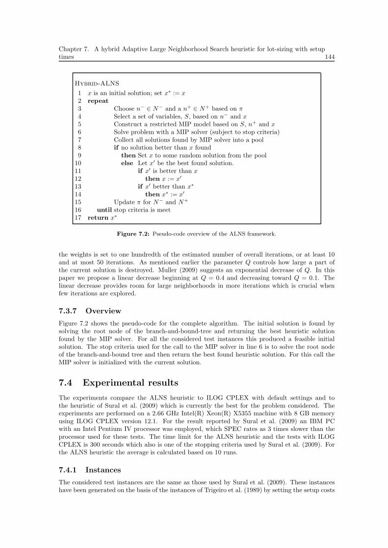
Chapter 7. A hybrid Adaptive Large Neighborhood Search heuristic for lot-sizing with setuptimes 144
Hybrid-ALNS
1 x is an initial solution; set x∗ := x2 repeat3 Choose n− ∈ N− and a n+ ∈ N+ based on π4 Select a set of variables, S, based on n− and x5 Construct a restricted MIP model based on S, n+ and x6 Solve problem with a MIP solver (subject to stop criteria)7 Collect all solutions found by MIP solver into a pool8 if no solution better than x found9 then Set x to some random solution from the pool
10 else Let x′ be the best found solution.11 if x′ is better than x12 then x := x′
13 if x′ better than x∗
14 then x∗ := x′
15 Update π for N− and N+
16 until stop criteria is meet17 return x∗
Figure 7.2: Pseudo-code overview of the ALNS framework.
the weights is set to one hundredth of the estimated number of overall iterations, or at least 10and at most 50 iterations. As mentioned earlier the parameter Q controls how large a part ofthe current solution is destroyed. Muller (2009) suggests an exponential decrease of Q. In thispaper we propose a linear decrease beginning at Q = 0.4 and decreasing toward Q = 0.1. Thelinear decrease provides room for large neighborhoods in more iterations which is crucial whenfew iterations are explored.
7.3.7 Overview
Figure 7.2 shows the pseudo-code for the complete algorithm. The initial solution is found bysolving the root node of the branch-and-bound-tree and returning the best heuristic solutionfound by the MIP solver. For all the considered test instances this produced a feasible initialsolution. The stop criteria used for the call to the MIP solver in line 6 is to solve the root nodeof the branch-and-bound tree and then return the best found heuristic solution. For this call theMIP solver is initialized with the current solution.
7.4 Experimental results
The experiments compare the ALNS heuristic to ILOG CPLEX with default settings and tothe heuristic of Sural et al. (2009) which is currently the best for the problem considered. Theexperiments are performed on a 2.66 GHz Intel(R) Xeon(R) X5355 machine with 8 GB memoryusing ILOG CPLEX version 12.1. For the result reported by Sural et al. (2009) an IBM PCwith an Intel Pentium IV processor was employed, which SPEC rates as 3 times slower than theprocessor used for these tests. The time limit for the ALNS heuristic and the tests with ILOGCPLEX is 300 seconds which also is one of the stopping criteria used by Sural et al. (2009). Forthe ALNS heuristic the average is calculated based on 10 runs.
7.4.1 Instances
The considered test instances are the same as those used by Sural et al. (2009). These instanceshave been generated on the basis of the instances of Trigeiro et al. (1989) by setting the setup costs

145 7.4. Experimental results
Group Instances – Homogeneous Instances – Heterogeneous
SE G53, G54, G51-10–G58-10, G66-10–G72-10,G74-10, G66-15, G69-15, G71-15 (21 in-stances)
G51–G56, G59, G51-10–G60-10, G66-10–G75-10, G66-15, G67-15, G69-15–G71-15,G74-15 (33 instances)
SH G51, G52, G55–G60, G66–G75, G59-10, G60-10,G73-10, G75-10, G67-15, G68-15, G70-15,G72-15–G75-15 (29 instances)
G57, G58, G60, G66–G75, G68-15, G72-15,G73-15, G75-15 (17 instances)
ME – G54-30, G54-45 (2 instances)
MH G51-30–G60-30, G51-45–G60-45, G66-60–G75-60, G66-90–G75-90 (40 instances)
G51-30–G53-30, G55-30–G60-30, G51-45–G53-45, G55-45–G60-45, G66-60–G75-60,G66-90–G75-90 (38 instances)
Table 7.1: The division of the instances in easy and hard groups for respectively the heterogeneous andthe homogeneous instances.
to 0, and setting all zero demand to two. The base set of Trigeiro et al. (1989) are divided intofour groups: the five instances G51–G55 each has 12 items and 15 time periods, the five instancesG56–G60 each has 24 items and 15 time periods, the five instances G66–G70 each has 12 items and30 time periods, and the five instances G71-G75 each has 24 items and 30 time periods. In additionto these instances, Sural et al. (2009) generate four new groups having 10 time periods and twonew groups having 15 time periods by taking the original instances and reducing the number oftime periods to respectively 10 and 15. These are in the following denoted by appending -10 and-15 to the name of the original instance. This results in 50 heterogeneous instances. Additional50 homogeneous instances were created by Sural et al. (2009) on the basis of the heterogeneousinstances by setting all holding costs to 1.
In order to experiment with larger (and harder) instances, we have generated a number of newinstances in a similar way as Sural et al. (2009): For each of the original instances containing 15time periods an instance containing respectively 30 and 45 time periods is created by concatenatingthe 15 time period instance (two respectively three times). Likewise, for each of the originalinstances containing 30 time periods, an instance containing respectively 60 and 90 time periods iscreated by concatenation. These are in the following denoted by appending -30, -45, -60 and -90
to the name of the original instance. Again, a further set of homogeneous instances is created onthe basis of these by setting all holding costs to 1. This results in a total of 40 new heterogeneousand 40 new homogeneous instances. The total number of instances considered is thus 180.
During the conducting of the experiments, we observed that some instances appeared to beharder than others. In order to better evaluate the performance of the ALNS heuristic, we dividethe instances into: hard and easy based on the following criteria: if ILOG CPLEX could not solvethe instance to optimality within 300 seconds the instance is hard, otherwise it is easy. The hardand easy groups are again divided into two, one containing the instances of Sural et al. (2009),the other containing the new instances created here. The group of easy and hard instances fromSural et al. (2009) is in the following denoted SE and SH respectively, and the group of easy andhard instances generated for this paper is denoted ME an MH respectively. Table 7.1 shows theresulting groups and the instances they contain.
7.4.2 Comparison
Table 7.2 shows a comparison of the results obtained by applying the ALNS heuristic, defaultILOG CPLEX, and the best heuristic of Sural et al. (2009) (SDW) to the benchmark instances.The results are shown as an average of over the instances in the groups divided by easy andhard, and heterogeneous and homogeneous. Detailed results for each instance can be found inAppendix 7.A.
When considering the instances of Sural et al. (2009), we see that both the ALNS heuristicand the MIP solver outperforms the best heuristic (SDW) of Sural et al. (2009). Taking the bestupper and lower bounds found by either the ALNS heuristic or the MIP solver we find 24 new best

Chapter 7. A hybrid Adaptive Large Neighborhood Search heuristic for lot-sizing with setuptimes 146
ALNS MIP Sural et al. (SDW)
Group LB UB UB∗ gap Time(s) LB UB gap Time(s) LB UB gap Time(s)
SE 15.57 0.09 0.00 20.06 13.05 0.00 0.00 0.00 6.69 23.68 0.17 37.09 3.70
11.78 0.02 0.00 28.17 18.02 0.00 0.00 0.00 9.25 15.95 2.28 24.59 5.73
SH 11.86 0.25 0.01 14.75 101.65 12.36 0.52 33.37 216.57 14.69 0.96 21.04 12.82
11.88 0.32 0.02 15.07 135.48 13.77 0.53 41.95 248.24 15.24 4.32 27.28 24.59
SE+SH 13.42 0.18 0.01 16.98 64.44 7.17 0.30 19.36 128.42 18.46 0.63 27.78 8.99
11.81 0.12 0.01 23.71 57.96 4.68 0.18 14.26 90.51 15.71 2.98 25.51 12.14
ME - - - - - - - - - - - - -3.53 0.00 0.00 3.65 25.23 0.00 0.00 0.00 1.54 - - - -
MH 15.44 0.67 0.07 20.40 229.50 20.57 1.29 161.75 264.18 - - - -12.12 1.16 0.28 16.18 243.44 17.83 1.25 148.21 274.73 - - - -
ME+MH 15.44 0.67 0.07 20.4 229.50 20.57 1.29 161.75 264.18 - - - -11.69 1.10 0.27 15.56 232.53 16.93 1.18 140.8 261.07 - - - -
All 14.32 0.40 0.04 18.50 137.80 13.12 0.74 82.64 188.76 - - - -11.76 0.56 0.12 20.09 135.54 10.13 0.63 70.50 166.31 - - - -
Table 7.2: Comparison of the ALNS heuristic with default ILOG CPLEX and the SDW heuristic of Suralet al. (2009). The LB column is the average deviation in percent of the lower bound from the best foundsolution across all runs calculated as UB − LB/UB, thus smaller is better. The UB column is likewisethe average deviation of the upper bound form the best found solution, the UB∗ column is the best foundsolution solution found across the 10 runs of the ALNS heuristic. The gap column is the average integralitygap in percent at the point where the procedure stops, and the Time column is the average time usedto find the best solution for the ALNS heuristic and the MIP solver, and for the heuristic of Sural et al.(2009) it is the total times reported in that paper. For the ALNS heuristics the results are reported asaverage of 10 runs. For each class the upper line are the homogeneous results and the lower line are theheterogeneous results. For each line the best value across the algorithms are indicated in boldface.
upper bounds and 50 new best lower bounds (out of 50) for the homogeneous instances, and 36new best upper bounds and 50 new best lower bounds (out of 50) for the heterogeneous instances(see the next section for details). Considering only the SE instances, the MIP solver outperformsthe ALNS heuristic on all parameters which is not surprising since optimality is proved. However,for the SH instances the roles are reversed, and the ALNS heuristic outperforms the MIP solveron all parameters. Taking the combined results for the SE and SH instances the ALNS producesthe best upper bounds and uses less time compared to ILOG CPLEX to find the best solutionsbut the MIP solver produces the best lower bounds. On the homogeneous instances the ALNSheuristic produces the best average gaps, while for the heterogeneous it is the MIP solver. Tobe fair it must be noted that the heuristic of Sural et al. (2009) is by far fastest on average eventhough it produces much worse solutions.
Next, considering the instances generated for this paper we see that for the ME instancesthe ALNS heuristic and the MIP solver tie for the upper bound, while the MIP solver is betterwith respect to lower bounds, gaps, and time to find best solutions. For the hard instancesthe ALNS heuristic outperforms the MIP solver on all parameters for both homogeneous andheterogeneous instances. Taking the combined results for the ME and MH instances, the ALNSheuristic outperforms the MIP solver on all parameters.
Finally, considering all the instances together we see that the ALNS heuristic outperforms theMIP solver on all parameters except for the lower bounds, producing upper bounds which are onaverage about 46% better than the MIP solver on the homogeneous instances, and on averageabout 11% better than the MIP solver on the heterogeneous instances.
7.5 Conclusion
We have presented a hybrid heuristic solution approach based on the ALNS framework where aMIP solver is used in the repair phase. This results in a general hybrid ALNS algorithm where i)

147 7.A. Detailed results
Instance ALNS MIPLB UB UB∗ gap Time(s) LB UB gap Time(s) Tot. time(s)
G51-10 931.2 1049.0 1049 12.65 3.18 1049.0 1049 0.00 2.44 2.96G52-10 585.1 676.0 676 15.54 1.10 676.0 676 0.00 0.11 0.54G53-10 606.7 663.0 663 9.29 0.78 663.0 663 0.00 0.07 0.24G53 1181.4 1483.4 1473 25.57 23.51 1473.0 1473 0.00 15.20 158.22G54-10 243.0 363.0 363 49.36 1.73 363.0 363 0.00 0.07 0.10G54 852.8 1050.0 1050 23.12 1.78 1050.0 1050 0.00 0.06 9.40G55-10 1281.5 1383.6 1380 7.97 25.47 1380.0 1380 0.00 0.80 13.21G56-10 665.3 770.0 770 15.74 1.45 770.0 770 0.00 2.97 90.95G57-10 1701.4 1762.3 1758 3.58 66.12 1758.0 1758 0.00 8.63 25.12G58-10 1942.9 2035.0 2035 4.74 58.30 2035.0 2035 0.00 19.78 158.68G66-10 749.8 845.0 845 12.69 1.79 845.0 845 0.00 0.13 0.89G66-15 1111.0 1346.8 1342 21.23 3.63 1342.0 1342 0.00 40.54 133.85G67-10 447.5 480.0 480 7.26 0.38 480.0 480 0.00 0.05 0.07G68-10 790.8 924.1 922 16.85 32.86 922.0 922 0.00 1.55 127.57G69-10 118.0 186.0 186 57.64 0.04 186.0 186 0.00 0.03 0.05G69-15 600.0 827.0 827 37.84 2.86 827.0 827 0.00 0.62 136.25G70-10 694.0 795.0 795 14.56 1.15 795.0 795 0.00 0.13 5.85G71-10 632.6 701.0 701 10.81 25.98 701.0 701 0.00 0.29 2.32G71-15 708.5 891.0 891 25.76 14.37 891.0 891 0.00 1.74 114.52G72-10 264.5 367.0 367 38.75 1.14 367.0 367 0.00 0.46 0.51G74-10 780.2 860.0 860 10.23 6.52 860.0 860 0.00 44.75 126.79
21 15.57 0.09 0.00 20.06 13.05 0.0 0.00 0.00 6.69 52.77
Table 7.3: Detailed results for the homogeneous SE instances. Columns are similar to those of Table 7.2with the addition of Tot. time(s) that is the total time used to prove optimality.
the “difficult” part of creating repair neighborhoods has been eliminated and ii) the strength ofmodern MIP solvers can be exploited.
The proposed hybrid algorithm has been applied to the LSPST and the computational resultsindicate that the heuristic is very competitive. On a set of benchmark instances from the literaturecombined with a new set of larger instances generated for this paper, the ALNS algorithm is, withina 300 second time limit, able to produce solutions which on average are 43%, and 11% betterthan the commercial MIP solver ILOG CPLEX on respectively homogenous and heterogenousinstances. The ALNS heuristic was especially good on the hard homogeneous instances. Both theALNS heuristic and the MIP solver outperforms the current best heuristic found in the literature,both with respect to the quality of the solution and the lower bounds produced. This indicatesthat it may be beneficial to use general MIP based repair neighborhoods in combination withproblem specific destroy neighborhoods in ALNS.
Taking the best upper and lower bounds found by either the ALNS heuristic or the MIPsolver we were able to improve upon 24 (out of 50) upper bounds and all lower bounds for thehomogeneous benchmark instances of Sural et al. (2009), and improve upon 36 (out of 50) upperbounds and all lower bounds for the heterogeneous instances of Sural et al. (2009).
A suggestion for a future improvement is to apply the hybrid ALNS heuristic within thereoptimization process in the repair neighborhood. When solving larger problems the MIP solvermay become too slow to use in the repair neighborhoods, and it may be beneficial to apply ameta-heuristic approach to reoptimize the subproblem. This approach can be applied recursivelyuntil the subproblems are small enough for the MIP solver to be handled efficiently.
Acknowledgements
Thanks to Stefan Røpke for valuable heuristic suggestions and advice on the workings of the ALNSframework.
7.A Detailed results
Table 7.3 and Table 7.4 lists detailed results for the SE homogeneous and heterogeneous instancestaken from Sural et al. (2009), Table 7.5 and Table 7.6 lists detailed results for the SH homogeneousand heterogeneous instances taken from Sural et al. (2009), and Table 7.7, Table 7.8, and Table 7.9lists detailed results for the heterogeneous ME and MH, and homogeneous MH of this paper.

Chapter 7. A hybrid Adaptive Large Neighborhood Search heuristic for lot-sizing with setuptimes 148
Instance ALNS MIPLB UB UB∗ gap Time(s) LB UB gap Time(s) Tot. time(s)
G51-10 1380.8 1441.0 1441 4.36 0.89 1441.0 1441 0.00 0.11 0.11G51 3579.3 3684.0 3684 2.93 8.56 3684.0 3684 0.00 0.44 1.09G52-10 664.8 761.1 761 14.48 42.46 761.0 761 0.00 0.08 0.14G52 1470.3 1773.0 1773 20.59 3.04 1773.0 1773 0.00 0.56 2.66G53-10 794.6 842.0 842 5.97 0.28 842.0 842 0.00 0.06 0.08G53 1894.3 2169.0 2169 14.5 32.89 2169.0 2169 0.00 6.09 9.58G54-10 119.2 424.0 424 255.67 0.01 424.0 424 0.00 0.02 0.02G54 2123.0 2183.0 2183 2.82 0.14 2183.0 2183 0.00 0.19 0.20G55-10 1842.3 1940.0 1940 5.30 5.50 1940.0 1940 0.00 0.18 0.19G55 4981.6 5298.4 5290 6.36 45.32 5290.0 5290 0.00 19.61 21.93G56-10 1127.7 1183.0 1183 4.91 1.33 1183.0 1183 0.00 0.10 0.19G56 5318.9 5586.7 5585 5.03 37.82 5585.0 5585 0.00 31.14 32.85G57-10 2023.2 2124.0 2124 4.98 1.16 2124.0 2124 0.00 0.34 1.86G58-10 2863.2 2902.0 2902 1.35 13.06 2902.0 2902 0.00 1.42 1.63G59-10 3189.2 3307.7 3306 3.72 72.43 3306.0 3306 0.00 2.91 7.39G59 9687.6 9965.1 9942 2.86 163.73 9942.0 9942 0.00 225.80 226.94G60-10 2619.2 2737.0 2737 4.50 7.16 2737.0 2737 0.00 0.99 14.42G66-10 974.7 1063.0 1063 9.05 0.13 1063.0 1063 0.00 0.06 0.15G66-15 1545.4 1733.0 1733 12.14 3.93 1733.0 1733 0.00 0.30 4.74G67-10 486.0 486.0 486 0.00 0.03 486.0 486 0.00 0.01 0.03G67-15 2539.7 2929.0 2929 15.33 6.82 2929.0 2929 0.00 0.39 0.68G68-10 1359.1 1534.0 1534 12.87 2.43 1534.0 1534 0.00 0.50 0.65G69-10 37.5 189.0 189 404.40 0.01 189.0 189 0.00 0.03 0.03G69-15 729.3 971.0 971 33.14 0.63 971.0 971 0.00 0.49 1.30G70-10 1884.9 2021.0 2021 7.22 0.25 2021.0 2021 0.00 0.06 0.10G70-15 4928.3 5397.0 5397 9.51 62.72 5397.0 5397 0.00 0.75 60.44G71-10 770.8 815.0 815 5.74 26.11 815.0 815 0.00 0.06 0.08G71-15 884.0 1056.0 1056 19.46 0.24 1056.0 1056 0.00 0.06 0.49G72-10 330.6 376.0 376 13.72 0.76 376.0 376 0.00 0.21 0.24G73-10 2636.4 2681.0 2681 1.69 2.77 2681.0 2681 0.00 0.26 0.38G74-10 905.7 988.0 988 9.08 7.82 988.0 988 0.00 3.21 4.04G74-15 2335.4 2613.7 2610 11.92 42.86 2610.0 2610 0.00 8.74 20.8G75-10 2145.9 2227.0 2227 3.78 1.38 2227.0 2227 0.00 0.17 0.94
33 11.78 0.02 0.00 28.16 18.02 0.00 0.00 0.00 9.25 12.62
Table 7.4: Detailed results for the heterogeneous SE instances. Columns are similar to those of Table7.2 with the addition of Tot. time(s) that is the total time used to prove optimality.
Instance ALNS MIPLB UB UB∗ gap Time(s) LB UB gap Time(s)
G51 1842.4 2151.0 2151 16.75 19.48 1984.1 2151 8.41 271.32G52 1287.1 1599.0 1599 24.23 2.88 1446.7 1599 10.53 0.84G55 2880.1 3097.0 3097 7.53 99.47 3029.1 3097 2.24 0.70G56 2475.0 2600.0 2600 5.05 54.43 2504.6 2600 3.81 51.88G57 3270.8 3510.9 3502 7.34 126.70 3301.8 3504 6.12 273.77G58 4153.1 4297.2 4293 3.47 96.89 4199.2 4295 2.28 93.19G59-10 1911.2 1991.2 1990 4.19 47.84 1911.5 1990 4.10 276.42G59 4639.2 4862.3 4852 4.81 165.83 4677.2 4863 3.97 283.84G60-10 1439.1 1495.2 1490 3.90 60.72 1484.3 1490 0.39 169.77G60 3709.6 4007.1 3992 8.02 107.08 3742.8 3979 6.31 287.28G66 3434.1 4351.6 4306 26.72 123.33 3606.0 4362 20.96 289.43G67-15 1567.5 1805.0 1805 15.15 27.43 1760.6 1805 2.52 215.56G67 3752.5 4382.2 4378 16.78 105.09 3841.0 4433 15.41 281.27G68-15 2441.6 2653.8 2650 8.69 91.16 2514.7 2650 5.38 285.74G68 7342.3 8121.7 8097 10.62 238.33 7341.8 8244 12.29 299.93G69 2271.8 2919.0 2919 28.49 96.93 2369.8 2950 24.49 299.79G70-15 1558.2 1752.0 1752 12.44 14.84 1721.6 1752 1.77 9.82G70 3933.8 4763.5 4754 21.09 204.25 4060.7 4770 17.47 289.39G71 2019.6 2621.6 2620 29.81 128.09 1959.0 2634 34.46 296.21G72-15 512.3 711.0 711 38.79 11.94 221.0 711 221.67 274.34G72 1059.7 1619.0 1619 52.78 59.98 273.1 1619 492.88 297.30G73-10 1637.1 1772.0 1772 8.24 70.35 1721.5 1772 2.93 7.08G73-15 3645.0 3850.9 3841 5.65 123.21 3637.7 3871 6.41 276.34G73 9451.0 10143.0 10100 7.32 251.91 9472.9 10175 7.41 299.83G74-15 1857.1 2182.2 2142 17.51 50.28 1947.8 2234 14.69 2.58G74 3960.2 4688.3 4663 18.39 205.13 3987.5 4712 18.17 297.55G75-10 1457.7 1628.0 1628 11.68 8.30 1514.4 1628 7.50 270.19G75-15 3446.0 3657.0 3656 6.12 91.05 3448.3 3656 6.02 281.33G75 9987.0 10592.8 10545 6.07 265.03 10005.1 10724 7.19 297.95
29 11.86 0.25 0.01 14.75 101.65 12.36 0.52 33.37 216.57
Table 7.5: Detailed results for the homogeneous SH instances. Columns are similar to those of Table7.2.
Instance ALNS MIPLB UB UB∗ gap Time(s) LB UB gap Time(s)
G57 4245.1 4585.3 4583 8.01 72.70 4479.3 4576 2.16 249.61G58 7082.1 7320.7 7319 3.37 41.66 7251.5 7318 0.92 47.75G60 8292.3 8492.2 8492 2.41 116.46 8428.7 8492 0.75 226.52G66 5461.1 6213.0 6203 13.77 93.06 5679.1 6191 9.01 279.67G67 7080.9 8610.9 8533 21.61 179.80 7777.7 8539 9.79 289.45G68-15 4975.4 5410.9 5401 8.75 45.70 5287.2 5401 2.15 47.18G68 16261.0 17835.1 17745 9.68 208.52 16287.7 17951 10.21 276.06G69 3217.1 4124.6 4093 28.21 121.06 3587.9 4129 15.08 290.33G70 12496.2 14419.2 14366 15.39 203.84 12876.7 14515 12.72 278.49G71 2879.4 3819.4 3803 32.65 162.19 3064.0 3856 25.85 278.81G72-15 546.6 743.0 743 35.93 5.99 331.2 743 124.32 240.63G72 1212.6 1724.0 1724 42.18 64.54 302.4 1724 470.19 298.29G73-15 6730.5 6935.0 6935 3.04 67.63 6803.8 6935 1.93 271.95G73 19527.5 20471.1 20385 4.83 284.89 19542.4 20701 5.93 288.96G74 4989.5 5873.4 5857 17.71 218.91 5103.8 6024 18.03 289.72G75-15 6001.6 6204.4 6198 3.38 128.88 6175.1 6196 0.34 270.52G75 20618.7 21702.5 21511 5.26 287.26 20742.1 21537 3.83 296.15
17 11.88 0.32 0.02 15.07 135.48 13.77 0.53 41.95 248.24
Table 7.6: Detailed results for the heterogeneous SH instances. Columns are similar to those of Table7.2.
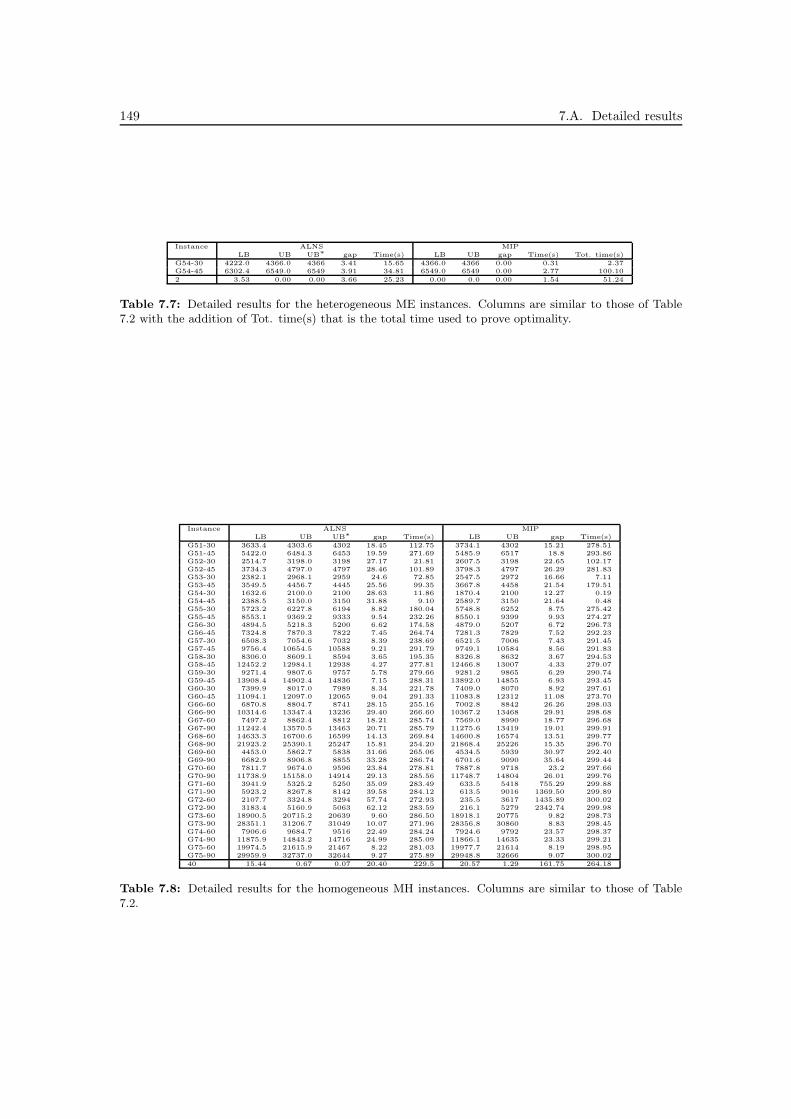
149 7.A. Detailed results
Instance ALNS MIPLB UB UB∗ gap Time(s) LB UB gap Time(s) Tot. time(s)
G54-30 4222.0 4366.0 4366 3.41 15.65 4366.0 4366 0.00 0.31 2.37G54-45 6302.4 6549.0 6549 3.91 34.81 6549.0 6549 0.00 2.77 100.10
2 3.53 0.00 0.00 3.66 25.23 0.00 0.0 0.00 1.54 51.24
Table 7.7: Detailed results for the heterogeneous ME instances. Columns are similar to those of Table7.2 with the addition of Tot. time(s) that is the total time used to prove optimality.
Instance ALNS MIPLB UB UB∗ gap Time(s) LB UB gap Time(s)
G51-30 3633.4 4303.6 4302 18.45 112.75 3734.1 4302 15.21 278.51G51-45 5422.0 6484.3 6453 19.59 271.69 5485.9 6517 18.8 293.86G52-30 2514.7 3198.0 3198 27.17 21.81 2607.5 3198 22.65 102.17G52-45 3734.3 4797.0 4797 28.46 101.89 3798.3 4797 26.29 281.83G53-30 2382.1 2968.1 2959 24.6 72.85 2547.5 2972 16.66 7.11G53-45 3549.5 4456.7 4445 25.56 99.35 3667.8 4458 21.54 179.51G54-30 1632.6 2100.0 2100 28.63 11.86 1870.4 2100 12.27 0.19G54-45 2388.5 3150.0 3150 31.88 9.10 2589.7 3150 21.64 0.48G55-30 5723.2 6227.8 6194 8.82 180.04 5748.8 6252 8.75 275.42G55-45 8553.1 9369.2 9333 9.54 232.26 8550.1 9399 9.93 274.27G56-30 4894.5 5218.3 5200 6.62 174.58 4879.0 5207 6.72 296.73G56-45 7324.8 7870.3 7822 7.45 264.74 7281.3 7829 7.52 292.23G57-30 6508.3 7054.6 7032 8.39 238.69 6521.5 7006 7.43 291.45G57-45 9756.4 10654.5 10588 9.21 291.79 9749.1 10584 8.56 291.83G58-30 8306.0 8609.1 8594 3.65 195.35 8326.8 8632 3.67 294.53G58-45 12452.2 12984.1 12938 4.27 277.81 12466.8 13007 4.33 279.07G59-30 9271.4 9807.6 9757 5.78 279.66 9281.2 9865 6.29 290.74G59-45 13908.4 14902.4 14836 7.15 288.31 13892.0 14855 6.93 293.45G60-30 7399.9 8017.0 7989 8.34 221.78 7409.0 8070 8.92 297.61G60-45 11094.1 12097.0 12065 9.04 291.33 11083.8 12312 11.08 273.70G66-60 6870.8 8804.7 8741 28.15 255.16 7002.8 8842 26.26 298.03G66-90 10314.6 13347.4 13236 29.40 266.60 10367.2 13468 29.91 298.68G67-60 7497.2 8862.4 8812 18.21 285.74 7569.0 8990 18.77 296.68G67-90 11242.4 13570.5 13463 20.71 285.79 11275.6 13419 19.01 299.91G68-60 14633.3 16700.6 16599 14.13 269.84 14600.8 16574 13.51 299.77G68-90 21923.2 25390.1 25247 15.81 254.20 21868.4 25226 15.35 296.70G69-60 4453.0 5862.7 5838 31.66 265.06 4534.5 5939 30.97 292.40G69-90 6682.9 8906.8 8855 33.28 286.74 6701.6 9090 35.64 299.44G70-60 7811.7 9674.0 9596 23.84 278.81 7887.8 9718 23.2 297.66G70-90 11738.9 15158.0 14914 29.13 285.56 11748.7 14804 26.01 299.76G71-60 3941.9 5325.2 5250 35.09 283.49 633.5 5418 755.29 299.88G71-90 5923.2 8267.8 8142 39.58 284.12 613.5 9016 1369.50 299.89G72-60 2107.7 3324.8 3294 57.74 272.93 235.5 3617 1435.89 300.02G72-90 3183.4 5160.9 5063 62.12 283.59 216.1 5279 2342.74 299.98G73-60 18900.5 20715.2 20639 9.60 286.50 18918.1 20775 9.82 298.73G73-90 28351.1 31206.7 31049 10.07 271.96 28356.8 30860 8.83 298.45G74-60 7906.6 9684.7 9516 22.49 284.24 7924.6 9792 23.57 298.37G74-90 11875.9 14843.2 14716 24.99 285.09 11866.1 14635 23.33 299.21G75-60 19974.5 21615.9 21467 8.22 281.03 19977.7 21614 8.19 298.95G75-90 29959.9 32737.0 32644 9.27 275.89 29948.8 32666 9.07 300.02
40 15.44 0.67 0.07 20.40 229.5 20.57 1.29 161.75 264.18
Table 7.8: Detailed results for the homogeneous MH instances. Columns are similar to those of Table7.2.

Bibliography 150
Instance ALNS MIPLB UB UB∗ gap Time(s) LB UB gap Time(s)
G51-30 7103.5 7368.0 7368 3.72 66.40 7346.7 7368 0.29 203.21G51-45 10635.0 11052.0 11052 3.92 158.16 10645.0 11052 3.82 276.38G52-30 2943.7 3546.0 3546 20.46 19.63 3255.3 3582 10.04 270.06G52-45 4393.5 5344.2 5319 21.64 81.09 4602.9 5368 16.62 274.87G53-30 3787.4 4350.9 4338 14.88 159.36 4008.3 4380 9.27 296.63G53-45 5678.9 6557.9 6507 15.48 239.63 5810.7 6574 13.14 298.56G55-30 9893.0 10640.3 10580 7.55 233.74 10101.7 10593 4.86 276.46G55-45 14783.0 16170.8 15935 9.39 272.15 14889.5 16070 7.93 290.26G56-30 10568.8 11277.5 11213 6.71 193.42 10821.9 11237 3.84 279.92G56-45 15797.3 16938.6 16858 7.22 261.75 15914.1 16929 6.38 289.14G57-30 8447.5 9217.1 9182 9.11 195.16 8460.1 9182 8.53 44.30G57-45 12628.0 13853.6 13795 9.71 198.80 12623.6 14238 12.79 2.24G58-30 14149.3 14681.4 14638 3.76 230.47 14243.2 14685 3.10 270.80G58-45 21211.7 22161.6 22055 4.48 283.90 21232.6 22081 4.00 275.67G59-30 19337.8 20281.7 20236 4.88 280.35 19423.8 19947 2.69 299.66G59-45 28997.8 30909.8 30637 6.59 276.55 29061.1 30563 5.17 296.37G60-30 16571.2 17044.6 16987 2.86 288.14 16604.5 17073 2.82 274.85G60-45 24849.9 25931.2 25791 4.35 280.39 24869.1 25638 3.09 294.97G66-60 10913.7 12671.5 12464 16.11 257.85 11039.8 12642 14.51 291.15G66-90 16355.9 19260.7 18901 17.76 286.09 16443.4 18985 15.46 296.29G67-60 13951.8 18038.9 17656 29.29 291.98 14300.4 17399 21.67 299.84G67-90 20797.0 27224.3 26982 30.90 280.03 20825.0 26537 27.43 299.90G68-60 32375.6 36315.6 36088 12.17 279.31 32292.0 35992 11.46 295.88G68-90 48475.4 54950.7 54481 13.36 278.92 48361.1 54223 12.12 295.97G69-60 6423.7 8302.3 8269 29.24 227.37 6664.7 8401 26.05 289.79G69-90 9654.3 12577.3 12459 30.28 273.90 9782.8 12748 30.31 297.31G70-60 24925.5 29187.2 28955 17.10 284.67 25239.1 29375 16.39 291.95G70-90 37389.5 45072.3 44772 20.55 287.02 37632.0 43981 16.87 295.89G71-60 5808.3 7769.1 7690 33.76 289.09 774.4 8061 940.90 294.17G71-90 8740.7 12075.9 11824 38.16 284.05 856.1 13082 1428.08 299.45G72-60 2484.1 3501.3 3454 40.95 278.58 330.4 3627 997.84 296.91G72-90 3667.3 5565.1 5427 51.75 286.58 291.1 5779 1885.34 299.84G73-60 38992.7 41590.9 41352 6.66 273.98 38985.0 41103 5.43 295.73G73-90 58468.4 63192.7 62987 8.08 258.80 58423.6 62408 6.82 298.88G74-60 9985.0 12115.1 11909 21.33 287.41 10023.9 12324 22.95 296.89G74-90 14995.2 18473.5 18241 23.20 283.09 15005.3 18142 20.90 291.21G75-60 41221.6 44762.1 43794 8.59 276.80 41308.6 43579 5.50 298.16G75-90 61823.9 67228.9 66664 8.74 265.99 61833.2 66533 7.60 300.11
38 12.12 1.16 0.28 16.18 243.44 17.83 1.25 148.21 274.73
Table 7.9: Detailed results for the heterogeneous MH instances. Columns are similar to those of Table7.2.
Bibliography
Achterberg, T., Berthold, T. Improving the feasibility pump. Discrete Optimization, 4(1):77–86,2007.
Belvaux, G., Wolsey, L. bc–prod: A specialized branch-and-cut system for lot-sizing. ManagementScience, 46(5):724–738, 2000.
Bertacco, L., Fischetti, M., Lodi, A. A feasibility pump heuristic for general mixed-integer prob-lems. Discrete Optimization, 4(1):63–76, 2007.
Burke, E., Kendall, G., Newall, J., Hart, E., Ross, P., Schulenburg, S. Hyper-heuristics: Anemerging direction in modern search technology. In Glover, F., Kochenberger, G., editors,Handbook of Meta-heuristics, chapter 16, pages 457–474. Kluwer, 2003.
Buschkuhl, L., Sahling, F., Helber, S., Tempelmeier, H. Dynamic capacitated lot-sizing problems:a classification and review of solution approaches. OR spectrum, 32(2):231–261, 2010.
Caserta, M., Rico, E. A cross entropy-Lagrangean hybrid algorithm for the multi-item capacitatedlot-sizing problem with setup times. Computers & Operations Research, 36(2):530–548, 2009.
Cordeau, J.-F., Laporte, G., Pasin, F., Ropke, S. Scheduling technicians and tasks in a telecom-munications company. Journal of Scheduling, 13:393–409, 2010.
Danna, E., Rothberg, E., Pape, C. L. Exploring relaxation induced neighborhoods to improve mipsolutions. Mathematical Programming, A(102):71–90, 2005.
Degraeve, Z., Jans, R. A new dantzig-wolfe reformulation and branch-and-price algorithm for thecapacitated lot-sizing problem with setup times. Operations Research, 55(5):909–920, 2007.
Denizel, M., Sural, H. On alternative mixed integer programming formulations and LP-basedheuristics for lot-sizing with setup times. Journal of the Operational Research Society, 57(4):389–399, 2006.

151 Bibliography
Fischetti, M., Lodi, A. Local branching. Mathematical Programming, 98:23–47, 2003.
Fischetti, M., Glover, F., Lodi, A. The feasibility pump. Mathematical Programming, 104(1):91–104, 2005.
Gopalakrishnan, M., Ding, K., Bourjolly, J., Mohan, S. A tabu-search heuristic for the capacitatedlot-sizing problem with set-up carryover. Management Science, 47(6):851–863, 2001.
Hindi, K., Fleszar, K., Charalambous, C. An effective heuristic for the clsp with set-up times.Journal of the Operational Research Society, 54:490 – 498, 2003.
Jans, R., Degraeve, Z. Meta-heuristics for dynamic lot-sizing: A review and comparison of solutionapproaches. European Journal of Operation Research, 177(3):1855–1875, 2007.
Maes, J., McClain, J., Van Wassenhove, L. Multilevel capacitated lotsizing complexity and LP-based heuristics. European Journal of Operational Research, 53(2):131–148, 1991.
Miller, A., Nemhauser, G., Savelsbergh, M. Solving multi-item capacitated lot-sizing problemswith setup times by branch-and-cut. Technical Report 39, Center for Operations Research andEconometrics, Universite Catholique de Louvain, Belgium, 2000.
Mladenovic, N., Hansen, P. Variable neighborhood search. Computers and Operations Research,24:1097–1100, 1997.
Muller, L. F. An adaptive large neighborhood search algorithm for the resource-constrained projectscheduling problem. In Proceedings of the VIII Metaheuristics International Conference (MIC)2009, Hamburg, Germany, 13-16 July 2009.
Pisinger, D., Røpke, S. A general heuristic for vehicle routing problems. Computers and OperationsResearch, 34(8):2403–2435, 2007.
Pisinger, D., Røpke, S. Large neighborhood search. In Gendreau, M., Potvin, J.-Y., editors,Handbook of Metaheuristics. Springer Verlag, 2nd edition, 2010.
Pochet, Y., Wolsey, L. Production Planning in Mixed Integer Programming. Springer, 2006.
Røpke, S., Pisinger, D. An adaptive large neighborhood search heuristic for the pickup and deliveryproblem with time windows. Transportation Science, 40(4):455–472, 2006.
Shaw, P. Using constraint programming and local search methods to solve vehicle routing prob-lems. CP-98 (Fourth International Conference on Principles and Practice of Constraint Pro-gramming), 1520:417–431, 1998.
Sural, H., Denizel, M., Wassenhove, L. V. Lagrangean based heuristics for lot-sizing with setuptimes. European Journal of Operational Research, 194:51–63, 2009.
Trigeiro, W., Thomas, L., McClain, J. Capacitated lot sizing with setup times. ManagementScience, 35(3):353–366, 1989.
Wolsey, L. Solving multi-item lot-sizing problems with an MIP solver using classification andreformulation. Management Science, 48(12):1587–1602, 2002.

Bibliography 152

Chapter 8
Conclusion
8.1 Summary, perspectives, and further research
In the following we give a summary of the work presented in this thesis, and discuss some per-spectives and suggestions for further research. The main topic has been scheduling problems, inparticular the Resource-Constrained Project Scheduling Problem (RCPSP), and to a lesser extendproduction planning problems.
The Resource-Constrained Project Scheduling Problem In Chapter 2 we developed anAdaptive Large Neighborhood Search (ALNS) heuristic for the single-mode RCPSP, and in Chap-ter 3 we extended this heuristic to the multi-mode RCPSP. Computational experiments on a largeset of benchmark instances from the PSPLIB showed that the single-mode algorithm was amongthe five best heuristics from the literature, and the multi-mode algorithm was among the threebest heuristics from the literature. For the multi-mode case, we found three new upper boundsfor instances of the J30 benchmark class.
The heuristic developed for the multi-mode RCPSP incorporated a new method, mode-diminu-tion, for removing modes during execution, and a simple technique, opportunistic mode-flipping,which can be applied whenever a schedule is generated, and which significantly improved theresults of the algorithm. These methods are generally applicable and it would be of interest toinvestigate whether these techniques could be beneficially incorporated into other algorithms forthe problem.
We proposed and experimented with three new lower bounds for the multi-mode RCPSP.One lower bound is based on a Lagrange relaxation and is an extension of the capacity bound,while the two others are based on testing all combinations of mode assignments for respectivelypairs and triples of activities. For the lower bound arguments examined, these new lower boundsproduced the best results, though at the cost of additional computational time. As most lowerbound arguments found in the literature target the single-mode RCPSP, it could be of interest tofurther examine multi-mode specific lower bounds.
For both algorithms the computational experiments showed that the adaptive component ofthe algorithm had a very small impact. It could be of interest to examine the reason for thismore closely, and to experiment with other types of methods for selecting neighborhoods, thanthe score based approach currently used. Such research would not only be of interest for thepresented algorithms, but also for the ALNS framework as a hole.
In connection with the ALNS algorithm developed for the multi-mode RCPSP the techniquesof precedence augmentation and mode-diminution was used to reduce the search space. Boththese techniques make use of lower bound arguments and it is somewhat surprising, that usingthe simple critical path lower bound, as opposed to a stronger lower bound, only has a very smallimpact on the results and a further investigation of the reason for this could be of interest. Forinstance, perhaps some structure of the problem could be identified which correlates with theeffectiveness of using the stronger lower bounds.
153

Chapter 8. Conclusion 154
The Multi-Mode RCPSP with Stochastic Nonrenewable Resource Consumption InChapter 5, we proposed and modeled a new variant of the multi-mode RCPSP where the non-renewable resource consumption of each mode is given by a Gaussian distribution, and the goalis to find a minimal makespan schedule which satisfies the nonrenewable resources with a certainprobability ǫ.
We developed a branch-and-cut algorithm where, in each node of the branch-and-bound tree,the branching decisions are propagated in order to remove variables from the problem, and thusimprove the lower bound used to prune the branch-and-bound tree. We experiment with cuttingon the conic quadratic resource constraints using the cuts presented in Chapter 4.
An adapted version of the ALNS algorithm presented in Chapter 3 was used to find initialupper bounds. These upper bounds were, for the instances where optimal solutions are known,on average less than one percent from the optimal solutions.
Experiments showed that propagating branching decisions was effective, and the branch-and-cut algorithm was able to outperform CPLEX 12.1. We finally examined the “cost of uncertainty”by investigating the relation between values of ǫ, the makespan, and the solution time. Theseexperiments showed that taking robustness into account only increases the makespan by about7% on average, while not increasing the computation time dramatically.
It could be interesting to merge the proposed model, with other stochastic variants of themulti-mode RCPSP, such as the variant with stochastic activity durations. In a heuristic setting,this should be quite easy, as only the evaluation of the nonrenewable resource constraints needs tobe changed to take into account the extra square-root term. In an exact setting, where a MixedInteger Programming (MIP) solver is used incorporating the stochastic nonrenewable resourceconstraints should also be quite easy, the main inconvenience being that the problem is now aquadratic integer program, rather than a linear one.
A further direction of research could be to investigate the formulation of other stochasticRCPSPs using chance constraints. For instance, modeling stochastic activity durations usingchance constraints could be very interesting, but could also prove a challenge, as the precedenceconstraints impose non-trivial dependencies between the starting time of the activities.
Second-order conic knapsack constraints In Chapter 4, we treated the subject of separatingand extending cover cuts for the second-order conic equivalent of the classic knapsack constraints,where the variables were additionally subject to generalized upper bound (GUB) constraints.
We showed how the the cover cuts can be extended by using the structure imposed by GUBconstraints, proposed a number of separation and extension algorithms, and compared these withCPLEX 12.1 on a set of generated test instances. These experiments showed that a relativelysimple separation and extension algorithm, which employs the structure imposed by the GUBconstraints, could speed up the solution time considerably.
As a theoretical contribution we showed that the problem of deciding if a cover can be extendedwith a variable is NP-hard, and established the relation between two bounds used in connectionwith the extension algorithms.
The work presented was mainly of a computational nature, and a possibility for further researchcould be to analyze the theoretical results from the classic knapsack constraints, and generalizethese results to the second-order cone case.
ROADEF/EURO 2010 In Chapter 6, we developed a Benders Decomposition approach tosolve a large scale energy management problem posed for the ROADEF/EURO 2010 challenge.As part of the approach we moddeled the problem as an MIP and experimented with differentadditional constraints for ensuring feasibility of subproblems. The problem size is quite large andwe presented a very effective preprocessing and aggregation scheme, which reduces the size of theproblem significantly. Because of the nature of some of the constraints, these could not be includedin the MIP and we presented an algorithm which takes a solution from the MIP and “repairs” itorder to make the solution satisfy the remaining constraints

155 8.2. General thoughts
On a set of smaller instances the approach was competitive, while on a set of larger instances itwas outperformed by local-search heuristics. This is mainly due to the size of the larger instancesin combination with the time allotted. On the instances used for rating the competitors, weplaced 14th out of 19 teams in the final of the competition. Being one of the few optimal methodsproposed, the algorithm was unable to compete with the heuristics given only 3600 seconds ofcomputing time. The sophisticated approach can, however, provide insights into the structure ofthe problem and information as to the quality of solutions through the lower bound informationwhich can be obtained at each iteration of the Benders algorithm.
Even though the competition is over, the group behind the challenge is still interested infurther research on the topic and they are maintaining results and problem instances on-line. Onedirection for further research could be to try to improve the proposed MIP model of the problem.More specifically to examine whether the non-linear constraints, currently not included in themodel, could be added (or approximated) without an explosion in the number of variables andconstraints needed. Another possibility would be to experiment with non-linear models.
We remind the reader that given a solution to the MIP model, a heuristic was applied to“repair” the solution in order to make it satisfy additional constraints not part of the model. Adirection for further research could be to improve this heuristic, by for instance leveraging thenetwork-flow structure of the problem.
From a theoretical perspective, a direction for research could be examining the complexity ofthe problem, and to investigate its structure more closely. For instance, the cost of a solution iscomposed of the cost of refueling and the cost of satisfying demand across a number of scenarios,and it would be of interest to analyse where the biggest cost contribution comes from. This wouldenable one to focus the algorithmic effort on the part of the problem having the most impact onthe cost.
Hybrid Adaptive Large Neighborhood Search In Chapter 7, we presented a hybrid heuris-tic solution approach based on the ALNS framework where a MIP solver was used in the repairphase. This results in a general hybrid ALNS algorithm where i) the “difficult” part of creatingrepair neighborhoods has been eliminated and ii) the strength of modern MIP solvers can beexploited.
The proposed hybrid algorithm was applied to a lot-sizing problem and the computationalresults indicate that the heuristic is very competitive. On a set of benchmark instances from theliterature combined with a new set of larger instances generated, the ALNS algorithm was able tooutperform the commercial MIP solver CPLEX 12.1.
Both the ALNS heuristic and the MIP solver outperformed the best heuristic found in theliterature, both with respect to the quality of the solution and the lower bounds produced. Thisindicates that it may be beneficial to use general MIP based repair neighborhoods in combinationwith problem specific destroy neighborhoods in ALNS.
Taking the best upper and lower bounds found by either the ALNS heuristic or the MIPsolver, we were able to improve upon 60 (out of 100) upper bounds and all lower bounds on a setof benchmark instances from the literature.
A suggestion for a future improvement is to apply the hybrid ALNS heuristic within thereoptimization process in the repair neighborhood. When solving larger problems the MIP solvermay become too slow to use in the repair neighborhoods, and it may be beneficial to apply ameta-heuristic approach to reoptimize the subproblem. This approach can be applied recursivelyuntil the subproblems are small enough for the MIP solver to be handled efficiently.
8.2 General thoughts
We now leave the topics covered directly by the chapters of the thesis in order to present somemore general thoughts.
Very little work seems to have been done on branch-and-price algorithms for the RCPSP, andinvestigating such algorithms could be interesting given the level of success of branch-and-price

Bibliography 156
algorithms within other fields of combinatorial optimization. One direction for research could bebased on the arc-flow formulation of the RCPSP proposed by Artigues et al. (2003). Restatingtheir model using path-flows instead of arc-flows results in a model with exponentially manycolumns, which could be well-suited for a branch-and-price approach. Another possibility couldbe based on the column-based formulation of Mingozzi et al. (1998) (see Section 1.3.1).
The best performing heuristics for the RCPSP seems to be population based heuristics and oneinteresting question is why population based approaches perform better than other approaches?Is it some property of the RCPSP or is it just because population based heuristics, are the petapproaches of researches within this area?
A promising technique seems to be to split the RCPSP into subproblems, apply a heuristic orexact solution method to the subproblems, and then recombine these solution into a solution tothe complete problem. An interesting direction of research, could be to examine different ways ofsplitting the RCPSP into smaller problems, and how to recombine these, both in a heuristic andexact context. Perhaps information derived from one splitting of the problem, could be used toinduce a new splitting.
For the current heuristic approaches that use splitting, typically the same algorithm is appliedto every subproblem, but perhaps one type of algorithm would be better to use in the early partsof the problem, while another type would be better in later parts. Perhaps other characteristicsof the subproblems could also be used to select the type of algorithm to use, such as the networkcomplexity, resource strength, or resource factor described in Section 1.3.3.
8.3 Final words
Scheduling and production planning is a fascinating field of research with both theoretical andpractical applications. The field is fascinating, not least because some of the problems, such asthe RCPSP, has been around for a long time, and even though the field has been very active, weare still only able to solve relatively small instances to optimality. It seems there are still newsolution methods to be discovered and insights to be gained, before we can consistently solve thekinds of scheduling and production planning problems considered in this thesis, and I would behappy if I through this work could be but a tiny stumble towards this goal.
Bibliography
Artigues, C., Michelon, P., Reusser, S. Insertion techniques for static and dynamic resource-constrained project scheduling. European Journal of Operational Research, 149(2):249 – 267,2003. Sequencing and Scheduling.
Mingozzi, A., Maniezzo, V., Ricciardelli, S., Bianco, L. An exact algorithm for the resource-constrained project scheduling problem based on a new mathematical formulation. ManagementScience, 44(5):714–729, 1998.