Embed Size (px)
Citation preview

Mean Variance Optimization
1/87
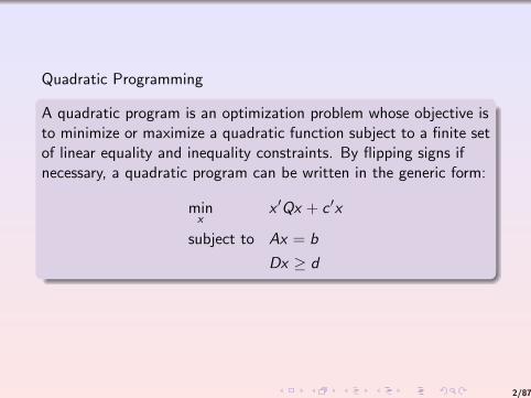
Quadratic Programming
A quadratic program is an optimization problem whose objective isto minimize or maximize a quadratic function subject to a finite setof linear equality and inequality constraints. By flipping signs ifnecessary, a quadratic program can be written in the generic form:
minx
x ′Qx + c ′x
subject to Ax = b
Dx ≥ d
2/87
Quadratic Programming
Quadratic programming models arise in a variety of practicalcontexts.
The seminal mean-variance model of Markowitz and most of itsvariants for portfolio selection are quadratic programs.
The popular ordinary least-squares and lasso estimation proceduresin linear regression are also quadratic programs.
Quadratic programs are also often solved as subproblems in thesolution of more general nonlinear optimization problems.
3/87

Quadratic Programming
A quadratic programming model is in standard form if it is writtenas follows:
minx
x ′Qx + c ′x
subject to Ax = b
x ≥ 0
4/87
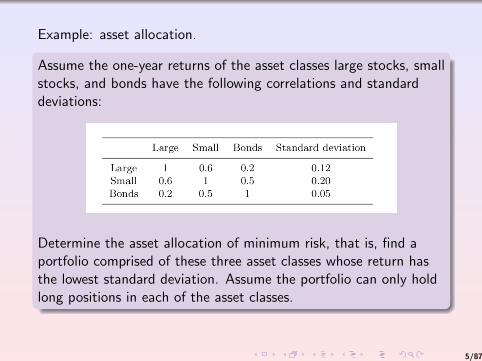
Example: asset allocation.
Assume the one-year returns of the asset classes large stocks, smallstocks, and bonds have the following correlations and standarddeviations:
Determine the asset allocation of minimum risk, that is, find aportfolio comprised of these three asset classes whose return hasthe lowest standard deviation. Assume the portfolio can only holdlong positions in each of the asset classes.
5/87
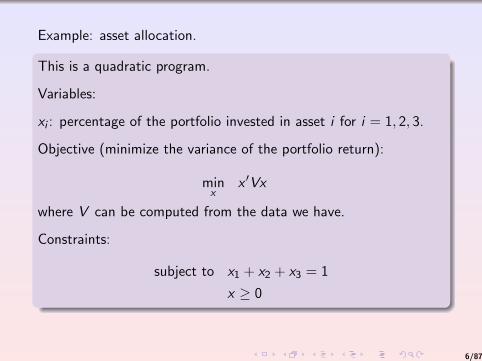
Example: asset allocation.
This is a quadratic program.
Variables:
xi : percentage of the portfolio invested in asset i for i = 1, 2, 3.
Objective (minimize the variance of the portfolio return):
minx
x ′Vx
where V can be computed from the data we have.
Constraints:
subject to x1 + x2 + x3 = 1
x ≥ 0
6/87

Quadratic Programming: No constraints
Suppose that we are dealing with:
minx
1
2x ′Qx
where Q is symmetric, positive definite.
Then x is an optimal solution if and only if:
Qx + c = 0.
7/87

Example: OLS revisited
Y = β′X + ε
Then, minimizing the squares:
(Xβ − y)′(Xβ − y) = β′X ′Xβ − 2y ′Xβ + y ′y
8/87
Example: OLS revisited
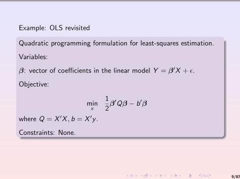
Quadratic programming formulation for least-squares estimation.
Variables:
β: vector of coefficients in the linear model Y = β′X + ε.
Objective:
minx
1
2β′Qβ − b′β
where Q = X ′X , b = X ′y .
Constraints: None.
9/87
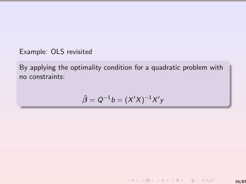
Example: OLS revisited
By applying the optimality condition for a quadratic problem withno constraints:
β = Q−1b = (X ′X )−1X ′y
10/87
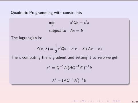
Quadratic Programming with constraints
minx
x ′Qx + c ′x
subject to Ax = b
The lagrangian is:
L(x , λ) =1
2x ′Qx + c ′x − λ′ (Ax − b)
Then, computing the x gradient and setting it to zero we get:
x∗ = Q−1A′(AQ−1A′)−1b
λ∗ = (AQ−1A′)−1b
11/87
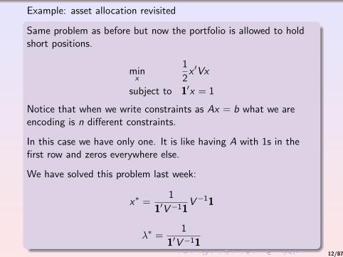
Example: asset allocation revisited
Same problem as before but now the portfolio is allowed to holdshort positions.
minx
1
2x ′Vx
subject to 1′x = 1
Notice that when we write constraints as Ax = b what we areencoding is n different constraints.
In this case we have only one. It is like having A with 1s in thefirst row and zeros everywhere else.
We have solved this problem last week:
x∗ =1
1′V−11V−11
λ∗ =1
1′V−1112/87
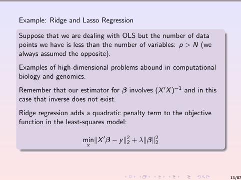
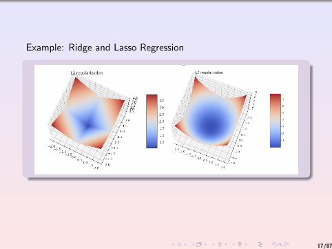
Example: Ridge and Lasso Regression
Suppose that we are dealing with OLS but the number of datapoints we have is less than the number of variables: p > N (wealways assumed the opposite).
Examples of high-dimensional problems abound in computationalbiology and genomics.
Remember that our estimator for β involves (X ′X )−1 and in thiscase that inverse does not exist.
Ridge regression adds a quadratic penalty term to the objectivefunction in the least-squares model:
minx‖X ′β − y‖22 + λ‖β‖22
13/87
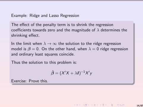
Example: Ridge and Lasso Regression
The effect of the penalty term is to shrink the regressioncoefficients towards zero and the magnitude of λ determines theshrinking effect.
In the limit when λ→∞ the solution to the ridge regressionmodel is β = 0. On the other hand, when λ = 0 ridge regressionand ordinary least squares coincide.
Thus the solution to this problem is:
β = (X ′X + λI )−1X ′y
Exercise: Prove this.
14/87
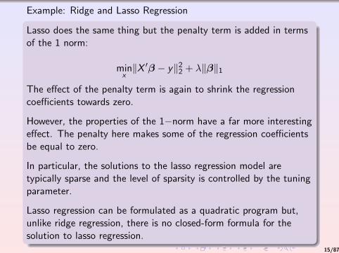
Example: Ridge and Lasso Regression
Lasso does the same thing but the penalty term is added in termsof the 1 norm:
minx‖X ′β − y‖22 + λ‖β‖1
The effect of the penalty term is again to shrink the regressioncoefficients towards zero.
However, the properties of the 1−norm have a far more interestingeffect. The penalty here makes some of the regression coefficientsbe equal to zero.
In particular, the solutions to the lasso regression model aretypically sparse and the level of sparsity is controlled by the tuningparameter.
Lasso regression can be formulated as a quadratic program but,unlike ridge regression, there is no closed-form formula for thesolution to lasso regression.
15/87
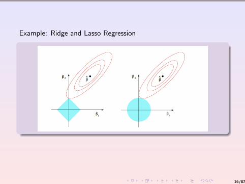
Example: Ridge and Lasso Regression
16/87
Example: Ridge and Lasso Regression
17/87

Portfolio Return
Suppose that we have n risky assets and let the vectors of assetprices at times t0 and t e:
v0 = (v1,0, . . . , vn,0)′, v = (v1, . . . , vn)′
We will form a portfolio with holdings h ∈ Rn. So the portfolioshave values:
W0 = h′v0,W = h′v
The returns of the portfolio and the individual assets are denotedby rP = W−W0
W0and ri =
vi−vi,0vi,0
.
Further, the percentage holdings are xi =hivi,0W0
.
18/87
Portfolio Return
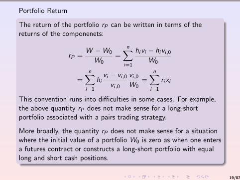
The return of the portfolio rP can be written in terms of thereturns of the componenets:
rP =W −W0
W0=
n∑i=1
hivi − hivi ,0W0
=n∑
i=1
hivi − vi ,0vi ,0
vi ,0W0
=n∑
i=1
rixi
This convention runs into difficulties in some cases. For example,the above quantity rP does not make sense for a long-shortportfolio associated with a pairs trading strategy.
More broadly, the quantity rP does not make sense for a situationwhere the initial value of a portfolio W0 is zero as when one entersa futures contract or constructs a long-short portfolio with equallong and short cash positions.
19/87
Portfolio Return
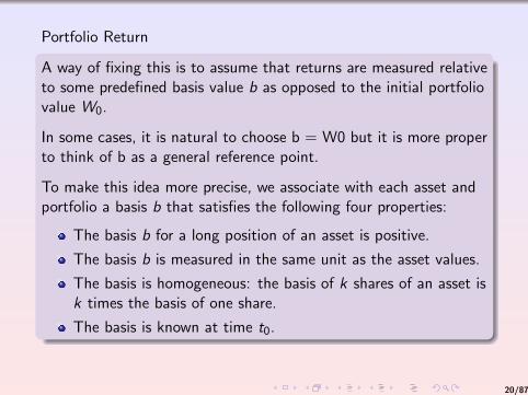
A way of fixing this is to assume that returns are measured relativeto some predefined basis value b as opposed to the initial portfoliovalue W0.
In some cases, it is natural to choose b = W0 but it is more properto think of b as a general reference point.
To make this idea more precise, we associate with each asset andportfolio a basis b that satisfies the following four properties:
The basis b for a long position of an asset is positive.
The basis b is measured in the same unit as the asset values.
The basis is homogeneous: the basis of k shares of an asset isk times the basis of one share.
The basis is known at time t0.
20/87

Portfolio Return
Equipped with this concept, we get a formal and unambiguousdefinition of asset and portfolio returns:
ri =vi − vi ,0
bi, rP =
W −W 0
bP
Likewise, we obtain a formal and unambiguous definition ofpercentage holdings:
xi =hibibP
21/87

Markowitz Mean-Variance
Markowitz’s key insight into the above one-period investmentproblem was to consider the expected value and standard deviationof the return as measures of performance and risk respectively.The portfolio selection problem can then be formally stated as aquadratic programming model.
To simplify our discussion of this model, we will proceed in threeincremental steps. First, we will look at the case when there areonly two assets; second, we will look at the case when there arethree risky assets; and finally, we will see the general case with anynumber of risky assets.
22/87
Markowitz Mean-Variance: two risky assets.
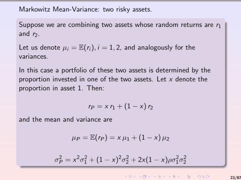
Suppose we are combining two assets whose random returns are r1and r2.
Let us denote µi = E(ri ), i = 1, 2, and analogously for thevariances.
In this case a portfolio of these two assets is determined by theproportion invested in one of the two assets. Let x denote theproportion in asset 1. Then:
rP = x r1 + (1− x) r2
and the mean and variance are
µP = E(rP) = x µ1 + (1− x)µ2
σ2P = x2σ21 + (1− x)2σ22 + 2x(1− x)ρσ21σ22
23/87
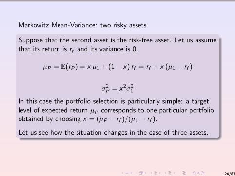
Markowitz Mean-Variance: two risky assets.
Suppose that the second asset is the risk-free asset. Let us assumethat its return is rf and its variance is 0.
µP = E(rP) = x µ1 + (1− x) rf = rf + x (µ1 − rf )
σ2P = x2σ21
In this case the portfolio selection is particularly simple: a targetlevel of expected return µP corresponds to one particular portfolioobtained by choosing x = (µP − rf )/(µ1 − rf ).
Let us see how the situation changes in the case of three assets.
24/87
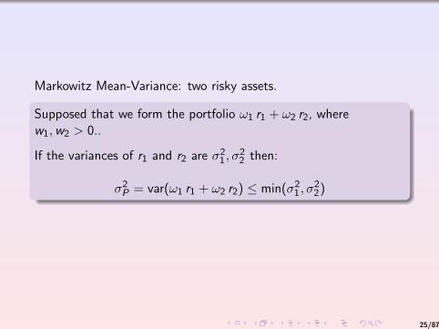
Markowitz Mean-Variance: two risky assets.
Supposed that we form the portfolio ω1 r1 + ω2 r2, wherew1,w2 > 0..
If the variances of r1 and r2 are σ21, σ22 then:
σ2P = var(ω1 r1 + ω2 r2) ≤ min(σ21, σ22)
25/87
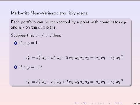
Markowitz Mean-Variance: two risky assets.
Each portfolio can be represented by a point with coordinates σVand µV on the σ, µ plane.
Suppose that σ1 6= σ2, then:
1 If ρ1,2 = 1:
σ2V = σ21 w1 + σ22 w2 − 2w1 w2 σ1 σ2 = |σ1 w1 − σ2 w2|2
2 If ρ1,2 = −1:
σ2V = σ21 w1 + σ22 w2 + 2w1 w2 σ1 σ2 = |σ1 w1 + σ2 w2|2
26/87
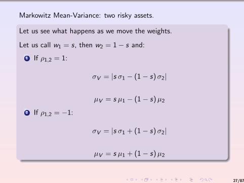
Markowitz Mean-Variance: two risky assets.
Let us see what happens as we move the weights.
Let us call w1 = s, then w2 = 1− s and:
1 If ρ1,2 = 1:
σV = |s σ1 − (1− s)σ2|
µV = s µ1 − (1− s)µ2
2 If ρ1,2 = −1:
σV = |s σ1 + (1− s)σ2|
µV = s µ1 + (1− s)µ2
27/87
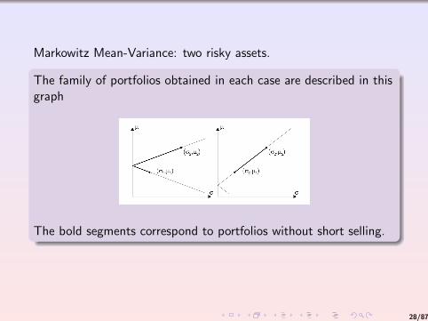
Markowitz Mean-Variance: two risky assets.
The family of portfolios obtained in each case are described in thisgraph
The bold segments correspond to portfolios without short selling.
28/87
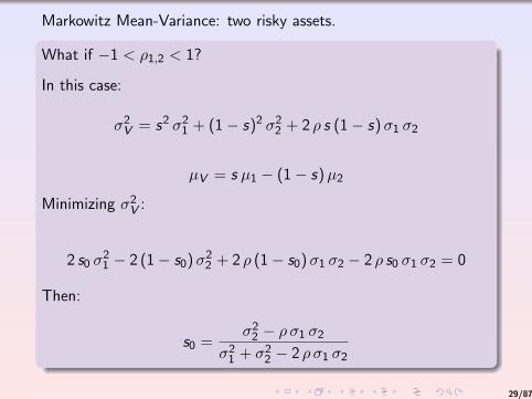
Markowitz Mean-Variance: two risky assets.
What if −1 < ρ1,2 < 1?
In this case:
σ2V = s2 σ21 + (1− s)2 σ22 + 2 ρ s (1− s)σ1 σ2
µV = s µ1 − (1− s)µ2
Minimizing σ2V :
2 s0 σ21 − 2 (1− s0)σ22 + 2 ρ (1− s0)σ1 σ2 − 2 ρ s0 σ1 σ2 = 0
Then:
s0 =σ22 − ρ σ1 σ2
σ21 + σ22 − 2 ρ σ1 σ2
29/87
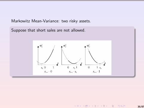
Markowitz Mean-Variance: two risky assets.
Suppose that short sales are not allowed.
30/87
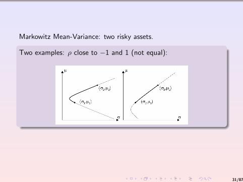
Markowitz Mean-Variance: two risky assets.
Two examples: ρ close to −1 and 1 (not equal):
31/87
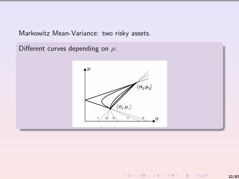
Markowitz Mean-Variance: two risky assets.
Different curves depending on ρ:
32/87
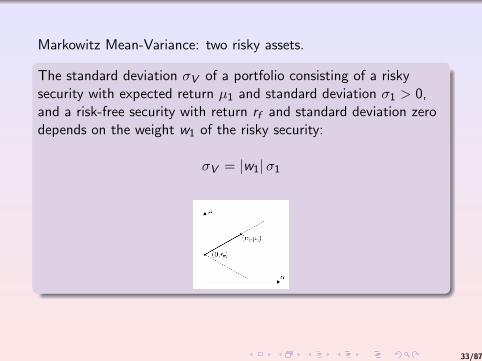
Markowitz Mean-Variance: two risky assets.
The standard deviation σV of a portfolio consisting of a riskysecurity with expected return µ1 and standard deviation σ1 > 0,and a risk-free security with return rf and standard deviation zerodepends on the weight w1 of the risky security:
σV = |w1|σ1
33/87
Markowitz Mean-Variance: three risky assets.
µP = x1 µ1 + x2 µ2 + x3 µ3
σ2P = x21σ21 + x22σ
22 + x23σ
23 + 2(σ12σ
21σ
22 + σ13σ
21σ
23 + σ23σ
22σ
23)
Now there are multiple portfolios that can achieve a targetexpected level of return.
34/87
Markowitz Mean-Variance: three risky assets.
A portfolio is efficient if it has minimum risk for a given targetreturn, or equivalently, if it has the maximum expected return for agiven target risk. This naturally leads to the following quadraticprogramming formulation.
The efficient frontier is the set of efficient portfolios. The efficientfrontier is often ”visualized” by plotting the expected returnagainst the standard deviation of the efficient portfolios.
35/87
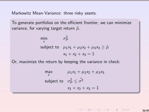
Markowitz Mean-Variance: three risky assets.
To generate portfolios on the efficient frontier, we can minimizevariance, for varying target return µ.
minx
σ2P
subject to µ1x1 + µ2x2 + µ3x3 ≥ µx1 + x2 + x3 = 1
Or, maximize the return by keeping the variance in check:
maxx
µ1x1 + µ2x2 + µ3x3
subject to σ2P ≤ σ2
x1 + x2 + x3 = 1
36/87
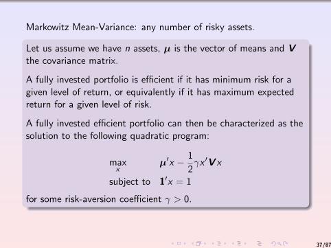
Markowitz Mean-Variance: any number of risky assets.
Let us assume we have n assets, µ is the vector of means and Vthe covariance matrix.
A fully invested portfolio is efficient if it has minimum risk for agiven level of return, or equivalently if it has maximum expectedreturn for a given level of risk.
A fully invested efficient portfolio can then be characterized as thesolution to the following quadratic program:
maxx
µ′x − 1
2γx ′V x
subject to 1′x = 1
for some risk-aversion coefficient γ > 0.
37/87
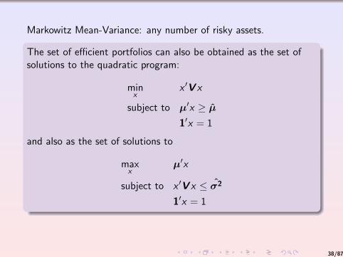
Markowitz Mean-Variance: any number of risky assets.
The set of efficient portfolios can also be obtained as the set ofsolutions to the quadratic program:
minx
x ′V x
subject to µ′x ≥ µ
1′x = 1
and also as the set of solutions to
maxx
µ′x
subject to x ′V x ≤ σ2
1′x = 1
38/87
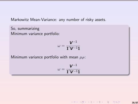
Markowitz Mean-Variance: any number of risky assets.
So, summarizingMinimum variance portfolio:
ω =V−1
1′V−11
Minimum variance portfolio with mean µP :
ω =V−1
1′V−11
39/87

Asset Allocation and Security Selection
There are two distinct levels of portfolio analysis that are amenableto mean-variance models.
The conventional top-down investment approach to portfolioconstruction consists of two main steps, namely asset allocationand security selection.
40/87
Asset Allocation and Security Selection
On the one hand, the asset allocation decision is concerned withportfolio choices among broad asset classes.
At the coarsest level, these asset classes could be stocks, bonds,and cash. At a more refined level, some of these broad assetclasses could be subdivided. For instance, stocks can be dividedaccording to geography or market capitalization. The assetallocation decision involves only a small number of assets, typicallyranging from a handful to a dozen or so. It generally involvessimple constraints such as budget constraints and upper and lowerbounds on individual positions.
41/87
Asset Allocation and Security Selection
On the other hand, the security selection decision is concernedwith the specific securities within each particular asset class. Forinstance, if the relevant asset class is equities in the S&P 500market index, then the security selection problem is concerned withthe specific portfolio holdings at the individual stock level.
The security selection problem typically involves a large number ofsecurities, ranging from a few hundred to potentially thousands. Italso involves a myriad of constraints and is often formulatedrelative to a predefined benchmark.
42/87
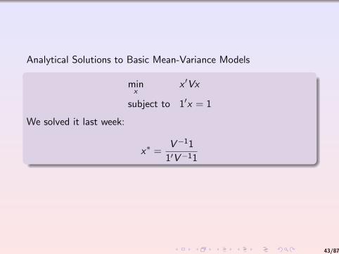
Analytical Solutions to Basic Mean-Variance Models
minx
x ′Vx
subject to 1′x = 1
We solved it last week:
x∗ =V−11
1′V−11
43/87
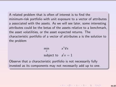
A related problem that is often of interest is to find theminimum-risk portfolio with unit exposure to a vector of attributesa associated with the assets. As we will see later, some interestingattributes could be the betas of the assets relative to a benchmark,the asset volatilities, or the asset expected returns. Thecharacteristic portfolio of a vector of attributes a is the solution tothe problem
minx
x ′Vx
subject to a′x = 1
Observe that a characteristic portfolio is not necessarily fullyinvested as its components may not necessarily add up to one.
44/87
Two-Fund Separation Theorem
Consider the basic mean-variance model
maxx
µ′x − 1
2γx ′V x
subject to 1′x = 1
for some risk-aversion coefficient γ > 0.
We next derive an interesting result often called the two-fundseparation theorem.
The theorem states that every fully invested efficient portfolio is acombination of two particular efficient portfolios.
45/87

Two-Fund Separation Theorem
The solution to that problem is:
x = λ1
1′VµV−1µ + (1− λ)cV−11
with:
λ =1′Vµ
γ
46/87
Two-Fund Separation Theorem
Two-fund theorem: Within the model we are considering (for someγ > 0), there exist two efficient portfolios, namely
1
1′VµV−1µ and
1
1′VµV−11
such that every efficient portfolio, that is, every solution is acombination of these two portfolios.
47/87
One-Fund Separation Theorem
If there is a risk-free asset, then every efficient portfolio is acombination of the risk-free asset and a particular fund.
Notation: the vector of n risky assets will be denoted by x .
maxx ,xn+1
µ′x + rf xn+1 −1
2γx ′Vx
subject to 1′x + xn+1 = 1
Replacing: xn+1 = 1− 1′x , we get:
maxx
(µ− rf 1)′x − 1
2γx ′Vx
48/87
One-Fund Separation Theorem: one-fund theorem.
One-fund theorem: suppose the investment universe includes nrisky assets and a risk-free asset. Then there exists a fully investedefficient portfolio (fund) namely
1
1′V−1(µ− rf 1)V−1(µ− rf 1)
such that every efficient portfolio (any portfolio solving theoptimization problem including the risk-free asset and for someγ > 0) is a combination of this portfolio and the risk-free asset.
49/87
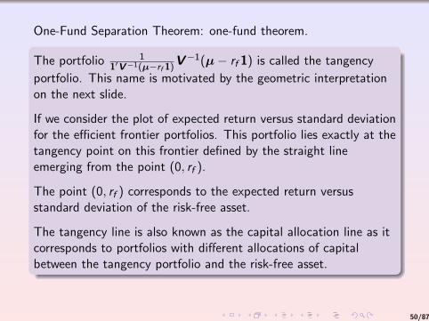
One-Fund Separation Theorem: one-fund theorem.
The portfolio 11′V−1(µ−rf 1)
V−1(µ− rf 1) is called the tangency
portfolio. This name is motivated by the geometric interpretationon the next slide.
If we consider the plot of expected return versus standard deviationfor the efficient frontier portfolios. This portfolio lies exactly at thetangency point on this frontier defined by the straight lineemerging from the point (0, rf ).
The point (0, rf ) corresponds to the expected return versusstandard deviation of the risk-free asset.
The tangency line is also known as the capital allocation line as itcorresponds to portfolios with different allocations of capitalbetween the tangency portfolio and the risk-free asset.
50/87

One-Fund Separation Theorem: one-fund theorem.
51/87
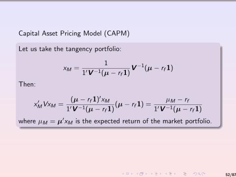
Capital Asset Pricing Model (CAPM)
Let us take the tangency portfolio:
xM =1
1′V−1(µ− rf 1)V−1(µ− rf 1)
Then:
x ′MVxM =(µ− rf 1)′xM
1′V−1(µ− rf 1)(µ− rf 1) =
µM − rf1′V−1(µ− rf 1)
where µM = µ′xM is the expected return of the market portfolio.
52/87
Capital Asset Pricing Model (CAPM)
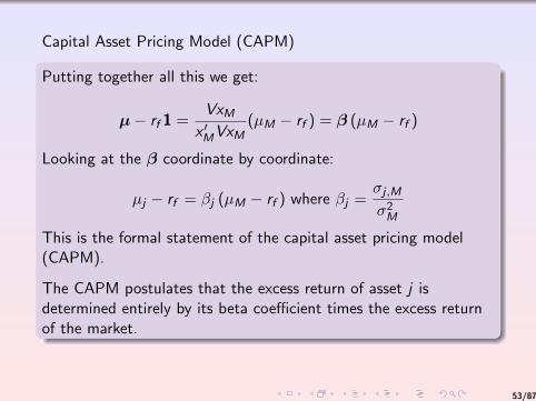
Putting together all this we get:
µ− rf 1 =VxM
x ′MVxM(µM − rf ) = β (µM − rf )
Looking at the β coordinate by coordinate:
µj − rf = βj (µM − rf ) where βj =σj ,Mσ2M
This is the formal statement of the capital asset pricing model(CAPM).
The CAPM postulates that the excess return of asset j isdetermined entirely by its beta coefficient times the excess returnof the market.
53/87

More General Mean-Variance Models
The basic mean-variance model discussed in the previous sectionprovides the foundation of modern portfolio theory.
However, when mean-variance models are used as a tool inportfolio construction, it is common to use modifications of thebasic model by including additional constraints and possiblyadditional terms in the objective.
54/87
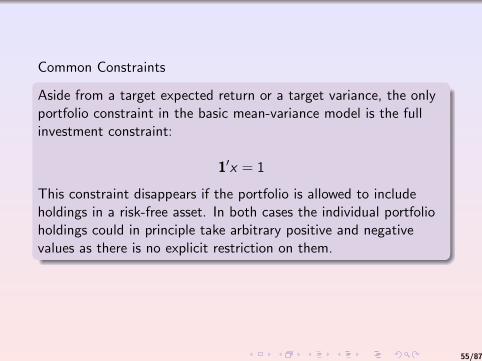
Common Constraints
Aside from a target expected return or a target variance, the onlyportfolio constraint in the basic mean-variance model is the fullinvestment constraint:
1′x = 1
This constraint disappears if the portfolio is allowed to includeholdings in a risk-free asset. In both cases the individual portfolioholdings could in principle take arbitrary positive and negativevalues as there is no explicit restriction on them.
55/87
Common Constraints
This motivates the following types of constraints that are oftenincluded in a mean-variance model:
Budget constraints, such as fully invested portfolios.
Upper and/or lower bounds on the size of individual positions.
Upper and/or lower bounds on exposure to industries orsectors.
Leverage constraints such as long-only, or 130/30 constraints.
Turnover constraints.
56/87
Common Constraints
So, we replace the constraint: 1′x = 1 y:
maxx
µ′x − 1
2γx ′V x
subject to Ax = bDx = d
for some risk-aversion coefficient γ > 0.
57/87

Common Constraints
As before, the set of efficient portfolios can also be obtained as theset of solutions to the quadratic program:
minx
x ′V x
subject to µ′x ≥ µ
Ax = bDx = d
and also as the set of solutions to
maxx
µ′x
subject to x ′V x ≤ σ2
Ax = bDx = d
58/87
Common Constraints
These models are still convex quadratic optimization models.
Unlike the basic mean-variance model, they generally do not havean analytical closed-form solution due to the additional inequalityconstraints.
However, they can be solved numerically very efficiently viaoptimization solvers.
59/87
Common Constraints: leverage constraints
Long-only constraint : x ≥ 0.
A relaxed version of this constraint, popular in certain contexts, isnot to rule out leverage altogether but to limit it.
For instance, a 130/30 leverage constraint means that the totalvalue of the holdings in short positions must be at most 30% ofthe portfolio value.
In general, suppose that we want the value of the total shortpositions to be at most L. This means that we want to enforce thefollowing restriction:
n∑j=1
min(xj , 0) ≥ −L
Solving that problem is not easy (not a quadratic program) butthis can be fixed by introducing an auxiliary variable y .
60/87
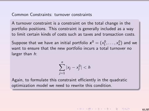
Common Constraints: turnover constraints
A turnover constraint is a constraint on the total change in theportfolio positions. This constraint is generally included as a wayto limit certain kinds of costs such as taxes and transaction costs.
Suppose that we have an initial portfolio x0 = (x01 , . . . , x0n ) and we
want to ensure that the new portfolio incurs a total turnover nolarger than h:
n∑j=1
|xj − x0j | < h
Again, to formulate this constraint efficiently in the quadraticoptimization model we need to rewrite this condition.
61/87
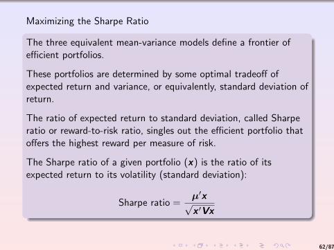
Maximizing the Sharpe Ratio
The three equivalent mean-variance models define a frontier ofefficient portfolios.
These portfolios are determined by some optimal tradeoff ofexpected return and variance, or equivalently, standard deviation ofreturn.
The ratio of expected return to standard deviation, called Sharperatio or reward-to-risk ratio, singles out the efficient portfolio thatoffers the highest reward per measure of risk.
The Sharpe ratio of a given portfolio (x) is the ratio of itsexpected return to its volatility (standard deviation):
Sharpe ratio =µ′x√x ′Vx
62/87
Maximizing the Sharpe Ratio
Sometimes µ may not necessarily stand for the vector of expectedabsolute returns but instead for the vector of expected relativereturns.
In particular, if there is a risk-free asset, in the above definition ofthe Sharpe ratio it is usual to assume that µ stands for the vectorof expected excess returns.The excess return of an asset is simply the difference of its returnand the risk-free return.
As an alternative or a complement to the equivalent mean-variancemodels consider the problem of finding the efficient portfolio withmaximum Sharpe ratio.
63/87
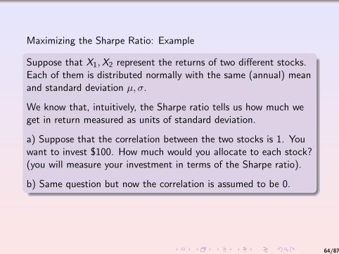
Maximizing the Sharpe Ratio: Example
Suppose that X1,X2 represent the returns of two different stocks.Each of them is distributed normally with the same (annual) meanand standard deviation µ, σ.
We know that, intuitively, the Sharpe ratio tells us how much weget in return measured as units of standard deviation.
a) Suppose that the correlation between the two stocks is 1. Youwant to invest $100. How much would you allocate to each stock?(you will measure your investment in terms of the Sharpe ratio).
b) Same question but now the correlation is assumed to be 0.
64/87
Maximizing the Sharpe Ratio
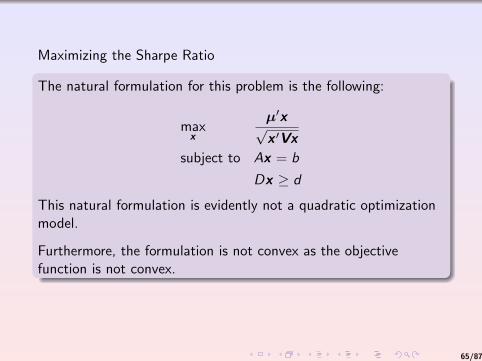
The natural formulation for this problem is the following:
maxx
µ′x√x ′Vx
subject to Ax = b
Dx ≥ d
This natural formulation is evidently not a quadratic optimizationmodel.
Furthermore, the formulation is not convex as the objectivefunction is not convex.
65/87
Maximizing the Sharpe Ratio
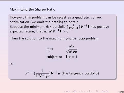
However, this problem can be recast as a quadratic convexoptimization (we omit the details) to obtain:.Suppose the minimum-risk portfolio ( 1
1′V−11)V−11 has positive
expected return; that is, µ′V−11 > 0.
Then the solution to the maximum Sharpe ratio problem
maxx
µ′x√x ′Vx
subject to 1′x = 1
is:
x∗ = (1
1′V−1µ)V−1µ (the tangency portfolio)
66/87

Portfolio Management Relative to a Benchmark
In an investment portfolio, the security selection problem isconcerned with determining the holdings of specific securitieswithin a given asset class.
It is customary to manage and evaluate the portfolio of securitiesrelative to some predefined benchmark portfolio that represents aparticular asset class.
The benchmark portfolio provides a reference point.
It serves the role of the market portfolio if the investment universeis restricted to the particular asset class that the benchmarkrepresents.
The management of a portfolio of securities relative to abenchmark could be passive or active.
The goal of the former is to replicate the benchmark whereas thegoal of the latter is to beat the benchmark.
67/87
Systematic (Beta) and Individual (Alpha) Returns.
Both passive and active management rely on a fundamentaldecomposition of individual securities return into systematic andindividual (or residual) components.
The former is the component of return that can be explained bythe security exposure to the benchmark.
The latter is the component of return that is idiosyncratic to theindividual security.
To make the above decomposition more precise, assume theinvestment universe determined by a particular asset class includesn individual securities.
68/87
Systematic (Beta) and Individual (Alpha) Returns.
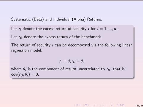
Let ri denote the excess return of security i for i = 1, ..., n.
Let rB denote the excess return of the benchmark.
The return of security i can be decomposed via the following linearregression model:
ri = βi rB + θi
where θi is the component of return uncorrelated to rB ; that is,cov(rB , θi ) = 0.
69/87
Systematic (Beta) and Individual (Alpha) Returns.
The coefficient βi is the beta of security i relative to thebenchmark B and is given by βi = cov(ri , rB)var(rB).
The term βi rB is the systematic component of return of security i .
The term θi is the residual component of return of security i .
The alpha of security i is the expected value of the residual returnθi :
αi = E(θi )
70/87
Systematic (Beta) and Individual (Alpha) Returns.
Consider a portfolio of securities with percentage holdingsx = (x1, . . . , xn)′.
The portfolio return is given by rP = r ′x , then:
rP = βP rB + θP
where βP = β′x , θP = θ′x , αP = α′x .
71/87
Estimation of Inputs to Mean-Variance Models
The estimation of input parameters, namely the covariance matrixof returns V and the vector of total expected returns µ is one ofthe most critical and challenging steps in the use of mean-variancemodels.
The naive way to estimate those is:
µ =1
T
T∑t=1
r(T ), V =1
T
T∑t=1
(r(T )− µ)(r(T )− µ)′
72/87
Estimation of Inputs to Mean-Variance Models: shortcomings ofthis approach
The sample mean and sample covariance do not incorporateother data that could contain useful forecasting information.
A lot of parameters to estimate.
The sample mean and sample covariance inevitably contain afair amount of estimation errors (which are magnified by themean-variance optimizer).
73/87
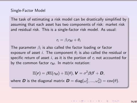
Single-Factor Model
The task of estimating a risk model can be drastically simplified byassuming that each asset has two components of risk: market riskand residual risk. This is a single-factor risk model. As usual:
ri = βi rM + θi
The parameter βi is also called the factor loading or factorexposure of asset i . The component θi is also called the residual orspecific return of asset i , as it is the portion of ri not accounted forby the common factor rM . In matrix notation:
E(r) = βE(rM) + E(θ),V = σ2ββ′ + D,
where D is the diagonal matrix D = diag(ω21, ..., ω
2n) = cov(θ).
74/87
Single-Factor Model
Under the single-factor model, the estimation of the covariancematrix only requires the estimation of β, σ2M , and D.
That is a total of n + 1 + n = 2n + 1 parameters in contrast to the12n(n + 1) parameters for a non-structured covariance matrix.
The particular structure of the covariance matrix for a single-factorrisk model also enables the derivation of some interestingproperties of minimum-risk portfolios.
75/87
Constant Correlation Models
A second way of imposing structure on the asset returns is toassume that the correlation between any two different assets in theinvestment universe is the same.
Under this assumption, the estimation of the covariance matrixonly requires an estimate of each individual asset volatility σi andthe average correlation ρ between different pairs of assets.
This yields a estimate of the covariance matrix given by
cov(ri , rj) = ρσiσj , i 6= j .
In this model the estimation of the covariance matrix only requiresestimates of σ and ρ. That is a total of n + 1 parameters.
Under the reasonable assumption that ρ > 0, the constantcorrelation model can be seen as a single-factor model withpredetermined factor loadings.
76/87

Multiple-Factor Models
Multiple-factor models are a generalization of the single-factormodel discussed above.
These models are based on the assumption that the return of eachasset can be explained by a small collection of common factors inaddition to some other specific return.
Aside from simplifying the estimation task, multiple-factor modelsprovide a useful breakdown of risk, incorporate some economiclogic, and are fairly flexible.
77/87
Multiple-Factor Models
A multi-factor model assumes that excess returns are as follows:
ri
K∑k=1
Bik fk + ui
ri : excess return of asset i .
Bik : exposure of asset i to factor k .
fk : rate of return of factor k .
ui : specific (or residual) return of asset i .
78/87
Sensitivity of Mean-Variance Models to Input Estimation
One of the most salient drawbacks of mean-variance optimizationis its high sensitivity to the estimation of input parameters.
The sensitivity is due to the very nature of the optimizationprocess: if there are assets whose returns appear to be superior,the portfolios generated by an optimization procedure will try totake advantage of these apparently superior assets byoverweighting the holdings on those positions.
Unfortunately in a practical setting there is inevitable noise in theestimation of inputs to a mean-variance model.
Small perturbations in the values of the inputs may lead to largeswings in the composition of the portfolio.
79/87
Sensitivity of Mean-Variance Models to Input Estimation
This unfortunate phenomenon is basically due to the fact that theoptimizer is overly responsive given the quality of the inputs typicalin portfolio construction.
A related phenomenon is the fact that the composition ofportfolios is often non-intuitive.
Theoretical and empirical evidence indicates that the estimate ofexpected returns is more critical than the estimate of thecovariance matrix.
The input sensitivity of mean-variance models is a central issue inportfolio management and has been a subject of intense study.
80/87
Sensitivity of Mean-Variance Models to Input Estimation
There is a tremendous upside potential in finding appropriate waysof harnessing the power of portfolio optimization without gettingcaught on this major shortcoming.
The techniques that aim at mitigating this probleman be classifiedin two main categories. The first category of techniques tries toimprove the quality of the inputs to the portfolio optimizationproblem. The second category of techniques aims to tweak theoptimization procedure.
One of the most widely used techniques in the first category is theBlack-Litterman model introduced by Fisher Black and BobLitterman at Goldman Sachs Asset Management.
81/87

Black-Litterman Model
The basic idea of the Black-Litterman model is to tilt the marketequilibrium returns to incorporate an investor’s views.
In principle a classical mean-variance model requires estimates ofexpected returns for all assets in the investment universeconsidered.
This is typically an enormous task. Investment managers areunlikely to have detailed knowledge of all securities at theirdisposal.
Typically, they have a specific area of expertise. Furthermore, somemodern trading strategies are associated not with absolute butwith relative rankings of securities.For instance, a pairs trading strategy corresponds to a forecastthat one stock will outperform another one.The key insight of Black and Litterman was that there is a suitableway of combining the investor’s views with the market equilibrium.
82/87
Black-Litterman Model: Basic Assumptions
The Black-Litterman model is an equilibrium-based model,meaning that the expected returns of the assets should beconsistent with the market equilibrium unless the investor has somespecific views.
In other words, an investor without any views on the market shouldhold the market. We shall let π denote the equilibrium returnvector, and V the covariance matrix of the asset returns.
The true expected return vector µ is unknown. As a starting point,we assume that the equilibrium return vector serves as a reasonableprior estimate of the true return vector in the sense that
µ ∼ N(π,Q)
That is, µ is a multi-normal random vector with expected value πand covariance matrix Q. The matrix Q represents the confidenceon the equilibrium returns as an estimate of expected returns.
83/87
Black-Litterman Model
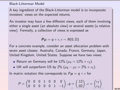
A key ingredient of the Black-Litterman model is to incorporateinvestors’ views on the expected returns.
An investor may have a few different views, each of them involvingeither a single asset (an absolute view) or several assets (a relativeview). Formally, a collection of views is expressed as
Pµ = q + ε, ε ∼ N(0,Ω)
For a concrete example, consider an asset allocation problem withseven asset classes: Australia, Canada, France, Germany, Japan,United Kingdom, United States. Suppose we have two views:
Return on Germany will be 12% (µ4 = 12% + ε1).
UK will outperform US by 2% (µ6 − µ7 = 2% + ε1).
In matrix notation this corresponds to Pµ = q + ε for
P =
(0 0 0 1 0 0 00 0 0 0 0 1 −1
), q =
(.12.02
), ε =
(ε1ε2
)????????????
84/87

Black-Litterman Model: Merging Investors’ Views and MarketEquilibrium
The key insight of the Black-Litterman model is a proper way tocombine the investor?s views with the prior market equilibrium.
So, we have µ ∼ N(π,Q) as a prior and our views are encoded asPµ = q + ε, where ε ∼ N(0,Ω).
We can write this as a system:
y = Mµ+ ε, ε ∼ N(0,Σ)
y =
(πq
),M =
(IP
),Σ =
(Q 00 Ω
)
85/87
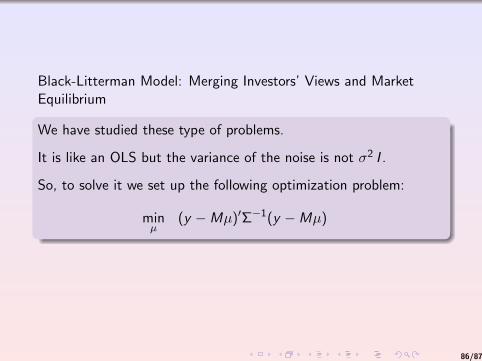
Black-Litterman Model: Merging Investors’ Views and MarketEquilibrium
We have studied these type of problems.
It is like an OLS but the variance of the noise is not σ2 I .
So, to solve it we set up the following optimization problem:
minµ
(y −Mµ)′Σ−1(y −Mµ)
86/87

Black-Litterman Model
Optimality says:
2M ′Σ−1Mµ− 2M ′Σ−1y = 0
Then:
µ = π + QP ′(PQP ′ + Ω)−1(q − Pπ).
87/87