International Journal of Bioinformatics and Biomedical Engineering

Vol. 1, No. 2, 2015, pp. 53-63

http://www.aiscience.org/journal/ijbbe

* Corresponding author E-mail address: mkowolax@yahoo.com, kowolabi@uwc.ac.za, kmowolabi@futa.edu.ng

Robust Numerical Solution of the Time-Dependent Problems with Blow-Up

Kolade M. Owolabi1, 2, *

1Department of Mathematical Sciences, Federal University of Technology, Ondo-State, Nigeria 2Department of Mathematics and Applied Mathematics, University of the Western Cape, Bellville, Republic of South Africa

Abstract

Numerical solutions of nonlinear time-dependent partial differential equations with blow-up are considered in this paper. Such systems of PDEs are categorized into linear and nonlinear parts to allow the use of two classic mathematical ideas in space and time. The main focus in this paper is to discretized in space with higher order finite difference approximation and integrate the resulting nonlinear ordinary differential equations with an adaptive fourth-order exponential time differencing Runge-Kutta (ETDRK4) scheme. Stability analysis of the scheme is also examined. This paper is primarily concerned with the use of the ETDRK4 method to simulate some of the blow-up phenomena in nonlinear parabolic equations that are largely encountered in a number of physical situations, like chemical reaction-diffusion, electrical heating, fluid flow and population growth. It is expected that the time at which blow-up occurs will reflect in the numerical results.

Keywords

Blow-Up Problems, Exponential Time Differencing Methods, Nonlinear, Time-Dependent Pdes, Stability

Received: June 10, 2015 / Accepted: June 26, 2015 / Published online: July 13, 2015

@ 2015 The Authors. Published by American Institute of Science. This Open Access article is under the CC BY-NC license.

http://creativecommons.org/licenses/by-nc/4.0/

1. Introduction

Our physical world is apparently described by nonlinear models which exist in the form of partial differential equations (PDEs). Nonlinear PDEs and dynamical models display a number of properties that cannot be found in the theories of linear systems; majority of these nonlinear properties are apparently related to some important features of the real world situations that are described by the mathematical models. The study of nonlinear phenomena especially in the various fields of science and engineering has been a continuous source of arriving at new problems and it has motivated researchers in various disciplines to seek for appropriate methods of solution and analysis of such models in the last few decades.

Nonlinear time-dependent parabolic equations with blown-up of the form

0

(u), (0, )

u(x,t) 0, x , t 0,

u(x,0) u ( ), ,

tu u N

x x

= ∇ + ∈Ω× ∞= ∈ Ω >= ∈Ω

(1.1)

arise in a great number of situations where, ∇u is the Laplacian operator that contains the.linear part, N(u) is the nonlinear part or the reaction term that represents heat source in the case of exothermic reaction. Also, the problem represented in (1.1) can be used as a model to study the population dynamics that describe the evolution of species as a result of some natural mechanisms. For instance, in the context of biology; u(x, t) could represent the spatial density of certain species found near a point x ∈ Ω at time t > 0.

Blow-up phenomenon exists in the form of both ordinary and partial differential equations.

In fact, it is regarded as one of the most remarkable properties that distinguish between the linear and nonlinear

54 Kolade M. Owolabi: Numerical Solution of Time-Dependent Problems with Blow-Up

evolution dynamics. For instance, if the evolution equation is given in the form of an ordinary differential equation

ut = Nu(x, t), (x, t) ∈ (0,d) × [0, T), u(x, 0) = µ, x ∈ (0, d), t ∈ [0, T) (1.2)

where Nu(x, t) = up, and domain size d, the simplest form of

nonlinear ODE with singularity with the parameter p > 1. In some situations, such as (1.2) for µ > 0, solutions may exist only for a finite time T < ∞, causing u to develop a singularity in finite time, and in such a case we say it has a blow − up or explosion.

A great number of nonlinear reaction-diffusion PDEs of the type (1.1), also exists in the form of blow-up problems [30]. In PDEs systems, solution with the given initial data often lead to singularity (which could either be a point where a discontinuity occurs or the dependent variables tend to infinity) in finite time, such a phenomenon is widely referred to as the blow-up, and the time at which such occurs is known as the blow-up time [12, 23]. See [1, 6, 20] for book and papers addressing some questions on when, where and how blow-up occurs.

The pioneering work of Fujita [11] has led many researchers to seek for appropriate (analytical and numerical) methods of solving the blow-up problems. Ishige and Yagisita [16] considered the blow-up problems with large diffusion for a semilinear heat equation. The author in [29] studies nonlinear Volterra integral equations of the second kind with solutions that blow-up or quench based on the published results between 1997 and 2005 with a view to demonstrating the enormous role of Volterra equations in many areas of applications. Lacey [20] discussed diffusion models with blow-up that give rise to nonlinear diffusion problems in the contexts of electrical heating, chemical reactions and fluid flow. Some numerical results can be found in [15, 17, 20, 24, 28, 32] and the references therein.

The rest of the paper is organized into sections as follows. The main result of blow-up problem is discussed in Section 2. Section 3 presents the numerical methods in both space and time as well as the stability analysis of the time-stepping scheme. Numerical experiments and results are considered in Section 4. Section 5 concludes the paper.

2. The Model Descriptions

We begin this section by considering the general reaction-diffusion system (1.1) in one dimensional space, subject to the homogeneous Neumann boundary conditions

u(x, t) = 0, for x ∈ ∂Ω × (0,∞), t > 0,

where Ω is defined as a bounded interval, ∇u = ∂2u/∂x2. For u(x, t) = v(x), v′ = 0

conveniently, Eq. (1.1) has the following equivalent ODE system

v′ = ϕ, ϕ′ = −N(v). (2.1)

By introducing energy integral method, say ϑ we let

2

( , ) ( )2

v N v cϕϑ ϕ = + + ,

where c is a constant. It follows that,

( , )

( ) ( ( )) 0

dv v

dx v

N v N v

ϑ ϑϑ ϕ ϑ ϕϕ

ϕ ϕ

∂ ∂′ ′ ′= = +∂ ∂

= + − = (2.2)

The choice of N(u) (nonlinear term) now determines the condition of the phase plane diagram.

For a specific example, if N(u) =up [11, 12], then

1

( 1)( , ) ( )( )

p xu x t T t U

T t

−

= − − (2.3)

leading to a more refined analysis [9] or center manifold theory that is close to the blow-up

time

24 ( 1)( , )

4

p pu x t

T t p

ωω α + − ≡ − , (2.4)

where

exp( ) ( )

x

T t T tα =

− − and

1

1pω =

−.

Known that for p > 1, the solution cannot be continued, a blow-up case emerges.

Next, we let N(u) = up − u for 0 < x < π, t > 0. Theoretically,

we expect traveling waves to evolve from initial and boundary conditions (1.1) on an infinite domain, which in this case truncate at finite value π. If

0( ) ( , )sin

x

N t u x t xdx= ∫ (2.5)

is auxiliary function defined, on multiplying both sides of (1.1) by sin x and integrate it over the given interval, we obtain

International Journal of Bioinformatics and Biomedical Engineering Vol. 1, No. 2, 2015, pp. 53-63 55

0 0

0

( ) sin sin

2 sin

p

xx

p

N t N u xdx u xdx

N u xdx

π π

π

= − + +

= − +

∫ ∫

∫ (2.6)

So, for p > 1 and by applying Hӧlders inequality, we have that

11

1 1 1 1 1

0 0 0(sin ) (sin ) (sin ) (sin )

pp pp pp p p

p p p pu x x u x dx x dxπ π π

−

− − − ≤

∫ ∫ ∫

It follows that

0( ) 2 sin 2

2 1

pp N

N t N u xdx Np

π= − + ≥ − +

−∫ . (2.7)

Using the initial condition N(0) = N0, it can easily be verified that the solution tends to ∞, that is

10

1 1exp[2( 1) ] 0

2 2p

kp t Np p

− − − − =

, (2.8)

where

10

1 2exp ,

2( 1) 2

p

k kp pt t

p N

−

− −

= < ∞ − −

.

At finite time tk< ∞, it is obvious that for lim t→tk , N(t) → ∞. If N(u) is continuous; the existence of a global solution (for nonoccurrence of blow-up, either ∫ ∞

dv/N(v) = ∞ or u0(x) ≤ û

where û is a steady state of (1.1)) that could only be guaranteed by the boundedness of u. Since blow-up is seen as the only mechanism that results to singularity (nonexistence of solutions) of (1.1). So, for a slow growing functions any blow-up exists in either the sub-region of Ω or u(x, t) → ∞, as t → ∞ ∀ x ∈ Ω. Detail analysis of (1.1) base on comparison principles, energy method and Fourier coefficients, readers are referred to [20].

3. Numerical Schemes

The PDE problem described in (1.1) permits the use of two classic mathematical ideas since it can be split into linear

and nonlinear terms. As a result, we first employ the method of lines (MOL) technique in which the Laplacian operator is expected to be second derivative is discretized with fourth order spatial accuracy using central finite difference approximations and secondly, the resulting nonlinear ODE systems is advanced with the ETDRK4 scheme.

We let parameters M and N be positive integers, a, b be real numbers in such that a < b, and T > 0. We approximate the solution of equation (1.1) in the spatial interval x ∈ [a, b] over time T, we discretize the spatial domain by a uniform partition a = x0(t) < x1(t) < x2(t) < · · · < xN-1(t) < xN = b, where a, b are the two end points, and 0 = t0 < t1 < · · · < tM-1

< tM = T for the initial and final time in [0, T], we define the step size ∆x = h = (b−a)/N and time step ∆t = k = T/M. Now, the second-order spatial derivative is approximated in space by the central difference operator

22, 1, , 1, 2,

2 2

16 30 16

12i j i j i j i j i j

u u u u uuu

x h

+ + − −− + − + −∂∇ = ≈∂

, (3.1)

where ui,j is the numerical approximation to u(xi, tj) for 0 ≤ i

≤ N and j = 0, 1, . . . ,M.

Compactly, we have converted Eq. (1.1) to an ODE of the form

0( , ), (0) ( ),du

Lu N u t u u tdt

= + = (3.2)

Where

2

( 1) ( 1)

30 16 1 0 0 0

16 30 16 0 0 0

1 16 30 0 0 01

120 0 0 30 16 1

0 0 0 16 30 16

0 0 0 1 16 30N N

Lh

− × −

− − − − −

= − −

− − −

⋯

⋯

⋯

⋮ ⋮ ⋮ ⋱ ⋮ ⋮ ⋮

⋯

⋯

⋯

(3.3)

with vector u = [u1, u2, . . . , uN-1]T, L and N remain the linear

and nonlinear operators that represent the stiff and non-stiff

or mildly parts [27] of the Eq. (1.1) respectively. The function u =exp(λt+tkx)ξ is a solution of (3.2) and its

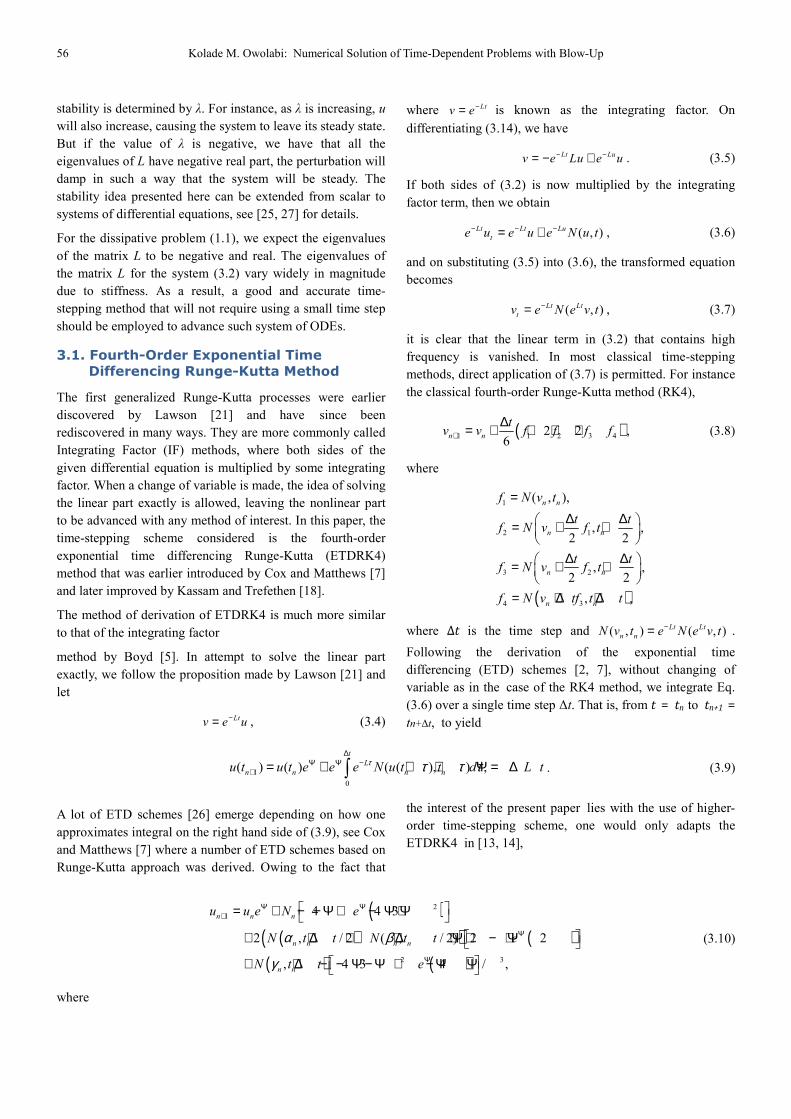
56 Kolade M. Owolabi: Numerical Solution of Time-Dependent Problems with Blow-Up

stability is determined by λ. For instance, as λ is increasing, u

will also increase, causing the system to leave its steady state. But if the value of λ is negative, we have that all the eigenvalues of L have negative real part, the perturbation will damp in such a way that the system will be steady. The stability idea presented here can be extended from scalar to systems of differential equations, see [25, 27] for details.

For the dissipative problem (1.1), we expect the eigenvalues of the matrix L to be negative and real. The eigenvalues of the matrix L for the system (3.2) vary widely in magnitude due to stiffness. As a result, a good and accurate time-stepping method that will not require using a small time step should be employed to advance such system of ODEs.

3.1. Fourth-Order Exponential Time

Differencing Runge-Kutta Method

The first generalized Runge-Kutta processes were earlier discovered by Lawson [21] and have since been rediscovered in many ways. They are more commonly called Integrating Factor (IF) methods, where both sides of the given differential equation is multiplied by some integrating factor. When a change of variable is made, the idea of solving the linear part exactly is allowed, leaving the nonlinear part to be advanced with any method of interest. In this paper, the time-stepping scheme considered is the fourth-order exponential time differencing Runge-Kutta (ETDRK4) method that was earlier introduced by Cox and Matthews [7] and later improved by Kassam and Trefethen [18].

The method of derivation of ETDRK4 is much more similar to that of the integrating factor

method by Boyd [5]. In attempt to solve the linear part exactly, we follow the proposition made by Lawson [21] and let

Ltv e u−= , (3.4)

where Ltv e−= is known as the integrating factor. On differentiating (3.14), we have

Lt Luv e Lu e u− −= − + . (3.5)

If both sides of (3.2) is now multiplied by the integrating factor term, then we obtain

( , )Lt Lt Lu

te u e u e N u t− − −= + , (3.6)

and on substituting (3.5) into (3.6), the transformed equation becomes

( , )Lt Lt

tv e N e v t−= , (3.7)

it is clear that the linear term in (3.2) that contains high frequency is vanished. In most classical time-stepping methods, direct application of (3.7) is permitted. For instance the classical fourth-order Runge-Kutta method (RK4),

( )1 1 2 3 42 26n n

tv v f f f f+

∆= + + + + , (3.8)

where

( )

1

2 1

3 2

4 3

( , ),

, ,2 2

, ,2 2

, ,

n n

n n

n n

n n

f N v t

t tf N v f t

t tf N v f t

f N v tf t t

=∆ ∆ = + +

∆ ∆ = + +

= + ∆ + ∆

where Δt is the time step and ( , ) ( , )Lt Lt

n nN v t e N e v t−= .

Following the derivation of the exponential time differencing (ETD) schemes [2, 7], without changing of variable as in the case of the RK4 method, we integrate Eq. (3.6) over a single time step ∆t. That is, from t = tn to tn+1 =

tn+∆t, to yield

1

0

( ) ( ) ( ( ), ) ,t

L

n n n nu t u t e e e N u t t d L tτ τ τ τ∆

Ψ Ψ −+ = + + + Ψ = ∆∫ . (3.9)

A lot of ETD schemes [26] emerge depending on how one approximates integral on the right hand side of (3.9), see Cox and Matthews [7] where a number of ETD schemes based on Runge-Kutta approach was derived. Owing to the fact that

the interest of the present paper lies with the use of higher-order time-stepping scheme, one would only adapts the ETDRK4 in [13, 14],

( )( )( ) ( )

( ) ( )

21

2 3

4 4 3

2 , / 2 ( , / 2) 2 2

, 4 3 4 / ,

n n n

n n n n

n n

u u e N e

N t t N t t e

N t t e

α β

γ

Ψ Ψ+

Ψ

Ψ

= + − − Ψ + − Ψ + Ψ

+ + ∆ + + ∆ + Ψ + − + Ψ

+ + ∆ − − Ψ − Ψ + − Ψ Ψ

(3.10)

where

International Journal of Bioinformatics and Biomedical Engineering Vol. 1, No. 2, 2015, pp. 53-63 57

( )( ) ( )( ) ( )

/ 2 /2

/2 /2

/ 2 /2

/ ,

, / 2 / ,

2 ( , / 2) / ,

n n n

n n n n

n n n n n

u e e I N L

u e e I N t t L

u e e I N t t N L

α

β α

γ β

Ψ Ψ

Ψ Ψ

Ψ Ψ

= + −

= + − + ∆

= + − + ∆ −

with I defined as the N × N identity matrix, L and N remain the linear and nonlinear

operators, and the functions

2

2 3

1 1 1 / 2( ) , ,

z z z

n n n

e e z e z zz

z z zα β γ− − − − − −= = = .

it is unfortunate that the ETDRK4 scheme suffer from numerical instability as a result of the cancelation errors that are much more pronounced when the eigenvalues of matrix L are close to zero. Cox and Matthews were aware of this problem in their work but managed to play around the computation by using a cutoff point for small eigenvalues. Following [13, 18], the need to seek for a more reliable method is of great interest. One of the initial attempts made to circumvent the vulnerability of these cancelation errors was that of Kassam and

Trefethen [18] by introducing the complex contour integral

1 ( )( )

2

f tf L dt

i tI Lπ Γ=

−∫

to compute the coefficients in the ETDRK4 method at the neighbourhood of the singularity.

This contour integral as suggested and when the involving parameters are carefully chosen has been shown to have improved both stability and accuracy of the scheme. In the present work, we are interested in using the modified ETDRK4 scheme discussed in [13] and present the fourth-order exponential time differencing scheme due to Runge-kutta method as

1 2 1 0

1 2

1 2

2 1

[4 3 ] ( , )

2 [ 2 ] ( , / 2)

2 [ 2 ] ( , / 2)

[ 2 ] ( , ),

n n n n

n n

n n

n n

u u e t N u t

t N t t

t N t t

t N t t

φ φ φφ φ αφ φ β

φ φ γ

Ψ+ = + ∆ Ψ − Ψ + Ψ

+ ∆ Ψ − Ψ + ∆+ ∆ Ψ − Ψ + ∆+ ∆ Ψ − Ψ + ∆

(3.11)

where

/ 20

/ 20 1 1

0 1 1

( / 2) ( / 2) ( , ),

( / 2)[ ( / 2) 2 ( / 2)] ( , ) ( / 2) ( , / 2),

[ 2 ] ( , ) 2 ( , ),

n n n n

n n n n n n

n n n n n n

u e N u t

u e N u t t N t t

u e t N u t h N t t

α φβ φ φ φ αγ φ φ φ γ

Ψ

Ψ

Ψ

= + Ψ Ψ

= + Ψ Ψ − Ψ + ∆ Ψ + ∆

= + ∆ Ψ − Ψ + Ψ + ∆

3.2. Stability Analysis of the ETDRK4 Scheme

Stability region is seen as the parameter region where the amplification is less than or equal to 1. We investigate the linear stability of the ETDRK4 method via linearization of the nonlinear Eq. (3.2)

( ) ( ( ))du

Lu t N u tdt

= + , (3.12)

with Lu(t) and N(u(t)) now represent the linear and nonlinear term. Following [7], we linearize (3.12) about a point u0 that is fixed. That is Lu0 + N(u0) = 0, to yield

( ) ( )du

Lu t u tdt

λ= + , (3.13)

with u, the perturbation to u0 and λ = N’(u0) becomes diagonal or a block diagonal matrix that hosts the eigenvalues of N. For the fixed point u0 to be stable for all λ, then Re(L+λ) < 0.

In the paper, if we adopt a similar technique as employed in [8] and apply the ETDRK4 method to (3.13), one obtains an amplification factor of the form

2 3 410 1 2 3 4( , ) ,n

n

ur x y L L x L x L x L x

u

+ = = + + + + (3.14)

where

2 3 45

1

2 3 45

2

2 3 45

3

2 3 45

4

131 ( ),

2 6 320

1 247 131( ),

2 2 4 2880 57601 61 1441

( ),6 6 720 36 2419201 7 19 25

( ),24 32 640 11520 64512

y y yL y O y

y y y yL O y

y y y yL O y

y y y yL O y

= + + + + +

= + + + + +

= + + + + +

= + + + + +

are the respective asymptotic expansions for Li, i = 1, ..., 4.

It is noticeable at this point to see that the stability curve of ETDRK4 scheme (3.10) coincides with that of the classical RK4 (3.8) as y → 0. It can be shown that

2 6 4

0lim ( , ) 1

2 6 24y

x x xr x y x

→= − + − + ,

58 Kolade M. Owolabi: Numerical Solution of Time-Dependent Problems with Blow-Up

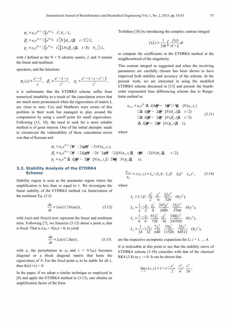
Figure 1. The stability regions of the ETDRK4 method for several negative

values of y in the complex plane x for some values of y.

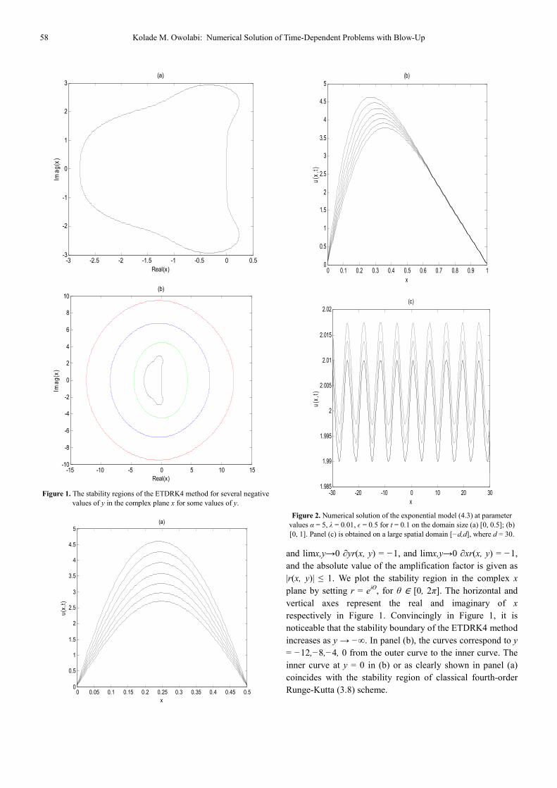
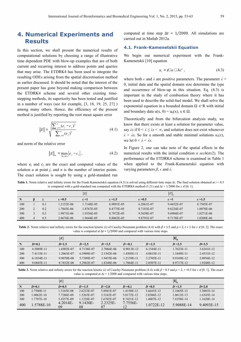
Figure 2. Numerical solution of the exponential model (4.3) at parameter

values α = 5, λ = 0.01, ϵ = 0.5 for t = 0.1 on the domain size (a) [0, 0.5]; (b) [0, 1]. Panel (c) is obtained on a large spatial domain [−d,d], where d = 30.

and limx,y→0 ∂yr(x, y) = −1, and limx,y→0 ∂xr(x, y) = −1, and the absolute value of the amplification factor is given as |r(x, y)| ≤ 1. We plot the stability region in the complex x

plane by setting r = eiϴ, for θ ∈ [0, 2π]. The horizontal and vertical axes represent the real and imaginary of x

respectively in Figure 1. Convincingly in Figure 1, it is noticeable that the stability boundary of the ETDRK4 method increases as y → −∞. In panel (b), the curves correspond to y

= −12,−8,−4, 0 from the outer curve to the inner curve. The inner curve at y = 0 in (b) or as clearly shown in panel (a) coincides with the stability region of classical fourth-order Runge-Kutta (3.8) scheme.

-3 -2.5 -2 -1.5 -1 -0.5 0 0.5-3

-2

-1

0

1

2

3(a)

Real(x)

Ima

g(x

)

-15 -10 -5 0 5 10 15-10

-8

-6

-4

-2

0

2

4

6

8

10(b)

Real(x)

Ima

g(x

)

0 0.05 0.1 0.15 0.2 0.25 0.3 0.35 0.4 0.45 0.50

0.5

1

1.5

2

2.5

3

3.5

4

4.5

5(a)

x

u(x

,t)

0 0.1 0.2 0.3 0.4 0.5 0.6 0.7 0.8 0.9 10

0.5

1

1.5

2

2.5

3

3.5

4

4.5

5(b)

x

u(x

,t)

-30 -20 -10 0 10 20 301.985

1.99

1.995

2

2.005

2.01

2.015

2.02(c)

x

u(x

,t)

International Journal of Bioinformatics and Biomedical Engineering Vol. 1, No. 2, 2015, pp. 53-63 59

4. Numerical Experiments and Results

In this section, we shall present the numerical results of computational solutions by choosing a range of illustrative time dependent PDE with blow-up examples that are of both current and recurring interest to address points and queries that may arise. The ETDRK4 has been used to integrate the resulting ODEs arising from the spatial discretisation method as earlier discussed. It should be noted that the interest of the present paper has gone beyond making comparison between the ETDRK4 scheme and several other existing time-stepping methods, its superiority has been tested and justified in a number of ways (see for example, [3, 18, 19, 25, 27] ) among many others. Hence, the efficiency of the present method is justified by reporting the root mean square error

2

1

2

1

( )

( )

n

j jj

n

jj

e cE

e

=

=

−=∑∑

(4.1)

and norm of the relative error

1max j j

j nE e c

∞ ≤ ≤= − , (4.2)

where ej and cj are the exact and computed values of the solution u at point j, and n is the number of interior points. The exact solution is sought by using a gold-standard run

computed at time step Δt = 1/2000. All simulations are carried out in Matlab 2012a.

4.1. Frank-Kamenetskii Equation

We begin our numerical experiment with the Frank-Kamenetskii [10] equation

u

tu u eε λ= ∇ + , (4.3)

where both ϵ and λ are positive parameters. The parameter λ >

0, initial data and the spatial domain size determine the type and occurrence of blow-up in this situation. Eq. (4.3) is important in the study of combustion theory where it has been used to describe the solid-fuel model. We shall solve the exponential equation in a bounded domain Ω ⊂ R with initial and boundary data u(x, 0) = u0(x), x ∈ Ω.

Theoretically and from the bifurcation analysis study, we know that there exists at least a solution for parameter value, say λs if 0 < λ ≤ λs < ∞, and solution does not exist whenever λ > λs. So for a smooth and stable minimal solutions uλ(x), we let 0 < λ < λs.

In Figure 2, one can take note of the spatial effects in the numerical results with the initial condition α sech(πx2). The performance of the ETDRK4 scheme is examined in Table 1 when applied to the Frank-Kamenetskii equation with varying parameters β, ϵ and λ.

Table 1. Norm relative and infinity errors for the Frank-Kamenetskii equation (4.3) is solved using different time steps ∆t. The final solution obtained at t = 0.5 is compared with a gold-standard run computed with the ETDRK4 method (3.21) and ∆t = 1/2000 for x ∈ [0, 1].

E E∞

N β λ ε =0.5 ε =1 ε =1.5 ε =0.5 ε =1 ε =1.5

100 1 0.1 1.2152E-06 1.7148E-05 6.9891E-05 6.2061E-07 9.4432E-07 8.7505E-07

200 2 0.2 1.7843E-06 1.8767E-05 8.4775E-05 8.7183E-07 9.6224E-07 1.0078E-06 300 3 0.3 1.9871E-06 1.9356E-05 8.7872E-05 9.5658E-07 9.6904E-07 1.0271E-06

400 4 0.5 2.0676E-06 1.9644E-05 8.8062E-05 9.8791E-07 9.7178E-07 1.0208E-06

Table 2. Norm relative and infinity errors for the reaction kinetic (i) of Cauchy-Neumann problem (4.4) with β = 1.5 and p = 2, t = 1 for x ∈ [0, 2]. The exact value is computed at Δt = 1/2000 and compared with various time steps.

E ¥¥¥¥

EEEE

N D=0.1 D=1.5 D =2.5 D =3.5 D =0.1 D =1.5 D =2.5 D=3.5

100 4.5889E-11 1.6902E-07 8.7138E-07 2.7066E-06 8.9013E-12 6.1544E-11 1.7623E-11 3.6241E-12 200 7.4115E-11 1.2063E-07 6.5909E-07 2.1542E-06 1.4505E-11 4.0815E-11 1.1849E-11 2.4531E-12

300 6.1834E-11 9.9070E-08 5.7389E-07 1.9435E-06 1.2139E-11 3.2705E-11 9.9169E-12 2.0956E-12

400 9.0845E-11 8.7432E-08 5.2962E-07 1.8348E-06 1.7864E-11 2.8507E-11 8.9717E-12 1.9248E-12

Table 3. Norm relative and infinity errors for the reaction kinetic (i) of Cauchy-Neumann problem (4.4) with β = 0.5 and p = 2, t =0.5 for x ∈ [0, 1]. The exact value is computed at ∆t = 1/2000 and compared with various time steps.

E ¥¥¥¥

EEEE

N D=0.1 D=0.5 D =1.5 D =2.0 D =0.1 D =0.5 D =1.5 D=2.0

100 2.7580E-11 1.3165E-08 2.6233E-07 5.8941E-07 1.4158E-12 3.6641E-12 2.1065E-13 3.3001E-14 200 1.0062E-10 7.7286E-09 1.5265E-07 3.5242E-07 5.0172E-12 2.0306E-12 1.0613E-13 1.6343E-14 300 1.7707E-10 5.4357E-09 1.1228E-07 2.6702E-07 8.7421E-12 1.4007E-12 7.4358E-14 1.1620E-14

400 1.5788E-10 4.2014E-09

9.1430E-08

2.2325E-07

7.7556E-12 1.0722E-12 5.9088E-14 9.4093E-15

60 Kolade M. Owolabi: Numerical Solution of Time-Dependent Problems with Blow-Up

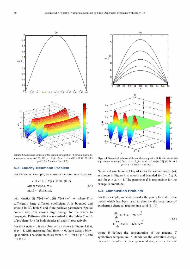
Figure 3. Numerical solution of the semilinear equation (4.4) with kinetic (i) at parameter values (a) D = 0.5, p = 2, β = 2 and t = 3 on [0, 0.5]; (b) D = 0.5,

p = 2, β = 2 and t = 1 on [0, 2].

4.2. Cauchy-Neumann Problem

For the second example, we consider the semilinear equation

( ) (0, ),

(0, ) ( , ) 0,

( ,0) sin( ),

tu D u N u d

u t u d t

u x xβ π

= ∇ + ∈ Ω ×= ==

(4.4)

with kinetics (i) ( ) pN u u= , (ii) ( ) pN u u u= − , where D is

sufficiently large diffusion coefficient, Ω is bounded and smooth in R

N, both β and d are positive parameters. Spatial domain size d is chosen large enough for the waves to propagate. Diffusive effect at is verified in the Tables 2 and 3 of problem (4.4) for both kinetics (i) and (ii) respectively.

For the kinetic (i), it was observed as shown in Figure 3 that, as p > 1, with increasing final time t > 0, there exists a blow-up solution. The solution exists for 0 < t ≤ 1 for all p > 0 and 0 < β ≤ 2.

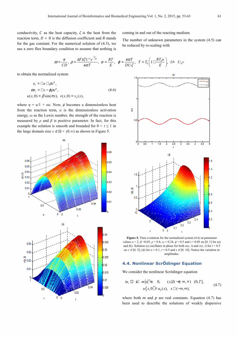
Figure 4. Numerical solution of the semilinear equation (4.4) with kinetic (ii) at parameter values (a) D = 1.5, p = 2, β = 3 and t = 2 on [0, 0.5]; (b) D = 0.5,

p = 3, β = 5 and t = 1 on [0, 3].

Numerical simulations of Eq. (4.4) for the second kinetic (ii), as shown in Figure 4 is smooth and bounded for 0 < β ≤ 5, and for p > 2, t ≤ 1. The parameter β is responsible for the change in amplitude.

4.3. Combustion Problem

For this example, we shall consider the purely local diffusion model which has been used to describe the occurrence of exothermic chemical reaction in a solid [1, 10]

E

p RT

E

p RT

UD U U e

t

TC T U e

t

τ

κ τζ

−

−

∂ = ∇ −∂∂ = ∇ −∂

(4.5)

where U defines the concentration of the reagent, T

symbolizes temperature, E stands for the activation energy, constant τ denotes the pre-exponential rate, κ is the thermal

International Journal of Bioinformatics and Biomedical Engineering Vol. 1, No. 2, 2015, pp. 53-63 61

conductivity, C as the heat capacity, ζ is the heat from the reaction term, D > 0 is the diffusion coefficient and R stands for the gas constant. For the numerical solution of (4.5), we use a zero flux boundary condition to assume that nothing is

coming in and out of the reacting medium.

The number of unknown parameters in the system (4.5) can be reduced by re-scaling with

120

0 0, , , , 1 ,p RT uU e RT T

T T U U vCD T E DU E

ακ ω τζ καω ρ α ϕκα ζ

− = = = = = + =

to obtain the normalized system

0

,

,

( , 0) sin( ), ( ,0) ( ),

t

t

u u e

v v e

u x x v x v x

η

η

ρω ϕρ

β π

= ∇ +

= ∇ −= =

(4.6)

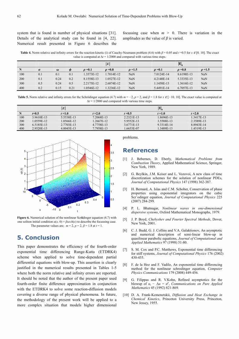
where η = u/1 + αu. Now, ϕ becomes a dimensionless heat from the reaction term, α is the dimensionless activation energy, ω as the Lewis number, the strength of the reaction is measured by ρ and β is positive parameter. In fact, for this example the solution is smooth and bounded for 0 < t ≤ 1 in the large domain size x ∈ Ω × (0,∞) as shown in Figure 5.

Figure 5. Time evolution for the normalized system (4.6) at parameter

values α = 2, β =0.05, ρ = 0.8, ω = 0.24, ϕ = 0.5 and t = 0.05 on [0, 1] for (a) and (b). Solution (c) oscillates in phase for both u(x, t) and v(x, t) for t = 0.5 on x ∈ [0, 5]; (d) for α = 0.1, t = 0.5 and x ∈ [0, 10]. Notice the variation in

amplitudes.

4.4. Nonlinear Scrӧdinger Equation

We consider the nonlinear Scrӧdinger equation

( ) 0

0, ( , ) ( , ) (0, ],

,0 ( ), ( , ),

p

tiu u m u u x t T

u x u x x

+ ∇ + = ∈ −∞ ∞ ×

= ∈ −∞ ∞ (4.7)

where both m and p are real constants. Equation (4.7) has been used to describe the solutions of weakly dispersive

62 Kolade M. Owolabi: Numerical Solution of Time-Dependent Problems with Blow-Up

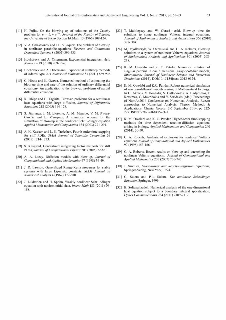
system that is found in number of physical situations [31]. Details of the analytical study can be found in [4, 22]. Numerical result presented in Figure 6 describes the

focussing case when m > 0. There is variation in the amplitudes as the value of β is varied.

Table 4. Norm relative and infinity errors for the reaction kinetic (i) of Cauchy-Neumann problem (4.6) with β = 0.05 and t =0.5 for x ∈ [0, 10]. The exact value is computed at ∆t = 1/2000 and compared with various time steps.

E ¥¥¥¥

EEEE

N α ω ϕ ρ =0.1 ρ =0.8 ρ =1.5 ρ =0.1 ρ =0.8 ρ =1.5

100 0.1 0.1 0.1 1.3573E-12 1.7014E-12 NaN 7.0124E-14 8.6198E-13 NaN

200 0.1 0.24 0.2 8.1558E-13 1.0527E-12 NaN 4.2140E-14 5.3335E-13 NaN 300 0.5 0.24 0.5 2.2175E-12 2.6874E-12 NaN 1.1458E-13 1.3616E-12 NaN

400 0.2 0.15 0.21 1.0546E-12 1.3236E-12 NaN 5.4491E-14 6.7057E-13 NaN

Table 5. Norm relative and infinity errors for the Schrӧdinger equation (4.7) with m = −2, p = 2, and β = 1.8 for x ∈ [−10, 10]. The exact value is computed at ∆t = 1/2000 and compared with various time steps.

E ¥¥¥¥

EEEE

N t=0.5 t =1.0 t =2.0 t =0.5 t =1.0 t =2.0

100 3.9610E-13 5.5538E-13 7.2068E-13 2.2321E-13 1.8696E-13 1.3417E-13 200 1.0559E-12 1.0566E-12 1.2667E-12 5.9552E-13 3.5588E-13 2.3589E-13 300 6.5185E-13 2.7703E-13 4.7758E-13 3.6771E-13 9.3314E-14 8.8943E-14 400 2.9520E-13 4.0045E-13 7.7958E-13 1.6653E-07 1.3489E-13 1.4519E-13

Figure 6. Numerical solution of the nonlinear Scrӧdinger equation (4.7) with one soliton initial condition u(x, 0) = βsech(x) to describe the focussing case.

The parameter values are; m = 2, p = 2, β = 1.8 at t = 1.

5. Conclusion

This paper demonstrates the efficiency of the fourth-order exponential time differencing Runge-Kutta (ETDRK4) scheme when applied to solve time-dependent partial differential equations with blow-up. This assertion is clearly justified in the numerical results presented in Tables 1-5 where both the norm relative and infinity errors are reported. It should be noted that the author of the present paper used fourth-order finite difference approximation in conjunction with the ETDRK4 to solve some reaction-diffusion models covering a diverse range of physical phenomena. In future, the methodology of the present work will be applied to a more complex situation that models higher dimensional

problems.

References

[1] J. Bebernes, D. Eberly, Mathematical Problems from Combustion Theory, Applied Mathematical Science, Springer, New York, 1989.

[2] G. Beylkin, J.M. Keiser and L. Vozovoi, A new class of time discretization schemes for the solution of nonlinear PDEs, Journal of Computational Physics 147 (1998) 362-387.

[3] H. Bernard, A. Islas and C.M. Schober, Conservation of phase properties using exponential integrators on the cubic Scr¨odinger equation, Journal of Computational Physics 225 (2007) 284-299.

[4] P. L. Bhatnagar, Nonlinear waves in one-dimensional dispersive systems, Oxford Mathematical Monographs, 1979.

[5] J. P. Boyd, Chebyshev and Fourier Spectral Methods, Dover, New York, 2001.

[6] C. J. Budd, G. J. Collins and V.A. Galaktionov, An asymptotic and numerical description of semi-linear blow-up in quasilinear parabolic equations, Journal of Computational and Applied Mathematics 97 (1998) 51-80.

[7] S. M. Cox and P.C. Matthews, Exponential time differencing for stiff systems, Journal of Computational Physics 176 (2002) 430-455.

[8] F. de la Hoz and F. Vadilo, An exponential time differencing method for the nonlinear schrodinger equation, Computer Physics Communications 179 (2008) 449-456.

[9] G. Filippas and R. V.Kohn, Refined asymptotics for the blowup of ut − ∆u = up, Communications on Pure Applied Mathematics 45 (1992) 821-869.

[10] D. A. Frank-Kemenetskii, Diffusion and Heat Exchange in Chemical Kinetics, Princeton University Press, Princeton, New Jessey, 1955.

International Journal of Bioinformatics and Biomedical Engineering Vol. 1, No. 2, 2015, pp. 53-63 63

[11] H. Fujita, On the blowing up of solutions of the Cauchy problem for ut = ∆ + u1+α, Journal of the Faculty of Science, the University of Tokyo Section IA Math 13 (1966).109-124.

[12] V. A. Galaktionov and J.L. V´ aquez, The problem of blow-up in nonlinear parabolic.equations, Discrete and Continuous Dynamical Systems 8 (2002) 399-433.

[13] Hochbruck and A. Ostermann, Exponential integrators, Acta Numerica 19 (2010) 209- 286.

[14] Hochbruck and A. Ostermann, Exponential multistep methods of Adams-type, BIT Numerical Mathematic 51 (2011) 889-908.

[15] C. Hirota and K. Ozawa, Numerical method of estimating the blow-up time and rate of the solution of ordinary differential equations- An application to the blow-up problems of partial differential equations

[16] K. Ishige and H. Yagisita, Blow-up problems for a semilinear heat equations with large diffusion, Journal of Differential Equations 212 (2005) 114-128.

[17] S. Jim´enez, I. M. Llorente, A. M. Mancho, V. M. P´erez-Garc´ia and L. V´azquez, A numerical scheme for the simulation of blow-up in the nonlinear Schr¨ odinger equation Applied Mathematics and Computation 134 (2003) 271-291.

[18] A. K. Kassam and L. N. Trefethen, Fourth-order time-stepping for stiff PDEs. SIAM Journal of Scientific Computing 26 (2005) 1214-1233.

[19] S. Krogstad, Generalized integrating factor methods for stiff PDEs, Journal of Computational Physics 203 (2005) 72-88.

[20] A. A. Lacey, Diffusion models with blow-up, Journal of Computational and Applied Mathematics 97 (1998) 39-49.

[21] J. D. Lawson, Generalized Runge-Kutta processes for stable systems with large Lipschitz constants, SIAM Journal on Numerical Analysis 4 (1967) 372-380.

[22] J. Lukkarien and H. Spohn, Weakly nonlinear Schr¨ odinger equation with random initial data, Invent Math 183 (2011) 79-188.

[23] T. Malolepszy and W. Okrasi￣

nski, Blow-up time for solutions to some nonlinear Volterra integral equations, Journal of Mathematical Analysis and Applications 366 (2010) 372- 384.

[24] M, Mydlarczyk, W. Okrasinski and C .A. Roberts, Blow-up solutions to a system of nonlinear Volterra equations, Journal of Mathematical Analysis and Applications 301 (2005) 208-218.

[25] K. M. Owolabi and K. C. Patidar, Numerical solution of singular patterns in one dimensional Gray-Scott-like models, International Journal of Nonlinear Science and Numerical Simulations (2014), DOI:10.1515/ijnsns-2013-0124.

[26] K. M. Owolabi and K.C. Patidar, Robust numerical simulation of reaction-diffusion models arising in Mathematical Ecology. In G. Akrivis, V. Dougalis, S. Gallopoulos, A. Hadjidimos, I. Kotsireas, C. Makridakis and Y. Saridakis (eds.): Proceedings of NumAn2014 Conference on Numerical Analysis. Recent approaches to Numerical Analysis: Theory, Methods & Applications. Chania, Greece; 2-5 September 2014, pp 222-227. ISBN: 978- 960-8475-21-1.

[27] K. M. Owolabi and K. C. Patidar, Higher-order time-stepping methods for time dependent reaction-diffusion equations arising in biology, Applied Mathematics and Computation 240 (2014), 30-50.

[28] C. A. Roberts, Analysis of explosion for nonlinear Volterra equations Journal of Computational and Applied Mathematics 97 (1998) 153-166.

[29] C. A. Roberts, Recent results on blow-up and quenching for nonlinear Volterra equations, Journal of Computational and Applied Mathematics 205 (2007) 736-743.

[30] J. Smoller, Shock-waves and Reaction-diffusion Equations, Springer-Verlag, New York, 1994.

[31] C. Sulem and P.L. Sulem, The nonlinear Schrodinger Equation, Springer, 1999.

[32] B. Soltanalizadeh, Numerical analysis of the one-dimensional heat equation subject to a boundary integral specification, Optics Communications 284 (2011) 2109-2112.