This article was downloaded by: [18.9.61.112] On: 03 November 2016, At: 12:29Publisher: Institute for Operations Research and the Management Sciences (INFORMS)INFORMS is located in Maryland, USA

Operations Research

Publication details, including instructions for authors and subscription information:http://pubsonline.informs.org

Robust Product Line DesignDimitris Bertsimas, Velibor Mišić

To cite this article:Dimitris Bertsimas, Velibor Mišić (2016) Robust Product Line Design. Operations Research

Published online in Articles in Advance 03 Nov 2016

. http://dx.doi.org/10.1287/opre.2016.1546

Full terms and conditions of use: http://pubsonline.informs.org/page/terms-and-conditions

This article may be used only for the purposes of research, teaching, and/or private study. Commercial useor systematic downloading (by robots or other automatic processes) is prohibited without explicit Publisherapproval, unless otherwise noted. For more information, contact permissions@informs.org.

The Publisher does not warrant or guarantee the article’s accuracy, completeness, merchantability, fitnessfor a particular purpose, or non-infringement. Descriptions of, or references to, products or publications, orinclusion of an advertisement in this article, neither constitutes nor implies a guarantee, endorsement, orsupport of claims made of that product, publication, or service.

Copyright © 2016, INFORMS

Please scroll down for article—it is on subsequent pages

INFORMS is the largest professional society in the world for professionals in the fields of operations research, managementscience, and analytics.For more information on INFORMS, its publications, membership, or meetings visit http://www.informs.org

OPERATIONS RESEARCHArticles in Advance, pp. 1–18ISSN 0030-364X (print) � ISSN 1526-5463 (online) https://doi.org/10.1287/opre.2016.1546

© 2016 INFORMS

Robust Product Line Design

Dimitris BertsimasSloan School of Management and Operations Research Center, Massachusetts Institute of Technology, Cambridge, Massachusetts 02139,

dbertsim@mit.edu

Velibor V. MišicAnderson School of Management, University of California, Los Angeles, Los Angeles, California 90095, velibor.misic@anderson.ucla.edu

The majority of approaches to product line design that have been proposed by marketing scientists assume that theunderlying choice model that describes how the customer population will respond to a new product line is known precisely.In reality, however, marketers do not precisely know how the customer population will respond and can only obtain anestimate of the choice model from limited conjoint data. In this paper, we propose a new type of optimization approachfor product line design under uncertainty. Our approach is based on the paradigm of robust optimization where, rather thanoptimizing the expected revenue with respect to a single model, one optimizes the worst-case expected revenue with respectto an uncertainty set of models. This framework allows us to account for parameter uncertainty, when we may be confidentabout the type of model structure but not about the values of the parameters, and structural uncertainty, when we maynot even be confident about the right model structure to use to describe the customer population. Through computationalexperiments with a real conjoint data set, we demonstrate the benefits of our approach in addressing parameter and structuraluncertainty. With regard to parameter uncertainty, we show that product lines designed without accounting for parameteruncertainty are fragile and can experience worst-case revenue losses as high as 23%, and that the robust product line cansignificantly outperform the nominal product line in the worst case, with relative improvements of up to 14%. With regardto structural uncertainty, we similarly show that product lines that are designed for a single model structure can be highlysuboptimal under other structures (worst-case losses of up to 37%), while a product line that optimizes against the worstof a set of structurally distinct models can outperform single model product lines by as much as 55% in the worst caseand can guarantee good aggregate performance over structurally distinct models.

Keywords : product line design; robust optimization; parameter uncertainty; structural uncertainty; model uncertainty.Subject classifications : marketing: choice models, new products.Area of review : Marketing Science.History : Received September 2014; revisions received December 2015, May 2016; accepted June 2016. Published online

in Articles in Advance November 3, 2016.

1. Introduction

A product line is a collection of products that are varia-tions of a single basic product, differing with respect tocertain attributes. Firms offer product lines to account forheterogeneity in consumer preferences. For example, con-sider a producer of breakfast cereals. The basic productmay be a type of cereal (e.g., corn flakes), and a productline may consist of versions of this cereal that differ withrespect to attributes such as the size of the cereal box, theflavor, whether the cereal has low-fat content, whether ithas low-calorie content, whether it is nutritionally enrichedwith certain vitamins, what its retail price is, and so on.The customers of this cereal company may include: weight-conscious adults who may prefer healthy versions of thecereal, college students who may prefer certain flavorsand larger packages (with lower cost per unit weight), orfitness-oriented adults who may prefer enriched cereal thathas added vitamins and minerals in smaller packages andwho may be willing to pay more than other customers. Inthis case, it is clear that there is no single cereal productthat would be highly desirable for all three groups. Rather,

it would be more appropriate to introduce several versionsof the cereal that, taken together, would appeal to all threecategories of customers.

The problem of product line design (PLD) is to select theattributes of the products comprising the product line so asto maximize the revenue that will result from the differenttypes of preferences within the customer population. Thisproblem is one of vital importance to the success of a firm.Much research effort has been devoted to modeling andsolving the PLD problem.

The key prerequisite to practically all existing PLDapproaches is a choice model, which specifies the probabil-ity that a random customer selects one of the products inthe product line or opts to not purchase any of them, giventhe set of products that is offered. Almost all approaches toPLD tacitly assume that this choice model is known pre-cisely and is beyond suspicion. In practice, however, this isnot the case. Typically, the firm can only estimate the modelfrom data that is obtained via conjoint analysis, whereina small number of customers from the overall customerpopulation is asked to either rate or choose from different

1

Dow

nloa

ded

from

info

rms.

org

by [

18.9

.61.

112]

on

03 N

ovem

ber

2016

, at 1

2:29

. Fo

r pe

rson

al u

se o

nly,

all

righ

ts r

eser

ved.

Bertsimas and Mišic: Robust Product Line Design2 Operations Research, Articles in Advance, pp. 1–18, © 2016 INFORMS

hypothetical products. As such, the firm may face signifi-cant uncertainty in the choice model. This uncertainty canbe of the following two types:

1. Parameter uncertainty. For a given parametric choicemodel that fits the data, the firm may be uncertain about thetrue parameter values (e.g., the partworths and the segmentprobabilities) due to the small sample size of the data. Theconcept of parameter uncertainty and the question of howto make decisions under parameter uncertainty have beenwell studied in the operations research community in otherapplications (we survey some of the relevant literature inSection 2), but have received little attention in the contextof product line decisions.

2. Structural uncertainty. For the given conjoint data,the firm may be uncertain about the right type of para-metric model to use to describe the customer population(e.g., a first-choice model or a latent-class multinomial logitmodel). This type of uncertainty is conceptually differentfrom parameter uncertainty, where the focus is restrictedto a single type of model. The concept of structural uncer-tainty is a new one that was recently proposed and stud-ied in Bertsimas et al. (2016) in the context of designingscreening policies for prostate cancer under different mod-els of the evolution of a patient’s health. To the best of ourknowledge, this type of uncertainty has not been consideredpreviously in the context of product line decisions.Uncertainty is of significant interest because the optimalproduct line can change dramatically as one considers dif-ferent parameter values or different structures of the choicemodel. Moreover, a product line that is designed for a par-ticular choice model may result in very different revenues ifthe realized choice model is different from the planned one.

The issue of uncertainty becomes even more significantwhen one considers the nature of product line decisions.A firm’s decision of which products to offer is one that ismade infrequently; in most cases, the decision to producea particular collection of products is one that commits thefirm’s manufacturing, marketing, and operational resourcesand cannot be easily reversed or corrected. This relativelack of recourse, along with the strategic importance of thedecision, underscores the need for a PLD approach thatis immunized to the uncertainty in the underlying choicemodel.

In this paper, we propose a new optimization approachfor PLD that addresses uncertainty in customer choice.Rather than finding the product line that maximizes therevenue under a single, nominal choice model, we proposea robust optimization approach where we specify a set ofpossible models—the uncertainty set—and find the productline that optimizes the worst-case expected revenue, wherethe worst case is taken over all of the models in the uncer-tainty set. We make the following contributions:

1. We propose a new type of PLD problem that accountsfor choice model uncertainty using robust optimization. Ourapproach is flexible in that it is compatible with many exist-ing, popular choice models—such as the first-choice model,

the latent class multinomial logit (LCMNL), model and thehierarchical Bayes mixture multinomial logit (HB-MMNL)model—and we propose different types of uncertainty setsthat account for parametric and structural uncertainty. Wealso discuss how to trade-off nominal and worst-case rev-enue by optimizing a weighted combination of the twotypes of revenues.

2. We demonstrate the value of our approach throughcomputational experiments using a real conjoint data set.In particular:

• We consider parameter uncertainty in the first-choice model, the LCMNL model, and the HB-MMNLmodel. We show that the nominal product line under eachof these types of models is highly vulnerable to parame-ter uncertainty, and that the robust product line providesa significant edge in the worst case. For example, for theLCMNL model with K = 3 customer segments, the rev-enue of the nominal product line drops by more than 10%in the worst case, while the robust product line leads toworst-case revenues that are 4% higher than the nominalproduct line.

• We consider structural uncertainty through twoexamples. In the first example, we consider an uncertaintyset of LCMNL models where the models vary in terms ofthe number of segments K; here, we find that the nominalproduct line under any one LCMNL model can result in aworst-case revenue that is lower than the nominal revenueby 3%–7%, while the robust product line outperforms thenominal product lines in the worst case by 2%–4%. In thesecond example, we consider an uncertainty set that con-sists of LCMNL models and the first-choice (FC) model.Here, we find that the LCMNL models and the FC modellead to strikingly different product lines, and the productline that is optimal for each individual model is highlysuboptimal under the other models. In contrast, the robustproduct line that accounts for all of the structurally distinctmodels outperforms each nominal product line under theworst-case model.

The rest of the paper is organized as follows. In Sec-tion 2, we review the existing literature on PLD. InSection 3, we describe our PLD approach to addressuncertainty in customer choice. In Section 4, we presentextensive computational evidence that highlights the needto account for uncertainty and the benefits of adopting ourapproach to address uncertainty. Finally, in Section 5, weconclude the paper and discuss some possible directions forfuture work.

2. Literature Review

To date, significant research has been conducted in solv-ing the PLD problem. The majority of approaches to thePLD problem model it as an integer optimization prob-lem and assume a first-choice model of customer behav-ior; examples include Zufryden (1982), Green and Krieger(1985), McBride and Zufryden (1988), Dobson and Kalish

Dow

nloa

ded

from

info

rms.

org

by [

18.9

.61.

112]

on

03 N

ovem

ber

2016

, at 1

2:29

. Fo

r pe

rson

al u

se o

nly,

all

righ

ts r

eser

ved.

Bertsimas and Mišic: Robust Product Line DesignOperations Research, Articles in Advance, pp. 1–18, © 2016 INFORMS 3

(1988), Kohli and Sukumar (1990), and Dobson and Kalish(1993). The approaches differ in whether the procedureselects the product line from a predefined set of products(“product space” procedures; examples include Green andKrieger 1985; McBride and Zufryden 1988; Dobson andKalish 1988, 1993) or whether the procedure directly pre-scribes the attributes and is not restricted to a predefined set(“attribute space” procedures; examples include Zufryden1982, Kohli and Sukumar 1990). The approaches also dif-fer in the solution method. For example, Zufryden (1982)and McBride and Zufryden (1988) solve their respectivePLD problems exactly as integer optimization problems,while Green and Krieger (1985) consider several heuris-tics, including a greedy heuristic and Kohli and Sukumar(1990) consider a dynamic programming-based heuristic.For a comprehensive comparison of heuristics for the nom-inal first-choice PLD problem, the reader is referred to thepaper of Belloni et al. (2008).

Apart from the first-choice model, other product lineresearch has considered probabilistic choice models, suchas the multinomial logit (MNL) model, where customersdo not deterministically select their highest utility choice,but rather they randomly select from all of their choices;typically, options with higher utilities are selected more fre-quently. Examples of product line approaches built on prob-abilistic choice models include Chen and Hausman (2000),Kraus and Yano (2003), Schön (2010a, 2010b). In Chenand Hausman (2000), the authors consider the problem ofselecting a product line from a finite set of products to max-imize expected revenue under the MNL model. Althoughthe problem belongs to the class of mixed-integer nonlinearoptimization problems, which are typically very difficultto solve, the paper shows that due to the problem struc-ture, it is sufficient to solve the continuous relaxation toobtain an optimal solution to the original problem. Schön(2010a) builds on this modeling approach to incorporateprice discrimination for different customer segments, whileSchön (2010b) further extends the approach to more gen-eral attraction models. Kraus and Yano (2003) consider ashare-of-surplus choice model, where the probability of asegment selecting a product is the ratio of the surplus ofthat product to the total surplus over all of the products.The problem they formulate is a mixed-integer nonlin-ear optimization problem, which they solve with a combi-nation of simulated annealing and steepest ascent. Krausand Yano (2003) also additionally address uncertainty inthe utilities by modeling the uncertain utilities as randomvariables and applying a heuristic that attempts to opti-mize the expected profit. Outside of the academic literature,Sawtooth Software’s Advanced Simulation Module (ASM)(Sawtooth Software 2003) allows analysts to perform sim-ulations and to find product lines that optimize one of anumber of objectives (such as market share or revenue)with respect to different choice models. These choice mod-els include the first-choice model, the MNL model, and therandomized first-choice (RFC) model. The RFC model is a

type of probabilistic choice model, wherein one simulatesmany customers who choose according to the first-choicerule with a randomly generated utility function; the prod-uct utilities are altered for each customer by perturbing thepartworths (“attribute error”) and then perturbing the utilityof each product (“product error”).

The approach we propose in this paper differs fromthe extant PLD literature in two main ways. First, exist-ing approaches to the PLD problem under the first-choicemodel and under probabilistic choice models assume thatthe choice model that describes the customer population isknown precisely. For example, in the first-choice model,it is assumed that we precisely know the segments com-prising the customer population along with their partworthsand sizes. As discussed earlier, typically the parameter val-ues that define the choice model may not be known withcomplete certainty. As we will show later, product linesthat do not account for errors in the parameter values thatdefine the choice model can lead to significantly lowerrevenues when the realized parameter values are differentfrom their planned values. To the best of our knowledge,no other work has highlighted the importance of account-ing for parameter uncertainty in PLD or proposed a PLDapproach that directly accounts for this uncertainty. Closestin spirit to some of the analyses we conduct is part of thepaper of Belloni et al. (2008), where the authors presenta post hoc test of how robust the product lines are withrespect to error in the partworth utilities. In this experi-ment, the firm observes partworths that are perturbed fromthe true partworths (to simulate measurement error) anddesigns the product line under the perturbed partworths;the authors show that in this setting, the realized revenuesare 2%–5% lower than their anticipated values due to thismeasurement error. In this paper, we consider uncertaintymore generally over a wide range of choice models (thefirst-choice model, the LCMNL model, and the HB-MMNLmodel) and propose an approach that accounts for uncer-tainty upfront; as such, our paper complements this existingset of results. With regard to the RFC model implementedin Sawtooth Software’s ASM, we emphasize that the RFCmodel addresses randomness in choice in the same waythat other probabilistic choice models do; attribute error isanalogous to assuming a probability distribution over part-worths (as in the LCMNL model, which assumes a dis-crete mixture distribution or the HB-MMNL model, whichassumes a multivariate normal mixture distribution), andproduct error is analogous to utility error in a random utilityframework (as in the MNL model, which assumes standardGumbel errors, or the multinomial probit model, whichassumes normally distributed errors). The RFC model doesnot address uncertainty in a worst-case way, as we do inthe present paper.

Second, virtually all existing approaches to the PLDproblem focus on a single parametric structure for thechoice model. In contrast, our approach is also designed toaccommodate structural uncertainty and account for multi-ple parametric structures. The motivation for this setting is

Dow

nloa

ded

from

info

rms.

org

by [

18.9

.61.

112]

on

03 N

ovem

ber

2016

, at 1

2:29

. Fo

r pe

rson

al u

se o

nly,

all

righ

ts r

eser

ved.

Bertsimas and Mišic: Robust Product Line Design4 Operations Research, Articles in Advance, pp. 1–18, © 2016 INFORMS

that often we may not be able to isolate a single paramet-ric model as the “best” model, but instead we may havea collection of models that are “good enough” and thatcould all plausibly describe how the customer populationwill respond to the product line. The danger of optimizingfor a single model is that we do not take the other modelsinto consideration: while the single model product line willguarantee the optimal revenue under the chosen model, itis not guaranteed to deliver good performance under any ofthe other models. Thus, in our approach, rather than usinga single model, we account for all of the models by opti-mizing a product line with respect to worst-case revenueover the set of models. In this way, the product line isable to guarantee good performance over a range of mod-els, rather than only guaranteeing good performance for asingle model. To the best of our knowledge, the idea ofoptimizing for a set of structurally distinct models has notbeen proposed in the PLD literature.

The preceding discussion has focused on PLD underuncertainty in the underlying choice model; it is worth not-ing that other research has considered PLD under otherforms of uncertainty. One such uncertainty is engineeringuncertainty, where the products must be designed so thatthey meet certain engineering specifications under varyinguse conditions; see, for example, Luo (2011). Although wedo not consider the engineering aspect of PLD or engi-neering uncertainty in this paper, it would be interesting toconsider in future research.

A related problem to PLD is the single product design(SPD) problem, where the firm seeks to design a singleproduct as opposed to a collection of products; for anoverview of the SPD literature, the reader is referred to theliterature review of Luo (2011). Within the SPD literature,the papers of Luo et al. (2005) and Besharati et al. (2006)consider robustness in the SPD problem from an inte-grated engineering and marketing perspective and, in par-ticular, they consider uncertainty in consumer preferencesthat arises from uncertainty in engineering parameters (forexample, consumers may have different use requirementsfor the product, which can lead to variations in the prod-uct’s utility), as well as small conjoint sample sizes. Thelatter form of uncertainty is related to the parameter uncer-tainty that we study in the present paper and as such,our paper complements this existing work in presenting amethodology for addressing parameter uncertainty in pref-erences in the design of product lines, as opposed to sin-gle products. Our paper is further differentiated from thisexisting work in robust SPD by also considering structuraluncertainty in preferences, which is not considered in Luoet al. (2005) and Besharati et al. (2006).

Outside of the PLD literature, our treatment of param-eter uncertainty is closely aligned with the large body ofwork within the operations research community on robustoptimization (Bertsimas et al. 2011). Robust optimization isa technique for optimization under uncertainty, where onewishes to solve an optimization problem that is affected

by uncertainty either through its constraints or its objec-tive function. Robust optimization has been successfullyapplied in a variety of domain areas to address parame-ter uncertainty, including inventory management (Bertsimasand Thiele 2006), portfolio optimization (Bertsimas andSim 2004, Goldfarb and Iyengar 2003), power system oper-ations (Bertsimas et al. 2013), and facility location deci-sions (Baron et al. 2011). The only application of robustoptimization techniques to a problem involving paramet-ric choice models that we know of is the paper of Rus-mevichientong and Topaloglu (2012). In this paper, theauthors consider the problem of assortment optimization—a problem closely related to PLD—under the MNL modelwith uncertain utilities. They develop theoretical resultsthat show that the robust MNL assortment problem canbe solved efficiently; in particular, there exists a revenue-ordered assortment that is optimal, and therefore one canfind the globally optimal assortment by enumerating N dif-ferent assortments, where N is the number of products. Ourpaper contrasts with this work in a number of ways. First,our paper considers parameter uncertainty under a broadercollection of choice models, namely, the first-choice model,the latent class MNL model, and the hierarchical Bayesmixture MNL model. Second, the theoretical results that aredeveloped in Rusmevichientong and Topaloglu (2012) aretailored to the MNL model; in contrast, the uncertainty setsthat we propose and the algorithm that we adapt to solvethe robust problem (the divide-and-conquer algorithm; seeGreen and Krieger 1993, Belloni et al. 2008) are generalpurpose and can be used to address parameter uncertaintyin a wide range of choice models. Finally, our paper alsoconsiders structural uncertainty, where the uncertainty canrange over different parametric model structures, which isnot considered in Rusmevichientong and Topaloglu (2012).

Our treatment of structural uncertainty was inspired bythe paper of Bertsimas et al. (2016). The paper consid-ers the problem of selecting a prostate cancer screeningstrategy to maximize a patient’s expected quality adjustedlife years. This problem is made difficult by the existenceof three distinct, yet clinically recognized, models of howa patient’s health evolves under different screening strate-gies. To reconcile these different models, the authors pro-pose optimizing a weighted combination of the worst-casepatient outcome and the average outcome over the threemodels. The authors show that the resulting screening strat-egy leads to good outcomes under all three models andis superior to the single-model screening strategies in itsworst- and average-case performances. The results in thepresent paper complement those in Bertsimas et al. (2016)by showing that this idea can have significant impact inproduct line decisions.

3. Model

3.1. Nominal Model

Let n be the number of different attributes of the product.We assume, for simplicity, that each attribute is a binary

Dow

nloa

ded

from

info

rms.

org

by [

18.9

.61.

112]

on

03 N

ovem

ber

2016

, at 1

2:29

. Fo

r pe

rson

al u

se o

nly,

all

righ

ts r

eser

ved.

Bertsimas and Mišic: Robust Product Line DesignOperations Research, Articles in Advance, pp. 1–18, © 2016 INFORMS 5

attribute, i.e., either the product possesses the attributeor not. (This assumption is without loss of generality, asattributes with more than two levels can be modeled by,for example, introducing a binary attribute for each levelof the original attribute and requiring that the product onlypossesses one of the binary attributes.) A product is thena binary vector a = 4a11 a21 0 0 0 1 an5. We let N denote thenumber of candidate products and we index these productsfrom 1 to N ; for p ∈ 811 0 0 0 1N 9, ap indicates the attributevector that encodes product p.

We assume that the marginal revenue of product p isgiven by r4p5. To model the market, we assume that eachcustomer makes exactly one choice: he either chooses oneof the products in the product line, or he chooses a “no-purchase” option, which corresponds to not purchasing aproduct from the product line (e.g., because of the exis-tence of a more desirable product by a competing firm).The purchasing behavior of customers is described by achoice model m; the quantity m4p �S5 denotes the proba-bility that the customer selects product p when offered theproduct line S ⊆ 811 0 0 0 1N 9. We use the index 0 to indi-cate the no-purchase option, so that m40 � S5 denotes theprobability that the customer does not purchase any of theproducts in S. The expected revenue of product line S isthen given by

R4S3m5=∑

p∈S

m4p � S5 · r4p50 (1)

Let P be the number of products that are to compose theproduct line (the “width” of the product line). We assumethat P is predefined by the firm and is not a decision vari-able. The nominal PLD problem can then be stated as

maximizeS⊆8110001N 92 �S�=P

R4S3m50 (2)

In words, this is the problem of finding a product lineS consisting of P products from the universe of products811 0 0 0 1N 9 that leads to the highest possible expected rev-enue under the choice model m.

There are many possible choices for the choice modelm; we present three examples as follows:

1. First-choice. We assume that there are finitely manycustomer types; let K denote the number of customer types.We assume that K is predefined by the firm and is not adecision variable. We let �k denote the probability that arandom customer is of type k. We thus have that

∑Kk=1 �

k =

1 and �k ¾ 0 for all k ∈ 811 0 0 0 1K9. For each customer-typek ∈ 811 0 0 0 1K9, we let uk4p5 denote the utility of productp ∈ 811 0 0 0 1N 9 and we let uk405 denote the utility of the no-purchase option for type k. We assume that the utilities areunique: if p 6= p′, then uk4p5 6= uk4p′5, i.e., two productscannot have the same utility. Such an assumption is help-ful in ensuring that the first-choice model is well defined.Given that the products are defined by discrete attributes,this assumption is not particularly restrictive.

With these definitions, the choice probability m4p �S5can be defined as

m4p � S5=

K∑

k=1

�k·

{

p = arg maxp′∈S∪809

uk4p′5

}

1 (3)

and the expected revenue R4S3m5 is just

R4S3m5=∑

p∈S

( K∑

k=1

�k· {

p = arg maxp′∈S∪809

uk4p′5}

)

· r4p50 (4)

We assume (as is commonly done in conjoint analysis) thatthe utility of a product p is a linear function of its attributes;that is,

uk4p5=

n∑

i=1

uki · a

pi 1 (5)

where uki is the partworth utility of attribute i for customer-

type k. We will use u to denote the vector of attributepartworths, i.e., uk = 4uk

11 0 0 0 1 ukn5.

2. Latent class multinomial logit. We now define thelatent class multinomial logit (LCMNL) model. As in thefirst-choice model, we assume that there are K customersegments. A customer belongs to segment k with probabil-ity �k. Each product p ∈ 811 0 0 0 1N 9 provides some utilityuk4p5 to customers in segment k and as before, we assumethat uk405 is the utility of the no-purchase option. Thechoice probability m4p � S5 is then given by

m4p � S5=

K∑

k=1

�k exp4uk4p55∑

p′∈S exp4uk4p′55+ exp4uk4055(6)

and the expected revenue under m is given by

R4S3m5=∑

p∈S

K∑

k=1

�k r4p5 · exp4uk4p55∑

p′∈S exp4uk4p′55+ exp4uk40550 (7)

As in the first-choice model, we will assume that the utilityuk4p5 is a linear function of the attributes of product p (cf.Equation (5)) and use u to denote the vector of attributepartworths, i.e., uk = 4uk

11 0 0 0 1 ukn5.

3. Mixture multinomial logit. In the mixture multinomiallogit (MMNL) model, we assume that customers chooseaccording to an MNL model, where the partworth vectoru = 4u11 0 0 0 1 un5 is distributed according to some mixturedistribution F . The choice probabilities are then given by

mF 4p � S5=

∫ exp4u4p55∑

p′∈S exp4u4p′55+ exp4u4055dF 4u51 (8)

where u4p5 is the utility of product p under the partworthvector u. Note that when F is a distribution with finite sup-port, the choice model reduces to the LCMNL model (6).It is common to assume that u is normally distributed withmean  and covariance matrix V. Thus, given  and V, thecorresponding choice probability can be written as

mÂ1V4p � S5 =

∫ exp4u4p55∑

p′∈S exp4u4p′55+ exp4u4055

·�4u3Â1V5du1 (9)

Dow

nloa

ded

from

info

rms.

org

by [

18.9

.61.

112]

on

03 N

ovem

ber

2016

, at 1

2:29

. Fo

r pe

rson

al u

se o

nly,

all

righ

ts r

eser

ved.

Bertsimas and Mišic: Robust Product Line Design6 Operations Research, Articles in Advance, pp. 1–18, © 2016 INFORMS

where �4·3Â1V5 is the density function of a multivari-ate normal random variable with mean  and covariancematrix V.

Assuming a mixture distribution that is a multivariatenormal, there are two approaches to estimating  and V.The first approach is based on expectation maximization(EM) (see Train 2009, 2008), which produces point esti-mates of  and V. The second approach, which is morepopular in marketing science and is more widely used inpractice, is based on a hierarchical Bayes (HB) formulationof the model (Allenby and Rossi 1998, Rossi and Allenby2003, Rossi et al. 2012). In the HB approach,  and V aretreated as random variables with prior distributions, and thegoal is to compute the posterior distributions of  and Vgiven the available choice data from a conjoint analysis ofa group of respondents. One of the most common spec-ifications of the parameter priors (see Allenby and Rossi1998, Rossi et al. 2012) is given by

Â∼N4Â1�V51 (10a)

V ∼ IW4v01V051 (10b)

where N4Ì1è5 indicates a multivariate normal distributionwith mean Ì and covariance matrix è and IW4�1W5 indi-cates the inverse Wishart distribution with degrees of free-dom � and scale matrix W. Typically, the parameters of thepriors of  and V are specified to ensure that the priors arerelatively diffuse. In what follows, we will use HB-MMNLto denote the MMNL model with the above hierarchicalBayes specification (Equations (10a) and (10b)).

Letting ë denote the posterior joint probability densityfunction of 4Â1V5, it is common to compute the posteriormean of the choice probability mÂ1V4p � S5 (i.e., by inte-grating mÂ1V4p � S5 over ë ), and to use this as the choiceprobability:

m4p �S5 =

∫ ∫ exp4u4p55∑

p′∈S exp4u4p′55+exp4u4055·�4u3Â1V5

·ë4Â1V5 dudÂdV0 (11)

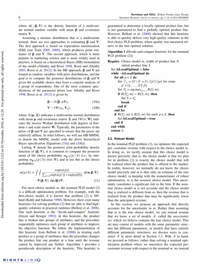
For most choice models m, the nominal PLD model (2)is a difficult optimization problem. For example, with thefirst-choice model, it is known that problem (2) is NP-hard (Kohli and Sukumar 1990). However, there exist manyheuristics for solving problem (2) that are able to find high-quality solutions in practical runtimes (Belloni et al. 2008).One such heuristic is the “divide-and-conquer” heuristic(Green and Krieger 1993). In this heuristic, the productline is broken into groups of attributes, and the proceduresequentially optimizes each group of attributes to improvethe objective function. We follow the implementation ofthis heuristic from Belloni et al. (2008) in treating eachproduct as a group of attributes; thus the procedure changesthe product line one product at a time until the revenuecannot be improved any further. Algorithm 1 provides apseudocode description of the heuristic. This heuristic is

guaranteed to determine a locally optimal product line, butis not guaranteed to find a globally optimal product line.However, Belloni et al. (2008) showed that this heuristicis able to quickly deliver very high-quality solutions in thefirst-choice PLD problem, where quality was measured rel-ative to the true optimal solution.

Algorithm 1 (Divide-and-conquer heuristic for the nominalPLD problem (2)).Require: Choice model m, width of product line P ,

initial product line SSet isLocalOptimal = falsewhile ¬isLocalOptimal do

for all p ∈ S doSet Sp = 8S ′ � S ′ = S ∪ 8p′9\8p9 for somep′ ∈ 811 0 0 0 1N 9\S9

Set S∗p = arg maxS∈Sp

R4S3m5

if R4S∗p3m5 >R4S3m5, then

Set S = S∗p

breakend if

end forif R4S∗

p3m5¶R4S3m5 for each p ∈ S, thenSet isLocalOptimal = true

end ifend whilereturn S.

3.2. Robust Model

In the nominal PLD problem (2), we optimize the expectedper -customer revenue with respect to the choice model m.In doing so, we tacitly assume that this choice model isknown precisely; that is, the choice model m that we planfor in problem (2) is exactly the choice model that willbe realized when the product line is offered to the market.In reality, however, we normally do not know the choicemodel precisely and m is thus only an estimate of the truechoice model; in keeping with the nomenclature of robustoptimization, m is the nominal choice model. This uncer-tainty constitutes a significant risk to the firm. If the nom-inal choice model m is not accurate and the choice modelthat is realized is different from m, then the revenue that isrealized from the product line may be significantly lowerthan the anticipated revenue.

In this section, we propose an approach that directlyaccounts for the uncertainty in m. Rather than assumingthat m is the true choice model, we can instead assumethat we know a set of models M, called the uncertaintyset, which we believe contains the true choice model. Thisset may consist of models with the same parametric struc-ture but different parameters, or models that have entirelydifferent parametric structures; we discuss ways to con-struct M in more detail in Section 3.3. With M in hand,we proceed as follows: rather than solving a nominal opti-mization problem where we maximize the expected per-customer revenue with respect to the nominal m, we instead

Dow

nloa

ded

from

info

rms.

org

by [

18.9

.61.

112]

on

03 N

ovem

ber

2016

, at 1

2:29

. Fo

r pe

rson

al u

se o

nly,

all

righ

ts r

eser

ved.

Bertsimas and Mišic: Robust Product Line DesignOperations Research, Articles in Advance, pp. 1–18, © 2016 INFORMS 7

solve a robust optimization problem where we maximizethe worst-case expected per-customer revenue, where theworst case is taken over all the possible choice models min the uncertainty set M. Mathematically, the worst-caseexpected revenue of a product line S is defined as

R4S3M5= minm∈M

R4S3 m50 (12)

i.e., the worst-case expected per-customer revenue is theminimum of the expected per-customer revenue overthe possible choice models in M. It is helpful to think of mas being controlled by an adversary (“nature”) that wishesto reduce the expected per-customer revenue that the deci-sion maker garners; given the freedom to choose any mfrom M, nature will select the one that makes the expectedper-customer revenue the lowest. For further backgroundin robust optimization, the reader is referred to the reviewpaper of Bertsimas et al. (2011).

The robust PLD problem can then be defined as

maximizeS⊆8110001N 92 �S�=P

R4S3M50 (13)

Note that, like the nominal PLD problem (2), the robustPLD problem (13) is still, in general, a difficult problem tosolve to provable optimality. However, many of the sameheuristics that are available for solving the nominal PLDproblem (2) can be used to solve this problem. In particular,we can use the divide-and-conquer heuristic (Algorithm 1)to solve the problem, where we replace evaluations of thenominal objective function R4·3m5 with evaluations of theworst-case objective function R4·3M5.

Before we describe the possible forms of the uncertaintyset M, it is worthwhile to highlight three important aspectsof the robust model. First, we would like to provide somefurther motivation for the objective in problem (13). Theobjective function (12) still considers the expected revenueof the product line, but unlike the nominal objective func-tion (1), it considers the worst-case expected profit of theproduct line, where the worst case is taken over the uncer-tainty set M of choice models. As discussed in Section 2,this contrasts with existing approaches to the PLD problem,all of which consider maximizing expected revenue or mar-ket share under a single nominal choice model. The reasonfor taking our view is that each model in M represents aplausible outcome with regard to how the customer popula-tion might react to the product line and thus, for a productline S, the set 8R4S3 m5 � m ∈ M9 represents a set of pos-sible outcomes in terms of the expected per-customer rev-enue. Different product lines will differ in terms of the setof possible revenue outcomes they induce. A low revenueoutcome may have significant negative consequences forthe firm’s financial viability and its perceived performance.Thus, rather than ensuring a good average revenue outcomeover the models in M, the firm may wish to ensure a goodrevenue outcome under the least favorable model. To illus-trate this, consider Figure 1, which displays the hypotheti-cal expected per-customer revenue distributions induced by

Figure 1. (Color online) Hypothetical illustration ofrevenue distributions under two differentproduct lines.

0

0.1

0.2

50 55 60 65

Revenue

Den

sity

Solution

Product line A

Product line B

a set of choice models M for two different product lines.The dashed vertical line indicates a target value for theexpected per-customer revenue. Here, we can see that whileproduct line A ensures a better average performance overthe models in M than product line B, there are many out-comes where the revenue under product line A is below thetarget revenue, as indicated by the much heavier tail belowthe target revenue. Thus, in this setting, product line B maybe more desirable to the firm than product line A. This isthe typical behavior observed when comparing nominal androbust product lines (here, product line A’s revenue distri-bution is representative of that of a nominal product line,while product line B is representative of the robust productline).

The second aspect concerns how the solutions of thenominal problem (2) and the robust problem (13) relate toeach other in terms of expected per-customer revenue. LetSN be an optimal collection of products for the nominalproblem (2) and let SR be an optimal collection of productsfor the robust problem (13) with uncertainty set M. Then,it follows that the worst-case expected per-customer rev-enue of the robust solution is always at least as good as theworst-case expected per-customer revenue of the nominalsolution; that is,

R4SR3M5¾R4SN3M50

To see this, observe that SN is a feasible solution for prob-lem (13); since SR is an optimal solution for problem (13),it follows that SN cannot have a higher value of R4·3M5 asthis would contradict the optimality of SR for problem (13).A similar result follows in the other direction with respectto the nominal expected per-customer revenue: the nomi-nal expected per-customer revenue of the nominal solutionis always at least as good as the nominal expected per-customer revenue of the robust solution; that is,

R4SR3m5¶R4SN3m50

Dow

nloa

ded

from

info

rms.

org

by [

18.9

.61.

112]

on

03 N

ovem

ber

2016

, at 1

2:29

. Fo

r pe

rson

al u

se o

nly,

all

righ

ts r

eser

ved.

Bertsimas and Mišic: Robust Product Line Design8 Operations Research, Articles in Advance, pp. 1–18, © 2016 INFORMS

In summary: the robust solution will perform better thanthe nominal solution in the worst case, while the nominalsolution will perform better than the robust solution in thenominal case.

The third aspect of the robust model that is importantto consider is the form and the size of the uncertainty set.As the size of the uncertainty set M increases, the mini-mization in (12) is taken over a larger set, and thus thecorresponding solution of problem (13) will ensure the bestworst-case performance over a larger set of possible valuesof m. However, as the uncertainty set increases in size, typ-ically, the performance of the robust solution in the nominalcase degrades. Thus, there is a trade-off in selecting theuncertainty set: if the set is too large and contains modelsm that are significantly different from the nominal modelm, then the robust solution will be protected against theserealizations (relative to the nominal solution), but at thecost of performance under the nominal model m. In con-trast, if the set is too small, then the robust solution willhave better performance under the nominal model m, butwill be vulnerable to extreme realizations of m.

3.3. Choices of the Uncertainty Set

We now discuss some ways that we may generate theuncertainty set M.

1. Finite set of variations of a single model. Supposethat we fix a given type of model—for example, a latent-class multinomial logit model with K classes. We may thengenerate B different versions of the same type of model,leading to the uncertainty set

M= 8m11 0 0 0 1mB90 (14)

These variations could be generated in a number of ways:(a) Bootstrapping. We may generate B bootstrapped

samples of the conjoint data by sampling with replacementfrom the respondents in the data set. We can then run theestimation procedure of our desired model class on thechoice data of each bootstrapped sample, thus generatingB different models.

(b) Posterior sampling. Bayesian models like HB willfurnish us with a posterior distribution of a parameter È thatspecifies the model; for example, in the MMNL model inEquation (9), the underlying model is specified by the meanand covariance matrix pair 4Â1V5, and in estimating themodel, one computes the posterior distribution of 4Â1V5.In a Bayesian setting, the parameter È is unknown, and ouruncertainty in this parameter is captured in the posteriordistribution of È given the available choice data. To formM, we may therefore take B independent samples from theposterior distribution of È—say, È11 0 0 0 1ÈB—and set eachmb to be the choice model with parameter Èb.

(c) Multiple models from the estimation procedure. Itmay be the case that the estimation procedure generatesmultiple models from the same data. For example, the EM

procedure (Dempster et al. 1977), which is the typical esti-mation method of choice for latent-class multinomial logitmodels and other popular discrete choice models, may con-verge to B different local minima given different initialstarting points that are similar in their log likelihood.

2. Continuous set of variations of a single model. Ratherthan considering a finite collection of B different versionsof the same model, we may want to consider sets where oneor more parameters that define the model vary continuouslywithin some set. Letting È denote the parameter, ä denotethe set of possible values of È and mÈ denote the modelthat corresponds to È, M will be defined as

M= 8mÈ � È ∈ä91 (15)

and correspondingly, R4S3M5 will be defined as

R4S3M5 = minm∈M

R4S3 m5

= minÈ∈ä

R4S3mÈ50 (16)

In the previous choice of the uncertainty set M, wherethe uncertainty set M consists of finitely many models,the worst-case revenue R4S3M5 can be easily computed:simply compute R4S3m5 under each of the finitely manymodels m in M and take the minimum of this set of Bvalues. In contrast, when the uncertainty set M consists ofinfinitely many models, the function R4S3M5 may not beeasy to evaluate. As shown in Equation (16), the difficultyof computing R4S3M5 depends on how hard it is to opti-mize R4S3mÈ5 as a function of the parameter È over theset of possible parameter values ä.

One broad case where R4S3M5 is easy to compute iswhen R4S3mÈ5 is a linear function of È and ä is a polyhe-dron (that is, a set defined by finitely many linear equalitiesand inequalities on È). In this case, R4S3M5 can be com-puted by solving a linear optimization problem, which is atheoretically tractable problem; this can also be done effi-ciently in practice provided that the dimension of È andthe number of constraints defining ä are not too large. Anexample of such a case is when we consider uncertainty incustomer-type probabilities in the first-choice model. Moreconcretely, we assume that the customer-type probabilitydistribution Ë is uncertain and belongs to some polyhedralset å. Letting mË denote the first-choice model with prob-ability distribution Ë, we can write

R4S3M5=minË∈å

R4S3mË5

=minË∈å

K∑

k=1

�k

(

∑

p∈S

{

p=argmaxp′∈S∪809

uk4p′5}

·r4p5

)

0 (17)

In Equation (17), we can see that the function being mini-mized is linear in Ë, and thus computing R4S3M5 amountsto solving a linear optimization problem. We now presenttwo choices for the parameter uncertainty set å:

(a) Box uncertainty set. We assume that for each seg-ment k, �k is restricted to lie between �k and �k. The box

Dow

nloa

ded

from

info

rms.

org

by [

18.9

.61.

112]

on

03 N

ovem

ber

2016

, at 1

2:29

. Fo

r pe

rson

al u

se o

nly,

all

righ

ts r

eser

ved.

Bertsimas and Mišic: Robust Product Line DesignOperations Research, Articles in Advance, pp. 1–18, © 2016 INFORMS 9

uncertainty set åbox is then given by

åbox =

Ë∈�K

∣

∣

∣

∣

∣

∣

�k¶ �k¶ �k1 ∀k∈8110001K91

1T Ë=11˾00

(18)

(b) Aggregate deviation uncertainty set. A limitationof the box uncertainty set is that the worst-case Ë—thatis, the Ë that achieves the worst-case revenue (17)—maybe one where multiple �k’s simultaneously take their mostextreme values (either �k or �k). Such a Ë may be highlyunlikely. Consequently, the resulting robust solution willsacrifice performance on more likely Ë’s to be (unneces-sarily) protected against such extreme values of Ë.

An alternative uncertainty set that may be more appro-priate, then, is one that not only bounds how much eachindividual �k value deviates from its nominal value, butalso bounds the aggregate deviation of the �k values fromtheir nominal values. The resulting uncertainty set is theaggregate deviation uncertainty set, which is defined as

åAD =

Ë∈�K

∣

∣

∣

∣

∣

∣

∣

∣

∣

∣

∣

∣

∣

K∑

k=1

��k−�k

�¶â1

�k¶ �k¶ �k1 ∀k∈8110001K91

1T Ë=11

˾00

(19)

where∑K

k=1 ��k −�k� is the aggregate deviation and â is auser-specified bound on this deviation.

In the context of the first-choice model, one may askif it is possible to account for uncertainty in the part-worths of the customer types through a continuous uncer-tainty set. While it is possible, it turns out to be ratherdifficult. To illustrate this difficulty, suppose that for eachcustomer-type k, the set Uk denotes the uncertainty set forthe partworth vector uk. Let mu110001uK denote the choicemodel corresponding to the partworth vectors u11 0 0 0 1uK .The worst-case expected revenue is then

R4S3M5

= min4u110001uK 5∈U1×···×UK

R4S3mu110001uK 5

= min4u110001uK 5∈U1×···×UK

K∑

k=1

�k

·

(

∑

p∈S

{

p=argmaxp′∈S∪809

uk4p′5}

·r4p5

)

=

K∑

k=1

�k minuk∈Uk

(

∑

p∈S

{

p=argmaxp′∈S∪809

uk4p′5}

·r4p5

)

0 (20)

To compute the worst-case expected revenue in Equa-tion (20), one must compute the minimum over each Uk ofthe expression 4

∑

p∈S 8p = arg maxp′∈S∪809 uk4p′59 · r4p55.

The minimization for each customer-type k is, in general,

a difficult problem because the function being minimizedis a nonconvex function of uk. For this reason, in our com-putational experiments in Section 4, we will not considerhow to account for robustness under continuous partworthuncertainty.

3. Finite set of multiple structurally distinct models.Upon examining some conjoint data, we may estimate ahandful of models that are structurally distinct but provideroughly the same quality of fit to the data—for example,a first-choice model mFC , an LCMNL model with threesegment mLC3 and an LCMNL model with eight segmentsmLC8. The uncertainty set is then just the collection of thesethree models:

M= 8mFC1mLC31mLC890

3.4. Trading Off Nominal and Robust Performance

As presented in Sections 3.1 and 3.2, the firm is faced witha choice between two alternative optimization paradigms:optimizing for the nominal choice model m or optimizingfor the worst-case choice model among an uncertainty setM. While the first paradigm is undesirable in that it com-pletely ignores uncertainty, the second paradigm may alsobe unappealing in that it ignores what may be the most“likely” model that describes the customer population.

One way to bridge the two extremes is to considerrobustness as a constraint. In this approach, one would findthe product line that maximizes the nominal revenue sub-ject to a constraint that the worst-case revenue is no lowerthan some predefined amount. Mathematically, this prob-lem can be stated as

maximizeS⊆8110001N 92 �S�=P

R4S3m5 (21a)

subject to R4S3M5¾ R (21b)

where R is a desired lower bound on the worst-caserevenue.

Although conceptually appealing, problem (21) comeswith two practical challenges. First, as noted in Section 3.1,one can use heuristics to solve the robust PLD problem (13)just as one can use them to solve the nominal PLD prob-lem (2). However, to solve the constrained problem (21),existing PLD heuristics would need to be modified toensure that the solution is feasible. With regard to thedivide-and-conquer heuristic, a possible modification wouldbe to consider a two-phase approach: in the first phase, wemaximize R4S3M5 to try to find a feasible solution; then,assuming that we have found such a feasible solution, wemaximize R4S3m5, taking care to only consider those solu-tions that are feasible (i.e., satisfying constraint (21b)) ineach iteration.

Second, the firm may not have a single value of R inmind, but rather may be interested in seeing how the solu-tion changes over a range of values of R, to understandthe trade-off between nominal and worst-case performance.

Dow

nloa

ded

from

info

rms.

org

by [

18.9

.61.

112]

on

03 N

ovem

ber

2016

, at 1

2:29

. Fo

r pe

rson

al u

se o

nly,

all

righ

ts r

eser

ved.

Bertsimas and Mišic: Robust Product Line Design10 Operations Research, Articles in Advance, pp. 1–18, © 2016 INFORMS

An alternative way to proceed in this case is to consideroptimizing a weighted combination of the nominal andworst-case revenues, as follows:

maximizeS⊆8110001N 92 �S�=P

41 −�5 ·R4S3m5+� ·R4S3M50 (22)

Here, � is a weight between 0 and 1 that determines howmuch the objective emphasizes the worst-case revenue/de-emphasizes the nominal revenue. Note that unlike prob-lem (21), problem (22) is an unconstrained problem thatis amenable to existing PLD heuristics. By solving prob-lem (22) for a range of values of �, it is possible to deter-mine a Pareto efficient frontier of solutions that optimallytrade-off worst-case revenue with nominal revenue.

4. ResultsWe now present the results of an extensive computationalstudy with real conjoint data that illustrate (1) the need toaccount for uncertainty in PLD and (2) the benefits fromadopting the approaches we prescribe. We begin by pro-viding the background on the problem data in Section 4.1.We then present the results of several different experiments,which we summarize as follows:

• In Section 4.2, we consider how to account for uncer-tainty in customer-type probabilities/segment sizes in thefirst-choice model. We show that the revenue of the nom-inal product line can deteriorate quite significantly in thepresence of uncertainty, while the robust product line out-performs the nominal product line when they are exposedto moderate to high levels of uncertainty.

• In Section 4.3, we consider how to account for uncer-tainty in the LCMNL model by constructing the uncertaintyset using bootstrapping. We show that the nominal productline under the LCMNL model is extremely susceptible touncertainty in the LCMNL model parameters and the robustproduct line provides an edge over the nominal product linein the worst case.

• In Section 4.4, we consider how to account for uncer-tainty in the HB-MMNL model by constructing theuncertainty set using samples from the posterior distribu-tion of the mean and covariance parameters. We considernominal solutions based on two different MMNL models—one using the posterior expectation of the choice probabili-ties (cf. (11)) and one based on a point estimate of the meanand covariance parameters—and we show that each one isoutperformed by the robust solution in the worst case.

• In Section 4.5, we consider how to account for struc-tural uncertainty within the LCMNL model. Here, thestructural uncertainty comes from the number of segmentsK, which is unknown to the modeler. We show that whenthere is uncertainty in the right value of K, committing toany one value of K can result in worst-case revenue lossesranging from 3% to 7% if the true value of K is different.The robust product line, which does not assume a singlevalue of K but protects against a range of values of K,improves on the worst-case performance of the nominal

product lines corresponding to the same range of K valuesby an amount of approximately 2%–4%.

• Finally, in Section 4.6, we consider structural uncer-tainty under multiple structurally distinct models. Themodel uncertainty set consists of the first-choice modeland two different LCMNL models. We show here that thethree nominal solutions lead to significantly lower revenueswhen a model with a different structure is realized, withworst-case losses ranging from 23% to 37%. In contrast,the robust approach is able to identify a product line thatprovides essentially the same revenue under all three mod-els, and improves on the worst-case revenue of each nomi-nal product line’s revenue by an amount ranging from 13%to 55%.

4.1. Background

For the experiments we conduct here, we use a real conjointdata set from the field test of Toubia et al. (2003). Thefield test from which the data set is derived is concernedwith understanding consumer preferences for a hypotheticallaptop bag to be offered by Timbuk2 (Timbuk2 DesignsInc., San Francisco, CA). The data set consists of responsesfrom 330 respondents. The data set contains two relevantpieces of data:

1. Pairwise comparisons. As part of the conjoint study,each respondent was required to compare 16 pairs of hypo-thetical laptop bags and indicate which product was morepreferred or whether the respondent was indifferent to thechoice.

2. Estimated partworth utilities for the first-choicemodel. Using the pairwise comparison data, the data setprovides estimates of each respondent’s first-choice part-worth vector using the analytic center method of Toubiaet al. (2003). We use these partworths in our studyof parameter uncertainty under the first-choice model inSection 4.2 and our study of structural uncertainty inSection 4.6.

The hypothetical laptop bag has 10 different attributes,including the price, whether the bag has a handle, and thecolor of the bag. We use the same revenue structure asBelloni et al. (2008), which previously used the data setof Toubia et al. (2003)—in particular, we assume the samemarginal incremental revenues of Belloni et al. (2008). Wealso assume, as in Belloni et al. (2008), that the price variesfrom $70 to $100 in $5 increments; this leads to N = 31584possible products.

We assume that the firm is interested in offering P = 5versions of the laptop bag. As in Belloni et al. (2008), weassume that the no-purchase option involves the customerselecting one of three alternative products offered by thecompetition: (1) a bare bones bag that includes no optionalfeatures and that is priced at $70; (2) a midrange bag thathas five of the nine nonprice features and is priced at $85;and (3) a high-end bag that has all of the features and ispriced at $100.

Dow

nloa

ded

from

info

rms.

org

by [

18.9

.61.

112]

on

03 N

ovem

ber

2016

, at 1

2:29

. Fo

r pe

rson

al u

se o

nly,

all

righ

ts r

eser

ved.

Bertsimas and Mišic: Robust Product Line DesignOperations Research, Articles in Advance, pp. 1–18, © 2016 INFORMS 11

To solve each nominal and robust PLD problem, we exe-cute the divide-and-conquer heuristic described as Algo-rithm 1 from 10 randomly chosen starting points, withthe appropriate objective function (either a nominal objec-tive function R4S3m5 or a worst-case objective functionR4S3M5), and use the solution with the best objectivevalue.

Our code, with the exception of the HB-MMNL model,was implemented in the Julia technical computing lan-guage (Bezanson et al. 2012, Lubin and Dunning 2015).All LCMNL models were estimated using a custom imple-mentation of the EM algorithm (see Train 2008). All HB-MMNL models were estimated using the Bayesm packagein R (Rossi 2012).

In the experiments that follow, we will focus on twouseful metrics for quantifying the benefit of robustness. Thefirst is the worst-case loss (WCL). The WCL is definedfor a nominal model m, a nominal product line SN and anuncertainty set M as

WCL4SN1m1M5= 100% ×R4SN3m5−R4SN3M5

R4SN3m50 (23)

The WCL measures how much the revenue of the nominalproduct line deteriorates when one passes from the nominalrevenue under m to the worst-case revenue over M; in otherwords, it measures how vulnerable the product line is tothe worst-case model in M.

The second metric we will consider is the relativeimprovement (RI) of the robust product line over the nom-inal product line. The RI is defined for a nominal prod-uct line SN, a robust product line SR and an uncertaintyset M as

RI4SR1 SN1M5= 100% ×R4SR3M5−R4SN3M5

R4SN3M50 (24)

The RI measures how much the robust product line im-proves on the nominal product line in terms of theworst-case revenue, relative to the nominal product line’sworst-case revenue.

4.2. Parameter Robustness Under theFirst-Choice Model

In this section, we demonstrate the importance of account-ing for uncertainty in the first-choice model.

We begin by defining the nominal model. We use theform of the model given by Equation (4), where we takeeach respondent in the data set to represent a customertype. Thus our first-choice model has K = 330 customertypes. We assume that each customer type is equiproba-ble, i.e., �k = 1/K. We use the estimated partworths fromToubia et al. (2003) to form the utility function uk4 · 5 ofeach customer-type k ∈ 811 0 0 0 1K9.

To model uncertainty, we will assume that the true prob-ability distribution Ë lies in a box uncertainty set åbox

(cf. Equation (18)) where the lower and upper bars Ë andË are parametrized by a scalar �¾ 0 in the following way:

�k= 41 − �5 ·

1K1 ∀k ∈ 811 0 0 0 1K91 (25)

�k= 41 + �5 ·

1K1 ∀k ∈ 811 0 0 0 1K90 (26)

For a given �, we indicate the corresponding box uncer-tainty set by åbox1�. Note that in this setting, we caninterpret åbox1� as a set of different weightings of therespondents. For example, with � = 2, each respondent canhave a weight �k as low as 0 and as high as 3/K (i.e.,the respondent is weighted three times as much as in thenominal probability distribution Ë, where �k = 1/K). Suchan uncertainty set could be used to guard against the pos-sibility that some of the respondents are outliers and notrepresentative of the overall customer population.

We then proceed as follows. We solve the nominal PLDproblem (2) to obtain a nominal product line SN. Then, fora given value of �, we solve the robust PLD problem (13),where the set of models M is induced by the uncertaintyset åbox1�, to obtain the robust product line SR1�. For each�, we compute the WCL of the nominal product line SN

and the RI of the robust product line corresponding to �over the one nominal product line.

Table 1 shows how WCL and RI vary for values of � ∈

800110021005111213149. We can see from this table that forsmall amounts of uncertainty (� < 005), the revenue that isgarnered under the nominal product line deteriorates mod-erately (e.g., for � = 002, the WCL is 2.38%), and the robustproduct line provides a slight edge. However, for moder-ate to large amounts of uncertainty (� ¾ 005), the WCLincreases significantly and the robust product line providesan edge over the nominal product line that grows as theamount of uncertainty increases. For example, with � = 2,the WCL is 10.11%, and the robust product line deliversa worst-case revenue that is 7.83% higher than that of thenominal product line.

4.3. Parameter Robustness Under the LCMNL Model

We now consider parameter robustness under the LCMNLmodel. In this set of experiments, we proceed as follows.

Table 1. WCL of nominal solution and the RI of robustsolution over nominal solution for varying val-ues of �.

Uncertaintyset åbox1 � R4SN3M5 ($) R4SR1 �3M5 ($) WCL (%) RI (%)

� = 000 72.82 72.82 0000 0000� = 001 71.92 71.92 1023 0001� = 002 71.02 71.09 2038 0010� = 005 68.31 69.12 5008 1019� = 100 63.80 67.12 7083 5019� = 200 60.70 65.46 10011 7083� = 300 57.67 64.88 10091 12050� = 400 55.46 64.47 11047 16024

Dow

nloa

ded

from

info

rms.

org

by [

18.9

.61.

112]

on

03 N

ovem

ber

2016

, at 1

2:29

. Fo

r pe

rson

al u

se o

nly,

all

righ

ts r

eser

ved.

Bertsimas and Mišic: Robust Product Line Design12 Operations Research, Articles in Advance, pp. 1–18, © 2016 INFORMS

Table 2. Comparison of nominal and worst-case revenues for LCMNL model underbootstrapping for K ∈ 811 0 0 0 1109.

No. segments K R4SN3m5 ($) R4SN3M5 ($) R4SR3M5 ($) WCL (%) RI (%)

K = 1 67.97 64.15 64.49 5062 0053K = 2 66.40 60.03 60.77 9059 1022K = 3 65.34 58.06 60.49 11014 4017K = 4 64.87 59.40 59.61 8043 0036K = 5 64.90 55.86 58.82 13093 5030K = 6 66.19 55.50 58.50 16016 5042K = 7 64.87 56.22 58.85 13034 4068K = 8 67.02 51.60 58.15 23002 12070K = 9 65.14 54.54 57.96 16028 6027K = 10 65.49 50.62 57.62 22070 13082

For a fixed number of customer classes K, we estimatethe nominal LCMNL model m using the pairwise compar-ison data set from all 330 respondents. Then, we generatea family of B LCMNL models m11 0 0 0 1mB by bootstrap-ping. Each bootstrapped model is estimated from a boot-strapped data set that is generated by randomly sampling330 respondents with replacement from the original set of330 respondents. Note that by applying this procedure, thebootstrapped models effectively allow us to account forthe uncertainty in the segment probabilities �11 0 0 0 1 �K andthe segment-specific partworth vectors u11 0 0 0 1uK jointly.We solve the nominal PLD problem (2) with the nominalmodel m to obtain the nominal product line SN. We setM= 8m11 0 0 0 1mB9 and solve the robust PLD problem (13)with M to obtain the robust product line SR.

We consider values of K ∈ 811 0 0 0 1109. We consider B =

100 bootstrapped models. For each estimation (for the nom-inal model and the B bootstrapped models), we run the EMalgorithm from five different randomly generated startingpoints, and use the model with the highest log likelihood.

Table 2 compares the nominal revenues and the worst-case revenues over M of the two product lines for eachvalue of K. We can see that under the worst-case modelfrom the bootstrapped collection of models, the realizedrevenue can deteriorate significantly; for example, withK = 5 segments, the expected per-customer revenue is$64.90 in the nominal case and $55.86 in the worst case,which is a loss of more than 13%. Furthermore, we cansee that in the worst case, the robust product line is able tooffer a significant improvement over the nominal productline, ranging from 0.36% (K = 4) to as much as 13.82%(K = 10).

To visualize the variability of revenues under each prod-uct line, Figure 2 plots a smoothed histogram of the rev-enue under the nominal and robust product lines for K = 8.The revenue distribution is formed by the B bootstrappedmodels in M. We can see that the mean of the robust dis-tribution is less than the mean of the nominal distribution,but the robust distribution has a lighter tail to the left andis more concentrated around its mean. Thus, if we believethat the bootstrapped models in M are all models that could

be realized, then the robust product line will exhibit lessrisk than the nominal product line.

One interesting insight that emerges from Table 2 is thatthe RI is generally higher with higher values of K. Thismakes sense, as the estimated parameter values of morecomplex models will be more sensitive to the underly-ing data used to estimate the model. By bootstrapping thedata, there will be more variability in the family of mod-els M, and the robust product line SR may therefore offera greater edge over the nominal product line SN in theworst case. At the same time, in practice, more complexmodels (LCMNL models with higher values of K) mayoffer a better fit to the data than simpler models (LCMNLmodels with lower values of K). Therefore, robustness willbecome more desirable if we believe that we should use alarge number of customer classes to describe our customerpopulation.

It is also interesting to consider how these results dependon sample size, specifically the number of respondents inthe conjoint study. If we imagine performing the sameexperiment with a varying number of respondents M , wewould expect to see greater variability in the bootstrappedLCMNL models and more dispersed revenue distributionsfor smaller values of M . To test this, we consider K = 2customer classes and we fix a value of M ; we use the

Figure 2. (Color online) Plot of revenues under nom-inal and robust product lines under boot-strapped LCMNL models with K = 8.

0

0.05

0.10

0.15

0.20

55 60 65

Revenue

Den

sity

Solution

Nominal

Robust

Dow

nloa

ded

from

info

rms.

org

by [

18.9

.61.

112]

on

03 N

ovem

ber

2016

, at 1

2:29

. Fo

r pe

rson

al u

se o

nly,

all

righ

ts r

eser

ved.

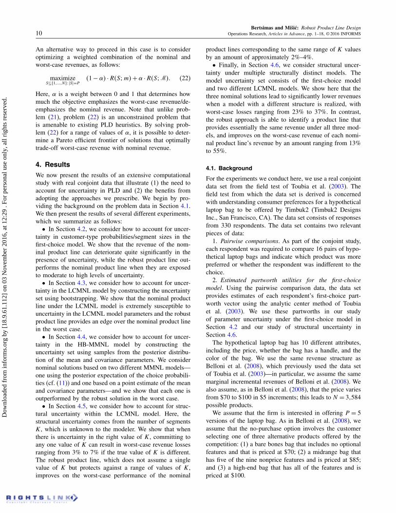
Bertsimas and Mišic: Robust Product Line DesignOperations Research, Articles in Advance, pp. 1–18, © 2016 INFORMS 13

Figure 3. Plot of revenue distributions induced bybootstrapped LCMNL models with K = 2for nominal product line as the number ofrespondents M varies.

40

50

60

70

80

25 50 100 150 200 250 300 330

Num. respondents

Rev

enue

first M respondents in the data set to estimate the LCMNLmodel and find the nominal product line. We then draw B =

100 bootstrap samples, estimate an LCMNL model on eachbootstrap sample, and compute the distribution of revenuesinduced by this bootstrapped collection of models for thenominal product line. Figure 3 plots the revenue distribu-tions obtained from this procedure for values of M rangingfrom 25 to 330 (the full set of respondents). From this plot,we can see that at low sample sizes, there is high variabil-ity in the revenues; at higher sample sizes, this variabilityis greatly reduced. This suggests that robustness is particu-larly valuable in settings where the number of respondentsis low, and becomes a less salient issue when one has alarge number of respondents.

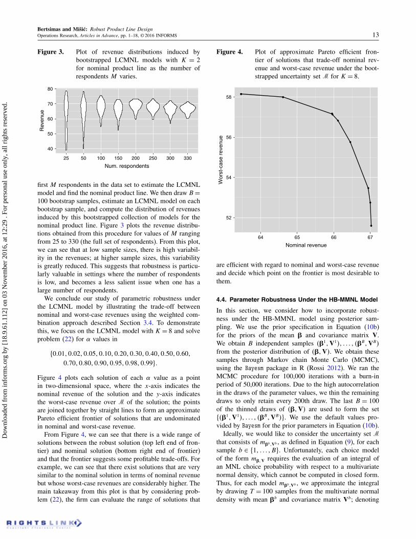
We conclude our study of parametric robustness underthe LCMNL model by illustrating the trade-off betweennominal and worst-case revenues using the weighted com-bination approach described Section 3.4. To demonstratethis, we focus on the LCMNL model with K = 8 and solveproblem (22) for � values in

80001100021000510010100201003010040100501006010070100801009010095100981009990

Figure 4 plots each solution of each � value as a pointin two-dimensional space, where the x-axis indicates thenominal revenue of the solution and the y-axis indicatesthe worst-case revenue over M of the solution; the pointsare joined together by straight lines to form an approximatePareto efficient frontier of solutions that are undominatedin nominal and worst-case revenue.

From Figure 4, we can see that there is a wide range ofsolutions between the robust solution (top left end of fron-tier) and nominal solution (bottom right end of frontier)and that the frontier suggests some profitable trade-offs. Forexample, we can see that there exist solutions that are verysimilar to the nominal solution in terms of nominal revenuebut whose worst-case revenues are considerably higher. Themain takeaway from this plot is that by considering prob-lem (22), the firm can evaluate the range of solutions that

Figure 4. Plot of approximate Pareto efficient fron-tier of solutions that trade-off nominal rev-enue and worst-case revenue under the boot-strapped uncertainty set M for K = 8.

52

54

56

58

64 65 66 67

Nominal revenue

Wor

st-c

ase

reve

nue

are efficient with regard to nominal and worst-case revenueand decide which point on the frontier is most desirable tothem.

4.4. Parameter Robustness Under the HB-MMNL Model

In this section, we consider how to incorporate robust-ness under the HB-MMNL model using posterior sam-pling. We use the prior specification in Equation (10b)for the priors of the mean  and covariance matrix V.We obtain B independent samples 4Â11V151 0 0 0 1 4ÂB1VB5from the posterior distribution of 4Â1V5. We obtain thesesamples through Markov chain Monte Carlo (MCMC),using the Bayesm package in R (Rossi 2012). We ran theMCMC procedure for 100,000 iterations with a burn-inperiod of 50,000 iterations. Due to the high autocorrelationin the draws of the parameter values, we thin the remainingdraws to only retain every 200th draw. The last B = 100of the thinned draws of 4Â1V5 are used to form the set84Â11V151 0 0 0 1 4ÂB1VB59. We use the default values pro-vided by Bayesm for the prior parameters in Equation (10b).

Ideally, we would like to consider the uncertainty set Mthat consists of mÂb1Vb , as defined in Equation (9), for eachsample b ∈ 811 0 0 0 1B9. Unfortunately, each choice modelof the form mÂ1V requires the evaluation of an integral ofan MNL choice probability with respect to a multivariatenormal density, which cannot be computed in closed form.Thus, for each model mÂb1Vb , we approximate the integralby drawing T = 100 samples from the multivariate normaldensity with mean Âb and covariance matrix Vb; denoting

Dow

nloa

ded

from

info

rms.

org

by [

18.9

.61.

112]

on

03 N

ovem

ber

2016

, at 1

2:29

. Fo

r pe

rson

al u

se o

nly,

all

righ

ts r

eser

ved.

Bertsimas and Mišic: Robust Product Line Design14 Operations Research, Articles in Advance, pp. 1–18, © 2016 INFORMS

the approximate choice model by mÂb1Vb , the choice prob-ability of an option p given the product line S is then just

mÂb1Vb4p � S5=

T∑

t=1

1T

exp4ub1 t4p55∑

p′∈S exp4ub1 t4p′55+ exp4ub1 t40551

(27)where ub1 t4 · 5 is the utility function corresponding to thetth sample of the partworth vector u from the multivari-ate normal distribution corresponding to the bth posteriorsample. Our final uncertainty set is thus

M= 8mÂ11V11 0 0 0 1 mÂB1VB90 (28)

We consider two types of nominal models. The first isthe approximate posterior expectation (PostExp) MMNLchoice model, which is defined as

mPostExp4p � S5

=1B

·

B∑

b=1

mÂb1Vb4p � S5

=1BT

B∑

b=1

T∑

t=1

exp4ub1 t4p55∑

p′∈S exp4ub1 t4p′55+ exp4ub1 t40550 (29)

The choice probabilities produced by mPostExp can be viewedas approximations of the true posterior expected choiceprobabilities given in Equation (11). There are two levelsof approximation: the integral over the posterior density of and V is approximated by the average of B samples fromthat posterior density, while the inner integral for each pos-terior sample is approximated by the average of T samplesfrom the corresponding multivariate normal distribution.

The second nominal model we will consider is theapproximate point estimate (PointEst) MMNL choicemodel. Here, we obtain the approximate posterior meanof the mean parameter Â, given by Â∗ = 41/B5 ·

∑Bb=1 Â

b,and the covariance matrix, given by V∗ = 41/B5 ·

∑Bb=1 Vb.

We then plug these point estimates into the definition ofthe MMNL model in Equation (9). Since the integral thatdefines Equation (9) cannot be computed in closed form,we approximate the integral with T = 100 samples from thecorresponding multivariate normal density. Letting u∗1 t4 · 5denote the utility function corresponding to the tth sam-ple from the multivariate normal density with mean Â∗ andcovariance matrix V∗, we define the approximate point esti-mate MMNL choice model as

mPointEst4p � S5=1T

T∑

t=1

exp4u∗1 t4p55∑

p′∈S exp4u∗1 t4p′55+ exp4u∗1 t40550

(30)This approach of replacing the posterior distribution over Âand V by a point estimate is sometimes referred to as the“plug-in” Bayes approach (see Rossi and Allenby 2003).

We optimize each of the resulting objective functions,R4·3M5, R4·3mPostExp5, and R4·3mPointEst5, to obtain theproduct lines SR, SN1mPostExp , and SN1mPointEst , respectively. Foreach nominal solution, we compute the WCL and the RIof the robust solution under the uncertainty set M.

Table 3. Comparison of solutions under nominal HBmodels mPointEst and mPostExp to robust solutionunder uncertainty set M formed by posteriorsampling.

Model m R4SN1m3m5 ($) R4SN1m3M5 ($) WCL (%) RI (%)

mPointEst 61.33 54.88 10.52 6.25mPostExp 62.44 56.89 8.89 2.50

Table 3 shows the nominal and worst-case revenue underM of the nominal product line under each of the two nom-inal HB models, as well as the WCL and RI for eachnominal product line. The worst-case revenue of the robustproduct line is $58.31. From this table, we can see that thenominal product lines obtained using the PostExp modelmPostExp and the PointEst model mPointEst are highly suscep-tible to uncertainty as represented by the uncertainty set M,which is informed by the posterior distribution of the part-worth mean vector  and the covariance matrix V. At thesame time, the robust solution is able to improve the worst-case revenue under M significantly in each case (more than6% for the PointEst model and by 2.5% for the PostExpmodel).

4.5. Structural Robustness Under DifferentLCMNL Models

One of the difficulties of using the LCMNL model in prac-tice is that we do not know a priori what the right numberof customer segments K is. To find the number of seg-ments, one typically estimates the LCMNL model for arange of values of K and then selects the “best” model fromthis set of models. What is meant by “best” is usually amodel that strikes a good balance between fit (as measuredby the log likelihood) and complexity (as measured bythe number of parameters). While there exist metrics suchas the Akaike information criterion (AIC) (Akaike 1974),the Bayesian information criterion (Schwarz 1978), or theconsistent Akaike information criterion (CAIC) (Bozdogan1987) that one can use to quantify the quality of a modeland to guide the selection of a best model (e.g., selectthe model with the best AIC value), these metrics are notinfallible and can often lead to different choices of a bestmodel. In the end, one may only be able to delineate a setof “good” models as opposed to a single “best” model.

To illustrate this with the conjoint data set of Toubia et al.(2003), we estimate the LCMNL model using the pairwisecomparison data for different values of K in 81121 0 0 0 1209.Figures 5 and 6 display the AIC and CAIC, respectively,against the number of customer segments K. From Fig-ure 6, we can see that the CAIC implies a choice of K ofeither 3 or 4. (The minimum CAIC is 6,103.17 at K = 3;the second lowest is 6,104.89 for K = 4.) In contrast, fromFigure 5, we can see that AIC continues decreasing as Kincreases beyond K = 3 until it begins to settle down, start-ing at approximately K = 12. Thus, based on the AIC,

Dow

nloa

ded

from

info

rms.

org

by [

18.9

.61.

112]

on

03 N

ovem

ber

2016

, at 1

2:29

. Fo

r pe

rson

al u

se o

nly,

all

righ

ts r

eser

ved.

Bertsimas and Mišic: Robust Product Line DesignOperations Research, Articles in Advance, pp. 1–18, © 2016 INFORMS 15

Figure 5. AIC for K ∈ 811 0 0 0 1209.

5,500

5,700

5,900

6,100

6,300

2 4 6 8 10 12 14 16 18 20

K

AIC

it would seem that K = 12 would be a more appropriatechoice. Based on these plots, we could conclude that anyvalue of K between 3 and 12 is a reasonable value to select.

We now demonstrate how robustness can be used tocounteract our uncertainty in the number of segments inthe LCMNL model. Given the plots of the AIC and CAICin Figures 5 and 6, we may decide that the number of seg-ments K should lie in the range between 3 and 12. Thus,letting mLCK denote the fitted LCMNL model with K cus-tomer segments, we would define our uncertainty set to be

M= 8mLC31mLC41 0 0 0 1mLC1290 (31)

We would then solve the robust problem (13) with Mto obtain a robust product SR. To compare this solutionagainst the nominal approach, we solve the nominal prob-lem (2) for each mLCK ∈M to obtain a product line SN1K foreach K ∈ 831 0 0 0 1129, and evaluate the worst-case revenueR4SN1K3M5 for each such product line.

Table 4 provides the results of this comparison. The sec-ond column indicates each nominal product line’s nominalrevenue. The third column indicates each nominal productline’s worst-case revenue over M. The fourth column dis-plays the WCL of each nominal product line, while the

Figure 6. CAIC for K ∈ 811 0 0 0 1209.

6,250

6,500

6,750

7,000

CA

IC

2 4 6 8 10 12 14 16 18 20

K

Table 4. Comparison of nominal and worst-case rev-enues of product lines SN131 0 0 0 1 SN112.

No. R4SN1K3mLCK5 R4SN1K3M5 WCL RI

segments K ($) ($) (%) (%)

K = 3 65.34 61.32 6.17 4.15K = 4 64.87 61.56 5.10 3.74K = 5 64.90 61.35 5.47 4.09K = 6 66.19 62.58 5.46 2.05K = 7 64.87 62.71 3.33 1.83K = 8 67.02 62.33 7.01 2.46K = 9 65.14 62.24 4.45 2.60K = 10 65.49 62.33 4.82 2.46K = 11 66.16 62.48 5.57 2.22K = 12 65.80 61.59 6.41 3.69

fifth column displays the RI of the robust product line overeach nominal product line with respect to the worst-caserevenue. The worst-case revenue R4SR3M5 of the robustsolution SR is $63.86.

From this table, we can see that the nominal productlines corresponding to mLC31 0 0 0 1mLC12 are quite suscepti-ble to uncertainty. This is visible from the values of theWCL; the WCL ranges from 3.33% (K = 75 to as muchas 7.01% (K = 8). At the same time, the robust solutionSR provides significant improvement over all of these nom-inal solutions in the worst case. In particular, for the twomodels mLC3 and mLC12 suggested by the CAIC and AICmetrics, respectively, the RIs are 4.15% and 3.69%.

The main takeaway from this analysis is that robust opti-mization provides an alternative to model selection. Whenthe data set does not clearly imply one single “best” model,but instead implies multiple “reasonably good” models,robustness provides a means of simultaneously optimiz-ing against all of these models, rather than optimizing onlyagainst a single one.

4.6. Structural Robustness Under Distinct Models

In Section 4.5, we considered how robust optimization canbe used to account for uncertainty in the number of seg-ments in the LCMNL model. In this section, we take thisidea a step further by using robust optimization to accountfor our uncertainty over structurally distinct models. In par-ticular, in a given application, we may develop models thatmake very different assumptions. For example, we mayestimate a first-choice model, as in Section 4.2, and anLCMNL model as in Sections 4.3 and 4.5. As in Sec-tion 4.5, one model may not clearly stand out as the bestmodel. At the same time, if we make a product line decisionbased on one of these models, the revenue that is garneredmay be significantly lower than anticipated if the marketresponds according to one of the other models.

To demonstrate the value of robustness, we proceed asfollows. We assume that after analyzing the conjoint dataset, we identify the following set of models:

M= 8mFC1mLC31mLC1291 (32)

Dow

nloa

ded

from

info

rms.

org

by [

18.9

.61.

112]

on

03 N

ovem

ber

2016

, at 1

2:29

. Fo

r pe

rson

al u

se o

nly,

all

righ

ts r

eser

ved.

Bertsimas and Mišic: Robust Product Line Design16 Operations Research, Articles in Advance, pp. 1–18, © 2016 INFORMS

Table 5. Performance of nominal and robust product lines under the different models in M,as well as the worst-case model.

Nominal revenue ($)Worst-case revenue ($)

Product line R4·3mFC5 R4·3mLC35 R4·3mLC125 R4·3M5 WCL (%) RI (%)

SN1mFC 72.82 55.74 56.39 55.74 23.45 13.70SN1mLC3 40.98 65.34 61.32 40.98 37.28 54.64SN1mLC12 48.49 62.93 65.80 48.49 26.31 30.69SR 63.69 63.43 63.38 63.38 — —

where mFC is the nominal first-choice model from Sec-tion 4.2 constructed using the estimated partworth vectorsof all 330 respondents and mLC3 and mLC12 are the LCMNLmodels with K = 3 and K = 12 segments, respectively, esti-mated from the pairwise comparison data. For each modelm ∈ M, we solve the nominal PLD problem (2) to obtainthe nominal product line SN1m. We compute the revenueof SN1m under each model m′ ∈ M, as well as its worst-case revenue over M. Then, we solve the robust PLD prob-lem (13) to obtain the robust product line SR, and computethe revenue of SR under each model m′ ∈M, as well as itsworst-case revenue. We compute the WCL of each modelm and the RI of the robust product line SR over the nominalproduct line for each model m.

Table 5 displays the nominal and worst-case revenuesof each of the product lines. From this table, we can seethat committing to a single model leads to significantlylower revenues under the other models. For example, if weassume the first-choice model mFC , the nominal revenue is$72.82, but this reduces to $55.74 if the true model is theK = 3 segment LCMNL model, representing a loss of morethan 20%. If we instead assume the K = 3 LCMNL model,the nominal revenue is $65.34, but this reduces to $40.98if the realized model is the first-choice model (a loss ofmore than 35%). The WCL of all three nominal productlines is more than 20%, indicating that in the worst case,the revenue of each of these product lines deteriorates bymore than 20%.

In contrast to the nominal solution, the robust solutionis able to achieve better worst-case performance, rangingfrom a 13.70% improvement (over the first-choice solu-tion) to 54.64% (over the mLC3 solution). Moreover, therevenue of the robust solution is strikingly consistent overall three models, ranging from $63.38 to $63.69. Althoughthe robust solution is not able to simultaneously achieve thebest performance that is possible for each of the three mod-els, it is able to achieve good performance for all threemodels and achieves better aggregate performance than thesolution of each individual model. In this way, robust opti-mization allows us to incorporate all of the models that wedeem acceptable, rather than just one.

It is also interesting to examine the product lines them-selves. Figures 7–9 display the nominal product lines formFC, mLC3, and mLC12, respectively, while Figure 10 dis-plays the robust product line. The first column indicates

the attribute and each subsequent column represents oneof the products; in a given column, a shaded cell indicatesthat the product has the corresponding attribute. For exam-ple, the fourth product in the first-choice product line ispriced at $100, and has a handle, a PDA holder, a cell-phone holder, and a mesh pocket. For easier comparison,Figure 11 shows the competitive offerings; that is, the prod-ucts comprising the no-purchase option in the same format.

From these figures, we can see that the three nominalproduct lines are very different in terms of the actual prod-ucts. For example, the first-choice product line is structuredin a way that it includes products that directly compete withthe competitive offerings that comprise the no-purchaseoption. As a specific example, consider the third product,which is identical to the high-end bag (see Figure 11) interms of the nonprice features, but is priced at $95 instead

Figure 7. First-choice product line, SN1mFC .

Price $100 $80 $95 $100 $70

Large size

Red color

Logo

Handle

PDA holder

Cellphone holder

Mesh pocket

Velcro flap

Boot

Figure 8. LCMNL model with K = 3 product line,SN1mLC3 .

Price $100 $100 $100 $100 $100

Large size

Red color

Logo

Handle

PDA holder

Cellphone holder

Mesh pocket

Velcro flap

Boot

Dow

nloa

ded

from

info

rms.

org

by [

18.9

.61.

112]

on

03 N

ovem

ber

2016

, at 1

2:29

. Fo

r pe

rson

al u

se o

nly,

all

righ

ts r

eser

ved.

Bertsimas and Mišic: Robust Product Line DesignOperations Research, Articles in Advance, pp. 1–18, © 2016 INFORMS 17

Figure 9. LCMNL model with K = 12 product line,SN1mLC12 .

Price $100 $100 $100 $80 $100

Large size

Red color

Logo

Handle

PDA holder

Cellphone holder

Mesh pocket

Velcro flap

Boot

of $100 and is thus more attractive. In contrast to the first-choice product line, the LCMNL product lines have prod-ucts that are different in terms of features and, in general,are priced higher. This difference in the product lines underthe three models manifests itself in the results of Table 5,which shows how each nominal product line is suboptimalunder one of the other two nominal models.

Comparing the nominal product lines to the robust prod-uct line in Figure 10, we can see that the robust product linecontains three products found in the nominal single-modelproduct lines. Specifically, the third product in the first-choice is identical to the third product in the robust productline; the second product in the LCMNL K = 3 product lineand the fourth product in the robust product line are iden-tical; and the third product in the LCMNL K = 3 productline and the fifth product in the robust product line areidentical. Furthermore, the first and second products of therobust product line differ by one attribute from the third andfirst products, respectively, of the LCMNL K = 12 prod-uct line. Thus the robust product line could be viewed aseffectively “blending” the three single-model product lines.This characteristic of the robust product line agrees withour intuition: by using products that are identical or verysimilar to products in the individual single-model productlines, it seems reasonable to expect that the robust prod-uct line should achieve good performance over all threemodels.

Figure 10. Robust product line, SR.

Price $100 $100 $95 $100 $100

Large size

Red color

Logo

Handle

PDA holder

Cellphone holder

Mesh pocket

Velcro flap

Boot

Figure 11. Competitive products.

Price $70 $85 $100

Large size

Red color

Logo

Handle

PDA holder

Cellphone holder

Mesh pocket

Velcro flap

Boot

5. ConclusionIn this paper, we have extended the familiar nominal PLDproblem to account for parameter uncertainty and structuraluncertainty by adopting a robust optimization approach.With regard to parameter uncertainty, we showed througha number of numerical experiments using a real conjointdata set that parameter uncertainty under three differentwidely used models has the potential to greatly reduce real-ized revenues. We further showed how, using the approachwe have proposed, it is possible to guard against uncer-tainty and to limit its impact on revenues. With regard tostructural uncertainty, we demonstrated that different modelstructures can lead to significantly different product linedecisions, and that each such product line decision maybe highly suboptimal for a different model structure. Wethen showed how optimizing against the worst-case rev-enue over all of the structurally different models leads toproduct lines that achieve good performance over all of themodels and improve on each single-model product line inthe worst case.

A number of possibilities exist for further exploringthe methodology presented here. Apart from the choicemodel, there exist many other sources of uncertainty. Onesuch source of uncertainty is in the cost information; wemay not precisely know the incremental marginal costof each attribute. Another source of uncertainty is in theno-purchase behavior. In particular, we may not preciselyknow the competitive offerings that give rise to the no-purchase option; moreover, these competitive offerings maybe decided in response to the product line that we offer.One could adapt the worst-case framework that we havedescribed here to accommodate these considerations bypopulating the uncertainty set with models that correspondto different competitive response scenarios.

Acknowledgments

The authors thank the area editor Harikesh Nair, the former areaeditor Duncan Simester, the associate editor, and the two anony-mous referees for their helpful and insightful comments thatgreatly improved the paper. The authors gratefully acknowledgethe authors of Toubia et al. (2003) for graciously making theirdata set available, which was used in Section 4. The work of the

Dow

nloa

ded

from

info

rms.

org

by [

18.9

.61.

112]

on

03 N

ovem

ber

2016

, at 1

2:29

. Fo

r pe

rson

al u

se o

nly,

all

righ

ts r

eser

ved.

Bertsimas and Mišic: Robust Product Line Design18 Operations Research, Articles in Advance, pp. 1–18, © 2016 INFORMS

second author was supported by the Natural Sciences and Engi-neering Research Council (NSERC) of Canada through a PGS-Daward.

ReferencesAkaike H (1974) A new look at the statistical model identification. IEEE

Trans. Automatic Control 19(6):716–723.Allenby GM, Rossi PE (1998) Marketing models of consumer heterogene-

ity. J. Econometrics 89(1):57–78.Baron O, Milner J, Naseraldin H (2011) Facility location: A robust opti-

mization approach. Production Oper. Management 20(5):772–785.Belloni A, Freund R, Selove M, Simester D (2008) Optimizing product

line designs: Efficient methods and comparisons. Management Sci.54(9):1544–1552.

Bertsimas D, Sim M (2004) The price of robustness. Oper. Res. 52(1):35–53.

Bertsimas D, Thiele A (2006) A robust optimization approach to inventorytheory. Oper. Res. 54(1):150–168.

Bertsimas D, Brown DB, Caramanis C (2011) Theory and applications ofrobust optimization. SIAM Rev. 53(3):464–501.

Bertsimas D, Silberholz J, Trikalinos T (2016) Optimal healthcare decisionmaking under multiple mathematical models: Application in prostatecancer screening. Health Care Management Sci., ePub ahead of printSeptember 17, https://doi.org/10.1007/s10729-016-9381-3.

Bertsimas D, Litvinov E, Sun XA, Zhao J, Zheng T (2013) Adaptiverobust optimization for the security constrained unit commitmentproblem. IEEE Trans. Power Systems 28(1):52–63.

Besharati B, Luo L, Azarm S, Kannan PK (2006) Multi-objective sin-gle product robust optimization: An integrated design and marketingapproach. J. Mechanical Design 128(4):884–892.

Bezanson J, Karpinski S, Shah VB, Edelman A (2012) Julia:A fast dynamic language for technical computing. Preprint,arXiv:1209.5145.

Bozdogan H (1987) Model selection and Akaike’s information criterion(AIC): The general theory and its analytical extensions. Psychome-trika 52(3):345–370.

Chen KD, Hausman WH (2000) Technical note: Mathematical proper-ties of the optimal product line selection problem using choice-basedconjoint analysis. Management Sci. 46(2):327–332.

Dempster AP, Laird NM, Rubin DB (1977) Maximum likelihood fromincomplete data via the EM algorithm. J. Roy. Statist. Soc. Ser. B39(1):1–38.

Dobson G, Kalish S (1988) Positioning and pricing a product line. Mar-keting Sci. 7(2):107–125.

Dobson G, Kalish S (1993) Heuristics for pricing and positioninga product-line using conjoint and cost data. Management Sci.39(2):160–175.

Goldfarb D, Iyengar G (2003) Robust portfolio selection problems. Math.Oper. Res. 28(1):1–38.

Green PE, Krieger AM (1985) Models and heuristics for product lineselection. Marketing Sci. 4(1):1–19.

Green PE, Krieger AM (1993) Conjoint analysis with product-positioningapplications. Eliashberg J, Lilien GL, eds. Handbooks in OperationsResearch and Management Science, Vol. 5 (Elsevier, Amsterdam),467–515.

Kohli R, Sukumar R (1990) Heuristics for product-line design using con-joint analysis. Management Sci. 36(12):1464–1478.

Kraus UG, Yano CA (2003) Product line selection and pricing under ashare-of-surplus choice model. Eur. J. Oper. Res. 150(3):653–671.

Lubin M, Dunning I (2015) Computing in operations research using Julia.INFORMS J. Comput. 27(2):238–248.

Luo L (2011) Product line design for consumer durables: An inte-grated marketing and engineering approach. J. Marketing Res. 48(1):128–139.

Luo L, Kannan PK, Besharati B, Azarm S (2005) Design of robust newproducts under variability: Marketing meets design. J. Product Inno-vation Management 22(2):177–192.

McBride RD, Zufryden FS (1988) An integer programming approachto the optimal product line selection problem. Marketing Sci. 7(2):126–140.

Rossi PE (2012) Bayesm: Bayesian Inference for Marketing/Micro-econometrics. http://CRAN.R-project.org/package=bayesm. R pack-age version 2.2-5.

Rossi PE, Allenby GM (2003) Bayesian statistics and marketing. Market-ing Sci. 22(3):304–328.

Rossi PE, Allenby GM, McCulloch R (2012) Bayesian Statistics and Mar-keting (John Wiley & Sons, Hoboken, NJ).

Rusmevichientong P, Topaloglu H (2012) Robust assortment optimizationin revenue management under the multinomial logit choice model.Oper. Res. 60(4):865–882.

Sawtooth Software (2003) Advanced Simulation Module (ASM) for Prod-uct Optimization v1.5. Sawtooth Software Technical Paper Series.http://www.sawtoothsoftware.com/download/techpap/asmtech.pdf.

Schön C (2010a) On the optimal product line selection problem with pricediscrimination. Management Sci. 56(5):896–902.

Schön C (2010b) On the product line selection problem under attrac-tion choice models of consumer behavior. Eur. J. Oper. Res. 206(1):260–264.

Schwarz G (1978) Estimating the dimension of a model. Ann. Statist.6(2):461–464.

Toubia O, Simester DI, Hauser JR, Dahan E (2003) Fast polyhedral adap-tive conjoint estimation. Marketing Sci. 22(3):273–303.

Train KE (2008) EM algorithms for nonparametric estimation of mixingdistributions. J. Choice Model. 1(1):40–69.

Train KE (2009) Discrete Choice Methods with Simulation. (CambridgeUniversity Press, New York).

Zufryden FS (1982) Product line optimization by integer programming.Proc. Annual Meeting of ORSA/TIMS, San Diego, CA, 100–114.

Dimitris Bertsimas is the Boeing Professor of OperationsResearch and codirector of the Operations Research Center atthe Massachusetts Institute of Technology. His interests includeanalytics, optimization, and stochastics. This paper is part of hislong-term interest in optimization under uncertainty.

Velibor V. Mišic is an assistant professor of Decisions, Oper-ations, and Technology Management at the Anderson School ofManagement, University of California, Los Angeles. His researchinterests are in analytics, operations management, marketing sci-ence, and optimization under uncertainty, the latter two of whichthis paper is a part.

Dow

nloa

ded

from

info

rms.

org

by [

18.9

.61.

112]

on

03 N

ovem

ber

2016

, at 1

2:29

. Fo

r pe

rson

al u

se o

nly,

all

righ

ts r

eser

ved.