Embed Size (px)
Citation preview
Robust Sensitivity Analysis of theOptimal Value of Linear Programming
Guanglin Xu∗ Samuel Burer†
September 14, 2015Revised: November 4, 2015
AbstractWe propose a framework for sensitivity analysis of linear programs (LPs) in minimiza-tion form, allowing for simultaneous perturbations in the objective coefficients andright-hand sides, where the perturbations are modeled in a compact, convex uncer-tainty set. This framework unifies and extends multiple approaches for LP sensitiv-ity analysis in the literature and has close ties to worst-case linear optimization andtwo-stage adaptive optimization. We define the minimum (best-case) and maximum(worst-case) LP optimal values, p− and p+, over the uncertainty set, and we discussissues of finiteness, attainability, and computational complexity. While p− and p+ aredifficult to compute in general, we prove that they equal the optimal values of twoseparate, but related, copositive programs. We then develop tight, tractable conicrelaxations to provide lower and upper bounds on p− and p+, respectively. We alsodevelop techniques to assess the quality of the bounds, and we validate our approachcomputationally on several examples from—and inspired by—the literature. We findthat the bounds on p− and p+ are very strong in practice and, in particular, are atleast as strong as known results for specific cases from the literature.
Keywords: Sensitivity analysis, minimax problem, nonconvex quadratic programming,semidefinite programming, copositive programming, uncertainty set.
1 Introduction
The standard-form linear program (LP) is
min cTx
s. t. Ax = b
x ≥ 0
(1)
∗Department of Management Sciences, University of Iowa, Iowa City, IA, 52242-1994, USA. Email:[email protected].†Department of Management Sciences, University of Iowa, Iowa City, IA, 52242-1994, USA. Email:
1
arX
iv:1
509.
0468
2v2
[m
ath.
OC
] 7
Nov
201
5
where x ∈ Rn is the variable and (A, b, c) ∈ Rm×n × Rm × Rn are the problem parameters.
In practice, (A, b, c) may not be known exactly or may be predicted to change within a
certain region. In such cases, sensitivity analysis (SA) examines how perturbations in the
parameters affect the optimal value and solution of (1). Ordinary SA considers the change of
a single element in (A, b, c) and examines the corresponding effects on the optimal basis and
tableau; see [8]. SA also extends to the addition of a new variable or constraint, although
we do not consider such changes in this paper.
Beyond ordinary SA, more sophisticated approaches that allow simultaneous changes in
the coefficients c or right-hand sides b have been proposed by numerous researchers. Bradley
et al. [4] discuss the 100-percent rule that requires specification of directions of increase or
decrease from each cj and then guarantees that the same basis remains optimal as long as
the sum of fractions, corresponding to the percent of maximum change in each direction
derived from ordinary SA, is less than or equal to 1. Wendell [35, 36, 37] develops the
tolerance approach to find the so-called maximum tolerance percentage by which the objective
coefficients can be simultaneously and independently perturbed within a priori bounds. The
tolerance approach also handles perturbations in one row or column of the matrix coefficients
[31] or even more general perturbations in all elements of the matrix coefficients under certain
assumptions [30]. Freund [15] investigates the sensitivity of an LP to simultaneous changes
in matrix coefficients. In particular, he considers a linear program whose coefficient matrix
depends linearly on a scalar parameter θ and studies the effect of small perturbations on the
the optimal objective value and solution; see also [21, 22, 28]. Readers are referred to [34]
for a survey of approaches for SA of problem (1).
An area closely related to SA is interval linear programming (ILP), which can be viewed as
multi-parametric linear programming with independent interval domains for the parameters
[17, 18, 26]. Steuer [33] presents three algorithms for solving LPs in which the objective
coefficients are specified by intervals, and Gabrel et al. [16] study LPs in which the right-
hand sides vary within intervals and discuss the maximum and minimum optimal values.
Mraz [27] considers a general situation in which the matrix coefficients and right-hand sides
change within intervals and calculates upper and lower bounds for the associated optimal
values. A comprehensive survey of ILP has been given by Hladik [20].
To the best of our knowledge, in the context of LP, no authors have considered simulta-
neous LP parameter changes in a general way, i.e., perturbations in the objective coefficients
c, right-hand sides b, and constraint coefficients A within a general region (not just inter-
vals). The obstacle for doing so is clear: general perturbations lead to nonconvex quadratic
programs (QPs), which are NP-hard to solve (as discussed below).
In this paper, we extend—and in many cases unify—the SA literature by employing
2
modern tools for nonconvex QPs. Specifically, we investigate SA for LPs in which (b, c)
may change within a general compact, convex set U , called the uncertainty set . Our goal
is to calculate—or bound—the corresponding minimum (best-case) and maximum (worst-
case) optimal values. Since these values involve the solution of nonconvex QPs, we use
standard techniques from copositive optimization to reformulate these problems into convex
copositive programs (COPs), which provide a theoretical grounding upon which to develop
tight, tractable convex relaxations. We suggest the use of semidefinite programming (SDP)
relaxations, which also incorporate valid conic inequalities that exploit the structure of the
uncertainty set. We refer the reader to [10] for a survey on copositive optimization and
its connections to semidefinite programming. Relevant definitions and concepts will also be
given in this paper; see Section 1.1.
Our approach is related to the recent work on worst-case linear optimization introduced
by Peng and Zhu [29] in which: (i) only b is allowed to change within an ellipsoidal region; and
(ii) only the worst-case LP value is considered. (In fact, one can see easily that, in the setup
of [29] based on (i), the best-case LP value can be computed in polynomial time via second-
order-cone programming, making it less interesting to study in their setup.) The authors
argue that the worst-case value is NP-hard to compute and use a specialized nonlinear
semidefinite program (SDP) to bound it from above. They also develop feasible solutions to
bound the worst-case value from below and show through a series of empirical examples that
the resulting gaps are usually quite small. Furthermore, they also demonstrate that their
SDP-based relaxation is better than the so-called affine-rule approximation (see [2]) and the
Lasserre linear matrix inequality relaxation (see [24, 19]).
Our approach is more general than [29] because we allow both b and c to change, we
consider more general uncertainty sets, and we study both the worst- and best-case values.
In addition, instead of developing a specialized SDP approach, we make use of the machinery
of copositive programming, which provides a theoretical grounding for the construction of
tight, tractable conic relaxations using existing techniques. Nevertheless, we have been
inspired by their approach in several ways. For example, their proof of NP-hardness also
shows that our problem is NP-hard; we will borrow their idea of using primal solutions to
estimate the quality of the relaxation bounds; and we test some of the same examples.
We mention two additional connections of our approach with the literature. In [3],
Bertsimas and Goyal consider a two-stage adaptive linear optimization problem under right-
hand side uncertainty with a min-max objective. A simplified version of this problem, in
which the first-stage variables are non-existent, reduces to worst-case linear optimization;
see the introduction of [3]. In fact, Bertsimas and Goyal use this fact to prove that their
problem is NP-hard via the so-called max-min fractional set cover problem, which is a specific
3
worst-case linear optimization problem studied by Feige et al. [14]. Our work is also related
to the study of adjustable robust optimization [2, 39], which allows for two sets of decisions—
one that must be made before the uncertain data is realized, and one after. In fact, our
problem can viewed as a simplified case of adjustable robust optimization having no first-
stage decisions. On the other hand, our paper is distinguished by its application to sensitivity
analysis and its use of copositive and semidefinite optimization.
We organize the paper as follows. In Section 2, we extend many of the existing approaches
for SA by considering simultaneous, general changes in (b, c) and the corresponding effect
on the LP optimal value. Precisely, we model general perturbations of (b, c) within a com-
pact, convex set U—the uncertainty set, borrowing terminology from the robust-optimization
literature—and define the corresponding minimum and maximum optimal values p− and p+,
respectively. We call our approach robust sensitivity analysis , or RSA. Then, continuing in
Section 2, we formulate the calculation of p− and p+ as nonconvex bilinear QPs (or BQPs)
and briefly discuss attainability and complexity issues. We also discuss how p− and p+ may
be infinite and suggest alternative bounded variants, q− and q+, which have the property
that, if p− is already finite, then q− = p− and similarly for q+ and p+. Compared to re-
lated approaches in the literature, our discussion of finiteness is unique. We then discuss the
addition of redundant constraints to the formulations of q− and q+, which will strengthen
later relaxations. Section 3 then establishes COP reformulations of the nonconvex BQPs by
directly applying existing reformulation techniques. Then, based on the COPs, we develop
tractable SDP-based relaxations that incorporate the structure of the uncertainty set U , and
we also discuss procedures for generating feasible solutions of the BQPs, which can also be
used to verify the quality of the relaxation bounds. In Section 4, we validate our approach on
several examples, which demonstrate that the relaxations provide effective approximations
of q+ and q−. In fact, we find that the relaxations admit no gap with q+ and q− for all tested
examples.
We mention some caveats about the paper. First, we focus only on how the optimal
value is affected by uncertainty, not the optimal solution. We do so because we believe
this will be a more feasible first endeavor; determining how general perturbations affect
the optimal solution can certainly be a task for future research. Second, as mentioned
above, we believe we are the first to consider these types of general perturbations, and thus
the literature with which to compare is somewhat limited. However, we connect with the
literature whenever possible, e.g., in special cases such as interval perturbations and worst-
case linear optimization. Third, since we do not make any distributional assumptions about
the uncertainty of the parameters, nor about their independence or dependence, we believe
our approach aligns well with the general sprit of robust optimization. It is important to
4
note, however, that our interest is not robust optimization and is not directly comparable to
robust optimization. For example, while in robust optimization one wishes to find a single
optimal solution that works well for all realizations of the uncertain parameters, here we are
only concerned with how the optimal value changes as the parameters change. Finally, we
note the existence of other relaxations for nonconvex QPs including LP relaxations (see [32])
and Lasserre-type SDP relaxations. Generally speaking, LP-based relaxations are relatively
weak (see [1]); we do not consider them in this paper. In addition, SDP approaches can often
be tailored to outperform the more general Lasserre approach as has been demonstrated in
[29]. Our copostive- and SDP-based approach is similar; see for example the valid inequalities
discussed in Section 3.2.
1.1 Notation, terminology, and copositive optimization
Let Rn denote n-dimensional Euclidean space represented as column vectors, and let Rn+
denote the nonnegative orthant in Rn. For a scalar p ≥ 1, the p-norm of v ∈ Rn is defined
‖v‖p := (∑n
i=1 |vi|p)1/p, e.g., ‖v‖1 =∑n
i=1 |vi|. We will drop the subscript for the 2-norm,
e.g., ‖v‖ := ‖v‖2. For v, w ∈ Rn, the inner product of v and w is defined as vTw =∑n
i=1 viwi
and the Hadamard product of v and w is defined by v ◦ w := (v1w1, ..., vnwn)T ∈ Rn.
Rm×n denotes the set of real m × n matrices, and the trace inner product of two matrices
A,B ∈ Rm×n is defined A • B := trace(ATB). Sn denotes the space of n × n symmetric
matrices, and for X ∈ Sn, X � 0 denotes that X is positive semidefinite. In addition,
diag(X) denotes the vector containing the diagonal entries of X.
We also make several definitions related to copositive programming . The n×n copositive
cone is defined as
COP(Rn+) := {M ∈ Sn : xTMx ≥ 0 ∀ x ∈ Rn
+},
and its dual cone, the completely positive cone, is
CP(Rn+) := {X ∈ Sn : X =
∑kx
k(xk)T , xk ∈ Rn+},
where the summation over k is finite but its cardinality is unspecified. The term copositive
programming refers to linear optimization over COP(Rn+) or, via duality, linear optimization
over CP(Rn+). A more general notion of copositive programming is based on the following
5
ideas. Let K ⊆ Rn be a closed, convex cone, and define
COP(K) := {M ∈ Sn : xTMx ≥ 0 ∀ x ∈ K},
CP(K) := {X ∈ Sn : X =∑
kxk(xk)T , xk ∈ K}.
Then generalized copositive programming is linear optimization over COP(K) and CP(K)
and is also sometimes called set-semidefinite optimization [11]. In this paper, we work
with generalized copositive programming, although we will use the shorter phrase copositive
programming for convenience.
2 Robust Sensitivity Analysis
In this section, we introduce the concept of robust sensitivity analysis of the optimal value of
the linear program (1). In particular, we define the best-case optimal value p− and the worst-
case optimal value p+ over the uncertainty set U , which contains general perturbations in
the objective coefficients c and the right-hand sides b. We then propose nonconvex bilinear
QPs (BQPs) to compute p− and p+. Next, we clarify when p− and p+ could be infinite
and propose finite, closely related alternatives q+ and q−, which can also be formulated
as nonconvex BQPs. Importantly, we prove that q− equals p− whenever p− is finite; the
analogous relationship is also proved for q+ and p+.
2.1 The best- and worst-case optimal values
In the Introduction, we have described b and c as parameters that could vary, a concept
that we now formalize. Hereafter, (b, c) denotes the nominal , “best guess” parameter values,
and we let (b, c) denote perturbations with respect to (b, c). In other words, the true data
could be (b + b, c + c), and we think of b and c as varying. We also denote the uncertainty
set containing all possible perturbations (b, c) as U ⊆ Rm × Rn. Throughout this paper, we
assume the following:
Assumption 1. U is compact and convex, and U contains (0, 0).
Given (b, c) ∈ U , we define the perturbed optimal value function at (b, c) as
p(b, c) := min{(c+ c)Tx : Ax = b+ b, x ≥ 0}. (2)
For example, p(0, 0) is the nominal optimal value of the nominal problem based on the nomi-
nal parameters. The main idea of robust sensitivity analysis is then to compute the infimum
6
(best-case) and supremum (worst-case) of all optimal values p(b, c) over the uncertainty set
U , i.e., to calculate
p− := inf{p(b, c) : (b, c) ∈ U}, (3)
p+ := sup{p(b, c) : (b, c) ∈ U}. (4)
We illustrate p− and p+ with a small example.
Example 1. Consider the nominal LP
min x1 + x2
s. t. x1 + x2 = 2
x1, x2 ≥ 0
(5)
and the uncertainty set
U :=
{(b, c) :
b1 ∈ [−1, 1]
c1 ∈ [−0.5, 0.5], c2 = 0
}.
Note that the perturbed data b1 + b1 and c1 + c1 remain positive, while c2 + c2 is constant.
Thus, the minimum optimal value p− occurs when b1 and c1 are minimal, i.e., when b1 = −1
and c1 = −0.5. In this case, p− = 0.5 at the solution (x1, x2) = (1, 0). In a related manner,
p+ = 3 when b1 = 1 and c1 = 0.5 at the point (x1, x2) = (0, 3). Actually, any perturbation
with c1 ∈ [0, 0.5] and b1 = 1 realizes the worst-case value p+ = 3. Figure 1 illustrates this
example.
We can obtain a direct formulation of p− by simply collapsing the inner and outer mini-
mizations of (3) into a single nonconvex BQP:
infb,c,x (c+ c)Tx
s. t. Ax = b+ b, x ≥ 0
(b, c) ∈ U .(6)
The nonconvexity comes from the bilinear term cTx in the objective function. In the special
case that (b, c) ∈ U implies c = 0, i.e., when there is no perturbation in the objective
coefficients, we have the following:
Remark 1. If U is tractable and c = 0 for all (b, c) ∈ U , then p− can be computed in
polynomial time as the optimal value of (6) with c = 0, which is a convex program.
7
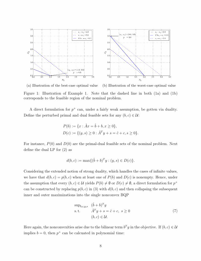
(a) Illustration of the best-case optimal value (b) Illustration of the worst-case optimal value
Figure 1: Illustration of Example 1. Note that the dashed line in both (1a) and (1b)corresponds to the feasible region of the nominal problem.
A direct formulation for p+ can, under a fairly weak assumption, be gotten via duality.
Define the perturbed primal and dual feasible sets for any (b, c) ∈ U :
P (b) := {x : Ax = b+ b, x ≥ 0},
D(c) := {(y, s) ≥ 0 : ATy + s = c+ c, s ≥ 0}.
For instance, P (0) and D(0) are the primal-dual feasible sets of the nominal problem. Next
define the dual LP for (2) as
d(b, c) := max{(b+ b)Ty : (y, s) ∈ D(c)}.
Considering the extended notion of strong duality, which handles the cases of infinite values,
we have that d(b, c) = p(b, c) when at least one of P (b) and D(c) is nonempty. Hence, under
the assumption that every (b, c) ∈ U yields P (b) 6= ∅ or D(c) 6= ∅, a direct formulation for p+
can be constructed by replacing p(b, c) in (3) with d(b, c) and then collapsing the subsequent
inner and outer maximizations into the single nonconvex BQP
supb,c,y,s (b+ b)Ty
s. t. ATy + s = c+ c, s ≥ 0
(b, c) ∈ U .(7)
Here again, the nonconvexities arise due to the bilinear term bTy in the objective. If (b, c) ∈ Uimplies b = 0, then p+ can be calcuated in polynomial time:
8
Remark 2. If U is tractable and b = 0 for all (b, c) ∈ U , then p+ can be computed in
polynomial time as the optimal value of (7) with b = 0, which is a convex program.
We summarize the above discussion in the following proposition:
Proposition 1. The best-case value p− equals the optimal value of (6). Moreover, if P (b) 6= ∅or D(c) 6= ∅ for all (b, c) ∈ U , then the worst-case value p+ equals the optimal value of (7).
We view the condition in Proposition 1—that at least one of P (b) and D(c) is nonempty
for each (b, c) ∈ U—to be rather mild. Said differently, the case that P (b) = D(c) = ∅ for
some (b, c) ∈ U appears somewhat pathological. For practical purposes, we hence consider
(7) to be a valid formulation of p+. Actually, in the next subsection, we will further restrict
our attention to those (b, c) ∈ U for which both P (b) and P (c) are nonempty. In such cases,
each p(b, c) is guaranteed to be finite, which—as we will show—carefully handles the cases
when p+ and p− are infinite.
Indeed, the worst-case value p+ could equal +∞ due to some perturbed P (b) being empty
as shown in the following example:
Example 2. In Example 1, change the uncertainty set to
U :=
{(b, c) :
b1 ∈ [−3, 1]
c1 ∈ [−0.5, 0.5], c2 = 0
}.
Then p(b, c) = +∞ whenever b1 ∈ [−3,−2) since then the primal feasible set P (b) is empty.
Then p+ = +∞ overall. However, limiting b1 to [−2, 1] yields a worst-case value of 3 as
discussed in Example 1.
Similarly, p− might equal −∞ due to some perturbed LP having unbounded objective value,
implying infeasibility of the corresponding dual feasible set D(c).
2.2 Attainability and complexity
In this brief subsection, we mention results pertaining to the attainability of p− and p+ and
the computational complexity of computing them.
By an existing result concerning the attainability of the optimal value of nonconvex
BQPs, we have that p− and p+ are attainable when U has a relatively simple structure:
Proposition 2 (theorem 2 of [25]). Suppose U is representable by a finite number of linear
constraints and at most one convex quadratic constraint. Then, if the optimal value of (6)
is finite, it is attained. A similar statement holds for (7).
9
In particular, attainability holds when U is polyhedral or second-order-cone representable
with at most one second-order cone. Moreover, the bilinear nature of (6) implies that, if the
optimal value is attained, then there exists an optimal solution (x∗, b∗, c∗) with (b∗, c∗) an
extreme point of U . The same holds for (7) if its optimal value is attained.
As discussed in the Introduction, the worst-case value p+ has been studied by Peng and
Zhu [29] for the special case when c = 0 and b is contained in an ellipsoid. The authors
demonstrate (see their proposition 1.1) that calculating p+ in this case is NP-hard. By the
symmetry of duality, it thus also holds that p− is NP-hard to compute in general.
2.3 Finite variants of p− and p+
We now discuss closely related variants of p+ and p− that are guaranteed to be finite and
to equal p+ and p−, respectively, when those values are themselves finite. We require the
following feasibility and boundedness assumption:
Assumption 2. Both feasible sets P (0) and D(0) are nonempty, and one is bounded.
By standard theory, P (0) and D(0) cannot both be nonempty and bounded. Also define
U := {(b, c) ∈ U : P (b) 6= ∅, D(c) 6= ∅}.
Note that (0, 0) ∈ U due to Assumption 2. In fact, U can be captured with linear constraints
that enforce primal-dual feasibility and hence is a compact, convex subset of U :
U =
{(b, c) ∈ U :
Ax = b+ b, x ≥ 0
ATy + s = c+ c, s ≥ 0
}.
Analogous to p+ and p−, define
q+ := sup{p(b, c) : (b, c) ∈ U} (8)
q− := inf{p(b, c) : (b, c) ∈ U}. (9)
The following proposition establishes the finiteness of q+ and q−:
Proposition 3. Under Assumptions 1 and 2, both q+ and q− are finite.
Proof. We prove the contrapositive for q−. (The argument for q+ is similar.) Suppose
q− = −∞. Then there exists a sequence {(bk, ck)} ⊆ U with finite optimal values p(bk, ck)→−∞. By strong duality, there exists a primal-dual solution sequence {(xk, yk, sk)} with
10
(c + c)Txk = (b + b)Tyk → −∞. Since U is bounded, it follows that ‖xk‖ → ∞ and
‖yk‖ → ∞.
Consider the sequence {(zk, dk)} with (zk, dk) := (xk, bk)/‖xk‖. We have Azk = b/‖xk‖+
dk, zk ≥ 0, and ‖zk‖ = 1 for all k. Morover, b/‖xk‖ + dk → 0. Hence, there exists a
subsequence converging to (z, 0) such that Az = 0, z ≥ 0, and ‖z‖ = 1. This proves that
the recession cone of P (0) is nontrivial, and hence P (0) is unbounded. In a similar manner,
D(0) is unbounded, which means Assumption 2 does not hold.
Note that the proof of Proposition 3 only assumes that U , and hence U , is bounded, which
does not use the full power of Assumption 1.
Similar to p−, a direct formulation of q− can be constructed by employing the primal-dual
formulation of U and by collapsing the inner and outer minimizations of (9) into a single
nonconvex BQP:
q− = infb,c,x,y,s (c+ c)Tx
s. t. Ax = b+ b, x ≥ 0
ATy + s = c+ c, s ≥ 0
(b, c) ∈ U .
(10)
Likewise for p+, after replacing p(b, c) in (8) by d(b, c), we can collapse the inner and outer
maximizations into a single nonconvex BQP:
q+ = supb,c,x,y,s (b+ b)Ty
s. t. Ax = b+ b, x ≥ 0
ATy + s = c+ c, s ≥ 0
(b, c) ∈ U .
(11)
The following proposition establishes q+ = p+ when p+ is finite and, similarly, q− = p−
when p− is finite.
Proposition 4. If p+ is finite, then q+ = p+, and if p− is finite, then q− = p−.
Proof. We prove the second statement only since the first is similar. Comparing the formu-
lation (6) for p− and the formulation (10) for q−, it is clear that p− ≤ q−. In addition, let
(b, c, x) be any feasible solution of (6). Because p− is finite, p(b, c) is finite. Then the cor-
responding dual problem is feasible, which implies that we can extend (b, c, x) to a solution
(b, c, x, y, s) of (10) with the same objective value. Hence, p− ≥ q−.
In the remaining sections of the paper, we will focus on the finite variants q− and q+ given
by the nonconvex QPs (10) and (11), which optimize the optimal value function p(b, c) =
11
d(b, c) based on enforcing primal-dual feasibility. It is clear that we may also enforce the
complementary slackness condition x ◦ s = 0 without changing these problems. Although
it might seem counterintuitive to add the redundant, nonconvex constraint x ◦ s = 0 to an
already difficult problem, in Section 3, we will propose convex relaxations to approximate
q− and q+, in which case—as we will demonstrate—the relaxed versions of the redundant
constraint can strengthen the relaxations.
3 Copositve Formulations and Relaxations
In this section, we use copositive optimization techniques to reformulate the RSA problems
(10) and (11) into convex programs. We further relax the copositive programs into conic,
SDP-based problems, which are computationally tractable.
3.1 Copositive formulations
In order to formulate (10) and (11) as COPs, we apply a result of [6]; see also [5, 9, 12].
Consider the general nonconvex QP
inf zTWz + 2wT z (12)
s. t. Ez = f, z ∈ K
where K is a closed, convex cone. Its copositive reformulation is
inf W • Z + 2wT z (13)
s. t. Ez = f, diag(EZET ) = f ◦ f(1 zT
z Z
)∈ CP(R+ ×K),
as established by the following lemma:
Lemma 1 (corollary 8.3 in [6]). Problem (12) is equivalent to (13), i.e.: (i) both share the
same optimal value; (ii) if (z∗, Z∗) is optimal for (13), then z∗ is in the convex hull of optimal
solutions for (12).
The following theorem establishes that problems (10) and (11) can be reformulated as
copositive programs according to Lemma 1. The proof is based on describing how the two
problems fit the form (12).
12
Theorem 1. Problems (10) and (11) to compute q− and q+ are solvable as copositive pro-
grams of the form (13), where
K := hom(U)× Rn+ × Rm × Rn
+
and
hom(U) := {(t, b, c) ∈ R+ × Rm × Rn : t > 0, (b, c)/t ∈ U} ∪ {(0, 0, 0)}
is the homogenization of U .
Proof. We prove the result for just problem (10) since the argument for problem (11) is
similar. First, we identify z ∈ K in (12) with (t, b, c, x, y, s) ∈ hom(U) × Rn+ × Rm × Rn
+ in
(10). In addition, in the constraints, we identify Ez = f with the equations Ax = tb + b,
ATy + s = tc + c, and t = 1. Note that the right-hand-side vector f is all zeros except for
a single entry corresponding to the constraint t = 1. Moreover, in the objective, zTWz is
identified with the bilinear term cTx, and 2wT z is identified with the linear term cTx. With
this setup, it is clear that (10) is an instance of (12) and hence Lemma 1 applies to complete
the proof.
3.2 SDP-based conic relaxations
As discussed above, the copositive formulations of (10) and (11) as represented by (13) are
convex yet generally intractable. Thus, we propose SDP-based conic relaxations that are
polynomial-time solvable and hopefully quite tight in practice. In Section 4 below, we will
investigate their tightness computationally.
We propose relaxations that are formed from (13) by relaxing the cone constraint
M :=
(1 zT
z Z
)∈ CP(R+ ×K).
As is well known—and direct from the definitions—cones of the form CP(·) are contained
in the positive semidefinite cone. Hence, we will enforce M � 0. It is also true that
M ∈ CP(R+ × K) implies z ∈ K, although M � 0 does not necessarily imply this. So, in
our relaxations, we will also enforce z ∈ K. Including z ∈ K improves the relaxation and
also helps in the calculation of bounds in Section 3.3
Next, suppose that the description of R+ × K contains at least two linear constraints,
aT1 z ≤ b1 and aT2 z ≤ b2. By multiplying b1 − aT1 z and b2 − aT2 z, we obtain a valid, yet
redundant, quadratic constraint b1b2 − b1aT2 z − b2aT1 z + aT1 zzTa2 ≥ 0 for CP(R+ ×K). This
quadratic inequality can in turn be linearized in terms of M as b1b2−b1aT2 z−b2aT1 z+aT1Za2 ≥
13
0, which is valid for CP(R+×K). We add this linear inequality to our relaxation; it is called
an RLT constraint [32]. In fact, we add all such RLT constraints arising from all pairs of
linear constraints present in the description of R+ ×K.
When the description of R+ × K contains at least one linear constraint aT1 z ≤ b1 and
one second-order-cone constraint ‖d2 − CT2 z‖ ≤ b2 − aT2 z, where d2 is a vector and C2 is a
matrix, we will add a so-called SOC-RLT constraint to our relaxation [7]. The constraint is
derived by multiplying the two constraints to obtain the valid quadratic second-order-cone
constraint
‖(b1 − aT1 z)(d2 − CT2 z)‖ ≤ (b1 − aT1 z)(b2 − aT2 z).
After linearization by M , we have the second-order-cone constraint
‖b1d2 − d2aT1 z − b1CT2 z + CT
2 Za1‖ ≤ b1b2 − b1aT2 z − b2aT1 z + aT1Za2.
Finally, recall the redundant complementarity constraint x◦s = 0 described at the end of
Section 2.3, which is valid for both (10) and (11). Decomposing it as xisi = 0 for i = 1, . . . , n,
we may translate these n constraints to (13) as zTHiz = 0 for appropriatly defined matrices
matrices Hi. Then they may be linearized and added to our relaxation as Hi • Z = 0.
To summarize, let RLT denote the set of (z, Z) satisfying all the derived RLT constraints,
and similarly, define SOCRLT as the set of (z, Z) satisfying all the derived SOC-RLT con-
straints. Then the SDP-based conic relaxation for (13) that we propose to solve is
inf W • Z + 2wT z
s. t. Ez = f, diag(EZET ) = f ◦ fHi • Z = 0 ∀ i = 1, . . . , n
(z, Z) ∈ RLT∩ SOCRLT(1 zT
z Z
)� 0, z ∈ K.
(14)
It is worth mentioning that, in many cases, the RLT and SOC-RLT constraints will already
imply z ∈ K, but in such cases, we nevertheless write the constraint in (14) for emphasis;
see also Section 3.3 below.
When translated to the problem (10) for calculating q−, the relaxation (14) gives rise to
a lower bound q−sdp ≤ q−. Similarly, when applied to (11), we get an upper bound q+sdp ≥ q+.
14
3.3 Bounds from feasible solutions
In this section, we discuss two methods to approximate q− from above and q+ from below,
i.e., to bound q− and q+ using feasible solutions of (10) and (11), respectively.
The first method, which has been inspired by [29], utilizes the optimal solution of the
SDP relaxation (14). Let us discuss how to obtain such a bound for (10), as the discussion
for (11) is similar. We first observe that any feasible solution (z, Z) of (14) satisfies Ez = f
and z ∈ K, i.e., z satisfies all of the constraints of (12). Since (12) is equivalent to (10)
under the translation discussed in the proof of Theorem 1, z gives rise to a feasible solution
(x, y, s, b, c) of (10). From this feasible solution, we can calculate (c+c)Tx ≥ q−. In practice,
we will start from the optimal solution (z−, Z−) of (14). We summarize this approach in the
following remark.
Remark 3. Suppose that (z−, Z−) is an optimal solution of the relaxation (14) corresponding
to (10), and let (x−, y−, s−, b−, c−) be the translation of z− to a feasible point of (10). Then,
r− := (c + c−)Tx− ≥ q−. Similarly, we define r+ := (b + b+)Ty+ ≤ q+ based on an optimal
solution (z+, Z+) of (14) corresponding to (11).
Our second method for bounding q− and q+ using feasible solutions is a sampling proce-
dure detailed in Algorithm 1. The main idea is to generate randomly a point (b, c) ∈ U and
then to calculate p(b, c), which serves as an upper bound of p− and a lower bound of p+,
i.e., p− ≤ p(b, c) ≤ p+. Multiple points (bk, ck) and values pk := p(bk, ck) are generated and
the best bounds p− ≤ v− := mink{pk} and maxk{pk} =: v+ ≤ p+ are saved. In fact, by the
bilinearity of (10) and (11), we we may restrict attention to the extreme points (b, c) of Uwithout reducing the quality of the resultant bounds; see also the discussion in Section 2.2.
Hence, Algorithm 1 generates—with high probability—a random extreme point of U by op-
timizing a random linear objective over U , and we generate the random linear objective as a
vector uniform on the sphere, which is implemented by a well-known, quick procedure. Note
that, even though the random objective is generated according to a specific distribution, we
cannot predict the resulting distribution over the extreme points of U .
As all four of the bounds r−, r+, v−, and v+ are constructed from feasible solutions, we
can further improve them heuristically by exploiting the bilinear objective functions in (10)
and (11). In particular, we employ the standard local improvement heuristic for programs
with a bilinear objective and convex constraints (e.g., see [23]). Suppose, for example, that
we have a feasible point (x−, y−, s−, b−, c−) for problem (10) as discussed in Remark 3. To
attempt to improve the solution, we fix the variable c in (10) at the value c−, and we solve the
resulting convex problem for a new, hopefully better point (x1, y1, s1, b1, c1), where c1 = c−.
Then, we fix x to x1, resolve, and get a new point (x2, y2, s2, b2, c2), where x2 = x1. This
15
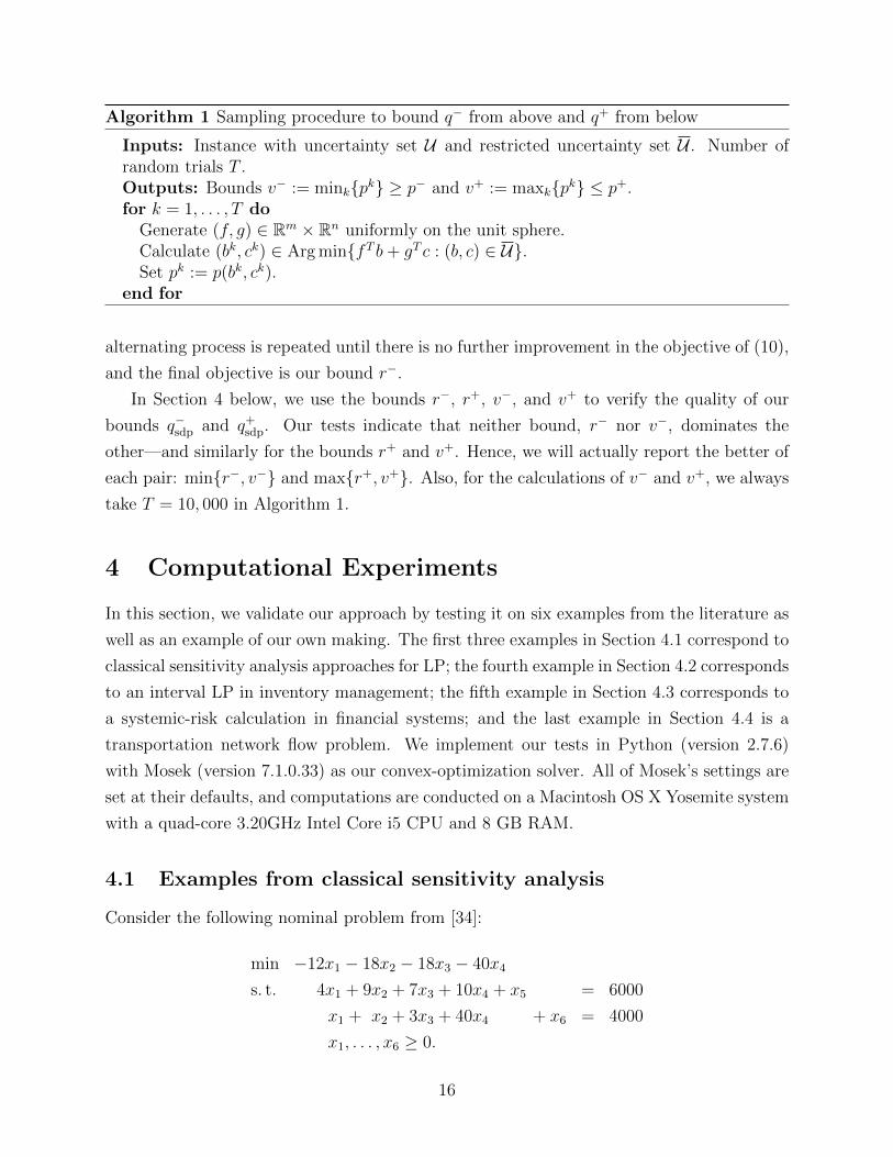
Algorithm 1 Sampling procedure to bound q− from above and q+ from below
Inputs: Instance with uncertainty set U and restricted uncertainty set U . Number ofrandom trials T .Outputs: Bounds v− := mink{pk} ≥ p− and v+ := maxk{pk} ≤ p+.for k = 1, . . . , T do
Generate (f, g) ∈ Rm × Rn uniformly on the unit sphere.Calculate (bk, ck) ∈ Arg min{fT b+ gT c : (b, c) ∈ U}.Set pk := p(bk, ck).
end for
alternating process is repeated until there is no further improvement in the objective of (10),
and the final objective is our bound r−.
In Section 4 below, we use the bounds r−, r+, v−, and v+ to verify the quality of our
bounds q−sdp and q+sdp. Our tests indicate that neither bound, r− nor v−, dominates the
other—and similarly for the bounds r+ and v+. Hence, we will actually report the better of
each pair: min{r−, v−} and max{r+, v+}. Also, for the calculations of v− and v+, we always
take T = 10, 000 in Algorithm 1.
4 Computational Experiments
In this section, we validate our approach by testing it on six examples from the literature as
well as an example of our own making. The first three examples in Section 4.1 correspond to
classical sensitivity analysis approaches for LP; the fourth example in Section 4.2 corresponds
to an interval LP in inventory management; the fifth example in Section 4.3 corresponds to
a systemic-risk calculation in financial systems; and the last example in Section 4.4 is a
transportation network flow problem. We implement our tests in Python (version 2.7.6)
with Mosek (version 7.1.0.33) as our convex-optimization solver. All of Mosek’s settings are
set at their defaults, and computations are conducted on a Macintosh OS X Yosemite system
with a quad-core 3.20GHz Intel Core i5 CPU and 8 GB RAM.
4.1 Examples from classical sensitivity analysis
Consider the following nominal problem from [34]:
min −12x1 − 18x2 − 18x3 − 40x4
s. t. 4x1 + 9x2 + 7x3 + 10x4 + x5 = 6000
x1 + x2 + 3x3 + 40x4 + x6 = 4000
x1, . . . , x6 ≥ 0.
16
The optimal basis is B = {1, 4} with optimal solution 13(4000, 0, 0, 200, 0, 0) and optimal
value p(0, 0) = −18667. According to standard, “textbook” sensitivity analysis, the optimal
basis persists when the coefficient of x1 lies in the interval [−16,−10] and other parameters
remain the same. Along this interval, one can easily compute the best-case value −24000
and worst-case value −16000, and we attempt to reproduce this analysis with our approach.
So let us choose the uncertainty set
U =
(b, c) ∈ R2 × R6 :
b1 = b2 = 0
c1 ∈ [−4, 2]
c2 = · · · = c6 = 0
,
which corresponds precisely to the above allowable decrease and increase on the coefficient of
x1. Note that Assumptions 1 and 2 are satisfied. We thus know from above that q− = −24000
and q+ = −16000. Since b = 0 in U , Remark 2 implies that q+ is easy to calculate. So
we apply our approach, i.e., solving the SDP-based relaxation, to approximate q−. The
relaxation value is q−sdp = −24000, which recovers q− exactly. The CPU time for computing
q−sdp is 0.10 seconds.
Our second example is also based on the same nominal problem from [34], but we consider
the 100%-rule. Again, we know that the optimal basisB = {1, 4} persists when the coefficient
of x1 lies in the interval [−16,−10] (and all other parameters remain the same) or separately
when the coefficient of x2 lies in the interval [−134/3,+∞] (and all other parameters remain
the same). In accordance with the 100%-rule, we choose to decrease the coefficient of x1, and
thus its allowed interval is [−16,−12] of width 4. We also choose to decrease the coefficient of
x2, and thus its allowed interval is [−134/3,−18] of width 80/3. The 100%-rule ensures that
the optimal basis persists as long as the sum of fractions, corresponding to the percent of
maximum changes in the coefficients of x1 and x2, is less than or equal to 1. In other words,
suppose that c1 and c2 are the perturbed values of the coefficients of x1 and x2, respectively,
and that all other coefficients stay the same. Then the nominal optimal basis persists for
(c1, c2) in the following simplex:(c1, c2) :
c1 ∈ [−16,−12]
c2 ∈ [−134/3,−18]−12−c1
4+ −18−c2
80/3≤ 1
.
By evaluating the three extreme points (−12,−18), (−16,−18) and (−12,−134/3) of this
set with respect to the nominal optimal solution, one can calculate the best-case optimal
value as q− = −24000 and the worst-case optimal value as q+ = −18667. We again apply
17
our approach in an attempt to recover empirically the 100%-rule. Specifically, let
U =
(b, c) :
b1 = b2 = 0
c1 ∈ [−4, 0], c2 ∈ [−803, 0]
− c14− c2
80/3≤ 1
c3 = · · · = c6 = 0
.
Note that Assumptions 1 and 2 are satisfied. Due to b = 0 and Remark 2, we focus our
attention on q−. Calculating the SDP-based relaxation value, we see that q−sdp = −24000,
which recovers q− precisely. The CPU time is 0.15 seconds
Our third example illustrates the tolerance approach, and we continue to use the same
nominal problem from [34]. As mentioned in the Introduction, the tolerance approach consid-
ers simultaneous and independent perturbations in the objective coefficients by calculating
a maximum tolerance percentage such that, as long as selected coefficients are accurate to
within that percentage of their nominal values, the nominal optimal basis persists; see [37].
Let us consider perturbations in the coefficients of x1 and x2 with respect to the nominal
problem. Applying the tolerance approach of [37], the maximum tolerance percentage is 1/6
in this case. That is, as long as the two coefficient values vary within −12±12/6 = [−14,−10]
and −18± 18/6 = [−21,−15], respectively, then the nominal optimal basis B = {1, 4} per-
sists. By testing the four extreme points of the box of changes [−14,−10]× [−21,−15] with
respect to the optimal nominal solution, one can calculate the best-case optimal value as
q− = −21333 and the worst-case optimal value as q+ = −16000. To test our approach in
this setting, we set
U :=
{(b, c) :
b1 = b2 = 0, c3 = · · · = c6 = 0
c1 ∈ [−2, 2], c2 ∈ [−3, 3]
}
and, as in the previous two examples, we focus on q−. Assumptions 1 and 2 are again
satisfied, and we calculate the lower bound q−sdp = −21333, which recovers q− precisely. The
CPU time for computing q−sdp is 0.13 seconds.
4.2 An example from interval linear programming
We consider an optimization problem that is typical in inventory management, and this
particular example originates from [16]. Suppose one must decide the quantity to be ordered
during each period of a finite, discrete horizon consisting of T periods. The goal is to
satisfy exogenous demands dk for each period k, while simultaneously minimizing the total
of purchasing, holding, and shortage costs. Introduce the following variables for each period
18
k:
sk = stock available at the end of period k;
xk = quantity ordered at the beginning of period k.
Items ordered at the beginning of period k are delivered in time to satisfy demand during
the same period. Any excess demand is backlogged. Hence, each xk is nonnegative, each sk
is free, and
sk−1 + xk − sk = dk.
The order quantities xk are further subject to uniform upper and lower bounds, u and l, and
every stock level sk is bounded above by U . At time k, the purchase cost is denoted as ck,
the holding cost is denoted as hk, and the shortage cost is denoted gk. Then, the problem
can be formulated as the following linear programming problem (assuming that the initial
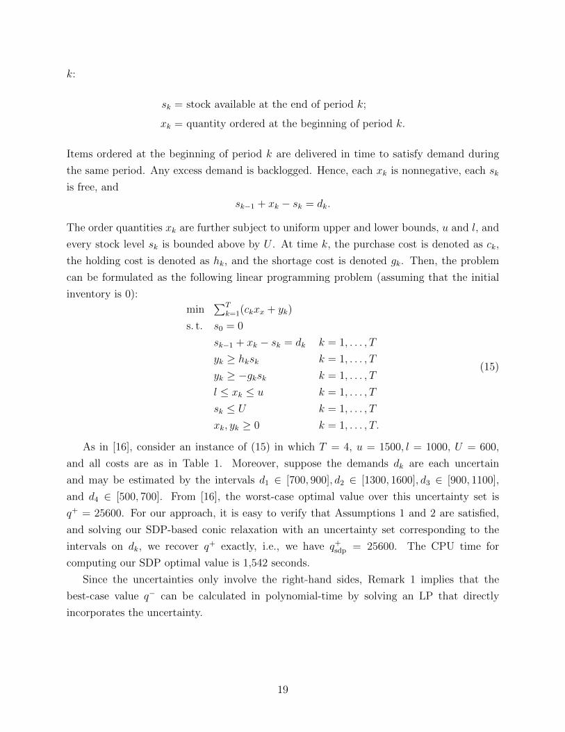
inventory is 0):
min∑T
k=1(ckxx + yk)
s. t. s0 = 0
sk−1 + xk − sk = dk k = 1, . . . , T
yk ≥ hksk k = 1, . . . , T
yk ≥ −gksk k = 1, . . . , T
l ≤ xk ≤ u k = 1, . . . , T
sk ≤ U k = 1, . . . , T
xk, yk ≥ 0 k = 1, . . . , T.
(15)
As in [16], consider an instance of (15) in which T = 4, u = 1500, l = 1000, U = 600,
and all costs are as in Table 1. Moreover, suppose the demands dk are each uncertain
and may be estimated by the intervals d1 ∈ [700, 900], d2 ∈ [1300, 1600], d3 ∈ [900, 1100],
and d4 ∈ [500, 700]. From [16], the worst-case optimal value over this uncertainty set is
q+ = 25600. For our approach, it is easy to verify that Assumptions 1 and 2 are satisfied,
and solving our SDP-based conic relaxation with an uncertainty set corresponding to the
intervals on dk, we recover q+ exactly, i.e., we have q+sdp = 25600. The CPU time for
computing our SDP optimal value is 1,542 seconds.
Since the uncertainties only involve the right-hand sides, Remark 1 implies that the
best-case value q− can be calculated in polynomial-time by solving an LP that directly
incorporates the uncertainty.
19
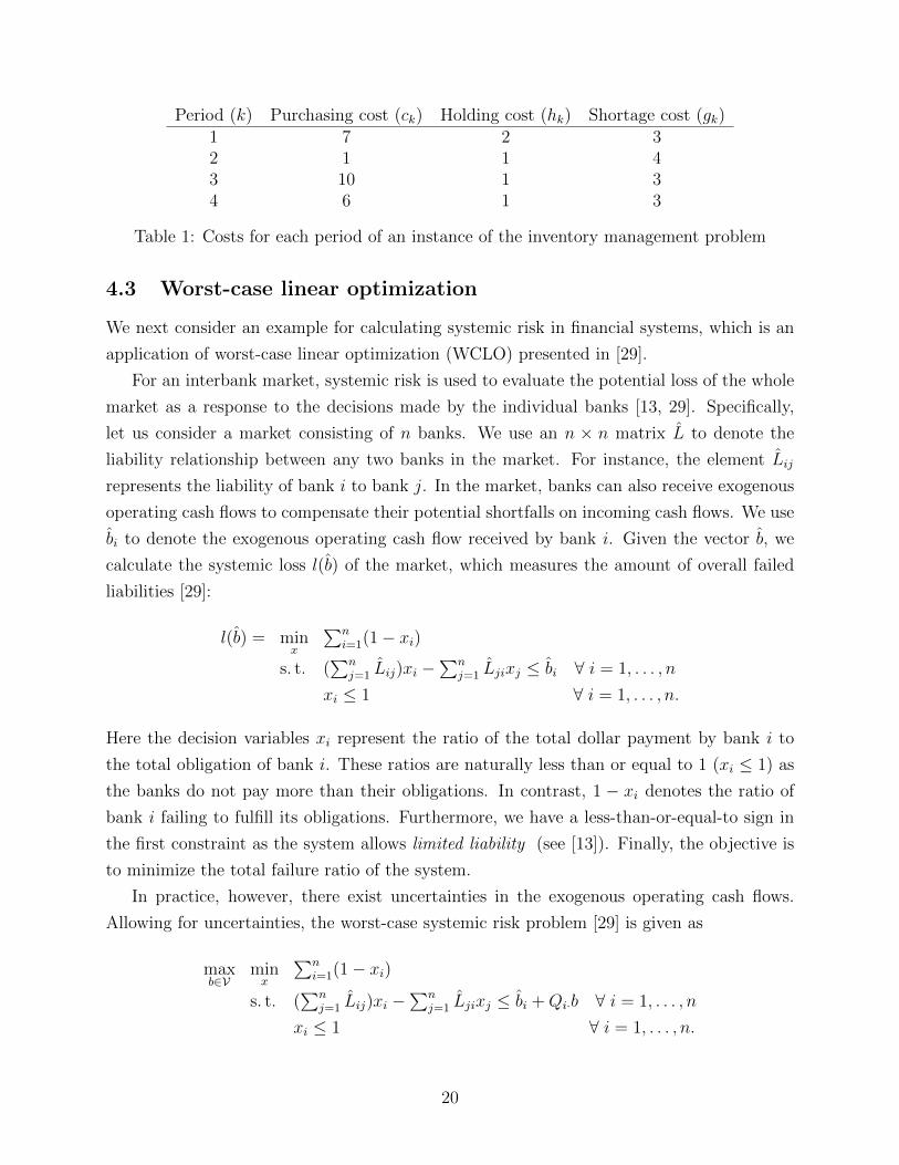
Period (k) Purchasing cost (ck) Holding cost (hk) Shortage cost (gk)1 7 2 32 1 1 43 10 1 34 6 1 3
Table 1: Costs for each period of an instance of the inventory management problem
4.3 Worst-case linear optimization
We next consider an example for calculating systemic risk in financial systems, which is an
application of worst-case linear optimization (WCLO) presented in [29].
For an interbank market, systemic risk is used to evaluate the potential loss of the whole
market as a response to the decisions made by the individual banks [13, 29]. Specifically,
let us consider a market consisting of n banks. We use an n × n matrix L to denote the
liability relationship between any two banks in the market. For instance, the element Lij
represents the liability of bank i to bank j. In the market, banks can also receive exogenous
operating cash flows to compensate their potential shortfalls on incoming cash flows. We use
bi to denote the exogenous operating cash flow received by bank i. Given the vector b, we
calculate the systemic loss l(b) of the market, which measures the amount of overall failed
liabilities [29]:
l(b) = minx
∑ni=1(1− xi)
s. t. (∑n
j=1 Lij)xi −∑n
j=1 Ljixj ≤ bi ∀ i = 1, . . . , n
xi ≤ 1 ∀ i = 1, . . . , n.
Here the decision variables xi represent the ratio of the total dollar payment by bank i to
the total obligation of bank i. These ratios are naturally less than or equal to 1 (xi ≤ 1) as
the banks do not pay more than their obligations. In contrast, 1 − xi denotes the ratio of
bank i failing to fulfill its obligations. Furthermore, we have a less-than-or-equal-to sign in
the first constraint as the system allows limited liability (see [13]). Finally, the objective is
to minimize the total failure ratio of the system.
In practice, however, there exist uncertainties in the exogenous operating cash flows.
Allowing for uncertainties, the worst-case systemic risk problem [29] is given as
maxb∈V
minx
∑ni=1(1− xi)
s. t. (∑n
j=1 Lij)xi −∑n
j=1 Ljixj ≤ bi +Qi·b ∀ i = 1, . . . , n
xi ≤ 1 ∀ i = 1, . . . , n.
20
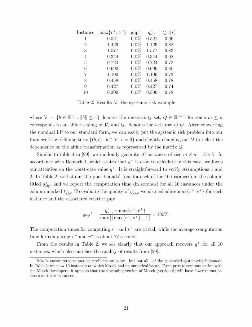
Instance max{r+, v+} gap+ q+sdp t+sdp(s)
1 0.521 0.0% 0.521 0.662 1.429 0.0% 1.429 0.823 1.577 0.0% 1.577 0.834 0.344 0.0% 0.344 0.685 0.724 0.0% 0.724 0.736 0.690 0.0% 0.690 0.807 1.100 0.0% 1.100 0.738 0.458 0.0% 0.458 0.789 0.427 0.0% 0.427 0.7410 0.300 0.0% 0.300 0.78
Table 2: Results for the systemic-risk example
where V := {b ∈ Rm : ‖b‖ ≤ 1} denotes the uncertainty set, Q ∈ Rn×m for some m ≤ n
corresponds to an affine scaling of V , and Qi· denotes the i-th row of Q. After converting
the nominal LP to our standard form, we can easily put the systemic risk problem into our
framework by defining U := {(b, c) : b ∈ V , c = 0} and slightly changing our U to reflect the
dependence on the affine transformation as represented by the matrix Q.
Similar to table 4 in [29], we randomly generate 10 instances of size m × n = 3 × 5. In
accordance with Remark 1, which states that q− is easy to calculate in this case, we focus
our attention on the worst-case value q+. It is straightforward to verify Assumptions 1 and
2. In Table 2, we list our 10 upper bounds1 (one for each of the 10 instances) in the column
titled q+sdp, and we report the computation time (in seconds) for all 10 instances under the
column marked t+sdp. To evaluate the quality of q+sdp, we also calculate max{r+, v+} for each
instance and the associated relative gap:
gap+ =q+sdp −max{r+, v+}
max{|max{r+, v+}|, 1}× 100%.
The computation times for computing r− and r+ are trivial, while the average computation
time for computing v− and v+ is about 77 seconds.
From the results in Table 2, we see clearly that our approach recovers q+ for all 10
instances, which also matches the quality of results from [29].
1Mosek encountered numerical problems on some—but not all—of the generated system-risk instances.In Table 2, we show 10 instances on which Mosek had no numerical issues. From private communication withthe Mosek developers, it appears that the upcoming version of Mosek (version 8) will have fewer numericalissues on these instances.
21
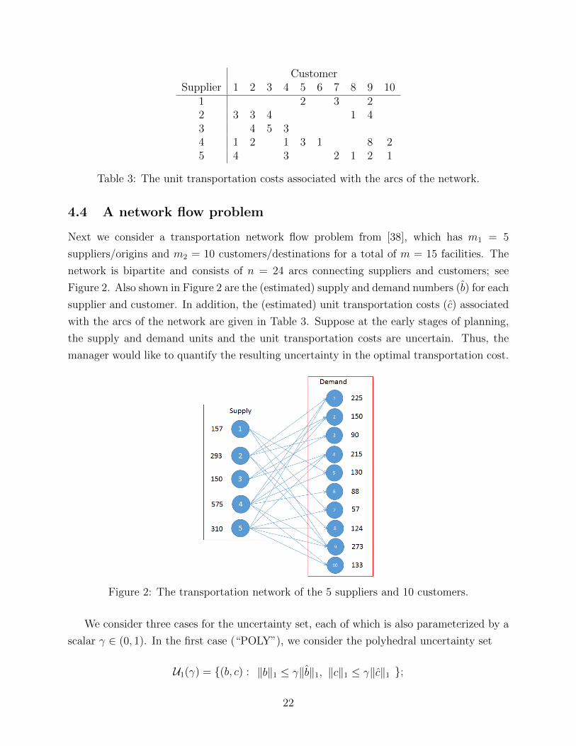
CustomerSupplier 1 2 3 4 5 6 7 8 9 10
1 2 3 22 3 3 4 1 43 4 5 34 1 2 1 3 1 8 25 4 3 2 1 2 1
Table 3: The unit transportation costs associated with the arcs of the network.
4.4 A network flow problem
Next we consider a transportation network flow problem from [38], which has m1 = 5
suppliers/origins and m2 = 10 customers/destinations for a total of m = 15 facilities. The
network is bipartite and consists of n = 24 arcs connecting suppliers and customers; see
Figure 2. Also shown in Figure 2 are the (estimated) supply and demand numbers (b) for each
supplier and customer. In addition, the (estimated) unit transportation costs (c) associated
with the arcs of the network are given in Table 3. Suppose at the early stages of planning,
the supply and demand units and the unit transportation costs are uncertain. Thus, the
manager would like to quantify the resulting uncertainty in the optimal transportation cost.
Figure 2: The transportation network of the 5 suppliers and 10 customers.
We consider three cases for the uncertainty set, each of which is also parameterized by a
scalar γ ∈ (0, 1). In the first case (“POLY”), we consider the polyhedral uncertainty set
U1(γ) = {(b, c) : ‖b‖1 ≤ γ‖b‖1, ‖c‖1 ≤ γ‖c‖1 };
22
in the second case (“SOC”), we consider the second-order-cone uncertainty set
U2(γ) := {(b, c) : ‖b‖ ≤ γ‖b‖, ‖c‖ ≤ γ‖c‖ };
and in the third case (“MIX”), we consider a mixture of the first two cases:
U3(γ) := {(b, c) : ‖b‖1 ≤ γ‖b‖1, ‖c‖ ≤ γ‖c‖ }.
For each, γ controls the perturbation magnitude in b and c relative to b and c, respectively.
In particular, we will consider three choices of γ: 0.01, 0.03, and 0.05. For example, γ = 0.03
roughly means that b can vary up to 3% of the magnitude of b. In total, we have three cases
with three choices for γ resulting in nine overall experiments.
Assumptions 1 and 2 are satisfied in this example, and so we apply our approach to
bound q− and q+; see Table 4. Our 18 bounds (lower and upper bounds for each of the nine
experiments) are listed in the two columns titled q−sdp and q+sdp, respectively. We also report
the computation times (in seconds) for all 18 instances under the two columns marked t−sdpand t+sdp. We also compute r−, v−, r+, and v+ and define the relative gaps
gap− =min{r−, v−} − q−sdp
max{|min{r−, v−}|, 1}× 100%,
gap+ =q+sdp −max{r+, v+}
max{|max{r+, v+}|, 1}× 100%.
Again, the computation times for r− and r+ are trivial. The average computation time for
computing v− and v+ is about 216 seconds.
Table 4 shows that our relaxations capture q− and q− in all cases. As ours is the first
approach to study general perturbations in the literature, we are aware of no existing methods
for this problem with which to compare our results.
4.5 The effectiveness of the redundant constraint x ◦ s = 0
Finally, we investigate the effectiveness of the redundant complementarity constraint in (10)
and (11) by also solving relaxations without the the linearized version of the constraint. As
it turns out, in all calculations of q−sdp, dropping the linearized complementarity constraint
does not change the relaxation value. However, in all calculations of q+sdp, dropping it has a
23
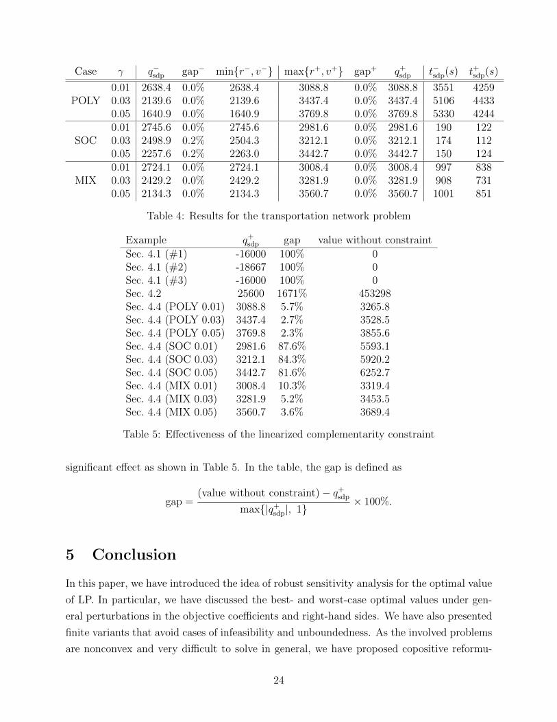
Case γ q−sdp gap− min{r−, v−} max{r+, v+} gap+ q+sdp t−sdp(s) t+sdp(s)
POLY0.01 2638.4 0.0% 2638.4 3088.8 0.0% 3088.8 3551 42590.03 2139.6 0.0% 2139.6 3437.4 0.0% 3437.4 5106 44330.05 1640.9 0.0% 1640.9 3769.8 0.0% 3769.8 5330 4244
SOC0.01 2745.6 0.0% 2745.6 2981.6 0.0% 2981.6 190 1220.03 2498.9 0.2% 2504.3 3212.1 0.0% 3212.1 174 1120.05 2257.6 0.2% 2263.0 3442.7 0.0% 3442.7 150 124
MIX0.01 2724.1 0.0% 2724.1 3008.4 0.0% 3008.4 997 8380.03 2429.2 0.0% 2429.2 3281.9 0.0% 3281.9 908 7310.05 2134.3 0.0% 2134.3 3560.7 0.0% 3560.7 1001 851
Table 4: Results for the transportation network problem
Example q+sdp gap value without constraint
Sec. 4.1 (#1) -16000 100% 0Sec. 4.1 (#2) -18667 100% 0Sec. 4.1 (#3) -16000 100% 0Sec. 4.2 25600 1671% 453298Sec. 4.4 (POLY 0.01) 3088.8 5.7% 3265.8Sec. 4.4 (POLY 0.03) 3437.4 2.7% 3528.5Sec. 4.4 (POLY 0.05) 3769.8 2.3% 3855.6Sec. 4.4 (SOC 0.01) 2981.6 87.6% 5593.1Sec. 4.4 (SOC 0.03) 3212.1 84.3% 5920.2Sec. 4.4 (SOC 0.05) 3442.7 81.6% 6252.7Sec. 4.4 (MIX 0.01) 3008.4 10.3% 3319.4Sec. 4.4 (MIX 0.03) 3281.9 5.2% 3453.5Sec. 4.4 (MIX 0.05) 3560.7 3.6% 3689.4
Table 5: Effectiveness of the linearized complementarity constraint
significant effect as shown in Table 5. In the table, the gap is defined as
gap =(value without constraint)− q+sdp
max{|q+sdp|, 1}× 100%.
5 Conclusion
In this paper, we have introduced the idea of robust sensitivity analysis for the optimal value
of LP. In particular, we have discussed the best- and worst-case optimal values under gen-
eral perturbations in the objective coefficients and right-hand sides. We have also presented
finite variants that avoid cases of infeasibility and unboundedness. As the involved problems
are nonconvex and very difficult to solve in general, we have proposed copositive reformu-
24
lations, which provide a theoretical basis for constructing tractable SDP-based relaxations
that take into account the nature of the uncertainty set, e.g., through RLT and SOC-RLT
constraints. Numerical experiments have indicated that our approach works very well on
examples from, and inspired by, the literature. In future research, it would be interesting to
improve the solution speed of the largest relaxations and to explore the possibility of also
handling perturbations in the constraint matrix.
Acknowledgments
The first author acknowledges the financial support of the AFRL Mathematical Modeling and
Optimization Institute, where he visited in Summer 2015. The second author acknowledges
the financial support of Karthik Natarajan (Singapore University of Technology and Design)
and Chung Piaw Teo (National University of Singapore), whom he visited in Fall 2014. This
research has benefitted from their many insightful comments.
References
[1] K. M. Anstreicher. Semidefinite programming versus the reformulation-linearizationtechnique for nonconvex quadratically constrained quadratic programming. Journal ofGlobal Optimization, 43(2-3):471–484, 2009.
[2] A. Ben-Tal, A. Goryashko, E. Guslitzer, and A. Nemirovski. Adjustable robust solutionsof uncertain linear programs. Math. Program. Ser. A, 99(2), 2004.
[3] D. Bertsimas and V. Goyal. On the power and limitations of affine policies in two-stageadaptive optimization. Math. Program., 134(2, Ser. A):491–531, 2012.
[4] S. P. Bradley, A. C. Hax, and T. L. Magnanti. Applied Mathematical Programming.Addison-Wesley, Reading, Mass., 1977.
[5] S. Burer. On the copositive representation of binary and continuous nonconvex quadraticprograms. Mathematical Programming, 120:479–495, 2009.
[6] S. Burer. Copositive programming. In M. Anjos and J. Lasserre, editors, Handbookof Semidefinite, Cone and Polynomial Optimization: Theory, Algorithms, Software andApplications, International Series in Operational Research and Management Science,pages 201–218. Springer, 2011.
[7] S. Burer and K. M. Anstreicher. Second-order-cone constraints for extended trust-regionsubproblems. SIAM Journal on Optimization, 23(1):432–451, 2013.
25
[8] G. B. Dantzig. Linear Programming and Extensions. Princeton University Press, Prince-ton, N.J., 1963.
[9] P. J. C. Dickinson, G. Eichfelder, and J. Povh. Erratum to: On the set-semidefiniterepresentation of nonconvex quadratic programs over arbitrary feasible sets. Optim.Lett., 7(6):1387–1397, 2013.
[10] M. Dur. Copositive Programming—A Survey. In M. Diehl, F. Glineur, E. Jarlebring,and W. Michiels, editors, Recent Advances in Optimization and its Applications in En-gineering, pages 3–20. Springer, 2010.
[11] G. Eichfelder and J. Jahn. Set-semidefinite optimization. Journal of Convex Analysis,15:767–801, 2008.
[12] G. Eichfelder and J. Povh. On the set-semidefinite representation of nonconvexquadratic programs over arbitrary feasible sets. Optim. Lett., 7(6):1373–1386, 2013.
[13] L. Eisenberg and T. H. Noe. Systemic risk in financial systems. Manag. Sci., 47(2):236–249, 2001.
[14] U. Feige, K. Jain, M. Mahdian, and V. Mirrokni. Robust combinatorial optimizationwith exponential scenarios. In Integer programming and combinatorial optimization,volume 4513 of Lecture Notes in Comput. Sci., pages 439–453. Springer, Berlin, 2007.
[15] R. M. Freund. Postoptimal analysis of a linear program under simultaneous changes inmatrix coefficients. Mathematical Programming Study, 24:1–13, 1985.
[16] V. Gabrel, C. Murat, and N. Remli. Linear programming with interval right hand sides.International Transactions in Operational Research, 17:397–408, 2010.
[17] T. Gal. Postoptimal Analyses, Parametric Programming, and Related Topics. McGraw-Hill, Hamburg, 1979.
[18] T. Gal and J. Nedoma. Multiparametric linear programming. Management Science,18(7):406–422, March 1972.
[19] D. Henrion, J. Lasserre, and J. Loefberg. Gloptipoly 3: moments, optimization andsemidefinite programming. Optim. Methods Softw., 24(4–5), 2009.
[20] M. Hladık. Interval linear programming: A survey. In Z. A. Mann, editor, LinearProgramming – New Frontiers in Theory and Applications, chapter 2, pages 85–120.Nova Science Publishers, New York, 2012.
[21] C. Kim. Parameterizing an activity vector in linear programming. Operations Research,19:1632–1646, 1971.
[22] D. Klatte. On the lower semicontinuity of the optimal sets in convex parametric opti-mization. Mathematical Programming Study, 10:104–109, 1979.
26
[23] H. Konno. A cutting plane algorithm for solving bilinear programs. MathematicalProgramming, 11:14–27, 1976.
[24] J. Lasserre. Global optimization with polynomials and the problem of moments. SIAMJ. Optim., 11(3), 2001.
[25] Z.-Q. Luo and S. Zhang. On extensions of the Frank-Wolfe theorems. Comput. Optim.Appl., 13(1-3):87–110, 1999. Computational optimization—a tribute to Olvi Mangasar-ian, Part II.
[26] P. G. McKeown and R. A. Minch. Multiplicative interval variation of objective functioncoefficients in linear programming. Management Science, 28(12):1462–1470, Decemeber1982.
[27] F. Mraz. Calculating the exact bounds of optimal values in lp with interval coefficients.Annals of Operations Research, 81:51–62, 1998.
[28] W. Orchard-Hayes. Advanced Linear-Programming Computing Techniques. McGraw-Hill, New York, 1968.
[29] J. Peng and T. Zhu. A nonlinear semidefinite optimization relaxation for the worst-caselinear optimization under uncertainties. Math. Program., 152(1, Ser. A):593–614, 2015.
[30] N. Ravi and R. E. Wendell. The tolerance approach to sensitivity analysis of matrix co-efficients in linear programming: General perturbations. The Journal of the OperationalResearch Society, 36(10):943–950, 1985.
[31] N. Ravi and R. E. Wendell. The tolerance approach to sensitivity analysis of matrixcoefficients in linear programming. Management Science, 35(9):1106–1119, September1989.
[32] H. D. Sherali and W. P. Adams. A Reformulation-Linearization Technique for SolvingDiscrete and Continuous Nonconvex Problems. Kluwer, 1997.
[33] R. E. Steuer. Algorithms for linear programming problems with interval objective func-tion coefficients. Mathematics of Operations Research, 6(3):333–348, 1981.
[34] J. E. Ward and R. E. Wendell. Approaches to sensitivity analysis in linear programming.Annals of Operations Research, 27:3–38, 1990.
[35] R. E. Wendell. A preview of a tolerance approach to sensitivity analysis in linearprogramming. Discrete Mathematics, 38:121–124, 1982.
[36] R. E. Wendell. Using bounds on the data in linear programming: The tolerance approachto sensitivity analysis. Mathematical Programming, 28:304–322, 1984.
[37] R. E. Wendell. The tolerance approach to sensitivity analysis in linear programming.Management Science, 31(5):564–578, 1985.
27
[38] F. Xie and R. Jia. Nonlinear fixed charge transportation problem by minimum costflow-based genetic algorithm. Computers and Industrial Engineering, 63:763–778, 2012.
[39] A. Takeda, S. Taguchi, and R. Tutuncu. Adjustable robust optimization models for anonlinear two-period system. J Optim Theory Appl, 136(2):275-295, 2008.
28