Robust Visual Motion Analysis: Robust Visual Motion Analysis: Piecewise-Smooth Optical FlowPiecewise-Smooth Optical Flow

Ming YeMing YeElectrical Engineering, University of Washington

mingye@u.washington.edu

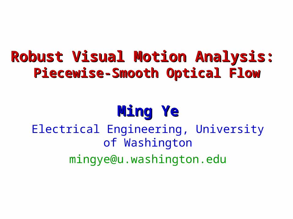
What Is Visual MotionWhat Is Visual Motion

2D image velocity 3D motion projection Temporal correspondence Image deformation

Optical flow An image of 2D velocity Each pixel Vs=(x,y) = (us,vs) where us and vs are the

displacements in x and y. (x,y,t) (x+u,y+v,t+1)

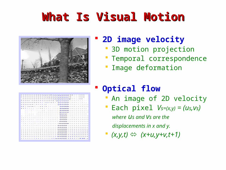
Structure From MotionStructure From Motion

Estimated horizontal motionRigid scene + camera translation

Depth map

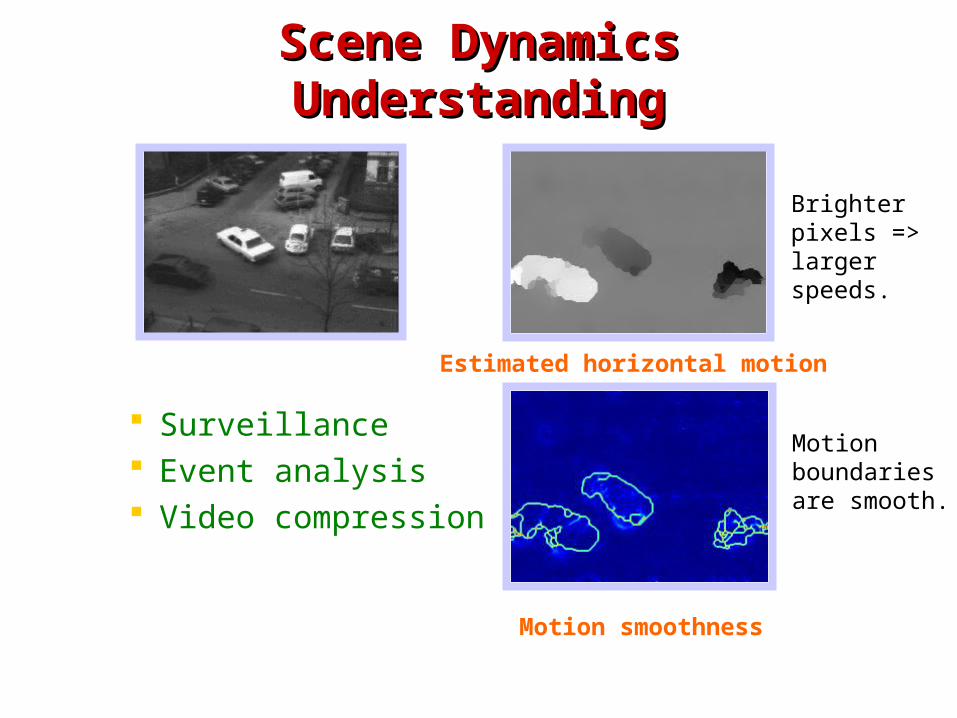
Scene Dynamics UnderstandingScene Dynamics Understanding

Surveillance Event analysis Video compression

Estimated horizontal motion

Motion smoothness

Brighter pixels =>largerspeeds.

Motionboundariesare smooth.

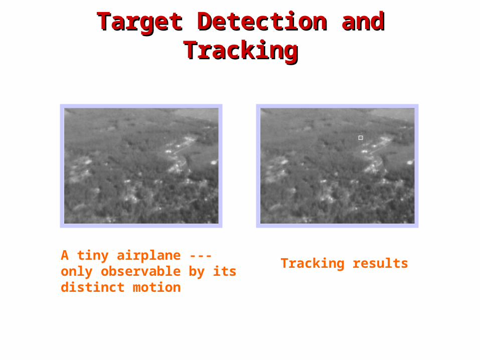
Target Detection and TrackingTarget Detection and Tracking

A tiny airplane --- only observable by its distinct motion

Tracking results

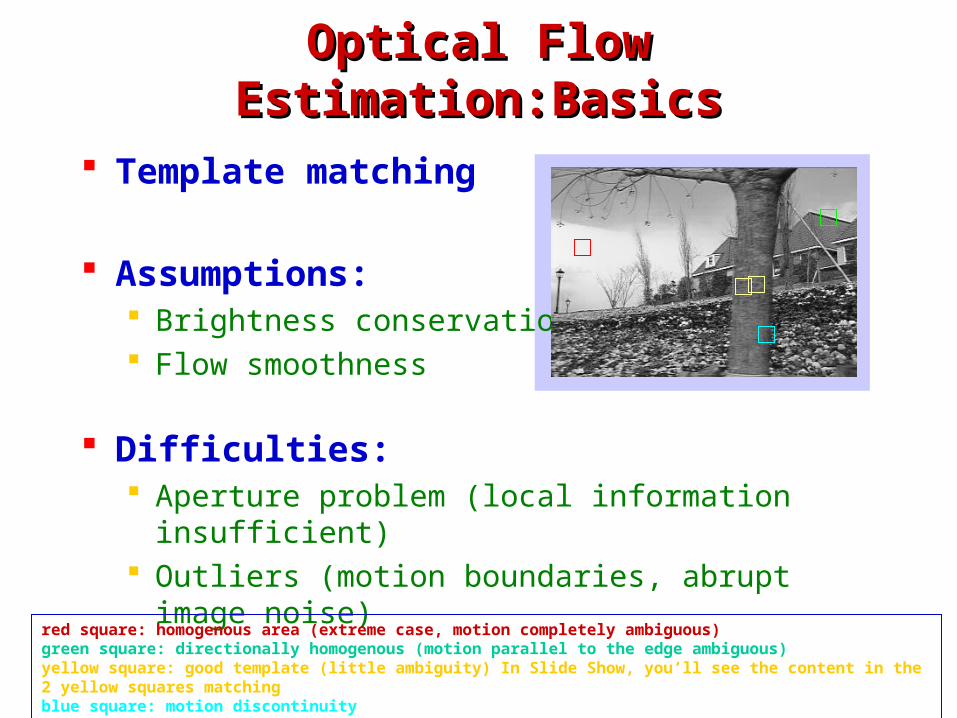
Optical Flow Estimation:BasicsOptical Flow Estimation:Basics

Template matching

Assumptions: Brightness conservation Flow smoothness

Difficulties: Aperture problem (local information insufficient) Outliers (motion boundaries, abrupt image noise)

red square: homogenous area (extreme case, motion completely ambiguous)green square: directionally homogenous (motion parallel to the edge ambiguous)yellow square: good template (little ambiguity) In Slide Show, you’ll see the content in the 2 yellow squares matchingblue square: motion discontinuity

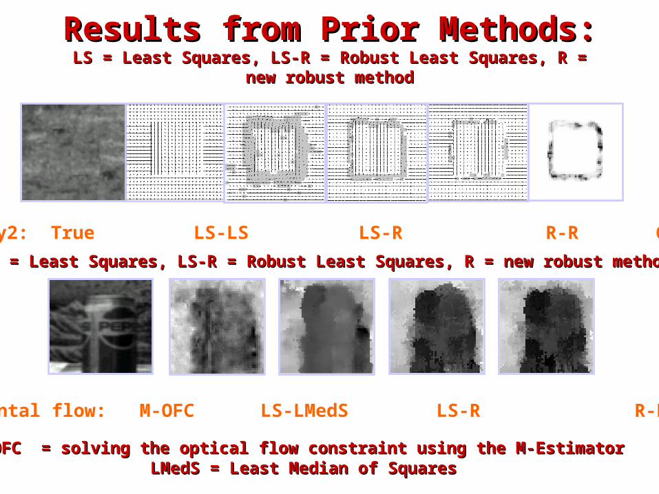
Results from Prior Methods:Results from Prior Methods:LS = Least Squares, LS-R = Robust Least Squares, R = new robust methodLS = Least Squares, LS-R = Robust Least Squares, R = new robust method

Sampled by2: True LS-LS LS-R R-R Confidence

Horizontal flow: M-OFC LS-LMedS LS-R R-R

LS = Least Squares, LS-R = Robust Least Squares, R = new robust methodLS = Least Squares, LS-R = Robust Least Squares, R = new robust method

M-OFC = solving the optical flow constraint using the M-EstimatorM-OFC = solving the optical flow constraint using the M-Estimator LMedS = Least Median of SquaresLMedS = Least Median of Squares

Estimating Piecewise-Smooth Optical Estimating Piecewise-Smooth Optical Flow with Global Matching and Flow with Global Matching and

Graduated OptimizationGraduated Optimization

A Bayesian Approach

Problem StatementProblem Statement

Assuming only brightness conservation and piecewise-smooth motion, find the optical flow to best describe the intensity change in three frames.

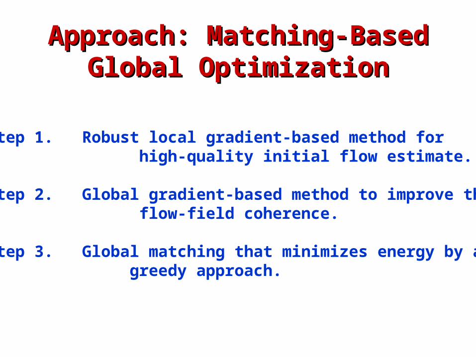
Approach: Matching-Based Approach: Matching-Based Global OptimizationGlobal Optimization

• Step 1. Robust local gradient-based method for high-quality initial flow estimate.

• Step 2. Global gradient-based method to improve the flow-field coherence.

• Step 3. Global matching that minimizes energy by a greedy approach.

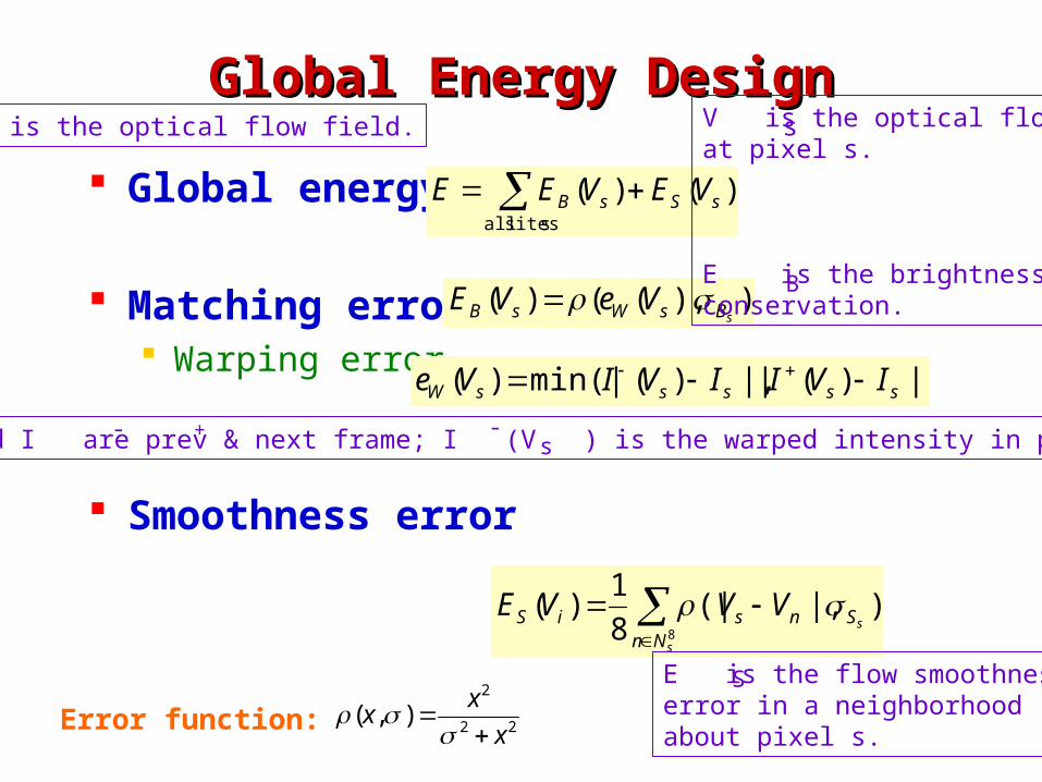
Global Energy DesignGlobal Energy Design

Global energy

Matching error Warping error

Smoothness error

s sites all

)()( sSsB VEVEE

)),(()(sBsWsB VeVE

|))(||,)(min(|)( sssssW IVIIVIVe

8

)|,(|81)(

s

sNn

SnsiS VVVE

22

2

),(x

xx

Error function:

V is the optical flow field. V is the optical flowat pixel s.

E is the brightnessconservation.

E is the flow smoothnesserror in a neighborhoodabout pixel s.

I and I are prev & next frame; I (V ) is the warped intensity in prev frame.

s

B

S

- + -s

Step 1: Gradient-Based Local RegressionStep 1: Gradient-Based Local Regression

• A crude flow estimate is assumed available (and has been compensated for)

• A robust gradient-based local regression is used to compute the incremental flow V.

• The dominant translational motion in the neighborhood of each pixel is computed by solving a set of flow equations using a least-median-of-squares criterion.

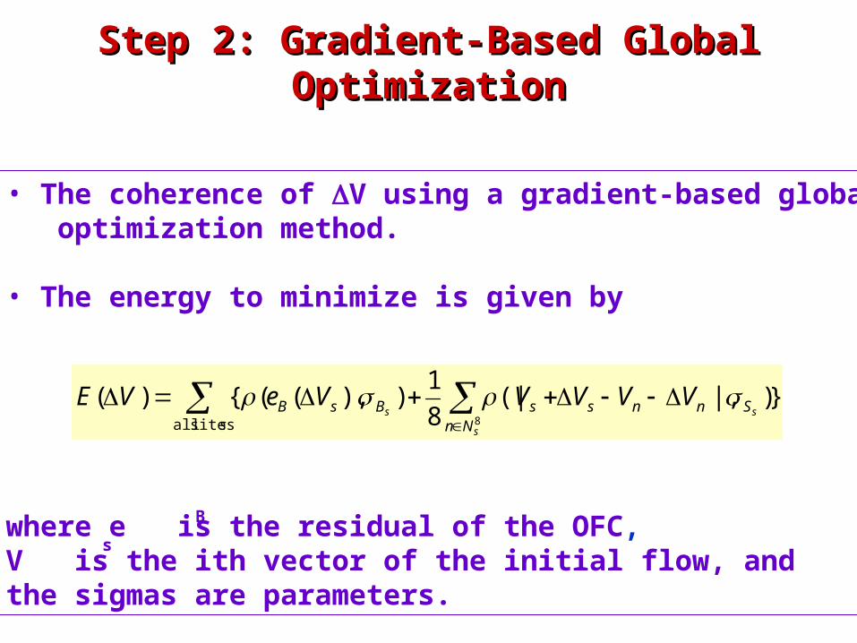
Step 2: Gradient-Based Global Step 2: Gradient-Based Global OptimizationOptimization

• The coherence of V using a gradient-based global optimization method.

• The energy to minimize is given by

where e is the residual of the OFC,V is the ith vector of the initial flow, and the sigmas are parameters.

})|,(|81)),(({)(

sites all 8

sSnns

NnsBsB s

s

sVVVVVeVE

Bs

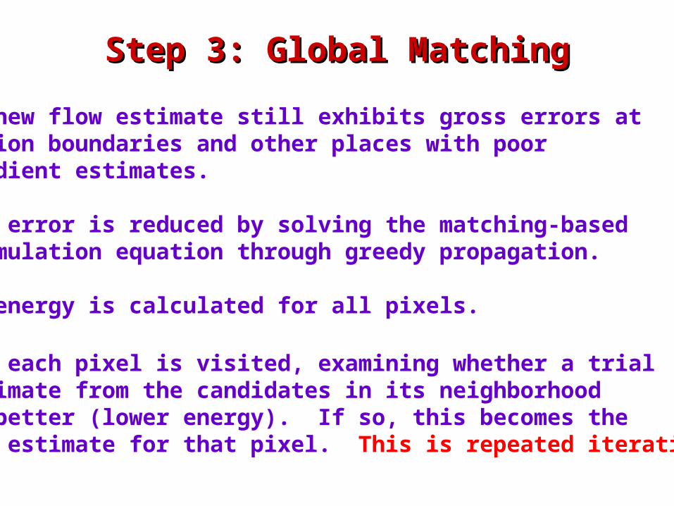
Step 3: Global MatchingStep 3: Global Matching

• The new flow estimate still exhibits gross errors at motion boundaries and other places with poor gradient estimates.

• This error is reduced by solving the matching-based formulation equation through greedy propagation.

• The energy is calculated for all pixels.

• Then each pixel is visited, examining whether a trial estimate from the candidates in its neighborhood is better (lower energy). If so, this becomes the new estimate for that pixel. This is repeated iteratively.

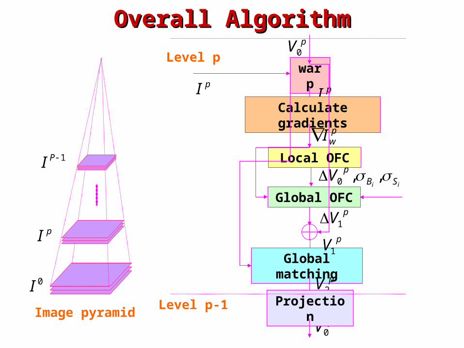
Overall AlgorithmOverall Algorithm

Image pyramid

1PI

pI

0I

10

pV

pIwarp

pwI

pV0

Calculate gradients

ii SBpV ,,0

Global matchingpV2

Projection

Level p

Level p-1

Local OFC

pwI

Global OFCpV1pV1

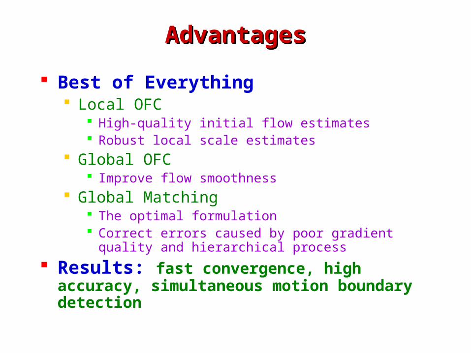
AdvantagesAdvantages

Best of Everything Local OFC

High-quality initial flow estimates Robust local scale estimates

Global OFC Improve flow smoothness

Global Matching The optimal formulation Correct errors caused by poor gradient quality and

hierarchical process Results: fast convergence, high accuracy,

simultaneous motion boundary detection

ExperimentsExperiments

• Experiments were run on several standard test videos.

• Estimates of optical flow were made for the middle frame of every three.

• The results were compared with the Black and Anandan algorithm.

TS: Translating SquaresTS: Translating Squares

Homebrew, ideal setting, test performance upper bound

64x64, 1pixel/frame

Groundtruth (cropped),Our estimate looks the same

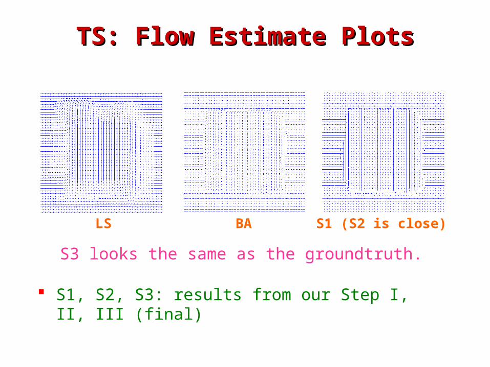
TS: Flow Estimate PlotsTS: Flow Estimate Plots

LS BA S1 (S2 is close)

S3 looks the same as the groundtruth.

S1, S2, S3: results from our Step I, II, III (final)

TT: Translating TreeTT: Translating Tree

150x150 (Barron 94)

BA 2.60 0.128 0.0724S3 0.248 0.0167 0.00984

)(e )(pix||e )(pixe BA

S3

e: error in pixels, cdf: culmulative distribution function for all pixels

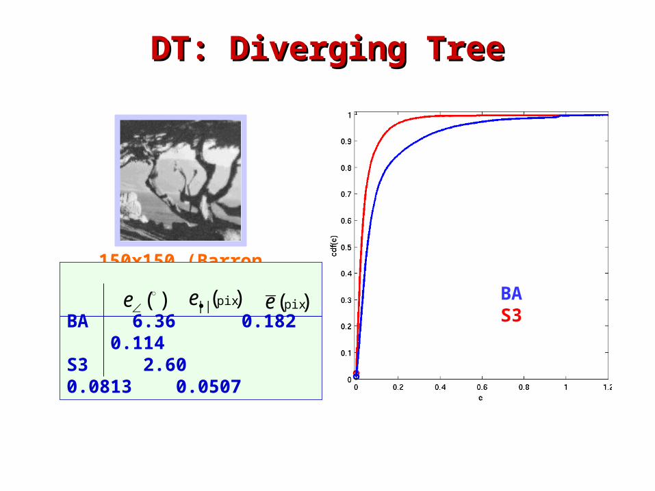
DT: Diverging TreeDT: Diverging Tree

150x150 (Barron 94)

BA 6.36 0.182 0.114S3 2.60 0.0813 0.0507

)(e )(pix||e )(pixe BA

S3

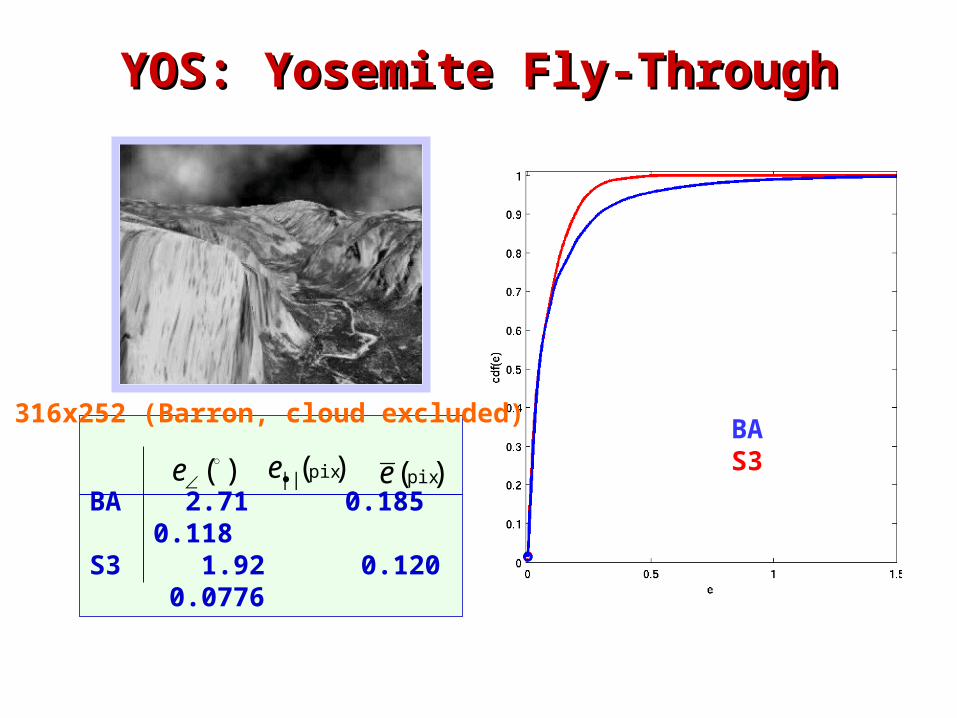
YOS: Yosemite Fly-ThroughYOS: Yosemite Fly-Through

BA 2.71 0.185 0.118S3 1.92 0.120 0.0776

)(e )(pix||e )(pixe

BAS3

316x252 (Barron, cloud excluded)

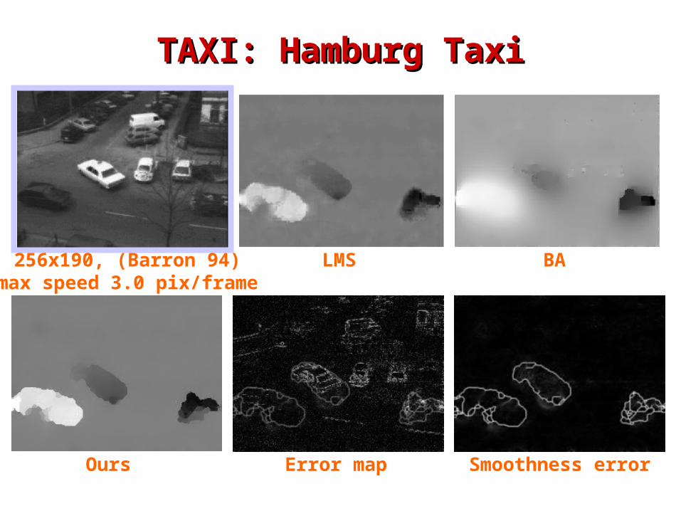
TAXI: Hamburg TaxiTAXI: Hamburg Taxi

256x190, (Barron 94)max speed 3.0 pix/frame

LMS BA

Error map Smoothness errorOurs

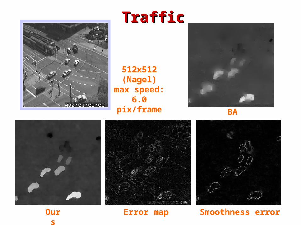
TrafficTraffic

512x512(Nagel)

max speed:6.0 pix/frame

BA

Error map Smoothness errorOurs

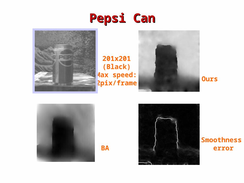
Pepsi CanPepsi Can

201x201(Black)

Max speed:2pix/frame

BA

Ours

Smoothness error

FG: Flower GardenFG: Flower Garden

360x240 (Black)Max speed: 7pix/frame

BA LMS

Error map Smoothness errorOurs

Contributions (1/2)Contributions (1/2)

Formulation More complete design, minimal parameter tuning

Adaptive local scales Strength of two error terms automatically balanced

3-frame matching to avoid visibility problems Solution: 3-step optimization

Robust initial estimates and scales Model parameter self-learning Inherit merits of 3 methods and overcome

shortcomings

Contributions (2/2)Contributions (2/2)

Results High accuracy Fast convergence By product: motion boundaries

Significance Foundation for higher-level (model-based) visual

motion analysis Methodology applicable to other low-level vision

problems