ROGUE WAVE STRUCTURE AND FORMATION MECHANISM IN …

Romanian Reports in Physics 71, 110 (2019)

ROGUE WAVE STRUCTURE AND FORMATION MECHANISM IN THE COUPLED NONLINEAR SCHRÖDINGER EQUATIONS

ZAIDONG LI1,2,*, HONGCHEN WEI2, PENGBIN HE3 1 Tianjin University of Technology, School of Science, Tianjin 300384, China

2 Hebei University of Technology, Department of Applied Physics, Tianjin 300401, China 3 Hunan University, School of Physics and Electronics, Changsha 410082, China

*Corresponding author: [email protected]

Received June 11, 2019

Abstract. By using the method of Darboux transformation, we solve the coupled nonlinear Schrödinger equations and obtain different types of exact rogue wave solutions. By adjusting the parameters of the dynamical model, we get a variety of rogue wave structures, namely bright, dark, and eye-shaped rogue waves. Also, their key characteristics are discussed in detail. We find that the non-uniform exchange rate of energy between the rogue wave and the continuous wave background can be adequately used to describe the formation mechanism of rogue waves in the coupled nonlinear Schrödinger equations.

Key words: rogue wave, coupled nonlinear Schrödinger equations, formation mechanism, non-uniform energy exchange rate.

1. INTRODUCTION

The rogue wave (RW), also known as the freak wave, is a special type of wave that looks abnormal. It was observed for the first time in the deep sea [1]; for a comprehensive review of RWs and their generating mechanisms in different physical contexts, see Ref. [2]. In recent years, RWs have aroused a great interest in natural sciences [3–7], economics, and engineering fields, especially in hydrodynamics, fiber optics, plasma physics, and Bose-Einstein condensates [6–19]. Also, the rogue waves have been reported in ultracold bosonic seas [20] and Heisenberg ferromagnetic spin chains [21]. There is no particular sign before this high-amplitude wave appears [22]. Thus RWs are extreme waves that “appear from nowhere and disappear without a trace” [11]. The amount of time when a RW appears and disappears is extremely short. Therefore, in order to prevent the potential harm of RW, the formation mechanism of such RWs and the possible manipulation of these extreme events have quickly become one of the research hotspots in the broad area of nonlinear waves [23–29]. Due to the instability of the ocean surface and the uncertainty of the environment, it is very difficult to study the RW formation in the deep ocean. The generic nonlinear Schrödinger (NLS) equation is one of the important dynamical models for studying the RW formation [30, 31]. This dynamical model and its generalizations are widely used in optics [32–39], Bose-Einstein condensation [40],

Article no. 110 Zaidong Li et al. 2

plasma physics [41], molecular biology [42] and even finance [43, 44]. Therefore, the NLS model and its generalizations to coupled systems of nonlinear partial differential equations play a very important role in the study of nonlinear wave dynamics in diverse physical settings [45–53].

In recent years, the coupled nonlinear Schrödinger (CNLS) equations have become a topic of intensive theoretical research [54–55]. There are many theoretical methods to investigate the CNLS equations, such as the analysis of the Hamiltonian structure [56], the inverse scattering method [57–59], the Darboux transformation (DT) [60–64], and the technique of conservation laws of the dynamical system [65]. Some special key features have been put forward in multi-component physical systems described by CNLS equations [66, 67].

In this paper, the CNLS equations [68–72] are solved by using the DT method, and the exact RW solutions are obtained in Sec. 2. By adjusting the parameters of the nonlinear dynamical model, we get a variety of RW structures, such as bright RWs, dark RWs, and eye-shaped RWs. Their key characteristics are discussed in detail in Sec. 3. Then, the formation mechanism of RW is explained by the non-uniform energy exchange between the RW and the continuous wave (CW) background. In Sec. 4 we give our conclusions.

2. THE ROGUE WAVE EXACT SOLUTION OF CNLS EQUATIONS

The CNLS equations with negative coherent coupling can describe the propagation of the orthogonally polarized optical waves in an isotropic medium [73]. In the paraxial approximation the CNLS equations take the form

2 2 * 21 1 1 2 1 1 2

2 2 * 22 2 2 1 2 2 1

1 2 0,21 2 0,2

t xx

t xx

iq q q q q q q

iq q q q q q q

(1)

where 1q and 2q are the slowly varying envelopes of two interacting optical modes with the asterisk being the complex conjugate. The variables x and t corresponds to the normalized distance and retarded time, respectively. In Eq. (1) the coefficients of the self-phase modulation and the cross-phase modulation are different, and the last terms in the left hand side are known as the coherent coupling terms. In fact, the coupled equations (1) describe a nonlinear dynamical model that can be integrated and its solutions can be obtained by the effective DT method. The coupled equations (1) are found to admit the Lax equations

0 1

20 1 2

,

,x

t

Ψ U U Ψ

Ψ V V V Ψ

(2)

Rogue wave structure in the coupled nonlinear Schrödinger equations Article no. 110 3

in which the compatibility condition xt txΨ Ψ yields Eq. (1). Here

†2 2 1 2

0 12 2 2 1

†2 2

0 1 2 22 2

, , ,

, , diag 1,1 ,

I O q qO QU i U i Q

O I q qQ O

I O O QV i V i I

O I Q O

2 ††2 2 2 2

22 2 2 2

1 1+ ,2 2

x

x

I O I O O QO QV iO I O I Q OQ O

and 1 2 3 4, , , TΨ φ φ φ φ or 3 41 2

32 1 4

, 1.Tφ φφ φ

Ψ δδφδφ δφ δφ

The superscript T

signifies the matrix transpose, Ψ is the matrix eigenfunction, 1,2,3,4iφ i are functions of x and t, 2 2I is the 2 2 unit matrix, O is the 2 2 zero matrix, † denotes the conjugate transpose, and λ is the eigenvalue parameter.

It is well known that the DT method is an effective technique to construct the RW solutions of Eq. (1). For this purpose, we can choose the initial seed solutions of Eq. (1) as

0 0

1 1 2 2, ,i iq a e q a e (3) which are the CW solutions and = .kx t The parameter k is the wave number of the CW, and ω is the frequency of the CW. By employing the normal process of DT we obtain the eigenfunctions of Eq. (2).

For the case of one column matrix solution, i.e., 1 2 3 4= , , , TΨ φ φ φ φ , we have

/ 2

1 1 2 1/ 2

3 3 4 3

= , ,= , ,

i

i

Γ e δiΓ e δ

(4)

where 1 2 1 3 2 1= , , ,Γ HC C Γ LC C H k iν t x with 1,2jC j being complex constants, 1/L k iν t x ν , and = λ u iν . Here the parameters u, v are the real constants. It should be noted that Eq. (1) admits two basic solutions, i.e., two CW solutions 2 1( ),a δa and one CW solution and zero solution ( 1 0a , 2 0a ). For the case of two seed CW solutions, we obtain the exact RW solution with the help of normal process of DT


0

1 1

2 1

1 4 ,

,

Jq qH

q δq

(5)

where the dispersion relation is 2 21/ 2 4ω k a . If we choose the single seed CW

solution, the exact RW solution takes the form

01 1

02 1

1 2 ,

2 ,

Jq qHJq δ qH

(6)

and the dispersion relation is 2 21= / 2ω k a . In Eq. (5) and Eq. (6), the parameters

are defined by

1 1* * 2

2 2* 2

,

2 ,

i iJ H e L e H L

H U U H L

(7)

where 1iU L H e , 1

1 2/ iC C e .

For the case of two column matrix solution, 3 41 2

32 1 4

=Tφ φφ φ

Ψδφδφ δφ δφ

, we

find that Eq. (1) should have one CW solution ( 1 0a , 2 0a ). In this case, the eigenfunction of Eq. (2) has the form

/ 2 / 21 1 2 2

/ 2 / 23 3 4 4

1 1= , ,2 2

= , ,2 2

i i

i i

Γ e Γ e

i iΓ e Γ e

(8)

where the dispersion relation is 2 21= / 2 ,ω k a and the other parameters are

1 2 1= ,Γ HC C 2 4 3= ,Γ HC C 3 2 1= ,Γ LC C 4 4 3= ,Γ LC C ,H k iν t x


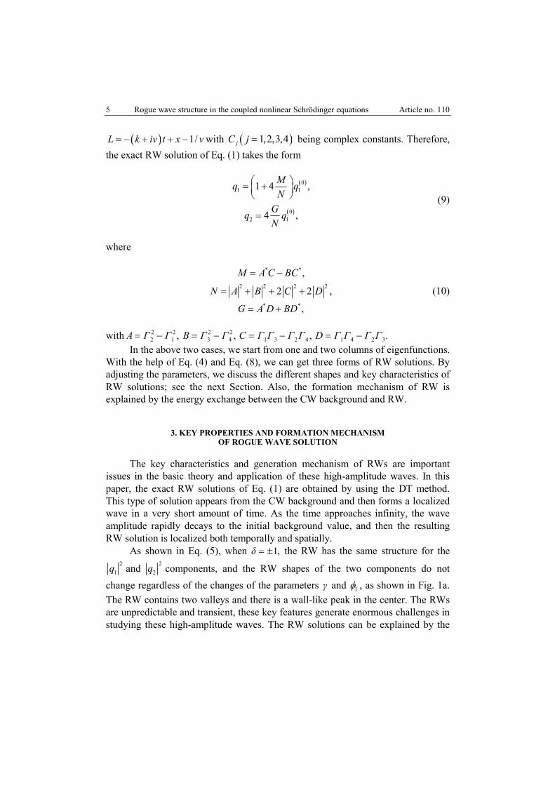
1/L k iν t x ν with 1,2,3,4jC j being complex constants. Therefore, the exact RW solution of Eq. (1) takes the form

01 1

02 1

1 4 ,

4 ,

Mq qN

Gq qN

(9)

where

* *

2 2 2 2

* *

,

2 2 ,

,

M A C BC

N A B C D

G A D BD

(10)

with 2 2

2 1 ,A Γ Γ 2 23 4 ,B Γ Γ 1 3 2 4 ,C Γ Γ Γ Γ 1 4 2 3.D Γ Γ Γ Γ

In the above two cases, we start from one and two columns of eigenfunctions. With the help of Eq. (4) and Eq. (8), we can get three forms of RW solutions. By adjusting the parameters, we discuss the different shapes and key characteristics of RW solutions; see the next Section. Also, the formation mechanism of RW is explained by the energy exchange between the CW background and RW.

3. KEY PROPERTIES AND FORMATION MECHANISM OF ROGUE WAVE SOLUTION

The key characteristics and generation mechanism of RWs are important issues in the basic theory and application of these high-amplitude waves. In this paper, the exact RW solutions of Eq. (1) are obtained by using the DT method. This type of solution appears from the CW background and then forms a localized wave in a very short amount of time. As the time approaches infinity, the wave amplitude rapidly decays to the initial background value, and then the resulting RW solution is localized both temporally and spatially.

As shown in Eq. (5), when 1,δ the RW has the same structure for the 2

1q and 22q components, and the RW shapes of the two components do not

change regardless of the changes of the parameters γ and 1 , as shown in Fig. 1a. The RW contains two valleys and there is a wall-like peak in the center. The RWs are unpredictable and transient, these key features generate enormous challenges in studying these high-amplitude waves. The RW solutions can be explained by the


energy exchange rate, which is given by Eq. (11). The energy distribution in the RW generation process is illustrated in Fig. 1b. It can be seen from Fig. 1b that the maximum value of the exchange rate of energy for the components 1q and 2q only appears once. This shows that the energy has accumulated and dissipated only once. When 0,t the energy from the CW background is gradually moving to the RW. However, when 0,t the energy of the RW gradually dissipates into the CW background. The gathering and dissipating processes of energy cause the sudden appearance and sudden disappearance of RW on the CW background, and deep troughs at both ends occur. This structure is called an eye-shaped waveform, also well known in the study of RWs in the generic NLS equation.

Fig. 1 – The illustration of vector rogue wave envelope distribution: a) components 2

1q and 22q

given by Eq. (5); b) the non-uniform energy exchange for components 1q and 2.q The parameters are 1 0.7,a 0,k = 1.4,ν = 0.4,γ 1 0.

Although there is no unified conclusion about the formation mechanism of RW, it is generally believed that the formation of RW is mainly due to the energy transfer between the RW and CW background. Thus the energy lost from the CW background is completely transferred to RW. The instability of the CW background is a prerequisite for the occurrence of RW. In order to describe quantitatively this process of energy transfer we use the non-uniform energy exchange rate

2, lim , , ,n l n nη x t q x t q x l t 1,2n to illustrate the energy conversion


between the RW and the CW background. The total non-uniform exchange rate is expressed by the integral

d .n nξ x

(11)

For the RW solution in Eq. (5), we have 2

0 1 ,nη F a 1,2,n with 2* *

0 4 8 / 8 / 16 / .F J H J H J H In the case of RW solution in Eq. (6), the non-uniform exchange rate takes the form 2

1 ,n nη F a with 2* *

1 1 2 / 2 / 4 / ,F J H J H J H and 22 4 / .F J H At last, by tedious

calculations, for the RW solution given by Eq. (9), we get ' 21n nη F a with

2' * *1 4 8 / +8 / 16 / ,F M N M N M N and 2'

2 16 / .F G N

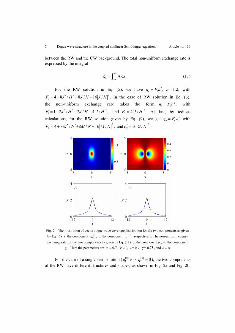
Fig. 2 – The illustration of vector rogue wave envelope distribution for the two components as given by Eq. (6): a) the component 2

1 ;q b) the component 22 ,q respectively. The non-uniform energy

exchange rate for the two components as given by Eq. (11): c) the component 1;q d) the component

2.q Here the parameters are 1 0.7,a 0,k = 0.7,ν = 0.75γ , and 0.

For the case of a single seed solution ( 01 0,q 0

2 0q ), the two components of the RW have different structures and shapes, as shown in Fig. 2a and Fig. 2b.


The expression of the RW solution is given by Eq. (6). As can be seen from Fig. 2a, the component 2

1q is a bright RW with a peak. Figure 2b shows the component 2

2 ,q which is a dark RW with two troughs. We see from Fig. 2c and Fig. 2d that the energy exchange rates of the components 1q and 2q have the same structure, describing the accumulation and dissipation of energy leading to the sudden appearance and disappearance of RW. At a certain moment of time, the energy is concentrated. At 0,t the energy density of the RW is the highest, corresponding to the peaks and valleys of the RW. Thus the physical mechanism that produces RW is the continuous accumulation of energy towards the central portion of the waveform.

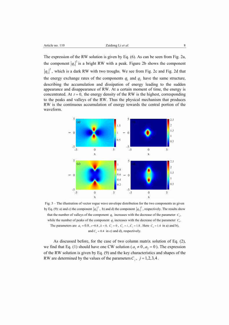
Fig. 3 – The illustration of vector rogue wave envelope distribution for the two components as given

by Eq. (9): a) and c) the component 21 ,q b) and d) the component 2

2q , respectively. The results show that the number of valleys of the component 1q increases with the decrease of the parameter 4 ,C while the number of peaks of the component 2q increases with the decrease of the parameter 4 .C

The parameters are 1 0.8a , =0.8ν , 0,k 1 0C , 2C i , 3 1.8C . Here 4 1.4C in a) and b), and 4 0.4C in c) and d), respectively.

As discussed before, for the case of two column matrix solution of Eq. (2), we find that Eq. (1) should have one CW solution ( 1 0a , 2 0a ). The expression of the RW solution is given by Eq. (9) and the key characteristics and shapes of the RW are determined by the values of the parameters jC , 1,2,3,4j .


Firstly, we consider the case when 1 0C . We keep the parameters 2C and

3C unchanged, and we only adjust the parameter 4C , so we can get two different RW shapes, as shown in Fig. 3. As can be seen from Fig. 3a and Fig. 3c, a localized RW appears on the CW background. And because the amplitude of the CW background is smaller than the amplitude of the RW, the RW has a high energy characteristic. Although the peaks and troughs suddenly appear in the CW background, the entire physical system is conservative because the depression of troughs is exactly balanced by the protrusion of peaks. In Fig. 3a, the 2

1q component has a structure of two peaks and two valleys, whereas the RW shown in Fig. 3c has two peaks and four valleys. When the amplitude of the CW is 2 0a ,

the seed solution of the CW degenerates into the zero solution ( 02 0q ), at which

point we get a bright RW, as shown in Fig. 3b and Fig. 3d. In Fig. 3b, the RW is excited at , 0,0x t , and the RW has a single peak. As the parameter 4C decreases, there occur two peaks in the RW, see Fig. 3d.

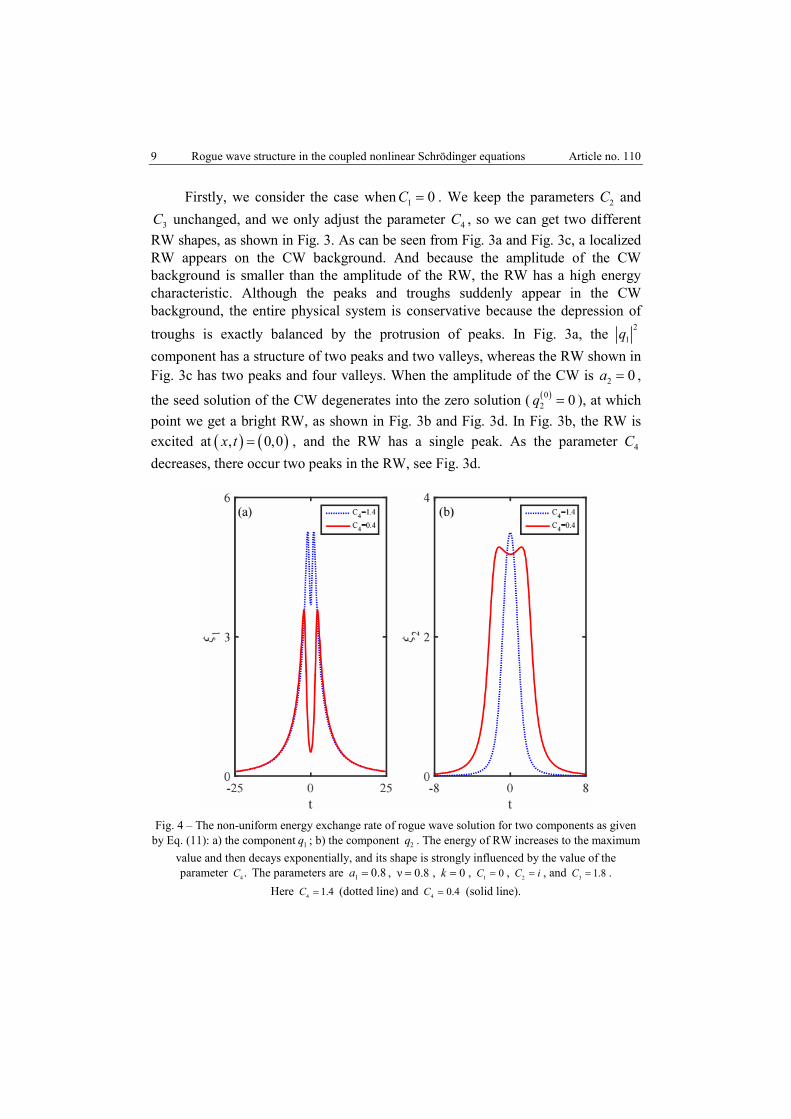
Fig. 4 – The non-uniform energy exchange rate of rogue wave solution for two components as given

by Eq. (11): a) the component 1q ; b) the component 2q . The energy of RW increases to the maximum value and then decays exponentially, and its shape is strongly influenced by the value of the parameter 4 .C The parameters are 1 0.8a , ν 0.8 , 0k , 1 0C , 2C i , and 3 1.8C .

Here 4 1.4C (dotted line) and 4 0.4C (solid line).


In order to investigate the properties of RW illustrated in Fig. 3, we plot the total energy exchange rate nξ , 1,2n , for the components 1q and 2q , as shown in Fig. 4. The accumulation and attenuation of energy can be clearly seen from Fig. 4. Figure 4a shows that the RW absorbs energy from the CW background. Two maximum values appear successively, and the aggregation of energy occurs twice. This process results in the appearance of two peaks with the generation of troughs, see Fig. 3a and Fig. 3c. Then, the energy is gradually dissipated into the CW background.

It should be noted that the existence of RW solution for the component 2q comes from the coherent coupling term in Eq. (1) because of the existence of single seed solution ( 0

1 0q , 02 =0q ). With the change of the parameter 4C , the energy

exchange rate has a different structure, see Fig. 4b. When 4 1.4C , the energy of the RW increases to the maximum value and then decays exponentially, the aggregation and dissipation of energy occur only once. It leads to the generation of a single peak, as shown in Fig. 3b. And when 4 0.4C , the whole process of energy accumulation and dissipation leads to the formation of two peaks, as shown in Fig. 3d. The rogue wave is unstable, as illustrated by the sharp increase and decrease of energy in Fig. 4.

Secondly, we consider the general case when 0jC , 1,2,3,4.j For example, we keep the parameters 1C , 2C , and 4C unchanged and by adjusting the parameter 3C , we can get the RW structure of the components 1q and 2q , as shown in Fig. 5. It shows the RW structure in the time and space domains. The RW is an unusually large waveform contained in a random wave train. It has obvious nonlinear key feature: a short duration, the RW energy is localized, implying an amazing destructive power. Figures 5 a and 5 c represent the 2

1q component, and

Figs. 5b and 5d represent the 22q component. When 3 0.1C , the 2

1q component has a peak and two valleys; the peaks are thin and the valleys are flat, showing the obvious peak-valley asymmetry as illustrated in Fig. 5a. When 3 1.3C , the 2

1q component has one peak and three valleys, as shown in Fig. 5c. Since Eq. (1) is a CNLS equation with a seed solution ( 0

1 0q , 02 0q ), and the CW amplitude has

the value 2 0a , the CW background of the 22q component is zero. The RW of the

22q component is localized in time and in propagation direction, and is surrounded

by a zero background. When 3 0.1C or 3 1.3C , the 22q component is a bright

RW with two peaks. When 3C increases, the distance between the two peaks becomes larger, as shown in Figs. 5 b and 5 d, respectively.


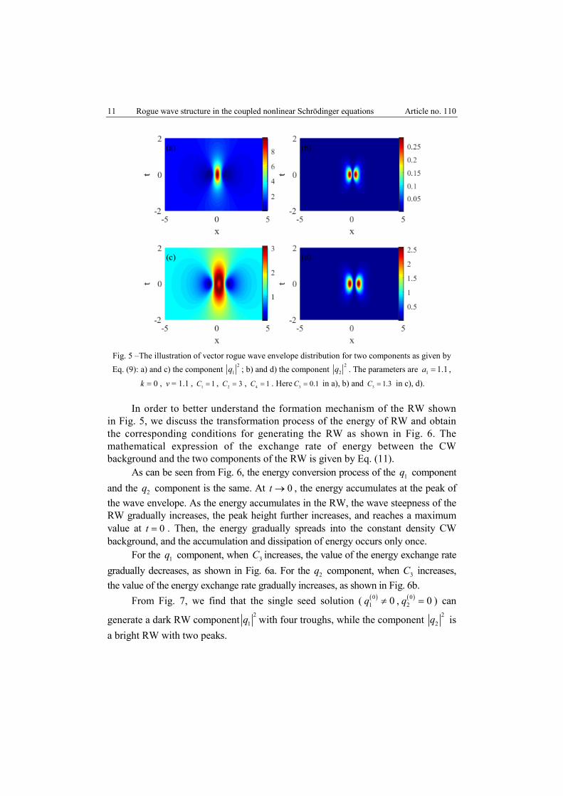
Fig. 5 –The illustration of vector rogue wave envelope distribution for two components as given by Eq. (9): a) and c) the component 2

1q ; b) and d) the component 22q . The parameters are 1 1.1a ,

0k , = 1.1ν , 1 1C , 2 3C , 4 1C . Here 3 0.1C in a), b) and 3 1.3C in c), d).

In order to better understand the formation mechanism of the RW shown in Fig. 5, we discuss the transformation process of the energy of RW and obtain the corresponding conditions for generating the RW as shown in Fig. 6. The mathematical expression of the exchange rate of energy between the CW background and the two components of the RW is given by Eq. (11).

As can be seen from Fig. 6, the energy conversion process of the 1q component and the 2q component is the same. At 0t , the energy accumulates at the peak of the wave envelope. As the energy accumulates in the RW, the wave steepness of the RW gradually increases, the peak height further increases, and reaches a maximum value at 0t . Then, the energy gradually spreads into the constant density CW background, and the accumulation and dissipation of energy occurs only once.

For the 1q component, when 3C increases, the value of the energy exchange rate gradually decreases, as shown in Fig. 6a. For the 2q component, when 3C increases, the value of the energy exchange rate gradually increases, as shown in Fig. 6b.

From Fig. 7, we find that the single seed solution ( 01 0q , 0

2 0q ) can

generate a dark RW component 21q with four troughs, while the component 2

2q is a bright RW with two peaks.


Fig. 6 – The non-uniform energy exchange rate of rogue waves for the two components as given by Eq. (11): a) for component 1q ; b) for component 2q . The parameters are 1 1.1a , = 1.1ν , 0k ,

1 1C , 2 3C , 4 1C . Here 3 1.3C (dotted line) and 3 0.1C (solid line).

Fig. 7 – The illustration of vector rogue wave envelope distribution for the two components as given in Eq. (9): (a), (b), and (c) the component 2

1q ; (d), (e), and (f) the component 22q . The parameters

are 1 1a , 1ν , 1 1.4C , 2 2C , 3 3.5C , and 4 1C . Here 1k in (a), (d); 0k in (b), (e); and 1k in (c), (f).


We find that the parameter k controls the rotation of RW. When 0k , the RW corresponding to the components 2

1q and 22q is rotated to the left, as shown

in Figs. 7a and 7d. When 0k , the two components rotate to the right as shown in Figs. 7c and 7f. As the wave number k changes, although the amplitude of the RW does not change, the RW width gradually narrows as k increases. Therefore, the wave number k of the CW can not only control the rotation of RW, but also control the width of RW.

4. CONCLUSIONS

In this paper, the Darboux transformation method has been used to solve the CNLS equations and the families of exact RW solutions are obtained through a series of tedious calculations. By adjusting the parameters of the physical model, different types of RWs are obtained, and their key characteristics are analyzed in detail.

In order to better understand the formation mechanism of the obtained RW solutions of the CNLS equations, a non-uniform exchange rate of energy between the RW and the CW background is introduced and calculated numerically for different sets of the values of the parameters of the nonlinear dynamical model. The main reason for the formation of RWs is the accumulation of energy in very limited space and time intervals.

The results of this study offer a better understanding of the intrinsic nature and the formation mechanism of RWs, and can help in controlling the RW dynamics in other relevant physical settings.

Acknowledgements. This work was supported by the National Natural Science Foundation of

China (Grant No. 61774001), and the Program of State Key Laboratory of Quantum Optics and Quantum Optics Devices (No. KF201906). Peng-Bin He was supported by the NSF of Hunan Province through grant No. 2017JJ2045.

REFERENCES

1. L. Draper, Oceanus 10, 12 (1964). 2. M. Onorato, S. Residori, U. Bortolozzo, A. Montina, and F. T. Arecchi, Phys. Rep. 528, 47 (2013). 3. Z. D. Li, Q. Y. Li, T. F. Xu, and P. B. He, Phys. Rev. E 94, 042220 (2016). 4. N. Akhmediev and E. Pelinovsky, Eur. Phys. J. Spec. Top. 185, 1 (2010). 5. S. Chen, F. Baronio, J. M. Soto-Crespo, P. Grelu, and D. Mihalache, J. Phys. A: Math. Theor. 50,

463001 (2017). 6. D. Mihalache, Rom. Rep. Phys. 69, 403 (2017). 7. B. A. Malomed and D. Mihalache, Rom. J. Phys. 64, 106 (2019). 8. D. R. Solli, C. Ropers, P. Koonath, and B. Jalali, Nature 450, 1054 (2007). 9. Z. D. Li, Q. Y. Li, and W. M. Liu, J. Phys.: Conf. Ser. 827, 012002 (2017).


10. N. Akhmediev, A. Ankiewicz, J. M. Soto-Crespo, and J. M. Dudley, Phys. Lett. A 375, 541 (2011). 11. N. Akhmediev, A. Ankiewicz, and M. Taki, Phys. Lett. A 373, 675 (2009). 12. B. L. Guo and L. M. Ling, Chin. Phys. Lett. 28, 110202 (2011). 13. Q. Y. Li, F. Zhao, P. B. He, and Z. D. Li, Chin. Phys. B 24, 037508 (2015). 14. C. Q. Dai, Y. Y. Wang, Q. Tian, and J. F. Zhang, Ann. Phys. 327, 512 (2012). 15. Z. Y. Yang, L. C. Zhao, T. Zhang, Y. H. Li, and R. H. Yue, Opt. Commun. 283, 3768 (2010). 16. V. I. Kruglov, A. Peacock, and J. D. Harvey, Phys. Rev. Lett. 90, 113902 (2003). 17. S. Ponomarenko and G. P. Agrawal, Opt. Lett. 32, 1659 (2007). 18. J. He, S. Xu, and K. Porsezian, J. Phys. Soc. Jpn. 81, 3002 (2012). 19. W. M. Moslem, P. K. Shukla, and B. Eliassoni, EPL 96, 25002 (2011). 20. E. G. Charalampidis, J. Cuevas-Maraver, D. J. Frantzeskakis, and P. G. Kevrekidis, Rom. Rep.

Phys. 70, 504 (2018). 21. W. Liu, Rom. J. Phys. 62, 118 (2017). 22. B. Guo, L. Ling, and Q. P. Liu, Phys. Rev. E 85, 026607 (2012). 23. Z. Y. Yan, Phys. Lett. A 374, 672 (2010). 24. B. Kibler, J. Fatome, C. Finot, G. Genty, N. Akhmediev, and J. M. Dudley, Nat. Phys. 6, 790 (2010). 25. A. Chabchoub, N. P. Hoffmann, and N. Akhmediev, Phys. Rev. Lett. 106, 204502 (2011). 26. A. Chabchoub, N. Hoffmann, M. Onorato, and N. Akhmediev, Phys. Rev. X 2, 011015 (2012). 27. A. Chabchoub, N. Hoffmann, M. Onorato, A. Slunyaev, E. Pelinovsky, and N. Akhmediev, Phys.

Rev. E 86, 056601 (2012). 28. Y. V. Bludov, V. V. Konotop, and N. Akhmediev, Phys. Rev. A 80, 033610 (2009). 29. Z. Y. Qin and G. Mu, Phys. Rev. E 86, 036601 (2012). 30. G. Y. Yang, L. Li, S. T. Jia, and D. Mihalache, Rom. Rep. Phys. 65, 391 (2013). 31. G. Y. Yang, L. Li, S. T. Jia, and D. Mihalache, Rom. Rep. Phys. 65, 902 (2013). 32. B. A. Malomed, D. Mihalache, F. Wise, and L. Torner, J. Opt. B: Quantum Semiclass. Opt. 7, R53

(2005). 33. B. Malomed, L. Torner, F. Wise, and D. Mihalache, J. Phys. B: At. Mol. Opt. Phys. 49, 170502 (2016). 34. Y. V. Kartashov, G. E. Astrakharchik, B. A. Malomed, and L. Torner, Nat. Rev. Phys. 1, 185

(2019). 35. Y. Xiao, Z. Y. Xu, L. Li, and Z. H. Li, J. Nonlinear Opt. Phys. 12, 341 (2003). 36. L. Li, Z. H. Li, S. Q. Li, and G. S. Zhou, Opt. Commun. 234, 169 (2004). 37. S. Chen, Y. Zhou, L. Bu, F. Baronio, J. M. Soto-Crespo, and D. Mihalache, Opt. Express 27,

11370 (2019). 38. S. Chen and D. Mihalache, J. Phys. A: Math. Theor 48, 215202 (2015). 39. B. Kibler, J. Fatome, C. Finot, G. Millot, G. Genty, B. Wetzel, N. Akhmediev, F. Dias, and

J. M. Dudley, Sci. Rep. 2, 463 (2012). 40. E. P. Bashkin and A. V. Vagov, Phys. Rev. B 56, 6207 (1997). 41. H. Bailung and Y. Nakamura, J. Plasma, Phys. 50, 231 (1993). 42. A. C. Scott, Physica Scripta 29, 279 (1984). 43. Z. Y. Yan, Commun. Theor. Phys. 54, 947 (2010). 44. Z. Y. Yan, Phys. Lett. A 375, 4274 (2011). 45. M. J. Ablowitz and Z. H. Musslimani, Phys. Rev. Lett. 110, 064105 (2013). 46. L. C. Zhao and L. Ling, Phys. Rev. E 92, 022924 (2015). 47. A. V. Mikhailov, A. B. Shabat, and R. I. Yamilov, Russ. Math. Surv. 42, 1 (1987). 48. C. Becker, S. Stellmer, P. S. Panahi, S. Dörscher, E. Richter, J. Kronjäger, K. Bongs, and

K. Sengstock, Nat. Phys. 4, 496 (2008). 49. T. Kanna and M. Lakshmanan, Phys. Rev. Lett. 86, 5043 (2001). 50. T. Kanna, M. Vijayajayanthi, and M. Lakshmanan, Phys. Rev. A 77, 013820 (2008). 51. L. C. Zhao and J. Liu, J. Opt. Soc. Am. B 29, 3119 (2012). 52. Z. Yan and C. Dai, J. Opt. 15, 064012 (2013). 53. Z. Yan, Appl. Math. Lett. 47, 61 (2015). 54. G. Zhang, Z. Yan, X. Y. Wen, and Y. Chen, Phys. Rev. E 95, 042201 (2017).


55. M. Vijayajayanthi, T. Kanna, and M. Lakshmanan, Phys. Rev. A 76, 013808 (2007). 56. J. Williams, R. Walser, J. Cooper, E. Cornell, and M. Holland, Phys. Rev. A 59, R31 (1998). 57. X. J. Chen and W. K. Lam, Phys. Rev. E 69, 066604 (2004). 58. X. J. Chen and J. Yang, Phys. Rev. E 65, 066608 (2002). 59. J. Lenells, Physica D 237, 3008 (2008). 60. H. Steudel, J. Phys. A: Math. Gen. 36, 1931 (2003). 61. Y. Xiao, J. Phys. A: Gen. Phys. 24, 363 (1991). 62. V. E. Vekslerchik, J. Phys. A: Math. Theor. 44, 465207 (2011). 63. B. Guo, L. Ling, and Q. P. Liu, Stud. Appl. Math. 130, 317 (2013). 64. X. Y. Wen, Y. Yang, and Z. Yan, Phys. Rev. E 92, 012917 (2015). 65. L. Xing and M. Peng, Commun. Nonlinear Sci. Numer. Simul. 18, 2304 (2013). 66. L. Xing, Nonlinear Dyn. 81, 239 (2015). 67. Y. V. Bludov, V. V. Konotop, and N. Akhmediev, Eur. Phys. J. Spec. Top. 185, 169 (2010). 68. J. Williams, R. Walser, J. Cooper, E. A. Cornell, and M. Holland, Phys. Rev. A 61, 033612 (1999). 69. M. G. Forest, D. W. Mclaughlin, D. J. Muraki, and O. C. Wright, J. Nonl. Sci. 10, 291 (2000). 70. A. Ankiewicz, N. Akhmediev, and J. M. Soto-Crespo, Phys. Rev. E 80, 026601 (2009). 71. L. Ling and Q. P. Liu, J. Phys. A: Math. Theor. 43, 434023 (2010). 72. G. Y. Yang, Y. Wang, Z. Y. Qin, B. A. Malomed, D. Mihalache, and L. Li, Phys. Rev. E 90,

062909 (2014). 73. B. A. Malomed, Phys. Rev. A 45, 8321(R) (1992).


Documents

ROGUE WAVE STRUCTURE AND FORMATION MECHANISM IN …