Romanian Reports in Physics, Vol. 68, No. 4, P. 1425–1446 ... · Romanian Reports in Physics, Vol. 68, No. 4, P. 1425–1446, ... eral fundamental rogue waves and which consist

Romanian Reports in Physics, Vol. 68, No. 4, P. 1425–1446, 2016

PARALLEL LINE ROGUE WAVES OF THE THIRD-TYPEDAVEY-STEWARTSON EQUATION

YAOBIN LIU1, A. S. FOKAS2, D. MIHALACHE3, JINGSONG HE1,∗

1Department of Mathematics, Ningbo University, Ningbo, Zhejiang 315211, P. R. China∗Corresponding author, E-mail: [email protected]

2University of Cambridge, Department of Applied Mathematics and Theoretical Physics, CambridgeCB3 0WA, England

3Horia Hulubei National Institute for Physics and Nuclear Engineering, RO-077125,Bucharest-Magurele, Romania

Received July 25, 2016

Abstract. An explicit form of rogue waves of the third-type Davey-Stewartson(DSIII) equation is derived using the bilinear transformation method. The relevant for-mulas involve determinants whose matrix elements are simple polynomials. It is shownthat the simplest (fundamental) rogue waves are line rogue waves that arise from a con-stant background at t 0 and then retreat back to a constant background at t 0.Higher-order waves are parallel line rogue waves that describe the interaction of sev-eral fundamental rogue waves and which consist of several parallel lines. A dark roguewave, which reaches a deep amplitude below the asymptotical background, is also ex-plicitly constructed. Several differences between the rogue waves of the DSIII equationand those of the DSI equation are discussed, and are also illustrated graphically.

Key words: Davey-Stewartson III equation, bilinear transformation method,rogue wave.

PACS: 02.30.Ik, 02.30.Jr, 05.45.Yv

1. INTRODUCTION

In recent years, rogue waves (RWs), which are a novel type of rational solitarywaves, have generated much interest in both mathematics and physics. Rogue waveswere first observed in deep ocean [1–3] and later in optical fibres [4, 5], in water tanks[6, 7], and in several other physical settings [8, 9]. Rogue waves are generated viathe modulation instability of monochromatic waves and have the fascinating propertythat they seem to appear “out of nowhere” and disappear “without trace” [10]. Thebasic properties of RWs are summarized in [11]: (i) the RWs are (quasi-) rationalsolutions; (ii) they are localized in both time and space; and (iii) they have largeamplitudes allocated with two hollows (the RW peak has a height of at least threetimes of the background). These generic features are considered as the ‘definition’of the first-order RW solution.

There exist only few (2+1)-dimensional soliton equations that have rogue wave

(c) 2016 RRP 68(No. 4) 1425–1446 - v.1.1a*2016.11.24

1426 Yaobin Liu et al. 2

solutions [12–19]. This fact motivates us to seek rogue waves for the third-typeDavey-Stewartson (DSIII) equation. This equation is given by

iqt− qxx+ qyy−2λq[(

∫ x

−∞|q|2ydx′+u1(y,t))− (

∫ y

−∞|q|2xdy′+u2(x,t))] = 0,

(1)where λ = ±1, the complex-valued scalar function q(x,y, t) represents a certainphysical quantity and u1(y,t) and u2(x,t) are two arbitrary real-valued functions.Using the transformations

Vx = |q|2y, V =

∫ x

−∞|q|2ydx′+u1(y,t), (2a)

and

Uy = |q|2x, U =

∫ y

−∞|q|2xdy′+u2(x,t), (2b)

Eq. (1) becomes the following system of coupled partial differential equations:

iqt− qxx+ qyy−2λq(V −U) = 0, (3a)

Vx = |q|2y, (3b)

Uy = |q|2x, (3c)where V and U are two real functions.

This equation was obtained by Boiti et al. [20] employing ideas [21] of the so-called direct linearising method of Fokas and Ablowitz [22]. However, as noted byFokas[23], it was derived earlier by Schulman [24] and by Fokas and Santini [25, 26]using the symmetry approach.

Equation (1) supports localized solutions such as lump solitons. In this paper,we derive an explicit representation for the rogue wave solutions of DSIII equation(3) and also discuss the differences between the rogue wave solutions of the DSIIIequation and those of the DSI equation.

This paper is organised as follows. In Sec. 2, our main result is derived, whichcan be used to express rogue wave solutions of Eq. (3) in terms of determinants ofN ×N matrices. The dynamics of rogue wave solutions are discussed at Sec. 3. Ourresults are summarised in Sec. 4.

2. ROGUE WAVE SOLUTION VIA DETERMINANTS OF N ×N MATRICES

In this Section, we derive an explicit form of the rogue waves for Eq. (3). Usingthe dependent variable transformations

q = g/f, V =−λ(logf)yy, U =−λ(logf)xx, (4)

(c) 2016 RRP 68(No. 4) 1425–1446 - v.1.1a*2016.11.24

3 Parallel line rogue waves of the third-type Davey-Stewartson equation 1427

the DSIII equation can be transformed into the bilinear forms

(iDt−Dx2 +Dy

2)g ·f = 0,

(λDxDy−2)f ·f =−2g ·g∗.(5)

Here, f is a real function, g is a complex function, the asterisk denotes complexconjugation, and the operator D is the Hirota’s bilinear differential operator [27]defined by

P (Dx,Dy,Dt,)F (x,y, t · ··) ·G(x,y, t, · · ·)= P (∂x−∂x′ ,∂y−∂y′ ,∂t−∂t′ , · · ·)F (x,y, t, · · ·)G(x

′,y′, t′, · · ·)|x′=x,y′=y,t′=t,

where P is a polynomial of Dx, Dy, Dt, · · ·.Theorem 1. The DSIII equation (3) possesses rational solutions that are given byequation (4), where f and g are expressed by the determinants of theN×N matrices:

f = τn |n=0, g = τn|n=1, (6)

with the matrix τn defined by

τn = det1≤i,j≤N

(m(n)2i−1,2j−1), (7)

m(n)i,j =

i∑k=0

ak(i−k)!

(p∂p+ ξ′+n)i−k

j∑l=0

a∗l(j− l)!

(p∗∂p∗+ ξ′∗−n)j−l

1

p+p∗|p=1 ,

(8)

ξ′=y

p+p(−λx

2+y) +

15ip2t

2,

and the two positive integers i and j are not larger than N , and ak are arbitrarycomplex constants.

A short proof of this theorem is given below (see Lemma 1). The fact that theserational solutions are non-singular has been proved in [28].

Next we give a short proof of Theorem 1 based on the results of Ref. [28].Lemma 1. The bilinear equations

(D2x1−Dx2)τ(n+ 1) · τ(n) = 0,

(Dx1Dx−1−2)τ(n) · τ(n) =−2τ(n+ 1)τ(n−1),(9)

admit the solutions

τ(n) = det1≤i,j≤N (m′2i−1,2j−1(n)), (10)

(c) 2016 RRP 68(No. 4) 1425–1446 - v.1.1a*2016.11.24


with the matrix element

m′i,j(n) =

i∑k=0

ak(i−k)!

(p∂p+ ξ′+n)i−k

j∑l=0

bl(j− l)!

(q∂q +η′−n)j−l

1

p+ q, (11)

ξ′= px1 + 2p2x2−

1

px−1, η

′= qx1−2q2x2−

1

qx−1,

where p, q, ak, and bl are arbitrary complex constants, and i, j, and N are arbitrarypositive integers. This lemma has been proved in Ref. [28].

Imposing the constraints

p= q = 1, ak = b∗k (12)

and assuming x−1 and x1 are real, x2 is pure imaginary, we find

η′= ξ

′∗, m∗ij(n) =mji(−n), τ∗n = τ−n. (13)

Furthermore, under the parameter constraints (12), the τn satisfies the reduction con-dition

(∂x1 +∂x−1)τn = 4Nτn. (14)Setting

x= a1x1 + b1y2, y = a2x1 + b2y2,

we findDx = a1Dx1 + b1Dy2 , Dy = a2Dx1 + b2Dy2 ,

where the operator D is the Hirota’s bilinear differential operator [27]. Letting

λ= a1b2 +a2b1−a1b1−a2b2,

Eq. (5) implies a1 =−λ2 , a2 = 0, b1 = 1, b2 =−1.

Using the change of independent variables

x1 =−λ2x+y, x−1 =−y, x2 =

15it

4,

the bilinear equation (5) is transformed into the bilinear equation (9), and then Eq.(6) of Theorem 1 follows from Eq. (10).

It should be noted that these rational solutions can be expressed in a moreexplicit form in terms of Schur polynomials, see [12, 28]. In the rest of this paperwe set a0 = 1, a2 = a4 = a6 = · · ·= 0 without loss of generality, and retain only theirreducible complex parameters a3, a5,· · ·, a2N−1. This approach is similar with theone used for the nonlinear Schrodinger equation.

Next, we will derive several explicit formulas of rogue wave solutions of theDSIII equation (3) from Theorem 1, and show their different dynamics in the (x,y)-plane and the (x,t)-plane.

(c) 2016 RRP 68(No. 4) 1425–1446 - v.1.1a*2016.11.24


3. DYNAMICS OF ROGUE WAVES

In this Section, we present the analysis of the dynamics of rogue wave solutionsof the DSIII equation (3).

3.1. FUNDAMENTAL ROGUE WAVE SOLUTIONS

Setting N = 1, the Theorem 1 yields the following solutions:

q =m

(1)11

m(0)11

, V =−λ(logm(0)11 )yy, U =−λ(logm

(0)11 )xx, (15)

where

m(0)11 =

1

2(2y− x

2+

15it

2+a1−

1

2)(2y− x

2− 15it

2+a∗1−

1

2) +

1

8,

m(1)11 =−1

2(2y− x

2+

15it

2+a1 +

1

2)(2y− x

2− 15it

2+a∗1−

3

2)− 1

8.

This rational solution has a line profile with a varying height [see Fig. 1], and is calleda line rogue wave [12]. This solution is different from the moving line solitons of the(2+1)-dimensional soliton equations, since line solitons maintain a perfect profilewithout any decay during their propagation in the (x,y)-plane. In contrast to linesolitons, note that now |q| approaches the constant background as |t| 0, whereasat intermediate times it reaches a much higher amplitude.

The above rational solution is the simplest rogue wave and thus will be calledthe fundamental rogue wave. For (2+1)-dimensional systems, most of the funda-mental rogue wave solutions are line rogue wave solutions, thus it is interestingto analyse the differences among the fundamental rogue wave solutions of differ-ent (2+1)-dimensional systems. For this purpose, we will compare the fundamentalrogue waves of DSIII and DSI equations [12].

3.2. LOCALIZATION CHARACTERISTICS OF THE FUNDAMENTAL ROGUE WAVESOLUTIONS

The parameter a1 in (15) can be used to shift space and time, thus without lossof generality we can take a1 = 0. Letting a1 = 0 in Eq. (15), it follows that themodulus of q has three extreme lines given by

L1 : y =1

4x+

1

4,

L2 : y =1

4x+

1

4−√

625t2 + 3

4,

L3 : y =1

4x+

1

4+

√625t2 + 3

4.

(16)

(c) 2016 RRP 68(No. 4) 1425–1446 - v.1.1a*2016.11.24


(a) t= -1 (b) t= -12

(c) t= -18 (d) t= - 120

(e) t= 0 (f) t= 18

(g) t= 12 (h) t= 1

Fig. 1 – A fundamental line rogue wave |q| of DSIII equation, which is given by (15), with theparameter a1 = 0, plotted in the (x,y)-plane.

(c) 2016 RRP 68(No. 4) 1425–1446 - v.1.1a*2016.11.24


(a) t= -1 (b) t= -12

(c) t= -16 (d) t= - 120

(e) t= 0 (f) t= 16

(g) t= 12 (h) t= 1

Fig. 2 – The second-order parallel line rogue wave |q| of DSIII equation, which is given by (17), withthe parameter a3 =− 1

12 , plotted in the (x,y)-plane.

(c) 2016 RRP 68(No. 4) 1425–1446 - v.1.1a*2016.11.24


(a) t= -1 (b) t= -12

(c) t= - 110 (d) t= - 1

50

(e) t= 0 (f) t= 110

(g) t= 12 (h) t= 1

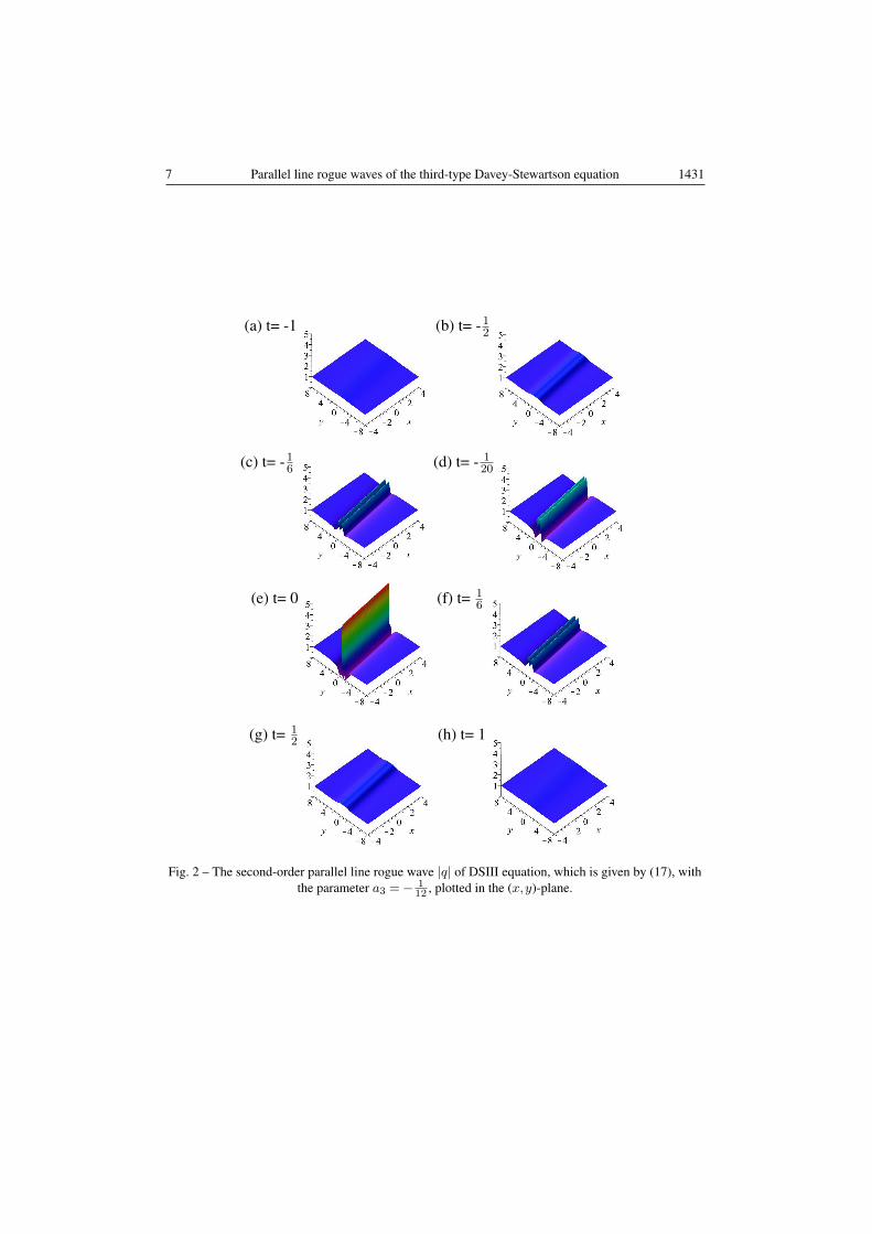
Fig. 3 – The third-order parallel line rogue wave |q| of DSIII equation, which is given by (4), with theparameters in (18), plotted in the (x,y)-plane.

(c) 2016 RRP 68(No. 4) 1425–1446 - v.1.1a*2016.11.24


(a) t= -12 (b) t= -18

(c) t= - 112 (d) t= - 1

20

(e) t= 0 (f) t= 112

(g) t= 18 (h) t= 1

2

Fig. 4 – The fourth-order parallel line rogue wave solution |q| of DSIII equation, which given by (4),with the parameters a3 =−1/12,a5 =−1/240,a7 =−1/4800, plotted in the (x,y)-plane.

(c) 2016 RRP 68(No. 4) 1425–1446 - v.1.1a*2016.11.24


(a) t= -1 (b) t= -12

(c) t= -18 (d) t= - 120

(e) t= 0 (f) t= 18

(g) t= 12 (h) t= 1

Fig. 5 – A fundamental line rogue wave V of DSIII equation, which is given by (15), with theparameter a1 = 0, plotted in the (x,y)-plane.

(c) 2016 RRP 68(No. 4) 1425–1446 - v.1.1a*2016.11.24


(a) t= -1 (b) t= -12

(c) t= - 110 (d) t= - 1

50

(e) t= 0 (f) t= 150

(g) t= 110 (h) t= 1

Fig. 6 – The second-order parallel line rogue wave V of DSIII equation, which is given by (17), withthe parameters a1 = 0, a3 =− 1

12 , plotted in the (x,y)-plane.

(c) 2016 RRP 68(No. 4) 1425–1446 - v.1.1a*2016.11.24


(a) t= -12 (b) t= - 110

(c) t= - 120 (d) t= - 1

100

(e) t= 0 (f) t= 120

(g) t= 110 (h) t= 1

2

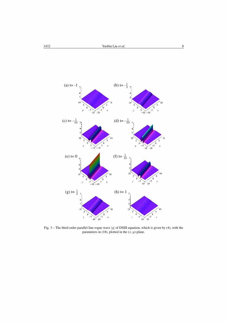
Fig. 7 – The third-order parallel line rogue wave V of DSIII equation, which is given by (4), with theparameters (18), plotted in the (x,y)-plane.

(c) 2016 RRP 68(No. 4) 1425–1446 - v.1.1a*2016.11.24


(a) t= -12 (b) t= - 110

(c) t= - 1100 (d) t= - 1

200

(e) t= 0 (f) t= 1100

(g) t= 110 (h) t= 1

2

Fig. 8 – The fourth-order parallel line rogue wave solution V of DSIII equation, which is given by (4),with the parameters a1 = 0,a3 =−1/12,a5 =−1/240,a7 =−1/4800, plotted in the (x,y)-plane.

(a) (b)

Fig. 9 – The second-order rogue wave V of DSIII equation, which is given by (4), with the papameters(a) a1 = 0, a3 =− 1

12 ,y = 0, and (b) a1 = 0, a3 = 5,y = 0, plotted in the (x,t)-plane.

(c) 2016 RRP 68(No. 4) 1425–1446 - v.1.1a*2016.11.24


(a) (b) (c)

(d) (e) (f)

Fig. 10 – Three patterns of the third-order rogue wave solution V of DSIII equation, which is given by(4), plotted in the (x,t)-plane. (a) The fundamental pattern with parametersa1 = 0,a3 =− 1

12 ,a5 = 0,y = 0. (b) The triangular pattern with parametersa1 = 0,a3 = 20,a5 = 0,y = 0. (c) The ring pattern with parameters a1 = 0,a3 = 0,a5 = 120,y = 0.

The second row provides the corresponding density plots of the first row.

These lines are clearly seen in Fig. 1 (see panel (e)). When t= 0, along the line L1,|q| reaches the maximum amplitude 3 (i.e., three times the height of the background);we call L1 the maximum amplitude line. Along the lines L2 and L3, |q| keeps theminimum amplitude 0, so we call L2 and L3 the minimum amplitude lines. Basedon the above analytical results, we define the direction of the fundamental line roguewave as the direction of the three extreme lines, whose slope is 1

4 . We define thewidth of the line rogue wave as the distance between the two minimum amplitudelines, which is expressed by

Lwidth =2√

17

17

√675t2 + 3.

Furthermore, we define the depth of the line rogue wave as the value of the differencebetween the maximum and minimum amplitudes, which is given by

Ldepth = |q| |L1−|q| |L2

= |q| |L1−|q| |L3

=9

2

√17

675t2 + 3.

Then, it is natural to define the sectional area by the equation

Ssection =1

2Lwidth×Ldepth =

9

2.

These three quantities reflect the local properties of the line rogue wave solution q(see Eq. 15) of the DSIII equation (3).

(c) 2016 RRP 68(No. 4) 1425–1446 - v.1.1a*2016.11.24


(a) (b) (c)

(d)

Fig. 11 – Several patterns of the fourth-order rogue wave solution V of DSIII equation, which is givenby (4), plotted in the (x,t)-plane. (a) The fundamental pattern with parameters

a1 = 0,a3 =− 112 ,a5 =− 1

240 ,a7 =− 14800 ,y = 0. (b) The triangular pattern with parameters

a1 = 0,a3 = 20,a5 = 0,a7 = 0,y = 0. (c) The ring pattern with parametersa1 = 0,a3 =− 1

12 ,a5 =− 1240 ,a7 =− 1

4800 ,y = 0. The inner profile of (c) is a fundamental patternof the second-order rogue wave. (d) The ring pattern with parameters

a1 = 0,a3 =−6,a5 = 6i,a7 = 2000−2i,y = 0. The inner profile of (d) is a triangular pattern of thesecond-order rogue wave.

(a) (b) (c)

(d)

Fig. 12 – The corresponding density plots of the rogue waves shown in Fig. 11.

(c) 2016 RRP 68(No. 4) 1425–1446 - v.1.1a*2016.11.24


(a) (b) (c)

(d)

Fig. 13 – Four rogue wave solutions |A| of the DSI equation in Ref. [12] with ε=−1,N = 1,y = 0,plotted in the (x,t)-plane. (a) The first-order rogue wave solution |A| with parametersn1 = 1, c11 = 0, c10 = 1. (b) The second-order rogue wave solution |A| with parameters

n1 = 2, c12 = 10, c11 = 10, c10 = 1. (c) The third-order rogue wave solution |A| with parametersn1 = 3, c13 = 400+150i,c12 = 0, c11 = 0, c10 = 1. (d) The fourth-order rogue wave solution |A|

with parameters n1 = 4, c14 = 3600+2600i,c13 = 0, c12 = 0, c11 = 0, c10 = 1.

(a) (b) (c)

Fig. 14 – Three rogue wave solutions |q| of DSIII equation, which are given by (4), with y = 0, plottedin the (x,t)-plane. (a) The first-order rogue wave solution |q| with parameter a1 = 0. (b) The

second-order rogue wave solution |q| with parameters a1 = 1,a3 = 4. (c) The third-order rogue wavesolution |q| with parameters a1 = 1,a3 = 3,a5 = 3.

(c) 2016 RRP 68(No. 4) 1425–1446 - v.1.1a*2016.11.24


(a) (b) (c)

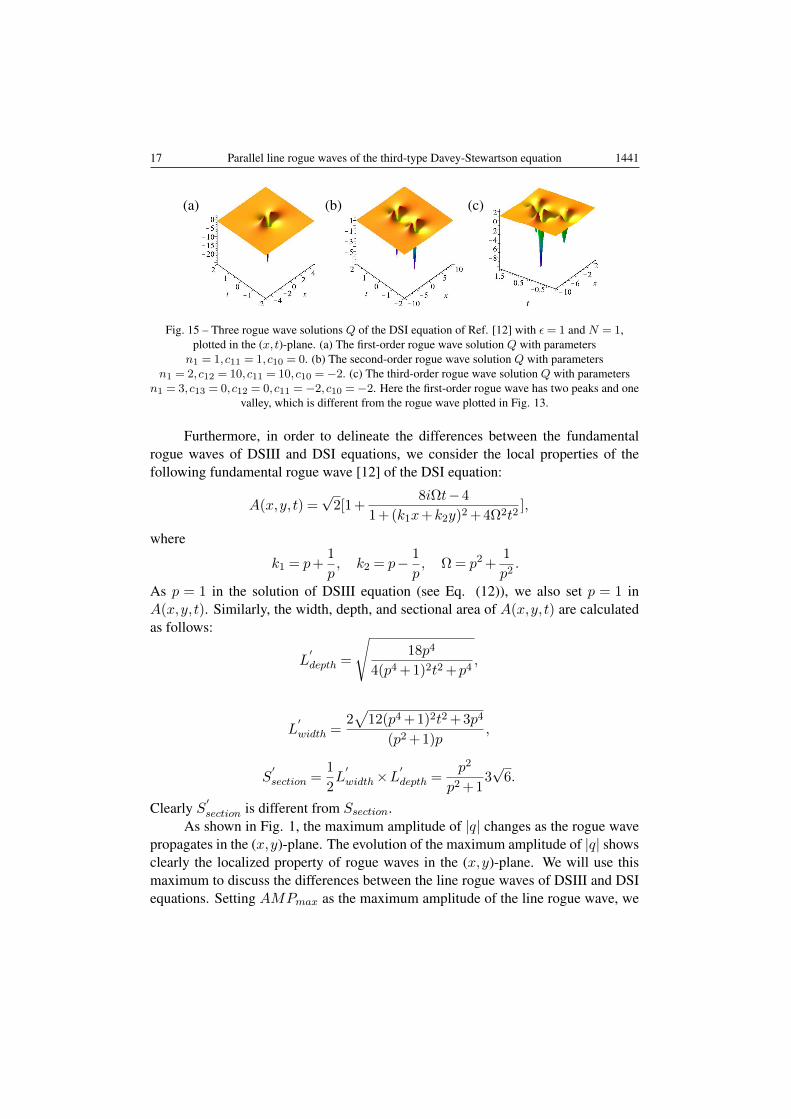
Fig. 15 – Three rogue wave solutions Q of the DSI equation of Ref. [12] with ε= 1 and N = 1,plotted in the (x,t)-plane. (a) The first-order rogue wave solution Q with parametersn1 = 1, c11 = 1, c10 = 0. (b) The second-order rogue wave solution Q with parameters

n1 = 2, c12 = 10, c11 = 10, c10 =−2. (c) The third-order rogue wave solution Q with parametersn1 = 3, c13 = 0, c12 = 0, c11 =−2, c10 =−2. Here the first-order rogue wave has two peaks and one

valley, which is different from the rogue wave plotted in Fig. 13.

Furthermore, in order to delineate the differences between the fundamentalrogue waves of DSIII and DSI equations, we consider the local properties of thefollowing fundamental rogue wave [12] of the DSI equation:

A(x,y, t) =√

2[1 +8iΩt−4

1 + (k1x+k2y)2 + 4Ω2t2],

where

k1 = p+1

p, k2 = p− 1

p, Ω = p2 +

1

p2.

As p = 1 in the solution of DSIII equation (see Eq. (12)), we also set p = 1 inA(x,y, t). Similarly, the width, depth, and sectional area of A(x,y, t) are calculatedas follows:

L′depth =

√18p4

4(p4 + 1)2t2 +p4,

L′width =

2√

12(p4 + 1)2t2 + 3p4

(p2 + 1)p,

S′section =

1

2L′width×L

′depth =

p2

p2 + 13√

6.

Clearly S′section is different from Ssection.

As shown in Fig. 1, the maximum amplitude of |q| changes as the rogue wavepropagates in the (x,y)-plane. The evolution of the maximum amplitude of |q| showsclearly the localized property of rogue waves in the (x,y)-plane. We will use thismaximum to discuss the differences between the line rogue waves of DSIII and DSIequations. Setting AMPmax as the maximum amplitude of the line rogue wave, we

(c) 2016 RRP 68(No. 4) 1425–1446 - v.1.1a*2016.11.24


findAMPmax = |ψ| |L1

= 3

for DSIII equation, and

AMP′max =

√2(16t2 + 9)

16t2 + 1

for DSI equation [12]. Clearly, AMP′max|t=0 =

√2AMPmax. In summary, the

comparison of the above four quantities provides the first difference between therogue waves of DSI and DSIII equations.

The above discussions focused on the fundamental rogue wave solutions ofDSIII equation. We will discuss in the next Section the higher-order rogue wavesolutions corresponding to those given in Theorem 1, for N ≥ 2.

3.3. HIGHER-ORDER ROGUE WAVE SOLUTIONS

For an arbitrary given value of N , we can obtain the N -th order rogue wavesolutions by employing the results of Theorem 1. For example, settingN = 2 in The-orem 1 yields the following explicit form of the second-order rogue wave solutions:

q =

∣∣∣∣∣m(1)11 m

(1)13

m(1)31 m

(1)33

∣∣∣∣∣∣∣∣∣∣m(0)11 m

(0)13

m(0)31 m

(0)33

∣∣∣∣∣,V = (−λlog(

∣∣∣∣∣m(0)11 m

(0)13

m(0)31 m

(1)22

∣∣∣∣∣))yy,U = (−λlog(

∣∣∣∣∣m(0)11 m

(0)13

m(0)31 m

(1)22

∣∣∣∣∣))xx,(17)

where m(n)ij are given in Theorem 1. Setting a0 = 1,a1 = 0, and a2 = 0, the relevant

explicit formulas for the second-order rogue wave solutions involving an arbitraryparameter a3 are given by Eq. (4). Then we obtained very long explicit expressionsfor g(x,y, t) and f(x,y, t) as functions of the variables x, y, and t, which are notgiven here.

The evolution of |q| (see Eq. 17) is plotted in Fig. 2. The maximum of|q(x,y, t,a3)| equals 5 (i.e., five times the height of the background), which is ob-tained at t = 0 with a3 = − 1

12 ; its profile is shown in panel (e) of Fig. 2. It is clearfrom Fig. 2 that this line rogue wave arises from a constant background (see thepanel corresponding to t = −1/2). In subsequent times the two line rogue wavesbegin to interact, and they merge in a single high amplitude line rogue wave with themaximum height attained at t= 0. Unlike the non-fundamental rogue waves of other(2+1)-dimensional soliton equations [12, 13, 15] in which the second-order roguewave has a hyperbola-type shape or a parabola-type shape, here the two straight linerogue waves gradually merge to form a single straight line-shaped rogue wave with

(c) 2016 RRP 68(No. 4) 1425–1446 - v.1.1a*2016.11.24


a large amplitude and furthermore, they preserve the initial direction of the propa-gation. When t > 0, the single line rogue wave gradually splits into two line roguewaves (see Fig. 2 (f)), and finally goes back to the constant background again (seeFig. 2 (h)) at t 0. The parallel lines in the profiles shown in Fig. 2 will be calledparallel line rogue waves [16]. In fact, the other higher-order solutions are also par-allel rogue waves as shown in Figs. 3 and 4.

Now we are in position to consider more complicated cases of Theorem 1, forexample N = 3. In these cases, the higher-order rogue waves have similar profileswith the case of N = 2, but there are now more parallel lines in the rogue wavesarising from the constant background. Then, in subsequent times these line roguewaves interact with each other and create more and more complicated patterns in theinteraction region. For instance, setting N = 3 and considering the parameters

a1 = 0, a3 =− 1

12, a5 =− 1

240(18)

in Theorem 1, we find the third-order parallel line rogue waves shown in Fig. 3.Clearly, the transitional profiles of solution become more convoluted, and the maxi-mum value of solution |q| is 7 (i.e., seven times the height of the background). Thefourth-order parallel line rogue wave |q| is shown in Fig. 4, and there are now fourstraight lines of maximum points in its profile (see the panels (b) and (g) of Fig. 4).As shown in Figs. 3 and 4, the rogue wave solutions |q| are of different form thanthe rogue waves of DSI [12]. The former possess several straight lines, whereas thelatter contain hyperbolic or parabolic curves [12]. Thus, we see the second differencebetween the rogue waves of DSIII and DSI equations: the straight line profiles versusthe curvy profile plotted in Figs. 1, 2, and 3 of Ref. [12].

In addition to |q|, Figs. 5-8 provide the evolution of V , which shows that V is adark rogue wave consisting of several parallel lines. Specifically, we see that a roguewave with very shallow valleys arises from the constant background at early stage(i.e. for t << 0); then, line rogue waves (valleys) start to interact with each other(i.e. as t approaches zero from the left), and then gradually merge to form a deepvalley until the deepest valley is realized at t= 0. Next, the deepest valley graduallysplits as t > 0 into shallow valleys, and finally the rogue waves go back again tothe constant background as t >> 0. The profiles and evolution of V are similar to|q|, excepting the orientation of the extreme lines. Note that the pictures of U aresimilar to V , usually U are also dark rogue waves, but their minimum amplitudes aredifferent.

Like rogue waves of (1+1)-dimensional soliton equations [29–37], the higher-order rogue waves |q|, V , and U of Eq. (3), have three basic patterns, namely thefundamental pattern, the ring pattern, and the triangular pattern. The similaritiesand differences between the profiles of V , U , and |q|, discussed above are similar

(c) 2016 RRP 68(No. 4) 1425–1446 - v.1.1a*2016.11.24


for higher-order rogue waves: the second-order, the third-order, and the fourth-orderrogue wave solutions V are plotted in Figs. 9, 10, 11, and 12. The plot of |q| shownin Fig. 14, is different from the plot of |A| in Fig. 13 for DSI equation. Note that therogue waves V and U have similar profiles, thus we omit to plot the profiles of U .

Motivated by the key features of the rogue waves for the nonlinear Schrodingerequation [32], the obtained results support the following conjectures for the n-thorder rogue waves |q|, V , and U of Eq. (3):(1) For the fundamental pattern where the height of the background is 1, the centralpeak is surrounded by n(n+ 1)−2 gradually decreasing peaks. Note that the heightof the background of V and U is 0.(2) For the triangular and circular patterns, there are n(n+ 1)/2 uniform peaks.(3) For the circular pattern, the n-order rogue wave displays a ring structure, the outerring has 2n− 1 uniform peaks, and the inner structure consists of an (n− 2)-orderrogue wave.

Furthermore, in all the above cases, instead of the multitude of decreasingpeaks, there may exist inner structures of rogue waves, which are composed by first-order and second-order rogue waves. The inner structure of Fig. 10 (c) depicts afirst-order rogue wave, and the inner structure of Fig. 11 (c) depicts a second-orderrogue wave. These inner structures are decomposed from third-order and fourth-order rogue waves, respectively. Thus these plots clearly present two typical exam-ples supporting the conjecture (3).

The n-order rogue wave |A| of the DSI equation can be decomposed into nfirst-order rogue waves (up to third order), and this provides an illustration of thethird difference between the rogue waves of DSI and DSIII equations. We wouldlike to point out that the rogue wave profiles plotted in Fig. 14 are different from therogue wave profiles shown in Fig. 13. For the sake of comparison we plot in Figs. 13and 15 the typical rogue wave solutions of DSI equation according to formulas givenin Ref. [12], for different choices of parameters.

4. SUMMARY AND DISCUSSION

We have derived an explicit formula for the N -th order rogue wave solutionsof the DSIII equation (3) by employing the bilinear transformation method. In or-der to study the properties of the fundamental rogue waves of DSIII equation, wehave defined four quantities, namely Lwidth,Ldepth,Ssection, and AMPmax. Thesequantities characterise the first difference between the rogue waves of DSI and DSIIIequations. The higher-order rogue waves of DSIII equation have several parallelstraight lines in their profiles, and thus they are called parallel line rogue waves; thisprovides the second difference between the rogue waves of DSI and DSIII equations,

(c) 2016 RRP 68(No. 4) 1425–1446 - v.1.1a*2016.11.24


since the rogue waves of DSI equation have curvy profiles. According to Figs. 13and 15, the rogue waves of the DSI equation do not satisfy the conjectures (2) and(3) given in the previous Section; this provides the third difference between the roguewaves of DSI and DSIII equations.

Acknowledgements. This work is supported by the NSF of China under Grant No. 11271210and the K. C. Wong Magna Fund in Ningbo University. Yaobin Liu is supported by the Scientific Re-search Foundation of Graduate School of Ningbo University. A. S. Fokas is supported by EPSRC, UK,via a Senior Fellowship. We thank Mr. Jiguang Rao of Ningbo University for many useful suggestions.

REFERENCES

1. C. Garrett and J. Gemmrich, Phys. Today 62, 62 (2009).2. E. Pelinovsky and C. Kharif, Extreme Ocean Waves, Springer, Berlin, Heidelberg, 2008.3. A. R. Osborne, Nonlinear Ocean Waves and The Inverse Scattering Transform, Academic Press,

New York, 2010.4. D. R. Solli, C. Ropers, P. Koonath, and B. Jalali, Nature 450, 1054 (2007).5. B. Kibler, J. Fatome, C. Finot, G. Millot, F. Dias, G. Genty, N. Akhmediev, and J. M. Dudley,

Nat. Phys. 6, 790 (2010).6. A. Chabchoub, N. P. Hoffmann, and N. Akhmediev, Phys. Rev. Lett. 106, 204502 (2011).7. J. S. He, L. J. Guo, Y. S. Zhang, and A. Chabchoub, Proc. R. Soc. A 470, 20140318 (2014).8. M. Onorato, S. Residori, U. Bortolozzo, A. Montinad, and F. T. Arecchi, Phys. Rep. 528, 47

(2013).9. J. M. Dudley, F. Dias, M. Erkintalo, and G. Genty, Nature Photonics 8, 755 (2014).

10. N. Akhmediev, A. Ankiewicz, and M. Taki, Phys. Lett. A 373, 675 (2009).11. D. Q. Qiu, J. S. He, Y. S. Zhang, and K. Porsezian, Proc. R. Soc. A 471, 20150236 (2015).12. Y. Ohta and J. K. Yang, Phys. Rev. E 86, 036604 (2012).13. Y. Ohta and J. K. Yang, J. Phys. A: Math. Theor. 46, 105202 (2013).14. P. Dubard and V. B. Matveev, Nonlinearity 26, R93 (2013).15. J. C. Chen, Y. Chen, and B. F. Feng, Phys. Lett. A 379, 1510 (2015).16. J. G. Rao, L. H. Wang, Y. Zhang, and J. S. He, Rogue wave solutions of the Zakharov equation,

unpublished.17. D. Q. Qiu, Y. S. Zhang, and J. S. He, Commun. Nonlinear Sci. Numer. Simulat. 30, 307 (2016).18. F. Yuan, J. G. Rao, K. Porsezian, D. Mihalache, and J. S. He, Rom. J. Phys. 61, 378 (2016).19. S. Chen, J. M. Soto-Crespo, F. Baronio, P. Grelu, and D. Mihalache, Opt. Express 24, 15251

(2016).20. M. Boiti, F. Pempinelli, and P. C. Sabatier, Inverse Prob. 9, 1 (1993).21. P. C. Sabatier, Inverse Prob. 8, 263 (1992).22. A. S. Fokas and M. J. Ablowitz, Phys. Rev. Lett. 47, 1096 (1981).23. A. S. Fokas, Inverse Prob. 10, L19 (1994).24. E. I. Schulman, Theor. Math. Phys. 56, 720 (1984).25. P. M. Santini and A. S. Fokas, Commun. Math. Phys. 115, 375 (1988).26. A. S. Fokas and P. M. Santini, Commun. Math. Phys. 116, 499 (1988).27. R. Hirota, The direct method in soliton theory, Cambridge University Press, Cambridge, UK,

2004.

(c) 2016 RRP 68(No. 4) 1425–1446 - v.1.1a*2016.11.24


28. Y. Ohta and J. K. Yang, Proc. R. Soc. A 468, 1716 (2012).29. S. W. Xu, J. S. He, and L. H. Wang, J. Phys. A: Math. Theor. 44, 305203 (2011).30. Y. S. Tao and J. S. He, Phys. Rev. E 85, 026601 (2012).31. S. W. Xu and J. S. He, J. Math. Phys. 53, 063507 (2012).32. J. S. He, H. R. Zhang, L. H. Wang, K. Porsezian, and A. S. Fokas, Phys. Rev. E 87, 052914

(2013).33. J. S. He, L. H. Wang, L. J. Li, K. Porsezian, and R. Erdelyi, Phys. Rev. E 89, 062917 (2014).34. Y. S. Zhang, L. J. Guo, J. S. He, and Z. X. Zhou, Lett. Math. Phys. 105, 853 (2015).35. S. W. Xu, K. Porsezian, J. S. He, and Y. Cheng, Rom. Rep. Phys. 68, 316 (2016).36. D. Mihalache, Rom. Rep. Phys. 67, 1383 (2015).37. S. Chen and D. Mihalache, J. Phys. A: Math. Theor. 48, 215202 (2015).

(c) 2016 RRP 68(No. 4) 1425–1446 - v.1.1a*2016.11.24

Documents

Romanian Reports in Physics, Vol. 68, No. 4, P. 1425–1446 ... · Romanian Reports in Physics, Vol. 68, No. 4, P. 1425–1446, ... eral fundamental rogue waves and which consist