RON: Reverse Connection with Objectness Prior Networks

for Object Detection

Tao Kong1 Fuchun Sun1 Anbang Yao2 Huaping Liu1 Ming Lu3 Yurong Chen2

1State Key Lab. of Intelligent Technology and Systems, Tsinghua National Laboratory for

Information Science and Technology (TNList), Department of Computer Science and Technology,

Tsinghua University 2Intel Labs China 3Department of Electronic Engineering, Tsinghua University1{kt14@mails,fcsun@,hpliu@}.tsinghua.edu.cn

2{anbang.yao, yurong.chen}@.intel.com 3lu-m13@mails.tsinghua.edu.cn

Abstract

We present RON, an efficient and effective framework for

generic object detection. Our motivation is to smartly as-

sociate the best of the region-based (e.g., Faster R-CNN)

and region-free (e.g., SSD) methodologies. Under fully con-

volutional architecture, RON mainly focuses on two funda-

mental problems: (a) multi-scale object localization and (b)

negative sample mining. To address (a), we design the re-

verse connection, which enables the network to detect ob-

jects on multi-levels of CNNs. To deal with (b), we propose

the objectness prior to significantly reduce the searching s-

pace of objects. We optimize the reverse connection, object-

ness prior and object detector jointly by a multi-task loss

function, thus RON can directly predict final detection re-

sults from all locations of various feature maps.

Extensive experiments on the challenging PASCAL VOC

2007, PASCAL VOC 2012 and MS COCO benchmarks

demonstrate the competitive performance of RON. Specifi-

cally, with VGG-16 and low resolution 384×384 input size,

the network gets 81.3% mAP on PASCAL VOC 2007, 80.7%

mAP on PASCAL VOC 2012 datasets. Its superiority in-

creases when datasets become larger and more difficult, as

demonstrated by the results on the MS COCO dataset. With

1.5G GPU memory at test phase, the speed of the network

is 15 FPS, 3× faster than the Faster R-CNN counterpart.

Code will be made publicly available.

1. Introduction

We are witnessing significant advances in object detec-

tion area, mainly thanks to the deep networks. Current top

deep-networks-based object detection frameworks could be

grouped into two main streams: the region-based methods

[11][23][10][16] and the region-free methods [22][19].

The region-based methods divide the object detection

(a) (b) (c) (d)

Figure 1. Objectness prior generated from a specific image. In this

example, sofa is responded at scales (a) and (b), the brown dog

is responded at scale (c) and the white spotted dog is responded

at scale (d). The network will generate detection results with the

guidance of objectness prior .

task into two sub-problems: At the first stage, a dedicat-

ed region proposal generation network is grafted on deep

convolutional neural networks (CNNs) which could gen-

erate high quality candidate boxes. Then at the second

stage, a region-wise subnetwork is designed to classify

and refine these candidate boxes. Using very deep C-

NNs [14][27], the Fast R-CNN pipeline [10][23] has re-

cently shown high accuracy on mainstream object detection

benchmarks [7][24][18]. The region proposal stage could

reject most of the background samples, thus the searching

space for object detection is largely reduced [1][32]. Multi-

stage training process is usually developed for joint opti-

mization of region proposal generation and post detection

(e.g., [4][23][16]). In Fast R-CNN [10], the region-wise

subnetwork repeatedly evaluates thousands of region pro-

posals to generate detection scores. Under Fast R-CNN

pipeline, Faster R-CNN shares full-image convolutional

features with the detection network to enable nearly cost-

free region proposals. Recently, R-FCN [4] tries to make

the unshared per-RoI computation of Faster R-CNN to be

sharable by adding position-sensitive score maps. Never-

theless, R-FCN still needs region proposals generated from

region proposal networks [23]. To ensure detection accura-

cy, all methods resize the image to a large enough size (usu-

15936

ally with the shortest side of 600 pixels). It is somewhat

resource/time consuming when feeding the image into deep

networks, both in training and inference time. For example,

predicting with Faster R-CNN usually takes 0.2 ms per im-

age using about 5GB GPU memory for VGG-16 networks

[27].

Another solution family is the region-free methods

[22][19]. These methods treat object detection as a single

shot problem, straight from image pixels to bounding box

coordinates by fully convolutional networks (FCNs). The

main advantage of these detectors is high efficiency. Origi-

nated from YOLO [22], SSD [19] tries to deal object detec-

tion problem with multiple layers of deep CNNs. With low

resolution input, the SSD detector could get state-of-the-art

detection results. However, the detection accuracy of these

methods still has room for improvement: (a) Without region

proposals, the detectors have to suppress all of the negative

candidate boxes only at the detection module. It will in-

crease the difficulties on training the detection module. (b)

YOLO detects objects with the top-most CNN layer, with-

out deeply exploring the detection capacities of different

layers. SSD tries to improve the detection performance by

adding former layers’ results. However, SSD still struggles

with small instances, mainly because of the limited infor-

mation of middle layers. These two main bottlenecks affect

the detection accuracy of the methods.

Driven by the success of the two solution families, a

critical question arises: is it possible to develop an ele-

gant framework which can smartly associate the best of

both methodologies and eliminate their major demerits?

We answer this question by trying to bridge the gap be-

tween the region-based and region-free methodologies. To

achieve this goal, we focus on two fundamental problem-

s: (a) Multi-scale object localization. Objects of various

scales could appear at any position of an image, so tens of

thousands of regions with different positions/scales/aspect

ratios should be considered. Prior works [16][3] show that

multi-scale representation will significantly improve object

detection of various scales. However, these methods always

detect various scales of objects at one layer of a network

[16][23][4]. With the proposed reverse connection, objects

are detected on their corresponding network scales, which

is more elegant and easier to optimize. (b) Negative space

mining. The ratio between object and non-object samples

is seriously imbalanced. So an object detector should have

effective negative mining strategies [26]. In order to reduce

the searching space of the objects, we create an objectness

prior (Figure 1) on convolutional feature maps and jointly

optimize it with the detector at training phase.

As a result, we propose RON (Reverse connection

with Objectness prior Networks) object detection frame-

work, which could associate the merits of region-based and

region-free approaches. Furthermore, recent complemen-

tary advances such as hard example mining [26], bounding

box regression [11] and multi-layer representation [16][3]

could be naturally employed.

Contributions. We make the following contributions:

1. We propose RON, a fully convolutional framework for

end-to-end object detection. Firstly, the reverse con-

nection assists the former layers of CNNs with more

semantic information. Second, the objectness prior

gives an explicit guide to the searching of objects. Fi-

nally, the multi-task loss function enables us to opti-

mize the whole network end-to-end on detection per-

formance.

2. In order to achieve high detection accuracy, effective

training strategies like negative example mining and

data augmentation have been employed. With low res-

olution 384×384 input size, RON achieves state-of-

the-art results on PASCAL VOC 2007, with a 81.3%

mAP, VOC 2012, with a 80.7% mAP, and MS COCO,

with a 27.4% mAP.

3. RON is time and resource efficient. With 1.5G GPU

memory, the total feed-forward speed is 15 FPS, 3×faster than the seminal Faster R-CNN. Moreover, we

conduct extensive design choices like the layers com-

bination, with/without objectness prior, and other vari-

ations.

2. Related Work

Object detection is a fundamental and heavily-

researched task in computer vision area. It aims to local-

ize and recognize every object instance with a bounding

box [7][18]. Before the success of deep CNNs [17], the

widely used detection systems are based on the combina-

tion of independent components (HOG [30], SIFT [21] et

al.). The DPM [8] and its variants [2][5] have been the dom-

inant methods for years. These methods use object compo-

nent descriptors as features and sweep through the entire

image to find regions with a class-specific maximum re-

sponse. With the great success of the deep learning on large

scale object recognition, several works based on CNNs have

been proposed [31][25]. R-CNN [11] and its variants usu-

ally combine region proposals (generated from Selective

Search [29], Edgeboxes [32], MCG [1], et al.) and ConvNet

based post-classification. These methods have brought dra-

matic improvement on detection accuracy [17]. After the

original R-CNN, researches are improving it in a variety of

ways. The SPP-Net [13] and Fast R-CNN [10] speed up

the R-CNN approach with RoI-Pooling (Spatial-Pyramid-

Pooling) that allows the classification layers to reuse fea-

tures computed over CNN feature maps. Under Fast R-

CNN pipeline, several works try to improve the detection

speed and accuracy, with more effective region proposals

5937

conv4

......

...

conv5 conv6 conv7

reverse

connection

det 7

det 6

det 5

det 4

objectness

objectnessobjectness

objectness

reverse

connection

reverse

connection

boat

boatperson

Figure 2. RON object detection overview. Given an input image,

the network firstly computes features of the backbone network.

Then at each detection scale: (a) adds reverse connection; (b) gen-

erates objectness prior; (c) detects object on its corresponding CN-

N scales and locations. Finally, all detection results are fused and

selected with non-maximum suppression.

[23], multi-layer fusion [3][16], context information [14][9]

and more effective training strategy [26]. R-FCN [4] tries

to reduce the computation time with position-sensitive score

maps under ResNet architecture [14]. Thanks to the FCN-

s [20] which could give position-wise information of input

images, several works are trying to solve the object detec-

tion problem by FCNs. The methods skip the region propos-

al generation step and predict bounding boxes and detection

confidences of multiple categories directly [6]. YOLO [22]

uses the top most CNN feature maps to predict both con-

fidences and locations for multiple categories. Originated

from YOLO, SSD [19] tries to predict detection results at

multiple CNN layers. With carefully designed training s-

trategies, SSD could get competitive detection results. The

main advantage of these methods is high time-efficiency.

For example, the feed-forward speed of YOLO is 45 FPS,

9× faster than Faster R-CNN.

3. Network Architecture

This section describes RON object detection framework

(Figure 2). We first introduce the reverse connection on tra-

ditional CNNs in Section 3.1, such that different network

scales have effective detection capabilities. Then in Section

3.2, we explain how to generate candidate boxes on differ-

ent network scales. Next, we present the objectness prior

to guide the search of objects in Section 3.3 and Secction

3.4. Finally, we combine the objectness prior and object de-

tection into a unified network for joint training and testing

(Section 3.5).

Network preparation We use VGG-16 as the test

case reference model, which is pre-trained with ImageNet

dataset [27]. Recall that VGG-16 has 13 convolutional lay-

conv n

deconv

2×2, 512

conv

3×3, 512

sum

rf-map n+1

rf-map n

Figure 3. A reverse connection block.

ers and 3 fully-connected layers. We convert FC6 (14th lay-

er) and FC7 (15th layer) to convolutional layers [20], and

use 2×2 convolutional kernels with stride 2 to reduce the

resolution of FC7 by half1. By now, the feature map sizes

used for object detection are 1/8 (conv 4 3), 1/16 (con-

v 5 3), 1/32 (conv 6) and 1/64 (conv 7) of the input size,

both in width and height (see Figure 2 top).

3.1. Reverse Connection

Combining fine-grained details with highly-abstracted

information helps object detection with different scales

[12][20][14]. The region-based networks usually fuse mul-

tiple CNN layers into a single feature map [3][16]. Then ob-

ject detection is performed on the fused maps with region-

wise subnetworks [10]. As all objects need to be detected

based on the fixed features, the optimization becomes much

complex. SSD [19] detects objects on multiple CNN layers.

However, the semantic information of former layers is limit-

ed, which affects the detection performance of these layers.

This is the reason why SSD has much worse performance

on smaller objects than bigger objects [19].

Inspired from the success of residual connection [14]

which eases the training of much deeper networks, we pro-

pose the reverse connection on traditional CNN architec-

tures. The reverse connection enables former features to

have more semantic information. One reverse connection

block is shown in Figure 3. Firstly, a deconvolutional layer

is applied to the reverse fusion map (annotated as rf-map)

n+1, and a convolutional layer is grafted on backbone lay-

er n to guarantee the inputs have the same dimension. Then

the two corresponding maps are merged by element-wise

addition. The reverse fusion map 7 is the convolutional out-

put (with 512 channels by 3×3 kernels) of the backbone

layer 7. After this layer has been generated, each reverse

connection block will be generated in the same way, as

shown in Figure 2. In total, there are four reverse fusion

maps with different scales.

Compared with methods using single layer for objec-

t detection [16][23], multi-scale representation is more ef-

fective on locating all scales of objects (as shown in ex-

periments). More importantly, as the reverse connection is

learnable, the semantic information of former layers can be

1The last FC layer (16th layer) is not used in this paper.

5938

significantly enriched. This characteristic makes RON more

effective in detecting all scales of objects compared with

[19].

3.2. Reference Boxes

In this section, we describe how to generate bounding

boxes on feature maps produced from Section 3.1. Feature

maps from different levels within a network are known to

have different receptive field sizes [13]. As the reverse con-

nection can generate multiple feature maps with different

scales. We can design the distribution of boxes so that spe-

cific feature map locations can be learned to be responsive

to particular scales of objects. Denoting the minimum scale

with smin, the scales Sk of boxes at each feature map k are

Sk = {(2k − 1) · smin, 2k · smin}, k ∈ {1, 2, 3, 4}. (1)

We also impose different aspect ratios { 1

3, 1

2, 1, 2, 3} for the

default boxes. The width and height of each box are com-

puted with respect to the aspect ratio [23]. In total, there

are 2 scales and 5 aspect ratios at each feature map loca-

tion. The smin is 1

10of the input size (e.g., 32 pixels for

320×320 model). By combining predictions for all default

boxes with different scales and aspect ratios, we have a di-

verse set of predictions, covering various object sizes and

shapes.

3.3. Objectness Prior

As shown in Section 3.2, we consider default boxes with

different scales and aspect ratios from many feature map-

s. However, only a tiny fraction of boxes covers object-

s. In other words, the ratio between object and non-object

samples is seriously imbalanced. The region-based meth-

ods overcome this problem by region proposal networks

[16][23]. However, the region proposals will bring trans-

lation variance compared with the default boxes. So the

Fast R-CNN pipeline usually uses region-wise networks for

post detection, which brings repeated computation [4]. In

contrast, we add an objectness prior for guiding the search

of objects, without generating new region proposals. Con-

cretely, we add a 3×3×2 convolutional layer followed by

a Softmax function to indicate the existence of an object in

each box. The channel number of objectness prior maps is

10, as there are 10 default boxes at each location.

Figure 1 shows the multi-scale objectness prior generat-

ed from a specific image. For visualization, the objectness

prior maps are averaged along the channel dimension. We

see that the objectness prior maps could explicitly reflec-

t the existence of an object. Thus the searching space of

the objects could be dramatically reduced. Objects of vari-

ous scales will respond at their corresponding feature maps,

and we enable this by appropriate matching and end-to-end

training. More results could be seen in the experiment sec-

tion.

conv

3×3, 512

concat

former layer

conv

1×1, 512

latter layer

Figure 4. One inception block.

3.4. Detection and Bounding Box Regression

Different from objectness prior, the detection module

needs to classify regions into K+1 categories (K= 20 for

PASCAL VOC dataset and K= 80 for MS COCO dataset,

plus 1 for background). We employ the inception module

[28] on the feature maps generated in Section 3.1 to per-

form detection. Concretely, we add two inception blocks

(one block is shown in Figure 4) on feature maps, and clas-

sify the final inception outputs. There are many inception

choices as shown in [28]. In this paper, we just use the most

simple structure.

With Softmax, the sub-network outputs the per-class s-

core that indicates the presence of a class-specific instance.

For bounding box regression, we predict the offsets relative

to the default boxes in the cell (see Figure 5).

rf-map n softmax

bbox reg

conv

3×3, (k+1)×A

inception

conv

3×3, 4×A

conv

3×3, 512

inception

Figure 5. Object detection and bounding box regression modules.

Top: bounding box regression; Bottom: object classification.

3.5. Combining Objectness Prior with Detection

In this section, we explain how RON combines object-

ness prior with object detection. We assist object detection

with objectness prior both in training and testing phases.

For training the network, we firstly assign a binary class

label to each candidate region generated from Section 3.2.

Then if the region covers object, we also assign a class-

specific label to it. For each ground truth box, we (i) match

it with the candidate region with most jaccard overlap; (ii)

match candidate regions to any ground truth with jaccard

overlap higher than 0.5. This matching strategy guarantees

that each ground truth box has at least one region box as-

signed to it. We assign negative labels to the boxes with

jaccard overlap lower than 0.3.

By now, each box has its objectness label and class-

specific label. The network will update the class-specific

labels dynamically for assisting object detection with ob-

jectness prior at training phase. For each mini-batch at feed-

5939

forward time, the network runs both the objectness prior and

class-specific detection. But at the back-propagation phase,

the network firstly generates the objectness prior, then for

detection, samples whose objectness scores are high than

threshold op are selected (Figure 6). The extra computa-

tion only comes from the selection of samples for back-

propagation. With suitable op (we use op = 0.03 for al-

l models), only a small number of samples is selected for

updating the detection branch, thus the complexity of back-

ward pass has been significantly reduced.

Figure 6. Mapping the objectness prior with object detection. We

first binarize the objectness prior maps according to op, then

project the binary masks to the detection domain of the last convo-

lutional feature maps. The locations within the masks are collected

for detecting objects.

4. Training and Testing

In this section, we firstly introduce the multi-task loss

function for optimizing the networks. Then we explain how

to optimize the network jointly and perform inference di-

rectly.

4.1. Loss Function

For each location, our network has three sibling output

branches. The first outputs the objectness confidence score

pobj = {pobj0

, pobj1

}, computed by a Softmax over the 2×Aoutputs of objectness prior (A = 10 in this paper, as there

are 10 types of default boxes). We denote the objectness

loss with Lobj . The second branch outputs the bounding-

box regression loss, denoted by Lloc. It targets at mini-

mizing the smoothed L1 loss [10] between the predicted

location offsets t = (tx, ty, tw, th) and the target offset-

s t∗ = (t∗x, t∗y, t

∗w, t

∗h). Different from Fast R-CNN [10]

that regresses the offsets for each of K classes, we just

regress the location one time with no class-specific informa-

tion. The third branch outputs the classification loss Lcls|obj

for each box, over K+1 categories. Given the object-

ness confidence score pobj , the branch first excludes region-

s whose scores are lower than the threshold op. Then like

Lobj , Lcls|obj is computed by a Softmax over K+1 outputs

for each location pcls|obj = {pcls|obj0

, pcls|obj1

, . . . , pcls|objK }.

We use a multi-task loss L to jointly train the networks end-

to-end for objectness prior, classification and bounding-box

regression:

L = α1

Nobj

Lobj+β1

Nloc

Lloc+(1−α−β)1

Ncls|objLcls|obj .

(2)

The hyper-parameters α and β in Equation 2 control the

balance between the three losses. We normalize each loss

term with its input number. Under this normalization, α =β = 1

3works well and is used in all experiments.

4.2. Joint Training and Testing

We optimize the models described above jointly with

end-to-end training. After the matching step, most of the

default boxes are negatives, especially when the number of

default boxes is large. Here, we introduce a dynamic train-

ing strategy to scan the negative space. At training phase,

each SGD mini-batch is constructed from N images cho-

sen uniformly from the dataset. At each mini-batch, (a) for

objectness prior, all of the positive samples are selected for

training. Negative samples are randomly selected from re-

gions with negative labels such that the ratio between pos-

itive and negative samples is 1:3; (b) for detection, we first

reduce the sample number according to objectness prior s-

cores generated at this mini-batch (as discribed in Section

3.5). Then all of the positive samples are selected. We ran-

domly select negative samples such that the ratio between

positive and negative samples is 1:3. We note that recent

works such as Faster R-CNN [23] and R-FCN [4] usually

use multi-stage training for joint optimization. In contrast,

the loss function 2 is trained end-to-end in our implemen-

tation by back-propagation and SGD, which is more effi-

cient at training phase. At the beginning of training, the

objectness prior maps are in chaos. However, along with

the training progress, the objectness prior maps are more

concentrated on areas covering objects.

Data augmentation To make the model more robust to

various object scales, each training image is randomly sam-

pled by one of the following options: (i) Using the orig-

inal/flipped input image; (ii) Randomly sampling a patch

whose edge length is { 4

10, 5

10, 6

10, 7

10, 8

10, 9

10} of the origi-

nal image and making sure that at least one object’s center

is within this patch. We note that the data augmentation

strategy described above will increase the number of large

objects, but the optimization benefit for small objects is lim-

ited. We overcome this problem by adding a small scale for

training. A large object at one scale will be smaller at s-

maller scales. This training strategy could effectively avoid

over-fitting of objects with specific sizes.

Inference At inference phase, we multiply the class-

conditional probability and the individual box confidence

5940

Method mAP aero bike bird boat bottle bus car cat chair cow table dog horse mbike person plant sheep sofa train tv

Fast R-CNN[10] 70.0 77.0 78.1 69.3 59.4 38.3 81.6 78.6 86.7 42.8 78.8 68.9 84.7 82.0 76.6 69.9 31.8 70.1 74.8 80.4 70.4

Faster R-CNN[23] 73.2 76.5 79.0 70.9 65.5 52.1 83.1 84.7 86.4 52.0 81.9 65.7 84.8 84.6 77.5 76.7 38.8 73.6 73.9 83.0 72.6

SSD300[19] 72.1 75.2 79.8 70.5 62.5 41.3 81.1 80.8 86.4 51.5 74.3 72.3 83.5 84.6 80.6 74.5 46.0 71.4 73.8 83.0 69.1

SSD500[19] 75.1 79.8 79.5 74.5 63.4 51.9 84.9 85.6 87.2 56.6 80.1 70.0 85.4 84.9 80.9 78.2 49.0 78.4 72.4 84.6 75.5

RON320 74.2 75.7 79.4 74.8 66.1 53.2 83.7 83.6 85.8 55.8 79.5 69.5 84.5 81.7 83.1 76.1 49.2 73.8 75.2 80.3 72.5

RON384 75.4 78.0 82.4 76.7 67.1 56.9 85.3 84.3 86.1 55.5 80.6 71.4 84.7 84.8 82.4 76.2 47.9 75.3 74.1 83.8 74.5

RON320++ 76.6 79.4 84.3 75.5 69.5 56.9 83.7 84.0 87.4 57.9 81.3 74.1 84.1 85.3 83.5 77.8 49.2 76.7 77.3 86.7 77.2

RON384++ 77.6 86.0 82.5 76.9 69.1 59.2 86.2 85.5 87.2 59.9 81.4 73.3 85.9 86.8 82.2 79.6 52.4 78.2 76.0 86.2 78.0

Table 1. Detection results on PASCAL VOC 2007 test set. The entries with the best APs for each object category are bold-faced.

Figure 7. Visualization of performance for RON384 on animals, vehicles, and furniture from VOC2007 test. The Figures show the

cumulative fraction of detections that are correct (Cor) or false positive due to poor localization (Loc), confusion with similar categories

(Sim), with others (Oth), or with background (BG). The solid red line reflects the change of recall with the ‘strong’ criteria (0.5 jaccard

overlap) as the number of detections increases. The dashed red line uses the ‘weak’ criteria (0.1 jaccard overlap).

predictions. The class-specific confidence score for each

box is defined as Equation 3:

pcls = pobj · pcls|obj . (3)

The scores encode both the probability of the class appear-

ing in the box and how well the predicted box fits the object.

After the final score of each box is generated, we adjust the

boxes according to the bounding box regression outputs. Fi-

nally, non-maximum suppression is applied to get the final

detection results.

5. Results

We train and evaluate our models on three major dataset-

s: PASCAL VOC 2007, PASCAL VOC 2012, and MS CO-

CO. For fair comparison, all experiments are based on the

VGG-16 networks. We train all our models on a single N-

vidia TitanX GPU, and demonstrate state-of-the-art results

on all three datasets.

5.1. PASCAL VOC 2007

On this dataset, we compare RON against seminal Fast

R-CNN [10], Faster R-CNN [23], and the most recently

proposed SSD [19]. All methods are trained on VOC2007

trainval and VOC2012 trainval, and tested on VOC2007 test

dataset. During training phase, we initialize the parameter-

s for all the newly added layers by drawing weights from

a zero-mean Gaussian distribution with standard deviation

0.01. All other layers are initialized by standard VGG-16

model [10]. We use the 10−3 learning rate for the first 90k

iterations, then we decay it to 10−4 and continue training

for next 30k iterations. The batch size is 18 for 320×320model according to the GPU capacity. We use a momentum

of 0.9 and a weight decay of 0.0005.

Table 1 shows the result comparisons of the methods2.

With 320×320 input size, RON is already better than Faster

R-CNN. By increasing the input size to 384×384, RON

gets 75.4% mAP, outperforming Faster R-CNN by a mar-

gin of 2.2%. RON384 is also better than SSD with input

size 500×500. Finally, RON could achieve high mAPs of

76.6% (RON320++) and 77.6% (RON384++) with multi-

scale testing, bounding box voting and flipping [3].

Small objects are challenging for detectors. As shown

in Table 1, all methods have inferior performance on ‘boat’

and ‘bottle’. However, RON improves performance of these

categories by significant margins: 4.0 points improvement

for ‘boat’ and 7.1 points improvement for ‘bottle’. In sum-

mary, performance of 17 out of 20 categories has been im-

proved by RON.

To understand the performance of RON in more detail,

we use the detection analysis tool from [15]. Figure 7 shows

that our model can detect various object categories with

2We note that the latest SSD uses new training tricks (color distortion,

random expansion and online hard example mining), which makes the re-

sults much better. We expect these tricks will also improve our results,

which is beyond the focus of this paper.

5941

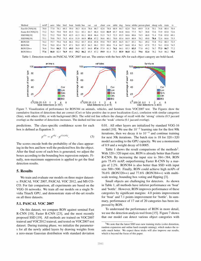
Method mAP aero bike bird boat bottle bus car cat chair cow table dog horse mbike person plant sheep sofa train tv

Fast R-CNN[10] 68.4 82.3 78.4 70.8 52.3 38.7 77.8 71.6 89.3 44.2 73.0 55.0 87.5 80.5 80.8 72.0 35.1 68.3 65.7 80.4 64.2

OHEM[26] 71.9 83.0 81.3 72.5 55.6 49.0 78.9 74.7 89.5 52.3 75.0 61.0 87.9 80.9 82.4 76.3 47.1 72.5 67.3 80.6 71.2

Faster R-CNN[23] 70.4 84.9 79.8 74.3 53.9 49.8 77.5 75.9 88.5 45.6 77.1 55.3 86.9 81.7 80.9 79.6 40.1 72.6 60.9 81.2 61.5

HyperNet[16] 71.4 84.2 78.5 73.6 55.6 53.7 78.7 79.8 87.7 49.6 74.9 52.1 86.0 81.7 83.3 81.8 48.6 73.5 59.4 79.9 65.7

SSD300[19] 70.3 84.2 76.3 69.6 53.2 40.8 78.5 73.6 88.0 50.5 73.5 61.7 85.8 80.6 81.2 77.5 44.3 73.2 66.7 81.1 65.8

SSD500[19] 73.1 84.9 82.6 74.4 55.8 50.0 80.3 78.9 88.8 53.7 76.8 59.4 87.6 83.7 82.6 81.4 47.2 75.5 65.6 84.3 68.1

RON320 71.7 84.1 78.1 71.0 56.8 46.9 79.0 74.7 87.5 52.5 75.9 60.2 84.8 79.9 82.9 78.6 47.0 75.7 66.9 82.6 68.4

RON384 73.0 85.4 80.6 71.9 56.3 49.8 80.6 76.8 88.2 53.6 78.1 60.4 86.4 81.5 83.8 79.4 48.6 77.4 67.7 83.4 69.5

RON320++ 74.5 87.1 81.0 74.6 58.8 51.7 82.1 77.0 89.7 57.2 79.9 62.6 87.2 83.2 85.0 80.5 51.4 76.7 68.5 84.8 70.4

RON384++ 75.4 86.5 82.9 76.6 60.9 55.8 81.7 80.2 91.1 57.3 81.1 60.4 87.2 84.8 84.9 81.7 51.9 79.1 68.6 84.1 70.3

Table 2. Results on PASCAL VOC 2012 test set. All methods are based on the pre-trained VGG-16 networks.

high quality. The recall is higher than 85%, and is much

higher with the ‘weak’ (0.1 jaccard overlap) criteria.

5.2. PASCAL VOC 2012

We compare RON against top methods on the comp4

(outside data) track from the public leaderboard on PAS-

CAL VOC 2012. The training data is the union set of all

VOC 2007, VOC 2012 train and validation datasets, fol-

lowing [23][10][19]. We see the same performance trend as

we observed on VOC 2007 test. The results, as shown in

Table 2, demonstrate that our model performs the best on

this dataset. Compared with Faster R-CNN and other vari-

ants [26][16], the proposed network is significantly better,

mainly due to the reverse connection and the use of boxes

from multiple feature maps.

5.3. MS COCO

To further validate the proposed framework on a larger

and more challenging dataset, we conduct experiments on

MS COCO [18] and report results from test-dev2015 evalu-

ation server. The evaluation metric of MS COCO dataset is

different from PASCAL VOC. The average mAP over dif-

ferent IoU thresholds, from 0.5 to 0.95 (written as 0.5:0.95)

is the overall performance of methods. This places a sig-

nificantly larger emphasis on localization compared to the

PASCAL VOC metric which only requires IoU of 0.5. We

use the 80k training images and 40k validation images [23]

to train our model, and validate the performance on the test-

dev2015 dataset which contains 20k images. We use the

5×10−4 learning rate for 400k iterations, then we decay

it to 5×10−5 and continue training for another 150k itera-

tions. As instances in MS COCO dataset are smaller and

denser than those in PASCAL VOC dataset, the minimum

scale smin of the referenced box size is 24 for 320×320

model, and 32 for 384×384 model. Other settings are the

same as PASCAL VOC dataset.

With the standard COCO evaluation metric, Faster R-

CNN scores 21.9% AP, and RON improves it to 27.4% AP.

Using the VOC overlap metric of IoU ≥0.5, RON384++

gives a 5.8 points boost compared with SSD500. It is also

interesting to note that with 320×320 input size, RON gets

Method Train DataAverage Precision

0.5 0.75 0.5:0.95

Fast R-CNN[10] train 35.9 - 19.7

OHEM[26] trainval 42.5 22.2 22.6

OHEM++[26] trainval 45.9 26.1 25.5

Faster R-CNN[23] trainval 42.7 - 21.9

SSD300[19] trainval35k 38.0 20.5 20.8

SSD500[19] trainval35k 43.7 24.7 24.4

RON320 trainval 44.7 22.7 23.6

RON384 trainval 46.5 25.0 25.4

RON320++ trainval 47.5 25.9 26.2

RON384++ trainval 49.5 27.1 27.4

Table 3. MS COCO test-dev2015 detection results.

26.2% AP, improving the SSD with 500×500 input size by

1.8 points on the strict COCO AP evaluation metric.

We also compare our method against Fast R-CNN with

online hard example mining (OHEM) [26], which gives

a considerable improvement on Fast R-CNN. The OHEM

method also adopts recent bells and whistles to further im-

prove the detection performance. The best result of OHEM

is 25.5% AP (OHEM++). RON gets 27.4% AP, which

demonstrates that the proposed network is more competi-

tive on large dataset.

5.4. From MS COCO to PASCAL VOC

Large-scale dataset is important for improving deep neu-

ral networks. In this experiment, we investigate how the

MS COCO dataset can help with the detection performance

of PASCAL VOC. As the categories on MS COCO are a

superset of these on PASCAL VOC dataset, the fine-tuning

process becomes easier compared with the ImageNet pre-

trained model. Starting from MS COCO pre-trained mod-

el, RON leads to 81.3% mAP on PASCAL VOC 2007 and

80.7% mAP on PASCAL VOC 2012.

The extra data from the MS COCO dataset increases

the mAP by 3.7% and 5.3%. Table 4 shows that the mod-

el trained on COCO+VOC has the best mAP on PASCAL

VOC 2007 and PASCAL VOC 2012. When submitting, our

model with 384×384 input size has been ranked as the top 1

on the VOC 2012 leaderboard among VGG-16 based mod-

els. We note that other public methods with better results

are all based on much deeper networks [14].

5942

Method 2007 test 2012 test

Faster R-CNN[23] 78.8 75.9

OHEM++[26] - 80.1

SSD512[19] - 80.0

RON320 78.7 76.3

RON384 80.2 79.0

RON320++ 80.3 78.7

RON384++ 81.3 80.7

Table 4. The performance on PASCAL VOC datasets. All models

are pre-trained on MS COCO, and fine-tuned on PASCAL VOC.

6. Ablation Analysis

6.1. Do Multiple Layers Help?

As described in Section 3, our networks generate detec-

tion boxes from multiple layers and combine the results. In

this experiment, we compare how layer combinations affect

the final performance. For all of the following experiments

as shown in Table 5, we use exactly the same settings and

input size (320×320), except for the layers for object detec-

tion.

detection from layermAP

4 5 6 7

X 65.6

X X 68.3

X X X 72.5

X X X X 74.2

Table 5. Combining features from different layers.

From Table 5, we see that it is necessary to use all of the

layer 4, 5, 6 and 7 such that the detector could get the best

performance.

6.2. Objectness Prior

As introduced in Section 3.3, the network generates ob-

jectness prior for post detection. The objectness prior maps

involve not only the strength of the responses, but also their

spatial positions. As shown in Figure 8, objects with various

scales will respond at the corresponding maps. The map-

s can guide the search of different scales of objects, thus

significantly reducing the searching space.

input map4 map5 map6 map7

Figure 8. Objectness prior maps generated from images.

We also design an experiment to verify the effect of ob-

jectness prior. In this experiment, we remove the objectness

prior module and predict the detection results only from the

detection module. Other settings are exactly the same as the

baseline. Removing objectness prior maps leads to 69.6%

mAP on VOC 2007 test dataset, resulting 4.6 points drop

from the 74.2% mAP baseline.

6.3. Generating Region Proposals

After removing the detection module, our network could

get region proposals. We compare the proposal perfor-

mance against Faster R-CNN [23] and evaluate recalls with

different numbers of proposals on PASCAL VOC 2007 test

set, as shown in Figure 9.

✶ ✶� ✶�� ✶����

�✵✁

�✵✂

�✵✄

�✵☎

✶

♥✆✝✞✟✠ ✡☛ ☞✠✡☞✡✌✍✎✌

r✏✑✒✓✓

❖✆✠✌

❋✍✌✔✟✠ ✕✖✗✘✘

Figure 9. Recall versus number of proposals on the PASCAL VOC

2007 test set (with IoU = 0.5).

Both Faster R-CNN and RON achieve promising region

proposals when the region number is larger than 100. How-

ever, with fewer region proposals, the recall of RON boosts

Faster R-CNN by a large margin. Specifically, with top 10

region proposals, our 320 model gets 80.7% recall, outper-

forming Faster R-CNN by 20 points. This validates that

our model is more effective in applications with less region

proposals.

7. Conclusion

We have presented RON, an efficient and effective ob-

ject detection framework. We design the reverse connection

to enable the network to detect objects on multi-levels of

CNNs. And the objectness prior is also proposed to guide

the search of objects. We optimize the whole networks by a

multi-task loss function, thus the networks can directly pre-

dict final detection results. On standard benchmarks, RON

achieves state-of-the-art object detection performance.Acknowledgement This work was partially founded by

the National Natural Science Foundation of China and theGerman Research Foundation(DFG) in Project GrossmodalLearning, NSFC 6121136008/DFG TRR-169, jointly sup-ported by National Natural Science Foundation of Chi-na under Grants No. 61210013, 61327809, 91420302,91520201 and Intel Labs China.

5943

References

[1] P. Arbelaez, J. Pont-Tuset, J. Barron, F. Marques, and J. Ma-

lik. Multiscale combinatorial grouping. In CVPR, 2014.

[2] H. Azizpour and I. Laptev. Object detection using strongly-

supervised deformable part models. In ECCV, 2012.

[3] S. Bell, C. L. Zitnick, K. Bala, and R. Girshick. Inside-

outside net: Detecting objects in context with skip pooling

and recurrent neural networks. In CVPR, 2016.

[4] J. Dai, Y. Li, K. He, and J. Sun. R-fcn: Object detection via

region-based fully convolutional networks. In NIPS, 2016.

[5] P. Dollar, R. Appel, S. Belongie, and P. Perona. Fast feature

pyramids for object detection. IEEE Transactions on Pattern

Analysis and Machine Intelligence, 36(8):1532–1545, 2014.

[6] D. Erhan, C. Szegedy, A. Toshev, and D. Anguelov. Scalable

object detection using deep neural networks. In CVPR, 2014.

[7] M. Everingham, S. A. Eslami, L. Van Gool, C. K. Williams,

J. Winn, and A. Zisserman. The pascal visual object classes

challenge: A retrospective. International Journal of Com-

puter Vision, 111(1):98–136, 2015.

[8] P. F. Felzenszwalb, R. B. Girshick, D. McAllester, and D. Ra-

manan. Object detection with discriminatively trained part-

based models. IEEE Transactions on Pattern Analysis and

Machine Intelligence, 32(9):1627–1645, 2010.

[9] S. Gidaris and N. Komodakis. Object detection via a multi-

region and semantic segmentation-aware cnn model. In IC-

CV, 2015.

[10] R. Girshick. Fast r-cnn. In ICCV, 2015.

[11] R. Girshick, J. Donahue, T. Darrell, and J. Malik. Rich fea-

ture hierarchies for accurate object detection and semantic

segmentation. In CVPR, 2014.

[12] B. Hariharan, P. Arbelaez, R. Girshick, and J. Malik. Hyper-

columns for object segmentation and fine-grained localiza-

tion. In CVPR, 2015.

[13] K. He, X. Zhang, S. Ren, and J. Sun. Spatial pyramid pooling

in deep convolutional networks for visual recognition. In

ECCV, 2014.

[14] K. He, X. Zhang, S. Ren, and J. Sun. Deep residual learning

for image recognition. In CVPR, 2016.

[15] D. Hoiem, Y. Chodpathumwan, and Q. Dai. Diagnosing error

in object detectors. In ECCV, 2012.

[16] T. Kong, A. Yao, Y. Chen, and F. Sun. Hypernet: Towards ac-

curate region proposal generation and joint object detection.

In CVPR, 2016.

[17] A. Krizhevsky, I. Sutskever, and G. E. Hinton. Imagenet

classification with deep convolutional neural networks. In

NIPS, 2012.

[18] T.-Y. Lin, M. Maire, S. Belongie, J. Hays, P. Perona, D. Ra-

manan, P. Dollar, and C. L. Zitnick. Microsoft coco: Com-

mon objects in context. In ECCV, 2014.

[19] W. Liu, D. Anguelov, D. Erhan, C. Szegedy, and S. Reed.

Ssd: Single shot multibox detector. In ECCV, 2016.

[20] J. Long, E. Shelhamer, and T. Darrell. Fully convolutional

networks for semantic segmentation. In CVPR, 2015.

[21] D. G. Lowe. Distinctive image features from scale-invariant

keypoints. International Journal of Computer Vision,

60(2):91–110, 2004.

[22] J. Redmon, S. Divvala, R. Girshick, and A. Farhadi. You on-

ly look once: Unified, real-time object detection. In CVPR,

2016.

[23] S. Ren, K. He, R. Girshick, and J. Sun. Faster r-cnn: Towards

real-time object detection with region proposal networks. In

NIPS, 2015.

[24] O. Russakovsky, J. Deng, H. Su, J. Krause, S. Satheesh,

S. Ma, Z. Huang, A. Karpathy, A. Khosla, M. Bernstein,

et al. Imagenet large scale visual recognition challenge.

International Journal of Computer Vision, 115(3):211–252,

2015.

[25] P. Sermanet, D. Eigen, X. Zhang, M. Mathieu, R. Fergus,

and Y. LeCun. Overfeat: Integrated recognition, localization

and detection using convolutional networks. In ICLR, 2014.

[26] A. Shrivastava, A. Gupta, and R. Girshick. Training region-

based object detectors with online hard example mining. In

CVPR, 2016.

[27] K. Simonyan and A. Zisserman. Very deep convolutional

networks for large-scale image recognition. In ICLR, 2015.

[28] C. Szegedy, W. Liu, Y. Jia, P. Sermanet, S. Reed,

D. Anguelov, D. Erhan, V. Vanhoucke, and A. Rabinovich.

Going deeper with convolutions. In CVPR, 2015.

[29] J. R. Uijlings, K. E. van de Sande, T. Gevers, and A. W.

Smeulders. Selective search for object recognition. Interna-

tional journal of computer vision, 104(2):154–171, 2013.

[30] X. Wang, T. X. Han, and S. Yan. An hog-lbp human detector

with partial occlusion handling. In CVPR, 2009.

[31] Y. Zhang, K. Sohn, R. Villegas, G. Pan, and H. Lee. Improv-

ing object detection with deep convolutional networks via

bayesian optimization and structured prediction. In CVPR,

2015.

[32] C. L. Zitnick and P. Dollar. Edge boxes: Locating object

proposals from edges. In ECCV, 2014.

5944