Embed Size (px)
Citation preview
Financial Portfolio Optimization with (O)ROperations Research & R
Ronald Hochreiter (WU Vienna)
5th R/Finance, Chicago, USA. May 2013.
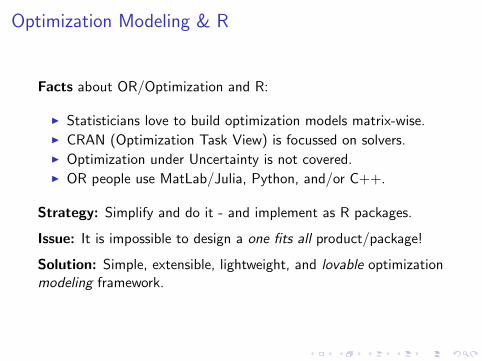
Optimization Modeling & R
Facts about OR/Optimization and R:
I Statisticians love to build optimization models matrix-wise.I CRAN (Optimization Task View) is focussed on solvers.I Optimization under Uncertainty is not covered.I OR people use MatLab/Julia, Python, and/or C++.
Strategy: Simplify and do it - and implement as R packages.
Issue: It is impossible to design a one fits all product/package!
Solution: Simple, extensible, lightweight, and lovable optimizationmodeling framework.
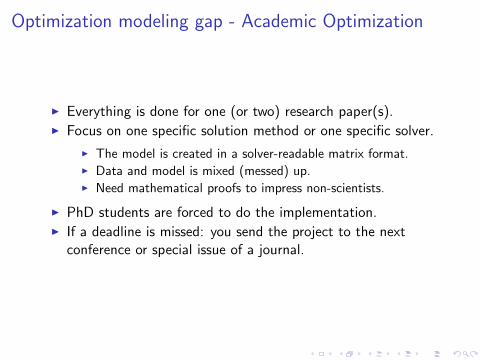
Optimization modeling gap - Academic Optimization
I Everything is done for one (or two) research paper(s).I Focus on one specific solution method or one specific solver.
I The model is created in a solver-readable matrix format.I Data and model is mixed (messed) up.I Need mathematical proofs to impress non-scientists.
I PhD students are forced to do the implementation.I If a deadline is missed: you send the project to the next
conference or special issue of a journal.
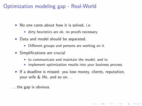
Optimization modeling gap - Real-World
I No one cares about how it is solved, i.e.
I dirty heuristics are ok, no proofs necessary.
I Data and model should be separated.
I Different groups and persons are working on it.
I Simplifications are crucial
I to communicate and maintain the model, and toI implement optimization results into your business process.
I If a deadline is missed: you lose money, clients, reputation,your wife & life, and so on. . .
. . . the gap is obvious.
Common Issue
Optimization is a side-product (“someone has to do it”).
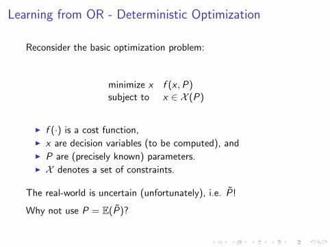
Learning from OR - Deterministic Optimization
Reconsider the basic optimization problem:
minimize x f (x ,P)subject to x ∈ X (P)
I f (·) is a cost function,I x are decision variables (to be computed), andI P are (precisely known) parameters.I X denotes a set of constraints.
The real-world is uncertain (unfortunately), i.e. P̃!
Why not use P = E(P̃)?

Learning from OR - Deterministic Optimization
Reconsider the basic optimization problem:
maximize x f (x ,P)subject to x ∈ X (P)
I f (·) is a profit function,I x are decision variables (to be computed), andI P are (precisely known) parameters.I X denotes a set of constraints.
The real-world is uncertain (unfortunately), i.e. P̃!
Why not use P = E(P̃)?
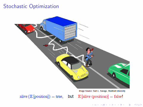
Stochastic Optimization
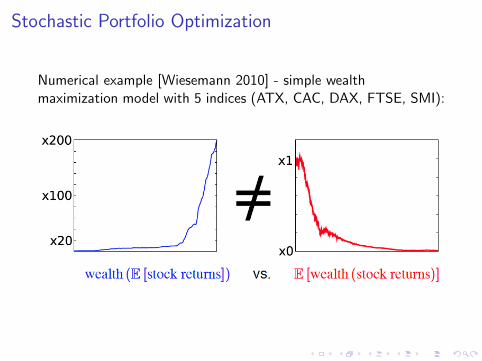
Stochastic Portfolio Optimization
Numerical example [Wiesemann 2010] - simple wealthmaximization model with 5 indices (ATX, CAC, DAX, FTSE, SMI):

Modern Portfolio Theory
Calculate an optimal portfolio x given a assets given a vector ofexpected returns M and a co-variance matrix C subject to furtherconstraints X , i.e. the well-known Markowitz approach:
minimize x x C xT
subject to x ×M ≥ µx ∈ X .
Issues with this approach:
I Uncertainty is just implicitly modeled → deterministic!I QP framework too rigid and specific (OR perspective).I General extensions (CVaR, . . . ) are put on top of this base.

Stochastic Programming - Integrating Uncertainty
Stochastic Programming naturally separates the objective andsubjective part of a decision problem.
1. Optimization model specifies the event space at eachdecision stage to integrate objective real-world constraintsand dynamics, i.e. the event handling (quantitative aspectsof the solution).
2. Uncertainty model is chosen independently fromoptimization model to reflect subjective beliefs of thedecision taker (qualitative aspects of the solution).
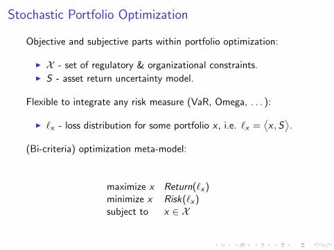
Stochastic Portfolio Optimization
Objective and subjective parts within portfolio optimization:
I X - set of regulatory & organizational constraints.I S - asset return uncertainty model.
Flexible to integrate any risk measure (VaR, Omega, . . . ):
I `x - loss distribution for some portfolio x , i.e. `x =⟨x , S
⟩.
(Bi-criteria) optimization meta-model:
maximize x Return(`x)minimize x Risk(`x)subject to x ∈ X

Optimization in R - matrix-based (modopt)
# maximize: 2*x1 + x2;
# subject to: x1+x2 <= 5;
# subject to: x1 <= 3;
# x1 >= 0, x2 >= 0
f <- c(2, 1)
A <- matrix(c(1, 1, 1, 0), nrow=2, byrow=TRUE)
b <- c(5, 3)
solution <- linprog(-f, A, b)
print(solution$x)
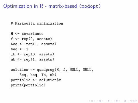
Optimization in R - matrix-based (modopt)
# Markowitz minimization
H <- covariance
f <- rep(0, assets)
Aeq <- rep(1, assets)
beq <- 1
lb <- rep(0, assets)
ub <- rep(1, assets)
solution <- quadprog(H, f, NULL, NULL,
Aeq, beq, lb, ub)
portfolio <- solution$x
print(portfolio)

Optimization Modeling in R
The ingredients of every optimization problem are:
I Parameters: Input.I Variables: Output.I Objective function(s): Minimization, Maximization.I Constraints.
Provide functions for exactly these (and only these) ingredientswithin R.
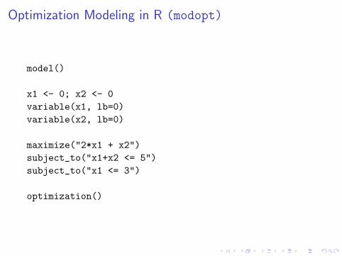
Optimization Modeling in R (modopt)
model()
x1 <- 0; x2 <- 0
variable(x1, lb=0)
variable(x2, lb=0)
maximize("2*x1 + x2")
subject_to("x1+x2 <= 5")
subject_to("x1 <= 3")
optimization()

Optimization Modeling in R with modopt
Light-weight: Just a handful of functions to add objectivefunction(s), constraints, parameters, to initialize (optimization)variables, and to define (optimization variable) sets.
I model() to create a new optimization model.I optimization() to execute the current model.
The design of the package is heavily influenced by the standaloneoptimization modeling languages AMPL and ZIMPL as well asCVX and YalMip for MatLab.
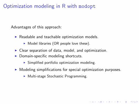
Optimization modeling in R with modopt
Advantages of this approach:
I Readable and teachable optimization models.
I Model libraries (OR people love these).
I Clear separation of data, model, and optimization.I Domain-specific modeling shortcuts.
I Simplified portfolio optimization modeling.
I Modeling simplifications for special optimization purposes.
I Multi-stage Stochastic Programming.
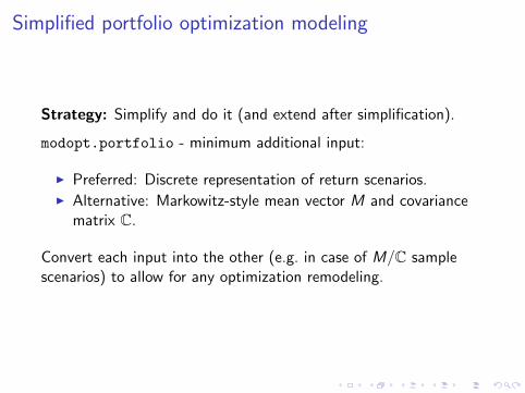
Simplified portfolio optimization modeling
Strategy: Simplify and do it (and extend after simplification).
modopt.portfolio - minimum additional input:
I Preferred: Discrete representation of return scenarios.I Alternative: Markowitz-style mean vector M and covariance
matrix C.
Convert each input into the other (e.g. in case of M/C samplescenarios) to allow for any optimization remodeling.
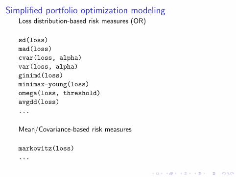
Simplified portfolio optimization modelingLoss distribution-based risk measures (OR)
sd(loss)
mad(loss)
cvar(loss, alpha)
var(loss, alpha)
ginimd(loss)
minimax-young(loss)
omega(loss, threshold)
avgdd(loss)
...
Mean/Covariance-based risk measures
markowitz(loss)
...
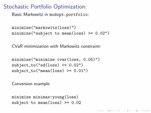
Stochastic Portfolio Optimization:Basic Markowitz in modopt.portfolio:
minimize("markowitz(loss)")
minimize("subject to mean(loss) >= 0.02")
CVaR minimization with Markowitz constraint:
minimize("minimize cvar(loss, 0.05)")
subject_to("sd(loss) <= 0.02")
subject_to("mean(loss) >= 0.01")
Conversion example:
minimize minimax-young(loss)
subject to mean(loss) >= 0.02
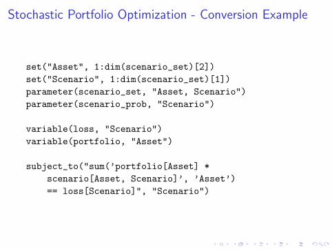
Stochastic Portfolio Optimization - Conversion Example
set("Asset", 1:dim(scenario_set)[2])
set("Scenario", 1:dim(scenario_set)[1])
parameter(scenario_set, "Asset, Scenario")
parameter(scenario_prob, "Scenario")
variable(loss, "Scenario")
variable(portfolio, "Asset")
subject_to("sum(’portfolio[Asset] *
scenario[Asset, Scenario]’, ’Asset’)
== loss[Scenario]", "Scenario")

Simplified portfolio optimization modeling
Specific additions of modopt.portfolio.minimax-young are
variable(gamma)
variable(scenario_downside, "Scenario", lb=0)
subject_to("scenario_downside[Scenario] - gamma +
loss[Scenario] >= 0", "Scenario")
maximize("gamma")
optimization() will calculate the optimal portfolio but alsoprovide the optimization model within R for further modification.
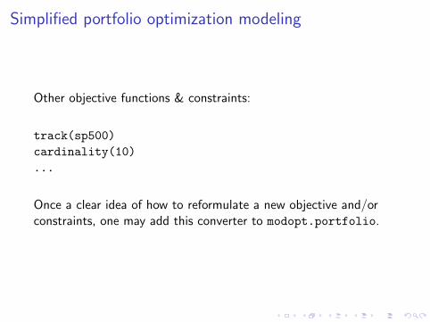
Simplified portfolio optimization modeling
Other objective functions & constraints:
track(sp500)
cardinality(10)
...
Once a clear idea of how to reformulate a new objective and/orconstraints, one may add this converter to modopt.portfolio.
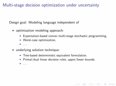
Multi-stage decision optimization under uncertainty
Design goal: Modeling language independent of
I optimization modeling approach:
I Expectation-based convex multi-stage stochastic programming,I Worst-case optimization,I . . .
I underlying solution technique:
I Tree-based deterministic equivalent formulation.I Primal/dual linear decision rules, upper/lower bounds.I . . .
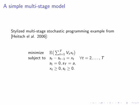
A simple multi-stage model
Stylized multi-stage stochastic programming example from[Heitsch el al. 2006]:
minimize E(∑T
t=1 Vtxt)
subject to st − st−1 = xt ∀t = 2, . . . ,Ts1 = 0, sT = a,xt ≥ 0, st ≥ 0.

A simple multi-stage model in R (modopt.multistage)
parameter(a)
variable(x, lb=0); variable(s, lb=0)
maximize(id="objective", "E(x)")
subject_to(id="non_anticitpativity", "s - s(-1) = x")
subject_to(id="root_stage", "s = 0")
subject_to(id="terminal_stage", "s = a")
deterministic("T", a)
stochastic("0..T", x, s, "objective")
stochastic("1..T", "non_anticipativity")
stochastic("0", "root_stage")
stochastic("T", "terminal_stage")
Contact
Ronald Hochreiter
WU Vienna University of Economics and Business
Augasse 2-6, 1090 Vienna, Austria
http://www.finance-r.com/
http://www.modopt.com/