Ronny Kohavi, ICML 1998

Ronny Kohavi, ICML 1998

Ronny Kohavi, ICML 1998

What is Data mining?

ResearchQuestion

Find Data

Internal Databases

Data Warehouses

InternetOnline databases

Data Collection

Data ProcessingExtract Information

Data Analysis

AnswerResearch Question

Outline

• Data MiningData Mining

• Methodology for CARTMethodology for CART

• Data mining trees, tree sketchesData mining trees, tree sketches

•Applications to clinical data. Applications to clinical data.

•Categorical Response - OAB data Categorical Response - OAB data

•Continuous Response - Geodon RCT data Continuous Response - Geodon RCT data

• Robustness issues Robustness issues

•Processing “capacity” doubles every couple of years (Exponential)•Hard Disk storage “capacity” doubles every 18 months (Use to be every 36 months)

•Bottle necks are not speed anymore. •Processing capacity is not growing as fast as data acquisition.

Moore’s law:

+

-

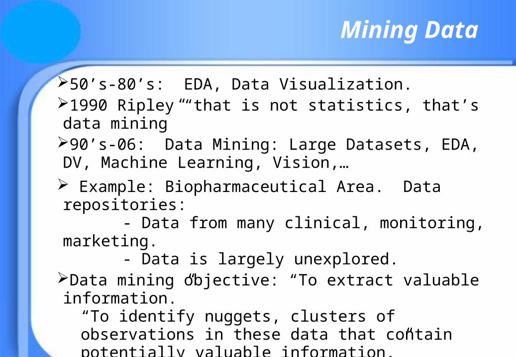
50’s-80’s: EDA, Data Visualization.1990 Ripley “that is not statistics, that’s data mining”90’s-06: Data Mining: Large Datasets, EDA, DV, Machine Learning, Vision,…

Example: Biopharmaceutical Area. Data repositories: - Data from many clinical, monitoring, marketing.- Data is largely unexplored.

Data mining objective: “To extract valuable information.”“To identify nuggets, clusters of observations in these data that contain potentially valuable information.”

Example: Biopharmaceutical Data:- Extract new information from existing databases.- Answer questions of clinicians, marketing.- Help design new studies.

Mining Data

Data Mining Software and Recursive Partition

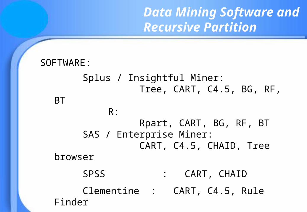
SOFTWARE:

Splus / Insightful Miner: Tree, CART, C4.5, BG, RF, BT

R: Rpart, CART, BG, RF, BT

SAS / Enterprise Miner:CART, C4.5, CHAID, Tree

browser

SPSS : CART, CHAID

Clementine : CART, C4.5, Rule Finder

HelixTree : CART, FIRM, BG, RF, BT

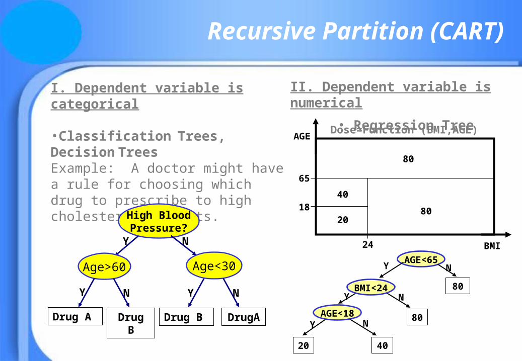
I. Dependent variable is categorical •Classification Trees, Decision Trees Example: A doctor might have a rule for choosing which drug to prescribe to high cholesterol patients.

Recursive Partition (CART)

II. Dependent variable is numerical 

• Regression Tree

20

80

80

40

65

18

BMI

AGEDose=Function (BMI,AGE)

High BloodPressure?

Age>60

DrugA

Age<30

Drug A

Y

Y

Y NN

N

Drug B Drug B

24

AGE<65

80

80

BMI<24

AGE<18

4020

Y

Y

Y

N

N

N

?Y N

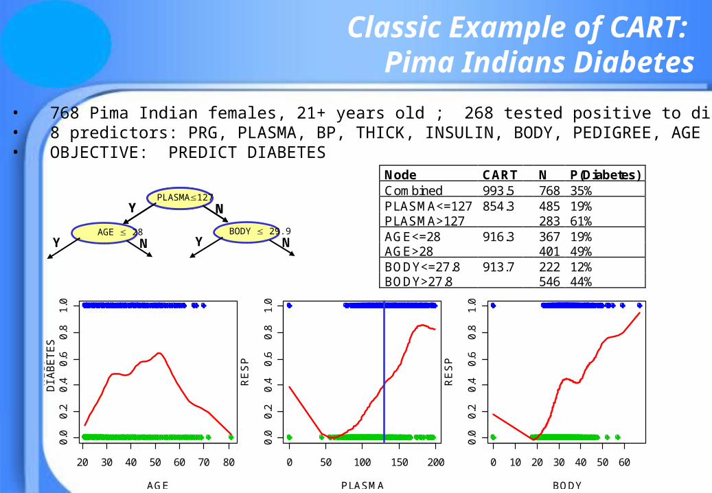
Classic Example of CART: Pima Indians Diabetes

• 768 Pima Indian females, 21+ years old ; 268 tested positive to diabetes• 8 predictors: PRG, PLASMA, BP, THICK, INSULIN, BODY, PEDIGREE, AGE• OBJECTIVE: PREDICT DIABETES

Node CART N P(Diabetes) Combined 993.5 768 35% PLASMA<=127 854.3 485 19% PLASMA>127 283 61% AGE<=28 916.3 367 19% AGE>28 401 49% BODY<=27.8 913.7 222 12% BODY>27.8 546 44%

PLASMA127Y N

AGE 28Y N

BODY 29.9Y N

20 30 40 50 60 70 80

0.0

0.2

0.4

0.6

0.8

1.0

AGE

RE

SP

0 50 100 150 200

0.0

0.2

0.4

0.6

0.8

1.0

PLASMA

RE

SP

0 10 20 30 40 50 600.

00.

20.

40.

60.

81.

0BODY

RE

SP

DIA

BE

TE

S

Classic Example of CART: Pima Indians Diabetes

|PLASMA<127.5

AGE<28.5

BODY<30.95 BODY<26.35

PLASMA<99.5

PEDIGREE<0.561

BODY<29.95

PLASMA<145.5 PLASMA<157.5

AGE<30.5

BP<61

0.01325 0.17500 0.04878

0.18180

0.40480 0.73530

0.14630 0.51430

1.00000 0.32500

0.72310

0.86960

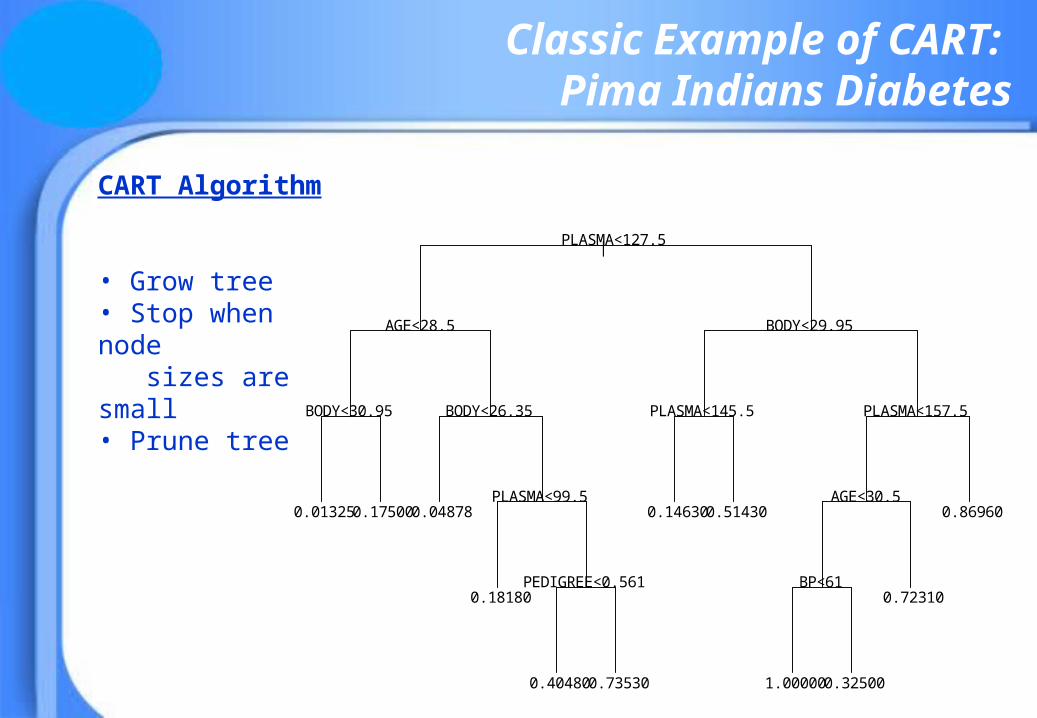
CART Algorithm

 • Grow tree• Stop when node sizes are small• Prune tree

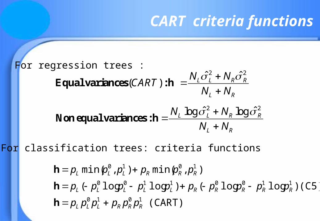
CART criteria functions

2 2ˆ ˆ( ) L L R R

L R

N NCART

N N

Equal variances : h

For classification trees: criteria functions

2 2ˆ ˆlog logL L R R

L R

N N

N N

Non equal variances : h

(CART)

(C5) )loglog()loglog(

),min(),min(

1010

11001100

1010

RRRLLL

RRRRRLLLLL

RRRLLL

pppppp

pppppppppp

pppppp

h

h

h

For regression trees :

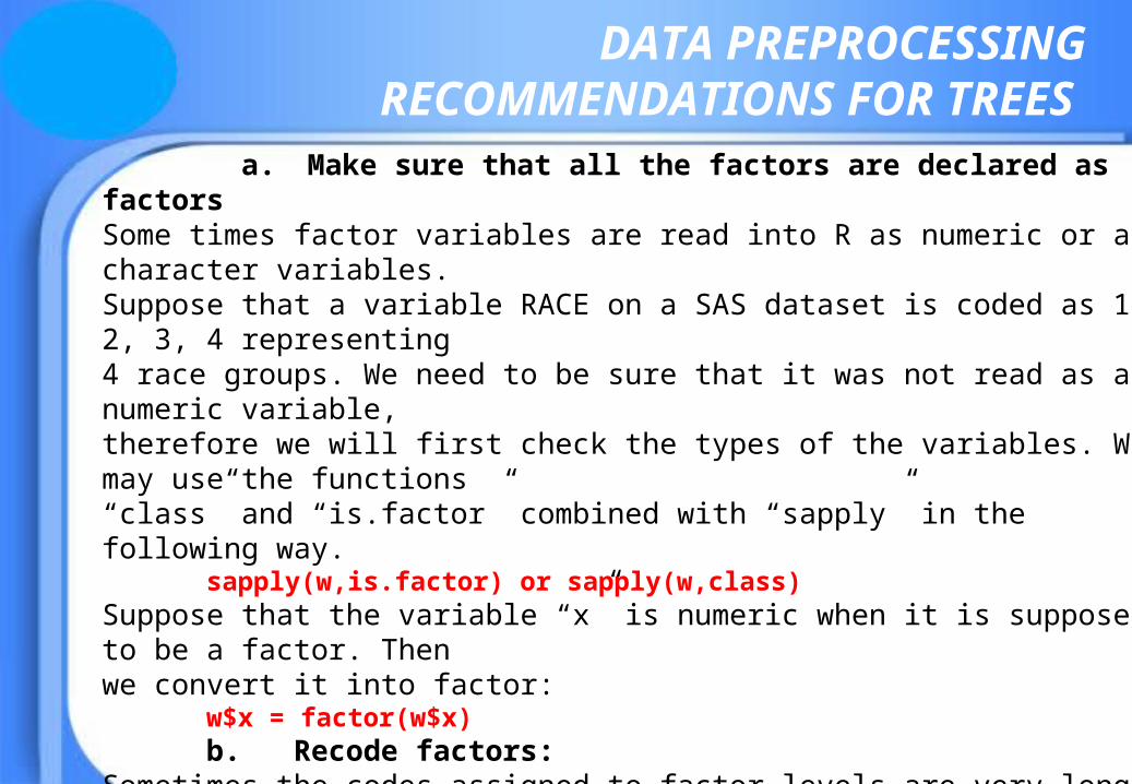
a.   Make sure that all the factors are declared as factorsSome times factor variables are read into R as numeric or as character variables. Suppose that a variable RACE on a SAS dataset is coded as 1, 2, 3, 4 representing4 race groups. We need to be sure that it was not read as a numeric variable,therefore we will first check the types of the variables. We may use the functions“class” and “is.factor” combined with “sapply” in the following way. sapply(w,is.factor) or sapply(w,class)Suppose that the variable “x” is numeric when it is supposed to be a factor. Thenwe convert it into factor:

w$x = factor(w$x) b.   Recode factors: Sometimes the codes assigned to factor levels are very long phrases and when those codes are inserted into the tree the resulting graph can be very messy. We prefer to use short words to represent the codes. To recode the factor levels you may use the function “f.recode”: > levels(w$Muscle)

[1] "" "Mild Weakness" [3] "Moderate Weakness" "Normal"

> musc =f.recode(w$Muscle,c("","Mild","Mod","Norm")) > w$Musclenew = musc

DATA PREPROCESSING RECOMMENDATIONS FOR TREES

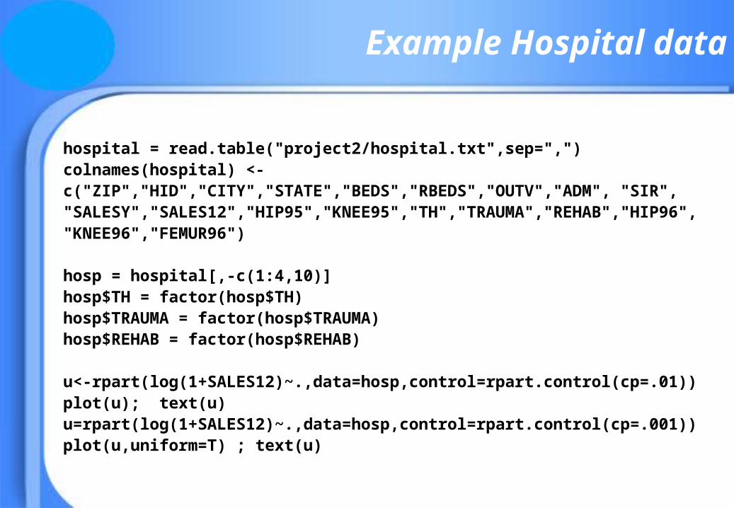
hospital = read.table("project2/hospital.txt",sep=",")colnames(hospital) <-c("ZIP","HID","CITY","STATE","BEDS","RBEDS","OUTV","ADM", "SIR","SALESY","SALES12","HIP95","KNEE95","TH","TRAUMA","REHAB","HIP96","KNEE96","FEMUR96")

hosp = hospital[,-c(1:4,10)]hosp$TH = factor(hosp$TH) hosp$TRAUMA = factor(hosp$TRAUMA) hosp$REHAB = factor(hosp$REHAB)  u<-rpart(log(1+SALES12)~.,data=hosp,control=rpart.control(cp=.01))plot(u); text(u)u=rpart(log(1+SALES12)~.,data=hosp,control=rpart.control(cp=.001))plot(u,uniform=T) ; text(u)

Example Hospital data

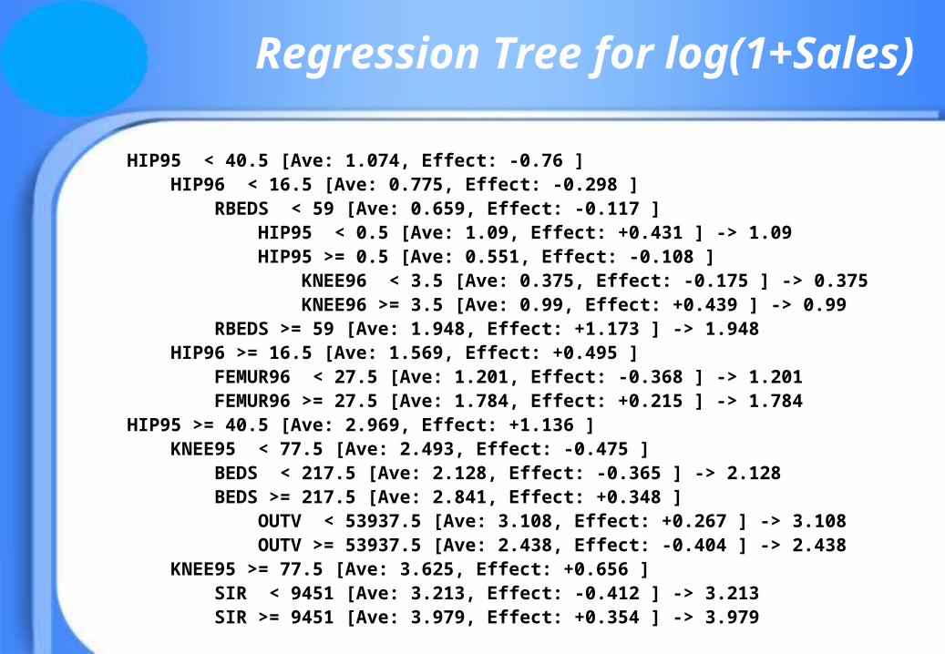
HIP95 < 40.5 [Ave: 1.074, Effect: -0.76 ] HIP96 < 16.5 [Ave: 0.775, Effect: -0.298 ] RBEDS < 59 [Ave: 0.659, Effect: -0.117 ] HIP95 < 0.5 [Ave: 1.09, Effect: +0.431 ] -> 1.09 HIP95 >= 0.5 [Ave: 0.551, Effect: -0.108 ] KNEE96 < 3.5 [Ave: 0.375, Effect: -0.175 ] -> 0.375 KNEE96 >= 3.5 [Ave: 0.99, Effect: +0.439 ] -> 0.99 RBEDS >= 59 [Ave: 1.948, Effect: +1.173 ] -> 1.948 HIP96 >= 16.5 [Ave: 1.569, Effect: +0.495 ] FEMUR96 < 27.5 [Ave: 1.201, Effect: -0.368 ] -> 1.201 FEMUR96 >= 27.5 [Ave: 1.784, Effect: +0.215 ] -> 1.784HIP95 >= 40.5 [Ave: 2.969, Effect: +1.136 ] KNEE95 < 77.5 [Ave: 2.493, Effect: -0.475 ] BEDS < 217.5 [Ave: 2.128, Effect: -0.365 ] -> 2.128 BEDS >= 217.5 [Ave: 2.841, Effect: +0.348 ] OUTV < 53937.5 [Ave: 3.108, Effect: +0.267 ] -> 3.108 OUTV >= 53937.5 [Ave: 2.438, Effect: -0.404 ] -> 2.438 KNEE95 >= 77.5 [Ave: 3.625, Effect: +0.656 ] SIR < 9451 [Ave: 3.213, Effect: -0.412 ] -> 3.213 SIR >= 9451 [Ave: 3.979, Effect: +0.354 ] -> 3.979

Regression Tree for log(1+Sales)

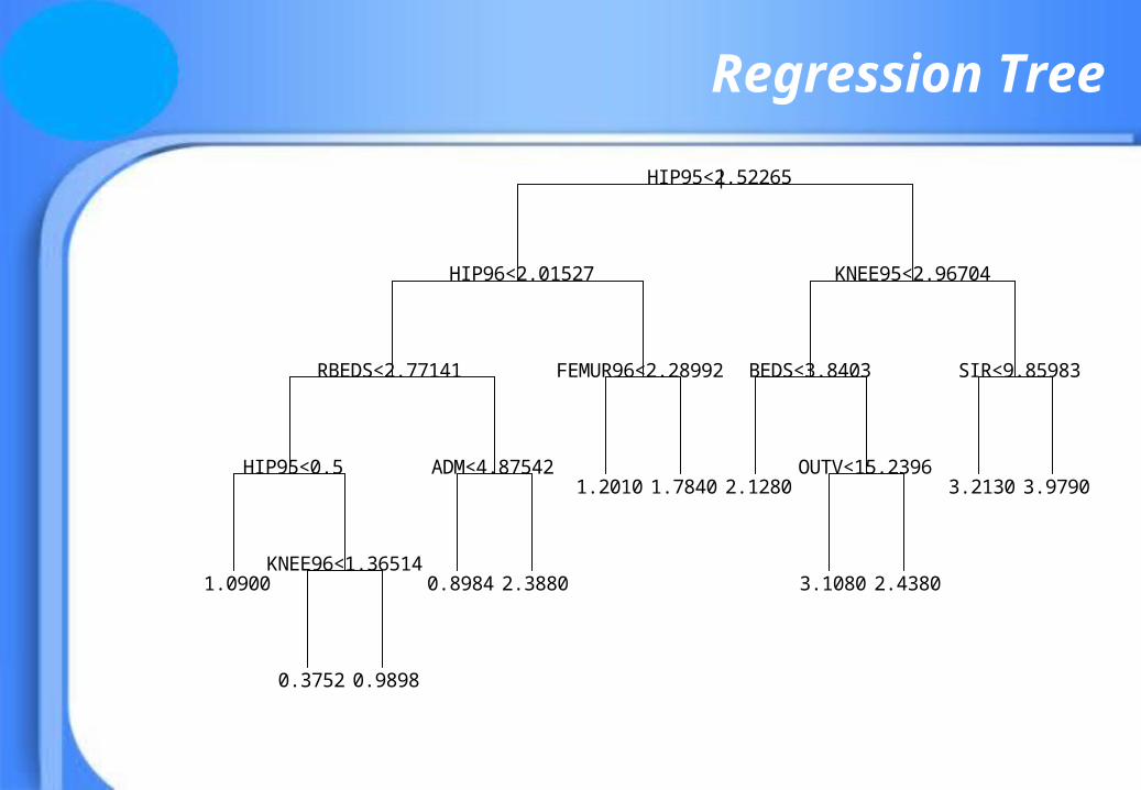
|HIP95<2.52265

HIP96<2.01527

RBEDS<2.77141

HIP95<0.5

KNEE96<1.36514

ADM<4.87542

FEMUR96<2.28992

KNEE95<2.96704

BEDS<3.8403

OUTV<15.2396

SIR<9.85983

1.0900

0.3752 0.9898

0.8984 2.3880

1.2010 1.7840 2.1280

3.1080 2.4380

3.2130 3.9790

Regression Tree

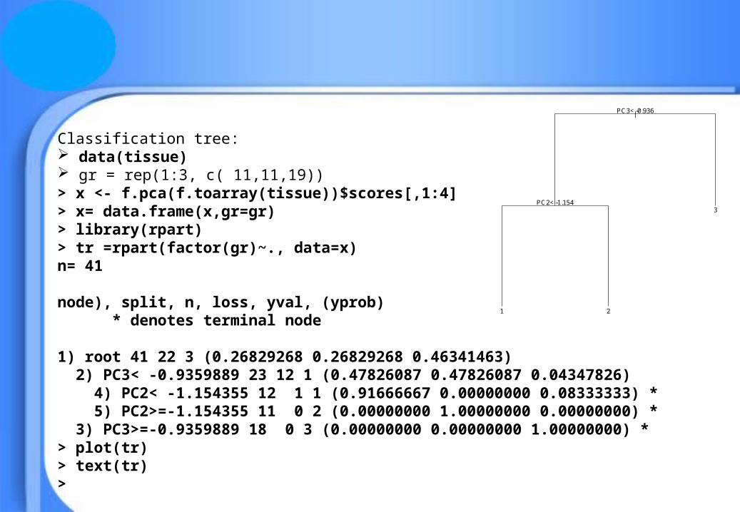
Classification tree: data(tissue) gr = rep(1:3, c( 11,11,19))> x <- f.pca(f.toarray(tissue))$scores[,1:4]> x= data.frame(x,gr=gr)> library(rpart)> tr =rpart(factor(gr)~., data=x)n= 41  node), split, n, loss, yval, (yprob) * denotes terminal node 1) root 41 22 3 (0.26829268 0.26829268 0.46341463) 2) PC3< -0.9359889 23 12 1 (0.47826087 0.47826087 0.04347826) 4) PC2< -1.154355 12 1 1 (0.91666667 0.00000000 0.08333333) * 5) PC2>=-1.154355 11 0 2 (0.00000000 1.00000000 0.00000000) * 3) PC3>=-0.9359889 18 0 3 (0.00000000 0.00000000 1.00000000) *> plot(tr)> text(tr)>

|PC3< -0.936

PC2< -1.154

1 2

3

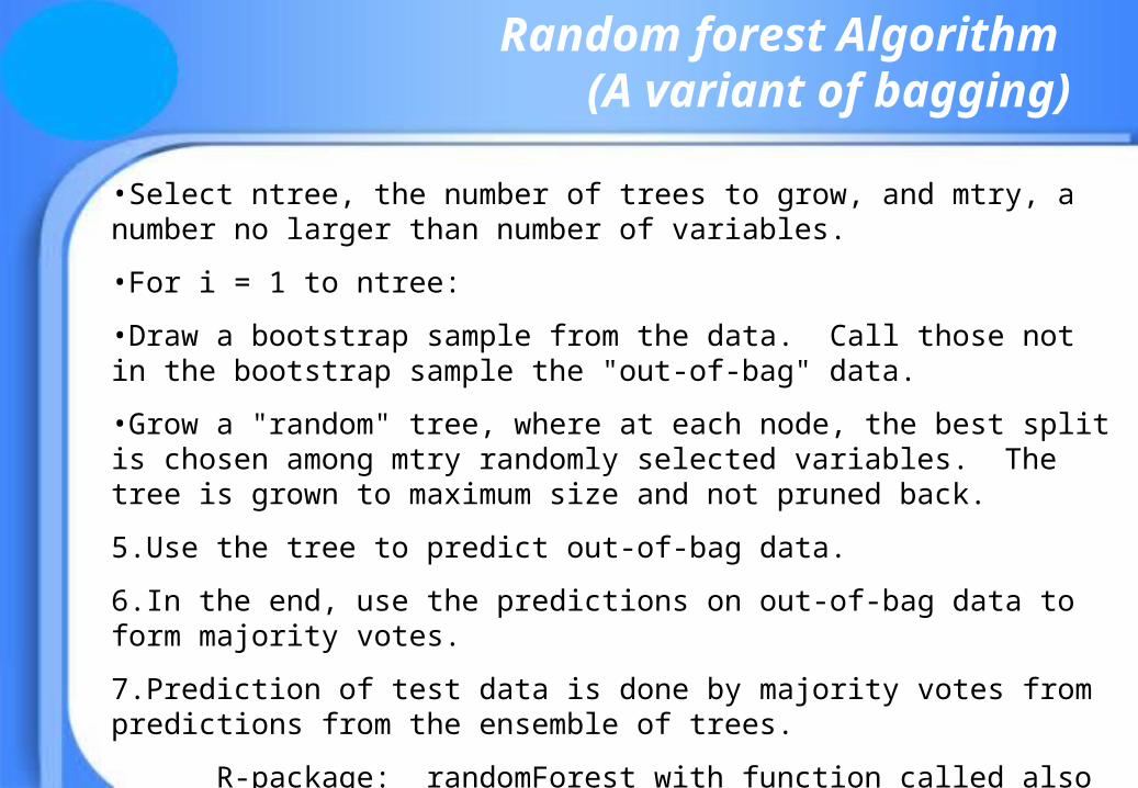
Random forest Algorithm (A variant of bagging)

•Select ntree, the number of trees to grow, and mtry, a number no larger than number of variables.

•For i = 1 to ntree:

•Draw a bootstrap sample from the data. Call those not in the bootstrap sample the "out-of-bag" data.

•Grow a "random" tree, where at each node, the best split is chosen among mtry randomly selected variables. The tree is grown to maximum size and not pruned back.

5.Use the tree to predict out-of-bag data.

6.In the end, use the predictions on out-of-bag data to form majority votes.

7.Prediction of test data is done by majority votes from predictions from the ensemble of trees.

R-package: randomForest with function called also randomForest

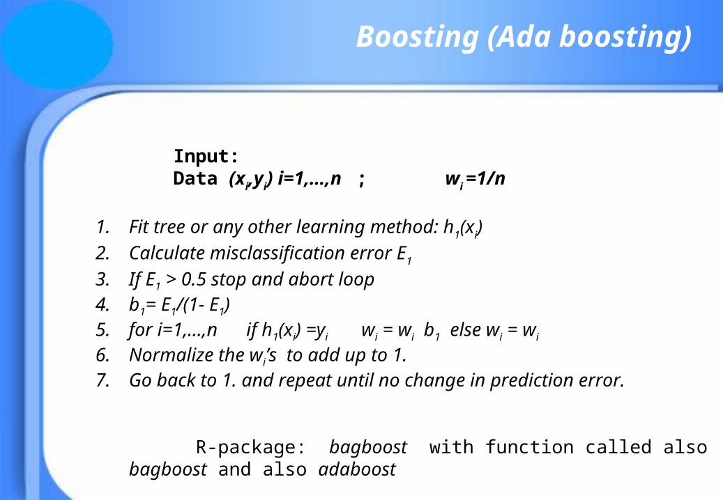
Input: Data (xi,yi) i=1,…,n ; wi =1/n

1. Fit tree or any other learning method: h1(xi)2. Calculate misclassification error E1

3. If E1 > 0.5 stop and abort loop4. b1= E1/(1- E1)5. for i=1,…,n if h1(xi) =yi wi = wi b1 else wi = wi 6. Normalize the wi’s to add up to 1.7. Go back to 1. and repeat until no change in prediction error.

R-package: bagboost with function called also bagboost and also adaboost

Boosting (Ada boosting)

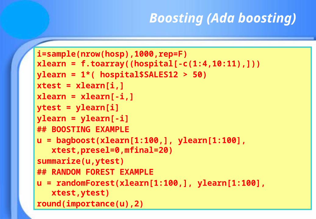
i=sample(nrow(hosp),1000,rep=F)xlearn = f.toarray((hospital[-c(1:4,10:11),]))ylearn = 1*( hospital$SALES12 > 50)xtest = xlearn[i,]xlearn = xlearn[-i,]ytest = ylearn[i]ylearn = ylearn[-i]## BOOSTING EXAMPLEu = bagboost(xlearn[1:100,], ylearn[1:100],

xtest,presel=0,mfinal=20)summarize(u,ytest)## RANDOM FOREST EXAMPLEu = randomForest(xlearn[1:100,], ylearn[1:100],

xtest,ytest) round(importance(u),2)

Boosting (Ada boosting)

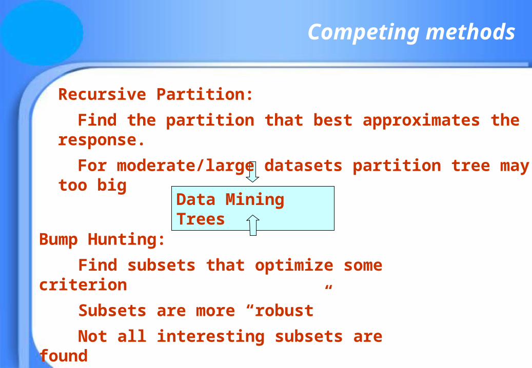
Competing methods

Bump Hunting:

Find subsets that optimize some criterion

Subsets are more “robust”

Not all interesting subsets are found

Data Mining Trees

Recursive Partition:

Find the partition that best approximates the response.

For moderate/large datasets partition tree may be too big

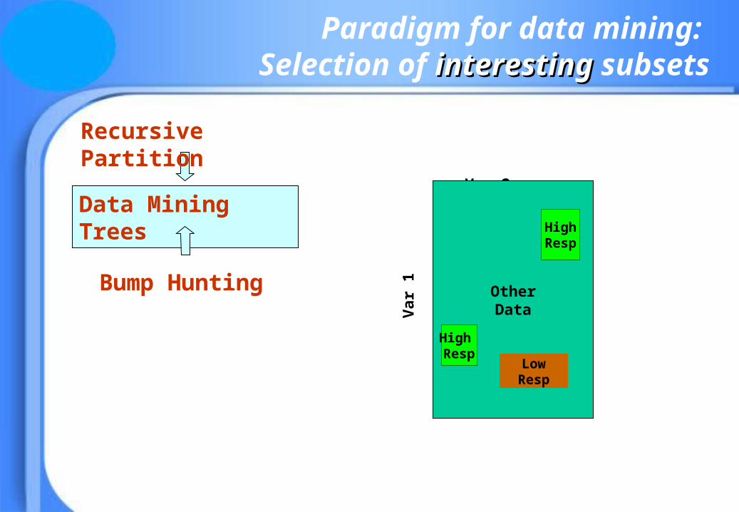
Paradigm for data mining: Selection of interestinginteresting subsets

Bump Hunting

Data Mining Trees

Recursive Partition

Var 2

OtherData

High Resp

Var

1

HighResp

LowResp

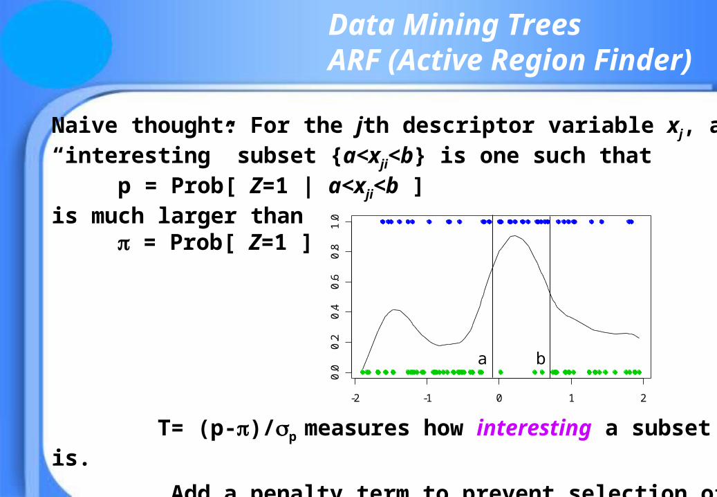
Naive thought: For the jth descriptor variable xj, an “interesting” subset {a<xji<b} is one such that p = Prob[ Z=1 | a<xji<b ]is much larger than = Prob[ Z=1 ]

T= (p-)/p measures how interesting a subset is. 

Add a penalty term to prevent selection of subsets that are too small or too large.

Data Mining TreesARF (Active Region Finder)

-2 -1 0 1 2

0.0

0.2

0.4

0.6

0.8

1.0

x

y

a b

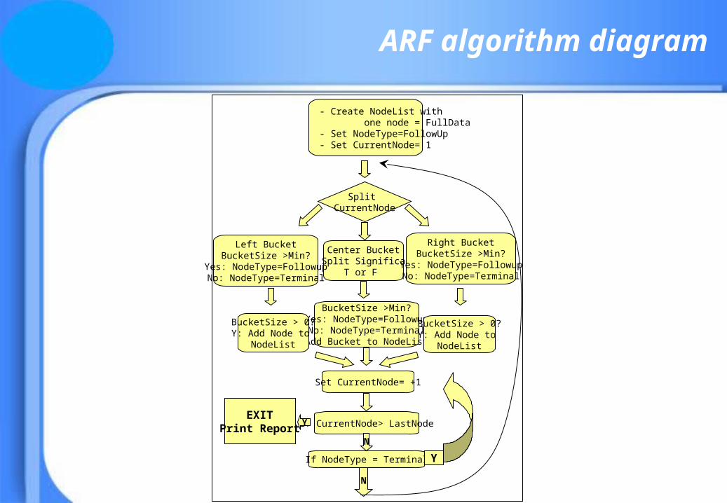
- Create NodeList with one node = FullData- Set NodeType=FollowUp- Set CurrentNode= 1

Split CurrentNode

Center BucketIs Split Significant?

T or F

BucketSize >Min?Yes: NodeType=FollowupNo: NodeType=TerminalAdd Bucket to NodeList

Left BucketBucketSize >Min?

Yes: NodeType=FollowupNo: NodeType=Terminal

BucketSize > 0?Y: Add Node to

NodeList

Right BucketBucketSize >Min?

Yes: NodeType=FollowupNo: NodeType=Terminal

BucketSize > 0?Y: Add Node to

NodeList

Set CurrentNode= +1

If NodeType = Terminal Y

N

if CurrentNode> LastNodeYEXIT

Print ReportN

ARF algorithm diagram

20 30 40 50 60 70 80

-50

050

x

20 30 40 50 60 70 80

020

4060

x

20 30 40 50 60 70 80

-50

050

20 30 40 50 60 70 80

0.0

0.4

0.8

x

y1

20 30 40 50 60 70 80

0.0

0.4

0.8

x

y3

20 30 40 50 60 70 80

0.0

0.4

0.8

y5

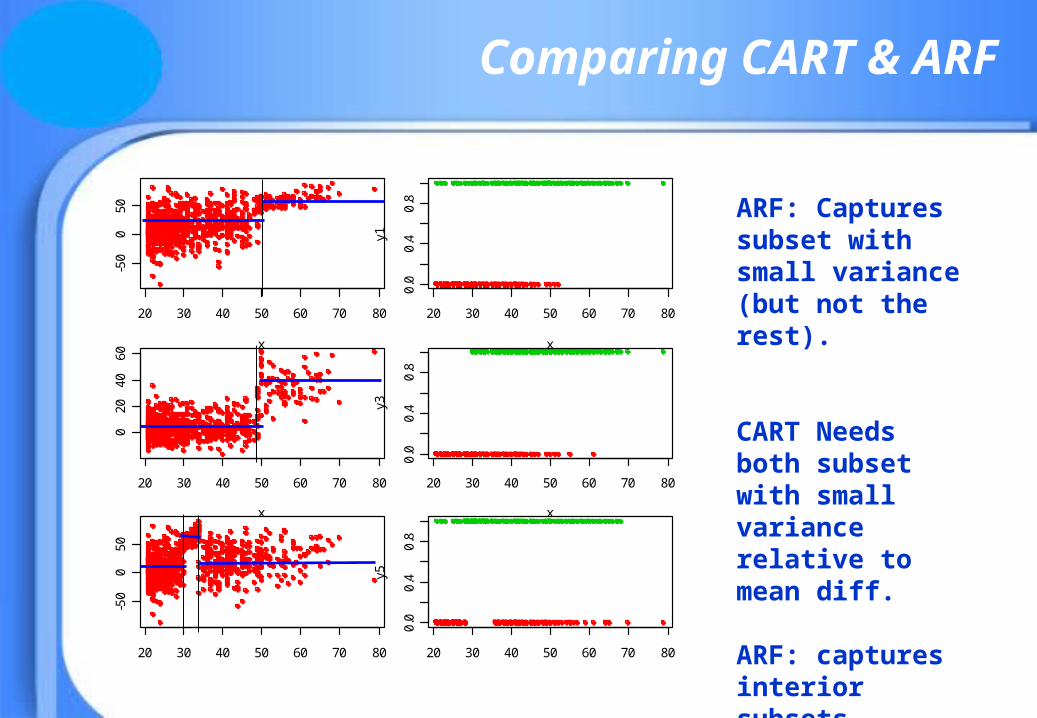
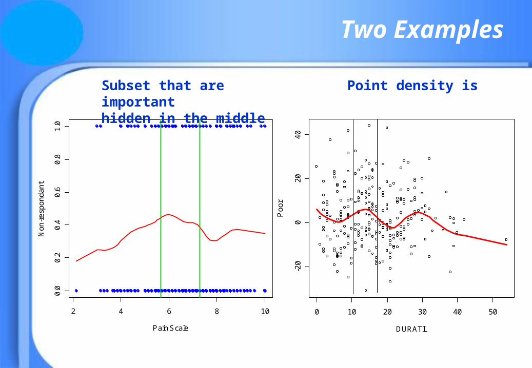
Comparing CART & ARF

ARF: Captures subset with small variance (but not the rest).

CART Needs both subset with small variance relative to mean diff. ARF: captures interior subsets.

2 4 6 8 10

0.0

0.2

0.4

0.6

0.8

1.0

Pain Scale

No

n-r

esp

on

da

nt

Two Examples

0 10 20 30 40 50

-20

02

04

0

DURATIL

Po

or

Subset that are Point density is important hidden in the middle

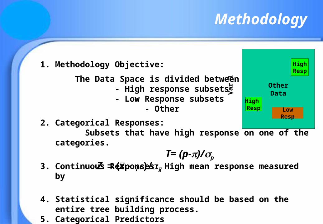
1. Methodology Objective:

The Data Space is divided between - High response subsets- Low Response subsets

- Other

2. Categorical Responses:Subsets that have high response on one of the

categories.

T= (p-)/p

3. Continuous Responses: High mean response measured by

4. Statistical significance should be based on the entire tree building process.

5. Categorical Predictors6. Data Visualization7. PDF report.

Methodology

Var 2

OtherData

High Resp

Var

1

HighResp

LowResp

( ) / xZ x

Report

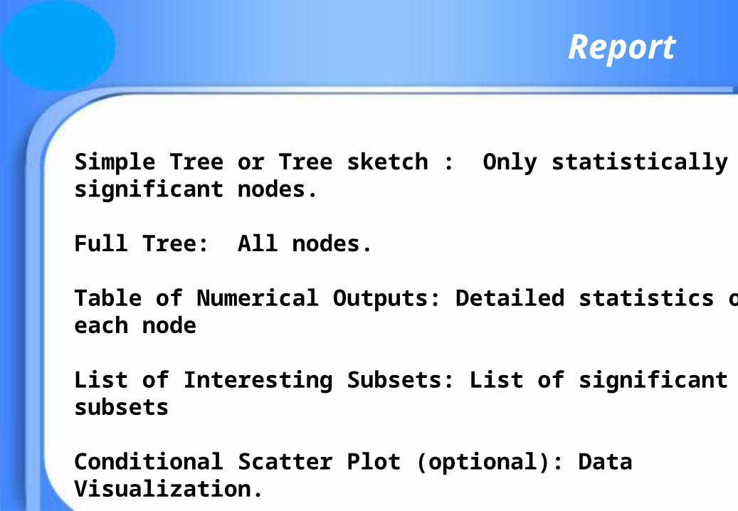
Simple Tree or Tree sketch : Only statistically significant nodes.

Full Tree: All nodes.

Table of Numerical Outputs: Detailed statistics of each node

List of Interesting Subsets: List of significant subsets

Conditional Scatter Plot (optional): Data Visualization.

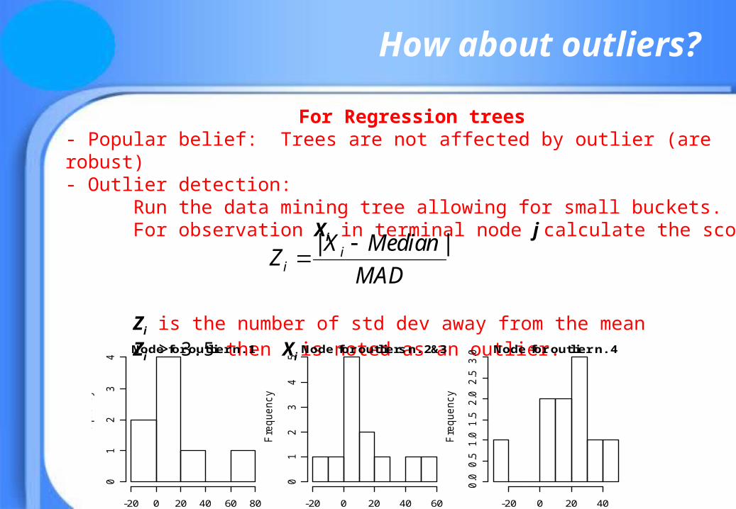
How about outliers?

For Regression trees- Popular belief: Trees are not affected by outlier (are robust)- Outlier detection: Run the data mining tree allowing for small buckets. For observation Xi in terminal node j calculate the score

Zi is the number of std dev away from the meanZi > 3.5 then Xi is noted as an outlier.

| | i

i

X MedianZ

MAD

Node for outlier n. 1

Fre

quency

-20 0 20 40 60 80

01

23

4

Node for outliers n. 2&3

Fre

quency

-20 0 20 40 60

01

23

45

Node for outlier n. 4

Fre

quency

-20 0 20 40

0.0

0.5

1.0

1.5

2.0

2.5

3.0

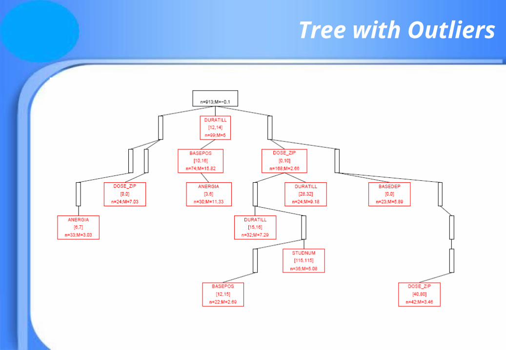
Tree with Outliers

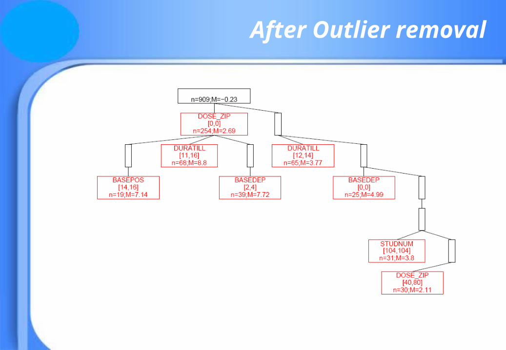
After Outlier removal

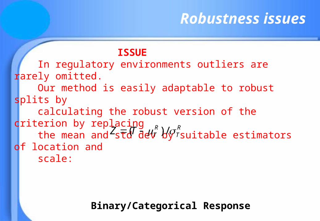
Robustness issues

ISSUE In regulatory environments outliers are rarely omitted. Our method is easily adaptable to robust splits by calculating the robust version of the criterion by replacing the mean and std dev by suitable estimators of location and scale:

Binary/Categorical Response

- How do we think about Robustness of trees? - One outlier might not make any difference. - 5% , 10% or more outliers could make a difference.

( ) /R RT TZ T

Further work

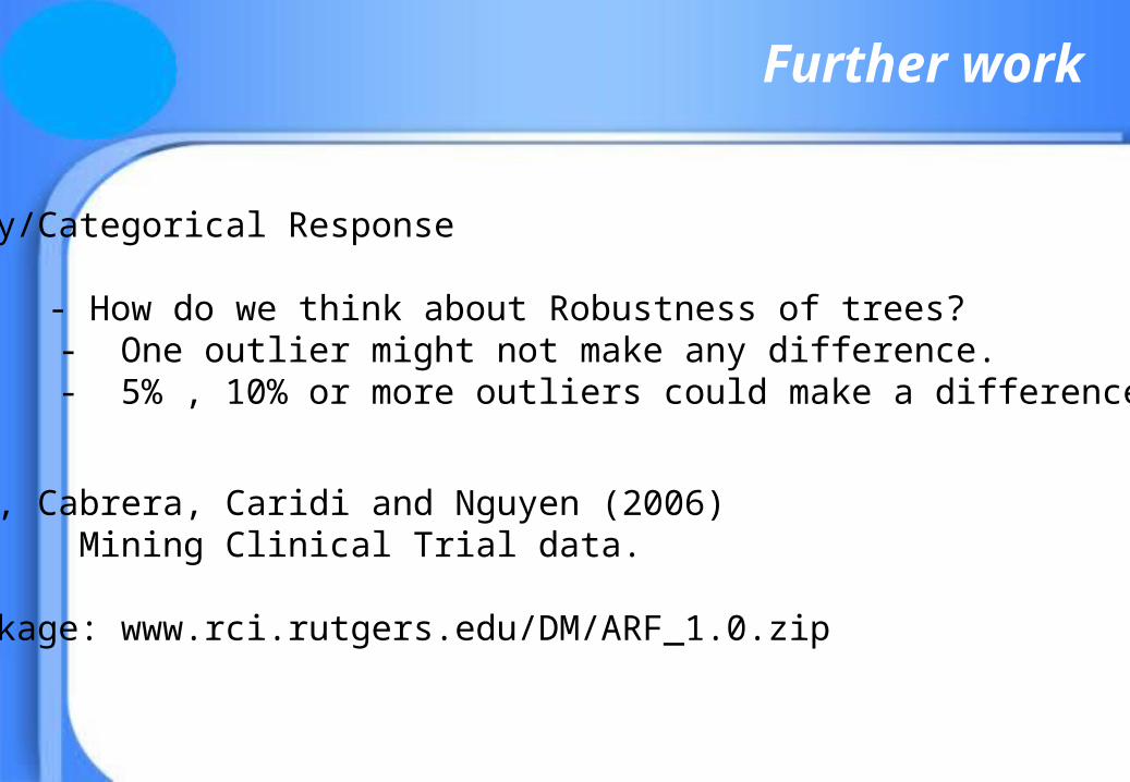
Binary/Categorical Response

- How do we think about Robustness of trees? - One outlier might not make any difference. - 5% , 10% or more outliers could make a difference.

Alvir, Cabrera, Caridi and Nguyen (2006) Mining Clinical Trial data.

R-package: www.rci.rutgers.edu/DM/ARF_1.0.zip