Embed Size (px)
Citation preview
Astronomy & Astrophysics manuscript no. AA201322646 c©ESO 2018November 8, 2018
Rotationally-supported disks around Class I sources in Taurus:disk formation constraints ?
D. Harsono1, 2, J. K. Jørgensen3, 4, E. F. van Dishoeck1, 5, M. R. Hogerheijde1, S. Bruderer5, M. V. Persson1, 3, 4, andJ. C. Mottram1
1 Leiden Observatory, Leiden University, P.O. Box 9513, 2300 RA Leiden, The Netherlands e-mail: : [email protected] SRON Netherlands Institute for Space Research, PO Box 800, 9700 AV, Groningen, The Netherlands3 Niels Bohr Institute, University of Copenhagen, Juliane Maries Vej 30, 2100 Copenhagen Ø, Denmark4 Centre for Star and Planet Formation, Natural History Museum of Denmark, University of Copenhagen, Øster Voldgade 5-7, 1350
Copenhagen K, Denmark5 Max-Planck-Institut für extraterretrische Physik, Giessenbachstrasse 1, 85748, Garching, Germany
November 8, 2018
ABSTRACT
Context. Disks are observed around pre-main sequence stars, but how and when they form is still heavily debated. While disks aroundyoung stellar objects have been identified through thermal dust emission, spatially and spectrally resolved molecular line observationsare needed to determine their nature. Only a handful of embedded rotationally supported disks have been identified to date.Aims. We identify and characterize rotationally supported disks near the end of the main accretion phase of low-mass protostars bycomparing their gas and dust structures.Methods. Subarcsecond observations of dust and gas toward four Class I low-mass young stellar objects in Taurus are presented atsignificantly higher sensitivity than previous studies. The 13CO and C18O J = 2–1 transitions at 220 GHz were observed with thePlateau de Bure Interferometer at a spatial resolution of ≤0.8′′ (56 AU radius at 140 pc) and analyzed using uv-space position velocitydiagrams to determine the nature of their observed velocity gradient.Results. Rotationally supported disks (RSDs) are detected around 3 of the 4 Class I sources studied. The derived masses identify themas Stage I objects; i.e., their stellar mass is higher than their envelope and disk masses. The outer radii of the Keplerian disks towardour sample of Class I sources are ≤ 100 AU. The lack of on-source C18O emission for TMR1 puts an upper limit of 50 AU on itssize. Flattened structures at radii > 100 AU around these sources are dominated by infalling motion (υ ∝ r−1). A large-scale envelopemodel is required to estimate the basic parameters of the flattened structure from spatially resolved continuum data. Similarities anddifferences between the gas and dust disk are discussed. Combined with literature data, the sizes of the RSDs around Class I objectsare best described with evolutionary models with an initial rotation of Ω = 10−14 Hz and slow sound speeds. Based on the comparisonof gas and dust disk masses, little CO is frozen out within 100 AU in these disks.Conclusions. Rotationally supported disks with radii up to 100 AU are present around Class I embedded objects. Larger surveys ofboth Class 0 and I objects are needed to determine whether most disks form late or early in the embedded phase.
Key words. stars: low-mass – stars: protostars – accretion, accretion disks – techniques: interferometric – ISM: molecules – proto-planetary disks
1. Introduction
Rotationally supported accretion disks (RSDs) are thought toform very early during the star formation process (see, e.g., Bo-denheimer 1995). The RSD transports a significant fraction ofthe mass from the envelope onto the young star and eventuallyevolves into a protoplanetary disk as the envelope dissipates. Thepresence of an RSD affects not only the physical structure of thesystem but also the chemical content and evolution as it pro-motes the production of more complex chemical species by pro-viding a longer lifespan at mildly elevated temperature (Aikawaet al. 2008; Visser et al. 2011; Aikawa et al. 2011). Although thestandard picture of star formation predicts early formation andevolution of RSDs, theoretical studies suggest that the presenceof magnetic fields prevents the formation of RSDs in the earlystages of star formation (e.g., Galli & Shu 1993; Chiang et al.? Based on observations carried out with the IRAM Plateau de Bure
Interferometer. IRAM is supported by INSU/CNBRS(France), MPG(Germany) and IGN (Spain).
2008; Li et al. 2011; Joos et al. 2012). Unstable flattened disk-like structures are formed in such simulations, and indeed, disksin the embedded phase have been inferred through continuumobservations (e.g., Looney et al. 2003; Jørgensen et al. 2009;Enoch et al. 2011; Chiang et al. 2012). However, with only con-tinuum data, it is difficult to distinguish between such a featureand an RSD. Thus, spatially and spectrally resolved observationsof the gas are needed to unravel the nature of these embeddeddisks.
Only a handful of studies have explored the change in thevelocity profiles from the envelope to the disk with spectrally re-solved molecular lines (Lee 2010; Yen et al. 2013; Murillo et al.2013). It is essential to differentiate between the disk and theinfalling envelope through such analysis. This paper presentsIRAM Plateau de Bure Interferometer (PdBI) observations of13CO and C18O J =2–1 toward four Class I sources in Taurus(d = 140 pc) at higher angular resolution (∼0.8′′ = 112 AUdiameter at 140 pc) and higher sensitivity than previously pos-sible. We aim to study the velocity profile as revealed through
Article number, page 1 of 22
arX
iv:1
312.
5716
v1 [
astr
o-ph
.GA
] 1
9 D
ec 2
013
A&A proofs: manuscript no. AA201322646
these molecular lines and constrain the size of embedded RSDstoward these sources.
The embedded phase can be divided into the following stages(Robitaille et al. 2006): Stage 0 (Menv > M?), Stage I (Menv <M? but Mdisk < Menv) and Stage II (Menv < Mdisk), whereM?, Menv and Mdisk are masses of the central protostar, envelopand RSD respectively. This is not to be confused with Classes,which are observationally derived evolutionary indicators (Lada& Wilking 1984; Andre et al. 1993) that do not necessarily traceevolutionary stage due to geometrical effects (Whitney et al.2003; Crapsi et al. 2008; Dunham et al. 2010). However, sinceall Class I sources discussed in this paper also turn out to be trueStage I sources, we use the Class notation throughout this paperfor convenience.
RSDs are ubiquitous once most of the envelope has beendissipated away (Class II) with outer radius Rout up to approxi-mately 200 AU (Williams & Cieza 2011, and references therein).On the other hand, the general kinematical structure of deeplyembedded protostars on small scales is still not well understood.There is growing evidence of rotating flattened structures aroundClass I sources (Keene & Masson 1990; Hayashi et al. 1993;Ohashi et al. 1997a,b; Brinch et al. 2007; Lommen et al. 2008;Jørgensen et al. 2009; Lee 2010, 2011; Takakuwa et al. 2012;Yen et al. 2013), but the question remains how and when RSDsform in the early stages of star formation and what their sizesare.
Class I young stellar objects (YSOs) are ideal targets tosearch for embedded RSDs. At this stage, the envelope masshas substantially decreased such that the embedded RSD domi-nates the spatially resolved CO emission (Harsono et al. 2013).CO is the second most abundant molecule and is chemically sta-ble, thus the disk emission should be readily detected. Further-more, Harsono et al. (2013) showed that the size of the RSD canbe directly measured by analyzing the velocity profile observedthrough spatially and spectrally resolved CO observations. Thesources targeted here are TMC1 (IRAS 04381+2540), TMR1(IRAS 04361+2547), L1536 (IRAS 04295+2251), and TMC1A(IRAS 04365+2535). These Class I objects have been previouslyobserved by the Submillimeter Array (SMA) and the CombinedArray for Research in Millimeter-wave Astronomy (CARMA)at lower sensitivity and/or resolution (e.g., Jørgensen et al. 2009;Eisner 2012; Yen et al. 2013). Embedded rotating flattened struc-tures have been proposed previously around TMC1 and TMC1A(Ohashi et al. 1997a; Hogerheijde et al. 1998; Brown & Chandler1999; Yen et al. 2013). Thus, we target these sources to deter-mine the presence of Keplerian disks, constrain their sizes nearthe end of the main accretion phase on scales down to 100 AUand compare this with the dust structure.
This paper is laid out as follows. Section 2 presents the ob-servations and data reduction. The continuum and line mapsare presented in Section 3. In Section 4, disk masses and sizesare obtained through continuum visibility modelling. Position-velocity diagrams are then analyzed to determine the size of ro-tationally supported disks. Section 5 discusses the implicationsof the observed rotational supported disks toward Class 0 and Isources. Section 6 summarizes the conclusions of this paper.
2. Observations
2.1. IRAM PdBI Observations
The sources were observed with IRAM PdBI in the two differentconfigurations tabulated in Table A.1. Observations with an on-source time of ∼ 3.5 hours per source with baselines from 15
to 445 m (11 kλ to 327 kλ) were obtained toward TMC1A andTMR1 in March 2012. Additional track-sharing observations ofL1536 and TMC1 were obtained in March-April 2013 with anon-source time of ∼ 3 hours per source and baselines between 20to 450 m (15 kλ to 331 kλ). The receivers were tuned to 219.98GHz (1.36 mm) in order to simultaneously observe the 13CO(220.3987 GHz) and C18O (219.5603 GHz) J =2–1 lines. Thenarrow correlators (bandwidth of 40 MHz ∼ 54 km s−1) werecentered on each line with a spectral resolution of 0.078 MHz(0.11 km s−1). In addition, the WideX correlator was used, whichcovers a 3.6 GHz window at a resolution of 1.95 MHz (2.5–3 kms−1) with 6 mJy beam−1 channel−1 RMS.
The calibration and imaging were performed using the CLICand MAPPING packages of the IRAM GILDAS software1. Thestandard calibration was followed using the calibrators tabu-lated in Table A.1. The data quality assessment tool flagged outany integrations with significantly deviating amplitude and/orphase and the continuum was subtracted from the line data be-fore imaging. The continuum visibilities were constructed usingthe WideX correlator centered on 219.98 GHz (1.36 mm). Theresulting beam sizes and noise levels for natural and uniformweightings can be found in Table 1. The uniform weighted im-ages will be used for the analysis in the image space.
2.2. WideX detections
The WideX correlators cover frequencies between 218.68 –222.27 GHz. Strong molecular lines that are detected toward allof the sources within the WideX correlator include C18O 2–1(219.5603541 GHz), SO 56–45 (219.9488184 GHz), and 13CO2–1 (220.3986841 GHz). The WideX spectra and integrated fluxmaps are presented in Appendix C but not analyzed here.
3. Results
3.1. Continuum maps
Strong 1.36 mm continuum emission is detected toward all foursources up to ∼450 m baselines (∼ 330 kλ, which correspondsto roughly 80 AU in diameter at the distance of Taurus). To esti-mate the continuum flux and the size of the emitting region, weperformed elliptical Gaussian fits to the visibilities (> 25 kλ).The best fit parameters are listed in Table 2. Our derived PdBI1.36 mm fluxes are < 30% lower than the single-dish fluxes tab-ulated in Motte & André (2001). The only exception is L1536for which 72% of the singe-dish flux is recovered, which indi-cates a lack of resolved out large-scale envelope around L1536.The deconvolved sizes indicate a large fraction of the emissionis within < 100 AU diameter, consistent with compact flatteneddust structures.
Figure 1 presents the uniform weighted continuum mapswith red circles indicating the continuum positions (Table 2).The total flux of TMC1A is ∼ 30% lower than in Yen et al.(2013) within a 4.0′′ × 3.5′′ beam, which indicates that someextended structure is resolved-out in our PdBI observations. Thepeak fluxes of our cleaned maps agree to within 15% with thosereported by Eisner (2012) except toward L1536, which is a fac-tor of two lower in our maps. However, our image toward L1536(Fig. 2) shows that there are two peaks whose sum is within 15%of the peak flux reported in Eisner (2012). The position in Ta-ble 2 is centered on the Western peak and the two peaks are sep-arated by ∼ 70 AU. The analysis in the next section (Section 4)
1 http://www.iram.fr/IRAMFR/GILDAS
Article number, page 2 of 22
D. Harsono et al.: Velocity structure of Class I disks
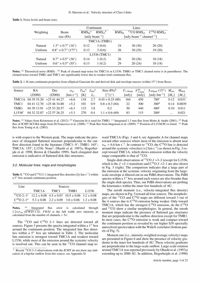
Table 1. Noise levels and beam sizes.
Continuum LinesWeighting Beam RMSth
a RMSclb RMSth
13CO RMScl C18O RMScl
size (PA) [mJy beam−1] [mJy beam−1 channel−1]TMC1A (TMR1)
Natural 1.3′′ × 0.7′′ (16) 0.12 3 (0.6) 24 30 (30) 20 (20)Uniform 0.8′′ × 0.7′′ (177) 0.13 3 (0.6) 26 30 (29) 19 (20)
L1536 (TMC1)Natural 0.7′′ × 0.5′′ (36) 0.14 1 (0.2) 26 20 (26) 18 (18)Uniform 0.6′′ × 0.5′′ (55) 0.13 1 (0.2) 29 20 (24) 18 (18)
Notes. (a) Theoretical noise (RMS) . (b) Peak of cleaned map noise for TMC1A or L1536. TMR1 or TMC1 cleaned noise is in parentheses. Thecleaned noise toward TMR1 and TMC1 are significantly lower due to weaker total continuum flux.
Table 2. 1.36 mm continuum properties from elliptical Gaussian fits and derived disk and envelope masses (within 15′′) from fluxes.
Source RA Dec υlsr Tbola Lbol
a Size (PA)b F1.36mm S int1.3mm
c S 850µm (15′′) Menv Mdisk
(J2000) (J2000) [km s−1] [K] L [′′] () [mJy] [mJy] [mJy bm−1] [M] [M]TMC1A 04 39 35.20 +25 41 44.27 +6.6 118 2.7 0.45 × 0.25 (80) 164 450 780e 0.12 0.033TMC1 04 41 12.70 +25 46 34.80 +5.2 101 0.9 0.8 × 0.3 (84) 22 300 380d 0.14 0.0039TMR1 04 39 13.91 +25 53 20.57 +6.3 133 3.8 0.2 50 440 480e 0.10 0.011L1536f 04 32 32.07 +22 57 26.25 +5.3 270 0.4 1.1 × 0.6 (69) 83 115 200g ... 0.021
Notes. (a) Values from Kristensen et al. (2012). (b) Gaussian fit is used for TMR1. (c) Integrated 1.3 mm flux from Motte & André (2001). (d) Peakflux of JCMT SCUBA maps from Di Francesco et al. (2008). (e) Peak flux from Jørgensen et al. (2009). (f) Position of L1536(W) is listed. (g) Peakflux from Young et al. (2003).
is with respect to the Western peak. The maps indicate the pres-ence of elongated flattened structure perpendicular to the out-flow direction found in the literature (TMC1: 0; TMR1: 165;TMC1A: 155; L1536: None2, Ohashi et al. 1997a; Hogerhei-jde et al. 1998; Brown & Chandler 1999). Such elongated dustemission is indicative of flattened disk-like structures.
3.2. Molecular lines: maps and morphologies
Table 3. 13CO and C18O 2–1 integrated flux densities [Jy km s−1] withina 5′′ box around continuum position.
Line SourcesTMC1A TMC1 TMR1 L1536
13CO 2–1a 12.2 ± 0.08 4.5 ± 0.07 10.5 ± 0.06 3.2 ± 0.08C18O 2–1a 5.3 ± 0.08 2.2 ± 0.09 3.0 ± 0.06 1.2 ± 0.08
Notes. (a) Integrated flux error is calculated through1.2×σrms
√FWZI × δυ. FWZI is the full width zero intensity as
calculated from the number of channels > 5σ.
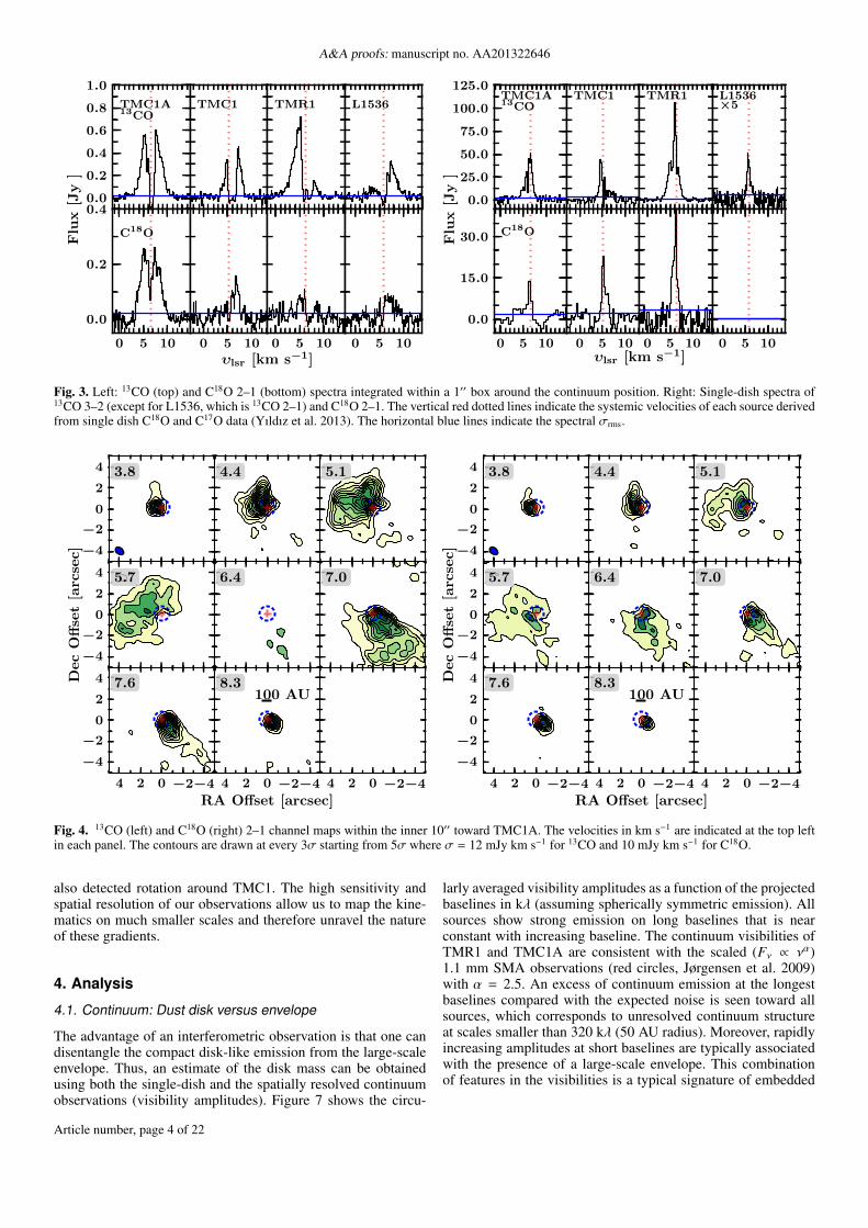
The 13CO and C18O 2–1 lines are detected toward allsources. Figure 3 presents the spectra integrated within a 1′′ boxaround the continuum position. The integrated line flux densi-ties within a 5′′ box are tabulated in Table 3. The molecularline emission is strongest toward TMC1A and weakest towardL1536, while most of the emission around the systemic velocityis resolved out. This can be seen in the 13CO channel map to-2 Recent 12CO 3–2 observations with the JCMT do not show any indi-cation of a bipolar outflow from this source, see Appendix D.
ward TMC1A (Figs. 3 and 4, see Appendix A for channel mapstoward other sources) where most of the emission is absent nearυlsr = 6.6 km s−1. In contrast to 13CO, the C18O line is detectedaround the systemic velocities (±2 km s−1) as shown in Fig. 3 ex-cept toward TMC1A, which shows emission within the velocityrange comparable to that of 13CO.
Single-dish observations of 13CO J =3–2 (except for L1536,which is the J =2–1 transition) and C18O J =2–1 are also shownin Fig. 3 (right). The comparison indicates that a large part ofthe emission at the systemic velocity originating from the large-scale envelope is filtered out in our PdBI observations. The PdBIspectra within a 1′′ box around each source are also broader thanthe single-dish spectra. Thus, our PdBI observations are probingthe kinematics within the inner few hundreds of AU.
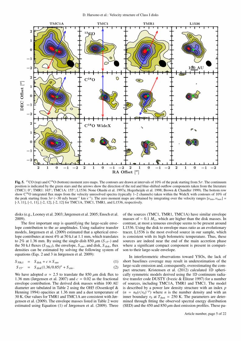
The zeroth moment (i.e., velocity-integrated flux density)maps, are shown in Fig. 5 toward all four sources. The morpholo-gies of the 13CO and C18O maps are different toward 3 out ofthe 4 sources due to C18O emission being weaker. Only towardTMC1A, which has the strongest C18O emission, do the C18Oand 13CO show a similar morphologies. In general, the zerothmoment maps indicate the presence of flattened gas structuresthat are perpendicular to the outflow direction except for TMR1.In most cases, the C18O emission is weak and compact towardthe continuum position as revealed by our higher S/N spectrallyunresolved spectra taken with the WideX correlator (bottom pan-els of Fig. 5).
Moment one (i.e., intensity-weighted average velocity) mapsare presented in Figure 6 and show the presence of velocity gra-dients in the inner few hundreds of AU. These velocity gradientsare perpendicular to the large-scale outflow. Large-scale rotationaround TMC1A was reported previously by Ohashi et al. (1997a)extending up to 2000 AU. In addition, Hogerheijde et al. (1998)
Article number, page 3 of 22
A&A proofs: manuscript no. AA201322646
0.0
0.2
0.4
0.6
0.8
1.0
TMC1A13CO
0 5 10
0.0
0.2
0.4
Flu
x[J
y]
C18O
TMC1
0 5 10
υlsr [km s−1]
TMR1
0 5 10
L1536
0 5 10
0.0
25.0
50.0
75.0
100.0
125.0TMC1A13CO
0 5 10
0.0
15.0
30.0Flu
x[J
y]
C18O
TMC1
0 5 10υlsr [km s−1]
TMR1
0 5 10
L1536×5
0 5 10
Fig. 3. Left: 13CO (top) and C18O 2–1 (bottom) spectra integrated within a 1′′ box around the continuum position. Right: Single-dish spectra of13CO 3–2 (except for L1536, which is 13CO 2–1) and C18O 2–1. The vertical red dotted lines indicate the systemic velocities of each source derivedfrom single dish C18O and C17O data (Yıldız et al. 2013). The horizontal blue lines indicate the spectral σrms.
−4
−2
0
2
4 3.8 4.4 5.1
−4
−2
0
2
4 5.7 6.4 7.0
−4−2024
RA Offset [arcsec]
−4
−2
0
2
4Dec
Off
set
[arc
sec]
7.6
−4−2024
8.3100 AU
−4−2024
−4
−2
0
2
4 3.8 4.4 5.1
−4
−2
0
2
4 5.7 6.4 7.0
−4−2024
RA Offset [arcsec]
−4
−2
0
2
4Dec
Off
set
[arc
sec]
7.6
−4−2024
8.3100 AU
−4−2024
Fig. 4. 13CO (left) and C18O (right) 2–1 channel maps within the inner 10′′ toward TMC1A. The velocities in km s−1 are indicated at the top leftin each panel. The contours are drawn at every 3σ starting from 5σ where σ = 12 mJy km s−1 for 13CO and 10 mJy km s−1 for C18O.
also detected rotation around TMC1. The high sensitivity andspatial resolution of our observations allow us to map the kine-matics on much smaller scales and therefore unravel the natureof these gradients.
4. Analysis
4.1. Continuum: Dust disk versus envelope
The advantage of an interferometric observation is that one candisentangle the compact disk-like emission from the large-scaleenvelope. Thus, an estimate of the disk mass can be obtainedusing both the single-dish and the spatially resolved continuumobservations (visibility amplitudes). Figure 7 shows the circu-
larly averaged visibility amplitudes as a function of the projectedbaselines in kλ (assuming spherically symmetric emission). Allsources show strong emission on long baselines that is nearconstant with increasing baseline. The continuum visibilities ofTMR1 and TMC1A are consistent with the scaled (Fν ∝ να)1.1 mm SMA observations (red circles, Jørgensen et al. 2009)with α = 2.5. An excess of continuum emission at the longestbaselines compared with the expected noise is seen toward allsources, which corresponds to unresolved continuum structureat scales smaller than 320 kλ (50 AU radius). Moreover, rapidlyincreasing amplitudes at short baselines are typically associatedwith the presence of a large-scale envelope. This combinationof features in the visibilities is a typical signature of embedded
Article number, page 4 of 22
D. Harsono et al.: Velocity structure of Class I disks
−2
−1
0
1
2
TMC1A
−2
−1
0
1
2
DE
CO
ffse
t[′′ ]
−2−1012
−2
−1
0
1
2
13CO
TMC1
C18O
−2−1012
C18O WideX
TMR1
−2−1012
RA Offset [′′]
100 AU
L1536
−2−1012
Fig. 5. 13CO (top) and C18O (bottom) moment zero maps. The contours are drawn at intervals of 10% of the peak starting from 5σ. The continuumposition is indicated by the green stars and the arrows show the direction of the red and blue-shifted outflow components taken from the literature(TMC1: 0; TMR1: 165; TMC1A: 155; L1536: None Ohashi et al. 1997a; Hogerheijde et al. 1998; Brown & Chandler 1999). The bottom rowshow C18O integrated flux maps from the velocity unresolved spectra (typically 1–2 channels) taken within the WideX with contours of 10% ofthe peak starting from 3σ (∼30 mJy beam−1 km s−1). The zero moment maps are obtained by integrating over the velocity ranges [υmin, υmax] =[-3, 11], [-1, 11], [-2, 12], [-2, 12] for TMC1A, TMC1, TMR1, and L1536, respectively.
disks (e.g., Looney et al. 2003; Jørgensen et al. 2005; Enoch et al.2009).
The first important step is quantifying the large-scale enve-lope contribution to the uv amplitudes. Using radiative transfermodels, Jørgensen et al. (2009) estimated that a spherical enve-lope contributes at most 4% at 50 kλ at 1.1 mm, which translatesto 2% at 1.36 mm. By using the single-dish 850 µm (S 15′′ ) andthe 50 kλ fluxes (S 50kλ), the envelope, S env, and disk, S disk, fluxdensities can be estimated by solving the following system ofequations (Eqs. 2 and 3 in Jørgensen et al. 2009):
S 50kλ = S disk + c × S env (1)S 15′′ = S disk(1.36/0.85)α + S env. (2)
We have adopted α ' 2.5 to translate the 850 µm disk flux to1.36 mm (Jørgensen et al. 2007) and c = 0.02 as the fractionalenvelope contribution. The derived disk masses within 100 AUdiameter are tabulated in Table 2 using the OH5 (Ossenkopf &Henning 1994) opacities at 1.36 mm and a dust temperature of30 K. Our values for TMR1 and TMC1A are consistent with Jør-gensen et al. (2009). The envelope masses listed in Table 2 wereestimated using Equation (1) of Jørgensen et al. (2009). Three
of the sources (TMC1, TMR1, TMC1A) have similar envelopemasses of ∼ 0.1 M, which are higher than the disk masses. Incontrast, at most a tenuous envelope seems to be present aroundL1536. Using the disk to envelope mass ratio as an evolutionarytracer, L1536 is the most evolved source in our sample, whichis consistent with its high bolometric temperature. Thus, thesesources are indeed near the end of the main accretion phasewhere a significant compact component is present in compari-son to their large-scale envelope.
In interferometric observations toward YSOs, the lack ofshort baselines coverage may result in underestimation of thelarge-scale emission and, consequently, overestimating the com-pact structure. Kristensen et al. (2012) calculated 1D spheri-cally symmetric models derived using the 1D continuum radia-tive transfer code DUSTY (Ivezic & Elitzur 1997) for a numberof sources, including TMC1A, TMR1 and TMC1. The modelis described by a power law density structure with an index p(n = n0(r/r0)−p) where n is the number density and with aninner boundary r0 at Tdust = 250 K. The parameters are deter-mined through fitting the observed spectral energy distribution(SED) and the 450 and 850 µm dust emission profiles. These pa-
Article number, page 5 of 22
A&A proofs: manuscript no. AA201322646
−2−1012
−2
−1
0
1
213CO
TMC1A
−2−1012RA Offset [′′]
−2
−1
0
1
2
DE
CO
ffse
t[′′ ]
C18O
−2−1012
100 AU
TMC1
−2−1012
−2−1012
TMR1
−2−1012
−2−1012
L1536
−2−1012
5
6
7
8
5
6
7
8
4
5
6
7
4
5
6
7
4
5
6
5
6
4
6
8
4
6
8
υls
r[k
ms−
1]
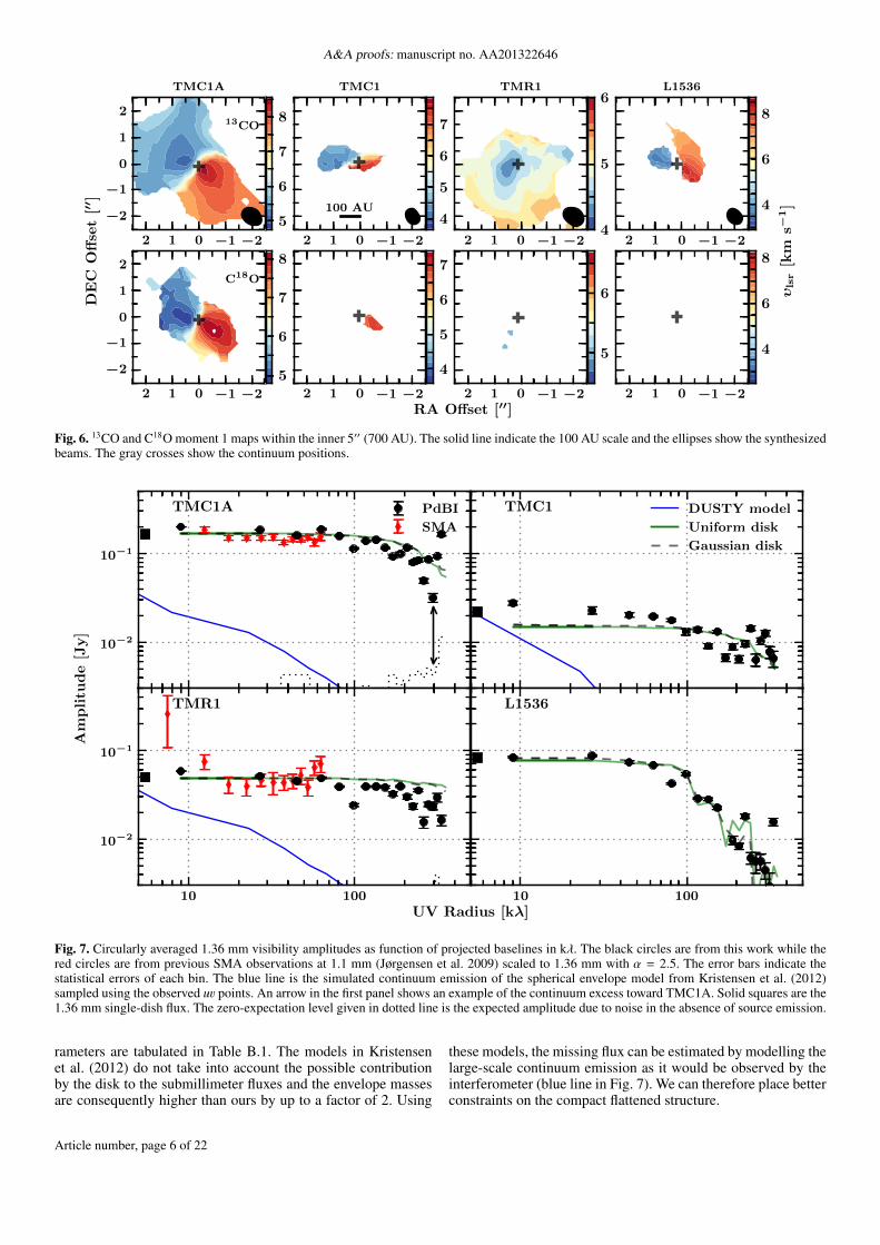
Fig. 6. 13CO and C18O moment 1 maps within the inner 5′′ (700 AU). The solid line indicate the 100 AU scale and the ellipses show the synthesizedbeams. The gray crosses show the continuum positions.
10−2
10−1
TMC1A PdBI
SMA
TMC1 DUSTY model
Uniform disk
Gaussian disk
10 100UV Radius [kλ]
10−2
10−1
Am
pli
tud
e[J
y]
TMR1
10 100
L1536
Fig. 7. Circularly averaged 1.36 mm visibility amplitudes as function of projected baselines in kλ. The black circles are from this work while thered circles are from previous SMA observations at 1.1 mm (Jørgensen et al. 2009) scaled to 1.36 mm with α = 2.5. The error bars indicate thestatistical errors of each bin. The blue line is the simulated continuum emission of the spherical envelope model from Kristensen et al. (2012)sampled using the observed uv points. An arrow in the first panel shows an example of the continuum excess toward TMC1A. Solid squares are the1.36 mm single-dish flux. The zero-expectation level given in dotted line is the expected amplitude due to noise in the absence of source emission.
rameters are tabulated in Table B.1. The models in Kristensenet al. (2012) do not take into account the possible contributionby the disk to the submillimeter fluxes and the envelope massesare consequently higher than ours by up to a factor of 2. Using
these models, the missing flux can be estimated by modelling thelarge-scale continuum emission as it would be observed by theinterferometer (blue line in Fig. 7). We can therefore place betterconstraints on the compact flattened structure.
Article number, page 6 of 22

D. Harsono et al.: Velocity structure of Class I disks
−2
−1
0
1
2 TMC1A
70 AU
TMC1
−2−1012
RA Offset [′′]
−2
−1
0
1
2
DE
CO
ffse
t[′′ ]
TMR1
−2−1012
L1536
Fig. 1. 1.36 mm uniform weighted continuum maps toward TMC1A(I4365+2535, top left), TMC1 (I4381+2540, top right), TMR1(I4361+2547, bottom left), and L1536 (I4295+2251, bottom right). Thecontours start from 10σ up to 80σ by 10σ. The peak flux densities perbeam are 11 mJy, 42 mJy, 23 mJy and 128 mJy for TMC1, TMR1,L1536 and TMC1A, respectively. The red circles indicate the best-fitsource-position assuming elliptical Gaussian while the black ellipsesshow the synthesized beams. The arrows indicate the outflow direction.The RMS is given in Table 1. The dashed blue lines indicate the negativecontours starting at 3σ.
−1.0−0.50.00.51.0
RA Offset [′′]
−1.0
−0.5
0.0
0.5
1.0
DE
CO
ffse
t[′′ ]
70 AU
L1536
Fig. 2. Zoom of the continuum image toward L1536. Both of the lineand color contours are drawn at 10% of the peak starting from 4σ upto the peak intensity of 23 mJy beam−1, while the synthesized beam isindicated by the black ellipse in the bottom right corner.
4.2. Constraining the dust disk parameters
The goal of this section is to estimate the size and mass of thecompact flattened dust structure or the disk using a number of
Table 4. Disk sizes and masses derived from continuum visibilitiesmodelling using uniform, Gaussian and power-law disk models.
Object ParametersRdisk Mdisk i PA[AU] [10−3 M] [] []
Uniform diskTMC1A 30 – 50 48±6 20–46 60–99TMC1 7 – 124 4.7+4
−2 30–70 65–105TMR1 7 – 40 15±2 5–30 -15–15L1536 100 – 171 22±5 30–73 60–100
Gaussian diskTMC1A 17–32 48±6 24–56 62–96TMC1 7–80 4.5+4
−2 30–70 65–105TMR1 7–20 15±2 5–30 -15–15L1536 53–112 24±4 33–75 60–100
Power-law diskTMC1A 80–220 41±8 24–76 60–99TMC1 41–300 5.4+20
−0 20–80 55–115TMR1 7–55 10+100
−9 2–45 -25–40L1536 135–300 19+18
−4 20–56 50–68
0.0
0.2
0.4
0.6
0.8
1.0
0.5
0.8
1.0
Un
iform
70
140
210 AU
0.0
0.2
0.4
0.6
0.8
1.0
Norm
ali
zedI(r
)
0.5
0.8
1.0N
orm
ali
zed
Am
pli
tud
e
Gau
ssian41
110
221 AU
0.0 0.5 1.0 1.5 2.0
r [arcsec]
0.0
0.2
0.4
0.6
0.8
1.0
1 10 100
UV radius [kλ]
0.5
0.8
1.0 Pow
er
law
500
326
107
47 AU
Fig. 8. Left: Normalized intensity profiles for the three different contin-uum models: Uniform disk (top), Gaussian Disk (middle), and power-law disk (bottom). Right: Normalized visibilities as function of uv ra-dius. For comparison, the L1536 binned data are shown in gray circles.
more sophisticated methods than Eq. (1) and (2) to compare withthe estimates from the gas in the next section. We define the diskcomponent to be any compact flattened structure that deviatesfrom the expected continuum emission due to the spherical en-velope model. In the following sections, the disk sizes will beestimated by fitting the continuum visibilities with the inclusionof emission from the large-scale structure described above. Asthe interferometric observation recovers a large fraction of thesingle-dish flux toward L1536, its large-scale envelope contribu-
Article number, page 7 of 22
A&A proofs: manuscript no. AA201322646
tion is assumed to be insignificant, and therefore not included.The best-fit parameters are found through χ2 minimization onthe binned amplitudes. The range of values of Rdisk, Mdisk, i andPA shown in Table 4 correspond to models with χ2 between χ2
minand χ2
min + 15.
4.2.1. Uniform disk
The first estimate on the disk size and mass is obtained by fittinga uniform disk model assuming optically thin dust emission (seeFig. 8, Eisner 2012). Uniform disks are described by a constantintensity I within a diameter θud whose flux is given by F =∫
I cos θ dΩ = Iπ(θud2
)2. The visibility amplitudes are given by:
V(u, v) = F × 2J1 (πθruv)πθruv
, (3)
where J1 is the Bessel function of order 1 and ruv is the projectedbaseline in terms of λ. Deprojection of the baselines follow theformula given in Berger & Segransan (2007):
uPA = u cos PA + v sin PA, (4)vPA = −u sin PA + v cos PA, (5)
ruv,i =
√(u2
PA + v2PA cos(i)2), (6)
where PA is the position angle (East of North) and i is the incli-nation.
The best fit parameters are tabulated in Table 4 with diskmasses estimated using a dust temperature of 30 K and OH5opacities (Table 5 of Ossenkopf & Henning 1994) within θud
2 ra-dius. The disk radii vary between 7 to 171 AU. The smallest disksize is found toward TMR1, which suggests that most of its con-tinuum emission is due to the large-scale envelope. Moreover,disk sizes around TMR1 and TMC1A are 65%–90% lower thanthose reported by Eisner (2012, Table 3) since we have includedthe spherical envelope contribution. This illustrates the impor-tance of including the large-scale contribution in analyzing thecompact structure.
4.2.2. Gaussian disk
The next step is to use a Gaussian intensity distribution, which isa slightly more realistic intensity model that represents the mmemission due to an embedded disk. The visibility amplitudes aredescribed by the following equation:
V(u, v) = F × exp(−πθGruv
4 log 2
), (7)
where θG is the FWHM of the Gaussian distribution and F is thetotal flux.
The difference between the Gaussian fit presented in Table 2and this section is the inclusion of the large-scale emission. InTable 2, the Gaussian fit gives an estimate of the size of emissionin the observed total image, while this section accounts for thesimulated large-scale envelope emission in order to constrain thecompact flattened structure. The free-parameters are similar tothe uniform disk except that the size of the emitting region isdefined by full-width half maximum (FWHM). For a Gaussiandistribution, most of the radiation (95%) is emitted from within2σG ∼ 0.85×FWHM, thus we define the disk radius to be 0.42×FWHM. The best-fit parameters are tabulated in Table 4 and thecorresponding emission is included in Fig. 7. The resulting disksizes are slightly lower than those derived using a uniform disk.
The visibility amplitudes in Fig. 7 show the presence of anunresolved point source component at long baselines indicatedby the arrow in the first panel. Jørgensen et al. (2005) notedthat a three components model (large-scale envelope + Gaus-sian disk + point-source) fits the continuum visibilities. By usingsuch models, the disk sizes generally increase by 20–30 AU withthe addition of an unresolved point flux, which is comparable tothe uniform disk models. Such models were first introduced byMundy et al. (1996) since the mm emission seems to be morecentrally peaked than a single Gaussian. The unresolved pointflux is more likely due to the unresolved disk structure sincethe free-free emission contribution is expected to be low towardClass I sources (Hogerheijde et al. 1998).
4.2.3. Power-law disk
The next step in sophistication is to fit the continuum visibilitieswith a power-law disk structure. The difference is that the firsttwo disk models are based on the expected intensity profile ofthe disk, while the power-law disk models use a more realisticdisk structure. Similar structures were previously used by Layet al. (1997, see also Lay et al. 1994; Mundy et al. 1996; Dutreyet al. 2007; Malbet et al. 2005). We adopt a disk density struc-ture described by Σdisk = Σ50AU (R/50AU)−p where Σ50 AU is thesurface density at 50 AU with a temperature structure given asTdisk = 1500 (R/0.1AU)−q. The inner radius is fixed at 0.1 AUwith a dust sublimation temperature of 1500 K, while the diskouter radius is defined at 15 K. The free parameters are p, q,Σ50AU, i and PA where i is the inclination with respect of theplane of the sky in degrees (0 is face-on) and PA is the positionangle (East of North). The visibilities are constructed by consid-ering the flux from a thin ring given by:
dS =2π cos i
d2 Bν(T )(1 − exp−τ
)R dR, (8)
where d is the distance, i is the inclination (0 is face-on), τ =Σ(R)κcos i is the optical depth and Bν(T ) is the Planck function. For thedust emissivity (κ), we adopt the OH5 values. Since the modelis axisymmetric, the visibilities are given by a one-dimensionalHankel transform which is given by the analytical expression:
V (u, v) = dS × J0 (2πRruv) , (9)
where J0 is the Bessel function of order 0. The total amplitudeat a given ruv is integrated over the whole disk.
The first advantage of such modelling is the treatment of theoptical depth which gives better mass approximations. Secondly,the unresolved point-flux is already included in the model bysimulating the emission from the unresolved disk component.Figure 8 shows the normalized visibilities for a fixed p = 0.9and a number of Rdisk. The best-fit parameters are tabulated inTable 4.
The derived disk masses obtained by integrating out to ∼ 50AU radius are similar to those from the 50 kλ point (Table 2).This is expected as the 1.3 mm continuum emission (κOH5 =0.83 cm2g−1) is on average nearly optically thin (Jørgensen et al.2007). The optical depth can be up to 0.4 at radii < 10 AU forthe best-fit power-law disk models with i > 70. A wide rangeof ‘best-fit’ masses is found toward TMR1, which is mainly dueto the uncertainties in the inclination.
More recently, Eisner (2012) presented embedded disk mod-els derived from continuum data by fitting the I band image,SED and 1.3 mm visibilities. Our continuum disk radii towardTMC1A and TMR1 are consistent with their results. However,
Article number, page 8 of 22

D. Harsono et al.: Velocity structure of Class I disks
the high quality of our data allow us to rule out disks withRout > 100 AU toward TMR1. On the other hand, our disk radiustoward L1536 is a factor of 3 higher than that reported in Eisner(2012) due to the difference in the treatment of the large-scaleenvelope.
In summary, different methods have been used to constrainthe disk parameters from thermal dust emission. The first twomodels, Gaussian and uniform disk models, are based on the in-tensity profile, while the power-law disk models use a simpli-fied disk structure with given density and temperature profiles.The intensity based models find the smallest disk sizes, whilethe power-law disk models predict up to a factor of two largerdisk sizes. On the other hand, the disk masses from these fittingmethods are similar. The advantage of the power-law disk mod-eling is the determination of the density and temperature struc-tures including the unresolved inner part of the disk. The contin-uum images provide no kinematic information, however, so theimportant question is whether these flattened structures are rota-tionally supported disks and if so, whether the continuum sizesagree with those of RSDs.
4.3. Line analysis: Keplerian or not?
The nature of the velocity gradient can already be inferred fromthe moment maps. First, the 13CO integrated flux maps shownin Fig. 5 indicate the presence of flattened gas structures perpen-dicular to the outflow direction. Second, the velocity gradientis also oriented perpendicular to the outflow within hundreds ofAU, which is a similar size scale to the compact dust structuremeasured in Section 4.2. On the other hand, the velocity gradientdoes not show a straight transition from the red to the blue shiftedcomponent as expected from a Keplerian disk. Taking TMC1Aas an example, the blue-shifted emission starts at the North sideand skews inward toward the continuum position. Such a skewedmoment 1 map is expected for a Keplerian disk embedded in arotating infalling envelope (Sargent & Beckwith 1987; Brinchet al. 2008). Thus, the moment maps indicate the presence of arotating infalling envelope leading up to a rotationally dominatedstructure.
In image space, position velocity (PV) diagrams are gener-ally used to determine the nature of the velocity gradient. Anal-ysis of such diagrams starts by dividing it into four quadrantsaround the υlsr and source position. A rotating structure occupiestwo of the four quadrants that are symmetric around the center,while an infalling structure will show emission in all quadrants(e.g., Ohashi et al. 1997a; Brinch et al. 2007). In addition, onecan infer the presence of outflow contamination by identifying avelocity gradient in PV space along the outflow direction (e.g.,Cabrit et al. 1996).
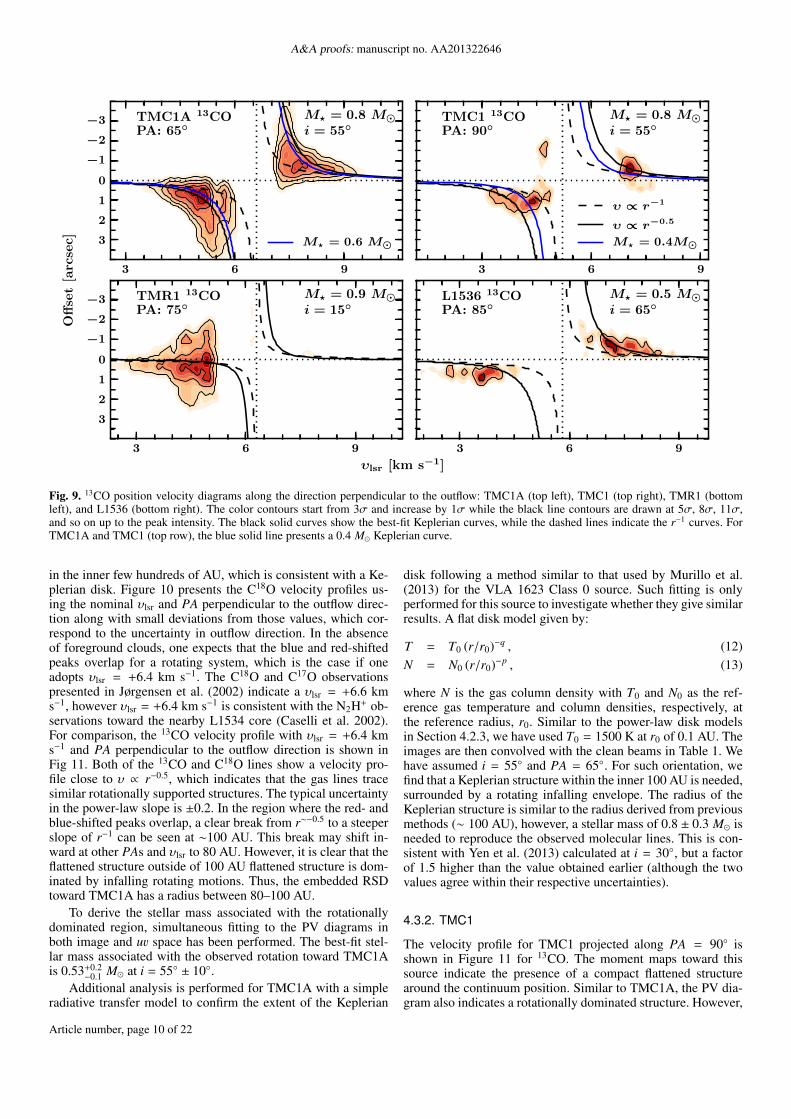
Figure 9 presents PV diagrams at a direction perpendicularto the outflow direction; for L1536, the direction of elongation ofthe continuum was taken. In general, the PV diagrams are con-sistent with Keplerian profiles, except for TMR1. The PV dia-gram toward TMR1 seems to indicate that the 13CO line is eitherdominated by infalling material or the source is oriented towardus, which is difficult to disentangle. However, recent 12CO 3–2and 6–5 maps presented in Yıldız et al, (in prep.) suggest that thedisk is more likely oriented face-on (i < 15). Furthermore, a ve-locity gradient is present in the 13CO PV analysis both along andperpendicular to the outflow direction indicating minor outflowcontamination for this source.
The focus of this paper is to differentiate between the in-falling gas and the rotationally supported disk. Such analysis inimage space is not sensitive to the point where the infalling ro-
tating material (υ ∝ r−1) enters the disk and becomes Keplerian(υ ∝ r−0.5). Thus, additional analysis is needed to differentiatebetween the two cases.
As pointed out by Lin et al. (1994), infalling gas that con-serves its angular momentum exhibits a steeper velocity profile(υ ∝ r−1) than free-falling gas (υ ∝ r−0.5). In the case of spec-trally resolved optically thin lines, the peak position of the emis-sion corresponds to the maximum possible position of the emit-ting gas (Sargent & Beckwith 1987; Harsono et al. 2013). Onthe other hand, molecular emission closer to the systemic veloc-ity is optically thick and, consequently, the inferred positions areonly lower limits. Thus, with such a method, one can differen-tiate between the Keplerian disk and the infalling rotating gas.Moreover, Harsono et al. (2013) suggested that the point wherethe two velocity profiles meet corresponds to the size of the Ke-plerian disk, Rk. In the following sections, we will attempt toconstrain the size of the Keplerian disk using this method, whichwe will term the uv-space PV diagram.
The peak positions are determined by fitting the velocity re-solved visibilities with Gaussian functions (Lommen et al. 2008;Jørgensen et al. 2009). It can be seen from the channel maps(Fig. 4 and Appendix A) that a Gaussian brightness distributionis a good approximation in determining the peak positions of thehigh velocity channels.
To characterize the profile of the velocity gradient, the peakpositions are projected along the velocity gradient. This is doneby using the following transformation
xPA = x cos(PA) + y sin(PA), (10)yPA = −x sin(PA) + y cos(PA), (11)
where x, y are the peak positions and xθ, yθ are the rotated posi-tions. A velocity profile (υ ∝ r−η) is then fitted to a subset of thered- and blue-shifted peaks to determine the best velocity profile.
4.3.1. TMC1A
1
2
3υlsr = 6.4
PA = 55
30 50 100R [AU]
1
2
3
∆υ
(υ−υ
lsr)
[km
s−1]
υlsr = 6.6
PA = 55
υlsr = 6.4
PA = 65
30 50 100
υlsr = 6.6
PA = 65
Fig. 10. C18O uv-space PV diagrams toward TMC1A with PA =55, 65 and υlsr = 6.6, 6.4 km s−1. The solid lines are the r−0.5 curvesand dashed lines are the r−1 curves. The red and blue colors indicate thered- and blue-shifted components, respectively. Gray points show therest of the peaks that were not included in the fitting.
TMC1A shows the greatest promise so far for an embeddedKeplerian disk around a Class I protostar . The moment 1 maps(Fig. 6) indicate a gradual change from blue- to red-shifted gas
Article number, page 9 of 22
A&A proofs: manuscript no. AA201322646
3 6 9
−3
−2
−1
0
1
2
3
TMC1A 13COPA: 65
M? = 0.8 Mi = 55
M? = 0.6 M
3 6 9
TMC1 13COPA: 90
M? = 0.8 Mi = 55
υ ∝ r−1
υ ∝ r−0.5
M? = 0.4M
3 6 9
υlsr [km s−1]
−3
−2
−1
0
1
2
3
Off
set
[arc
sec]
TMR1 13COPA: 75
M? = 0.9 Mi = 15
3 6 9
L1536 13COPA: 85
M? = 0.5 Mi = 65
Fig. 9. 13CO position velocity diagrams along the direction perpendicular to the outflow: TMC1A (top left), TMC1 (top right), TMR1 (bottomleft), and L1536 (bottom right). The color contours start from 3σ and increase by 1σ while the black line contours are drawn at 5σ, 8σ, 11σ,and so on up to the peak intensity. The black solid curves show the best-fit Keplerian curves, while the dashed lines indicate the r−1 curves. ForTMC1A and TMC1 (top row), the blue solid line presents a 0.4 M Keplerian curve.
in the inner few hundreds of AU, which is consistent with a Ke-plerian disk. Figure 10 presents the C18O velocity profiles us-ing the nominal υlsr and PA perpendicular to the outflow direc-tion along with small deviations from those values, which cor-respond to the uncertainty in outflow direction. In the absenceof foreground clouds, one expects that the blue and red-shiftedpeaks overlap for a rotating system, which is the case if oneadopts υlsr = +6.4 km s−1. The C18O and C17O observationspresented in Jørgensen et al. (2002) indicate a υlsr = +6.6 kms−1, however υlsr = +6.4 km s−1 is consistent with the N2H+ ob-servations toward the nearby L1534 core (Caselli et al. 2002).For comparison, the 13CO velocity profile with υlsr = +6.4 kms−1 and PA perpendicular to the outflow direction is shown inFig 11. Both of the 13CO and C18O lines show a velocity pro-file close to υ ∝ r−0.5, which indicates that the gas lines tracesimilar rotationally supported structures. The typical uncertaintyin the power-law slope is ±0.2. In the region where the red- andblue-shifted peaks overlap, a clear break from r∼−0.5 to a steeperslope of r−1 can be seen at ∼100 AU. This break may shift in-ward at other PAs and υlsr to 80 AU. However, it is clear that theflattened structure outside of 100 AU flattened structure is dom-inated by infalling rotating motions. Thus, the embedded RSDtoward TMC1A has a radius between 80–100 AU.
To derive the stellar mass associated with the rotationallydominated region, simultaneous fitting to the PV diagrams inboth image and uv space has been performed. The best-fit stel-lar mass associated with the observed rotation toward TMC1Ais 0.53+0.2
−0.1 M at i = 55 ± 10.Additional analysis is performed for TMC1A with a simple
radiative transfer model to confirm the extent of the Keplerian
disk following a method similar to that used by Murillo et al.(2013) for the VLA 1623 Class 0 source. Such fitting is onlyperformed for this source to investigate whether they give similarresults. A flat disk model given by:
T = T0 (r/r0)−q , (12)N = N0 (r/r0)−p , (13)
where N is the gas column density with T0 and N0 as the ref-erence gas temperature and column densities, respectively, atthe reference radius, r0. Similar to the power-law disk modelsin Section 4.2.3, we have used T0 = 1500 K at r0 of 0.1 AU. Theimages are then convolved with the clean beams in Table 1. Wehave assumed i = 55 and PA = 65. For such orientation, wefind that a Keplerian structure within the inner 100 AU is needed,surrounded by a rotating infalling envelope. The radius of theKeplerian structure is similar to the radius derived from previousmethods (∼ 100 AU), however, a stellar mass of 0.8 ± 0.3 M isneeded to reproduce the observed molecular lines. This is con-sistent with Yen et al. (2013) calculated at i = 30, but a factorof 1.5 higher than the value obtained earlier (although the twovalues agree within their respective uncertainties).
4.3.2. TMC1
The velocity profile for TMC1 projected along PA = 90 isshown in Figure 11 for 13CO. The moment maps toward thissource indicate the presence of a compact flattened structurearound the continuum position. Similar to TMC1A, the PV dia-gram also indicates a rotationally dominated structure. However,
Article number, page 10 of 22
D. Harsono et al.: Velocity structure of Class I disks
2
3
TMC1A13COυlsr = 6.4 km s−1
PA = 65
r−0.5TMC113COυlsr = 5.2
PA = 89
r−0.9
25 50 100R [AU]
2
3
∆υ
(υ−υ
lsr)
[km
s−1]
TMR113COυlsr = 6.3
PA = 75
r−0.5
r−1.0
25 50 100
L153613COυlsr = 5.3
PA = 85
r−0.5
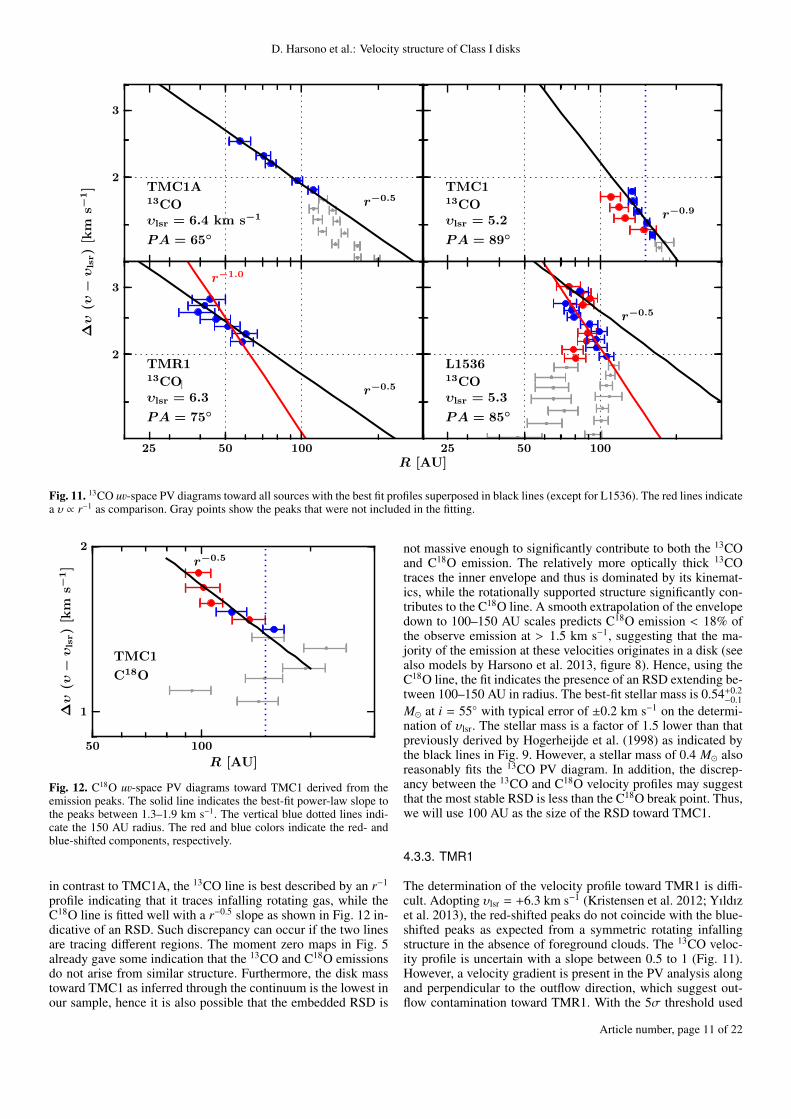
Fig. 11. 13CO uv-space PV diagrams toward all sources with the best fit profiles superposed in black lines (except for L1536). The red lines indicatea υ ∝ r−1 as comparison. Gray points show the peaks that were not included in the fitting.
50 100
R [AU]
1
2
∆υ
(υ−υ
lsr)
[km
s−1]
TMC1
C18O
r−0.5
Fig. 12. C18O uv-space PV diagrams toward TMC1 derived from theemission peaks. The solid line indicates the best-fit power-law slope tothe peaks between 1.3–1.9 km s−1. The vertical blue dotted lines indi-cate the 150 AU radius. The red and blue colors indicate the red- andblue-shifted components, respectively.
in contrast to TMC1A, the 13CO line is best described by an r−1
profile indicating that it traces infalling rotating gas, while theC18O line is fitted well with a r−0.5 slope as shown in Fig. 12 in-dicative of an RSD. Such discrepancy can occur if the two linesare tracing different regions. The moment zero maps in Fig. 5already gave some indication that the 13CO and C18O emissionsdo not arise from similar structure. Furthermore, the disk masstoward TMC1 as inferred through the continuum is the lowest inour sample, hence it is also possible that the embedded RSD is
not massive enough to significantly contribute to both the 13COand C18O emission. The relatively more optically thick 13COtraces the inner envelope and thus is dominated by its kinemat-ics, while the rotationally supported structure significantly con-tributes to the C18O line. A smooth extrapolation of the envelopedown to 100–150 AU scales predicts C18O emission < 18% ofthe observe emission at > 1.5 km s−1, suggesting that the ma-jority of the emission at these velocities originates in a disk (seealso models by Harsono et al. 2013, figure 8). Hence, using theC18O line, the fit indicates the presence of an RSD extending be-tween 100–150 AU in radius. The best-fit stellar mass is 0.54+0.2
−0.1M at i = 55 with typical error of ±0.2 km s−1 on the determi-nation of υlsr. The stellar mass is a factor of 1.5 lower than thatpreviously derived by Hogerheijde et al. (1998) as indicated bythe black lines in Fig. 9. However, a stellar mass of 0.4 M alsoreasonably fits the 13CO PV diagram. In addition, the discrep-ancy between the 13CO and C18O velocity profiles may suggestthat the most stable RSD is less than the C18O break point. Thus,we will use 100 AU as the size of the RSD toward TMC1.
4.3.3. TMR1
The determination of the velocity profile toward TMR1 is diffi-cult. Adopting υlsr = +6.3 km s−1 (Kristensen et al. 2012; Yıldızet al. 2013), the red-shifted peaks do not coincide with the blue-shifted peaks as expected from a symmetric rotating infallingstructure in the absence of foreground clouds. The 13CO veloc-ity profile is uncertain with a slope between 0.5 to 1 (Fig. 11).However, a velocity gradient is present in the PV analysis alongand perpendicular to the outflow direction, which suggest out-flow contamination toward TMR1. With the 5σ threshold used
Article number, page 11 of 22
A&A proofs: manuscript no. AA201322646
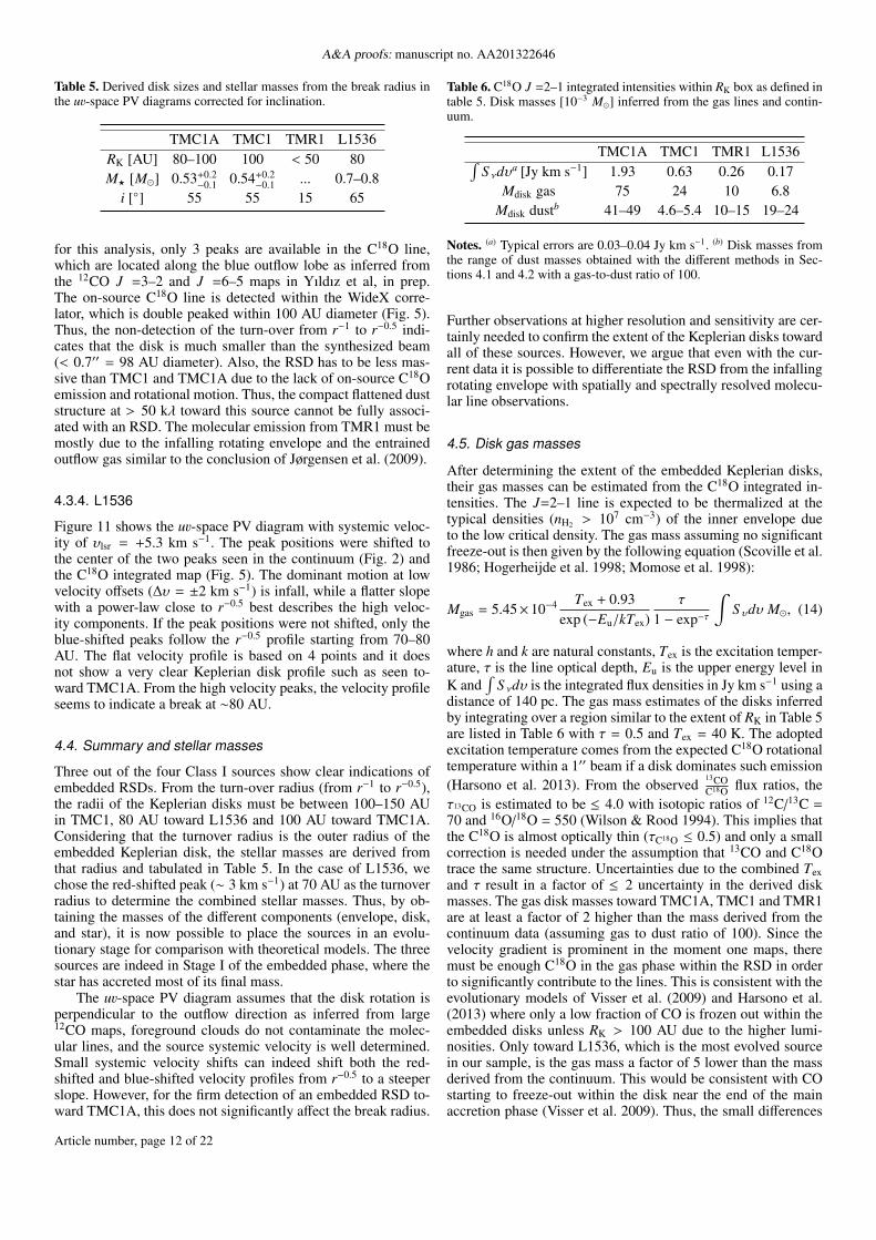
Table 5. Derived disk sizes and stellar masses from the break radius inthe uv-space PV diagrams corrected for inclination.
TMC1A TMC1 TMR1 L1536RK [AU] 80–100 100 < 50 80M? [M] 0.53+0.2
−0.1 0.54+0.2−0.1 ... 0.7–0.8
i [] 55 55 15 65
for this analysis, only 3 peaks are available in the C18O line,which are located along the blue outflow lobe as inferred fromthe 12CO J =3–2 and J =6–5 maps in Yıldız et al, in prep.The on-source C18O line is detected within the WideX corre-lator, which is double peaked within 100 AU diameter (Fig. 5).Thus, the non-detection of the turn-over from r−1 to r−0.5 indi-cates that the disk is much smaller than the synthesized beam(< 0.7′′ = 98 AU diameter). Also, the RSD has to be less mas-sive than TMC1 and TMC1A due to the lack of on-source C18Oemission and rotational motion. Thus, the compact flattened duststructure at > 50 kλ toward this source cannot be fully associ-ated with an RSD. The molecular emission from TMR1 must bemostly due to the infalling rotating envelope and the entrainedoutflow gas similar to the conclusion of Jørgensen et al. (2009).
4.3.4. L1536
Figure 11 shows the uv-space PV diagram with systemic veloc-ity of υlsr = +5.3 km s−1. The peak positions were shifted tothe center of the two peaks seen in the continuum (Fig. 2) andthe C18O integrated map (Fig. 5). The dominant motion at lowvelocity offsets (∆υ = ±2 km s−1) is infall, while a flatter slopewith a power-law close to r−0.5 best describes the high veloc-ity components. If the peak positions were not shifted, only theblue-shifted peaks follow the r−0.5 profile starting from 70–80AU. The flat velocity profile is based on 4 points and it doesnot show a very clear Keplerian disk profile such as seen to-ward TMC1A. From the high velocity peaks, the velocity profileseems to indicate a break at ∼80 AU.
4.4. Summary and stellar masses
Three out of the four Class I sources show clear indications ofembedded RSDs. From the turn-over radius (from r−1 to r−0.5),the radii of the Keplerian disks must be between 100–150 AUin TMC1, 80 AU toward L1536 and 100 AU toward TMC1A.Considering that the turnover radius is the outer radius of theembedded Keplerian disk, the stellar masses are derived fromthat radius and tabulated in Table 5. In the case of L1536, wechose the red-shifted peak (∼ 3 km s−1) at 70 AU as the turnoverradius to determine the combined stellar masses. Thus, by ob-taining the masses of the different components (envelope, disk,and star), it is now possible to place the sources in an evolu-tionary stage for comparison with theoretical models. The threesources are indeed in Stage I of the embedded phase, where thestar has accreted most of its final mass.
The uv-space PV diagram assumes that the disk rotation isperpendicular to the outflow direction as inferred from large12CO maps, foreground clouds do not contaminate the molec-ular lines, and the source systemic velocity is well determined.Small systemic velocity shifts can indeed shift both the red-shifted and blue-shifted velocity profiles from r−0.5 to a steeperslope. However, for the firm detection of an embedded RSD to-ward TMC1A, this does not significantly affect the break radius.
Table 6. C18O J =2–1 integrated intensities within RK box as defined intable 5. Disk masses [10−3 M] inferred from the gas lines and contin-uum.
TMC1A TMC1 TMR1 L1536∫S νdυa [Jy km s−1] 1.93 0.63 0.26 0.17
Mdisk gas 75 24 10 6.8Mdisk dustb 41–49 4.6–5.4 10–15 19–24
Notes. (a) Typical errors are 0.03–0.04 Jy km s−1. (b) Disk masses fromthe range of dust masses obtained with the different methods in Sec-tions 4.1 and 4.2 with a gas-to-dust ratio of 100.
Further observations at higher resolution and sensitivity are cer-tainly needed to confirm the extent of the Keplerian disks towardall of these sources. However, we argue that even with the cur-rent data it is possible to differentiate the RSD from the infallingrotating envelope with spatially and spectrally resolved molecu-lar line observations.
4.5. Disk gas masses
After determining the extent of the embedded Keplerian disks,their gas masses can be estimated from the C18O integrated in-tensities. The J=2–1 line is expected to be thermalized at thetypical densities (nH2 > 107 cm−3) of the inner envelope dueto the low critical density. The gas mass assuming no significantfreeze-out is then given by the following equation (Scoville et al.1986; Hogerheijde et al. 1998; Momose et al. 1998):
Mgas = 5.45×10⁻⁴ Tex + 0.93exp (−Eu/kTex)
τ
1 − exp−τ
∫S υdυ M, (14)
where h and k are natural constants, Tex is the excitation temper-ature, τ is the line optical depth, Eu is the upper energy level inK and
∫S νdυ is the integrated flux densities in Jy km s−1 using a
distance of 140 pc. The gas mass estimates of the disks inferredby integrating over a region similar to the extent of RK in Table 5are listed in Table 6 with τ = 0.5 and Tex = 40 K. The adoptedexcitation temperature comes from the expected C18O rotationaltemperature within a 1′′ beam if a disk dominates such emission(Harsono et al. 2013). From the observed
13COC18O flux ratios, the
τ13CO is estimated to be ≤ 4.0 with isotopic ratios of 12C/13C =70 and 16O/18O = 550 (Wilson & Rood 1994). This implies thatthe C18O is almost optically thin (τC18O ≤ 0.5) and only a smallcorrection is needed under the assumption that 13CO and C18Otrace the same structure. Uncertainties due to the combined Texand τ result in a factor of ≤ 2 uncertainty in the derived diskmasses. The gas disk masses toward TMC1A, TMC1 and TMR1are at least a factor of 2 higher than the mass derived from thecontinuum data (assuming gas to dust ratio of 100). Since thevelocity gradient is prominent in the moment one maps, theremust be enough C18O in the gas phase within the RSD in orderto significantly contribute to the lines. This is consistent with theevolutionary models of Visser et al. (2009) and Harsono et al.(2013) where only a low fraction of CO is frozen out within theembedded disks unless RK > 100 AU due to the higher lumi-nosities. Only toward L1536, which is the most evolved sourcein our sample, is the gas mass a factor of 5 lower than the massderived from the continuum. This would be consistent with COstarting to freeze-out within the disk near the end of the mainaccretion phase (Visser et al. 2009). Thus, the small differences
Article number, page 12 of 22
D. Harsono et al.: Velocity structure of Class I disks
between gas and dust masses indicate relatively low CO freeze-out in embedded disks.
5. Discussion
5.1. Disk structure comparison: dust versus gas
In this paper, we have determined the sizes of the disk-like struc-tures around Class I embedded YSOs using both the continuumand the gas lines. The continuum analysis focuses on the extentof continuum emission excluding the large-scale emission, whilethe gas line analysis focuses on placing constraint on the size ofthe RSD. The continuum analysis utilizes both intensity baseddisk models and a simple disk structure (power-law disk model).The intensity based disk models give a large spread of disk radiitoward all sources. On the other other hand, the best-fit radii ofpower-law disks are larger than the Keplerian disk toward TMR1and L1536, while the values are comparable toward TMC1A andTMC1. Not all of the disk structure derived from continuum ob-servations may be associated to an RSD.
The main caveat in deriving the flattened disk structure fromcontinuum visibilities is the estimate of the large-scale envelopeemission. It has been previously shown that the large-scale enve-lope can deviate from spherical symmetry (e.g., Looney et al.2007; Tobin et al. 2010). Disk structures may change if oneadopts a 2D flattened envelope structure due to the mass distribu-tion at 50–300 AU scale. However, in this paper, we focused onthe size of the flattened structure where any deviation from thespherically symmetry model gives an estimate of its size. For thepurpose of this paper, a spherical envelope model is used to esti-mate the large-scale envelope contribution since it is simple, fitsthe observed visibilities at short baselines, and does not requireadditional parameters.
5.1.1. Comparison to disk sizes and masses from SEDmodelling
A number of 2D envelope and disk models have been publishedpreviously constrained solely using continuum data. More re-cently, Eisner (2012) used the combination of high resolutionnear-IR images, the SED and millimeter continuum visibilitiesto constrain the structures around TMR1, TMC1A and L1536.The size of his disk is defined by the centrifugal radius, whichis the radius at which the material distribution becomes moreflattened (Ulrich 1976). His inferred sizes are consistent withthe extent of RSDs in our sample (TMR1: 30–450 AU; L1536:30–100 AU; TMC1A: 100 AU), but our higher resolution datanarrow this range. For the case of TMR1, we can definitely ruleout any disk sizes > 100 AU.
Others have used a similar definition of the centrifugal radiususing the envelope structure given by Ulrich (1976) with andwithout disk component (e.g., Eisner et al. 2005; Gramajo et al.2007; Furlan et al. 2008). Thus, the value of Rc gives an approxi-mate outer radius of the RSD. These models are then fitted to theSED and high resolution near-IR images without interferometricdata. In general, the values of Rc derived from such models arelower (at least by factor of 2) than the extent of the RSDs as in-dicated by our molecular line observations. By trying to fit themodels to the near-IR images which are dominated by the hotdust within the disk, they put more weight to the inner region.Thus, we argue that spatially resolved millimeter data are neces-sary in order to place better constraints on the compact flattenedstructure.
0.0 0.2 0.4 0.6 0.8 1.0
M?/Mtot
0
50
100
150
200
250
300
350
400
RK
[AU
]
Ω = 10−14, cs = 0.26
Ω = 10−14, cs = 0.19
Ω = 10−13, cs = 0.26N1333I4A2
L1527
VLA1623
IRS7B
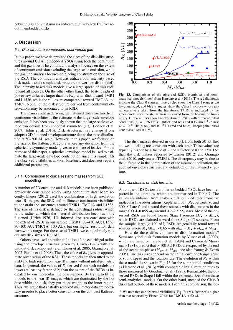
Fig. 13. Comparison of the observed RSDs (symbols) and semi-analytical models (lines) from Harsono et al. (2013). The red diamondsindicate the Class 0 sources, blue circles show the Class I sources wehave analyzed, and blue triangles show the Class I sources whose pa-rameters were taken from the literatures. TMR1 is indicated by thegreen circle since the stellar mass is derived from the bolometric lumi-nosity. Different lines show the evolution of RSDs with different initialconditions (cs = 0.26 km s−1 (black and red) and 0.19 km s−1 (blue);Ω = 10−13 Hz (black) and 10−14 Hz (red and blue)), keeping the initialcore mass fixed at 1 M.
The disk masses derived in our work from both 50 kλ fluxand uvmodelling are consistent with each other. These values aretypically higher by a factor of 2 and a factor of 8 for TMC1A3
than the disk masses reported by Eisner (2012) and Gramajoet al. (2010, only toward TMR1). The discrepancy may be due tothe difference in the combination of the assumed inclination, theadopted envelope structure, and definition of the flattened struc-ture.
5.2. Constraints on disk formation
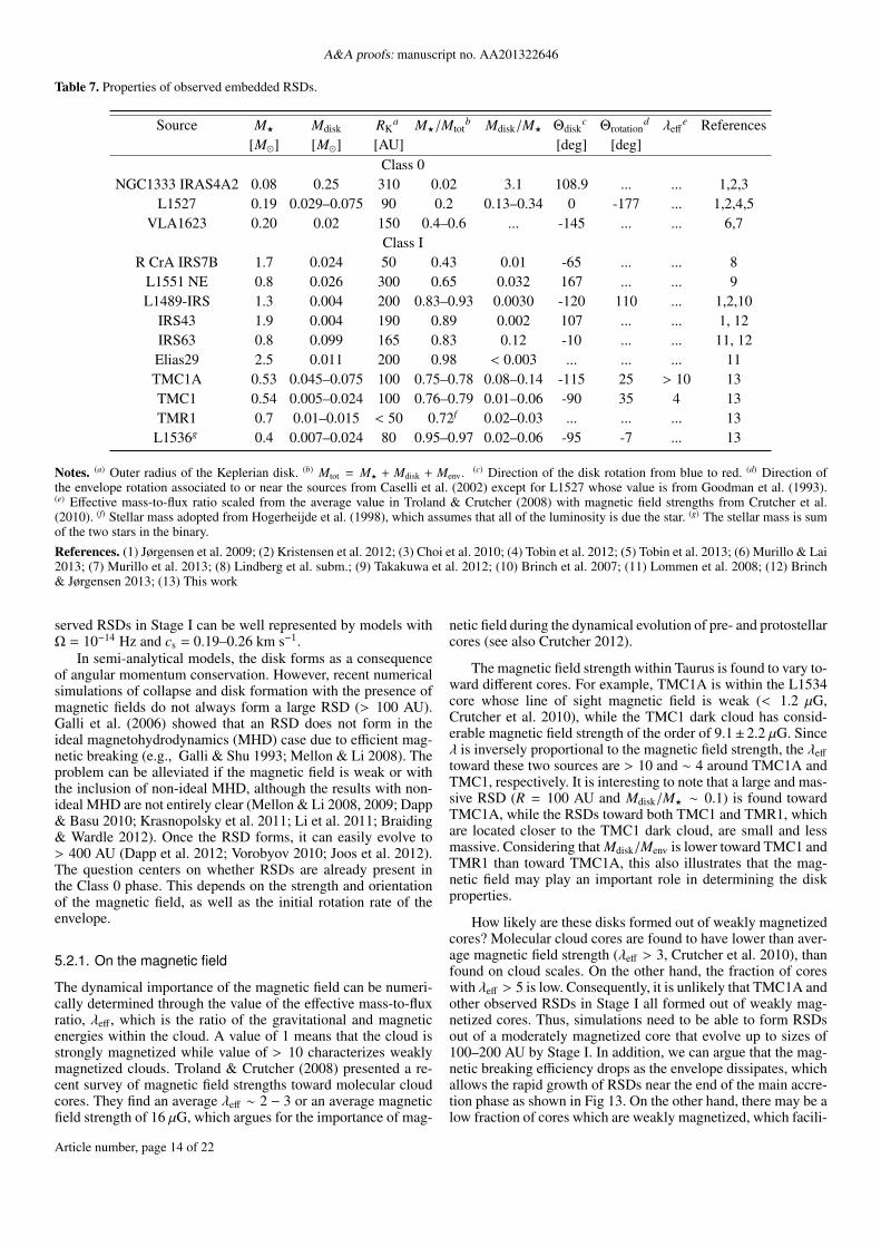
A number of RSDs toward other embedded YSOs have been re-ported in the literature, which are summarized in Table 7. Thevalues are obtained from analysis that included interferometricmolecular line observations. Keplerian radii, RK, between 80 and300 AU are found toward these sources with disk masses in therange 0.004–0.055 M around 0.2–2.5 M stars. Most of the ob-served RSDs are found toward Stage I sources (M? > Menv),while RSDs are claimed toward three Stage 0/I sources. Fromthe sample, large (≥ 100 AU) RSDs are generally found towardsources where M?/Mtot > 0.65 with Mtot = M? + Menv + Mdisk.
How do these disks compare to disk formation models?Semi-analytical disk formation models by Visser et al. (2009),which are based on Terebey et al. (1984) and Cassen & Moos-man (1981), predict that > 100 AU RSDs are expected by the endof the accretion phase (Menv < Mdisk, see also Young & Evans2005). The disk sizes depend on the initial envelope temperatureor sound speed and the rotation rate. The evolution of RK withinthese models is shown in Fig. 13 for the same initial conditionsas Harsono et al. (2013) with comparable initial rotation rates tothose measured by Goodman et al. (1993). Remarkably, the ob-served RSDs in Stage I fall within the expected sizes from thesesemi-analytical models. On the other hand, most of the Class 0disks fall outside of these models. From this comparison, the ob-
3 We note that our observed visibilities (Fig. 7) are a factor of 3 higherthan that reported by Eisner (2012) for TMC1A at 50 kλ.
Article number, page 13 of 22
A&A proofs: manuscript no. AA201322646
Table 7. Properties of observed embedded RSDs.
Source M? Mdisk RKa M?/Mtot
b Mdisk/M? Θdiskc Θrotation
d λeffe References
[M] [M] [AU] [deg] [deg]Class 0
NGC1333 IRAS4A2 0.08 0.25 310 0.02 3.1 108.9 ... ... 1,2,3L1527 0.19 0.029–0.075 90 0.2 0.13–0.34 0 -177 ... 1,2,4,5
VLA1623 0.20 0.02 150 0.4–0.6 ... -145 ... ... 6,7Class I
R CrA IRS7B 1.7 0.024 50 0.43 0.01 -65 ... ... 8L1551 NE 0.8 0.026 300 0.65 0.032 167 ... ... 9L1489-IRS 1.3 0.004 200 0.83–0.93 0.0030 -120 110 ... 1,2,10
IRS43 1.9 0.004 190 0.89 0.002 107 ... ... 1, 12IRS63 0.8 0.099 165 0.83 0.12 -10 ... ... 11, 12Elias29 2.5 0.011 200 0.98 < 0.003 ... ... ... 11TMC1A 0.53 0.045–0.075 100 0.75–0.78 0.08–0.14 -115 25 > 10 13TMC1 0.54 0.005–0.024 100 0.76–0.79 0.01–0.06 -90 35 4 13TMR1 0.7 0.01–0.015 < 50 0.72f 0.02–0.03 ... ... ... 13
L1536g 0.4 0.007–0.024 80 0.95–0.97 0.02–0.06 -95 -7 ... 13
Notes. (a) Outer radius of the Keplerian disk. (b) Mtot = M? + Mdisk + Menv. (c) Direction of the disk rotation from blue to red. (d) Direction ofthe envelope rotation associated to or near the sources from Caselli et al. (2002) except for L1527 whose value is from Goodman et al. (1993).(e) Effective mass-to-flux ratio scaled from the average value in Troland & Crutcher (2008) with magnetic field strengths from Crutcher et al.(2010). (f) Stellar mass adopted from Hogerheijde et al. (1998), which assumes that all of the luminosity is due the star. (g) The stellar mass is sumof the two stars in the binary.
References. (1) Jørgensen et al. 2009; (2) Kristensen et al. 2012; (3) Choi et al. 2010; (4) Tobin et al. 2012; (5) Tobin et al. 2013; (6) Murillo & Lai2013; (7) Murillo et al. 2013; (8) Lindberg et al. subm.; (9) Takakuwa et al. 2012; (10) Brinch et al. 2007; (11) Lommen et al. 2008; (12) Brinch& Jørgensen 2013; (13) This work
served RSDs in Stage I can be well represented by models withΩ = 10−14 Hz and cs = 0.19–0.26 km s−1.
In semi-analytical models, the disk forms as a consequenceof angular momentum conservation. However, recent numericalsimulations of collapse and disk formation with the presence ofmagnetic fields do not always form a large RSD (> 100 AU).Galli et al. (2006) showed that an RSD does not form in theideal magnetohydrodynamics (MHD) case due to efficient mag-netic breaking (e.g., Galli & Shu 1993; Mellon & Li 2008). Theproblem can be alleviated if the magnetic field is weak or withthe inclusion of non-ideal MHD, although the results with non-ideal MHD are not entirely clear (Mellon & Li 2008, 2009; Dapp& Basu 2010; Krasnopolsky et al. 2011; Li et al. 2011; Braiding& Wardle 2012). Once the RSD forms, it can easily evolve to> 400 AU (Dapp et al. 2012; Vorobyov 2010; Joos et al. 2012).The question centers on whether RSDs are already present inthe Class 0 phase. This depends on the strength and orientationof the magnetic field, as well as the initial rotation rate of theenvelope.
5.2.1. On the magnetic field
The dynamical importance of the magnetic field can be numeri-cally determined through the value of the effective mass-to-fluxratio, λeff , which is the ratio of the gravitational and magneticenergies within the cloud. A value of 1 means that the cloud isstrongly magnetized while value of > 10 characterizes weaklymagnetized clouds. Troland & Crutcher (2008) presented a re-cent survey of magnetic field strengths toward molecular cloudcores. They find an average λeff ∼ 2 − 3 or an average magneticfield strength of 16 µG, which argues for the importance of mag-
netic field during the dynamical evolution of pre- and protostellarcores (see also Crutcher 2012).
The magnetic field strength within Taurus is found to vary to-ward different cores. For example, TMC1A is within the L1534core whose line of sight magnetic field is weak (< 1.2 µG,Crutcher et al. 2010), while the TMC1 dark cloud has consid-erable magnetic field strength of the order of 9.1± 2.2 µG. Sinceλ is inversely proportional to the magnetic field strength, the λeff
toward these two sources are > 10 and ∼ 4 around TMC1A andTMC1, respectively. It is interesting to note that a large and mas-sive RSD (R = 100 AU and Mdisk/M? ∼ 0.1) is found towardTMC1A, while the RSDs toward both TMC1 and TMR1, whichare located closer to the TMC1 dark cloud, are small and lessmassive. Considering that Mdisk/Menv is lower toward TMC1 andTMR1 than toward TMC1A, this also illustrates that the mag-netic field may play an important role in determining the diskproperties.
How likely are these disks formed out of weakly magnetizedcores? Molecular cloud cores are found to have lower than aver-age magnetic field strength (λeff > 3, Crutcher et al. 2010), thanfound on cloud scales. On the other hand, the fraction of coreswith λeff > 5 is low. Consequently, it is unlikely that TMC1A andother observed RSDs in Stage I all formed out of weakly mag-netized cores. Thus, simulations need to be able to form RSDsout of a moderately magnetized core that evolve up to sizes of100–200 AU by Stage I. In addition, we can argue that the mag-netic breaking efficiency drops as the envelope dissipates, whichallows the rapid growth of RSDs near the end of the main accre-tion phase as shown in Fig 13. On the other hand, there may be alow fraction of cores which are weakly magnetized, which facili-
Article number, page 14 of 22
D. Harsono et al.: Velocity structure of Class I disks
tate formation of large disks as early as Stage 0 phase (Krumholzet al. 2013; Murillo et al. 2013).
5.2.2. On the large-scale rotation
Another important parameter is the large-scale rotation aroundthese sources, which is a parameter used in both simulations andsemi-analytical models. Generally, a cloud rotation rate between10−14 Hz to a few 10−13 Hz is used in numerical simulations(e.g., Yorke & Bodenheimer 1999; Li et al. 2011). The aver-age rotation rate measured by Goodman et al. (1993) is ∼ 10−14
Hz, which is consistent with the initial rotation rate of the semi-analytical model that best describes a large fraction of the ob-served RSDs. The time at which Stage I starts within that modelis 3×10⁵ years. For comparison, around the same computationaltime, Yorke & Bodenheimer (1999) form a > 500 AU RSD fortheir low-mass case (J). Similarly, Vorobyov (2010) also found> 200 AU RSDs close to the start of the Class II phase. We findno evidence of such large RSDs at similar evolutionary stages inour observations.
Another aspect of the large-scale rotation that is worth inves-tigating is its direction with respect to that of the disk rotation.Models assume that the disk rotation direction is the same as therotation of its core. To compare the directions, we have used thevelocity gradients reported by Caselli et al. (2002) and Good-man et al. (1993) toward the dark cores in Taurus. Velocity gra-dients are detected toward L1534 (TMC1A), L1536 and TMC-1C, which is located to the North East of TMR1 and TMC1.Table 7 lists the velocity gradients of the RSDs toward the em-bedded objects and their envelope/core rotation4. It is interestingto note that the large-scale rotation detected around or nearbythe RSDs have a different velocity gradient direction. Similarmisalignments in rotation have been pointed out by Takakuwaet al. (2012) toward L1551 NE and by Tobin et al. (2013) forL1527. Although the positions of the detected molecular emis-sion in Caselli et al. (2002) do not necessarily coincide with theembedded objects due to chemical effects, the systematic veloc-ities of the cores are similar. Misalignment at 1000 AU scaleswas also concluded by Brinch et al. (2007) toward L1489 wherethey found that the Keplerian disk and the rotating envelope areat an angle of 30 with respect to each other. If these objectsformed out of these cores in the distant past, then either the col-lapse process changed the angular momentum of the envelopeand, consequently, the disk rotation direction or it affects the an-gular momentum distribution of nearby cores through feedback.Interestingly, the former may suggest the importance of the non-ideal MHD effect called the Hall effect during disk formation,which can produce counter-rotating disks (Li et al. 2011; Braid-ing & Wardle 2012).
Finally, the simulations and models above require the initialcore to be rotating in order to form RSDs. However, by analyzingthe angular momentum distribution of magnetized cores, Dzibet al. (2010) suggested that the NH3 and N2H+ measurementsmay overestimate the angular momentum by a factor of ∼ 8−10.This poses further problems to disk formation in previous numer-ical studies of collapse and disk formation. On the other hand,the inclusion of the Hall effect does not require a rotating enve-lope core to form a rotating structure (e.g., Krasnopolsky et al.2011; Li et al. 2011). Further studies are required to compare theexpected observables from rotating and non-rotating models.
4 The direction is in degrees East of North and increasing υlsr (blueto red) to be consistent with Caselli et al. (2002) and Goodman et al.(1993).
5.3. Disk stability
Self gravitating disks can be important during the early stages ofstar formation in regulating the accretion process onto the pro-tostar, which can be variable (e.g., Vorobyov 2010). Dunham &Vorobyov (2012) show that such episodic accretion events canreproduce the observed population of YSOs. A self-gravitatingdisk is expected when Mdisk/Mstar ≥ 0.1 (e.g., Lodato & Rice2004; Boley et al. 2006; Cossins et al. 2009). However, most ofthe observed embedded RSDs around Class I sources have diskmasses such that Mdisk/Mstar ≤ 0.1. It is unlikely for such disksto become self-gravitating, but they may have been in the past.Interestingly, a few embedded disk seem to be self-gravitatingsince their Mdisk/Mstar ≥ 0.1 such as toward TMC1A, IRS63,L1527 and NGC1333 IRAS4A2 (See Table 7).
The low fraction of large and massive disks during the em-bedded phase suggests that disk instabilities may have takenplace in the past and limited their current observed numbers(i.e. low fluxes at long baselines). In this scenario, the embed-ded disks will have a faster evolution and, thus, spend most oftheir lifetime with small radii. Alternatively, disks experienc-ing high infall rates from envelope to the disk as expected dur-ing the embedded phase may also have higher accretion rates(Harsono et al. 2011). Such a scenario argues for disk instabil-ities to be present even for Mdisk/M? < 0.1. In both cases, thedominant motion of the compact flattened structure during theembedded phase is infall rather than rotation. There are indeedsources where higher sensitivity and spatial resolution observa-tions such as with Atacama Large Millimeter/submillimeter Ar-ray (ALMA) can detect features associated with disk instabili-ties (e.g., Cossins et al. 2010; Forgan et al. 2012; Douglas et al.2013).
6. Conclusions
We present spatially and spectrally resolved observations downto a radius of 56 AU around four Class I YSOs in Taurus. TheC18O and 13CO 2–1 lines are used to differentiate the infallingrotating envelope from the rotationally supported disk. Analysisof the dust and gas lines were performed directly in uv space toavoid any artefacts introduced during the inversion process. Themain results of this paper are:
– Dust disk sizes and masses can be derived from the contin-uum by using a power-law spherical envelope model to ac-count for the large-scale envelope emission. Intensity baseddisk models (Uniform and Gaussian) give similar disk sizesto each other which are lower by typically 25%-90% thanrealistic disk models (power-law disk). On the other hand,they give similar disk masses to more realistic models, whichare consistent with the disk mass derived from the 50 kλflux point. Inclusion of the envelope in the analysis is im-portant to obtain reliable disk masses. The observationallyderived masses indicate that there is still a significant enve-lope present toward three of the four sources: TM1A, TMC1,and TMR1.
– Three of the four sources (TMC1, L1536, TMC1A) hostembedded rotationally supported disks (RSDs) derived fromline data. By fitting velocity profiles (υ ∝ r−0.5 or ∝ r−1.0)to the red- and blue-shifted peaks, the RSDs are found tohave outer radii of ∼ 80–100 AU. In addition, the large-scalestructure (> 100 AU) is dominated by the infalling rotat-ing envelope (υ ∝ r−1). The derived stellar masses of thesesources are of order 0.4–0.8 M, consistent with previous
Article number, page 15 of 22
A&A proofs: manuscript no. AA201322646
values. Consequently, these objects are indeed Stage I youngstellar objects with M?/(Menv + Mdisk + M?) > 0.7.
– Disk radii derived from the power-law dust disk models to-ward TMC1 and TMC1A are consistent with sizes of theirRSDs. However, the dust disk radii toward TMR1 and L1536are not the same as the extent of their RSDs. Thus, we em-phasize that spatially and spectrally resolved gas lines obser-vations are required to study the nature of flattened structurestoward embedded YSOs.
– Semi-analytical models with Ω = 10−14 Hz and cs = 0.19 –0.26 km s−1describe most of the observed RSDs in Stage I.The observed RSDs argue for inefficient magnetic breakingnear the end of the main accretion phase (M?/Mtot > 0.65).More theoretical studies are needed to understand how andwhen RSDs form under such conditions.
– Comparison between disk masses derived from the contin-uum and C18O integrated line intensities (Table 6) suggeststhat relatively little of CO is frozen out within the embeddeddisk.
The current constraints on disk formation rely on a smallnumber of observed RSDs around Class I sources. Certainly oneneeds to constrain the size of RSDs near the end of the mainaccretion phase to understand how late Class II disks form. Onthe other hand, the observed RSDs in the Class I phase do notanswer the question when and how RSDs form. Such constraintsrequire the detection and characterization of RSDs during Class0 phase, which are currently lacking. From the sample of sourcesin Yen et al. (2013) and our results, it is clear that the infallingrotating flattened structure is present at >100 AU. Thus, extend-ing molecular line observations down to < 50 AU radius withALMA toward Class 0 YSOs will be crucial for differentiatingbetween the different scenarios for disk formation.
Acknowledgements
We thank the anonymous referee for the constructive com-ments. We are grateful to the IRAM staff, in particular toChin-Shin Chang, Tessel van der Laan and Jérôme Pety, fortheir help with the observations, reduction and modelling ofthe data. We thank Umut Yıldız for reducing the single-dishdata and making them available. This work is supported by theNetherlands Research School for Astronomy (NOVA) and bythe Space Research Organization Netherlands (SRON). Astro-chemistry in Leiden is supported by the Netherlands ResearchSchool for Astronomy (NOVA), by a Spinoza grant and grant614.001.008 from the Netherlands Organisation for ScientificResearch (NWO), and by the European Community’s SeventhFramework Programme FP7/2007–2013 under grant agreement238258 (LASSIE). This research was supported by a LundbeckFoundation Group Leader Fellowship to Jes Jørgensen. Researchat Centre for Star and Planet Formation is funded by the Dan-ish National Research Foundation and the University of Copen-hagen’s programme of excellence. This research used the facil-ities of the Canadian Astronomy Data Centre operated by theNational Research Council of Canada with the support of theCanadian Space Agency.
ReferencesAikawa, Y., Furuya, K., Wakelam, V., et al. 2011, in IAU Symposium, Vol. 280,
IAU Symposium, ed. J. Cernicharo & R. Bachiller, 33–42Aikawa, Y., Wakelam, V., Garrod, R. T., & Herbst, E. 2008, ApJ, 674, 984Andre, P., Ward-Thompson, D., & Barsony, M. 1993, ApJ, 406, 122
Berger, J. P. & Segransan, D. 2007, New A Rev., 51, 576Bodenheimer, P. 1995, ARA&A, 33, 199Boley, A. C., Mejía, A. C., Durisen, R. H., et al. 2006, ApJ, 651, 517Braiding, C. R. & Wardle, M. 2012, MNRAS, 422, 261Brinch, C., Crapsi, A., Jørgensen, J. K., Hogerheijde, M. R., & Hill, T. 2007,
A&A, 475, 915Brinch, C., Hogerheijde, M. R., & Richling, S. 2008, A&A, 489, 607Brinch, C. & Jørgensen, J. K. 2013, A&A, 559, A82Brown, D. W. & Chandler, C. J. 1999, MNRAS, 303, 855Cabrit, S., Guilloteau, S., Andre, P., et al. 1996, A&A, 305, 527Caselli, P., Benson, P. J., Myers, P. C., & Tafalla, M. 2002, ApJ, 572, 238Cassen, P. & Moosman, A. 1981, Icarus, 48, 353Chiang, H.-F., Looney, L. W., Tassis, K., Mundy, L. G., & Mouschovias, T. C.
2008, ApJ, 680, 474Chiang, H.-F., Looney, L. W., & Tobin, J. J. 2012, ApJ, 756, 168Choi, M., Tatematsu, K., & Kang, M. 2010, ApJ, 723, L34Cossins, P., Lodato, G., & Clarke, C. J. 2009, MNRAS, 393, 1157Cossins, P., Lodato, G., & Testi, L. 2010, MNRAS, 407, 181Crapsi, A., van Dishoeck, E. F., Hogerheijde, M. R., Pontoppidan, K. M., &
Dullemond, C. P. 2008, A&A, 486, 245Crutcher, R. M. 2012, ARA&A, 50, 29Crutcher, R. M., Hakobian, N., & Troland, T. H. 2010, MNRAS, 402, L64Dapp, W. B. & Basu, S. 2010, A&A, 521, L56Dapp, W. B., Basu, S., & Kunz, M. W. 2012, A&A, 541, A35Di Francesco, J., Johnstone, D., Kirk, H., MacKenzie, T., & Ledwosinska, E.
2008, ApJS, 175, 277Douglas, T. A., Caselli, P., Ilee, J. D., et al. 2013, MNRAS, 433, 2064Dunham, M. M., Evans, II, N. J., Terebey, S., Dullemond, C. P., & Young, C. H.
2010, ApJ, 710, 470Dunham, M. M. & Vorobyov, E. I. 2012, ApJ, 747, 52Dutrey, A., Guilloteau, S., & Ho, P. 2007, in Protostars and Planets V, B.
Reipurth, D. Jewitt, and K. Keil (eds.), University of Arizona Press, Tucson,951 pp., 2007., p.495-506 LPI, États-Unis, 495–506
Dzib, S., Loinard, L., Mioduszewski, A. J., et al. 2010, ApJ, 718, 610Eisner, J. A. 2012, ApJ, 755, 23Eisner, J. A., Hillenbrand, L. A., Carpenter, J. M., & Wolf, S. 2005, ApJ, 635,
396Enoch, M. L., Corder, S., Duchêne, G., et al. 2011, ApJS, 195, 21Enoch, M. L., Corder, S., Dunham, M. M., & Duchêne, G. 2009, ApJ, 707, 103Forgan, D., Armitage, P. J., & Simon, J. B. 2012, MNRAS, 426, 2419Furlan, E., McClure, M., Calvet, N., et al. 2008, ApJS, 176, 184Galli, D., Lizano, S., Shu, F. H., & Allen, A. 2006, ApJ, 647, 374Galli, D. & Shu, F. H. 1993, ApJ, 417, 220Goodman, A. A., Benson, P. J., Fuller, G. A., & Myers, P. C. 1993, ApJ, 406,
528Gramajo, L. V., Whitney, B. A., Gómez, M., & Robitaille, T. P. 2010, AJ, 139,
2504Gramajo, L. V., Whitney, B. A., Kenyon, S. J., Gómez, M., & Merrill, K. M.
2007, AJ, 133, 1911Harsono, D., Alexander, R. D., & Levin, Y. 2011, MNRAS, 413, 423Harsono, D., Visser, R., Bruderer, S., van Dishoeck, E. F., & Kristensen, L. E.
2013, A&A, 555, A45Hayashi, M., Ohashi, N., & Miyama, S. M. 1993, ApJ, 418, L71Hogerheijde, M. R., van Dishoeck, E. F., Blake, G. A., & van Langevelde, H. J.
1998, ApJ, 502, 315Ivezic, Z. & Elitzur, M. 1997, MNRAS, 287, 799Joos, M., Hennebelle, P., & Ciardi, A. 2012, A&A, 543, A128Jørgensen, J. K., Bourke, T. L., Myers, P. C., et al. 2007, ApJ, 659, 479Jørgensen, J. K., Bourke, T. L., Myers, P. C., et al. 2005, ApJ, 632, 973Jørgensen, J. K., Schöier, F. L., & van Dishoeck, E. F. 2002, A&A, 389, 908Jørgensen, J. K., van Dishoeck, E. F., Visser, R., et al. 2009, A&A, 507, 861Keene, J. & Masson, C. R. 1990, ApJ, 355, 635Krasnopolsky, R., Li, Z.-Y., & Shang, H. 2011, ApJ, 733, 54Kristensen, L. E., van Dishoeck, E. F., Bergin, E. A., et al. 2012, A&A, 542, A8Krumholz, M. R., Crutcher, R. M., & Hull, C. L. H. 2013, ApJ, 767, L11Lada, C. J. & Wilking, B. A. 1984, ApJ, 287, 610Lay, O. P., Carlstrom, J. E., & Hills, R. E. 1997, ApJ, 489, 917Lay, O. P., Carlstrom, J. E., Hills, R. E., & Phillips, T. G. 1994, ApJ, 434, L75Lee, C.-F. 2010, ApJ, 725, 712Lee, C.-F. 2011, ApJ, 741, 62Li, Z.-Y., Krasnopolsky, R., & Shang, H. 2011, ApJ, 738, 180Lin, D. N. C., Hayashi, M., Bell, K. R., & Ohashi, N. 1994, ApJ, 435, 821Lodato, G. & Rice, W. K. M. 2004, MNRAS, 351, 630Lommen, D., Jørgensen, J. K., van Dishoeck, E. F., & Crapsi, A. 2008, A&A,
481, 141Looney, L. W., Mundy, L. G., & Welch, W. J. 2003, ApJ, 592, 255Looney, L. W., Tobin, J. J., & Kwon, W. 2007, ApJ, 670, L131Malbet, F., Lachaume, R., Berger, J.-P., et al. 2005, A&A, 437, 627Mellon, R. R. & Li, Z.-Y. 2008, ApJ, 681, 1356Mellon, R. R. & Li, Z.-Y. 2009, ApJ, 698, 922
Article number, page 16 of 22
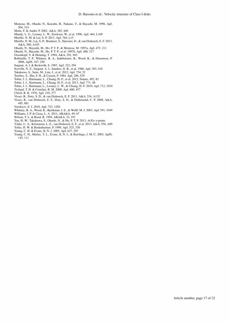
D. Harsono et al.: Velocity structure of Class I disks
Momose, M., Ohashi, N., Kawabe, R., Nakano, T., & Hayashi, M. 1998, ApJ,504, 314
Motte, F. & André, P. 2001, A&A, 365, 440Mundy, L. G., Looney, L. W., Erickson, W., et al. 1996, ApJ, 464, L169Murillo, N. M. & Lai, S.-P. 2013, ApJ, 764, L15Murillo, N. M., Lai, S.-P., Bruderer, S., Harsono, D., & van Dishoeck, E. F. 2013,
A&A, 560, A103Ohashi, N., Hayashi, M., Ho, P. T. P., & Momose, M. 1997a, ApJ, 475, 211Ohashi, N., Hayashi, M., Ho, P. T. P., et al. 1997b, ApJ, 488, 317Ossenkopf, V. & Henning, T. 1994, A&A, 291, 943Robitaille, T. P., Whitney, B. A., Indebetouw, R., Wood, K., & Denzmore, P.
2006, ApJS, 167, 256Sargent, A. I. & Beckwith, S. 1987, ApJ, 323, 294Scoville, N. Z., Sargent, A. I., Sanders, D. B., et al. 1986, ApJ, 303, 416Takakuwa, S., Saito, M., Lim, J., et al. 2012, ApJ, 754, 52Terebey, S., Shu, F. H., & Cassen, P. 1984, ApJ, 286, 529Tobin, J. J., Hartmann, L., Chiang, H.-F., et al. 2012, Nature, 492, 83Tobin, J. J., Hartmann, L., Chiang, H.-F., et al. 2013, ApJ, 771, 48Tobin, J. J., Hartmann, L., Looney, L. W., & Chiang, H.-F. 2010, ApJ, 712, 1010Troland, T. H. & Crutcher, R. M. 2008, ApJ, 680, 457Ulrich, R. K. 1976, ApJ, 210, 377Visser, R., Doty, S. D., & van Dishoeck, E. F. 2011, A&A, 534, A132Visser, R., van Dishoeck, E. F., Doty, S. D., & Dullemond, C. P. 2009, A&A,
495, 881Vorobyov, E. I. 2010, ApJ, 723, 1294Whitney, B. A., Wood, K., Bjorkman, J. E., & Wolff, M. J. 2003, ApJ, 591, 1049Williams, J. P. & Cieza, L. A. 2011, ARA&A, 49, 67Wilson, T. L. & Rood, R. 1994, ARA&A, 32, 191Yen, H.-W., Takakuwa, S., Ohashi, N., & Ho, P. T. P. 2013, ArXiv e-printsYıldız, U. A., Kristensen, L. E., van Dishoeck, E. F., et al. 2013, A&A, 556, A89Yorke, H. W. & Bodenheimer, P. 1999, ApJ, 525, 330Young, C. H. & Evans, II, N. J. 2005, ApJ, 627, 293Young, C. H., Shirley, Y. L., Evans, II, N. J., & Rawlings, J. M. C. 2003, ApJS,
145, 111
Article number, page 17 of 22

A&A–AA201322646, Online Material p 18
−4
−2
0
2
4 3.6 4.1 4.6
−4
−2
0
2
4 5.2 5.7 6.2
−4−2024
RA Offset [arcsec]
−4
−2
0
2
4
Dec
Off
set
[arcse
c]
6.8
−4−2024
7.3100 AU
−4−2024
7.8
Fig. A.1. 13CO 2–1 channel maps similar to Fig. 4 toward TMC1.
−4
−2
0
2
4 3.6 4.1 4.6
−4
−2
0
2
4 5.2 5.7 6.2
−4−2024
RA Offset [arcsec]
−4
−2
0
2
4
Dec
Off
set
[arcse
c]
6.8
−4−2024
7.3100 AU
−4−2024
7.8
Fig. A.2. C18O 2–1 channel maps similar to Fig. 4 toward TMC1.
Appendix A: Observational data
The observational log can be found in Table A.1 and the channelmaps of all the observed lines toward the four sources are shownin Figs. A.1– A.6.
Appendix B: Large-scale structure
The parameters of the large-scale envelope structure used to esti-mate the continuum emission at short baselines are in Table B.1.
−4
−2
0
2
4 2.8 3.4 4.0
−4
−2
0
2
4 4.7 5.3 5.9
−4−2024
RA Offset [arcsec]
−4
−2
0
2
4
Dec
Off
set
[arcse
c]
6.6
−4−2024
7.2100 AU
−4−2024
7.9
Fig. A.3. 13CO 2–1 channel maps similar to Fig. 4 toward TMR1.
−4
−2
0
2
4 2.8 3.4 4.0
−4
−2
0
2
4 4.7 5.3 6.0
−4−2024
RA Offset [arcsec]
−4
−2
0
2
4
Dec
Off
set
[arcse
c]
6.6
−4−2024
7.2100 AU
−4−2024
7.9
Fig. A.4. C18O 2–1 channel maps similar to Fig. 4 toward TMR1.
Table B.1. 1D spherical envelope parameters as published by Kris-tensen et al. (2012).
Source p Ya rin nin n(1000AU)[AU] [cm−3] [cm−3]
TMC1 1.1 1800 3.7 8.5 × 10⁷ 1.8 × 10⁵
TMR1 1.6 900 8.8 4.1 × 10⁸ 2.1 × 10⁵
TMC1A 1.6 900 7.7 5.2 × 10⁸ 2.2 × 10⁵
Notes. (a) Y = rout/rin .
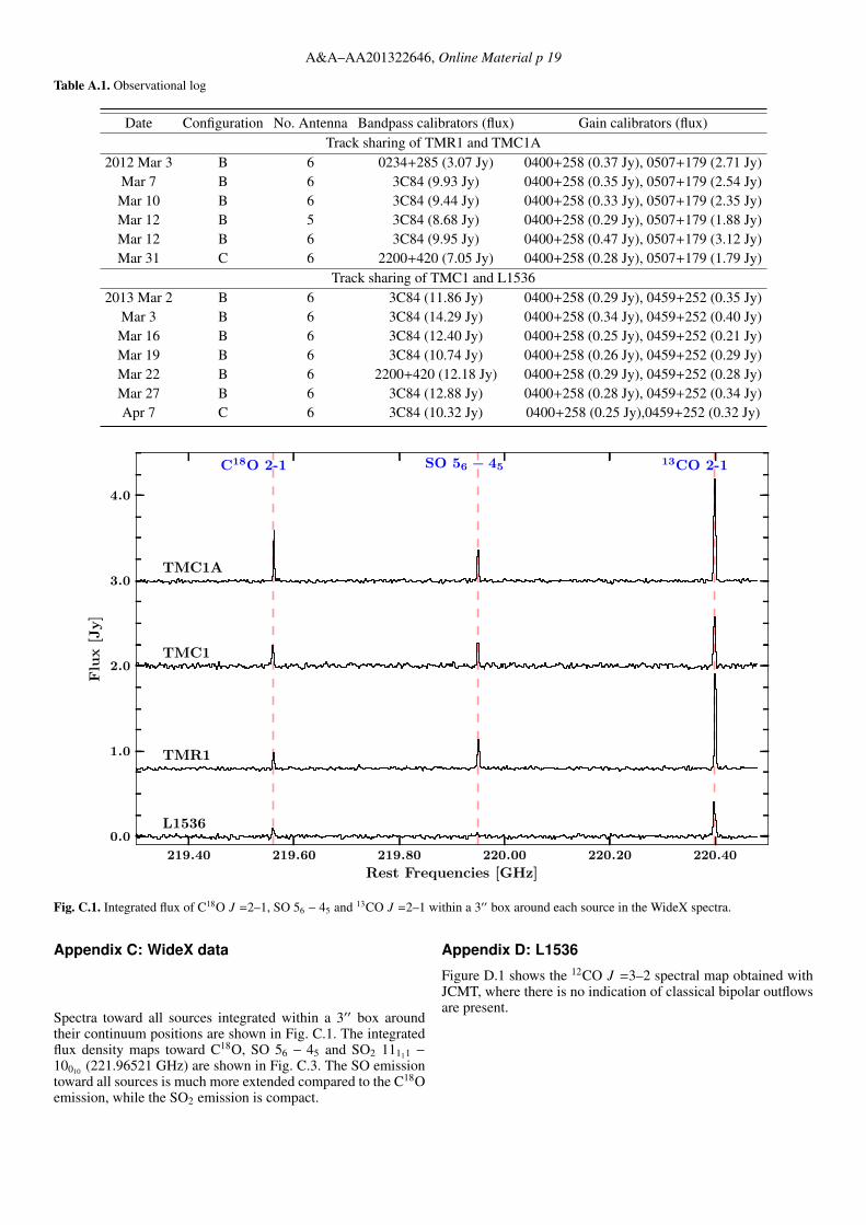
A&A–AA201322646, Online Material p 19
Table A.1. Observational log
Date Configuration No. Antenna Bandpass calibrators (flux) Gain calibrators (flux)Track sharing of TMR1 and TMC1A
2012 Mar 3 B 6 0234+285 (3.07 Jy) 0400+258 (0.37 Jy), 0507+179 (2.71 Jy)Mar 7 B 6 3C84 (9.93 Jy) 0400+258 (0.35 Jy), 0507+179 (2.54 Jy)
Mar 10 B 6 3C84 (9.44 Jy) 0400+258 (0.33 Jy), 0507+179 (2.35 Jy)Mar 12 B 5 3C84 (8.68 Jy) 0400+258 (0.29 Jy), 0507+179 (1.88 Jy)Mar 12 B 6 3C84 (9.95 Jy) 0400+258 (0.47 Jy), 0507+179 (3.12 Jy)Mar 31 C 6 2200+420 (7.05 Jy) 0400+258 (0.28 Jy), 0507+179 (1.79 Jy)
Track sharing of TMC1 and L15362013 Mar 2 B 6 3C84 (11.86 Jy) 0400+258 (0.29 Jy), 0459+252 (0.35 Jy)
Mar 3 B 6 3C84 (14.29 Jy) 0400+258 (0.34 Jy), 0459+252 (0.40 Jy)Mar 16 B 6 3C84 (12.40 Jy) 0400+258 (0.25 Jy), 0459+252 (0.21 Jy)Mar 19 B 6 3C84 (10.74 Jy) 0400+258 (0.26 Jy), 0459+252 (0.29 Jy)Mar 22 B 6 2200+420 (12.18 Jy) 0400+258 (0.29 Jy), 0459+252 (0.28 Jy)Mar 27 B 6 3C84 (12.88 Jy) 0400+258 (0.28 Jy), 0459+252 (0.34 Jy)Apr 7 C 6 3C84 (10.32 Jy) 0400+258 (0.25 Jy),0459+252 (0.32 Jy)
219.40 219.60 219.80 220.00 220.20 220.40
Rest Frequencies [GHz]
0.0
1.0
2.0
3.0
4.0
Flu
x[J
y]
C18O 2-1 13CO 2-1SO 56 − 45
TMC1A
TMC1
TMR1
L1536
Fig. C.1. Integrated flux of C18O J =2–1, SO 56 − 45 and 13CO J =2–1 within a 3′′ box around each source in the WideX spectra.
Appendix C: WideX data
Spectra toward all sources integrated within a 3′′ box aroundtheir continuum positions are shown in Fig. C.1. The integratedflux density maps toward C18O, SO 56 − 45 and SO2 11111 −
10010 (221.96521 GHz) are shown in Fig. C.3. The SO emissiontoward all sources is much more extended compared to the C18Oemission, while the SO2 emission is compact.
Appendix D: L1536
Figure D.1 shows the 12CO J =3–2 spectral map obtained withJCMT, where there is no indication of classical bipolar outflowsare present.
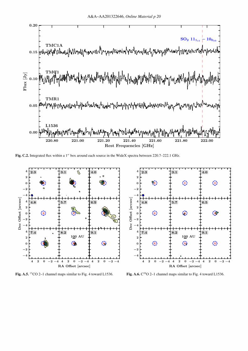
A&A–AA201322646, Online Material p 20
220.80 221.00 221.20 221.40 221.60 221.80 222.00
Rest Frequencies [GHz]
0.00
0.05
0.10
0.15
0.20F
lux
[Jy]
SO2 11111 − 10010
TMC1A
TMC1
TMR1
L1536
Fig. C.2. Integrated flux within a 1′′ box around each source in the WideX spectra between 220.7–222.1 GHz.
−4
−2
0
2
4 2.3 3.1 4.0
−4
−2
0
2
4 4.8 5.7 6.5
−4−2024
RA Offset [arcsec]
−4
−2
0
2
4
Dec
Off
set
[arcse
c]
7.4
−4−2024
8.2100 AU
−4−2024
9.1
Fig. A.5. 13CO 2–1 channel maps similar to Fig. 4 toward L1536.
−4
−2
0
2
4 2.3 3.1 4.0
−4
−2
0
2
4 4.8 5.7 6.5
−4−2024
RA Offset [arcsec]
−4
−2
0
2
4
Dec
Off
set
[arcse
c]
7.4
−4−2024
8.2100 AU
−4−2024
9.1
Fig. A.6. C18O 2–1 channel maps similar to Fig. 4 toward L1536.
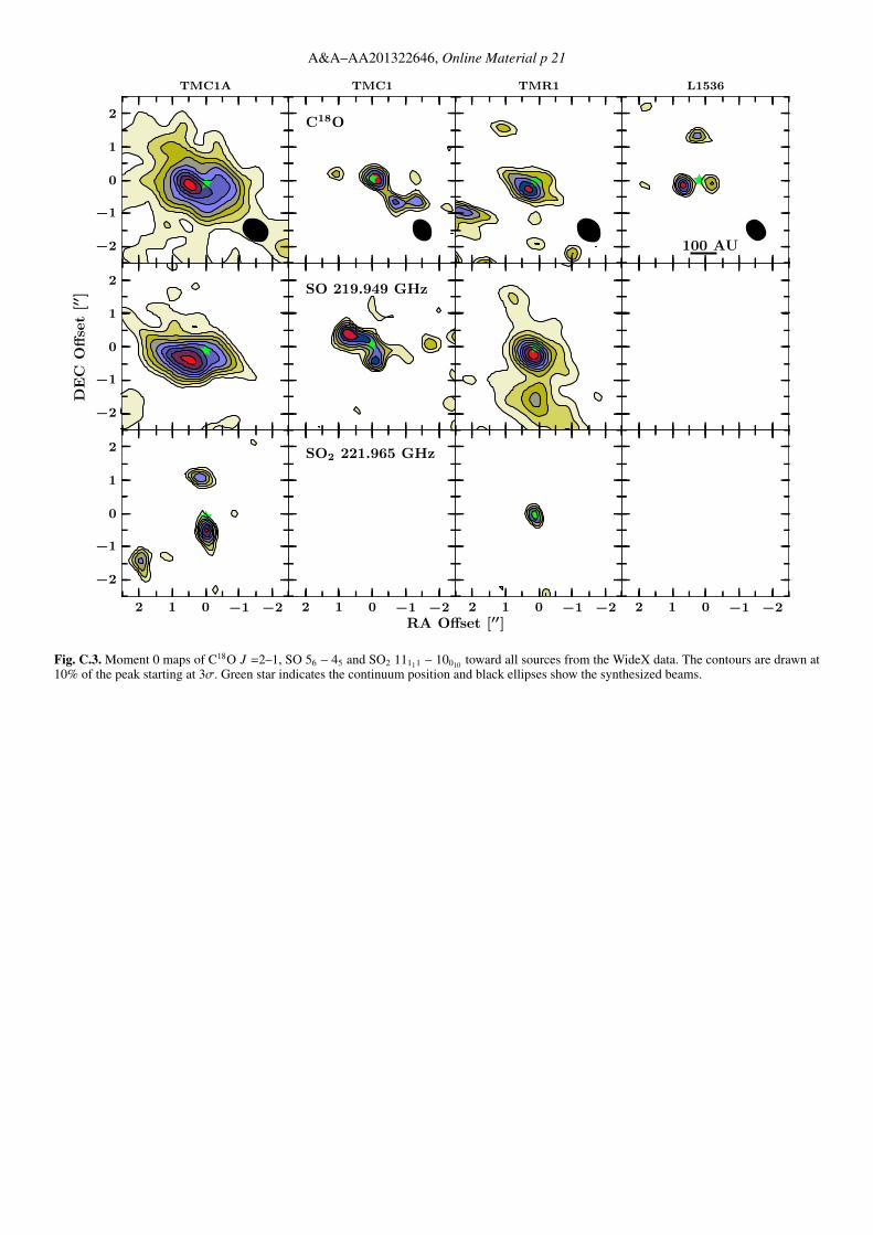
A&A–AA201322646, Online Material p 21
−2
−1
0
1
2
TMC1A
−2
−1
0
1
2
DE
CO
ffse
t[′′ ]
−2−1012
−2
−1
0
1
2
C18O
TMC1
SO 219.949 GHz
−2−1012
SO2 221.965 GHz
TMR1
−2−1012
RA Offset [′′]
100 AU
L1536
−2−1012
Fig. C.3. Moment 0 maps of C18O J =2–1, SO 56 − 45 and SO2 11111 − 10010 toward all sources from the WideX data. The contours are drawn at10% of the peak starting at 3σ. Green star indicates the continuum position and black ellipses show the synthesized beams.
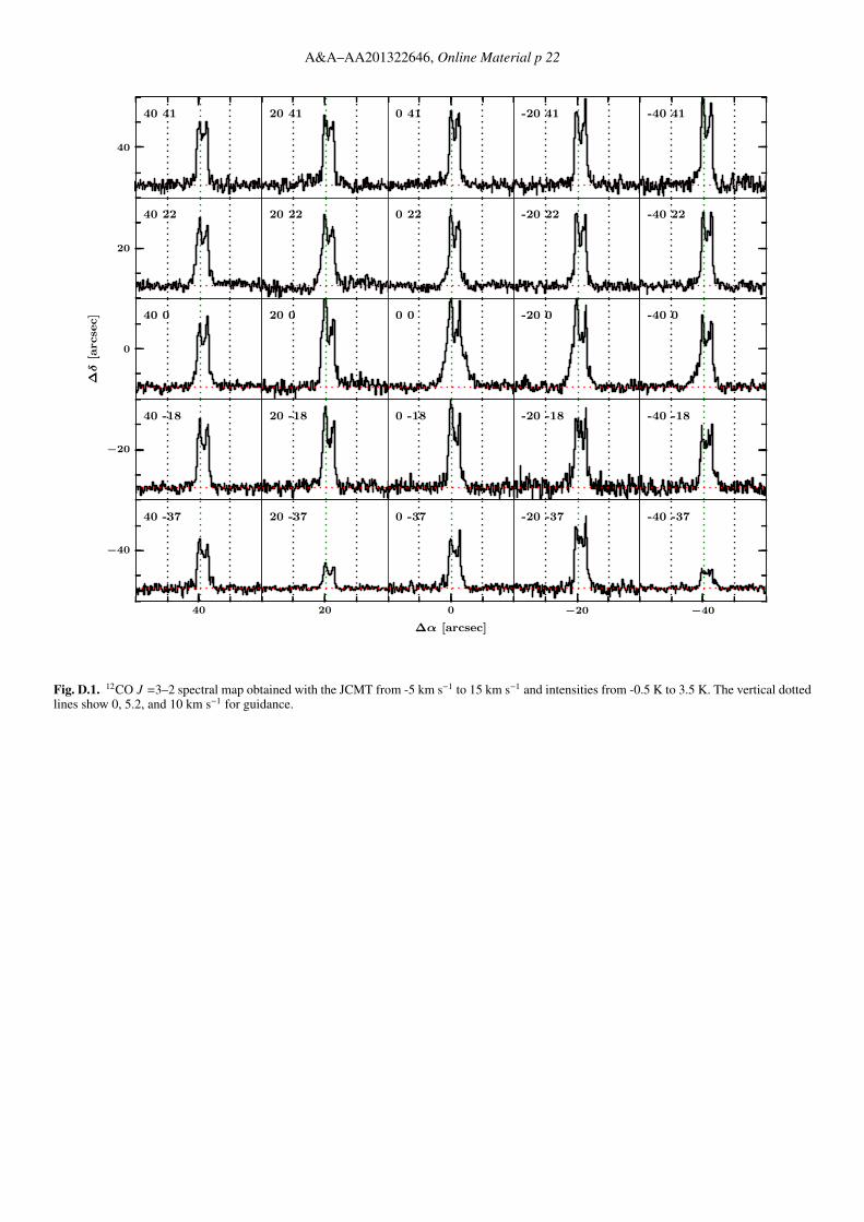
A&A–AA201322646, Online Material p 22
40 41
40 22
40 0
40 -18
40 -37
20 41
20 22
20 0
20 -18
20 -37
0 41
0 22
0 0
0 -18
0 -37
-20 41
-20 22
-20 0
-20 -18
-20 -37
-40 41
-40 22
-40 0
-40 -18
-40 -37
−40−2002040
∆α [arcsec]
−40
−20
0
20
40
∆δ
[arcse
c]
Fig. D.1. 12CO J =3–2 spectral map obtained with the JCMT from -5 km s−1 to 15 km s−1 and intensities from -0.5 K to 3.5 K. The vertical dottedlines show 0, 5.2, and 10 km s−1 for guidance.