Embed Size (px)
Citation preview

RoutePlanningAlgorithmsfor CarNavigation

CIP-DATA LIBRARY TECHNISCHEUNIVERSITEIT EINDHOVEN
Flinsenberg, Ingrid C.M.
Routeplanningalgorithmsfor carnavigation/by Ingrid C.M. Flinsenberg. -Eindhoven: TechnischeUniversiteitEindhoven,2004.Proefschrift.- ISBN 90-386-0902-7NUR 919Subjectheadings: routing / algorithms/ electronicnavigation / stochasticgraphs/combinatorialoptimisation/ graphs/ automobilism2000MathematicsSubjectClassification: 05C38,65K10,05C85
Thework describedin this thesishasbeencarriedout at theDevelopmentCenterofSiemensVDO TradingB.V. (subsidiaryof SiemensVDO Automotive) in Eindhoven,theNetherlands.It maycontainIntellectualPropertyRights(IPRs)of SiemensVDOAutomotive AG. All rightsreserved.
I.C.M. Flinsenberg 2004All rightsarereserved.Reproductionin wholeor in partis
prohibitedwithout thewrittenconsentof thecopyright owner.

RoutePlanningAlgorithmsfor CarNavigation
PROEFSCHRIFT
ter verkrijging van de graad van doctor aan deTechnischeUniversiteit Eindhoven, op gezagvande Rector Magnificus, prof.dr. R.A. van Santen,voor eencommissieaangewezendoor het Collegevoor Promotiesin het openbaarte verdedigenop
donderdag30 september2004om16.00uur
door
Ingrid ChristinaMariaFlinsenberg
geborente Helmond

Dit proefschriftis goedgekeurddoordepromotoren:
prof.dr. E.H.L. Aartsenprof.dr. J.vanLeeuwen
Copromotor:dr. J.H.Verriet
Thework in this thesishasbeencarriedoutundertheauspicesof theresearchschoolIPA (Institutefor ProgrammingresearchandAlgorithmics).IPA DissertationSeries2004-12

Preface
When I attendedthe defenseof my aunt’s thesisapproximatelynine yearsago atTilburg University, whereI just startedto studyeconometrics,the ideathat I wouldbedefendingmy own thesisonedaynever occurredto me.However, four yearsago,when professorEmile Aarts offered me a position asa PhD-studentat EindhovenUniversityof Technologyon the topic of advancedrouteplanningstrategiesfor carnavigation in cooperationwith SiemensVDO Automotive, the topic immediatelyappealedto me. NeverthelessI gave quite somethoughtto the questionwhetherIwantedto spendthe next four yearsdoing researchon this particulartopic. I havenever regrettedmy decisionto do it, andthanksto thesupportof many people,youarenow holdingtheresult.
I would especiallylike to thankmy two supervisorsprof. dr. Emile Aarts anddr. JacquesVerriet. JacquesVerriet hasbeenmy daily supervisorfor the last fouryears. I would like to thank Jacquesfor the discussionsthat usually lead to newideasand for his help on implementationissues. I would also like to thank himfor his perseverancein readingall my manuscripts. His never endingcommentsandindicationsto improve my manuscriptsreally madea difference.Furthermore,Iwould like to thankEmile Aartsfor our fruitful discussionsandfor hisconfidenceinme,whichwasvery stimulating.
Furthermore,I would like to thankEdgardenBoef, Martijn van der Horst andGraceZhu for their valuablecontributions and TeunHendriksand Karin Lim formaking suremy researchcontinuedto be useful to SiemensVDO Automotive. Iconsidermyself fortunatein having the membersof the route plannergroup fromSiemensVDO Automotive asmy colleagues.They helpedme get valuableinsightin thepeculiaritiesof routeplanningin carnavigationsystemsandwerealwaysveryhelpful in solvingproblemswith carnavigationsoftware.Furthermore,I would liketo thankmy colleaguesfrom the(Eindhoven)EmbeddedSystemsInstitute,for pro-viding a pleasantworking environmentat the university aswell. I would also liketo thankmy friendsfrom Chikara,whosefriendshipindirectly hadquitean impact.Furthermore,I amgratefulfor theinterestandsupportof my family.
Finally, I would like to thankmy parentsfor alwayssupportingme.Without theircontinuingsupportthis thesiswouldnothave beenpossible.
v

vi

Contents
1 Intr oduction 11.1 CarNavigationSystems. . . . . . . . . . . . . . . . . . . . . . . . 21.2 ProblemFormulation . . . . . . . . . . . . . . . . . . . . . . . . . 51.3 RelatedWork . . . . . . . . . . . . . . . . . . . . . . . . . . . . . 71.4 ThesisOutline . . . . . . . . . . . . . . . . . . . . . . . . . . . . . 11
2 Road Network Models 152.1 Time-IndependentPlanning. . . . . . . . . . . . . . . . . . . . . . 152.2 Time-DependentPlanning . . . . . . . . . . . . . . . . . . . . . . 182.3 StochasticTime-DependentPlanning. . . . . . . . . . . . . . . . . 202.4 TowardsaSolutionStrategy . . . . . . . . . . . . . . . . . . . . . 24
3 Partitioning 273.1 RepresentingPartitions . . . . . . . . . . . . . . . . . . . . . . . . 273.2 PartitioningObjectives . . . . . . . . . . . . . . . . . . . . . . . . 303.3 Complexity . . . . . . . . . . . . . . . . . . . . . . . . . . . . . . 363.4 Algorithmsfor Partitioning . . . . . . . . . . . . . . . . . . . . . . 403.5 Multi-Level Partitioning . . . . . . . . . . . . . . . . . . . . . . . 583.6 Conclusion . . . . . . . . . . . . . . . . . . . . . . . . . . . . . . 70
4 Time-IndependentPlanning 734.1 RepresentingRouteGraphs. . . . . . . . . . . . . . . . . . . . . . 734.2 Algorithmsfor Time-IndependentOptimumRoutePlanning . . . . 834.3 ComputationalEvaluation . . . . . . . . . . . . . . . . . . . . . . 894.4 Extensionto Multi-Level Partitions. . . . . . . . . . . . . . . . . . 994.5 Conclusion . . . . . . . . . . . . . . . . . . . . . . . . . . . . . . 101
5 Time-DependentPlanning 1035.1 Introduction . . . . . . . . . . . . . . . . . . . . . . . . . . . . . . 1035.2 Consistency . . . . . . . . . . . . . . . . . . . . . . . . . . . . . . 1065.3 Algorithmsfor Time-DependentPlanning . . . . . . . . . . . . . . 1105.4 ComputationalEvaluation . . . . . . . . . . . . . . . . . . . . . . 1115.5 Combinationwith Partitions . . . . . . . . . . . . . . . . . . . . . 1275.6 Conclusion . . . . . . . . . . . . . . . . . . . . . . . . . . . . . . 141
vii

viii Contents
6 StochasticTime-DependentPlanning 1436.1 Introduction . . . . . . . . . . . . . . . . . . . . . . . . . . . . . . 1446.2 Consistency . . . . . . . . . . . . . . . . . . . . . . . . . . . . . . 1476.3 Algorithmsfor StochasticTime-DependentPlanning . . . . . . . . 1496.4 ComputationalEvaluation . . . . . . . . . . . . . . . . . . . . . . 1526.5 Combinationwith Partitions . . . . . . . . . . . . . . . . . . . . . 1626.6 Conclusion . . . . . . . . . . . . . . . . . . . . . . . . . . . . . . 172
7 Comparisonwith Product RoutePlanners 1757.1 StandardRoutePlannerAlgorithms . . . . . . . . . . . . . . . . . 1757.2 AveragePerformanceof theC
�- andRP-Algorithm . . . . . . . . . 177
7.3 ExceptionalCasesof theRP-Algorithm . . . . . . . . . . . . . . . 1807.4 AdvantagesComparedto theRP-Algorithm . . . . . . . . . . . . . 1827.5 DisadvantagesComparedto theRP-Algorithm . . . . . . . . . . . . 1887.6 ExtendingFunctionalityof theS
�-Algorithm . . . . . . . . . . . . . 189
7.7 Conclusion . . . . . . . . . . . . . . . . . . . . . . . . . . . . . . 195
8 Conclusions 197
A Determining the AverageNumber of Edgesin a Searchgraph 201
B Moving a NodebetweenCells 203
C Partitions 207
D StochasticversusDeterministic Time-DependentRoutes 221
Bibliography 235
Notational Index 245
Author Index 251
Subject Index 255

1Introduction
Mobility is very importantin our society. Peoplelive in onecity andwork in an-other. They goto visit friendsandfamily living in differentpartsof thecountry. Evenleisuretime is not alwaysspentin their residence.DespitetheDutchgovernment’seffortsto increasetheuseof publictransportation,thecaris still themostwidely usedmeansof transportation.Everytimesomeonetravelsfrom onelocationto another(bycar),heor shefirst determinesthebestrouteto reachthedestination.Dependingonthetimeof dayandthedayof theweek,this routemaybedifferent.For example,thedriver mayknow thatacertainroadis alwayscongestedata particulartime andday.As aconsequence,hechoosesto usea differentrouteto avoid thiscongestion.
Car navigation systemsarebeingofferedasa specialfeatureof new carsof anincreasingnumberof car-brands.Thesecarnavigationsystemsarecapableof takingover someof thetasksthatareperformedby thedriver suchasreadingthemapanddeterminingthebestrouteto thedestination.They shouldalsotake daily congestionpatternsinto account.Becauseacarnavigationsystemusesabuilt-in computerto de-terminearoute,it cancomparemany differentroutesandtheuserexpectsthesystemto determinethebestpossible,or optimumroutefast. This thesisis concernedwithrouteplanningalgorithmsthatenableacarnavigationsystemto planoptimumrouteson very large real-world roadnetworks in very little time, taking daily congestionpatternsinto account.
To thatend,Section1.1briefly explainstheconceptof acarnavigationsystemaswell asthemainfunctionalityof sucha system.Therouteplanningproblemthatwe
1

2 Introduction
will try to solve is presentedin generaltermsin Section1.2. Section1.3presentsanoverview of publicationson relatedtopics.An outlineof theremainderof this thesisis presentedin Section1.4.But first, wegiveanon-comprehensive overview of acarnavigationsystem.
1.1 Car Navigation Systems
Currently, an increasingnumberof consumershasgainedinterestin car navigationequipment. Car navigation is no longer a luxury that is only for the rich. A carnavigation systemis offeredasoneof themany extrasor asanadvertisingstuntofmore andmore “middle-class”cars. In the future, car navigation equipmentmaybecomeas normal as air-conditioning. Of course,alsoother vehiclescan usecarnavigation, suchastrucks,bussesandmotorcycles. A navigation systemoffers thedriverthepossibilityto beguidedto hisdestination,by meansof spokenand/orvisualadvices. In order to achieve this, the driver first hasto enterhis destinationintothe system.Sucha destinationmay be a city center, an entirestreet,or an addressincludingahousenumber. Informationoneverypossibledestinationis containedin adatabasethatis storedonaCD or DVD thathasto beinsertedinto thecarnavigationsystem.Also datafrom externalprovidersaboutinterestingplacessuchashotelsandrestaurantsfor exampleis storedon theCD or DVD. Thedriver canaskfor a list ofall hotelsin acertainareafor example.
Figure1.1. A car navigationsystem.
Figure1.1 gives an overview of the main elementsof a car navigation system. Itshows on theleft thesensors(gyroandtacho)anda GPSsatelliteusedfor determin-ing the positionof the car. The computer, which containsthe CD or DVD player,and the screenfor displayingthe mapandvisual adviceareshown in the middle.On theright, aGSM connectionandTMC-RDSbroadcastsusedfor receiving trafficinformationareshown.
Thekey componentsof a carnavigationsystemarepositioning,i.e. determiningthe currentposition of the car on the road network, route planning, i.e. planning

1.1 CarNavigationSystems 3
a route from the position of the car to the destination,and guidance,i.e. givinginstructionsto thedriver. Schlott[1997] andZhao[1997] give anoverview of thesekey components.Figure1.2givesanoverview of themostimportantcomponentsofacarnavigationsystem.
Figure1.2. Thekey componentsof a car navigationsystem.
First, we explain positioning. In order to determinethe currentlocationof the caron the road network, a car navigation systemtries to determinethe geographicalposition of the car. This is doneby “dead reckoning” [Zhao, 1997], which is thecalculationof the geographicalpositionbasedon calibratedsensorinformation. Inparticularthedriven distancefrom the tachoandtheangularratefrom thegyro areusedto determinethe positionof the car. This positioncanbe improved by usingtheGPSpositionandspeed.Subsequently, this geographicalpositionis matchedtotheavailableroadnetwork. This is doneby computingthe likelihoodthat thecar iscurrentlyat a particularpositionon a certainroadsegment. The routepresentedtothedriver is alsousedin thismapmatchingprocess.A positiononthecurrentrouteisgivenahigherpreferencethanotherpositions.If nopositionontheroadnetwork hasasufficiently high likelihood,thecaris notpositionedonany of theroadsegmentsoftheroadnetwork, i.e. thecaris “off map”.
Oncethe positionof the car hasbeendetermined,a routecanbe plannedfromthat car position to the destination.This route is plannedusing the available roadnetwork that is storedon a CD or DVD. Thealgorithmusedfor planninga routeis(generally)basedonDijkstra’ssinglesourceshortestpathalgorithm[Dijkstra,1959].To beableto determinea routefast,severalapproximationsareused.For example,if the car positionanddestinationare locatedsufficiently far apart,only importantroadsareusedto determinethemajorpartof theroute.Furthermore,estimationsoftheremainingdistanceto thedestinationareusedto speedup theplanningprocess.
After a routehasbeenfound,thesystemprovidesthedriver with spokenand/orvisual adviceto guide him to his destination. The position of the car is usedincombinationwith thecurrentrouteto determinethenecessaryadviceandthetiming

4 Introduction
of giving advice. Usually, thedriver first receivesa warningthatheshouldprepareto makeacertainturn. Of course,thisadvicehasto begivenin time for thedriver toactuallymake thenecessarypreparations,suchaschanginglanesandslowing down.Thenthe actualadviceis given. Also this advicehasto be timed carefully. Whilethedriver is progressingtowardshis destination,thecarnavigationsystemmonitorsthe progressof the car. That is doneby comparingthe currentpositionof the carandthepresentedroute.Of course,not all drivers(correctly)follow all instructions,sometimesadriverdeviatesfrom his route.If thecaris notpositionedon thecurrentroutefor a certainamountof time, thenthesystemconcludesthedriver hasdeviatedfrom his route,anda new routeneedsto beplannedfrom thepositionof thecar tothedestination.
This thesisfocusesontherouteplanningfunctionalityof acarnavigationsystem.Carnavigationsystemsusuallyprovide theoptionto chooseamongseveraldifferentoptimizationcriteria, or cost functions. In general,the driver canchoosebetweenplanninga fastestroute,a shortestroute,a fastestroutegiving preferenceto motor-ways,anda fastestroute giving a penaltyto motorways. Also an option to avoidtoll roadsor ferriesmaybeavailable. In the future,we expectto seean increaseinthe personalizationof plannedroutes,by an increasingadaptationof the usedcostfunctionsto thepreferencesof thedriver.
Anotheraspectof real-life that influencesthe quality of a plannedroute, is thepresenceof traffic jamson the presentedroute. Traffic information, i.e. informa-tion on traffic jams, roadworks androadconditionsfor example,arereceived viaRDS-TMC(RadioDataSystem- Traffic MessageChannel),or by aconnectedGSMphone.Oneof thechallengesof anavigationsystemis to let routeplanningtake thistraffic informationinto account,andguidethedriver arounda traffic problem. Be-causeof theincreasingnumberof traffic jams,andthefrustrationof thedriver whenhegetsstuckin oneof them,thiswouldbevaluableto thedriver.
If for somereasonthedriver is notsatisfiedwith his route,heis usuallygiventheoptionto askfor analternative route. Thereasonsfor askingfor suchanalternativeroutemay vary from a reportedtraffic jam on thecurrentroute,to preferencesthatdo not correspondwith theusedcostfunction. Alternative routesaremeantto differsignificantlyfrom the presentedroute. However, if oneparticularstreetin the pre-sentedrouteis underconstruction,thedriver maynot wanta significantlydifferentroute,hejust wantsto beguidedaroundtheconstructionworks,andbackto his oldrouteagain.In mostnavigationsystemthedriver canachieve thisby askingfor a lo-cal detour. Thesystemshouldthendeterminea routethatlocally avoidstheproblemarea.

1.2 ProblemFormulation 5
1.2 Problem Formulation
A carnavigationsystemusesmapsthatcontaina roadnetwork. CDsor DVDs con-taining the roadnetwork of entireEuropearenow becomingavailable. This meansthata carnavigationsystemhasto beableto planrouteson roadnetworksthatcon-tainmillions of roadsegments.Ontheotherhand,adriverdoesnot like to wait whilehis routeis beingcalculated.Therefore,theplanningof routeshasto be doneveryfast,within a few secondstypically.
After the driver hasenteredhis destination,andthe systemhasdeterminedthepositionof thecar, a routehasto be plannedfrom thecar’s positionto thedestina-tion. Whenplanningthis route,datahasto beretrievedfrom thedatabaserepeatedly,becauseof the limited amountof internal memorythat is available to the system.Readinginformationfrom thisdatabaseis atime-consumingtask,becausetheaccessto thesecondarystorageis slow. Also thevariousprocessesinvolved in planningaroute,determiningthepositionof thecaranddisplayingthemaparecompetingforthe limited amountof computingpower. Comparedto a personalcomputer, an on-boardcarnavigationsystemhasconsiderablylesscomputingpower, dueto hardwarerestrictionsimpliedby thesystemsrequiredtolerancefor coldandheat,aswell asitsability to withstandshocks.
To measurethequalityof aplannedroute,acostfunctionis usedto make“objec-tive” comparisonsbetweenroutespossible.Of course,differentdrivershavedifferentpreferences.Determiningthecostfunction thatcorrectlyresemblesthepreferencesof a particular, or of the “average”driver, is not an easytask. Determiningsuchacostfunctionis beyondthescopeof this research,andweassumethatacostfunctionis available that correctlydescribesthe preferencesof the driver. A route that haslowestcostaccordingto the usedcost function, is calledan optimumroute. If thedriver asksfor thebestroute,thenheexpectsthat thesystemprovideshim theroutewith the absolutelylowestcost. This meansthat a car navigation systemdoesnotonly have to planaroute,but hasto plantheoptimumrouteaccordingto aparticularcostfunction.
Planningoptimumroutesfastonvery largeroadnetworksstill posesasignificantchallengeto companiesdevelopingcar navigation systems.At the sametime, tak-ing informationon daily congestionpatternsinto accountis gettingmoreimportant.Driversbecomeincreasinglydemanding,andexpect that traffic information is notonly provided,but alsousedfor determiningthebestroute.
Weaimatfindingalgorithmsandapproachesthatenableacarnavigationsystemto planoptimumrouteson very largeroadnetworks in very little time, takingtrafficinformation into account. At the sametime, it shouldremainpossibleto maintainthefull functionalityof acarnavigationsystemasdescribedin Section1.1. Also theintroductionof all kindsof new functionalityhasto bepossible.
Currentcar navigation systemsusean approximationalgorithmto plan a route

6 Introduction
faston largeroadnetworks. Ideally, wewould like to beableto planoptimumroutesfasterthancurrentsystemsplana non-optimumroute. Theroadnetworkson whichrouteshave to beplannedgenerallyconsistof millions of nodesandedges.Becauseroute planningin the car hasto be fast, it is necessary, with currenthardware, tousesomekind of pre-processing.The roadnetwork is too large to useasa wholeto searchfor anoptimumroute. Therefore,the roadnetwork hasto bedivided intosomekind of sub-networksthataresmallerandcanbesearchedmoreeffectively.
We first have to find a pre-processingalgorithmthatenablestheplanningof op-timum routes,or in otherwords,routeswith minimumcost. Usingtheresultof thispre-processingalgorithm,theplanningof optimumroutesin verylargeroadnetworkscontainingmillions of nodesshouldbefast.So,we needto find a routeplanningal-gorithmusingtheresultof thepre-processingstepthatplansoptimumroutesfast.
A challengeof a navigationsystemis to let therouteplanningtake traffic infor-mationinto account,andpossiblyguidethedriver arounda traffic problem.Currentcarnavigationsystemstake traffic informationinto accountby increasingthecostofroadsthat arecongestedwhenplanninga route. However, traffic jamsareusuallyonly reportedif they arelongerthanafew (typically two) kilometers,or if they causeasignificantdelayfor drivers.However, lessseveretraffic jamsor mild reductionsindriving speedcausedby everydaypeaktraffic arenot alwaysreported.Thesetrafficcircumstancesdo influencethe bestroutehowever. Therefore,we would also liketo take thesedaily recurringpatternsinto accountwhenplanninga route. Driversfamiliar to aparticularenvironmentalsotake thesecircumstancesinto accountwhenthey aredeterminingtheir route,andsoshoulda car navigation system.Therefore,we want to take daily congestionpatternsinto accountwhenplanninga route. Thisshouldnotonly remainpossibleby usingthepre-processingalgorithm,but theplan-ning of routesthat take thesecongestionpatternsinto accountshouldalsobe fast.Furthermore,theseroutesshouldbe thebestroutespossible,which leadsto a needfor a definitionof anoptimumroutein thepresenceof daily congestion.Finally, weneedto developa routeplanningalgorithmfor planningtheseoptimumrouteswhiletakingcongestionpatternsinto account.
Naturally, daily congestionis not exactly thesameevery day, sowe have to dealwith uncertainty. This not only requiresthe formulation of a model for handlinguncertainty, but alsothedeterminationof thequality of a routewith uncertaincost,anda routeplanningalgorithmthatdeterminesa bestpossibleroutefast.Of course,thishasto becombinedwith theuseof thepre-processingalgorithm.
Finally, thedevelopedalgorithmsmustbecompatiblewith otherfeaturesof acarnavigationsystem.For example,a new routehasto beplannedif thedriver deviatesfrom his route,or if he requestsanalternative route. Furthermore,the functionalityof a car navigation systemshouldbe (easily)extendable.The designedalgorithmsshouldnot restricttheintroductionof new featuresin thefuture.

1.3 RelatedWork 7
In determininganapproachto achieve thesegoals,we make oneimportantassump-tion. We assumethat the plannedroutesdo not influencethe congestionpatterns.If many driversown a carnavigationsystemusingthesamealgorithmto determinean optimumroute,thenall thesedriversreceive thesameadviceandtake thesameroute.This couldcausecongestionon this routewhich, in turn, mayleadto anotherroutebecomingthe optimumroute. We assumethat this is not the case,i.e., a carnavigation systemdoesnot have to take the effect of its own adviceinto account.This is not anunreasonableassumptionbecausewe believe personalizationwill be-comeincreasinglyimportantin car navigation systems.As a result, the usedcostfunctionsfor planningoptimumrouteswill differ betweendrivers. This mostlikelyleadsto differentoptimumroutesfor differentdrivers. Note that Jahn,Mohring &Schulz[2000] studytheproblemof planninggoodroutessuchthat theusageof theroadnetworkscapacityis optimized.
1.3 RelatedWork
Finding a route in a roadnetwork with minimum cost is referredto asthe shortestpathproblem.This problemhasbeenstudiedextensively in thepastdecades.Dijk-stra’s algorithm[Dijkstra, 1959] is the mostwell-known algorithmfor determiningtheshortestpathfrom onelocationto all otherlocationsin a roadnetwork. If only ashortestpathbetweentwo locationshasto bedetermined,Dijkstra’salgorithmcanbespeededupby takinganestimationof thecostfrom a locationto thedestinationintoaccount.This algorithmis calledtheA
�-algorithm[Hart, Nilsson& Raphael,1968].
If theusedestimationsatisfiesa few conditions,thentheA�-algorithmcanbeusedto
plantheshortestpathbetweentwo nodesin aroadnetwork. Also many othershortestpathalgorithmsexist, suchastheBellman-Fordalgorithm[Bellman,1958;FordJr. &Fulkerson,1962],theD’Esopo-Papealgorithm[Pape,1974]andtheFloyd-Warshallalgorithm[Floyd, 1962]. An overview is givenby Bertsekas[1998]. More recently,Thorup[1997] haspresenteda deterministiclinear time andspaceshortestpathal-gorithmfor undirectedgraphswith positive integeredgeweights.However, theA
�-
algorithm(originally in [Hart, Nilsson& Raphael,1968],seealso[Gelperin,1977]and[Pearl,1984])is themostcommonlyusedshortestpathalgorithmin geographicalnetworks.
New algorithmsfor planningtheshortestpathfrom onelocationto all otherlo-cationshave beenpresentedin [Meyer, 2001;Meyer, 2002;Meyer & Sanders,2003;Pettie,2002]. Meyer [2001] presentsalgorithmsfor planningtheshortestpathfromonelocationto all otherlocationsin arbitrarydirectedgraphswith realedgeweightsuniformly distributedin
�0 � 1� in linearaverage-casetime. Theaverage-timecomplex-
ity of computingthesepathsin parallelis studiedby Meyer[2002]. Meyer& Sanders[2003] proposeandanalyzesequentialandparallelversionsof a label-correctingal-gorithmfor thesinglesourceshortestpathproblem.Pettie[2002] presentsanalgo-

8 Introduction
rithm for determiningtheshortestpathbetweenall pairsof nodesin arbitraryreal-weighteddirectedgraphs. Wang & Kaempke [2004] presentan polynomial timealgorithm for computingthe shortestpath in distributed systems. Huang,Jing &Rundensteiner[1996] presentanalgorithmfor finding theshortestpathbetweenallpairsof nodesin a graphwhich takesthe limited amountof mainmemoryin an in-telligenttransportationsysteminto account.Chen,Daescu,Hu & Xu [2003] presentanalgorithmicparadigmfor finding thelengthof anoptimalpathwithout growing asinglesourceshortestpathtree.Findingamulti-criteriashortestpathis discussedbyGranat& Guerriero[2003]. Mandow & Perezdela Cruz[2003]discussmulti-criteriaheuristicsearchin moregeneralterms.
Very specificfor roadnetworks is thepresenceof turn restrictions.Turn restric-tionsaretraffic rulesthat forbid thedriver to make a certainmaneuver, for example,it may be forbiddento make a left turn at a particular intersection. Thesetrafficrulesor turn restrictionsform averyspecificaspectof real-life roadnetworks,thatisusuallyignoredwhendiscussingrouteplanningon real-world roadnetworks. Turnrestrictionscanbemodeledby costson adjacentroadsegments,sothatcertainturnsaregivenanadditionalcost.Turn restrictionshave beenstudiedrecentlyby Schmid[2000],Winter [2002] andSzeider[2003]. Schmid[2000] discussesforbiddenturnsor equivalently, turn restrictionswith infinite costs. He presentsseveral algorithmsandgraphreformulationsfor planningoptimumroutesif forbiddenturnsexist in aroad network. Winter [2002] considersturn costson pairs of adjacentedges. Heconstructstheline graphof theroadnetwork, andprovesthatoptimumroutesin theoriginal roadnetwork canbeplannedby applyingastandardshortestpathalgorithmto the line graph. Szeider[2003] considersthe problemof determiningwhetherasimplepathexistsbetweentwo nodesin afinite undirectedsimplegraphG with turnrestrictions(i.e. in a graphwith at mostoneedgebetweenany two nodesandwith-out loops),wherea simplepathis a routein which eachnodeappearsat mostonce.He constructsfor eachnodeu in graphG a transitiongraphthathasa nodefor eachedgeadjacentto nodeu, andanedgebetweentwo nodesif theturn betweenthetwocorrespondingedgesis allowed.He provesthattheproblemof determininga simplepathis NP-completeif thecollectionof thesetransitiongraphscontainsat leastoneoutof four setsof graphs.
For a car navigation system,a standardDijkstra-like algorithm[Dijkstra, 1959;Hart, Nilsson& Raphael,1968] is not fastenoughto plan optimumroutesin largereal-world roadnetworks.Becauseof thehighdemandsonplanningspeed,therouteplanningprocesshasto be speededup, which can be doneby pre-processingtheroadnetwork. Jung& Pramanik[2002] describea graphpartitioningapproachtospeedup theplanningprocess.They divide the roadnetwork into a numberof dis-junct subgraphsthat areconnectedby a boundarygraph. The planningprocessisspeededup, by reducingthe graphon which the optimumroute is planned. Kim,

1.3 RelatedWork 9
Yoo & Cha[1998] discusshandlingreal-timedatain combinationwith graphparti-tions.They addall edgesthatmaybesubjectto real-timedatato theboundarygraph.Henzinger, Klein, Rao& Subramanian[1997] usetheplanarseparatorsof Lipton &Tarjan[1979] to achieve a fasterrouteplanningprocess.Their theoremgiveseffi-cient theoreticboundson the runningtime of their shortestpathalgorithm,but wedo not considerthis approachto bepracticallyfeasible.Chen& Xu [2000] alsousetheseplanarseparatorsto answershortestpathqueriesin undirectedplanargraphswith non-negative edgeweights,but their appoachis basedon theembeddingof thegraphin theplane.Graphseparatorsarealsostudiedby Alber, Fernau& Niedermeier[2003]. Chan& Zhang[2001] basetheir partitioningof agraphon rectangulargridsandsubgraphsmay have nodesin common. Huang,Jing & Rundensteiner[1995]andHuang,Jing& Rundensteiner[1997]alsousesubgraphsthathavenodesin com-monbut storetheminimumpathcostbetweenevery pairof nodesin every subgraphandbetweena restrictednumberof nodepairs in the boundarygraph. Thesenodepairsareselectedaccordingto theimportanceof theedgesconnectedto thesebound-ary nodes,therebysacrificingoptimality of the plannedpaths. In [Jing, Huang&Rundensteiner, 1996;Jing,Huang& Rundensteiner, 1998] they preserve optimalityby storing all minimum pathcostsbetweenboundarynodes. Shekhar, Fetterer&Goyal [1997] studythememoryrequirementsof storingtheminimumpathcostbe-tweenevery pair of nodesfor severalnodesets,andcomparethis with thedecreasein the route planningtime resultingfrom using thesestoredminimum path costs.Fernandez-Madrigal& Gonzalez[2002] introducemultiple hierarchiesin apartitionto plana routebut their approachsacrificestheoptimality of theplannedroute.Car,Mehner& Taylor [1999]donotstoreshortestpathcostsbut useahierarchybasedonaveragetravel speedsto restrictthenumberof edgesconsideredin finding ashortestpath,therebysacrificingoptimality of the found path. Seong,Sung& Park [1998]usea similar approach.Ertl [1998] createsan implicit edgehierarchyby creatinga“radius” for every edge.Only if thedistancefrom thestartnodeor destinationnodeto theendnodeof anedgeis smallerthanits radius,theedgeis evaluatedwhenplan-ninganoptimumroutebetweenthetwo nodes.If theoptimalityof routesneedsto beguaranteed,determiningtheseradii is very time-consuming.
A roadnetwork canbepre-processedby graphpartitioning,which is studiedbyseveral authors. Berry & Goldberg [1999] comparedifferent algorithmsfor com-putinga graphpartition. Falkner, Rendl& Wolkowicz [1994] studypartitioningthenodesof a graphinto k disjoint subsetsof specifiedsizessoasto minimizethetotalweightof theedgesconnectingnodesin distinctsubsetsof thepartition.They presentanumericalstudyontheuseof eigenvalue-basedtechniquesto find upperandlower-boundsfor thisproblem,basedongraphsof severalthousandsof nodes.Huang,Jing& Rundensteiner[2000] comparealternative graphclusteringsolutionsfor storingdatain squareblocks that minimize the numberof I/O operations.They compare

10 Introduction
spatialpartitioningclustering,that exploits spatialcoordinatesandhigh locality, 2-partitioningandapproximatetopologicalclustering.Their experimentson randomlygeneratedgraphsshow that differentalgorithmsshouldbe usedfor different typesof graphs.Krishnan,Ramanathan& Steenstrup[1999] studygraphpartitioningforInternet-like structuresandrequirethatthepartitionsareconnected.Monien& Diek-mann[1997] studybisectiontechniquesfor minimizing the numberof connectionsbetweensubgraphs.Pothen[1997] studiesthe sameproblembut comparesseveraltechniques.Banos,Gil, Ortega& Montoya [2004]minimizethenumberof cutedgesallowing a pre-specifiedunbalancein thenumberof nodesin thecreatedsubgraphs.Kim & Moon [2004a] empirically study the local-optimumsolution spaceof thisproblemfor the Fiduccia-Mattheysesheuristic[Fiduccia& Matteyses,1982]. Bol-lobas& Scott[2004]giveoptimalboundsfor bipartitionsof graphswith boundedma-ximum degreeminimizing themaximumnumberof edgesin eachsubgraph.Graphpartitioningis alsostudiedby Schloegel, Karypis& Kumar[2000], Karypis& Ku-mar [1998] andKim & Moon [2004b]. Partitioning of flat terrain into polygonsisstudiedby Rowe & Alexander[2000]. Cordone& Maffioli [2004] studythe com-plexity of partitioninga graphinto a givennumberof treesgivenvariousconstraintson thelocationsandweightsof thetrees.
Anotherapproachto speedup therouteplanningprocessis by taking theavail-ablecomputationtime directly into accountwhendesigningthealgorithm.Hiraishi,Ohwada& Mizoguchi [1999] andShekhar& Hamidzadeh[1993] presentan algo-rithm that findsa sub-optimalsolutionwithin a specifiedtime. They alsostudytheprobabilitythatasolutionis foundwithin thespecifiedtime.
Planninganoptimumroutethat takesdaily congestionpatternsinto accountcanbe seenasplanninga route in a graphthat hascoststhat arenot constant. Usingtime-dependentcostscanbeseenasonemethodto modeldaily congestionpatterns.Planningfastestroutesin time-dependentgraphshasbeenstudiedby Orda& Rom[1990,1991,1996]. Wellman,Ford & Larson[1995] discusstheplanningof fastestpathswheretheedgeweightsaregivenby time-dependentprobabilitydistributions.Subramanian[1997]andChabini[2002]presentroutingalgorithmsfor thek-shortestpathproblemfor graphswith time-dependentedgecosts.Horn [2000] presentsandcomparesalgorithmsfor planninga fastesttime-dependentroute and assumesthetime-dependenttravel speedchangescontinuouslyduring the traversalof an edge.Da Cunha& Swait [2000]considertheproblemof planningaminimum-costpathina densegraphwhereeachnodecanonly be visited within a specifictime-window.Glenn[2001] discussesa similar problembut alsoallows waiting at a pre-specifiedfixed cost. Fu [2001] presentsan adaptive route planningalgorithm for handlingreal-timeinformation,andonly determinesthenext roadsegmentin theroute. Gao[2002], Gao& Chabini[2002] andChabini[2002] do thesamefor stochastictime-dependenttravel times.Azaron& Kianfar [2003]applystochasticdynamicprogram-
1.4 ThesisOutline 11
ming to find thedynamicshortestpathin stochasticdynamicnetworks,in which thearc lengthsare independentrandomvariableswith exponentialdistributions. Notethat it is not realistic to assumethat arc lengthsare exponentiallydistributed be-causethis resultsin arc lengthvariationsthatareloo large. Golshani,Cortes-Rello& Howell [1996]useDempster-Shafertheoryto representandreasonwith uncertaininformationon both costsanddistancein an unknown environmentfor routing au-tonomousvehicles. Montemanni,Gambardella& Donati [2004] andMontemanni& Gambardella[2004] usean interval of possiblevaluesto modeluncertaintyanddetermineapathwith minimummaximumdeviation from theoptimumpathcostforall possiblerealizationsof edgecosts.An overview of researchconcerningreal-timevehiclerouting problemsis presentedby Ghiani, Guerriero,Laporte& Musmanno[2003].
Updatingan optimumroutein casethe costof oneor moreedgesin the graphchanges(dueto congestionfor example),or edgesareaddedto or deletedfrom thegraphhasbeenstudiedby Frederickson[1985], Frigioni [1998], Klein & Subrama-nian [1998] andNarvaez,Siu & Tzeng[2001] for example. They have developedalgorithmsfor the dynamicmaintenanceof the minimum-costpathupona changein edgecostsor the insertionor deletionof edges.Thesealgorithmsassumetheex-istenceof a datastructure,usually the minimum-costpath tree, that is updatedincaseof a changein theavailabledatato avoid a full re-computation.Glenn[2001]discussesreoptimizationin caseof a changeddeparturetime from thestartnodeintime-dependentnetworks.
1.4 ThesisOutline
Weintroducethreeroadnetwork modelsin Chapter2. Westartwith aformaldescrip-tion of theroadnetwork andof theproblemof planninganoptimumrouteonthisroadnetwork. We ignorethepresenceof daily congestionin this model.However, in or-derto beableto take this informationinto accountwhenplanningaroute,weneedtoextendour model.Therefore,we subsequentlyintroducea time-dependentroadnet-work model.Thismodelcanbeusedto planoptimumroutesin aroadnetwork takingdaily congestioninto consideration.However, in thismodeluncertaintyin daily con-gestionis not taken into account. Therefore,we extendthe time-dependentmodelfurtherto a stochastictime-dependentroadnetwork model.This modelis suitedfortaking uncertaintyin daily congestioninto consideration.Finally, we indicatehowwe aregoing to proceed,i.e., what strategy we usein orderto endup with a routeplanningalgorithmthatenablesusto planoptimumrouteson a very large roadnet-work in very little time, takinguncertaintyin daily congestionpatternsinto accountwhenplanninga route.
As saidin Section1.2,in orderto achieve fastrouteplanning,weneedto developa pre-processingalgorithm. The resultof this pre-processingalgorithmshoulden-

12 Introduction
ableusto planoptimumroutesonvery largeroadnetworksin very little time. Chap-ter 3 describesa pre-processingapproachaswell astwo pre-processingalgorithms.We will usea partitioningapproachto pre-processthe roadnetwork. This leadstothe definition of a partitioningproblem. We show that this partitioningproblemisstronglyNP-hard.Wethenintroduceandcomparetwo approximationalgorithmsforcreatinga partition. Thepartitioningproblemcanbeextendedto createpartitionsofpartitions,whichwecall amulti-level partitionasopposedto asingle-level partition.Finally, wepresenttheconclusionson thecreationof partitions.
After we have discussedthe creationof partitionsin Chapter3, we discusstheplanningof optimumroutesin large real-world roadnetworksusingthesepartitionsin Chapter4. Daily congestionis still ignoredin Chapter4. We discussplanninganoptimumrouteusingsingle-level partitionsandpresentsomeresults.Similarly, wediscussplanningwith multi-level partitionsanddiscusstheresults.Wewill concludethat it is possibleto plan optimumrouteson very large roadnetworks in very littletime.
In Chapter5 we turn to theproblemof takingdaily congestionpatternsinto ac-countwhenplanningaroute.Wefirst discusstheplanningof optimumroutesin sucha roadnetwork. Theplanningalgorithm,thedatathatweuseto testandevaluateouralgorithm,andtheresultsarediscussed.Wealsodealwith theintegrationof thepre-processingstepandtheuseof daily congestion.As we will see,we caneffectivelyandpractically combinethe useof partitionsanddaily congestionpatternsduringrouteplanning.
Chapter6 discussesrouteplanningwith uncertaintyin daily congestion.Also forrouteplanningwith uncertainty, wefirst look attheimplicationsof takinguncertaintyinto accountfor planningoptimumroutes.Theplanningalgorithmis thendiscussed.We have alsogathereddataon uncertaintyin travel times. The resultsof the routeplanningalgorithmarepresented,andthecombinationof usingpartitionsandplan-ning with uncertaintyis discussed.Again, we will seethat usingpartitionscanbecombinedwith stochasticrouteplanningasdiscussedin Chapter6, both in theoryandin practice.
To evaluateour routeplanningalgorithms,we comparethe resultsof our routeplanningalgorithmswith theresultsof therouteplanningalgorithmusedin commer-cially availablecar navigation systemsin Chapter7. We first briefly discussrouteplanningalgorithmsas they are usedin car navigation systemsthat are currentlyon the market in order to facilitatea propercomparison.We comparethe averageperformanceof our routeplanningalgorithmwith the VDO Daytonrouteplanningalgorithmdevelopedby SiemensVDO Automotive in Eindhoven. As we will see,ouralgorithmis onaverageableto planoptimumroutesfasterthantheVDO Daytonrouteplanningalgorithmplansnon-optimumroutes. We alsodiscusssomeexcep-tional casesfrom which thebenefitsof our approachcanbeseenevenmoreclearly.

1.4 ThesisOutline 13
Subsequently, wediscusstheadvantagesanddisadvantagesof our routeplanningap-proach.Thenwe turn to theadditionalfunctionalityof a routeplanningcomponentin a carnavigationsystem.We discusswhatcanbedoneif thecostsof certainroadsegmentsin the roadnetwork change,if the driver deviatesfrom his route,or if heentersa new destination.Requestsfor analternative routeto thecurrentdestinationarealsodiscussed.As we will see,all additionalfunctionalitycanbecombinedwithourapproach.
Finally, in Chapter8, we give anoverview of themainconclusionsandachieve-ments.

14 Introduction

2RoadNetwork Models
In this chapterwe presentthreeroadnetwork models.First, we discussthemodelthat we useto plan routesin a roadnetwork if all driving timesareconstantovertime. This is the basicmodel,and it is discussedin Section2.1. We thenextendour model to incorporatetime-dependentdriving times as well as time-dependentcosts.This modelis usedto take daily traffic congestionpatternsinto accountwhenplanninga route. The time-dependentmodel is discussedin Section2.2. Finally,we extendthetime-dependentmodelsothatuncertaintyin travel timesandcostsarealsoincorporated.This stochastictime-dependentmodelis discussedin Section2.3.It canbeusedto take uncertaintyin daily congestioninto accountwhenplanningaroutein a roadnetwork.
2.1 Time-IndependentPlanning
A carnavigationsystemusesa mapcontaininga roadnetwork to planroutes.Thisroadnetwork consistsof roadsegmentsconnectedat intersections.A lot of informa-tion is storedaboutbothintersectionsaswell asroadsegments,suchascoordinates,length,speed,roadtype,numberof lanes,streetnames,housenumbers,importance,whetherit is locatedin a urbanor rural area,andso on. Furthermore,informationon illegal maneuvers,suchasa restrictionon makinga left turn at an intersection,is available. Not all availableinformationis neededto plan,for example,thefastestor shortestroutefrom onelocationto another. We now formulatea graph-theoretic
15

16 RoadNetwork Models
modelthatincorporatesthenecessaryinformationto plana route.A roadnetwork canberepresentedby a multi-graph. A multi-graphconsistsof
nodesandedges.The intersectionsin a roadnetwork form the nodesof the multi-graph. The roadsegmentsbetweenintersectionsin a roadnetwork form the edgesof themulti-graph.Becauseone-way roadsexist, all edgesaredirected.Theremayexist multiple edgesbetweentwo nodes.For example,theremayexist parallelroadswithout sidestreetsthatdiverge andjoin again.Therefore,the roadnetwork is rep-resentedasa multi-graph,whichcanhave multiple directededgesbetweenthesametwo nodes. Let N denotethe finite, non-emptysetof nodes, with �N ��� n the to-tal numberof nodes. Let E denotethe finite, non-emptysetof directededgesbe-tweenpairsof nodes.For anedgee from nodeu to nodev, we defineδ1 � e�� u andδ2 � e�� v. Our goal is to plan a routefrom onepositionto another. In a graphwechooseto representthis by planninga routefrom astartnodes to a destinationnoded. A routeis representedby asequenceof connectededges.
Definition 2.1. A route p in multi-graphG � � N � E � is a sequenceof edgesp ��e1 � � � ��� e��� , with ei � E, andδ2 � ei �� δ1 � ei � 1 � , for i � 1 � � � ������ 1. �
We sayroute p is a routefrom startnodes � δ1 � e1 � to destinationd � δ2 � e� � . De-fine E � p� as the edge set of route p, E � p����� e1 � � � ��� e��� , so E � p� containstheedgesof route p. We useN � p� to representthe nodeset of route p, so N � p���� δ1 � e1 ��� � � ��� δ1 � e� ����� � δ2 � e� ��� . Similarly, N � G� is usedto denotethe nodesetofgraphG, soN � G�!� N, andE � G� for theedgesetof graphG, soE � G�!� E. Thenum-berof edgesin a routeis denotedby L � p� , sofor p � � e1 � � � ��� e� � , we have L � p�"�#� .Furthermore,let P � G� denotethecollectionof all possibleroutesin graphG, andletP $ �&% � G� denoteall routesin graphG containing� edges.
Definition 2.2. Let e1 ande2 beedgesin graphG, andlet u andv benodesin G. Wedefineedgee2 to beadjacentto edgee1 if andonly if
�e1 � e2 � � P $ 2% � G� . Edgese1
ande2 areadjacentif andonly if eithere1 is adjacentto e2 or e2 is adjacentto e1.Furthermore,nodeu is adjacentto edgee1 andedgee1 is adjacentto nodeu if andonly if δ1 � e1 �� u or δ2 � e1 �'� u. Finally, nodeu is adjacentto nodev if andonly ifthereexistsanedgee in G with δ1 � e�� u andδ2 � e�� v or δ1 � e�� v andδ2 � e�� u.�Whenplanningaroutein aroadnetwork, thecostsof roadsegmentsandintersectionshave to be taken into account.Thesecostscanrepresentfor example,the lengthofthe roadsegment,the time neededto drive over the roadsegmentandthe costsofmakingturns.Therefore,we needto definecostfunctionsfor edges.
Definition 2.3. Thecostsof theedgesin thegraphG � � N � E � arerepresentedby afunctionwe : E �)(+* �0 wherewe � e� is thenon-negative costof edgee � E.1 �
1 ,.-0 denotesthecollectionof non-negative realnumbers.

2.1 Time-IndependentPlanning 17
Another aspectof a road network is the existenceof traffic rules. At a particularintersection,thedriver may, for example,not beallowed to make a right turn. Dueto thesetraffic rules,notall possibleroutesareallowedin a roadnetwork. Naturally,thesetraffic ruleshave to be incorporatedinto our model (otherwiseillegal routesmaybepresentedto thedriver). Traffic rulescanbemodeledby a costfunctiononpairsof adjacentedges.If a traffic rule exists that forbids thedriver to go from oneroadsegmentto another, thenaninfinite costis associatedwith thatpair of adjacentedges.
Definition 2.4. Definewr : P $ 2% � G��)(/* �0 �0� ∞ � . If wr � � e1 � e2 � ��1 0, thenwe saythereexistsa rule from edgee1 to e2 with rule costwr � � e1 � e2 � � . �In theremainderof this thesiswe denotewr � � e1 � e2 � � by wr � e1 � e2 � . A roadnetworkcanbe representedby a multi-graphthat hasall theseproperties.This leadsto thefollowing definitionof a roadgraph.
Definition 2.5. A roadgraph is a tupleG � � N � E � we � wr � . �Two differentoperationson (road)graphsaredefinedin Definition2.6.
Definition 2.6. Theunionof two graphsG1 � � N1 � E1 � andG2 � � N2 � E2 � is definedasG1 � G2 � � N1 � N2 � E1 � E2 � . Wedefinethedifferenceof graphG1 with graphG2
asG1 2 G2 � � N � E1 2 E2 �3� � N1 2 N2 ��� E1 2 E2 � . �Now, we candefinethecostof a route. Thetotal costof a routeis equalto thesumof thecostsof all edgesin theroute,plusthecostsof all ruleson theroute.
Definition 2.7. Theroutecostof a routeis representedby wp : P � G�"�.(+* �0 �4� ∞ � .Let p � � e1 � � � ��� e��� � P � G� . Wedefine
wp � p�5� ∑e6 E $ p% we � e�87 �:9 1
∑i ; 1
wr � ei � ei � 1 � . �We denotethe costof an optimumroutefrom startnodes to destinationnoded inroadgraphG by w
�p � G � s� d � .
Whenoneis planninga route in a roadgraph,it hasto be checked whethertheroutedoesnot containany forbiddenturns. Thereforewe definea feasibleroute. Afeasiblerouteis a routethatdoesnotcontainany forbiddenturns.Notethatone-waystreetsarenot formulatedastraffic rulesandcanonly becontainedin a routein thealloweddirection,asfollows from Definition 2.1. Therefore,infeasibility cannotbecausedby one-way streets.
Definition 2.8. A feasibleroutep is a routethatsatisfieswp � p�=<� ∞. �In a carnavigationsystem,a routehasto beplannedfrom thecar to thedestinationthatis specifiedby thedriver. Weconsiderthefollowing problem.

18 RoadNetwork Models
Problem 2.1. Plana route p in roadgraphG, from a nodes to a noded, suchthatwp � p� is minimum. �2.2 Time-DependentPlanning
In Section2.1weintroducedthetime-independentmodel.Costsin thismodeldonotdependonthetimeof day. However, certainpropertiesof aroadnetwork changeovertime. Roadsmaybeclosedduringspecifictime periods.For example,a roadcanbeclosedfor constructionwork duringseveralhoursor days.Furthermore,duringrushhoursthedriving timeof arouteis typically longer. In orderto take this into account,we extendour time-independentmodel, so that it canalso handletime-dependentcosts.In thissectionwe introducethetime-dependentmodel.
We assumethat the nodeandedgesetsof a roadgraphareconstantover time,and that only the costschangeover time. This posesno restrictionbecauseif anedgeis not availableat certaintime intervals, this canbe modeledfor examplebysettingtheedgecostequalto infinity during thosetime intervals. So,we introducetime-dependentedgeandrulecosts.Weassumethattime t � * �0 .
Definition 2.9. Wedefinethetime-dependentedge costfunctionaswte : E >?* �0 �@(* �0 �0� ∞ � . wt
e � e� t � is thecostof edgee � E if thedriver departsfrom δ1 � e� at timet � * �0 . The time-dependentrule cost function is definedaswt
r : P $ 2% � G�">A* �0 �@(* �0 �B� ∞ � . wtr � � e1 � e2 ��� t � is thecostof a ruleon adjacentedgepair
�e1 � e2 � � P $ 2% � G�
for adriver departingfrom nodeδ2 � e1 �C� δ1 � e2 � at time t � * �0 . �In theremainderof this thesiswedenotewt
r � � e1 � e2 ��� t � by wtr � e1 � e2 � t � . Having intro-
ducedtime-dependentcosts,wealsoneedto determinethetimeof traversinganedge,or makinga turn. Thedriving time of anedgeis givenby a driving time functiont t
e,andtheturningtimeof a turn is givenby functiont t
r.
Definition 2.10. Thedriving timefunctionis afunctiont te : E >D* �0 (E* �0 �?� ∞ � , that
givesfor everyedgethetimeit takesto traversethatedge,startingthetraversalof theedgeat time t. Theturningtimefunctionis afunctiont t
r : P $ 2% � G�)>F* �0 (G* �0 �A� ∞ � ,thatgivesfor every rule thetime it takesto make thecorrespondingturn,startingthetraversalof thesecondedgeat time t. �The driving time neededto traverseedgee startingat time t is denotedby t t
e � e� t � .The turning time at time t of a rule on a pair of adjacentedgese1, e2 is given byt tr � � e1 � e2 ��� t � which we denoteby t t
r � e1 � e2 � t � . By allowing a positive turningtime, itis possibleto take waiting timesfor traffic lights into account. If the timing of thetraffic lights is known thenwecantake into accountthetimethedriverhasto wait forthenext greenlight. Notethatbecausethetiming of traffic lightscanbedifferentfortraffic that is going in differentdirections,we cannotspreadthis time over differentedges. If a driver hasto wait for a ferry for example,the additionalcostscanbeincorporatedinto theedgefunctionsof thegraph.

2.2 Time-DependentPlanning 19
This leadsto thefollowing definitionof a time-dependentroadgraph.
Definition 2.11. A time-dependentroadgraphGt is a tupleGt � � N � E � wte � wt
r � t te � t t
r � .�To make it possibleto determineroutesin atime-dependentroadgraph,it is alsonec-essaryto extendourdefinitionof arouteto incorporatetime. Therefore,weformulatea time-route.
Definition 2.12. Givena time-dependentroadgraphGt � � N � E � wte � wt
r � t te � t t
r � , a time-routeis givenby a tupleπ � � p � t � . Herep � � e1 � � � ��� e� � is a routein Gt andt � * �0is thedeparturetime from δ1 � e1 � . �Now we candeterminethearrival time of thedriver at thedestination.Giventime-routeπ � � � e1 � � � ��� e� ��� t1 � , thearrival timeat thedestinationis t � � 1, given that t1 isthe departure time of the driver from the start node,t2 � t1 7 t t
e � e1 � t1 � and ti � 1 �ti 7 t t
r � ei 9 1 � ei � ti �H7 t te � ei � ti 7 t t
r � ei 9 1 � ei � ti � � for i � 2 � � � ����� . This leadsto thefollowingdefinitionof thetotal routecostof a time-route.
Definition 2.13. Givenatime-dependentroadgraphGt anddeparturetime t1, let π �� p � t1 � be a time-routein Gt with p � � e1 � � � ��� e� � anddeparturetime t1 � * �0 . Thetotal routecostsof time-routeπ aregivenby
wp � π �5� wte � e1 � t1 �87 �∑
i ; 2
wte � ei � ti 7 t t
r � ei 9 1 � ei � ti � �87 �∑i ; 2
wtr � ei 9 1 � ei � ti ���
with t2 � t1 7 t te � e1 � t1 � andti � 1 � ti 7 t t
r � ei 9 1 � ei � ti �I7 t te � ei � ti 7 t t
r � ei 9 1 � ei � ti � � for i �2 � � � ����� . �We denotethe costof an optimum, i.e. minimum-costroute from start nodes todestinationnoded in a time-dependentroadgraphGt by w
�p � Gt � s� d � .
For anedgethatcannotbetraversedor a turn thatcannotbemadeduringa par-ticulargiventime interval, we have to determinetheedgeandrulecostandduration.If waiting is notallowedfor aparticularedgeor rule,thenwesettheedgeor rulecostanddurationduring therestrictedtime interval equalto ∞. Consequently, all routesthat starttraversingthatedgeor makingthat turn during the restrictedtime intervalhave a routecostandtime equalto ∞, andareinfeasible. If waiting is allowed fora particularedgeor rule, thenthedurationof traversingtheedgeor makingtheturnduringarestrictedtime interval is setequalto thetime from themomentof arrival tothemomenttheedgeor rule is allowedagain(i.e. thewaiting time),plusthedrivingtime of the edgeor turning time of the rule at that time. The costof the edgeorrule (during the restrictedtime interval) is setequalto the costof waiting from themomentof arrival to themomenttheedgecanbetraversedor the turn canbemadeagain,plus thecostof theedgeor rule at that time. Note that if anedgecanbetra-versedor a turncanbemadeatall times,thenpostponingthetraversalof theedgeor

20 RoadNetwork Models
makingof theturn is not allowed(i.e. waiting is not allowedfor theseedges).Onlyfor anedgethatcannotbetraversedor a turn thatcannotbemadeduringaparticulargiventimeinterval, waitingmaybeallowed(dependingontheselectededgeandrulecostandtime functions),but thetime of departureandresultingcostaredeterminedbeforehandandincorporatedin theedgeandrule timeandcostfunctions.
Now that we have defineda time-routein the time-dependentroadgraph,it isnecessaryto definewhena time-routeis feasible.Becausethetotal routecoststakethearrival time at a nodeinto account,it is sufficient to checkif the routecostsarefinite.
Definition 2.14. Let Gt be a time-dependentroadgraph,and π a time-routein Gt.Time-routeπ is feasibleif andonly if wp � π �J ∞. �Ourproblemcannow beformulatedasfollows.
Problem 2.2. Plana time-routeπ in Gt from a startnodes to a destinationnodedsuchthatwp � π � is minimum. �2.3 StochasticTime-DependentPlanning
The time-dependentcostsfrom Section2.2 canbe usedto modelstructuraldelaysin travel time thatarefor examplecausedby heavy traffic duringrushhours.In thiswayit becomespossibleto taketheeffectof congestioninto accountwhenplanningaroute,evenbeforeatraffic jamreporthasbeenissued.Furthermore,smallreductionsin travel speedcanbe taken into account,while a traffic jam is only reportedwhenthe travel time hasdrasticallyincreased.However, theusedtravel speedscannotbeassumedto beequalto the travel speedthedriver really experiencesat themomenthestartstraversingaparticularroadsegment.Therefore,in thissectionwe introduceuncertaintyinto ourmodel.
Thefunctiont te � e� t � denotesthetimeit takesfor adriverto traverseedgeestarting
at time t. In caseof a traffic jam, or a reducedtravel speed,bothwte � e� t � andt t
e � e� t �arestochastic,becausetheexact travel speedandthereforeboththecostof theedgeandthedriving time of thatedgeareunknown. Usually, thecostof anedgedependson the driving time. Of course,the varianceof the edgecostcanalwaysbe set to0, if no uncertaintyexists. Also without traffic jamstravel timesareuncertain,forexampledueto traffic lights,which canbemodeledby turningtimesandrule costs.However, we assumethat neitherthe costsnor the durationof rulesaresubjecttouncertainty.
Wefirst definethestochasticedge cost, andthestochasticdriving time.
Definition 2.15. Therandom(stochastic)variablewte � e� t � on domain * �0 �4� ∞ � de-
notesthestochastic(time-dependent)edge costof edgee for departuretime t � * �0 .Therandom(stochastic)variablet t
e � e� t � on domain* �0 �4� ∞ � denotesthestochastic(time-dependent)driving timeof edgee for departuretime t � * �0 . �

2.3 StochasticTime-DependentPlanning 21
This leadsto thedefinitionof astochasticroadgraphGt.
Definition 2.16. We definea stochastic(time-dependent)roadgraphasa tupleGt �� N � E � wte � wt
r � t te � t t
r � . �The introductionof stochastictravel timescausestheneedfor a new definitionof astochastictime-route, becausethedeparturetimefor eachedgein arouteis nolongeragivenconstantbut astochasticvariable.
Definition 2.17. Givenastochastictime-dependentroadgraphGt, astochastictime-routeπ is definedasπ � � p � t �"� � � e1 � � � ��� e� ��� t � , with p a routein graph � N � E � andt � * �0 thedeparturetime from δ1 � e1 � . �In Definition 2.19, we definethe cost of a stochasticroute. But first we needtointroducesomeadditionalnotation.
Definition 2.18. Let x beastochasticvariable.Themeanof x is denotedby µ � x � andthevarianceby σ2 � x� . Thecoefficientof variation of x, c � x� , is equalto σ $ x %
µ $ x% , whereσ � x� denotesthestandard deviation of x. �Definition 2.19. Given a roadgraphGt anda stochastictime-routeπ � � p � t1 � withp � � e1 � � � ��� e��� , thestochasticcostof π is definedas
wp � π �5� wte � e1 � t1 �87 �∑
i ; 2
wte � ei � ti 7 t t
r � ei 9 1 � ei � ti � �87 �∑i ; 2
wtr � ei 9 1 � ei � ti ���
with t2 � t1 7 t te � e1 � t1 � , and ti � 1 � ti 7 t t
r � ei 9 1 � ei � ti �87 t te � ei � ti 7 t t
r � ei 9 1 � ei � ti � � for i �2 � � � ����� . �The stochasticcostof stochasticroute π is very difficult to determinebecausethedriving times are stochasticand the edgeand rule costsdependon the stochasticdeparturetime from the startnodeof an edge. Checkingthe feasibility of a routecannotbedonesoeasilyanymore. Specifically, thearrival time at thedestinationisuncertain,so it is possiblethat the routehasan infinite costwith a certainpositiveprobabilitystrictly lowerthan1. Thismeansthatit is possiblethatarouteturnsouttobefeasibleor infeasible,eachwith apositiveprobability. However, theconditionthatwp � π �KJ ∞ canbegeneralizedin a relatively straightforward mannerto Pr � wp � π �J∞ ��L ε, which meansthat the probability that the routehasa finite costhasto begreaterthanor equalto ε. If ε � 1 thenit is known that theroutealwayshasa finitecost.
Definition 2.20. Let Gt be a stochastictime-dependentroadgraph,and π � � p � t � astochastictime-routein Gt. Time-routeπ is ε-feasibleif andonly if Pr � wp � π �5J ∞ �5Lε, with ε � � 0 � 1� . �

22 RoadNetwork Models
If a route is not 1-feasiblethereis a strictly positive probability that the routehasinfinite costs,sotheexpectedroutecostis infinite. Becauseof thecomplicateddeter-minationof thestochasticroutecost,wealsodefinetheestimatedcostof astochasticroute.For a routethatis not1-feasibletheexpectedestimatedroutecostmaystill befinite. Note thatwe assumethat thecostof an edgein a routeonly dependson thedeparturetime, andnot (directly) on thecostof theprecedingedgein the route,sothecostsandtravel timesof adjacentedgesareassumedto beindependent.
Definition 2.21. Givena roadgraphGt, a stochastictime-routeπ � � p � t1 � with p ��e1 � � � ��� e��� , andβ � γ � * �0 , the estimatedcostof stochasticroute π for given β � γ is
definedaswp � π �5� µ � wp � π � �87 β M σ � wp � π � � , with
µ � wp � π � �N� µ � wte � e1 � t1 � �87 �
∑i ; 2
µ � wte � ei � ti 7 t t
r � ei 9 1 � ei � ti � � �87 �∑i ; 2
wtr � ei 9 1 � ei � ti ���
σ2 � wp � π � �N� σ2 � wte � e1 � t1 � �37 �∑
i ; 2
σ2 � wte � ei � ti 7 t t
r � ei 9 1 � ei � ti � � ���with
t2 � t1 7 µ � t te � e1 � t1 � �37 γ M σ � t t
e � e1 � t1 � ���ti � 1 � ti 7 t t
r � ei 9 1 � ei � ti �87 µ � t te � ei � ti 7 t t
r � ei 9 1 � ei � ti � � �7 γ M σ � t te � ei � ti 7 t t
r � ei 9 1 � ei � ti � � ��� for i � 2 � � � ����� . �The factorβ is usedto includethe standarddeviation of the routecostin the routecost.If β is largethenthedriver hasa lot of aversionagainstuncertainty, andtheop-timum routecostwill generallyhave a lower standarddeviation, but a highermean.The factorγ is usedto increasethe travel time peredge.If γ is large thentheprob-ability that thedriver arrivesearlierthanestimatedis high. We assumeβ andγ arefixed,but arbitrary.
In orderto determinewhich routeis theoptimumstochasticroute,we first needto be ableto orderstochasticroutesaccordingto their quality. Let x and y be tworandomvariables. If x O y thenwe say x is asleastasgoodas y. We assumethatrelation“ O ” is apartial order on asetS, see[Brightwell & West,2000].
Definition 2.22. A relation“ O ” is a partial order on asetS, OFP S > S, if it has
Reflexivity: a O a for all a � S;Antisymmetry: a O b andb O a impliesa � b;Transitivity: a O b andb O c impliesa O c � �
If any two variablescanbecomparedby relation“ O ” then“ O ” is a total order on asetS, see[Brightwell & West,2000].

2.3 StochasticTime-DependentPlanning 23
Definition 2.23. A relation“ O ” is a total order on asetS, OFP S > S, if it has
Reflexivity: a O a for all a � S;Antisymmetry: a O b andb O a impliesa � b;Transitivity: a O b andb O c impliesa O c;Comparability: for any a � b � S, eithera O b or b O a � �
If a O b andb <O a thenwe denotethis by a Q b. For a given relationfor a setofstochasticroutecosts,we defineanoptimumstochasticrouteasfollows.
Definition 2.24. Let “ O ” be a partial orderon the stochasticroutecostswp � π � . Astochasticroute π1 � � p1 � t � with stochasticcost wp � π1 � is an optimumstochasticrouteif andonly if theredoesnotexist astochasticrouteπ2 � � p2 � t � with stochasticcostwp � π2 � suchthatwp � π2 �'Q wp � π1 � . �If wedecideto usethestochasticroutecostto measurethequalityof aroute,thenweneedto basetherelationof thestochasticroutesonthisstochasticroutecost.Becausethe averageroutecostand its standarddeviation are the most importantfactorsindeterminingwhich route is preferred,we usethe following relation for stochasticroutecosts.Notethat this relationis a total ordering.Let wp � π1 � andwp � π2 � denotethestochasticcostor travel timeof two routesfor givenβ � γ � * �0 .
If µ � wp � π1 � �87 βσ � wp � π1 � �"J µ � wp � π2 � �37 βσ � wp � π2 � � thenwp � π1 �"Q wp � π2 � .If µ � wp � π1 � �87 βσ � wp � π1 � �"R µ � wp � π2 � �37 βσ � wp � π2 � � thenwp � π1 �"O wp � π2 � .If µ � wp � π1 � �87 βσ � wp � π1 � �C� µ � wp � π2 � �37 βσ � wp � π2 � � thenwp � π1 �C� wp � π2 � .
Notethatthiscorrespondsto usingtheestimatedcostof astochasticrouteto measurethequality of stochasticroutes.We denotethecostof theoptimumroute(accordingto the estimatedroutecost) from startnodes to destinationnoded in a stochastictime-dependentroadgraphGt by w
�p � Gt � s� d � .
We canchooseto let thequality of a stochasticroutebedirectly determinedbythestochasticcostof the route. We canalsochooseto minimize theestimatedcostof a route.This leadsto thefollowing two routeplanningproblems.
Problem 2.3. Plana stochastictime-routeπ in Gt, from a nodes to a noded, suchthateitherwp � π � is optimumaccordingto anordering“ O ” or suchthatµ � wp � π � �S7βσ � wp � π � � is minimum. �Minimizing µ � wp � π � �S7 βσ � wp � π � � canbeusedto let thedriver indicatethe impor-tanceof takinguncertaintyinto accountwhenplanningaroute.Forexamplefor β � 1a decreaseof 10 minutesin theexpectedtravel time anda decreaseof 10 minutesinthestandarddeviationof thetravel timeareconsideredequallyimportant.For highervaluesof β reducinguncertaintybecomesmoreimportantthanreducingtheexpectedtravel time. For lower valuesof β thesituationis exactly theotherwayaround.

24 RoadNetwork Models
2.4 Towards a Solution Strategy
A very importantaspectof planninga routein a carnavigationsystemis thetime ittakesfrom themomentthedriver requestsguidanceuntil hereceiveshis first advice.We call this the time to first advice. The time to first adviceshouldbe assmall aspossible,becausea driver doesnot like to wait while the systemis computinghisroute.Oncehereceivesadvice,thesystemcancontinueplanning,but this time is ingeneralnotexperiencedaswaiting time. Anotherimportantaspectof routeplanningin carnavigationsystemsis thequality of theplannedroute.As saidin Sections2.1,2.2 and2.3, we aim at planningrouteswith minimum cost,or in otherwords,op-timum routes.However, thenumberof edgesin roadgraphsusedby car navigationsystemsis very large. The standardA
�-algorithm[Hart, Nilsson& Raphael,1968]
is anefficient algorithmfor planningroutesfrom a singlestartnodeto a singledes-tination node. In fact, theredoesnot exist an algorithmfor planningsinglesource,singledestinationroutesin generalgraphsthatis moreefficient in worst-case,aswasshown by Gelperin[1977]. However, usingthestandardA
�-algorithm(or Thorup’s
algorithm[Thorup,1997])to plananoptimumroutein a largereal-world roadgraph,is not fastenoughfor routeplanningin carnavigationsystems.
Our first objective is to plan optimumroutesin large roadgraphsconsiderablyfasterthanthestandardA
�-algorithm. In orderto increasethe routeplanningspeed
andmaintainthepossibilityto planoptimumroutes,wechooseto usepre-processing.By pre-processingthe roadgraph,we performsomework on planningan optimumroutebeforehand.By usingthe resultsof the pre-processingstepduring the actualrouteplanning,thespeedof the routeplanningalgorithmcanbe increaseddramati-cally. In thepre-processingstep,wepartitiontheroadgraphinto anumberof disjointsubgraphs,called cells. The resultingdivision of the roadgraphis called a parti-tion. The pre-processingstepis describedin detail in Chapter3. In orderto studytheeffect of thepre-processingstep,we studytheplanningof optimumroutesin atime-independentroadgraphG in Chapter4. We particularly focuson the numberof iterationsneededby the route planningalgorithmto plan optimumroutes. So,Chapter4 focusseson the routeplanningspeed.Becausepre-processingis usedtoincreasetheplanningspeed,we alsostudythequality of thecreatedpartitions.
After achieving our first objective in Chapter4, we turn to planningoptimumroutesin time-dependentroadgraphsin Chapter5. We first discussplanningop-timum time-dependentroutesin a time-dependentroadgraph. For someof thesetime-dependentroadgraphs,it is optimal to delay the arrival at a nodeto achieveanoptimumtime-dependentroute.Naturally, this greatlycomplicatesthesearchforan optimal route. Thereforewe introducethe conceptof consistency. If the road-graphis consistent,thenwecanuseamodifiedstandardshortestpathalgorithmsuchastheA
�-algorithmto planoptimumroutes.If theroadgraphis not consistent,using
suchanalgorithmmayresultin non-optimumroutes.We thendiscusstheeffectsof

2.4 TowardsaSolutionStrategy 25
planningfastestroutesin time-dependentroadgraphsby planningroutesthroughtheNetherlandsusingrealisticdriving speedsthat leadto a consistentroadgraph.Sec-ondly, wediscusstheintegrationof planningtime-dependentroutesusingapartition.We will seethatrouteplanningin time-dependentroadgraphscanbecombinedwithusingthepartitionsintroducedin Chapter3. As a resultalsotime-dependentroutescanbeplannedfast.
Finally, we studytheplanningof stochastictime-dependentroutesin Chapter6.Also for stochasticplanning,consistency of theusedroadgraphsis animportantissueto assesstheoptimality of the plannedroutes.Becauseof the complexity of deter-mining thestochasticcostof a routeandthelimited planningtime availableto a carnavigation system,we plan stochasticrouteswith a minimum estimatedstochasticcost. In particular, we plan fasteststochasticroutesthroughthe Netherlandsto in-vestigatethe usefulnessand behavior of stochastictime-dependentplanning. Theintegrationof usingpartitionswith stochastictime-dependentplanningis alsodis-cussed.Wewill seethatalsotheplanningof stochastictime-dependentroutescanbecombinedwith theuseof partitions.

26 RoadNetwork Models

3Partitioning
As wasexplainedin Section2.4,planninganoptimumrouteon a real-world roadnetwork containingmillions of nodesandedges,takestoo long if astandardshortestpathalgorithm,suchasDijkstra’s algorithm[Dijkstra, 1959]is used.Thenumberofedgesthat have to be examinedin orderto plan an optimumrouteis just too large.In thischapter, wediscussanapproachthatenablesusto reducethesizeof theroad-graphusedfor planningroutes,while it remainspossibleto plananoptimumroutebetweenany two nodesin the road network. This approachis basedon the con-structionof a so-calledpartition. We definea partition in Section3.1. Section3.2discussesthecriteriausedfor determiningthequality of a partition. Thecomplexityof determininga partition with maximumquality is discussedin Section3.3. Wewill seethat this problemis stronglyNP-hard. Sinceit is generallybelieved that itis not possibleto determinean optimumsolutionefficiently for NP-hardproblems,wediscusstwo approximationalgorithmsfor creatingapartitionin Section3.4.Sec-tion 3.5discussesa possibleextensionto multi-level partitions.Theconclusionsarepresentedin Section3.6.
3.1 RepresentingPartitions
The input of a route planningalgorithm, beforeany pre-processing,consistsof aroadgraph,for examplethe roadgraphin Figure3.1. This roadgraphcanbedividedinto severalsubgraphs,eachconsistingof a setof nodesanda setof edges.Sucha
27

28 Partitioning
subgraphis calleda cell. Every nodein a roadgraphis containedin exactly onecell.All edgesof the original graphthat connectnodesof a singlecell arealsopart ofthatcell andarecalledinternal edges. Cellsusuallyareformedby highly connectedsubgraphsof the original roadnetwork. For example,a city suchasEindhoven orAmsterdammay form a cell. For a roadnetwork of a city, cells maybe formedbydistrictssuchastheBijlmer in Amsterdam.Figure3.2givesthecellsof theroadgraphin Figure 3.1 after the roadgraphhasbeendivided into four cells, representedbyroundedsquares.
Thereareedgesthatconnectnodesfrom differentcells. Suchanedgeis calledaboundaryedge. The two endnodesof a boundaryedgearecalledboundarynodes.All other nodesare called internal nodes. This leadsto a collection of boundarynodesandboundaryedges,the boundarygraph, that is not necessarilyconnected.Figure3.3givestheresultingboundarygraphfor thispartition.
Definition 3.1givestheformaldefinitionof apartitionof a roadgraphG.
Definition 3.1. Let G � � N � E � we � wr � bea roadgraph,thena partition of G is a setof roadgraphs� C1 � � � ��� Ck � whereCi � � Ni � Ei � we � wr � is a roadgraphinducedby thenodesetNi, suchthatNi T Nj � /0, for every i <� j, and � k
i ; 1Ni � N. Furthermore,forall rulesin G, suchthatwr � e1 � e2 �51 0, therehasto exist aCi � � C1 � � � ��� Ck � suchthate1 � e2 � Ci. Theedgeandrule costsof cell Ci areequalto theedgeandrule costsofthecorrespondingedgesandrulesin G. �Definition 3.1 definesthe cells of a partition,andits costs. Thesecells areusuallyconnectedby boundaryedges.Definition3.2givestheformaldefinitionof boundaryedges.
Definition 3.2. Given a partition � C1 � � � ��� Ck � of roadgraphG � � N � E � we � wr � , thesetof boundaryedgesis givenby EB � E 2 �U� k
i ; 1E � Ci ��� . �Thenodesthatareconnectedby theseboundaryedgesarecalledboundarynodesandaredefinedin Definition3.3.
Definition 3.3. Given a partition � C1 � � � ��� Ck � of roadgraphG � � N � E � we � wr � , thesetof boundarynodesof a cell Ci is given by NB � Ci �K�V� u � N � Ci �W�YX e � EB : u �δ j � e��� j � 1 � 2� . �Theseboundarynodesand edgesform the basisof the so-calledboundarygraphdefinedin Definition 3.4.
Definition 3.4. The boundarygraph B of a partition � Ci � � � ��� Ck � of roadgraphGis definedasB � � NB � EB � we � wr � with NB �Z� k
i ; 1NB � Ci � thecollectionof boundarynodesandEB thecollectionof boundaryedges. Thecostsof theedgesof thebound-ary graphareequalto the costsof the correspondingedgesin G. The costsof allpossiblerulesin B areequalto 0. �

3.1 RepresentingPartitions 29
Figure3.1. A roadgraphbeforedivisioninto cells.
Figure3.2. Resultingcellsafter theroadgraphhasbeendividedinto four cells.
Figure3.3. Boundaryedgesafter theroadgraphhasbeendividedinto four cells.

30 Partitioning
Now thatwehave definedapartitionandits boundarygraph,we cangive theformaldefinitionof aninternalnode.
Definition 3.5. Given a partition � C1 � � � ��� Ck � of roadgraphG with correspondingboundarygraphB, thesetof internal nodesof a cell Ci is givenby NI � Ci �5� N � Ci � 2NB � Ci � . �Notethatall edgesof cellCi arecalledinternaledges,asis formally statedin Defini-tion 3.6.
Definition 3.6. GivenacellCi � � Ni � Ei � we � wr � thesetof internaledgesof cellCi isgivenby EI � Ci �C� Ei. �3.2 Partitioning Objectives
Now that we have defineda partition, we needto defineits quality, so that we candeterminethequality of a particularpartition. Thequality of a partitiondependsonthepurposeof thepartition,in our caseplanningoptimumroutesasfastaspossible.Therefore,apartitionhasahighquality if it leadsto a fastrouteplanningprocess.
The quality of the partition dependson the sizeof the graphthat is neededtoplan optimumroutesin a roadgraph,which we call the searchgraph. The partitiondefinedin Section3.1formsthebasisfor thissearchgraph.How thissearchgraphcanbecreatedis discussedin thenext subsection.
Creating a Searchgraph
Thegeneralideaof creatinga partitionis thatwhena routeneedsto beplanned,theareasof aroadnetwork, i.e. thecellsof apartition,thatthedriver justpassesthroughcanbe replacedby the optimumroutesthroughthosecells. Theseoptimumroutescanbestoredon theCD or DVD containingtheroadnetwork. For example,supposea driver wantsto travel from nodes to noded in Figure3.6. Thenhe just passesthroughthe cells in the north-eastandthe south-west.So if we storean optimumroutebetweentheboundarynodesof thesecellson the CD or DVD containingtheroadnetwork, thenwe only needto determinetheseoptimumroutesonce,insteadof computingthemanew eachtime thedriver wantsto travel from s to d. In orderto determinean optimumroutefrom s to d, we do not needto storethe entirede-tailedoptimumroutebetweentheseboundarynodeshowever. Storingthecostof theoptimumroutebetweentheseboundarynodesis sufficient.
Beforewe canplanoptimumrouteswith a partition,we needto storethecostofanoptimumroutebetweentwo boundarynodesof asinglecell. Themostlogicalwayto do this, is by creatinganadditionaledge,calleda routeedge, betweenevery pairof boundarynodesof a singlecell. Thegraphformedby theserouteedgesis calleda routegraph. The numberof routeedgesin the routegraphof cell Ci is denotedby r i . Figure3.4(a)shows the routegraphfor a cell containing5 boundarynodes

3.2 PartitioningObjectives 31
in casea routeedgeis createdbetweenevery pair of boundarynodesto representan optimum route betweenthesetwo boundarynodes. This route graphcontainsbi � bi � 1� routeedgeswherebi denotesthe numberof boundarynodesof cell Ci,so we have r i � bi � bi � 1� . Two otheroptionsto storethe costsof optimumroutesbetweenboundarynodesof a singlecell canbe found in Figures3.4(b)and3.4(c).The route graphin Figure 3.4(b) containsa dummy nodeand only r i � 2bi routeedges.Theoptimumroutecostbetweentwo boundarynodesis notstoredasanedgecostasis thecasefor the routegraphin Figure3.4(a),but asa rule betweena pairof adjacentedges.Similarly, for Figure3.4(c)theoptimumroutecostbetweentwoboundarynodesis storedasa rule on two edgesenteringandleaving a dummynoderepresentingthecell. This routegraphcontainsr i � 0 routeedges.In Chapter4 wewill discusstherepresentationof routegraphsin moredetail.Wewill alsoshow thatoptimumroutescanbeplannedwith eachof thesethreeroutegraphs.
(a)A routegraphwith r i [ bi \ bi ] 1 . (b) A routegraphwith r i [ 2bi .
(c) A routegraphwith r i [ 0.
Figure3.4. Threewaysof storingrouteedgesof a cell with 5 boundarynodes.
For the threeroute graphsthat we consider, the numberof route edgesin a celldependssolely on the numberof boundarynodesof the cell. Define the routegraphcontainingthe route edgesof a cell Ci by Ri, i.e. one possibility is to useRi � � NB T Ci �_� e� δ1 � e��� δ2 � e� � NB T Ci �U� . Figure3.5shows therouteedgesthathaveto becreatedfor thepartition in Figure3.2 if we createanedgebetweenevery pairof boundarynodesin acell.

32 Partitioning
Figure3.5. Routeedgesof thepartition in Figure3.2.
Now, whena routehasto be plannedbetweentwo nodesin a partition, we createa so-calledsearchgraph. A searchgraphconsistsof the boundarygraph,the cellscontainingthe startnodeandthe destinationnodeandall routeedgesof all othercells. So,we definethe searchgraph GS � G �_� C1 � � � ��� Ck �`� s� d � , which we denotebyGS � s� d � or GS for short, for planningan optimumroutebetweenstartnodes anddestinationnoded asGS � C � s�H� C � d �3� B �ba k
i ; 1Ri 2 � R� s�H� R� d ��� , whereB is theboundarygraph,C � u� is the cell containingnodeu, andR� u� the graphformedbythesetof routeedgesof cell C � u� . Thesearchgraphof thepartition for startnodesanddestinationnoded is given in Figure3.6, assumingwe usea routegraphasinFigure3.4(a)to storethecostsof optimumroutesbetweenboundarynodesof acell.
s
d
Figure3.6. Searchgraphfor start nodesanddestinationd.
Notethatrouteedgesrepresentoptimumroutesbetweenboundarynodes,sothey donot correspondto actualroadsegments.After a routehasbeenplanned,we have to

3.2 PartitioningObjectives 33
make surethatevery edgein therouteis anedgefrom theoriginal roadgraph.So ifthe routecontainsa routeedge,this edgehasto be replacedby the optimumroutethatit represents.Theresultingroutecanthenbepresentedto thedriver. Noticethatfirst advicecanalreadybegivenbeforetherouteedgesarereplacedbecausethefirstpartof therouteconsistsof internaledgesof thecell containingthestartnode.
In thenext paragraph,wediscussthequalityof apartition,whichdependsonthesizeof thesearchgraph.
The Quality of a Partition
Themostcommonlyusedpartitioningcriterionin literatureisminimizingthenumberof boundaryedges,seefor example[Pothen,1997]and[Falkner, Rendl& Wolkow-icz, 1994]. Creatinga partition basedon this criterion doesnot only not take thefutureplanningprocessinto account,it alsocannotdecideonthenumberof cellsthathave to becreated.A partitioncontainingmorecellscontainsmoreboundaryedges,andis thereforeconsideredto beworsewith respectto thispartitioningcriterion,i.e.thenumberof boundaryedges.This meansthat thenumberof cellsof thepartitionhasto be given as input to a partitioningalgorithm. However, we do not know inadvancehow many cells have to be created.Obviously, we canselectan arbitrarynumberpossiblybasedon intuition, or knowledgeof the areathat hasto be parti-tioned. But, usinga singlecriterion that alsodeterminesthenumberof cells in thepartitionis muchmoreconvenientin practice.
Becausethe runningtime of a routeplanningalgorithmdependson thenumberof edgesandnodesin the input graph,the runningtime of our routeplanningalgo-rithm dependsonthenumberof nodesandedgesin thesearchgraphGS. Choosingtominimize thenumberof nodesin thesearchgraphmeansthatwe completelyignorethenumberof routeedgesthatwecreated,whendeterminingthequalityof theparti-tion. However, thenumberof routeedgesmayhave asignificantimpacton therouteplanningspeed,especiallyif thenumberof routeedgesis very large. Therefore,weminimize the numberof edges in the searchgraph.Anotherreasonfor choosingtominimizethenumberof edgesin thesearchgraphis thatWinter [2002]showsthatforreal-life roadnetworkswith turn restrictions,i.e. restrictionsto make for examplearight turn at an intersection,optimumroutescanbeplannedby evaluatingedgesin-steadof nodesin a standardrouteplanningalgorithm.As a resulttherouteplanningspeedno longerdirectly dependson thenumberof nodesin thesearchgraph.So,inorderto achieve a fastrouteplanningprocess,we needto minimize the numberofedgesin thesearchgraphGS. Note that thesearchgraphGS is differentfor differentstartandendnodes,andsois thenumberof edgesin thesearchgraph.
Wecanchooseto minimizethemaximumnumberof edges,or theaveragenum-berof edgesin searchgraphGS for all possiblestartanddestinationnodepairs. Wenow explain why minimizing the averagenumberof edgesin the searchgraphispreferableto minimizing themaximumnumberof edgesin GS. First of all, a driver

34 Partitioning
is moreinterestedin the averageperformanceof a car navigation system,andthusof the routeplanning,thanin its worst-caseperformance.Furthermore,consideraroadgraphG, with medges,thatis partitionedinto two cells. If thestartnodeanddes-tinationnodearelocatedin differentcells,thenthesearchgraphconsistsof bothcellsandtheboundarygraph.Consequently, thesearchgraphis theoriginal roadgraphG.Themaximumnumberof edgesof thesearchgraphfor a partitionconsistingof twocells,is thusat leastm, whichis thenumberof edgesof theroadgraphG. Thenumberof edgesin a partitionwith a singlecell is equalto m. So,if we minimizethemaxi-mumnumberof edgesin GS, apartitioncontainingtwo cellsis neveranimprovementover a partitionconsistingof only onecell. However, in many situationswe expecta partitioncontainingtwo cells to beanimprovementover a partitionwith only onecell, becauseif boththestartandendnodearelocatedin thesamecell, only onecellhasto besearchedin detail. Therefore,we chooseto minimizetheaverage numberof edgesin thesearchgraph.
Note that theaveragenumberof edgesin the searchgraphGS is a criterion thatcanalsobeusedto determinethenumberof cells in a partition. To mathematicallyformulatethiscriterion,we usethenotationin Table3.1.
k Thenumberof cellsin thepartitionof G, � C1 � � � ��� Ck � .n Thenumberof nodesof roadgraphG.ni Thenumberof nodesin cellCi.mi Thenumberof edgesin cellCi.r i Thenumberof routeedgesof cellCi .mB Thenumberof boundaryedgesin thepartition.
Table3.1. Notationusedfor definingthequalityof a partition.
Definition 3.7. Theaverage numberof edgesin searchgraphGS for all possiblestartanddestinationnodepairs is equalto the numberof edgesin the boundarygraph,plus the averagenumberof routeedgesin all cells except the cells containingthestartanddestinationnodefor all possiblestartanddestinationnodepairs,plus theaveragenumberof edgesin thecellsthatcontainthestartanddestinationnodefor allpossiblestartanddestinationnodepairs. �We assumethatevery nodehasanequalprobabilityof beingchosenasa startnodeor destinationnode.Thismeansthattheprobabilityof choosinganodein acellCi isequalto ni
n . Becausea partitionis not driver dependent(it hasto becreatedduringapre-processingstepandstoredonaCD orDVD), thisassumptionis notunreasonable.Note that if thestartanddestinationnodearelocatedin thesamecell, theedgesofonly thatcell contribute to theaveragenumberof edgesin thesearchgraphGS. Wedenotethe averagenumberof edgesin the searchgraphof partition � C1 � � � ��� Ck � ofG with boundarygraphB asAE � G � C1 � � � ��� Ck � . Theaveragenumberof edgesin the

3.2 PartitioningObjectives 35
searchgraph,AE � G � C1 � � � ��� Ck � , is equalto (seeAppendixA)
AE � G � C1 � � � ��� Ck �� k
∑i ; 1
c ni
n � 2 � ni
n� mi 7 � 1 � ni
n� 2r i d 7 mB � (3.1)
Notethatourultimategoalis to minimizetheaveragenumberof evaluatededgesbytherouteplanningalgorithm.Theaveragenumberof edgesin thesearchgraphis anupperboundfor this. The actualaveragenumberof evaluatededgesis very hardtodeterminebecauseit dependson variousthings,suchastheplanningalgorithm,thepartition, theplanningcriterion, thestructureof the roadgraph,andthe like. There-fore,we approximatetheaveragenumberof evaluatededges.
s dAD
e1
e2
e1 f e 2 g δ h AD
SE g 14πAD2δ i δ2 j 1
SE
SM
Figure3.7. Search areaof therouteplanningalgorithmAk .The standardA
�-algorithmgenerallyevaluatesedgesin an ellipse-shapedarea,like
in Figure3.7.Weassumethefoci of theellipsearethestartnodeandthedestinationnode.Wedenotetheareaof anellipseby SE, theaverageEuclideandistancebetweenthe startanddestinationnodeby AD, andwe introducean averagedetourfactorδ.Weassumethattheareasearchedby therouteplanningalgorithmis anellipsewhichhasan averagedistancebetweenstartandendnodeequalto AD 1 0, anda sumofdistancesfrom any pointon theellipseto boththestartanddestinationnodeequaltoδ M AD, δ 1 1. Theareaof anellipsecanthenbeexpressedasSE � 1
4πAD2δ l δ2 � 1.The arearepresentedby the entire roadgraphis denotedby SM. The numberofedgesevaluatedby therouteplanningalgorithmcannow beestimatedby theaveragenumberof internal edgesof the startand endcell plus α � SE
SM times the averagenumberof boundaryandroute edgesin the searchgraph,seeequation(3.1). Thisleadsto thefollowing approximationof theaveragenumberof evaluatededgesby arouteplanningalgorithm,denotedby EE � G � C1 � � � ��� Ck � .

36 Partitioning
Theestimatednumberof evaluatededges,EE � G � C1 � � � ��� Ck � , is equalto
EE � G � C1 � � � ��� Ck �5� k
∑i ; 1
c ni
n � 2 � ni
n� mi d 7 α � k
∑i ; 1
c � 1 � ni
n� 2r i d 7 mB ��� (3.2)
So we can concludethat in order to obtain the best possiblepartition, we haveto solve the following optimizationproblem,as was confirmedby Van der Horst[2003],seealsoSection4.3.
PARTITION ESTIMATED EDGES
GIVEN: RoadgraphG � � N � E � we � wr � .QUESTION: PartitionG into anumberof subgraphs� C1 � � � ��� Ck � thatminimizesEE � G � C1 � � � ��� Ck �5� ∑k
i ; 1 m nin � 2 � ni
n � mi n 7 α � ∑ki ; 1 m � 1 � ni
n � 2r i n 7 mB � .Note that choosingα � 1 leads to the minimization of the averagenumber ofedgesin thesearchgraph.Choosingα � 0 leadsto apartitionconsistingof cellsthatcontainonly a singlenode. Flinsenberg, Van der Horst, Lukkien & Verriet [2004]comparepartitionscreatedby usingdifferentvaluesof α. They concludethatsmallervaluesof α leadto partitionsconsistingof smallercells.
3.3 Complexity
In this sectionwe prove that PARTITION ESTIMATED EDGES is stronglyNP-hard.To thisend,wefirst definea roadgraphcalleda loopclique.
Definition 3.8. Considera setof positive integers � a1 � � � ��� an � . Createa roadgraphLKn � a1 � � � ��� an �"� � N � E � we � wr � suchthatN �o� a1 � � � ��� an � . Let ei j beanedgesuchthatδ1 � ei j �C� ai andδ2 � ei j �C� a j . Furthermore,let epi j beanedgesuchthatδ1 � epi j �5�δ2 � epi j �q� ai for 1 R j R ai . The set of edgesof LKn � a1 � � � ��� an � is given by E �� ei j � i � j � � 1 � � � ��� n �`� i <� j �C�B� epi j � i � � 1 � � � ��� n �`� 1 R j R ai � . Wecall LKn � a1 � � � ��� an �a loopclique. �RoadgraphLKn � a1 � � � ��� an � , seealso Figure 3.8, consistsof a directedclique of nnodes.So therearetwo directededgesbetweenevery pair of nodes.Furthermore,thereareai edgesfrom nodeai to itself for every nodeai in theroadgraph.
In order to prove that PARTITION ESTIMATED EDGES is strongly NP-hard,werecallthestronglyNP-complete3-PARTITION problem[Garey & Johnson,1979].
3-PARTITION
GIVEN: Integersz andB anda setof positive integersA �V� a1 � � � ��� a3z � suchthatBr 4 J ai J Br 2 and∑3z
i ; 1ai � zB.QUESTION: Doesthereexist acollectionof sets� A1 � � � ��� Az � with Ai P A, Ai T A j � /0for all i <� j, and � iAi � A, suchthat∑ai 6 A j
ai � B, and �A j �s� 3 for all j?

3.3 Complexity 37a1
a2
a3 a4
a5
Figure3.8. LoopcliqueLK5 t 4 u 4 u 2 u 3 u 3v .We define the decision version of PARTITION ESTIMATED EDGES for a givennumberof subgraphs,namedk-PARTITION DECISION.
k-PARTITION DECISION
GIVEN: RoadgraphG � � N � E � we � wr � , apositive integerk andrationalnumbers.QUESTION: CanG � � N � E � we � wr � bepartitionedin k subgraphs� C1 � � � ��� Ck � suchthatEE � G � C1 � � � ��� Ck �'R s?
Now weprove thatPARTITION ESTIMATED EDGES is stronglyNP-hard.
Theorem 3.1. PARTITION ESTIMATED EDGES is stronglyNP-hard.Proof. If k-PARTITION DECISION is (strongly)NP-completefor any givenk, thenPARTITION ESTIMATED EDGES is (strongly)NP-hardfor any givenk. By solvingtheproblemPARTITION ESTIMATED EDGES for differentvaluesof k, theproblemcanbesolvedfor unknown k. Therefore,if PARTITION ESTIMATED EDGES is NP-hardfor agivenk, it is alsoNP-hardfor unknown k.
For any proposedsolution of k-PARTITION DECISION we can checkin poly-nomial time whether it consistsof k subgraphsand has EE � G � G1 � � � ��� Gk �DR s.Thus k-PARTITION DECISION is in NP. Note that 3-PARTITION is also stronglyNP-hard without the restriction that Br 4 J ai J Br 2. In the remainderof thisproof, when referring to 3-PARTITION, we considerthe problemwithout the re-striction Br 4 J ai J Br 2. To prove NP-completenesswe reduce3-PARTITION tok-PARTITION DECISION. Given an instance� a1 � � � ��� a3z � andB of 3-PARTITION,let G � LK3z � a1 � � � ��� a3z � . Let function h : *w�.(x* be a continuousfunction suchthat h � x� for x �zy gives the numberof route edgesin cell Ci given the numberof boundarynodesof cell Ci. Furthermore,we setk � z ands � � 2 � 1
z � � B 7 6 �

38 Partitioning
αh � 3� �87 α3z� 3z � 3 7 13h � 3� � .
Let � A1 � � � ��� Az � be a collectionof nodesetswith Ai T A j � /0 for all i <� j and� iAi � A. Let � C1 � � � ��� Cz � bea partitionwith Ci thegraphinducedby thenodesetAi. Thenumberof routeedgesr i dependssolelyonthenumberof boundarynodesofcellCi .
We have ni �{�Ai � , mi �V�Ai � � �Ai ��� 1�S7 ∑aj 6 Aia j , n � 3z, r i � h � �Ai �Y� andmB �
∑zi ; 1 �Ai � � 3z �|�Ai �Y� for all i � � 1 � � � ��� z� . Defineyi � ∑aj 6 Ai
a j , xi �V�Ai � andc �~}Ai }3z .Wehave
EE � G � C1 � � � ��� Cz �� z
∑i ; 1
� c � 2 � c��� xi � xi � 1�87 yi �7 α � 1 � c� 2h � xi �37 αxi � 3z � xi ���� z
∑i ; 1
� c � 2 � c� yi 7 � 2c � c2 � � x2i � xi �87 αh � xi � � 1 � 2c 7 c2 �I� αx2
i 7 α3zxi �� z
∑i ; 1
� � 2c � c2 � yi 7 � 2c � c2 � � x2i � xi �87 αh � xi � � 1 � 2c 7 c2 �!� αx2
i �7 α9z2 �“ � ” Supposethereexists a solution � A1 � � � ��� Az � to 3-PARTITION. We prove
that therealsoexists a solution to k-PARTITION DECISION. We createa partition� C1 � � � ��� Cz � suchthatCi is thegraphinducedby thenodesof setAi. Becausexi ��Ai �W� 3, yi � ∑aj 6 Aia j � B, for all i, andc � }Ai }3z � 1
z, thereexistsapartitionwith
EE � G � C1 � � � ��� Ck �� z
∑i ; 1
� � 2c � c2 � yi 7 � 2c � c2 � � x2i � xi �37 αh � xi � � 1 � 2c 7 c2 �I� αx2
i �7 α9z2
� z
∑i ; 1
� 2Bz� B
z2 7 12z� 6
z2 7 αh � 3�!� αh � 3� 2z 7 αh � 3� 1z2 � α9 �57 α9z2
� � 2 � 1z� B 7 12 � 6
z7 zαh � 3�I� 2αh � 3�37 αh � 3� 1z � α9z 7 α9z2
� � 2 � 1z� � B 7 6 � αh � 3� �37 α3z� 3z � 3 7 1
3h � 3� �� s�
“ � ” Assumethereexists a partition � C1 � � � ��� Cz � of G � LKn � a1 � � � ��� a3z � suchthatEE � G � C1 � � � ��� Cz ��R s. We prove that therealsoexists a solutionto 3-PARTITION.We constructa set of positive integersA ��� a1 � � � ��� a3z � , and a collection of sets� A1 � � � ��� Az � suchthat Ai P A for all 1 R i R z, � Ai � A, andAi T A j � /0 for i <�j. The partition � C1 � � � ��� Cz � hasan objective value EE � G � C1 � � � ��� Cz � of at most∑z
i ; 1 � � 2c � c2 � yi 7 � 2c � c2 � � x2i � xi �H7 αh � xi � � 1 � 2c 7 c2 �I� αx2
i �57 α9z2, with xi ��Ai � , yi � ∑aj 6 Aia j , andc � xi
3z. Thebestpossiblepartitionof LKn � a1 � � � ��� a3z � hasan

3.3 Complexity 39
objective valueEE � G � C1 � � � ��� Cz � determinedby
minz
∑i ; 1
� 2xiyi
3z� x2
i yi
9z2 7 2x3i
3z� 2x2
i
3z� x4
i
9z2 7 x3i
9z2
7 αh � xi �I� αh � xi � 2xi
3z7 αh � xi � x2
i
9z2 � αx2i �7 α9z2
s� t � z
∑i ; 1
xi � 3z
z
∑i ; 1
yi � Bz
xi � yi integer, � iWesolve thefollowing minimizationproblem
minz
∑i ; 1
� 2xiyi
3z� x2
i yi
9z2 7 2x3i
3z� 2x2
i
3z� x4
i
9z2 7 x3i
9z2
7 αh � xi �I� αh � xi � 2xi
3z7 αh � xi � x2
i
9z2 � αx2i �7 α9z2
s� t � z
∑i ; 1
xi � 3z
z
∑i ; 1
yi � Bz
Let ∂h $ xi %∂xi
denotethefirst left or right derivative of h � xi � to xi . Solving this by usingLagrangemultipliersλ1 andλ2 leadsto
α � ∂h � xi �∂xi
� 1 7 x2i
9z2 � 2xi
3z�87 h � xi � � 2xi
9z2 � 23z�!� 2xi � 7
7 6x2i � 4xi
3z� 4x3
i � 3x2i
9z2 7 2yi
3z� 2xiyi
9z2 7 λ1 � 0, � i (3.3)
2xi
3z� x2
i
9z2 7 λ2 � 0, � i (3.4)
z
∑i ; 1
xi � 3z (3.5)
z
∑i ; 1
yi � Bz (3.6)
Fromequation(3.4) it follows thatfor every i � j2xi3z � x2
i9z2 � 2xj
3z � x2j
9z2 � 2 $ xi 9 xj %3z � x2
i9 x2
j
9z2 � 0 � xi 9 xj
3z � 2 � $ xi � xj %3z �K� 0 � xi � x j or
6z � xi 7 x j . Since∑zi ; 1 xi � 3z, we have xi � 3 for all i.
Usingxi � 3, it follows from equation(3.3) thatfor every i � j

40 Partitioning
2yi3z � 6yi
9z2 � 2yj
3z � 6yj
9z2 � 2 $ yi 9 yj %3z � 6 $ yi 9 yj %
9z2 � 0 � � yi � y j � � 23z � 6
9z2 �5� 0 � yi � y j or23z � 1 � 1
z �5� 0. Sincez 1 1 and∑zi ; 1yi � Bz, wehave yi � B for all i.
Becausetheoptimumvaluesof xi andyi alsosatisfyxi � yi integer, we know thatthe bestpossiblepartition of roadgraphG in z cells consistsof cells that eachcon-tain exactly xi � 3 nodesand yi 7 xi � xi � 1�q� B 7 6 edges. Thus the only parti-tions of G with EE � G � C1 � � � ��� Ck ��R s, arepartitionsin cells eachcontainingthreenodesand B 7 6 edges. So, if thereexists a partition � C1 � � � ��� Ck � with objectivevalueat mosts, thenthereexistsa collectionof sets � A1 � � � ��� Az � suchthat �Ai �U� 3,Ai T A j � /0, for every i <� j, � z
i ; 1Ai � A and∑aj 6 Aia j � B. The collectionof sets� A1 � � � ��� Az � is thus a solution to the 3-PARTITION problem. Because3z nodes
andBz 7 3z� 3z � 1� edgeshave to be createdto constructroadgraphG, the reduc-tion can be performedin a time polynomial in z and B. Since 3-PARTITION isstronglyNP-complete,k-PARTITION DECISION is NP-completeandthereforePAR-TITION ESTIMATED EDGES is NP-hardfor any k, andalsofor unknown k. Notethattherationalnumbersof k-PARTITION DECISION canbetransformedinto anintegerby multiplying functionEE � G � C1 � � � ��� Cz � ands by n2. This doesnot influencetherankingof thepartitions.Becausethespecificinputvaluesdonoteffect theproblem,we know thatPARTITION ESTIMATED EDGES is stronglyNP-hard. �3.4 Algorithms for Partitioning
In Section3.1,we introducedtheproblemof creatinga partition thatminimizestheestimatedexpectednumberof edgesto beevaluatedby a routeplanningalgorithm.However, becausethe problemof creatingsucha partition is stronglyNP-hard,aswe proved in Section3.3, it is expectedthat it is impossibleto find sucha partitionefficiently, becauseit is generallybelieved thatP <� NP. Therefore,this sectionde-scribesandcomparestwo approximationalgorithmsthat canbe usedto efficientlycreateapartition.
The problemPARTITION ESTIMATED EDGES is very different from otherpar-titioning problemsstudiedbefore.First of all, thepartitioningcriterion is quitedif-ferent. Thesizeof thecells, thenumberof edgesbetweencells andthe numberofboundarynodesof eachcell areall taken into accountwhendeterminingthequalityof a partition. Otherpartitioningproblemsgenerallyonly considerthe number(orweight) of edgesbetweencells (for example[Falkner, Rendl& Wolkowicz, 1994])or thesize(or weight)of thecells.Thenumberof boundarynodesin eachcell is gen-erallynotusedin determiningthequalityof apartition,let alonein combinationwiththe sizeof the cells andthe numberof edgesbetweencells. Secondly, the numberof cellsthathave to becreatedby theapproximationalgorithmis not known before-hand,andshouldthereforealsobea resultof ourapproximationalgorithms.Finally,the algorithmshave to be suitableto partition very large real-world roadnetworks

3.4 Algorithmsfor Partitioning 41
containingmillions of nodesandedges.We believe it is not possibleto determinethe bestpossiblenumberof cells be-
forehand,andthenpartition the roadnetwork into this numberof cells. Therefore,bothapproximationalgorithmsdiscussedin thissectionevaluateat leastonepartitionfor every possiblenumberof cells thata partitioncancontain.We considerincreas-ing anddecreasingthenumberof cellsin thepartitionrecursively. First, it is possibleto recursively partitionaparticularcell into anumberof subgraphs.Also thereversemethodcanbeused,i.e. startingwith a partitionin whichevery cell consistsof onlyonenode,andmerging anumberof cellsin eachstep.Recursively partitioningacellinto anumberof subcellsformsthebasicideabehindthegreedyapproximationalgo-rithm presentedin Section3.4.1,calledtheSplitting-Algorithm.Recursively mergingcells is thekey elementin thesecondgreedyapproximationalgorithmpresentedinSection3.4.2.This algorithmis calledtheMerging-Algorithm. Both algorithmsareevaluatedin Section3.4.3.
3.4.1 Splitting-Algorithm
Onemethodto approximateanoptimumpartition is to recursively split a cell in thepartition into a fixed numberof subgraphs.Sincewe do not know in how manycells to divide the selectedsubgraphideally, we chooseto divide a selectedsub-graphinto a constantnumberof subgraphsin eachstep. We chooseto split a se-lected subgraphinto two cells becausenot all numbersof cells can be achievedwith 3-partitioningunlesscertaincells may be empty, and 3-partitioning is moredifficult than2-partitioning. Furthermore,thereexist efficient approximationalgo-rithmsfor Min-Cut with two subgraphs,see[Fiduccia& Matteyses,1982;Hoffmann,1994;Kernighan& Lin, 1970;Karger & Stein,1996]. This leadsto a recursive 2-partitioningapproximationalgorithm.Similar 2-partitioningmethodshave beende-velopedfor Min-Cut aswell. However, in Min-Cut theresultingsubgraphsall needto have thesamenumberof nodes.This is notneededin ourcase.
In order to determinethe best partition, we recursively divide the cell withmost nodesinto two, not necessarilyequally large, cells. At eachstepwe storethe bestpartition so far. The bestpartition is the partition with minimum valueofEE � G � C1 � � � ��� Ck � , definedin Section3.2. Eventuallythis resultsin a totalof �N ��� ncells,that is, all cellsconsistof only onenode,andtherecursionstops.Becausewehave storedthebestpartitionat eachrecursionstep,we now have anapproximationof boththeoptimumnumberof cellsandtheoptimumpartition.
After choosingthe cell C to divide into two subcells,we startwith oneemptycell C1, andacellC2 equalto C. If cellC2 is theentireroadgraph,thenwe randomlyselectaninternalnodeu from cellC2, otherwisewerandomlyselectaboundarynodeu from cell C2, andmove it to cell C1. We thenrepeatedlyadda boundarynodevfrom cellC2 adjacentto anodein cellC1, andmove it to cellC1. Theboundarynodethatis movedto cellC1 is selectedaccordingto apriority functionΠS : N > N (G* �0 .

42 Partitioning
This priority functiongivesfor eachboundarynodev adjacentto a nodein cell C1,thedesirabilityof moving thisnodeto cellC1. Consequently, wemovethenodev thathashighestpriority. Let mi � v� denotethenumberof internaledgesof cellCi adjacentto nodev. We have mi � v�'����� e � E � Ci �W� δ1 � e�"� v � δ2 � e�'� v �8� . Let mB � v� denotethe numberof boundaryedgesadjacentto nodev. We know that mB � v������� e �EB � δ1 � e�K� v � δ2 � e�K� v �8� . Furthermore,let ∆ � u � v� denotethe Euclideandistancebetweennodeu andv, andlet random� a1 � a2 � bea randomrealnumberbetweena1
anda2. Weusethefollowing priority function
ΠS � u � v�"� mB � v�mi � v� 1� ∆ � u � v� � 2 random� 1 � 1 � 01���
Notethatnodeu is thenodewhichwasthefirst nodeto bemovedfrom C2 to C1.This priority functionis designedsuchthatboundarynodeswith relatively many
adjacentboundaryedgesaregivenahigh priority. Notethatinternalnodesaregivenapriority equalto 0. Furthermore,in orderto obtaincellsthataresomewhatcompact,wedivideby thesquaredEuclideandistancebetweenthisnodeandthenodethatwasfirst movedto cellC1. As aresultthecellshave thetendency to becircularly shaped.
v uC1C2
Figure3.9. A partition beforemovingnodeu to C2.
v uC1C2
Figure3.10. Thepartition aftermoving nodeu to C2.

3.4 Algorithmsfor Partitioning 43
Now, we take a closerlook at moving a singlenodefrom onecell to anothercell.Considerapartition � C1 � � � ��� Ck � of graphG with correspondingboundarygraphB �� NB � EB � we � wr � , andcellsCi � � Ni � Ei � we � wr � . We denotethesetof boundaryedgesadjacentto anodein cellCi by EB � Ci �)��� e � EB � δ1 � e� � Ci � δ2 � e� � Ci � . Thesetofadjacentedgesof nodeu, connectingnodeu to anothernodein graphG, is denotedby ε � u � G�.��� e � E � G�� � δ1 � e�.� u � δ2 � e�q<� u��� � δ2 � e�.� u � δ1 � e��<� u��� . It is alsopossiblethatedgesexist from anodeu to itself. Theseedgesin agraphG aredenotedby γ � u � G� , in road networks usually γ � u � G�=� /0. We have γ � u � G����� e � E � G�� � δ1 � e��� u � δ2 � e��� u��� . The set of neighboringnodesof nodeu in graphG,not including u, is denotedby η � u � G�K�{� δ1 � e��� δ2 � e�b� δ1 � e�q� u � δ2 � e�K� u � e �E � G��� 2 � u � . Let Wj � u� denotethesetof boundarynodesof cell Cj thathave onlynodeu asneighborin theboundarygraph,soWj � u�C��� w � Nj � η � w� B�.��� u��� . LetXi j � u� bethesetconsistingof nodeu, if u is adjacentto at leastoneothernodein Ci
or if not all adjacentboundarynodesof u exceptnodeu arepartof onesinglecell.Wehave
Xi j � u��V� � u� if � ε � u � Ci �W��1 0 � η � u � B��<P Nj ;/0 otherwise�
Let nodeu andnodev bethetwo endnodesof aboundaryedgee � EB. Withoutlossof generalitywe assumethatu � NB � C1 � andv � NB � C2 � . Moving nodeu � C1
to graphC2 of thepartition � C1 � � � ��� Ck � resultsin partition � C1 � C2 � C3 � � � ��� Ck � with(seeAppendixB)N1 � N1 2 � u� ,N2 � N2 �4� u � ,E1 � � E1 2 γ � u � C1 � � 2 ε � u � C1 � ,E2 � E2 � γ � u � C1 �8� � ε � u � B� T EB � C2 � � ,EB � � EB � ε � u � C1 � � 2�� ε � u � B� T EB � C2 � � ,NB � C1 �C� � NB � C1 � 2 � u �U�8� η � u � C1 � ,NB � C2 �C� � NB � C2 � 2 W2 � u� �8� X12 � u� .
Figure3.9illustratesapartitioningbeforenodeu is movedfrom cellC1 toC2 andFigure3.10givestheresultingpartitioningafternodeu hasbeenmoved.
Figure3.11givesthepseudo-codeof theSplitting-Algorithm.NotethatfunctionUpdate partition � v� Bi � 1 � Ci � 1 � C � movesnodev from cellC to cell Ci � 1 andupdatescellsC andCi � 1 aswell asboundarygraphBi � 1 of thepartition. Becausethenodesthathave to bemovedbetweencellsareselectedat random,theentireprocedurecanberepeatedseveraltimes,selectingtheoverallbestfoundpartition.Wecall onesuchiterationa run.
From experimentswe have seenthat thebestfound partition generallyconsistsof a numberof cellswhich is muchsmallerthanthenumberof nodesin thegraph.So, in orderto reducetherunningtime of thealgorithm,a stoppingcriteriumcouldbeaddedto prevent thealgorithmfrom exploring partitionsconsistingof cellswithonly a few nodes.

44 Partitioning
Splitting-Algorithm
Input: graphG [ \ N � E ^ .Bi [ \ NB � EB ^ : Boundarygraphin stepi of thealgorithm.�C1 ��������� Ci � : List of constructedcellsin stepi, with Ci [ \ Ni � Ei ^ .
B� : Bestfoundboundarygraph.G� [ � C�1 ��������� C�k � : Bestfoundmatchingpartition.B�i : Bestfoundboundarygraphduringiterationi.G�i [ � C�i1 ��������� C�ii � : Bestfoundmatchingpartitionduringiterationi.Obj : Bestfoundtheobjective valueduringa singleiteration.Opt : Overall bestfoundobjective value.
Initialization stepB� [ B�1 [ B1 [ \ /0 � /0 ^G� [ G�1 [ � C1 �.[ � G�Opt [ E \ GMain body of the algorithm
for i [ 1 to i [ N \ G ] 1 doSelecta cellC � G�i suchthatN \ C ^ is maximumSetCi - 1 [ \ /0 � /0 ^ andBi - 1 [ B�iSetObj [ ∞if i [ 1 then
Selecta nodeu � N at randomelse
Selecta boundarynodeu � B�i � N \ C ^ at randomend ifUpdate partition \ u � Bi - 1 � Ci - 1 � C ^if EE \ G � C1 ��������� Ci - 1 ^8� Obj then\ B�i - 1 � G�i - 1 ^ [ \ Bi - 1 � � C1 ��������� Ci - 1 � ^
Obj [ EE \ G � C1 ��������� Ci - 1 ^end ifwhile �N \ C � Bi - 1 ^�� � 0
Selectnodev � C � Bi - 1 with maximumpriority ΠS \ u � vUpdate partition \ v� Bi - 1 � Ci - 1 � C ^if EE \ G � C1 ��������� Ci - 1 ^3� Obj then\ B�i - 1 � G�i - 1 ^ [ \ Bi - 1 � � C1 ��������� Ci - 1 � ^
Obj [ EE \ G � C1 ��������� Ci - 1 ^end if
endwhileif Obj � Opt then\ B��� G��^ [ \ B�i - 1 � G�i - 1 ^
Opt [ Objend if
end for
Output: B� , G� andOpt.
Figure3.11. Pseudo-codeof theSplitting-Algorithm.

3.4 Algorithmsfor Partitioning 45
1 2
10 12
4
5
8
3
11
6
9
7
13 14
22 24
21
17
20
15
23
18
16
19
25
26 30 29
27 28
33
32
31 34
35 36
A
B
C
D
Figure3.12. Exampleof a roadnetwork.
Example 3.1. We now give a specificexampleto illustratetheSplitting-Algorithm.In orderto simplify thediscussionof this algorithm,we use∆ � u � v�'� 1, for every uandv. Considerthe graphG given in Figure3.12. The graphswithin the roundedsquaresof Figure3.12denotepossiblecellsof acell partition.Thealgorithmstartsbytakingarandomnodeaspart1, andtherestof thegraphaspart2. Thenit determinestheresultingboundarygraphandselectsfrom theboundarynodesof part2 thenodewith maximumpriority.
Supposethealgorithmselectsnode25aspart1. Part2 is thengivenby G 2 � 25� .Theboundarynodesof part2 arenodes1, 26, 27, 28 and29. All thesenodeshaveoneadjacentboundaryedge,but the numberof adjacentinternaledgesof part 2 isdifferent for boundarynode1 comparedto the othernodes. Node1 namelyhas4adjacentinternaledgesin part2, while all otherboundarynodeshaveonly 3 adjacentinternaledgesin part 2. Therefore,node1 is certainlynot selectedto be addedtopart1. Supposenode26 is selectedto addto part1. In thenext stepnodes1, 2, 27,28,29and30areboundarynodesof part2. Node27hasnow two adjacentboundaryedges,andall otherboundarynodesin part2 have only one.Sincenode27 alsohasonly two adjacentinternaledgesin part2, thisnodeis selectedto addto part1. Nowpart1 consistsof threenodes,nodes25, 26 and27. In thefollowing iterationsnode28, node30 andnode29 areaddedto part1 respectively. Part 1 thenconsistsof Candpart2 of A � B � D. This is a (possiblythefirst) candidatefor the resultof the

46 Partitioning
first iterationof theSplitting-Algorithm.For otherinitial nodeswecandemonstratein asimilar fashionthatif therandom
initial nodeu that is selectedbelongsto partX in Figure3.12with X � � A � B � C � D � ,but nodeu <� � 1 � 2 � 10� 12� 13� 14� 22 � 24 � 29� 34� thentheSplitting-Algorithmfirst con-structsa partitioningconsistingof partX andG 2 X. Soaswe alreadyargued,if thealgorithmselectsnode25 aspart1 thenit constructspartsC andA � B � D.
Thementionedpartitionsarecandidatesfor anoptimum2-partitionbecausetheyareclearlybetterthanany partitioningsplitting A, B, C or D in two parts,if we useα � 1, and r i � bi � bi � 1� . Note that our objective function favors a partitioningconsistingof partsof approximatelythesamenumberof nodesandedges.Theob-jective valuesof all promisingpartitionsusingα � 1 andr i � bi � bi � 1� , arelistedin Table3.2. The tablealsogivesthe probabilitiesthat a given partition is the bestpartitionof at leasttwo cellsthat is foundby our Splitting-Algorithm. Notethat thepartitioningconsistingof cellsA andD andB � C is not incorporatedinto the tablebecausepartsB andC arenot connected.
Cells Objective value Probability
A � B � C � D 88� 00 -A, B � C � D 95� 67 0B, A � C � D 95� 67 0C, A � B � D 101� 22 0D, A � B � C 101� 22 0A � B, C � D 97� 33 0A � C, B � D 73� 00 0 � 0175A, B, C � D 67� 56 0 � 3705A, C, B � D 71� 81 0 � 0085B, D, A � C 71� 81 0 � 0085C, D, A � B 100� 39 0A, B, C, D 70� 61 0 � 5950
Table3.2. Objectivevaluesof partitionsof thegraphin Figure3.12.
As onecanseefrom Table3.2, theoptimumpartitioningconsistingof 2 cellsof thegraphin Figure3.12consistsof thecellsA � C andB � D. Thispartitionhasobjectivevalue73. Theoptimumpartitioningaccordingto theusedobjective functionconsistsof cellsA, B, andC � D. �Whenthe Splitting-Algorithm is appliedto the graphin Figure3.12, it returns,af-ter thefirst iteration,thepartitioningconsistingof A � B andC � D (with probability1027 � 0 � 3705),or A � C andB � D (with probability 17
27), dependingon the selectedstart nodeand the nodesselectedto add to part 1. If the optimum 2-partitioningis returned,the overall optimumcanno longerbe found becausepartC andD are

3.4 Algorithmsfor Partitioning 47
split in thefirst iterationandcannotbe re-unitedby theSplitting-Algorithm. If theother(non-optimum)2-partitionis returned,theoveralloptimumremainsachievable.Recursively applyinganoptimum2-partitioningalgorithmdoesthereforenot neces-sarily leadto theoverall optimum.So,usinga non-optimal2-partitioningalgorithmin eachiterationcanactuallyoutperformapplyinga 2-partitioningalgorithmthat isguaranteedto give anoptimumresult. Therefore,we think a local searchalgorithmcanleadto goodresults.
After thefirst partitioningiteration,thealgorithmselectsthecell with mostnodesandrecursively triesto partitionthiscell into two new cells.Thebestfoundpartitionamongall iterationsis stored.In thisexampleonly fivepossiblepartitionsotherthantheinitial grapharecandidatesfor thebestpartitionfoundby theSplitting-Algorithm.FromTable3.2 it canbeseenwhat theprobability is thata partition is foundby theSplitting-Algorithm.Noticethatin thisexampletheoptimumpartitionis foundwithprobability 10
27. All otherfoundpartitionsareworsethanthepartitionconsistingofonly a singlecell andanemptyboundarygraph.This is causedby thesmallnumberof nodesandedgesin the graphin combinationwith the large numberof adjacentedgesof all nodes.As aresultapartitionhasrelatively many boundarynodesin eachcell andthereductionthatcanbeachievedby dividing thegraphinto severalcells isthereforelimited.
Note that the Splitting-Algorithm does not necessarilyproducean optimumpartition if the number of runs goes to infinity, not even for priority functionΠS � u � v��� random� 0 � 1� . To seethis considergraphLK9 � 1 � 1 � 1 � 2 � 2 � 2 � 2 � 3 � 4� andassumer i � 0 andα � 1. In order to reachthe optimumpartition inducedby thenodesetss1 ��� 1 � 1 � 4 � , s2 ��� 1 � 2 � 3� ands3 ��� 2 � 2 � 2 � , theSplitting-Algorithmfirsthasto createa cell inducedby oneof thesethreenodesets.Note that sucha par-tition hasan objective valueof 80. The partition inducedby nodesetssi � � x � ands 2 � si �0� x ��� hasanobjective valueof 7810
81 � 19x, with x � s 2 si ands �o� isi . This
meansthat the Splitting-Algorithm is not ableto find the optimumpartition in thisexample.
Let the maximumnumberof boundarynodesof any cell during a run be de-notedby MB, themaximumdegreeof a nodeby MD, andthemaximumnumberofnodesthatshouldbekept togetherbecauseof the restrictionthat rulesmayonly beformulatedonpairsof adjacentinternaledgesby MR. WeimplementedtheSplitting-Algorithm with aworst-casetime-complexity of O � n2 M MD M log � MB �37 n M MR � . Heren andmdenotethenumberof nodesandedgesin roadgraphG respectively. Notethatfor real-world roadnetworks,MD andMR aregenerallysmallconstants.If functionΠS � u � v� that determineswhich nodeis moved is chosenproperly, thenthe numberof boundarynodesof a cell remainslimited, andalsoMB is a smallconstant.In thiscase,thecomplexity of theSplitting-AlgorithmbecomesO � n2 � .

48 Partitioning
3.4.2 Merging-Algorithm
In theprevious section,we discussedanalgorithmthat createsa partitionby recur-sively splitting a graphin two parts. An alternative approachis doing theopposite,recursively merging two cells to form a new cell. This forms the basisof our sec-ondapproximationalgorithm,calledtheMerging-Algorithm,seealso[Flinsenberg,VanderHorst,Lukkien& Verriet,2004].
TheMerging-Algorithmis a greedyalgorithmthatstartsby creatingn cells thateachconsistof a singlenode. Thenin eachstep,it repeatedlyselectstwo cellsandmergesthesetwo cellsinto anew cell. Thisprocesscontinuesuntil only asinglecellremains,containingtheentiregraph.Thisprocessis calleda run. Duringasinglerunthebestfoundpartitionis stored.We have randomizedtheselectionof thetwo cellsthataremergedtogetherin eachstep,therebycoveringmoreof thestatespacewitheachrun. To find agoodpartitiontheMerging-Algorithmconsistsof severalruns.
In orderto creategoodpartitions,thetwo cellsto mergeareselectedaccordingtopriority functionΠM. A goodpartitiontypically containsonly a few boundarynodespercell. Wealsolike to keepthecellsroughlyequalin size,sothatthepartitiondoesnot containonevery largecell, anda lot of very smallcells. This is convenientfor acarnavigationsystembecauseit meansthereis not too muchdifferencein handlingdifferentcells.
Definethepriority of merging cellsCi andCj by ΠM � i � j � . Weuse
ΠM � i � j �5� mB � i � j � � 1 7 bi 7 b j � bi j �nin j
random� 1 � 1 � 01���with mB � i � j � thenumberof boundaryedgesbetweencell Ci andCj , bi j thenumberof boundarynodesof themergedcell, andrandom� a1 � a2 � a random(real) numberbetweena1 anda2. This priority function is basedon theobservation thatcells thathavemany edgesbetweenthemshouldbemerged.Furthermore,if wecanchoosebe-tweenmerging two smallcellsor two largecellswith thesamenumberof boundaryedgesbetweenthetwo cells,weshouldmergethetwo smallcells,becausecomparedto thenumberof internaledgesof bothcellscombinedthey have relatively themostconnectingboundaryedges.So, we divide by the numberof nodesin eachcell tofavor small cells. As a result,we arealsomore likely to endup with cells of ap-proximatelyequalsizes. Furthermore,we multiply by the reductionin the numberof boundarynodes(plus1) to favor partitionswith only a few boundarynodes.Notethat the numberof boundarynodesof the mergedcell cannever be larger thanthetotal numberof boundarynodesof cellsCi andCj . So the priority valuecannotbenegative. By adding1,wepreventthepriority-valuefrom becomingzerofor adjacentcells,soΠM � i � j �1 0 for adjacentcells.Themultiplicationwith a randomnumberisdoneto randomizethealgorithmandobtainanefficient implementation,see[VanderHorst,2003].Notethatmany alternative priority functionsarepossible,for examplethe changein objective valueby merging two cells could also be usedaspriority

3.4 Algorithmsfor Partitioning 49
function. However, VanderHorst [2003] showed that this priority functiondoestoproducevery goodresults.Severalotherpriority functionshave alsobeentestedandevaluatedby Van der Horst [2003], which were all shown to lead to partitionsoflesserquality.
We considermerging cellsCi andCj , that is replacingcells Ci andCj by onenew larger cell Ci j � � Ni j � Ei j � with boundarynodesBi j . Let EB � i � j � be the setof(boundary)edgesbetweencellsCi andCj , and let NB � i � j � be the set of boundarynodesof cellsCi andCj thathaveonly adjacentnodesin Ci orCj . Recallthatη � u � G�denotesthesetof neighboringnodesof nodeu in G, not includingu. FormallyEB � i � j �5�o� e � EB � Ci �8� EB � Cj �W� δ1 � e��� δ2 � e� � Ni � Nj � ,NB � i � j ���� u � Bi � B j �η � u � G�P Ni � Nj � .
This leadsto the following changesin the nodeand edgesets,whereNB, EB
denotethenew setsof boundarynodesandedgesrespectivelyNi j � Ni � Nj ,Ei j � Ei � E j � EB � i � j � ,Bi j � � Bi � B j � 2 NB � i � j � ,NB � NB 2 NB � i � j � ,EB � EB 2 EB � i � j � .
TheresultingpartitionaftermergingthecellsCi andCj from Figure3.13into cellCi j canbefoundin Figure3.14.
CiCj
Figure3.13. A partition beforemerging cellCi andcellCj .
Ci j
Figure3.14. Thepartition aftermerging cellCi andcellCj into cell Ci j .

50 Partitioning
Comparingthesechangeswith thechangesin nodeandedgesetscausedby moving anodefrom onecell to anothercell, leadsusto concludethatmerging two cellsseemseasierthanmoving a nodebetweencells. Specifically, the changein the valueofEE � G � C1 � � � ��� Ck � dueto themerging of cellsCi andCj is givenby ∆1 � Ci � Cj � wherer i j denotesthenumberof routeedgesof thecell resultingfrom merging cellsCi andCj . Wehave
∆1 � Ci � Cj ��� � ni
n � 2 � ni
n� mi � n j
n � 2 � n j
n� mj7 ni 7 n j
n � 2 � ni 7 n j
n� � mi 7 mj 7��EB � i � j �W�Y�� α � 1 � ni
n� 2r i � α � 1 � n j
n� 2r j 7 α � 1 � ni 7 n j
n� 2r i j � α �EB � i � j �W� �
The pseudo-codeof the Merging-Algorithm is given in Figures3.15 and 3.16. Apartition P can be createdby calling P � Merging� G � ∆1 � Ci � Cj ��� opt � , with initialobjectivevalueopt � α �E � , whichcreatesapartitionstoredin structureP with objec-tivevalueopt. NotethatthefunctionCreate CellGraph� CL
� � createsapartitionandthematchingboundarygraphandstoresthis in P for a given list of cellsCL
�. Fur-
thermore,in functionUpdate data cell � Ci � Cj � f � opt � CL � , we computetheobjectivevalueof thenew partitionafterthemerging of cellsCi andCj from theold objectivevalueto increasethespeedof thealgorithmby usingfunction f � ∆1 � Ci � Cj � .
Consideragainasanexamplethegraphin Figure3.12. We startby choosinganodepair with highestpriority. Becausethegraphhasno multi-edgeswe randomlychoosetwo adjacentnodesandmerge theminto onecell. If the two chosennodesbelongto the samepart X � � A � B � C � D � in Figure3.12, thereexists a nodeu � Xthat hastwo adjacentcells in the next iteration,andsubsequentlya cell containingthreenodesis created.Thenweagainrandomlyselecttwo adjacentnodesandmergethem into onecell. If the two selectednodesdo not belongto the samepart, weimmediatelyrandomlychoosetwo nodesandmerge theminto onenew cell. Thisprocesscontinues,anddependingon thecellschosen,thealgorithmwill in generalform cellsconsistingof 2, 3 or 4 nodes.Whenthenumberof cellswith a few nodesincreases,the algorithmwill generallyalsostartcreatinglarger cells. As a result,theMerging-Algorithmis capableof findingmuchmorepartitionsthantheSplitting-Algorithm. In this example,theMerging-Algorithmfindstheoptimumpartition forr i � bi � bi � 1� and α � 1, which consistsof threecells containingpart A, B andC � D respectively, if it doesnot selecta cell from partA andB, andnot from A andC, andnot from B andD to merge until this partition is found. In general,unlikethe Splitting-Algorithm, the Merging-Algorithm finds an optimum partition if thenumberof runsgoesto infinity for priority functionΠM � i � j �5� random� 0 � 1� .Example 3.2. To illustratetheMerging-Algorithm,Table3.3givesdetailsof apossi-ble runof theMerging-Algorithmfor thegraphin Figure3.12.Notethattheiteration

3.4 Algorithmsfor Partitioning 51
Merging-Algorithm
Input: graphG [ \ N � E ^ , a function f andinitial objective valueopt.
u �C : Cell of nodeu � N. u � η : Adjacentboundarynodesof nodeu.C �N : Numberof nodesin cell C. C � E : Numberof internaledgesin C.C �NB : Numberof boundarynodesin C. C � EB : Numberof boundaryedgesof C.C � r : Numberof routeedgesof C. C � ε \ Ci ^ : Numberof edgesbetweenC andCi .C � ∆ : Adjacentcellsof C. C � δ : Setof boundaryedgesof C.CL : List of all non-emptycells CL � : Bestfoundlist of non-emptycells.
in thecurrentiteration.opt : Bestfoundobjective valuesofar. obj : Currentobjective value.P : Thefoundpartition. f : Functionto determinetheincreasein
objective valueby partitioningacell.
Initialization stepfor everyu � N do
C �N [ 1C � E [ 0C �NB [ 1C � EB [ Numberof edgeswith oneendnodeequalto uC � r [ 0C � ∆ [ Adjacentnodesof uu � η [ C � ∆u �C [ Cfor everyadjacentnodev of u do
C � ε \ v�C ^ [ Numberof edgesbetweenu andvend foraddC toCL
end forCL � [ CLk [ �N �Main body of the algorithmwhile k ¡ 2 do
Choosethepair of cellsCi , Cj with maximumpriority ΠM \ i � j ^obj [ Update data cell \ Ci � Cj � f � obj � CL ^deleteCj from CLif obj ¢ opt then
opt [ objCL � [ CL
end ifk [ k ] 1
endwhileP [ Create CellGraph\ CL � ^Output: PartitionP with objective valueopt.
Figure3.15. Pseudo-codeof theMerging-Algorithm.

52 Partitioning
Update data cell \ Ci � Cj � f � obj � CL ^Input: cellsCi , Cj , a function f , objective valueobj andlist of cellsCL.
u �C : Cell of nodeu � N. u � η : Adjacentboundarynodesof nodeu.C �N : Numberof nodesin cellC. C �E : Numberof internaledgesin C.C �NB : Numberof boundarynodesin C. C �EB : Numberof boundaryedgesof C.C � r : Numberof routeedgesof C. C � ε \ Ci ^ : Numberof edgesbetweencellsC andCi .C � ∆ : Adjacentcellsof C. C � δ : Setof boundaryedgesof C.re \ b : Numberof routeedgesfor a cell b : Numberof boundarynodesof thenew cell.
with b boundarynodes. r : Numberof routeedgesof thenew cell.
for everyu with u �C [ Cj do setu �C [ Cifor everyu with u �C [ Ci do
for everyv � u � η doif v�C [ Ci then
remove v from u � ηend if
end forend forb [ 0for everyu with u �C [ Ci do
if u � η £[ /0 thenb [ b ¤ 1
end ifend forr [ re \ bobj [ obj ¤ f \ Ci � Cj ^Ci �NB [ bCi � r [ rCi �N [ Ci �N ¤ Cj �NCi � E [ Ci � E ¤ Cj �E ¤ Ci � ε \ Cj ^Ci � EB [ Ci � EB ¤ Cj � EB ] 2 ¥ Ci � ε \ Cj ^Ci � ε \ Cj ^ [ 0Cj � ε \ Ci ^ [ 0for everyCk � Cj � ∆ with k £[ i do
Ci � ε \ Ck ^ [ Ci � ε \ Ck ^�¤ Cj � ε \ Ck ^Ck � ε \ Ci ^ [ Ci � ε \ Ck ^
end forfor everyC � Cj � ∆ do
if C £[ Ci thenaddC to Ci � ∆
end ifend forif Cj � Ci � ∆ then
removeCj from Ci � ∆end if
Output: Thenew cell Ci andthenew objective valueobj .
Figure3.16. Pseudo-codeof theupdatingof datain theMerging-Algorithm.

3.4 Algorithmsfor Partitioning 53
numberis denotedby “It.” andtheobjective valueof thepartitionby “Obj”. Let anodein thegraphbedenotedby ui , wherei is thenumberin Figure3.12. A cell isdenotedby its collectionof node-numbers,for examplethecell consistingof nodesu1 andu4 is denotedby � 1 � 4� .
It. Cellsto merge Obj It. Cellsto merge Obj
1 � 7�¦7w� 9 � 88� 89 19 � 34�§7w� 36� 110� 842 � 11�¦7¨� 7 � 9 � 90� 52 20 � 2 �§7w� 12� 111� 733 � 22�¦7¨� 23� 91� 41 21 � 20�§7w� 17� 112� 634 � 21�¦7¨� 22� 23� 93� 04 22 � 3 � 5 � 6 �D7w� 7 � 9 � 11� 114� 535 � 30�¦7¨� 31� 93� 93 23 � 3 � 5 � 6 � 7 � 9 � 11�b7Z� 8� 112� 136 � 26�¦7¨� 27� 94� 83 24 � 3 � 5 � � � ��� 9 � 11�§7w� 1 � 4 � 10� 104� 027 � 25�¦7¨� 26� 27� 96� 45 25 � 1 � 3 � � � ��� 11�§7Z� 2 � 12� 96� 628 � 32�¦7¨� 35� 97� 35 26 � 24�§7w� 21� 22� 23� 99� 639 � 33�¦7¨� 32� 35� 98� 98 27 � 17� 20�D7¨� 16� 18� 19� 105� 8510 � 1�¦7w� 4 � 99� 87 28 � 16� � � ��� 20�©7¨� 21� 22� 23� 24� 97� 4311 � 10�¦7¨� 1 � 4 � 101� 50 29 � 16� � � ��� 24�©7¨� 13� 14� 15� 80� 6112 � 3�¦7w� 6 � 102� 39 30 � 32� 33� 35�ª7¨� 34� 36� 86� 8313 � 5�¦7w� 3 � 6 � 104� 02 31 � 30� 31�D7¨� 32� � � ��� 36� 81� 4914 � 13�¦7¨� 14� 104� 91 32 � 28� 29�D7¨� 25� 26� 27� 87� 7215 � 15�¦7¨� 13� 14� 106� 54 33 � 25� � � ��� 29�©7¨� 30� � � ��� 36� 67� 5616 � 18�¦7¨� 19� 107� 43 34 � 13� � � ��� 24�©7¨� 25� � � ��� 36� 75� 6717 � 16�¦7¨� 18� 19� 109� 06 35 � 13� � � ��� 36�©7¨� 1 � � � ��� 12� 88� 0018 � 28�¦7¨� 29� 109� 95
Table3.3. A detailedrun of theMerging-Algorithmfor thegraphin Figure3.12.
In the first iteration two adjacentnodesare selectedrandomly. Supposethe se-lectednodesare nodes7 and 9. After they have beenmerged to form one cell,thereexist two nodesthat have 2 adjacentboundaryedges. Merging oneof thesenodesto this cell createsa cell of 3 nodes. The priority of merging thesecells is2 $ 1� 1� 2 9 3%
2 « 1 random� 1 � 1 � 01��� random� 1 � 1 � 01� . The priority of merging two adja-
centnodesis 1 $ 1� 1� 1 9 2%1 « 1 random� 1 � 1 � 01�=� random� 1 � 1 � 01� . Supposewe createa
cell containingthreenodes.Subsequentlymerging anothernodewith two adjacentedgesto this cell doesnot outperformmerging two randomadjacentnodesbecausethe new cell would get value 2 $ 1� 3� 1 9 4%
3 « 1 random� 1 � 1 � 01��� 23random� 1 � 1 � 01� . Af-
ter iteration21 in our example,it becomesimpossibleto merge two singlenodesormerge a cell consistingof two nodeswith a singlenode. However, it is possibletoremove a boundarynodeby merging two cells. This now becomesthebestpossibleaction. In iteration22 in our exampleboundarynode6 becomesaninternalnodebymerging cell � 3 � 5 � 6� and � 7 � 9 � 11� . Thenit is optimalto remove anotherboundary
54 Partitioning
nodefrom thecell � 3 � 5 � 6 � 7 � 9 � 11� by merging this cell with node8. In iteration25partA is created.For the run in Table3.3, theoptimumpartition for r i � bi � bi � 1�andα � 1 consistsof threecellsandis foundafter33 iterations. �Note that Table 3.3 gives just one possiblerun of the Merging-Algorithm. Ofcoursemany alternative runsarepossible.We do know however, that theMerging-Algorithm findspartitionsconsistingof k cellsin iterationn � k, wheren denotesthetotal numberof nodesin theinputgraph.
Let themaximumnumberof boundarynodesof any cell duringarunbedenotedby MB andthe maximumnumberof neighboringcells of any cell during a run byMC. The Merging-Algorithm wasimplementedwith a worst-casetime-complexityof O � m 7 n M MC M � MB 7 log � m� � , see[Van der Horst, 2003]. Heren andm denotethenumberof nodesandedgesin roadgraphG respectively. Notethatfor real-worldroadnetworks,MC is generallyasmallconstant.If functionΠM � i � j � thatdetermineswhich cellsaremergedis chosenproperly, thenthenumberof boundarynodesof acell remainslimited, andalsoMB is a smallconstant.In this case,thecomplexity oftheMerging-AlgorithmbecomesO � m 7 nlog � m� � .3.4.3 Computational Evaluation
In order to test the Splitting- andMerging-Algorithm, we usesomemapsthat areusedby SiemensVDO I IS DCE. Specifically, we testedthe algorithmson themapsof SophiaAntipolis (France),Eindhoven (Netherlands),Siegen (Germany),Giessen/Wetzlar (Germany), Antwerp (Belgium) and the Netherlands.The detailsof theusedmapscanbefoundin Table3.4.SophiaAntipolis is asmalltown locatedin thesouthof France.Eindhovenis oneof thelargestcitiesin theNetherlands,andit is locatedin thesouthof theNetherlands.Themapof Siegencontainsnotonly thecity of Siegenwhich is locatedin thewestof Germany, but alsoanareasurroundingthe city. Giessen/Wetzlarcontainsthe cities GiessenandWetzlar, aswell assomesurroundingarea.BothGiessenandWetzlararealsolocatedin thewestof Germany.The mapof Antwerp containsnot only the city of Antwerp but the entireprovinceof Antwerp,which is locatedin thenorthof Belgium. Themapof theNetherlandscontainstheentireroadnetwork of theNetherlands.
We let eachalgorithmexecute5 runs. In orderto determinethepropervalueofα, we usetheareaof themapwhich is alsoput in Table3.4, andtheaverageroutelengthof plannedroutesby the averageuserof a car navigation systemusingthatparticularmap. The valueof δ is set to 1 � 3 after consultationwith routeplanningexpertsworking at SiemensVDO Automotive in Eindhoven. The resultingvaluesfor α canbefoundin Table3.4. Wegeneratedthebestpossiblepartitionusingthesevaluesof α, for different valuesof r i . As indicatedin Section3.2, we usethreedifferent routegraphs. Thesethreeroutegraphsfor a cell with bi boundarynodeshave r i � bi � bi � 1� , r i � 2bi and r i � 0 routeedgesrespectively. Becausebi � bi �

3.4 Algorithmsfor Partitioning 55
Map n m SM AD α Disjoint(km2) (km) parts
Sophia 1,705 2,015 38 5 0.56 7Eindhoven 11,087 14,696 111 5 0.19 3Siegen 19,681 23,952 1,290 25 0.41 8Giessen/Wetzlar 69,460 88,177 4,625 43 0.34 67Antwerp 76,608 98,564 2,948 32 0.29 49Netherlands 894,200 1,135,280 41,525 122 0.30 23
Table3.4. Availableinput graphs.
1�KL 2bi if bi L 3, and2bi L 0, we user i � bi � bi � 1� , r i � min � bi � bi � 1��� 2bi � andr i � 0 to createa partition. We denoter i � bi � bi � 1� by rC
i , r i � min � 2bi � bi � bi �1��� by rS
i and r i � 0 by rPi . We discussand motivate the chosenvaluesof r i in
moredetail in Section4.2. Becausenoneof theusedmapsis connected,thenumberof cells of the found partition is somewhat misleading. Therefore,the numberofunconnectedpartsbesidesthemajorpartis addedin column7 of Table3.4.All thesepartsconsistof only a few, typically between1 to 4, nodes. The main connectedsubgraphis not includedin the listed numberof unconnectedparts. As a result,the numberof connectedcells in the partition canbe calculatedby subtractingthenumberof unconnectedpartsin Table3.4from thetotalnumberof cellsin apartition(seeTable3.5).
Theresultsof thepartitioningalgorithmscanbefound in Table3.5. Thevaluesof thefoundpartitions,EE � G � C1 � � � ��� Ck � , areput togetherin columns3 and4 of Ta-ble 3.5.Columns5 and6 give thenumberof boundaryedgesof thefoundpartitions.The numberof cells of the bestfound partition canbe found in columns7 and8.Columns9 and10show thecomputationtime in secondsneededto execute5 runs.
Considerfor exampleFigure 3.17. This figure shows the map of the city ofEindhoven, partitionedby the Merging-Algorithm in 16 cells, usingr i � bi � bi � 1�andα � 1. Twoof these16cellsarenotconnectedto therestof thecity ascanbeseenfrom Table3.4. Eachof thecells is given its own color. Furthermore,all boundaryedgeshave thesamecolorandrouteedgesarenotdisplayed.Figuresof all partitionsof boththeSplitting- andMerging-Algorithmfor all mapsfrom Table3.4,usingthevaluesof α from Table3.4canbefoundin AppendixC. Flinsenberg [2003a]presentspartitionsfoundby theMerging-Algorithmfor α � 1 for all mapsexcepttheonefromAntwerp.
Both partitioning methodsdiscussedin Sections3.4.1 and 3.4.2 iterateon thenumberof cells of the partition. The differencelies in the fact that the Merging-Algorithm decreasesthenumberof cells in thepartitionby 1 in eachstep,while theSplitting-Algorithm increasesthenumberof cells in thepartitionby 1 in eachstep.As mentionedin Section3.4.2,merging two cellsseemseasierthanmoving a node

56 Partitioning
Map
(Edges)
riE
E¬ G C1 ®®® C
k¯
° EB°
kC
omputationtim
e(s)
Splitting
Merging
Splitting
Merging
Splitting
Merging
Splitting
Merging
Sophia
r Ci678.92
621.0488
8238
420.22
0.06(2.015)
rSi
529.16463.79
9280
3340
0.200.07
rPi
283.84263.47
165168
7185
0.190.08
Eindhoven
r Ci5,406.08
3,467.436,531
6083,526
1021.98
0.85(14.696)
rSi
1,429.171,155.88
958724
127131
1.830.88
rPi
677.41591.41
1,4381,101
269246
1.720.74
Siegen
r Ci7,248.60
4,746.82545
38983
863.87
1.47(23.953)
rSi
2,602.222,080.10
746538
129128
3.621.51
rPi
1,363.741,141.29
1,142803
242223
3.401.39
Giessen/
r Ci20,153.16
10,883.021,800
834294
20615.68
5.82W
etzlarr
Si5,157.57
3,882.641,952
1,218334
32115.47
7.12(88.177)
rPi
2,540.902,059.67
2,6241,801
520512
14.007.82
Antw
erpr Ci
43,594.4519,459.15
1,526712
108104
17.686.89
(98.564)r
Si6,629.07
4,865.352,971
1,889278
26116.60
7.14r
Pi3,114.72
2,486.964,265
2,847463
43915.60
7.75N
etherlandsr Ci
417,441.5398,329.39
16,2022,958
1,351189
279.82104.10
(1.135.280)r
Si34,276.90
19,893.9415,376
7,3821,419
668245.06
116.31r
Pi15,301.45
10,058.0621,183
11,1722,145
1,254232.93
132.27
Table3.5.
Re
sultso
fthe
pa
rtition
ing
alg
orith
ms.

3.4 Algorithmsfor Partitioning 57
Figure3.17. Partition of Eindhovenwith theMerging-Algorithm(α ± 1 andrCi ).
from onecell to anothercell. Merging two cells requireslessinformationon nodes,edgesandcellsof thepartitionthanmoving a nodebetweentwo cells. Furthermore,theSplitting-Algorithmgenerallyhasto move morethanonenodebetweencells tosplit acell in twosubcellswhile theMerging-Algorithmonlyneedstomergetwocellsonce. Therefore,we expectthat theMerging-Algorithm is fasterthantheSplitting-Algorithm, which is confirmedby the resultsin Table 3.5. As can be seenfromTable3.5theMerging-AlgorithmfindsapartitionfasterthantheSplitting-Algorithmfor all availableroadnetworksandall usedvaluesof r i . For all but oneof thetestedcombinations,the Merging-Algorithm is more than twice as fast as the Splitting-Algorithm.
Fromtheresultsin Table3.5it becomesclearthatin general,in ordertodeterminea partition with only a few cells, the Splitting-Algorithm needsmorecomputationtime thanto find apartitionwith many cells.Thiscanbeexplainedfrom thefactthatthealgorithmis implementedin suchawaythatthebestfoundpartitionis storedonlyonceby revertingfrom thelastpartition,i.e. thepartitionwith only single-nodecells,to thebestfoundpartition. This requiresmoretime for partitionsconsistingof onlya few cells.Ontheotherhand,thesituationfor theMerging-Algorithmis exactly theotherway around. The Merging-Algorithm needsmorecomputationtime to find apartitionwith many cells thanto find a partitionwith only a few cells. This canbeexplainedfrom thefactthatwedid notusethisapproachfor theMerging-Algorithm.The Merging-Algorithm storeseachnewly bestfound partition, which takes moretime for a partitionconsistingof many cells.
From the resultsin Table3.5 we canseethat if the numberof routeedgespercell increasesthenthenumberof cellsin thebestfoundpartitiondecreases.Thiscanbe explainedby the fact that EE � G � C1 � � � ��� Ck � seeksa balancebetweenthe num-

58 Partitioning
Map Splitting MergingrCi rS
i rPi rC
i rSi rP
i
Sophia 20 36 47 26 31 56Eindhoven 7 51 102 16 45 100Siegen 45 68 137 44 81 138Giessen/Wetzlar 73 136 283 149 197 315Antwerp 7 133 252 82 143 244Netherlands 2,752 709 1,408 93 332 624
Table3.6. Numberof cellsfor α ± 1.
ber of routeedgesof a cell on onehandandthe numberof boundaryandinternaledgesof a cell on theotherhand. For a cell with many routeedges,thenumberofinternaledgeshasto be large in orderto outweighthenumberof routeedges.Thismeansthat if thenumberof routeedgesof a cell is large,anoptimumpartitioncon-tains,in general,a few large cells,connectedby only a few boundaryedges.If thenumberof routeedgesis small though,an optimumpartition contains,in general,many smallcells,connectedby many boundaryedges.This meansthat if thevalueof α is increased,thenumberof cells in thebestfoundpartitiondecreases.In orderto verify this observation, we createdpartitionsusingα � 1, which indeedleadtopartitionscontainingfewer cells,seeTable3.6. We canalsoseefrom theresultsinTable3.5thattheSplitting-AlgorithmgenerallyconstructspartitionscontainingmorecellsthantheMerging-Algorithmdoes.
We notedin Section3.4.2that theMerging-Algorithm is moreflexible in creat-ing partitionsthanthe Splitting-Algorithm. We thereforeexpect that the Merging-Algorithm findsbetterpartitionsthantheSplitting-Algorithm. This is confirmedbythe resultsin Table3.5 from which we canseethat the Merging-Algorithm clearlyconstructspartitionswith a lower objective valuethantheSplitting-Algorithm.Notethattheobjectivevalueis lowerfor partitionswith r i � 0 thanfor r i � min � 2bi � bi � bi �1��� , andsimilarly for partitionswith r i � min � 2bi � bi � bi � 1��� andr i � bi � bi � 1� . Thisis causedby thedifferencein thedefinitionof theobjective value.In Section4.2,wediscussthedifferentvaluesof r i , andwhichvalueshouldbechosen.
3.5 Multi-Le vel Partitioning
The expectednumberof edgesevaluatedto plan an optimumrouteusingtheparti-tionsfrom Section3.5is notsmallenoughfor acarnavigationsystem.Therefore,theexpectednumberof evaluatededgeshasto decrease.FromthepartitioningresultsinTable3.5, we canseethateven for thepartitionscreatedusingr i � 0, theexpectednumberof evaluatedboundaryedgesis generallysmall comparedto the total ex-pectednumberof evaluatededges.Specifically, for thepartitionof theNetherlands

3.5 Multi-Level Partitioning 59
createdwith theMerging Algorithm usingr i � 0, theexpectednumberof evaluatedboundaryedgesis equalto α M 11� 172 � 3 � 351� 60. The total expectednumberofevaluatededgesis 10,058.06.Somostevaluatededgesareinternaledges.Therefore,thebestway to furtherreducethenumberof evaluatededgesis to reducethesizeofthecells.
In Section3.4, we discussedtwo algorithmsfor creatinga partition of a road-graph. Thesealgorithmspartitioneda given roadgraphinto an unknown numberofcells. Of course,it is alsopossibleto partition a particularcell into subcells,thuscreatingamulti-level partition.Thissectiondiscussestheissuesinvolved in creatingamulti-level partition.Notethatmulti-level graphpartitioningis alsofrequentlyusedto refer to a multi-level strategy of creatinga single-level partition, for examplebyPreis[1999]andMonien,Preis& Diekmann[2000].
3.5.1 RepresentingMulti-Le vel Partitions
An exampleof a multi-level partition is given in Figure3.18. The roadgraphC0 inFigure3.18is dividedinto threecellsC1, C2 andC3, andtwo of thesecellsareagaindivided into two subcells,cell C1 is divided into subcellsC4 andC5 andcell C2 isdivided into subcellsC6 andC7. This is a so-called2-level partition. It containsatleastonecell that is partitionedinto subcells.We denotethe numberof levels in amulti-level partitionby λ, soin thisexamplewehave λ � 2.
C0
C1
C2
C3
C4 C5
C6 C7
Figure3.18. A multi-levelpartition.
Definition 3.5.1givesa formal descriptionof amulti-level partition.

60 Partitioning
Definition 3.9. Let C0 � � N0 � E0 � we � wr � be a roadgraph,then a multi-level parti-tion of C0 is given by a set of cells � C1 � � � ��� Ck � , and a function ϕ : � 0 � � � ��� k �F(² � 1 � � � ��� k � , where
² � S� denotesthe collection of all subsetsof set S. HereCi �� Ni � Ei � we � wr � is a roadgraphinducedby thenodesetNi. Thecell-hierarchy functionϕ describesthe orderingof cells in a multi-level partition. The setof subcellsof acellCi � � Ni � Ei � we � wr � is denotedby ϕ � i � . Wehave
ϕ � i �5�o� j �Nj ³ Ni �A´ q : Nj ³ Nq ³ Ni �`�Thecollectionof cellsthatcontainat leastonesubcellis denotedby Φ. Wehave
Φ �o� i �ϕ � i �=<� /0 �`�Thesetof cells � C1 � � � ��� Ck � of a multi-level partitionshouldsatisfyNi T Nj � /0, forevery i � j � ϕ � q� , i <� j, q � � 0 � � � ��� k � . Furthermore,� j 6 ϕ $ i % Nj � Ni for all i � Φ.Finally, for all rulesin C0, suchthat wr � e1 � e2 �q1 0, theremay not exist a cell Ci �� C1 � � � ��� Ck � suchthate1 � Ci ande2 <� Ci. Theedgeandrulecostsof cellCi areequalto thecostsof thecorrespondingedgesandrulesin C0. �Considerthe multi-level partition in Figure 3.18. Here we have ϕ � 0�q��� 1 � 2 � 3 � ,ϕ � 1�K�¨� 4 � 5 � , ϕ � 2�'�¨� 6 � 7 � andϕ � i �� /0 otherwise.Justasfor single-level parti-tions, the cells of a multi-level partition areconnectedby boundaryedges, andthenodeswith adjacentedgesto othercellsarecalledboundarynodes. Unlikethesingle-level partition, morethanoneboundarygraphexists in a multi-level partition. Forevery cell Ci that is divided into subcells,thesesubcellsareconnectedby a setofboundaryedgesthat formstheboundarygraphbelongingto cell Ci . Definition 3.10givesthedefinitionof aboundaryedgeof cellCi for amulti-level partition.
Definition 3.10. GivenacellCi � � Ni � Ei � we � wr � andacell-hierarchyfunctionϕ, thesetof boundaryedgesEi
B of thepartitionof Ci is givenby EiB � Ei 2 �U� j 6 ϕ $ i % E j � . �
Theboundaryedgesconnectboundarynodes,justasfor single-level partitions.Def-inition 3.11givesthe formal definitionof a boundarynodeof thepartitionof a cellCi .
Definition 3.11. Given a cell Ci � � Ni � Ei � we � wr � and a cell-hierarchyfunction ϕ,thesetof boundarynodesof a cell Cj , j � ϕ � i � of thepartitionof cell Ci is givenbyNi
B � Cj �C��� u � N � Cj �W�YX e � EiB : u � δ1 � e�8� u � δ2 � e��� . �
Definition 3.12definesthesetof boundarygraphsfor amulti-level partition.
Definition 3.12. Givenamulti-level partition � C0 � � � ��� Ck � andacell-hierarchyfunc-tion ϕ, thesetof boundarygraphs � B0 � � � ��� Bk � of amulti-level partitionis definedasBi � � Ni
B � EiB � we � wr � with Ni
B ��� j 6 ϕ $ i % NiB � Cj � thecollectionof boundarynodesand
EiB thecollectionof boundaryedges. Thecostsof theedgesof boundarygraphBi are
equalto thecostsof thecorrespondingedgesin C0, andall rule costsareequalto 0.�

3.5 Multi-Level Partitioning 61
We introducesomeadditionalnotation.Wedenotethenumberof thecell containingcell Ci assubcell,by ω � i � . We know thatω � i �� j, for all i � ϕ � j � . We call Cω $ i % theparent of Ci. The collectionof cells that do not containany subcellsis denotedbyΦc. Wehave Φc ��� 1 � � � ��� k � 2 Φ ��� i �ϕ � i �"� /0 � . Notethatthemulti-level graphsasstudiedby [Schulz,Wagner& Zaroliagis,2002;Holzer, 2003;Holzer, Schulz& Will-halm,2004]aredefineddifferently andhave thedisadvantagethatadditionaledgesbetweenlevels arecreated. Theseadditionaledgescancauserouteplanningwithmulti-level (or evensingle-level) partitionsto becomeslower thanwith theoriginalgraph. Using our definition of a multi-level partition, this is not the case.Further-more,thepartitionsarecreatedby computingashortestpathtreefor everynodein thegraph,which is unsuitablefor large roadnetworks. Note that thepartitionsdefinedby Jung& Pramanik[2002] arevery similar to oursbut do not take turn restrictionsinto account.
For amulti-level partition,creatingthesearchgraphis morecomplicatedthanforasingle-level partition.Considerfor examplethemulti-level partitionin Figure3.18.Thesearchgraphfor startnodesanddestinationnoded canbefoundin Figure3.19,assumingwe createa singleedgebetweenevery pair of boundarynodesto representthe optimumroutebetweenthosetwo boundarynodes(i.e. r i � bi � bi � 1� ). Thissearchgraphcontainsthelowest-level cellscontainingthestartanddestinationnode,the routeedgesof the othersubcellsof the parentsof the cells containingthe startanddestinationnodes,andtheboundaryedgesof thepartitionsof theparentsof thestartanddestinationnodes.
d
s
C0
C1
C2
C3
C6 C7
Figure3.19. Searchgraphfor start nodesanddestinationd for Figure3.18.

62 Partitioning
Mathematically, the averagenumberof edgesof the searchgraphof a multi-levelpartitionis equalto
AE � ϕ � C0 � � � ��� Ck �C� ∑i 6 Φc
ni
n � 2 � ni
n� mi 7 ∑
i 6 Φ ni
n � 2 � ni
n�W�Ei
B �µ7 k
∑i ; 1
nω $ i % � ni
n � 1 � ni
n� r i �
Here the term ∑i 6 Φcnin � 2 � ni
n � mi representsthe contribution of the edgesin thelowest-level cells,or equivalently of thecells thatdo not have any subcells,i.e. allcells in Φc, to the averagesizeof the searchgraph.Note that a cell Ci containingni nodescontainsthestartor destinationnodewith probability ni
n � 2 � nin � . The term
∑i 6 Φ nin � 2 � ni
n �W�EiB � representsthecontribution of theboundaryedgesto theaverage
sizeof the searchgraph.Only boundaryedgesof the partition of cells that containthestartor destinationnodecontribute to thesizeof thesearchgraph.In Figure3.19theboundaryedgesof cell C2 andC0 areaddedto thesearchgraph.Finally, theterm
∑ki ; 1
nω ¶ i · 9 ni
n � 1 � nin � r i representsthe contribution of the route edgesto the search-
graph.Therouteedgesof a cell Ci areaddedto thesearchgraphif thestartor desti-nationnodeis locatedin theparentof cell Ci, i.e. in Cω $ i % , but not in Ci itself. This
happenswith probabilitynω ¶ i · 9 ni
n � 1 � nin � for acellCi .
Justasfor single-level partitions,we would like to minimizetheexpectednum-ber of edgesto be evaluatedby a routeplanningalgorithm, insteadof the averagenumberof edgesin the searchgraph.The A
�-algorithm generallyevaluatesedges
in anellipse-shapedarea.This ellipse-shapedareacontainsthecellscontainingthestartanddestinationnode,apartof theboundaryedgesof B0, andapartof therouteedgesof all highest-level cells. Note thatwe assumethatnot all routeedgesof thehighest-level cells areevaluatedbecausethehighest-level cells spantheentireroadnetwork. Becausetherouteedgesof lower-level cellsareonly partof thesearchgraphfor specificstartor destinationnodes,we assumethatall routeedgesof lower-levelcellscontainedin thesearchgraphareevaluated.For thesamereason,we assumeallboundaryedgesin B1 � � � ��� Bk thatarecontainedin thesearchgraphareevaluated.
As a result,theexpectednumberof edgesevaluatedby therouteplanningalgo-rithm canbeexpressedas
EE � ϕ � C0 � � � ��� Ck ��� ∑i 6 Φc
ni
n � 2 � ni
n� mi 7 α � �E0
B ��7 ∑i ; 1 ¸ ¹ ¹ ¹ ¸ k:ω $ i % ; 0
� 1 � ni
n� 2r i �
7 ∑i 6 Φ ºµ» 0¼ ni
n � 2 � ni
n�W�Ei
B ��7 ∑i ; 1 ¸ ¹ ¹ ¹ ¸ k:ω $ i %&½; 0
nω $ i % � ni
n � 1 � ni
n� r i �
So, in order to obtain an optimum multi-level partition, we have to find a multi-level partitionthatminimizesEE � ϕ � C0 � � � ��� Ck � . Notethatfor asingle-level partition,the valuesof EE � G � C1 � � � ��� Ck � andEE � ϕ � C0 � � � ��� Ck � coincide. For a single-levelpartition, we have G � C0, ϕ � 0�q�V� 1 � � � ��� k � , ϕ � i ��� /0, i � 1 � � � ��� k, Φ �{� 0 � and

3.5 Multi-Level Partitioning 63
Φc ��� 1 � � � ��� k � whichgivesE0B � E 2 � k
i ; 1Ei andω � i �5� 0, i � 1 � � � ��� k.Determiningamulti-level partitioncanbedoneby first creatingthehighest-level
partitionof theroadgraph,andsubsequentlypartitioningindividual cells to obtainamulti-level partition.Wecall thisLevel-Splitting. Theoppositeapproachcanalsobeused.Firstcreatethelowest-level partition,andthenrepeatedlymergecellsto obtainahigher-level partition.This is calledLevel-Merging. Bothapproachesarediscussedin thefollowing section.
3.5.2 Algorithms for Multi-Le vel Partitions
Theeasiestway to obtaina multi-level partition, is to createa single-level partition,andthenpartition its individual cells to obtaina multi-level partition. We call thisapproachLevel-Splitting. For partitioninga cell (or the original roadgraph),eithertheMerging- or theSplitting-Algorithmcanbeused.
In orderto obtainthebestpossiblemulti-level partition,EE � ϕ � C0 � � � ��� Ck � shouldbeminimized.However, duringthecreationof thesingle-level partition,knowledgeof subcellsis not availableyet. Therefore,we first try to createanoptimumsingle-level partitionminimizing EE � ϕ � C0 � � � ��� Ck � . Afterwardswe try to createeachnewlevel optimally. Obviously, creatinganoptimumsingle-level partitionnotnecessarilyleadsto anoptimummulti-level partition.
Thefirst-level partitioncanbecreatedby minimizingEE � G � C1 � � � ��� Ck � asusual,becausewe have
EE � ϕ � C0 � � � ��� Ck ��� EE � G � C1 � � � ��� Ck �7 ∑i 6 Φ ºµ» 0¼ ni
n � 2 � ni
n�W�Ei
B ��7 ∑i ; 1 ¸ ¹ ¹ ¹ ¸ k:ω $ i %&½; 0
nω $ i % � ni
n � 1 � ni
n� r i �
Oncethe first-level partition is known, we determinea lower-level partition of cellCi by computingthe partition suchthat the expectednumberof evaluatededgesisminimized. We denotethe partition of cell Ci in k2 subcellsby � Ck� 1 � � � ��� Ck� k2 � .Note that after partitioningcell Ci, we have that i � Φ. We needto minimize theincreasein EE � ϕ � C0 � � � ��� Ck� k2 � , which we denoteby ∆ � Ci � Ck� 1 � � � ��� Ck� k2 � . Thisleadsto
∆ � Ci � Ck � 1 � � � ��� Ck � k2 �¾� k � k2
∑j ; k � 1
n j
n � 2 � n j
n� mj 7 ni
n � 2 � ni
n� mi
B
7 k � k2
∑j ; k � 1
ni � n j
n � 1 � n j
n� r j � ni
n � 2 � ni
n� mi �
We iteratively partition every cell Ci in the current partition � C1 � � � ��� Ck � until∆ � Ci � Ck� 1 � � � ��� Ck � k2 �¦L 0 for every Ci . If ∆ � Ci � Ck � 1 � � � ��� Ck � k2 �©J 0, then parti-tioning cell Ci into � Ck � 1 � � � ��� Ck � k2 � leadsto a partition for which the expectednumberof evaluatededgesdecreases,in which casethe partitioningof cell Ci into

64 Partitioning
� Ck � 1 � � � ��� Ck � k2 � is accepted.The change∆2 � Ci � Cj � in the objective valueEE � ϕ � C0 � � � ��� Ck � of a multi-level
partitionwhenmerging two lowest-level cellsCi andCj with ω � i �5� ω � j � is equalto
∆2 � Ci � Cj �¾� � ni
n � 2 � ni
n� mi � n j
n � 2 � n j
n� mj7 ni 7 n j
n � 2 � ni 7 n j
n� � mi 7 mj 7¿�EB � i � j �W�Y�
� nω $ i % � ni
n � 1 � ni
n� r i � nω $ j % � n j
n � 1 � n j
n� r j
7 nω $ i % � ni � n j
n � 1 � ni 7 n j
n� r i j� nω $ i %
n � 2 � nω $ i %n�W�EB � i � j �W� �
As indicatedbefore,thenumberof evaluatedboundaryedgesis generallysmallcom-paredto the total numberof evaluatededges. The bestway to further reducethenumberof edgesevaluatedby a routeplanningalgorithmis thusfurtherreducingthesizeof the cells. The Level-Splitting approachasdescribedabove canbe usedtoachieve this. Thepseudo-codeof theLevel-Splittingalgorithmcanbefoundin Fig-ure 3.20. By calling C � Level Splitting � G � f � opt � with G the original roadgraph,f � ∆1 � Ci � Cj � and opt � α �E � , a multi-level partition storedin the structureC isdetermined,aswell asthematchingobjective valueopt. As canbe seenfrom Fig-ure3.20,theLevel-SplittingAlgorithm is a recursive algorithm.
We now discussan alternative approach,calledLevel-Merging to createmulti-level partitions. The alternative approachto Level-Splitting is to first createthelowest-level partition, and then merge cells to createa multi-level partition. Thiscanbe achieved by regardingthecells of the lowest-level partitionassinglenodes.Thegraphformedby these“cell nodes”canbepartitionedusingeithertheSplitting-or Merging-Algorithm.
Unlike in the Level-Splitting algorithm, with Level-Merging we do not knowwhenthehighest-level cellsarecreated.Therefore,weightingthenumberof bound-ary and route edgesof the highest-level cells is more difficult than for the Level-Splitting algorithm. We chooseto createthe lowest-level partition by minimizingAE � G � C1 � � � ��� Ck � , becauseweassumethatmorethanonelevel will becreated.
Oncethelowest-level partitionis known, wedetermineahigher-level partitionbycomputingthepartitionsuchthattheexpectednumberof edgesin thesearchgraphisminimized. We denotea partitionof graphG in k subcellsby C2 �o� C1 � � � ��� Ck � . Ahigher-level partitionof G in k2 cellsis denotedbyC1 ��� Ck � 1 � � � ��� Ck � k2 � .
In orderto obtainan optimal multi-level partition,we needto minimize the in-

3.5 Multi-Level Partitioning 65
Algorithm Level Splitting \ G � f � opt ^Input: roadgraphG, a function f andinitial objective valueopt.
C �Cell : Thegraphof cell C.C � k : Numberof cellsin thepartitionof cellC.C �B : Theboundarygraphof thepartitionof cell C.C �Cells : Thelist of k cellsin partitionof cell C.Cells À C Á i  : The i’ th cell in thepartitionCells.obj : Bestobjective valueof amulti-level partitionduringoneiteration.opt : Overall bestfoundobjective value.f : Functionto determinetheincreasein theobjective value
of a multi-level partitionby partitioninga cellC.
Initialization stepC��� k [ 1C� � B [ \ /0 � /0 ^C���Cells [ NULLC���Cell [ G
Main body of the algorithm
C [ Merging\ C�s�Cell � f � obj ^ .If obj ¢ opt then
opt [ objC� [ Cfor i [ 1 to C��� k do
C2 [ C���Cells À C Á i ÂC [ Level Splitting \ C2 �Cell � ∆2 � obj ^ .
end forend if
Output: C� andopt.
Figure3.20. Pseudo-codeof theLevel-SplittingAlgorithm.

66 Partitioning
creasein EE � ϕ � C0 � � � ��� Ck � k2 � , denotedby ∆ � C1 � C2 � with
∆ � C1 � C2 �¾� αk2
∑i ; 1
nk � i
n � 2 � nk � i
n�W�Ek � i
B ��� k
∑i ; 1� 1 � nω $ i %
n� � 1 � ni
n� r i
7 αk2
∑i ; 1
nω $ k � i % � nk� i
n � 1 � nk � i
n� rk � i �
For Level-Merging, the expectednumberof evaluatededgesEE � ϕ � C0 � � � ��� Ck � de-creasesonly if ∆ � C1 � C2 �KJ 0. So only if ∆ � C1 � C2 �qJ 0, cells aremergedto createhigher-level cells.
Thechangein theobjectivevalueEE � ϕ � C0 � � � ��� Ck � by mergingtwo highest-levelcellsCi andCj denotedby ∆3 � Ci � Cj � is equalto
∆3 � Ci � Cj ��� � ni
n � 2 � ni
n�W�Ei
B � � n j
n � 2 � n j
n�W�E j
B �7 ni 7 n j
n � 2 � ni 7 n j
n� � �Ei
B ��7¿�E jB ��7��EB � i � j �W�Y�� α � 1 � ni
n� 2r i � α � 1 � n j
n� 2r j 7 α � 1 � ni 7 n j
n� 2r i j � α �EB � i � j �W� �
The pseudo-codeof the Level-Merging algorithmcanbe found in Figure3.21. Byusingthefunctioncall C � Level Merging� G � f � opt � with G theoriginal roadgraph,f � ∆1 � Ci � Cj � and opt � α �E � the initial objective value, a multi-level partitionstoredin structureC is determined,as well as the matchingobjective value opt.Note that function Merging Partition � C1 � ∆3 � Ci � Cj ��� obj � is very similar to func-tion Merging� C1 � ∆3 � Ci � Cj ��� obj � . Thedifferencebetweenthe two functionslies inthe fact that function Merging Partition � C1 � ∆3 � Ci � Cj ��� obj � startsfrom a partitionwhile functionMerging� C1 � ∆3 � Ci � Cj ��� obj � first createsapartitionconsistingof sin-gle nodesfrom a graph.
Thedifferentorderin which thelevelsarecreatedby Level-Merging andLevel-Splitting hasimportantconsequences.First of all, for Level-Merging, the cells inthe lowest-level aredeterminedfirst, andthenumberof lowest-level cells servesasan upperboundon the numberof levels in the multi-level partition. Specifically, inworst-caseeverylevel in themulti-level partitioncouldcontainonly onecell thatcon-tainssubcells.So, if thenumberof lowest-level cells is denotedby k, a multi-levelpartitionconstructedby Level-Merging containsat mostk � 1 levels,wherethecellcontainingall nodesin theroadgraphis notconsideredto bea level in themulti-levelpartition.Thisleadstoaworst-casecomplexity of theLevel-Mergingalgorithmof or-derO � n M m 7 n2 M MC M � MB 7 logm� � . For real-world roadnetworksandrealisticvaluesof k, it is very unlikely thatk � 1 levelsarecreated.We expectthenumberof levelsto becreatedby Level-Merging to berathersmall. If we assumethat thenumberoflevels is a constant,thentheworst-casecomplexity of theLevel-Merging Algorithmis givenby thecomplexity of theMerging-AlgorithmO � m 7 n M MC M � MB 7 logm� � .

3.5 Multi-Level Partitioning 67
Level-Merging Algorithm
Input: graphG [ \ N � E ^ , a function f andinitial objective valueopt [ α �E � .C � k : Numberof cellsin thepartitionof cellC.C �Cells : Thelist of k cellsin partitionof cell C.C �B : Theboundarygraphof thepartitionof cell C.C �Cell : Thecell C.Cells À C Á i  : The i’ th cell in thepartition.ui : Nodei of graphG, i [ 1 �������Ã�:�N � .obj : Bestfoundtheobjective valueduringa singleiteration.opt : Overall bestfoundobjective value.f : Functionto determinetheincreasein theobjective value
of a multi-level partitionby partitioninga cell C.
Initialization stepC1 � k [ 0C1 �B [Ä\ /0 � /0 ^C1 �Cell [ GC1 �Cells [ NULL
Main body of the algorithmC2 [ Merging\ G � f � obj ^while obj ¢ opt do
for i [ 1 to C1 � k dodeterminewhich cellCj in partitionC2 is theparentof Ci in partitionC1addCi to thecollectionof subcellsof Cj
end forfor everycell Ci in partitionC2 thathasmorethanonesubcelldo
Createtheboundarygraphof thepartitionof cell Ciend forC1 [ C2opt [ objC2 [ Merging Partition \ C1 � ∆3 � obj ^ .
endwhileC [ C1
Output: C andopt.
Figure3.21. Pseudo-codeof theLevel-MergingAlgorithm.

68 Partitioning
For Level-Splitting, thecells in thehighest-level of themulti-level partitionarede-terminedfirst. Thenumberof levels in a partitioncreatedby Level-Splitting is alsolimited, in worst-case,but by themaximumnumberof nodesin a highest-level cellof thepartition.Thisalsoleadsto aworst-casecomplexity of theLevel-SplittingAl-gorithmof orderO � n M m 7 n2 M MC M � MB 7 logm� � . If weassumethenumberof levelsis givenby a smallconstantthenthecomplexity of theLevel-Splitting is alsogivenby thecomplexity of theMerging-Algorithm.A resultof thedifferentorderin whichthe levels of themulti-level partitionareconstructedis that, if the samefunction isminimized,thehighest-level cellswith Level-Splittingcorrespondto thelowest-levelcells with Level-Merging. Finally, Level-Merging doesnot reducethe sizeof thelowest-level cells comparedto the single-level partition, like Level-Splitting. Be-causewe have shown that it is mostusefulto decreasethesizeof thecells,we onlyconsidertheLevel-Splittingapproachin Section3.5.3.
3.5.3 Computational Evaluation
We usetheLevel-Splittingalgorithmto determinea multi-level partition. Eachcellis partitionedwith the Merging-Algorithm becausethis hasdemonstratedto be thebetteralgorithmfor partitioninga graph.Weusefive runsto partitioneachcell. Theusedvaluesof α canbefoundin Table3.4. ThepartitioningresultscanbefoundinTable3.7. For every roadnetwork in Table3.4,a multi-level partition is determinedthatminimizestheexpectednumberof evaluatededgesfor threepossiblevaluesofr i . For thethreemulti-level partitionsof eachroadnetwork, theexpectednumberofevaluatededgesis determinedfor threepossiblevaluesof r i . Theresultscanbefoundin columns3, 4 and5 of Table3.7. Column6 givesfor every partition thenumberof levels of the multi-level partition. Column 7 gives the total numberof cells inthemulti-level partition,k. Thetotal numberof optimumroutecoststhatneedto bestoredfor aparticularpartitioncanbefoundin column8.
As canbeseenfrom theresultsin Table3.7,between3 and10 levelsarecreatedfor eachof thesepartitions. Thecostof creatingtheseadditionallevelscanalsobefound in Table3.7. Thenumberof cells in themulti-level partitionandthenumberof coststhatneedto be storedincreasedrasticallycomparedto a single-level parti-tion. For example,for thesingle-level partitionof theNetherlandscreatedusingtheMerging-Algorithm usingrC
i we have 189 cellsand249,900coststo store. For themulti-level partition usingthe samesettings,we have 107,097cells and2,205,506coststo store. The numberof cells in a single-level partition canbe found in Ta-ble 3.5. Becauseof the increasein thenumberof cells,many moreoptimumroutecostsneedto bestoredto createa multi-level partition. Specifically, themulti-levelpartitionof theNetherlandsusingr i � bi � bi � 1� requiresstorageof about2,200,000additionaloptimumroutecosts,seealsoTable3.7. If we assumethatevery costcanbe storedin 24 bits (this is possibleif every costis at most16,777,215),this leadsto 6.6 MB of datafor every costfunction. Fortunately, experiments[VanderHorst,

3.5 Multi-Level Partitioning 69
Map
(Edg
es)
r iE
E
Å ϕ
Æ C 0ÆÇÇÇÆ C kÈ
Leve
lsC
ells
Cos
tsto
stor
erC i
rS irP i
Sop
hia
rC i43
2.44
291.
9594
.32
427
21,
846
(2.0
15)
rS i45
1.19
291.
0881
.63
330
52,
584
rP i64
5.48
436.
7010
2.62
344
13,
442
Ein
dhov
enrC i
3,82
3.30
783.
6429
0.05
81,
144
34,4
00(1
4.69
6)rS i
4,40
5.89
865.
8822
0.51
61,
508
30,1
72rP i
5,58
3.33
1,25
7.10
277.
234
2,64
962
,150
Sie
gen
rC i3,
646.
471,
040.
9326
7.49
62,
140
31,5
00(2
3.95
3)rS i
4,40
4.91
1,26
0.99
295.
396
2,39
439
,186
rP i5,
374.
561,
789.
5238
3.88
44,
416
54,8
60G
iess
en/W
etzl
arrC i
8,67
3.94
1,95
8.24
477.
727
7,20
512
3,28
0(8
8.17
7)rS i
9,70
1.29
2,33
2.73
523.
5510
8,56
817
1,91
8rP i
12,5
08.1
93,
507.
9374
1.38
515
,854
244,
416
Ant
wer
prC i
15,4
98.5
42,
146.
5261
8.77
99,
378
234,
572
(98.
564)
rS i21
,156
.87
3,05
5.46
668.
108
11,5
4733
0,51
4rP i
26,3
21.2
44,
655.
0596
7.84
520
,300
388,
506
Net
herla
nds
rC i73
,916
.98
6,11
7.55
1,39
8.34
910
7,09
72,
205,
506
(1.1
35.2
80)
rS i10
6,79
8.60
10,8
66.1
92,
229.
8010
123,
177
2,93
5,43
2rP i
138,
709.
2817
,580
.06
3,56
6.75
621
1,50
23,
668,
006
Tabl
e3.
7.R
esu
ltso
fmu
lti-lev
elp
art
itio
nin
g.

70 Partitioning
2003]have shown that it is possibleto reducethenumberof routecoststhatneedtobestoredconsiderably(to about1,000,000for example),with only a smalldecreasein qualityof themulti-level partition.
Whetherit is worthstoringthatmany additionalcostscanbedeterminedby con-sideringthe decreasein the expectednumberof evaluatededgesin Table3.7. Forthethreemulti-level partitionsof eachroadnetwork, theexpectednumberof evalu-atededgesis determinedfor threedifferentvaluesof r i . TheresultscanbefoundinTable3.7. As onecansee,optimizing the multi-level partition for r i É 0 producespartitionsof worsequality for r i É 0 than optimizing the multi-level partition forr i É bi Ê bi Ë 1Ì . This canbeexplainedby the fact that for multi-level partitionsit isbeneficiaryto have large high-level cells connectedby only a few edges,andsmallcellson thelowestlevel. This is causedby thefact thatedgesconnectinghigh-levelcells arecontainedin the searchgraphfor any startanddestinationnode,while theedgesin lower-level cellsareonly containedin thesearchgraphfor a limited numberof startanddestinationnodes.Therefore,it is beneficiaryto createlarge high-levelcellsconnectedby only a few boundaryedges,andsmalllower-level cellsconnectedby moreboundaryedges.However, thehighest-level cellsarefirst createdoptimally,andsincer i É 0 resultsin thecreationof smallcells in a singlelevel (aswasshownin Section3.4.3), this resultsfor r i É 0 in a partition that containsrelatively smallhigh-level cells,andevensmallerlower-level cells.Usingr i É bi Ê bi Ë 1Ì leadsto rel-atively largecellsin asinglelevel,andtherefore,partitionscreatedby usingbi Ê bi Ë 1Ìgenerallyhave a lower objective value.Of course,theexpectednumberof evaluatededgesis smallerfor r i É 0 thanfor r i É bi Ê bi Ë 1Ì . Note that themotivation for thedifferentvaluesof r i is givenin Section4.2.
3.6 Conclusion
In thischapter, wehavedefinedapartitionedroadgraph,andwehaveshown thatcre-atingapartitionwith thefuturerouteplanningprocessin mindleadstoanon-standardpartitioningproblem.Specifically, wewantto createapartitionthatleadsto themin-imumestimatedexpectednumberof edgesthatwill beevaluatedby arouteplanningalgorithm. This partitioning problemwas shown to be strongly NP-hard in Sec-tion 3.3. Wepresentedanddiscussedtwo approximationalgorithmsfor determininga partition in Section3.4, the Splitting-Algorithm andtheMerging-Algorithm. Wehave constructedpartitionsfor a numberof real-world roadnetworks,andcomparedthe performanceof the two algorithms. We have seenthat the Merging-Algorithmconstructspartitionsof higherquality twiceasfastastheSplitting-Algorithmfor theconsideredroadnetworks,seealsoTable3.5. Althoughonly six roadnetworkswereconsidered,we concludethat the Merging-Algorithm is bettersuitedfor creatingapartitionthantheSplitting-Algorithm.
TheSplitting- andMerging-Algorithmdescribedin this chapterarenot theonly

3.6 Conclusion 71
algorithmsthatcanbeusedto createa partition. For instance,thesetwo algorithmscanbecombinedintoahybridapproximationalgorithmthatalternatesbetweenmerg-ing andsplittingcells.Specifically, analgorithmcanstartmerging (or splitting)cellsuntil a certainconditionis satisfied.Thenit canswitchto splitting (or merging) cellseachtime a condition is satisfied. Of course,this processcanbe repeatedseveraltimes. Sucha hybrid algorithmmay be bettersuitedto avoid local optima. Otherpartitioningalgorithmsarealsopossiblehowever. Improvementalgorithmswhichimprove a found partition, suchas the Kernighan-Linheuristic[Kernighan& Lin,1970], andthe Fiduccia-Mattheysesheuristic[Fiduccia& Matteyses,1982], couldbemodifiedsuchthatthey canbeusedto furtherimprove thequalityof thepartition.
In orderto determinetheuseof trying to furtherimprovethequalityof partitions,it is necessaryto determinethevalueof anoptimumpartition. Determiningthis op-timum value is an interestingproblembecauseit not only measuresthe quality ofthepartitioningalgorithms,but it alsotells ushow fastroutescouldbe plannedus-ing a partitioningapproach,assumingtheobjective valueof thepartitionaccuratelyrepresentsthe averagespeedof the routeplanningalgorithm. Determiningthe op-timum valueof a partition is NP-hardhowever, aswe proved in Section3.3. If wecandeterminea (good) lowerboundof the quality of a partition EE Ê G Í C1 Í Î Î Î�Í Ck Ì ,thenwe maybeableto determinetheusefulnessof further increasingthequality ofapartition.
Furthermore,we assumethat the probability that a nodeis selectedasstartordestinationnodeis thesamefor everynode.Thisisnotnecessarilytrue.Forexample,a nodecouldhave a largerprobabilityto beselectedasstartor destinationnodeif itis the end nodeof an edgewith many housesor offices along the correspondingroad segment. Also, insteadof selectinga start and destinationnode,a start anddestinationedgecouldbechosen.Wecanassumethatevery edgeis selectedwith anequalprobability. Alternatively, this probability canalsodependon characteristicsof the edge,suchasthe numberof housenumbers,roadtype, whetherit is part ofan industrialor a residentialareafor example. Takingthis kind of informationintoaccountwill most likely leadto a partition with smallercells in denselypopulatedareas.
Fromtheresultsof thetwo partitioningalgorithms,we canseethat themajorityof the expectednumberof edgesevaluatedby a route planningalgorithm are in-ternaledges.In orderto further increasethe routeplanningspeed,we shouldthusreducethesizeof thecells in a partition. For this reasonwe introducedtheconceptof a multi-level partition in Section3.5. We alsopresentedthe Level-Splitting al-gorithm for determininga multi-level partition. From the resultsof this algorithmwhichcanbefoundin Table3.7,we canseethattheexpectednumberof edgeseval-uatedby a routeplanningalgorithmwhenplanninga routethroughtheNetherlandsdecreasesconsiderablyfor thebestfoundmulti-level partition,comparedto thebest

72 Partitioning
foundsingle-level partition. So,we concludethat theuseof multi-level partitionsisveryusefulto increasetherouteplanningspeedin acarnavigationsystem.However,becauseof thelimited storagecapacityavailablein carnavigationsystems,attentionshouldbepaidto thenumberof optimumroutecoststhatneedto bestoredto beableto plananoptimumrouteusingamulti-level partition.
We have seenthat for multi-level partitions,the partitionswith leastexpectednumberof evaluatededgesarecreatedif r i É bi Ê bi Ë 1Ì is usedfor creatinga par-tition, and r i É 0 is actuallyusedduring planning. This is causedby the fact thatit is beneficialto createlarge high-level cells andsmall lower-level cells,while thehighest-level cellsarecreatedby creatingthebestpossiblesingle-level partition. Inorderto createbettermulti-level partitions,betterobjective valuesfor creatinghigh-est(andalsolower) level cellscanbedeveloped.Notethat in creatinga multi-levelpartition,alsoa balanceshouldbefoundbetweenstoringedgecostsandimprovingthe quality of the partition. In order to practically implementthe developedalgo-rithms anduseit for planningoptimumroutesfast in car navigation systems,it isnecessaryto find datastructuresto efficiently storeandusemulti-level partitions.

4Time-IndependentPlanning
In Chapter3 we have discussedan approachto partition a roadgraphinto severalsubgraphscalled cells. We presentedtwo algorithmsfor determininga partition,and comparedtheir performance. In this chapter, we discussplanning optimumtime-independentroutesin partitionedroadgraphs.Section4.1 discussesthe rep-resentationof threepossibleroutegraphsin detail,andwe show thatoptimumtime-independentroutescanbeplannedusingpartitions.Section4.2focussesonplanningoptimumroutesin single-level partitions. In Section4.3 we evaluatetheefficiencyof planningtime-independentoptimumroutesfor differentpartitions. Section4.4discussestheplanningof optimumroutesin multi-level partitions. Conclusionsarepresentedin Section4.5.
4.1 RepresentingRoute Graphs
After a partitionhasbeencreated,we needto createroutegraphsto storethe routeedgesandtheircostsasdiscussedin Section3.2.Thissectiondiscussesthreepossibleroute graphsin Sections4.1.1,4.1.2and4.1.3,andshows that optimumroutesinsingle-level partitionscanbeplannedusingeachof theseroutegraphs.Notethattheresultsof this sectionalsoapplyto multi-level partitions.
73

74 Time-IndependentPlanning
4.1.1 Cliques
As statedin Section3.2, thesearchgraphneededto plana routefrom a startnodetoadestinationnodeconsistsof thecellscontainingthesenodes,theboundarygraphofthepartition,andthe routegraphsof all cellsnot containingthestartor destinationnode. Theseroute graphsare usedto representthe minimum-costroute betweeneverypairof boundarynodesin acell. Themostintuitive wayof creatingtheseroutegraphsis to createanedgebetweeneverypairof boundarynodesof asinglecell. Thisleadsto aso-calledClique. Notethattheminimum-costroutefrom boundarynodeuto v is not alwaysthesameastheminimum-costroutefrom nodev to u, becauseofone-way streetsandturn restrictions.Therefore,we createa directededgebetweenevery pair of boundarynodesof a singlecell, leadingto bi Ê bi Ë 1Ì routeedgesfor acell with bi boundarynodes.Figure4.1shows anexampleof aClique.
Figure4.1. A Clique(with r i Ï bi Ð bi Ñ 1Ò ) for storingtherouteedgesof a cell.
We still have to definethecostof a routeedge,in orderto beableto plana routeinthe searchgraph.The costof a routeedgee of cell C is setequalto thecostof theoptimumroutefrom δ1 Ê eÌ to δ2 Ê eÌ in cell C. Becauseonly the local optimumcostof a routebetweentwo boundarynodesof onecell is stored,it is possiblethat thereexistsanotherroutebetweenthesetwo nodesthathasa lower cost.Sucha routehasto leave thecell via aboundarynodeof thecell, andenterthecell againpossiblyviaanotherboundarynodeof thecell. An optimumroutemayevenenterandleave thecell in whichbothboundarynodesarecontainedseveraltimes.
Thepresenceof turn restrictionsin a roadgraphcomplicatestheplanningof op-timum routesin partitionedroadgraphs.We now explain why we have definedapartitionsuchthat it containsonly ruleson pairsof internaledgesin Definition 3.1.We assumethatan edgeei in thegraphof Figure4.2 hascost i. A cell is given bythesubgraphinducedby thenodescontainedin a roundedsquare.AssumetherouteÓe6 Í e1 Ô correspondsto a forbiddenturn, i.e. wr Ê e6 Í e1 Ì É ∞. So, in this casethis
partition doesnot satisfy the requirementsof a partition in Definition 3.1. In thisexample,theoptimumroutefrom node4 to node9 is theroute
Óe6 Í e3 Í e4 Í e13 Ô , with
cost26. Theoptimumroutefrom node5 to node8 is therouteÓe1 Í e2 Ô , sothesearch-
graphcontainsanedgefrom node5 to node8 with cost3. Consequently, a standard

4.1 RepresentingRouteGraphs 75
route-planningalgorithmsuchasDijkstra’s algorithm[Dijkstra, 1959],planningtheoptimumroutefrom node4 to 9 in thesearchgraph,findsa routewith cost22. Sointhis case,planningan optimumroutewith thesearchgraphdoesnot leadto a routewith the correctminimum routecost. Theseproblemsarisebecausethe optimumroutebetweentwo nodescontainsa routedifferentfrom theoptimumroutebetweentwo boundarynodes. This is causedby the turn restrictionsimposedon a pair ofedges,for which not both edgesarecontainedin a single cell or in the boundarygraph.
1 2
3 4
5
6
7
8
9 10
11 12
e8
e9
e10
e11
e12
e6
e7 e1 e2
e3 e4
e5
e13
e14
e15
e16
e17
e18
e19
Figure4.2. Turn restrictionsin a partition.
Now assumethattheturn from edgee6 to edgee7 is alsoforbidden,i.e. wr Ê e6 Í e7 Ì É∞, which is alsoa violation of Definition 3.1. As a result the optimumroutefromnode4 to node2, is the(cyclic) route
Óe6 Í e3 Í e5 Í e1 Í e7 Ô with cost22. Thesearchgraph
consistsof thecell thatcontainsnode4, theboundarygraphandthe routeedgesoftheothercells. As a result,GS doesnot containnodes6 and7, anda route-planningalgorithmcanonly find a routevia node8. To overcomeall difficulties with turnrestrictionsin a partition,we defineda partitionsuchthat rulesonly occuron pairsof internaledges.As a result,every rule of the roadgraphis completelycontainedin a single cell. This is practically feasiblebecausethe numberof rules is smallcomparedto the numberof edgesandnodesin a real-world roadgraph,as canbeseenfrom Table4.1.
Map Nodes Edges RulesSophia 1,705 2,015 89Eindhoven 11,087 14,696 665Siegen 19,681 23,952 752Giessen/Wetzlar 69,460 88,177 2,340Antwerp 76,608 98,564 3,524Netherlands 894,200 1,135,280 35,342
Table4.1. Numberof nodes,edgesandrulesof theavailableinputgraphs.

76 Time-IndependentPlanning
1
2
3
e1
e2
Figure4.3. Turn restrictionsbetweenrouteedges.
We alsohave to introducerulesbetweenrouteedgesin orderto guaranteethatopti-mumroutescanbeplanned.Considerthegraphin Figure4.3andassumethereis aturn restrictionbetweenedgese1 ande2, i.e. wr Ê e1 Í e2 Ì É ∞. Theroutesfrom node1to node2 andfrom node2 to node3 arefeasible,but theroutefrom node1 to node3is infeasible.As a result,we needto createturn restrictionsbetweentherouteedgesthat startandendin node2, to prevent the routefrom node1 via node2 to node3from becomingfeasible.
Therefore,we alsointroduceruleswr Ê e1 Í e2 Ì É ∞, for all routeedgese1 ande2
in a Clique suchthat δ2 Ê e1 Ì É δ1 Ê e2 Ì . Due to theserules, a feasibleroute nevercontainstwo adjacentrouteedgesbecausetwo routeedgesareonly adjacentif theyarecontainedin a singleClique. Definition 4.1 definesa Clique graphthat canbeusedto storetherouteedgesof asinglecell.
Definition 4.1. Let Ci É~Ê Ni Í Ei Í we Í wr Ì be a cell of a partition Õ C1 Í Î Î Î�Í Ck Ö , withboundarygraphB É{Ê NB Í EB Í we Í wr Ì . DefinetheCliquegraphKi of cell Ci asKi ÉÊ Ni × NB Í_Õ eØ δ1 Ê eÌ�Í δ2 Ê eÌ"Ù NB × Ni Ö Í we Í wr Ì , with we Ê eÌ É wÚp Ê Ci Í δ1 Ê eÌ�Í δ2 Ê eÌ Ì , e Ù Ki
andwr Ê e1 Í e2 Ì É ∞ if δ2 Ê e1 Ì É δ1 Ê e2 Ì , andwr Ê e1 Í e2 Ì É 0 otherwise. ÛAn optimumroutecanbefoundin apartitionthatonlycontainsrulesbetweeninternaledges,despitethe only locally optimal routesbetweenboundarynodesof onecell.This is due to the fact that a global optimum route betweentwo boundarynodes(of onecell) consistsof boundaryedges,routeedges,andinternaledgesof thecellcontainingbothboundarynodes.We first prove thata routebetweentwo boundarynodeswith costatmostcexistsin G if andonly if aroutebetweenthosetwoboundarynodeswith costatmostc existsin B.
Lemma 4.1. Let Õ C1 Í Î Î Î�Í Ck Ö be a partition of G with boundarygraph B, and letsÍ d Ù B andRi É Ki, i É 1 Í Î Î Î�Í k. Thereexistsa routep fromsto d with costat mostcin G if andonly if thereexistsa routepÜ froms to d with costat mostc in B ÝbÞ k
i ß 1Ri.

4.1 RepresentingRouteGraphs 77
Proof. “ à ” We prove this by inductionon the numberof boundaryedgesin theminimum-costroutep betweentwo boundarynodes,which we denoteby m á 0. Ifm É 0 thennodesandd arepartof onecell, sayCi , androutep only containsedgesofcell Ci . Becausethereexistsanedgee Ù Ri from s to d with costwÚp Ê Ci Í sÍ d Ì , we aredone.Assumethetheoremis satisfiedfor m É t andlet m É t â 1. Let nodes Ù Ci andd Ù Cj . Weknow thatroutep leavescellCi andentersCj solet p É Ó p1 Í eÍ p2 Ô wherep1 is thesub-routeof p from s to nodeδ1 Ê eÌ with e the lastboundaryedgeleavingCi in routep andp2 is thesub-routeof p from δ2 Ê eÌ to d. It is possiblethat p1 É Ó Ôand/or p2 É Ó Ô . Route p1 now containsat most m ã t boundaryedges,so thereexists a route pÜ1 from s to δ1 Ê eÌ in B Ý Þ k
i ß 1Ri with costwÚp Ê B Ý Þ ki ß 1 Ri Í sÍ δ1 Ê eÌ Ì .
Similarly, route p2 containsat mostm ã t boundaryedges,so thereexists a routepÜ2 from δ2 Ê eÌ to d in B Ý0Þ k
i ß 1Ri with costwÚp Ê B Ý0Þ ki ß 1 Ri Í δ2 Ê eÌ�Í d Ì . Becauseno
rulesareformulatedon edgee, route p canbe written asa sequenceof minimum-costroutesin B Ý Þ k
i ß 1Ri with costwp Ê pÌ É wÚp Ê B Ý Þ ki ß 1Ri Í sÍ δ1 Ê eÌ Ì�â w Ê eÌ�â wÚp Ê B ÝÞ k
i ß 1 Ri Í δ2 Ê eÌ�Í d Ì É wÚp Ê B Ý Þ ki ß 1Ri Í sÍ d Ì'ã c.
“ ä ” Let pÜ be a route in B Ý0Þ ki ß 1Ri from s to d with costat most c. This route
consistsof boundaryandrouteedges.Every boundaryedgealsoexists in graphGandevery routeedgerepresentsa minimum-costroutebetweentwo boundarynodesin G. Consequentlytherealsoexistsa routep from s to d in G with costatmostc. ÛNow thatwehaveprovenoptimumroutescanstill befoundbetweenboundarynodesin B Ý Þ k
i ß 1Ri, it is easyto prove thatoptimumroutesbetweenany two nodesin Gcanstill befoundin GS Ê sÍ d Ì .Theorem 4.1. Let Õ C1 Í Î Î Î�Í Ck Ö be a partition of G with boundarygraph B, and letRi É Ki for i É 1 Í Î Î Î�Í k. Let s Ù Ci andd Ù Cj . There existsa route p froms to d inG with costat mostc if andonly if there existsa routepÜ froms to d in GS Ê sÍ d Ì withcostat mostc.Proof. Trivial. ÛConsequently, if thecostof anoptimumroutefrom s to d in graphG is equalto c,thenthecostof anoptimumroutefrom s to d in graphGS is alsoequalto c andviceversa.
4.1.2 Stars
As statedin Section4.1.1themostintuitive way of storingtheminimumroutecoststhrougha cell is by creatingtwo directededgesbetweenall pairsof boundarynodesof acell with ascosttheminimumroutecostwithin thatcell. Thisleadsto aquadraticnumberof edgesbetweenthesenodes.In particularbi Ê bi Ë 1Ì routeedgesarecreatedfor acellwith bi boundarynodes.In thissection,weshow thatthiscanbereducedtoalinearnumberof edges,specificallyto min Õ 2bi Í bi Ê bi Ë 1Ì Ö routeedgesfor acell with

78 Time-IndependentPlanning
bi boundarynodes,seealso[Flinsenberg, 2003b].First,we introducethestructureofthenew routegraphandthenwe demonstratethatusingthis structure,theoptimumroute costsbetweenevery pair of boundarynodesremainsthe same. Finally, wearguehow planningwith thisnew structurerelatesto planningwith Cliques.
To createa Clique,anedgeis addedbetweenevery pair of boundarynodesof acell, which leadsto a graphasin Figure4.4(a). The bi Ê bi Ë 1Ì routeedgescanbereducedto 2bi routeedgesby storingtheoptimumroutecostsin a Star. We createa Starby addinga dummynodev, andtwo directededgesbetweenthedummynodeandevery boundarynode,seeFigure4.4(b).This leadsto 2bi routeedges.Notethatfor theCliquegraphwe have bi boundarynodespercell, andfor theStargraphwehave bi â 1 (boundary)nodespercell.
(a) A Clique, with r i å bi æ bi ç 1è . (b) A Star, with r i å 2bi .
Figure4.4. Twowaysof storingrouteedgesof a cell with 5 boundarynodes.
What remainsto be done, is establishingthe edgecostsof the edgesin the Stargraphsuchthat the costsof the routesbetweenevery pair of boundarynodesre-main the sameas in the Clique graph. We do that by introducingrules betweenevery pair of adjacentedgesin the Stargraph. Considera cell Ci ÉéÊ Ni Í Ei Ì withbi boundarynodes. We createa Star graphSi É~Ê Ê NB × Ni Ì.ÝêÕ wi Ö Í_Õ eØ δ j ë 1 Ê eÌ Éu Í δ2ì j Ê eÌ É wi Í u Ù NB × Ni Í j É 0 Í 1 Ö Í we Í wr Ì . Thecostof eachedgein theStargraphis setto half the minimum routecostbetweenall pairsof boundaryedgesroundeddown, i.e. we Ê eÌ É minu1 í u2 î Si ï 12wÚp Ê Ci Í u1 Í u2 ̵ð for all e Ù Si . We introduceruleswr Ê e1 Í e2 Ì É wÚp Ê Ci Í u1 Í u2 Ì Ë 2we Ê e1 Ì , for everypairof boundarynodesu1 andu2 withu1 É δ1 Ê e1 Ì , u2 É δ2 Ê e2 Ì , δ2 Ê e1 Ì É δ1 Ê e2 Ì É wi, andu1 ñÉ u2. For eachboundarynodewe introducetwo morerulesto forbid routesconsistingof two edgeswith thesamestartasdestinationnode. Specifically, we introduceruleswr Ê e1 Í e2 Ì É ∞, for routeedgese1 ande2 in Si suchthatu É δ1 Ê e1 Ì É δ2 Ê e2 Ì , andsuchthatu É δ2 Ê e1 Ì É δ1 Ê e2 Ìfor every boundarynodeu Ù Si . Theselast rules,which forbid certainedgecombi-nations,areintroducedfor thesamereasonastherulesin theCliquegraph.That is,to prevent forbiddenroutesfrom becomingfeasible,seeFigure4.3. Definition 4.2givestheformaldefinitionof aStargraph.

4.1 RepresentingRouteGraphs 79
Definition 4.2. Let Ci É~Ê Ni Í Ei Í we Í wr Ì be a cell of a partition Õ C1 Í Î Î Î�Í Ck Ö , withboundarygraphB É�Ê NB Í EB Í we Í wr Ì . We definefor edgese1 and e2 in EB, u1 Éδ1 Ê e1 Ì , u2 É δ2 Ê e1 Ì , v1 É δ2 Ê e2 Ì andv2 É δ2 Ê e2 Ì . Thenodeset,edgeset,edgecostsandrulesof theStargraphSi of cellCi aredefinedasfollows
N Ê Si Ì É Ê Ni × NB Ì8Ý4Õ wi Ö ÍE Ê Si Ì É Õ eØ δ j ë 1 Ê eÌ É u Í δ2 ì j Ê eÌ É wi Í u Ù NB × Ni Í j É 0 Í 1Ö Íwe Ê eÌ É min
u1 í u2 î Ni ò NBï 12wÚp Ê Ci Í u1 Í u2 ̵ð�Í e Ù E Ê Si Ì�Í
and ó Ó e1 Í e2 Ô Ù P ô 2õ Ê Si Ìwr Ê e1 Í e2 Ì É ö÷÷ø ÷÷ù
wÚp Ê Ci Í u1 Í v2 Ì Ë 2we Ê e1 Ì if u2 É v1 É v ú u1 ñÉ v2;∞ if u2 É v1 É v ú u1 É v2;∞ if u2 É v1 Ù N Ê Si Ì8ûÕ wi Ö ;0 otherwiseÎ
A StargraphSi of cellCi is thendefinedasSi ÉZÊ N Ê Si Ì�Í E Ê Si Ì�Í we Í wr Ì . ÛUsingRi É Si , thesearchgraphfor startnodesanddestinationd is givenby GS Ê sÍ d Ì .With theseedgecostsandrules,we have thatbetweenevery pair of boundarynodesu Í v, theminimumroutecostis equalto wÚp Ê Ci Í u Í vÌ asit is in theCliquegraph.Thisis formally statedin thenext lemma.
Lemma 4.2. Let u and v be two boundarynodesof cell Ci. There existsa route pfromu to v in Ki with costat mostc if andonly if there is a routepÜ fromu to v in Si
with costat mostc.Proof. “ à ” Assumethereexistsa route p in Ki from u Ù Ki to v Ù Ki with costc.If u É v thenp is theemptyrouteandthelemmais trivial soassumeu ñÉ v. SinceSi
containsanedgee1 from u to dummynodew Ù Si andanedgee2 from w to v, thereexistsa routefrom u to v in Si with cost2we Ê e1 Ì8â wr Ê e1 Í e2 Ì É wÚp Ê Ci Í u Í vÌã c.“ ä ” Let wi denotethe dummy nodeof Si . Assumethereexists a route pÜ fromu Ù Si û5Õ wi Ö to v Ù Si û5Õ w Ö in Si with costc. If u É v thenpÜ is theemptyrouteandthelemmais trivial, soassumeu ñÉ v. We know c É 2we Ê e1 Ì8â wr Ê e1 Í e2 Ì É wÚp Ê Ci Í u Í vÌ .Sothereexistsa routefrom u to v in Ki with costc. ÛFrom Lemma4.2, it follows that Theorem4.1 remainsvalid for Ri É Si insteadofRi É Ki.
4.1.3 Points
In theprevioussection,we showed that it is possibleto reducethenumberof routeedgesandstill planoptimumroutesby takingadvantageof thepresenceof turn re-strictionsin theroadnetwork. In this section,we discusshow thecostsof optimumroutesbetweenboundarynodescanbestoredwithout creatingany routeedges.We
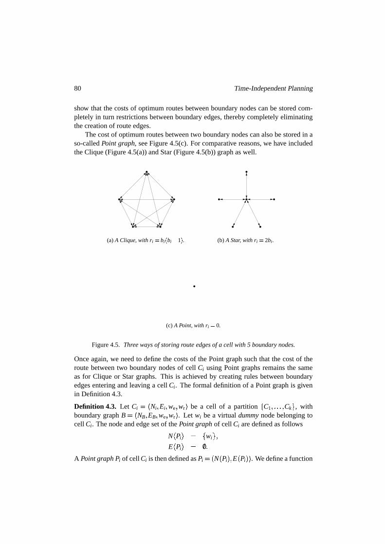
80 Time-IndependentPlanning
show that thecostsof optimumroutesbetweenboundarynodescanbestoredcom-pletely in turn restrictionsbetweenboundaryedges,therebycompletelyeliminatingthecreationof routeedges.
Thecostof optimumroutesbetweentwo boundarynodescanalsobestoredin aso-calledPoint graph, seeFigure4.5(c).For comparative reasons,we have includedtheClique(Figure4.5(a))andStar(Figure4.5(b))graphaswell.
(a) A Clique, with r i å bi æ bi ç 1è . (b) A Star, with r i å 2bi .
(c) A Point, with r i å 0.
Figure4.5. Threewaysof storingrouteedgesof a cell with 5 boundarynodes.
Onceagain,we needto definethecostsof thePointgraphsuchthat thecostof theroutebetweentwo boundarynodesof cell Ci usingPoint graphsremainsthe sameasfor Clique or Stargraphs.This is achieved by creatingrulesbetweenboundaryedgesenteringandleaving a cell Ci . Theformal definitionof a Pointgraphis givenin Definition4.3.
Definition 4.3. Let Ci É~Ê Ni Í Ei Í we Í wr Ì be a cell of a partition Õ C1 Í Î Î Î�Í Ck Ö , withboundarygraphB É�Ê NB Í EB Í we Í wr Ì . Let wi bea virtual dummynodebelongingtocellCi . Thenodeandedgesetof thePoint graphof cellCi aredefinedasfollows
N Ê Pi Ì É Õ wi Ö ÍE Ê Pi Ì É /0 Î
A Point graphPi of cellCi is thendefinedasPi É�Ê N Ê Pi Ì�Í E Ê Pi Ì Ì . Wedefineafunction

4.1 RepresentingRouteGraphs 81
dn : NB ü N thatgivesfor eachnodeu in NB thecorrespondingdummynodewi. Wesetdn Ê uÌ É wi for every u Ù Ni × NB. Furthermore,we definesomeadditionalruleson boundarygraphB usingu1 É δ1 Ê e1 Ì , u2 É δ2 Ê e1 Ì , v1 É δ1 Ê e2 Ì andv2 É δ2 Ê e2 Ìwr Ê e1 Í e2 Ì É ý wÚp Ê Ci Ý B Í u1 Í v2 Ì Ë we Ê e1 Ì Ë we Ê e2 Ì if dn Ê u2 Ì É dn Ê v1 Ì É wi ;
0 otherwiseÎFurthermore,endnodesu of boundaryedgeswith u Ù Ci needto bemodified.First,we definetwo functionsδo
1 : EB ü N andδo2 : EB ü N thatgive theoriginal startand
endnodeof a boundaryedgee respectively. Wesetδo1 Ê eÌ É δ1 Ê eÌ andδo
2 Ê eÌ É δ2 Ê eÌfor everye Ù EB. Now, wecanmodify theendnodesu of boundaryedgeswith u Ù Ci.Wesetδ j Ê eÌ É dn Ê δ j Ê eÌ Ì for all e Ù EB with δ j Ê eÌÙ Ci, j É 1 Í 2. Û
(a) A cell. (b) Thecell contractedinto a Point.
Figure4.6. Contractinga cell into a singlenode.
By usingPoint graphs,we contracta cell into a singlenode,seeFigure4.6. UsingRi É Pi andthemodifiedboundarygraph,thesearchgraphfor startnodes anddes-tinationd is givenby GS Ê sÍ d Ì . Again,we have thatbetweenevery pair of boundarynodesu, v, theminimumroutecostis equalto wÚp Ê Ci Í u Í vÌ asit is in theCliqueandStargraph.This is formally statedin thenext lemma.
Lemma 4.3. Letu andv betwoboundarynodeswith u Í v Ù NB û Ni adjacentto nodesin Ci . There existsa route p from u to v in B Ý Ki with costat mostc if andonly ifthere is a routepÜ fromu to v in B Ý Pi with costat mostc.Proof. “ à ” Assumethereexistsaroutep É Ó e1 Í p1 Í e2 Ô fromu É δ1 Ê e1 Ì to v É δ2 Ê e2 Ìin B Ý Ki with cost c. We have c É we Ê e1 Ìþâ we Ê e2 Ìþâ wÚp Ê Ci Ý B Í u Í vÌ Ë we Ê e1 Ì Ëwe Ê e2 Ì É wÚp Ê Ci Ý B Í u Í vÌ . Sincedn Ê δ2 Ê e1 Ì Ì É dn Ê δ1 Ê e2 Ì Ì=Ù Ci thereexists a routep É Ó e1 Í e2 Ô in B Ý Pi from u to v. This routehascostwe Ê e1 Ì3â we Ê e2 Ì3â wr Ê e1 Í e2 Ì Éwe Ê e1 Ì8â we Ê e2 Ì8â wÚp Ê Ci Ý B Í u Í vÌ Ë we Ê e1 Ì Ë we Ê e2 Ì É wÚp Ê Ci Ý B Í u Í vÌ É c.“ ä ” We know thatevery feasibleroute pÜ in B Ý Pi consistsof only two edges.LetpÜ É Ó e1 Í e2 Ô , with δ1 Ê e1 Ì É u, δ2 Ê e2 Ì É v, and δ2 Ê e1 Ì É δ1 Ê e2 Ì É wi from u to vwith costc in B Ý Pi. Wehave c É we Ê e1 Ì3â we Ê e2 Ì3â wr Ê e1 Í e2 Ì É we Ê e1 Ì8â we Ê e2 Ì8âwÚp Ê Ci Ý B Í u Í vÌ Ë we Ê e1 Ì Ë we Ê e2 Ì É wÚp Ê Ci Ý B Í u Í vÌ . Sothereexistsa routefrom u tov in B Ý Ki with costc. Û

82 Time-IndependentPlanning
From Lemma4.3, it follows that Theorem4.1 remainsvalid for Ri É Pi. It is nolongernecessaryto createpartitionsin sucha way thatrulesareonly formulatedoninternaledges,in orderto guaranteethatoptimumroutescanbeplanned.This is dueto thefactthatwe storetheoptimumroutecostof theroutefrom δ1 Ê e1 Ì to δ2 Ê e2 Ì aswr Ê e1 Í e2 Ì for dn Ê δ2 Ê e1 Ì Ì É dn Ê δ1 Ê e2 Ì Ì . However, we do not changeour partitioningalgorithm to take this into accountin order to be able to changethe route graphscreatedfor a partition from onetype to another. This meansthat for all partitions,only ruleson internaledgesexist. If we let go of therequirementthatrulesareonlyformulatedon internaledges,thenthepartitioningalgorithmscanbesimplified,thecomputationtime reducesandthequalityof thefoundpartitionsincreases.
Table 4.2 gives for all threeroute graphsthe numberof rules that needto becreated.In thesecondcolumnthenumberof ruleswith apositive finite costis given.In thethird columnthetotal numberof ruleswith a positive costis given. Notethatit is possibleto storeonly theruleswith a positive finite costandstill planoptimumfeasibleroutes. All rules with infinite costs(in a route graph)can be taken intoaccountby lettingarouteplanningalgorithmonly returnedgesthatleadto afeasibleroute when it determinesall adjacentedgesof an edgee. Note that the last rowindicatesthenumberof rulesfor Pointgraphsfor partitionsthatdo not requirethatrulesareonly formulatedonpairsof internaledges.
Routegraph Numberof finite rules Total numberof rules
Clique 0 bi Ê bi Ë 1Ì 2Star bi Ê bi Ë 1Ì bi Ê bi â 1ÌPoint ØEB Ê Ci ÌWØ Ê ØEB Ê Ci ÌWØ Ë 1Ì ØEB Ê Ci ÌWØ Ê ØEB Ê Ci ÌWØ Ë 1ÌPointÜ ØEB Ê Ci ÌWØ 2 ØEB Ê Ci ÌWØ 2
Table4.2. Numberof rulesfor differentroutegraphs.
Note that from Table4.2 we canseethat thestoragerequirements(edgesandfiniterulescombined)areof thesameorderfor eachof thethreeroutegraphs.
In real-world roadnetworksalsoturn restrictionson pairsof non-adjacentedgesexist, which we canformulateby usingwr : P Ê GÌ ü/ÿ ë0 Ý ∞. Considerfor examplethe intersectionin Figure4.7(a). A restrictionto make a U-turn (for instancea turnfrom edgee1 to edgee6) canbe formulatedaswr Ê e1 Í e2 Í e11 Í e5 Í e6 Ì É ∞. Note thattheintroductionof wr Ê e2 Í e11 Ì É ∞ wouldalsocauseroutesthatmakealeft turn frome1 to e12 to be illegal. Suchcomplex turn restrictionson non-adjacentedgescanbe handledby creatingPoints. If the destinationnodeis a nodeother thannodes1 Í Î Î Î�Í 4 thenwe can replacenodes1 Í Î Î Î�Í 4 andedgese2 Í e5 Í e8 Í e11 by a Point, seeFigure 4.7(b). The rules betweenedgesenteringand leaving the intersection(orPoint)canbeusedto guaranteethatonly legal routesareplanned,andthatthepropercostsareused.
Notethatalsootherroutegraphsarepossible,for exampleaRingasin Figure4.8.

4.2 Algorithmsfor Time-IndependentOptimumRoutePlanning 83
1 2
3 4
e1
e9
e2
e3
e11e12
e5
e8
e6
e7
e4
e10
(a) An intersection.
e1
e9
e3
e12
e6
e7
e4
e10
(b) An intersectionasPoint graph.
Figure4.7. Formulatingan intersectionasa Point.
This structurehastheadvantagethatthedegreeof all nodesis three.However, it re-quirestheintroductionof rulesformulatedonnon-adjacentedges,whichcomplicatestherouteplanningalgorithm.
Figure4.8. Analternativewayof storingtherouteedgesof a cell: theRing.
4.2 Algorithms for Time-IndependentOptimum Route Planning
This sectiondiscussesthe planningof optimumtime-independentroutesin single-level partitions. In Section2.1 we motivatedandexplainedthe useof rules. Rulesareusedto representfor instanceforbiddenturnsin a roadgraph.Theserulesinflu-encetheplanningof optimumroutes.Becauseforbiddenturnsmaybe presentin aroadgraph,an optimumroute in a roadgraphmay containa nodemore thanonce.Considertheexamplein Figure4.9, andassumethatwr Ê e1 Í e2 Ì É ∞. Theoptimumroutefrom node1 to node6 is theroutethroughall six nodes,which passesthroughnode2 twice. Note that this cyclic route is the only feasibleroutefrom node1 tonode6.
Becauseanoptimumroutemaycontaina nodemorethanonce,a standardnode

84 Time-IndependentPlanning
1
2
34
5 6
e1
e2
Figure4.9. Anoptimumroutewith a cycle.
labelling algorithm suchas the standardAÚ -algorithm [Hart, Nilsson & Raphael,1968]cannotbeusedto determinetheoptimumroute. However, anoptimumroutedoesnot containan edgemore than once. In order to plan optimum routesin agraphwith rules,amodifiedAÚ -algorithmcanbeusedthatevaluatesedgesinsteadofnodes.Schmid[2000] andWinter [2002] considerturn restrictionson pairsof adja-centedges.Both paperspresentpolynomial-timealgorithmsthatconstructoptimumroutesthatmaycontainnodesmorethanonce.Winter [2002] usesthatanoptimumroutedoesnot containanedgemorethanonceby constructingtheline graphof theroadgraphto plan optimumroutes. Szeider[2003] considersthe problemof deter-miningwhetherasimplepathexistsbetweentwo nodesin anundirectedsimplegraphwith turn restrictions,wherea simplepathis a routein which eachnodeappearsatmostonce.He provesthat this problemis NP-completeif thegraphsatisfiescertainconditions.
We usealgorithmCÚ definedin Figure4.10to determineanoptimumroutein a(partitioned)roadgraphG with rules.Algorithm CÚ is a modifiedAÚ -algorithm.TheAÚ -algorithmis ashortestpathalgorithmthatis basedon Dijkstra’s algorithm[Dijk-stra,1959]. In orderto reducethenumberof evaluatededges,theAÚ -algorithm[Hart,Nilsson & Raphael,1968] usesan estimationof the cost from a nodeto the des-tination, which is called the h-value. The minimum cost from the start nodeto anodeis calledtheg-value.TheAÚ -algorithmselectsa nodewith minimumexpectedcost from the startnodeto the destination,i.e. a nodewith minimum g â h-value.Subsequently, all the adjacentnodesof the selectednodearedeterminedandtheirminimum expectedcostsareupdated.The processis repeateduntil no betterroutefrom startnodes to destinationnoded canbe found. As explaineda modifiedAÚ -algorithm[Hart, Nilsson& Raphael,1968]canbeusedto plananoptimumrouteina roadgraphwith turn restrictions.Becauseof theseturn restrictions,we selecttheedgewith minimumexpectedcostfrom thestartnodeto thedestination.

4.2 Algorithmsfor Time-IndependentOptimumRoutePlanning 85
Our CÚ -algorithmstartsby settingall costsequalto infinity, the setof unevaluatededgesequalto theedgesetof theinputgraph,andtherouteequalto theemptyroute.No edgehasa predecessoryet. Furthermore,the costof the routefrom startnodes to startnodes is setto 0, thecostsof theedgesadjacentto startnodes aredeter-mined,andtheirpredecessorsareset.Subsequently, thealgorithmrepeatedlyselectstheedgee from thesetof unevaluatededgesH with minimumexpectedcostto thedestination(i.e. minimumg â h-value),anddeterminesall allowedadjacentedgesofedgee. Thecostsandpredecessorsof theseedgesareupdatedif theminimumfoundroutecostchanges.Thenedgee is removed from the setof unevaluatededgesH.This processcontinuesuntil theminimumroutecostfrom startnodes to destinationd is foundor until thesetof evaluatededgesH is empty. If theoptimumroutecostisfoundthealgorithmdeterminesthematchingrouteby usingthestoredpredecessors,otherwisethealgorithmreturnstheemptyrouteandaninfinite cost.
The AÚ -algorithm can be usedto plan optimum routesif the h-value under-estimatesthe real cost from the currentnodeto the destination,and if the h-valueis a so-calleddualfeasibleestimator.Algorithm CÚ alsousesa dualfeasibleestima-tor h to direct theplanningprocessto thedestination.Recallthedefinitionof a dualfeasibleestimator, seePearl[1984].
Definition 4.4. A functionh : N üEÿ is calledadualfeasibleestimatorfor roadgraphG if we Ê eÌ'á h Ê δ1 Ê eÌ Ì Ë h Ê δ2 Ê eÌ Ì for every edgeeof roadgraphG. ÛThis definitioncanbeeasilygeneralizedto estimatorsfor edges,asfollows.
Definition 4.5. A functionh : E ü ÿ is calledadualfeasibleestimatorfor roadgraphG if we Ê e2 Ì'á h Ê e1 Ì Ë h Ê e2 Ì Ë wr Ê e1 Í e2 Ì for all edgese1 Í e2 of roadgraphG suchthatδ2 Ê e1 Ì É δ1 Ê e2 Ì . ÛPearl[1984] provesthata permanentlabelsetby a nodelabellingalgorithmis nevermodified if the expectedremainingcost from a nodeu to destinationd is a dualfeasibleestimator. Thiscanbeeasilygeneralizedto roadgraphswith turnrestrictions.Notethat in ourCÚ -algorithma labelg Ê eÌ of edgee becomespermanentwhenedgee is selectedfrom setH.
Lemma 4.4. LetG bea roadgraph. A permanentlabel setbyCÚ is nevermodifiedifa dual feasibleestimatoris used.Proof. Note that becauseroadgraphG containsrules,we have to evaluateedgesinsteadof nodes.Sosupposeanedgee2 with apermanentlabel
� Ê e2 Ì hasbeenfoundby thealgorithmthat now receivesa lower cost. Thenthe new label of e2 is lowerthantheold one,so
� Ê e1 ÌHâ we Ê e2 ÌHâ wr Ê e1 Í e2 Ì�� � Ê e2 Ì , with e1 É λ Ê e2 Ì in algorithmCÚ . Becauseedgee2 waspermanent,weknow
� Ê e2 Ì�â h Ê e2 Ì)ã � Ê e1 Ì�â h Ê e1 Ì . Becauseh Ê eÌ is adualfeasibleestimator,
� Ê e2 Ì Ë � Ê e1 Ì'ã h Ê e1 Ì Ë h Ê e2 Ì"ã we Ê e2 ÌHâ wr Ê e1 Í e2 Ì .This is a contradictionwith we Ê e2 Ì!â wr Ê e1 Í e2 Ì�� � Ê e2 Ì Ë � Ê e1 Ì . So the label of e2
cannothave beenpermanent.Therefore,apermanentlabelis never modified. Û

86 Time-IndependentPlanning
Algorithm C�Input: A roadgraphG, startnodes, destinationnoded.
H : Thesetof unexpandededges.g æ eè : Theminimumfoundcostof a routefrom nodes to edgee.gn æ uè : Theminimumfoundcostof a routefrom nodes to nodeu.λ æ eè : Theadjacentedgeleadingto edgee of theminimum-costroutefrom s to e.p : Theminimum-costroutefrom s to d.w�p æ pè : Thecostof routep.h æ uè : Theestimatedcostfrom nodeu to noded.h æ eè : Theestimatedcostfrom edgee to noded.
Initialization stepH å E, p å��� , w�p æ pè å ∞for everye H do
g æ eè å ∞λ æ eè å /0
end forfor everyu N do gn æ uè å ∞ end forgn æ sè å 0for everye H suchthatδ1 æ eè å s do
g æ eè å we æ eèλ æ eè å e
end for
Main body of the algorithmwhile thereis anedgee H with gn æ d è�� g æ eè� h æ eè do
Let e beanedgefrom H with g æ eè� h æ eè minimumfor everyallowedadjacentedgee1 of e in G do
if g æ e1 è�� g æ eè� we æ e1 è� wr æ e� e1 è theng æ e1 è å g æ eè� we æ e1 è� wr æ e� e1 ègn æ δ2 æ e1 è�è å min � gn æ δ2 æ e1 è�è�� g æ e1 è��λ æ e1 è å e
end ifend forH å H ��� e�
endwhileif gn æ d è�� ∞ then w�p æ pè å g æ eè and constructoptimumroutep from edgee usingλ æ eè end if
Output: Optimumroutep, andtheminimumroutecostw�p æ pè .Figure4.10. AlgorithmC� .

4.2 Algorithmsfor Time-IndependentOptimumRoutePlanning 87
In algorithmCÚ , we usethat theusedestimatoris dual feasible.NotethatalgorithmCÚ canalsobe usedfor unpartitionedroadgraphs,by regardingthe roadgraphasasingle cell, and the boundarygraphas the empty graph. The time-complexity ofalgorithmCÚ doesnot dependon the numberof rules,but only on the numberofedges.Specifically, algorithmCÚ canbeimplementedin O Ê n â mlogmÌ similarly toalgorithmAÚ , asstatedin Theorem4.2.
Theorem 4.2. AlgorithmCÚ canbeimplementedwith a worst-casetime-complexityof orderO Ê n â mlogmÌ , wheren andmdenotethenumberof nodesandedgesin thesearchgraphrespectively.Proof. AlgorithmCÚ is identicalto algorithmAÚ upto thefactthatedgesareselectedin eachstep,andupto thedeterminationof thecostwr Ê e1 Í e2 Ì for every two adjacentedgese1 ande2. Notethatwe canchoosewr Ê e1 Í e2 Ì in suchaway thatthereexistsatmostonerulecostbetweeneverypairof adjacentedges.Theselectionof anadjacentedgee2 of edgee1 andthedeterminationof thecostwr Ê e1 Í e2 Ì canbedonein asingleoperation.This canbeachievedby storingfor eachedgee1 for every adjacentedgea datastructurecontaining(a referenceto) theadjacentedgee2 and(a referenceto)thecostwr Ê e1 Í e2 Ì . Therefore,thetime-complexity of algorithmCÚ doesnot dependon the numberof rules,but only on the numberof edges.The proof now followsimmediatelyfrom the fact that the AÚ -algorithmcanbe implementedwith a worst-casetime-complexity of orderO Ê n â mlognÌ , see[Johnson,1972], wheren andmdenotethenumberof nodesandedgesin thesearchgraphrespectively. ÛTo plan an optimum route with the CÚ -algorithm, we usea h-value basedon theEuclideandistancefrom anodeto thedestination.For anodewith ageographicallo-cationassociatedwith it, theEuclideandistanceto thedestinationcanbedetermined.Becausewe areconcernedwith real-world roadnetworks, every nodein the road-graphhasa geographicallocation. We canusetheEuclideandistanceash-valueiftheedgecostsareequalto thelengthof theedge.For edgecostsequalto thedrivingtime, theEuclideandistancedivided by theoverall maximumspeedcanbeusedash-valueto planoptimumroutes.Note that this appliesto theh-valuefor bothedgesandnodes.
If aCliqueis usedasroutegraph,every nodein thesearchgraphhasageograph-ical location,so algorithmCÚ in Figure4.10 canbe usedto plan optimumroutes.Whenwe needto plana routein a searchgraphthatis constructedwith Staror Pointgraphs,anaddeddummynodein a Staror Pointgraphdoesnot exist in reality andthereforehasno geographiclocation associatedwith it. Without a geographiclo-cation, the remainingEuclideandistanceis not defined,and thereforethe h-valuecannotbecomputedfor thesedummynodes.We first definetheh-valuefor anedgeendingwith adummynode,andthenweshow thatthis canbeusedto planoptimumroutesin asearchgraphthatcontainsStargraphs,seealso[Flinsenberg, 2003b].

88 Time-IndependentPlanning
Definition 4.6. Let GS É�Ê N Í E Í we Í wr Ì be a searchgraphthat containsStargraphsanddummynodesU . Let h Ê uÌ denotethe expectedremainingcost from nodeu ÙN û U to destinationd Ù N û U .
DefinehÚ Ê eÌ É ý h Ê δ1 Ê eÌ Ì Ë we Ê eÌ if δ2 Ê eÌ'Ù U ;h Ê δ2 Ê eÌ Ì if δ2 Ê eÌ ñÙ U Î Û
Theh-valueof edgee is equalto theexpectedremainingcostfrom theendnodeoftheedgeto thedestination.If h Ê uÌ under-estimatestheremainingcostthenhÚ Ê eÌ alsounder-estimatestheremainingcostbecausetheremainingcostfrom theend-nodeofe with δ2 Ê eÌqÙ U , is equalto the remainingcostfrom δ1 Ê eÌ minusthecostof edgee, we Ê eÌ . Furthermore,we canshow that theestimatordefinedin Definition 4.6 is adualfeasibleestimator.
Lemma 4.5. Let G bea roadgraph with dummynodesU. If h Ê uÌ is a dual feasibleestimatorfor roadgraphG û U, thenhÚ Ê eÌ is a dual feasibleestimatorfor roadgraphG.Proof. Assumeestimatorh Ê uÌ isdualfeasiblefor G û U , whichmeansthath Ê δ1 Ê eÌ Ì Ëh Ê δ2 Ê eÌ Ì"ã we Ê eÌ for everye Ù G û U . BecausehÚ Ê eÌ É h Ê δ2 Ê eÌ Ì for everyδ2 Ê eÌ ñÙ U ,we know that for every adjacente1 Í e2 Ù G û U the condition in Definition 4.5 issatisfied.Now let e besuchthat δ1 Ê eÌKÙ G û U andδ2 Ê eÌqÙ U . Becauseδ2 Ê eÌqÙ U ,let e1 be an edgewith δ2 Ê e1 Ì É δ1 Ê eÌ andδ1 Ê e1 Ì�Ù G û U . We needto prove thatwe Ê eÌIâ wr Ê e1 Í eÌIâ hÚ Ê eÌ�á hÚ Ê e1 Ì . Becauseno rulesexist betweenedgese1 ande,wehavewe Ê eÌ â wr Ê e1 Í eÌUâ hÚ Ê eÌ Ë hÚ Ê e1 Ì É we Ê eÌUâ h Ê δ1 Ê eÌ Ì Ë we Ê eÌ Ë h Ê δ1 Ê eÌ Ì)á 0.Now let e be suchthat δ1 Ê eÌ�Ù U andδ2 Ê eÌqÙ G û U . Becauseδ1 Ê eÌ�Ù U , let e1 bean edgewith δ2 Ê e1 Ì É δ1 Ê eÌ and δ1 Ê e1 Ì�Ù G û U . We needto prove that we Ê eÌ.âwr Ê e1 Í eÌ@â hÚ Ê eÌ�á hÚ Ê e1 Ì . We have we Ê eÌ@â wr Ê e1 Í eÌ.â hÚ Ê eÌ Ë hÚ Ê e1 Ì É we Ê eÌ.âwr Ê e1 Í eÌ3â h Ê δ2 Ê eÌ Ì Ë h Ê δ1 Ê e1 Ì Ì8â we Ê e1 Ì . Becauseh Ê uÌ is a dual feasibleestimator,we know thath Ê δ1 Ê e1 Ì Ì Ë h Ê δ2 Ê eÌ Ìã we Ê e1 Ì8â we Ê eÌ . This giveswe Ê eÌ3â wr Ê e1 Í eÌ8âh Ê δ2 Ê eÌ Ì Ë h Ê δ1 Ê eÌ Ì�â we Ê e1 Ì)á we Ê eÌUâ wr Ê e1 Í eÌ Ë we Ê e1 Ì Ë we Ê eÌ�â we Ê e1 ÌCá 0. ThisprovesthathÚ Ê eÌ is adualfeasibleestimator. ÛFrom Lemma4.4 andLemma4.5 it follows that we canagainusealgorithmCÚ inFigure4.10to planoptimumroutesin asearchgraph,by usingh Ê eÌ in Definition4.6,whererouteedgesarestoredin Stargraphs.
Whenwe needto plan a route in a searchgraphthat is constructedwith Pointgraphs,we canagainusealgorithmCÚ in Figure4.10. Note that an adjacentedgee1 of edgee Ù B in algorithmCÚ is anedgewith dn Ê δ2 Ê eÌ Ì É dn Ê δ1 Ê e1 Ì Ì . Thevalueof h Ê eÌ canbe determinedfor e Ù B by consideringthe endnodeof edgee in theboundarygraph,δo
2 Ê eÌ , and not by looking at dn Ê δ2 Ê eÌ Ì . Definition 4.7 gives theformaldefinitionof theestimatedremainingcostto thedestinationfor asearchgraphcontainingPoints.

4.3 ComputationalEvaluation 89
Definition 4.7. Let GS É�Ê N Í E Í we Í wr Ì bea searchgraphthat containsPointgraphsand dummy nodesU . Let h Ê uÌ denotethe expectedremainingcost from a nodeu Ù N û U to destinationd Ù N û U .
DefinehÜ Ê eÌ É ý h Ê δo2 Ê eÌ Ì if δ2 Ê eÌÙ U ;
h Ê δ2 Ê eÌ Ì if δ2 Ê eÌ ñÙ U Î ÛTheestimatordefinedin Definition 4.7 is dualfeasibleasstatedin Lemma4.6.
Lemma 4.6. Let P bea partition Õ C1 Í Î Î Î�Í Ck Ö with boundarygraphB of roadgraphG. Let GS bea searchgraph of P containingdummynodesU andPoints. If h Ê uÌ isa dual feasibleestimatorfor searchgraphGÜS of P containingCliques,thenhÜ Ê eÌ is adual feasibleestimatorfor searchgraphGS.Proof. Assumeestimatorh Ê uÌ is dual feasiblefor GÜS containingCliques.We knowfrom Definition4.4h Ê δ1 Ê eÌ Ì Ë h Ê δ2 Ê eÌ ÌKã we Ê eÌ for every e Ù GS û U ,h Ê δo
1 Ê eÌ Ì Ë h Ê δo2 Ê eÌ ÌKã we Ê eÌ for every ewith δ1 Ê eÌÙ U or δ2 Ê eÌÙ U ,
h Ê δo2 Ê e1 Ì Ì Ë h Ê δo
1 Ê e2 Ì Ìqã wr Ê e1 Í e2 Ì Ë we Ê e1 Ì Ë we Ê e2 Ì , for every adjacente1 Í e2 withδ2 Ê e1 Ì�Í δ1 Ê e2 Ì'Ù U .Let e1, e2 be two (adjacent)edgeswith δ1 Ê e2 Ì É δ2 Ê e1 Ì . We needto prove thatwe Ê e2 Ì8â wr Ê e1 Í e2 Ì8â hÜ Ê e2 Ì'á hÜ Ê e1 Ì . BecausehÜ Ê eÌ É h Ê δ2 Ê eÌ Ì for every δ2 Ê eÌ ñÙ U ,theconditionin Definition4.5 is satisfiedfor every adjacente1 Í e2 Ù G û U .For δ1 Ê e2 Ì É δ2 Ê e1 Ì"Ù U andδ2 Ê e2 Ì"Ù U we havewe Ê e2 Ì3â wr Ê e1 Í e2 ÌHâ hÜ Ê e2 Ì Ë hÜ Ê e1 Ì É we Ê e2 Ì3â wr Ê e1 Í e2 ÌHâ h Ê δo
2 Ê e2 Ì Ì Ë h Ê δo2 Ê e1 Ì Ì É
we Ê e2 Ì8â wr Ê e1 Í e2 Ì8â h Ê δo2 Ê e2 Ì Ì Ë h Ê δo
1 Ê e2 Ì Ì8â h Ê δo1 Ê e2 Ì Ì Ë h Ê δo
2 Ê e1 Ì Ì'áwe Ê e2 Ì8â wr Ê e1 Í e2 Ì Ë we Ê e2 Ì Ë wr Ê e1 Í e2 Ì3â we Ê e1 Ì8â we Ê e2 Ì"á 0.For δ1 Ê e2 Ì É δ2 Ê e1 Ì ñÙ U andδ2 Ê e2 Ì"Ù U we havewe Ê e2 Ì3â wr Ê e1 Í e2 ÌHâ hÜ Ê e2 Ì Ë hÜ Ê e1 Ì É we Ê e2 Ì3â wr Ê e1 Í e2 ÌHâ h Ê δo
2 Ê e2 Ì Ì Ë h Ê δ2 Ê e1 Ì Ì Éwe Ê e2 Ì8â wr Ê e1 Í e2 Ì8â h Ê δo
2 Ê e2 Ì Ì Ë h Ê δo1 Ê e2 Ì Ì'á we Ê e2 Ì3â wr Ê e1 Í e2 Ì Ë we Ê e2 Ì"á 0.
For δ1 Ê e2 Ì É δ2 Ê e1 Ì"Ù U andδ2 Ê e2 Ì ñÙ U we havewe Ê e2 Ì3â wr Ê e1 Í e2 ÌHâ hÜ Ê e2 Ì Ë hÜ Ê e1 Ì É we Ê e2 Ì3â wr Ê e1 Í e2 ÌHâ h Ê δ2 Ê e2 Ì Ì Ë h Ê δo
2 Ê e1 Ì Ì Éwe Ê e2 Ì8â wr Ê e1 Í e2 Ì8â h Ê δo
2 Ê e2 Ì Ì Ë h Ê δo1 Ê e2 Ì Ì8â h Ê δo
1 Ê e2 Ì Ì Ë h Ê δo2 Ê e1 Ì Ì'á
we Ê e2 Ì8â wr Ê e1 Í e2 Ì Ë we Ê e2 Ì Ë wr Ê e1 Í e2 Ì3â we Ê e1 Ì8â we Ê e2 Ì"á 0.This provesthathÜ Ê eÌ is adualfeasibleestimator. ÛFrom Lemma4.4 and Lemma4.6 it follows that we can againusealgorithmCÚin Figure 4.10 to plan optimum routesin a searchgraph,by using estimatorhÜ inDefinition 4.7,whererouteedgesarestoredin Pointgraphs.
4.3 Computational Evaluation
In thissection,wecomparetheplanningof optimumroutesin roadgraphsfor all threemethodsof storingrouteedges,discussedin Section4.1.1,4.1.2and4.1.3.Observethatthenumberof edgesin aCliquegraphis largerthanthenumberof edgesin aStar

90 Time-IndependentPlanning
graphif bi á 4. For bi É 3 thenumberof edgesin aStargraphis equalto thenumberof edgesin a Clique graph,while for bi ã 2 thenumberof edgesin a Stargraphislarger thanthenumberof edgesin a Cliquegraph.We chooseto createa Stargraphfor cellswith bi á 4 anda Cliquegraphfor cellswith bi ã 3. For bi É 3, we createa Cliquegraphbecausethis structureis intuitively clearer, andrequiresfewer nodesandfinite turn restrictionsto bestored.
We usedthe partitionscreatedby the Merging-Algorithm. Dataon theseparti-tionscanbe found in Table3.5,andin AppendixC. We have planned2,000routesthroughtheNetherlandsbetweenstartanddestinationnodesthatareselectedin suchawaythatthey arebelievedtoberepresentative for theroutesdrivenbyatypicalcom-muter. Table4.3givessomeadditionalinformationon theroutesthatwereplanned.For every selectednode(4,000startor destinationnodes)Table4.3 indicatesif it islocatedin anurbanor ruralarea.Wedeterminedthesetof 2,000startanddestinationnodesby selectingedgesandchoosingoneof theendnodesof theselectededgeasstartor destinationnode.
Distribution of Elements Number PercentageNumberof routes - 2,000 100%Urban/Rural Urban 2,063 51%
Rural 1,937 49%Euclidean 0 to 1,000 2 0%distance(m) 1,000 to 2,500 5 0%
2,500 to 5,000 10 0%5,000 to 10,000 49 2%
10,000 to 25,000 285 14%25,000 to 50,000 808 40%50,000 to 100,000 306 15%
100,000 to 250,000 509 25%250,000 to 500,000 26 1%500,000 to 1,000,000 0 0%
morethan 1,000,000 0 0%
Table4.3. Selectedstart anddestinationpairs in theNetherlands.
The setof selectedstartanddestinationnodescoversthe entirecountry, ascanbeseenfrom Figure4.11. Sowe cansafelybaseour evaluationof algorithmCÚ on theselectedpairsof startanddestinationnodes.Wewill alsoreferto thissetasour routebatch.
Tables4.4and4.5give theresultsfor planningthese2 Í 000routeswhentheedgecostsaregivenby thetimeneededto traversetheedgeatthemaximumallowedtravelspeedandby the edgelength respectively. Note that the maximumallowed travelspeedis different for different typesof edges,for examplethe maximumallowed

4.3 ComputationalEvaluation 91
Figure4.11. Startanddestinationnodesin theNetherlandsfromTable4.3.
travel speedof a motorway edgeis assumedto be 120 km/h. We refer to a routewith minimum travel time as a fastestroute, and to a route with minimum routelengthasa shortestroute. Column1 in Tables4.4 and4.5 givesthe roadnetworkusedfor planningthe routes. Column2 givesthe numberof edgesthat is selectedfrom thesetof unexpandededgesH of algorithmCÚ in Figure4.10for unpartitionedroadnetworks,or equivalently, thenumberof evaluatededges.Column3 givesthevalueof r i thatwasusedto createa partition. Columns4, 5 and6 give thenumberof evaluatededgesfor a partitionedroadgraph,usingClique,StarandPoint graphsrespectively to storetherouteedges.In the“Star”-column,Cliquegraphsarecreatedfor cellswith bi ã 3.
Furthermore,we have also gathereddataon the type of the evaluatededges.Specifically, we determinedfor eachevaluatededgewhetherthis edgewasan in-ternal edge,or a boundaryor route edge. For eachinternal edgewe determinedwhetherit waslocatedin thecell containingthe startnodeor thedestinationnode.Thisdatacanbefoundin Tables4.6and4.7.Againcolumn1 givestheusedroadnet-work. Column2 givesthevalueof r i thatwasusedto createapartition.Thecolumnsdenotedby C Ê sÌ presentthepercentageof evaluatededges,for which theevaluatededgeis locatedin thecell containingthestartnode.Similarly, thecolumnsdenotedby C Ê d Ì presentthe percentageof evaluatededges,for which the evaluatededgeislocatedin thecell containingthedestinationnode.Finally, thecolumnsdenotedby Bpresentthepercentageof evaluatededges,for whichtheevaluatededgeis aboundaryor routeedge.All percentagesareroundedto thenearestinteger.
As canbe seenfrom Table4.4 andTable4.5, thenumberof evaluatededgesislowestif therouteedgesarestoredin Pointgraphs.Thenumberof evaluatededgesis highestif the routeedgesarestoredasClique graphs.This canbe explainedbylookingat thenumberof edgesin theroutegraph.Thesearchgraphusedfor planning

92 Time-IndependentPlanning
Map(Edges) AÚ r i Clique Star Point
Sophia 1,261 rCi 294 277 200
(2,015) rSi 300 277 195
rPi 413 330 167
Eindhoven 6,822 rCi 2,346 1,159 643
(14,696) rSi 2,553 1,229 617
rPi 3,235 1,593 655
Siegen 14,409 rCi 2,518 1,545 1,107
(23,953) rSi 2,905 1,520 889
rPi 3,285 1,739 824
Giesen/Wetzlar 43,220 rCi 5,540 3,052 2,249
(88,177) rSi 5,697 2,770 1,605
rPi 6,892 3,167 1,455
Antwerp 42,459 rCi 8,665 5,463 4,852
(98,564) rSi 11,096 3,656 2,037
rPi 13,725 4,321 1,892
Netherlands 340,420 rCi 36,588 19,004 17,404
(1,135,280) rSi 42,824 10,673 6,683
rPi 51,951 11,768 5,676
Table4.4. Averagenumberof evaluatededgesfor planningfastestroutes.

4.3 ComputationalEvaluation 93
Map(Edges) AÚ r i Clique Star Point
Sophia 1,179 rCi 276 263 192
(2,015) rSi 282 262 188
rPi 386 308 158
Eindhoven 6,680 rCi 2,311 1,114 626
(14,696) rSi 2,516 1,178 600
rPi 3,185 1,518 637
Siegen 13,564 rCi 2,391 1,479 1,079
(23,953) rSi 2,749 1,433 860
rPi 3,097 1,604 786
Giesen/Wetzlar 42,318 rCi 5,481 2,960 2,215
(88,177) rSi 5,627 2,644 1,578
rPi 6,798 2,990 1,425
Antwerp 40,183 rCi 8,308 5,283 4,720
(98,564) rSi 10,522 3,444 1,975
rPi 12,971 3,991 1,813
Netherlands 335,170 rCi 36,328 18,662 17,114
(1,135,280) rSi 42,520 10,451 6,576
rPi 51,486 11,490 5,585
Table4.5. Averagenumberof evaluatededgesfor planningshortestroutes.

94 Time-IndependentPlanning
Clique Star PointMap (Edges) r i C Ê sÌ B C Ê d Ì C Ê sÌ B C Ê d Ì C Ê sÌ B C Ê d ÌSophia rC
i 44 43 13 44 42 14 56 26 17(2.015) rS
i 43 44 13 44 43 13 56 26 17rPi 20 74 6 22 72 6 34 57 9
Eindhoven rCi 26 67 7 33 58 9 48 39 13
(14.696) rSi 21 73 6 27 66 7 42 47 11
rPi 12 85 3 15 82 4 26 68 6
Siegen rCi 37 52 11 47 39 14 61 21 18
(23.953) rSi 26 66 7 35 55 10 50 35 14
rPi 17 78 5 22 72 6 36 54 10
Giesen/Wetzlar rCi 37 52 10 50 35 14 64 18 18
(88.177) rSi 25 68 7 35 55 10 51 35 14
rPi 16 81 4 22 73 6 36 54 9
Antwerp rCi 51 37 13 67 17 16 74 8 18
(98.564) rSi 22 73 5 35 57 8 51 37 12
rPi 13 84 3 21 74 5 36 56 8
Netherlands rCi 54 30 16 69 10 20 74 4 22
(1.135.280) rSi 31 60 9 48 38 13 60 23 17
rPi 21 73 6 35 55 10 48 38 13
Table4.6. Distribution of theevaluatededgesfor planningfastestroutes.
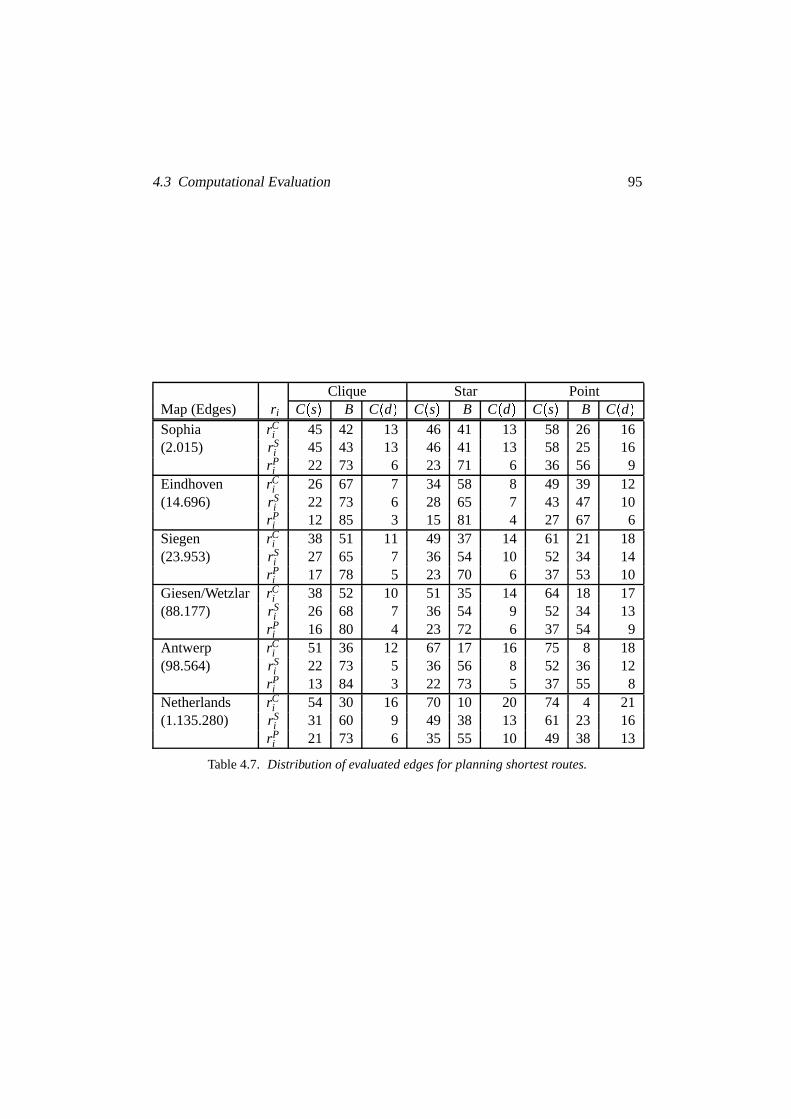
4.3 ComputationalEvaluation 95
Clique Star PointMap (Edges) r i C Ê sÌ B C Ê d Ì C Ê sÌ B C Ê d Ì C Ê sÌ B C Ê d ÌSophia rC
i 45 42 13 46 41 13 58 26 16(2.015) rS
i 45 43 13 46 41 13 58 25 16rPi 22 73 6 23 71 6 36 56 9
Eindhoven rCi 26 67 7 34 58 8 49 39 12
(14.696) rSi 22 73 6 28 65 7 43 47 10
rPi 12 85 3 15 81 4 27 67 6
Siegen rCi 38 51 11 49 37 14 61 21 18
(23.953) rSi 27 65 7 36 54 10 52 34 14
rPi 17 78 5 23 70 6 37 53 10
Giesen/Wetzlar rCi 38 52 10 51 35 14 64 18 17
(88.177) rSi 26 68 7 36 54 9 52 34 13
rPi 16 80 4 23 72 6 37 54 9
Antwerp rCi 51 36 12 67 17 16 75 8 18
(98.564) rSi 22 73 5 36 56 8 52 36 12
rPi 13 84 3 22 73 5 37 55 8
Netherlands rCi 54 30 16 70 10 20 74 4 21
(1.135.280) rSi 31 60 9 49 38 13 61 23 16
rPi 21 73 6 35 55 10 49 38 13
Table4.7. Distribution of evaluatededgesfor planningshortestroutes.

96 Time-IndependentPlanning
an optimumroutecontainsthemostedgesin the “Clique”-column,andthe leastinthe“Point”-column.
Furthermore,weseethatfor all roadnetworks,exceptfor thatof Eindhoven,it ispreferableto adjustthepartitioningcriteriumto thetypeof routegraphsthatwill becreatedfor thatpartition. Specifically, thenumberof evaluatededgesfor partitionsgeneratedwith r i É bi Ê bi Ë 1Ì is lowest if Cliquegraphsareusedto storethe routeedges.Similarly, if thepartitionis generatedwith r i É min Õ 2bi Í bi Ê bi Ë 1Ì Ö it is bestto useStar graphs(for cells with bi � 3) to storethe route edges. For partitionsgeneratedwith bi É 0, Point graphsshouldbe usedto storethe routeedges.Thiscanbeexplainedfrom thefactthatthepartitionsthataregeneratedusingaparticularvalue of r i , try to optimize the partition with the future route planningprocessinmind. If the partition is generatedusinga differentvalue for r i than the oneusedlater on, the numberof routeedgesin the searchgraphdoesnot correspondto theexpectedaveragenumberof routeedgesthat wascomputedduring the creationofthepartition. As a result,otherpartitionsresultin fasterrouteplanning,specificallythosepartitionsthatarecreatedusingthepropernumberof routeedgespercell.
The overall bestresultsareobtainedwith partitionsgeneratedwith r i É 0, andPoint graphsfor storingrouteedges.As canbe seenfrom Table4.4 andTable4.5,planningan optimumroutebetweentwo randomnodesin the roadnetwork of theNetherlands,with anaverageroutelengthof 122kilometers,requirestheevaluationof about5,500edges.
From Tables4.6 and4.7, we canseethat for partitionscreatedwith a decreas-ing valueof r i , a higherpercentageof theevaluatededgesconsistsof boundaryandroute edges. This is causedby the fact that thosepartitionstend to have smallercellsandmoreboundaryandrouteedges.Furthermore,for partitionswith Cliquesahigherpercentageof theevaluatededgesconsistsof boundaryandrouteedgesthanfor partitionswith Stars,for which in turn,ahigherpercentageof theevaluatededgesconsistsof boundaryandrouteedgesthanfor partitionswith Points.This is becausea Cliquecontainsmorerouteedgesthana Star, which hasmorerouteedgesthanaPointgraph.Actually, thepercentageof evaluatedboundaryedgescanbefoundin thesub-columnB of thecolumndenotedby Point. Theeffect of creatinga Starinsteadof a Clique canbe deductedfrom comparingthepercentageof evaluatedboundaryandrouteedgesin columnsCliqueandStar.
Furthermore,we seethata relatively largepartof theevaluatededgesarepartofthecell containingthestartnode.Notethat theCÚ -algorithmsearchesfrom thestartnodeto thedestinationnode.TheCÚ -algorithmapparentlyhassometroubleleavingthe startcell. This canbe explainedfrom the fact that the costsof the routeedgesarerelatively high comparedto thecostsof the internaledgesof thestartcell. TheCÚ -algorithmevaluatesedgesin thestartcell andatsomepointevaluatesaboundaryedgeleaving this start cell. This boundaryedgethen becomesa candidatein the

4.3 ComputationalEvaluation 97
list of unexpandededgesH (seealgorithmCÚ in Figure4.10). Whenthis boundaryedgeis evaluated,the costsof a numberof routeedgesareupdatedin list H if thesearchgraphcontainsCliquesor Stars.For Pointgraphs,thecostof anotherboundaryedgeis updated.Theseupdatededgecostsarerelatively high comparedto thecostsof internaledgesof thestartcell, becausethecostof anentirerouteis includedin thecostof sucha routeor boundaryedge.At thesametime, theexpectedcostfrom theendnodeof an internaledgeof the startcell to the destinationis usuallyrelativelylow, becausefor small cells, this is comparableto the costof a route following astraightline from thestartnodeto thedestinationnode.So,theserouteedgesin listH arenotselecteduntil alot of theinternaledgesof thestartcell havebeenevaluated.
Finally, we seethat the percentageof the evaluatededgesthat is locatedin thecell containingthe destinationnode,is relatively low. This is becausethe useof ah-valuecausesthesearchprocessto bedrawn straightto thedestination,especiallyfor edgeslocatedcloselyto thedestination.
Flinsenberg [2003a] presentsmore detailson the comparisonbetweenthe AÚ -algorithm and the CÚ -algorithm for a searchgraphcontainingCliques. Flinsen-berg [2003b]presentsmoreresultson thecomparisonbetweenrouteplanningusingCliquesandStars.
Verification of the Partitioning Criterion
Now thatwe have discussedtherouteplanningspeedor, equivalently, thenumberofedgesevaluatedby theCÚ -algorithm,weareinterestedin whetherthiscorrespondstotheestimatednumberof evaluatededgeswhichwasusedto determinethequalityof apartition. In orderto verify theusedpartitioningobjective function,we createdaddi-tional partitionsby usingtheMerging-Algorithmandverifiedwhethertheestimatednumberof evaluatededgescorrespondsto theactualnumberof edgesevaluatedwhenplanning2,000routesthrougheachpartition.
First, we saved thefirst partitionof the Netherlandsgeneratedby theMerging-Algorithm usingr i É rS
i thathasanobjectivevalueEE Ê G Í C1 Í Î Î Î�Í Ck Ì thatdifferslessthan50 from anelementin Õ 28Í 500Í 29Í 000Í 29 Í 500Í Î Î�ÎsÍ 60Í 000Ö . Subsequently, wecreatedStargraphsfor everycell with bi � 3 andCliquegraphsfor cellswith bi ã 3.For eachof thesepartitions,2 Í 000 fastestand shortestrouteswere planned. Theresultscanbe found in Figure4.12. In this figure we seethe resultsfor partitionssaved from 5 differentrunsof theMerging-Algorithm displayedin differentshadesof grey, althoughonly two shadesof grey canbeclearlydistinguished.The resultsfor fastestandshortestroutesaredenotedby diamondsandsquaresrespectively.
As we canseefrom Figure4.12,a lower objective valueEE Ê G Í C1 Í Î Î Î�Í Ck Ì leadsto a decreasein the numberof edgesthat is actually evaluatedto plan an opti-mumroute. TherelationbetweenEE Ê G Í C1 Í Î Î Î�Í Ck Ì andtheactualnumberof eval-uatededgesAE canbe expressedasAE � 1 Î 13 � EE Ê G Í C1 Í Î Î Î�Í Ck ÌIâ 1 Í 853Î 6, withR2 É 0 Î 9996.TheregressioncoefficientR2 Ù�� 0 Í 1� denotesthequalityof theapprox-

98 Time-IndependentPlanning
Figure4.12. Relationbetweennumberof evaluatededgesandEE Ð G � C1 ��� ����� Ck Ò .imation. NotethatR2 É 1 denotesa perfectapproximation,andR2 É 0 denotesthatEE Ê G Í C1 Í Î Î Î�Í Ck Ì givesno informationaboutthevalueof AE atall. Sowe concludethatAE É 1 Î 13 � EE Ê G Í C1 Í Î Î Î�Í Ck Ì8â 1 Í 853Î 6 is agoodapproximation.
Secondly, we usedtheMerging-Algorithmusingr i É rSi andsaveda partition if
thevalueof ∑ki ß 1
nin Ê 2 Ë ni
n Ì mi , ∑ki ß 1 Ê 1 Ë ni
n Ì 2r i , mB, or k differedat least1 Í 000fromthe previously storedpartition. For eachsaved partition, we planned2,000fastestand shortestroutesusing Star graphsand computedthe averagenumberof edgesevaluatedto plantheseroutes.Theresultscanbefoundin Figure4.13.
Figure4.13. Averagenumberof evaluatededgesrequiredto plan2,000routes.
From Figure4.13we canseethat thevalueof EE Ê G Í C1 Í Î Î Î�Í Ck Ì resemblesthe av-eragenumberof edgesevaluatedto plan2,000routesbetweenstartanddestinationnodesin theNetherlandsmorecloselythanthevalueof AE Ê G Í C1 Í Î Î Î�Í Ck Ì . Further-more,if 0 Î 28 ã α ã 0 Î 40 thenthebestpartitionof theNetherlandsaccordingto thepartitioningobjective EE Ê G Í C1 Í Î Î Î�Í Ck Ì correspondsto thepartitionwith thelowestaveragenumberof edgesevaluatedtoplan2,000shortestandfastestroutes.Thesameholdsfor partitionsof Wetzlar/Giessenif 0 Î 31 ã α ã 0 Î 62. Note thatα É 0 Î 30 waschosenfor theNetherlands,andα É 0 Î 34 for Wetzlar/Giessen,so thebestpartitionamongthesavedpartitionsis selectedby usingEE Ê G Í C1 Í Î Î Î�Í Ck Ì , seealso[VanderHorst,2003].

4.4 Extensionto Multi-Level Partitions 99
Althoughwehaveonly consideredpartitionsgeneratedwith r i É rSi to validatetheuse
of EE Ê G Í C1 Í Î Î Î�Í Ck Ì , wethink thattheseresultscanbegeneralizedto othervaluesofr i . So,from Figures4.12and4.13,we concludethat if a partitionhasa lower valueof EE Ê G Í C1 Í Î Î Î�Í Ck Ì , thentheexpectednumberof evaluatededgesneededto plananoptimumrouteis alsolower. Note that many alternative routeplanningalgorithmsexist. As long asthe searchareaof the planningalgorithmcanbe describedby anellipsewith thestartanddestinationnodeasits foci, weexpectthatEE Ê G Í C1 Í Î Î Î�Í Ck Ìstill provides a good measureof the quality of a partition (i.e. the actualaveragenumberof evaluatededges).The valueof α may needto be adjustedthough. Fordifferently shapedsearchareasthe formula of EE Ê G Í C1 Í Î Î Î�Í Ck Ì may alsoneedtobeadjusted.For example,factorsα1, α2, α3 andα4 maybeusedto properlyadjusttheestimatednumberof edgesevaluatedin thestartcell, destinationcell, boundarygraphandroutegraphsrespectively.
4.4 Extensionto Multi-Le vel Partitions
In Section4.2,we showed thatoptimumroutescanbeplannedfor single-level par-titions with algorithmCÚ in Figure4.10. For multi-level partitions,optimumroutescanalsobeplannedwith algorithmCÚ . It just requiresanadjustmentof thesearch-graph. In order to define the searchgraphfor a particular start node s and des-tination node d, we needto definesomeadditionalsets. Let C! 1 É C Ê sÌ be thecell containingthe start node andC! 2 É C Ê d Ì the cell containingthe destinationnode. Let η1 É Õ ω Ê � 1 Ì�Í ω Ê � 2 Ì Ö andηκ ë 1 É Õ i ÙzÕ 0 Í Î Î Î�Í k Ö Ø#" j Ù ηκ : j Ù ϕ Ê i Ì Ö , forκ É 1 Í Î Î Î�Í λ Ë 1, with λ the numberof levels of the partition. Defineη É Ý λ
i ß 1ηi.Mathematically, thesearchgraphcannow beexpressedas
GS Ê G Í_Õ C1 Í Î Î Î�Í Ck Ö Í sÍ d Ì É C Ê sÌ8Ý C Ê d Ì8Ý�$i î η $%
j î ϕ ô i õ'& η ( Rj Ý�$i î ηEi
B ÎAn exampleof a searchgraphfor a multi-level partition (seeFigure3.18) is givenin Figure3.19. The searchgraphof a multi-level partitioncontainsthe lowest-levelcells containingthe startanddestinationnode(cellsC3 andC7 in Figure3.19), therouteedgesof theothersubcellsof theparentsof the cellscontainingthestartanddestinationnodes(i.e. the routeedgesof cellsC1 andC6 in Figure3.19), and theboundaryedgesof thepartitionsof theparentsof thestartanddestinationnodes(i.e.theboundaryedgesof thepartitionof cellsC0 andC2 in Figure3.19).
Giving this searchgraphasinput to algorithmCÚ togetherwith startnodes anddestinationnoded, resultsin anoptimumroutefrom s to d.
To compareplanningwith multi- andsingle-level partitions,wehaveplannedthesamerouteswith multi-level partitionsfrom Section3.5.3andwith single-level par-titions createdwith theMerging-Algorithmfrom Section3.4.3.BecauseSection4.3showed that creatingPoint graphsgivesthe fastestrouteplanningresults,we have

100 Time-IndependentPlanning
only createdPointgraphsfor themulti-level partitions.Theresultscanbe found inTable4.8.
fastestroutes shortestroutesMap (Edges) r i AÚ Point AÚ PointSophia rC
i 1,261 113 1,179 108(2,015) rS
i 96 92rPi 120 113
Eindhoven rCi 6,822 449 6,680 436
(14,696) rSi 433 420
rPi 593 576
Siegen rCi 14,409 390 13,564 372
(23,953) rSi 442 419
rPi 575 543
Giesen/Wetzlar rCi 43,220 660 42,318 644
(88,177) rSi 734 718
rPi 1,053 1,029
Antwerp rCi 42,459 803 40,183 772
(98,564) rSi 952 906
rPi 1,376 1,308
Netherlands rCi 340,420 1,356 335,170 1,332
(1,135,280) rSi 2,225 2,188
rPi 3,409 3,352
Table4.8. Averagenumberof evaluatededgesusingmulti-levelpartitions.
As canbeseenfrom Table4.8in combinationwith Table3.7,themulti-level partitionwith thelowestobjectivevalueleadsto thelowestaveragenumberof evaluatededgesfor all partitionsexceptfor the roadnetwork of Eindhoven. For this roadnetwork,thepartitionfor rP
i leadsto moreevaluatededgesonaveragethanfor rCi , althoughits
objective valueis lower.Furthermore,the numberof evaluatededgesis generallylowest for multi-level
partitionsgeneratedusingrCi . This is causedby the fact that it is beneficialto have
large high-level cells with only a few boundarynodes,becausethis leadsto a largereductionin thesearchgraphsize.Using rC
i leadsto partitionswith the largesthigh-level cellsamongthethreepossibleoptions.Furthermore,wecanseefrom Tables4.6and4.7thatfor partitionswith Pointgraphs,thenumberof evaluatedboundaryedgesis especiallylow for partitionscreatedusingrC
i . Thecreationof multiple levels re-ducesthenumberof evaluatedinternaledges,but thenumberof highest-level bound-ary edgesin thesearchgraphremainsthesame.This alsoexplainswhy usingrC
i forcreatingamulti-level partitionleadsto thebestresults.

4.5 Conclusion 101
Finally, the numberof evaluatededgesis clearly much lower for goodmulti-levelpartitionsthanfor single-level partitions.In particularon averageabout1,350edgeshave to beevaluatedto plana routein theNetherlands.Therefore,we concludethatit is worthwhile creatingmulti-level partitions. However, the numberof additionalrouteedgesor coststo be storedshouldbe considered,whendetermininga multi-level partition.
4.5 Conclusion
In this chapter, we have discussedthreepossibleroutegraphs.We have shown thateachof theseroute graphscan be usedto plan optimum time-independentroutesin a roadgraph. Furthermore,we presenteda polynomial-timealgorithm, the CÚ -algorithm,whichcanbeusedto determineanoptimumroute.In orderto evaluatethespeedof theCÚ -algorithm,wehaveplanned2,000fastestandshortestroutesthroughthesingle-level partitionsfrom Chapter3. The resultsconfirmtheconclusionfromChapter3 that single-level partitionscreatedwith r i É 0 and Point graphslead tothe fastestrouteplanning. We alsosaw a large reductionin theaveragenumberofedgesevaluatedby theCÚ -algorithmcomparedto thestandardAÚ -algorithm.Wehavealsoplanned2,000fastestandshortestroutesthroughthemulti-level partitionsfromChapter3. The resultsshow a large decreasein the numberof edgesevaluatedbytheCÚ -algorithmcomparedto usingasingle-level partition. In particulartheaveragenumberof edgesevaluatedby theCÚ -algorithmusingthebestmulti-level partitionoftheNetherlandsis about1,350.For comparison,thestandardAÚ -algorithmrequiresonaverageabout340,000evaluationstoplanthesame2,000fastestorshortestroutes.
For many partitionsof theNetherlandscreatedwith r i É min Õ bi Ê bi Ë 1Ì�Í 2bi Ö andStargraphs,wecomparedthevalueof theaverageandestimatednumberof evaluatededgesand the real numberof edgesevaluatedby the CÚ -algorithm. This showedthat the estimatednumberof evaluatededgescloselyresemblesthe real numberofevaluatededges,andthatpartitionswith a lowervalueof EE Ê G Í C1 Í Î Î Î�Í Ck Ì alsoleadto fasterrouteplanning.Therelationbetweentheobjective valueEE Ê G Í C1 Í Î Î Î�Í Ck Ìandtherealnumberof edgesevaluatedby therouteplanningalgorithmcanalsobedeterminedfor Clique and Point structures;we expect the found relation for Starstructuresto hold for CliqueandPointstructuresaswell. For multi-level partitionswe alsoexpectthis relationto hold.
Note that theCÚ -algorithmstill evaluatesa lot of edgesin the first cell for par-titions with relatively largecells,ascanbeseenfrom Tables4.6 and4.7. This con-firms themotivationof Chapter3 for constructingmulti-level partitions.Especiallyfor largecells, theestimatedcostvia a routeedgeis muchlarger thantheestimatedcostof a routevia aninternaledgeof thestartcell. This is causedby theh-valuethatis (too) low, andthehighcostof arouteedgecomparedto thecostof aninternaledgeof thestartcell. For partitionswith smallcells,mostevaluatededgesarerouteedges

102 Time-IndependentPlanning
or boundaryedges.Consequently, thenumberof evaluatededgescanbe decreasedby decreasingthesizeof thecells,by increasingtheh-value,andby removing edgesfrom the setof unevaluatededgesH in algorithmCÚ . The sizeof the cells canbedecreasedby using r i É 0 to partition the graphor by creatingan additionallevel.Theh-valuecanbeincreasedin severalways,for exampleby exploiting thestructureof thesearchgraph,or by splitting theplanningprocessin two phaseswherethefirstphaseis usedto determinea betterh-value,seeKaindl & Kainz [1997]. Therearealsoseveral waysto remove edgesfrom the setH with andwithout sacrificingtheoptimality of theplannedroute.For example,assoonasanoptimumrouteto everyboundarynodeof the start cell is found, all internaledgesof the startcell canberemovedfrom setH without sacrificingtheoptimality of theplannedroute.

5Time-DependentPlanning
In Chapter4 wediscussedtheplanningof optimumroutesin time-independentpar-titioned roadnetworks. In this chapter, we studyoptimumrouteplanningin time-dependentroadnetworks. In Section5.1, we first introducethe issuesinvolved inplanningoptimum routesin unpartitionedtime-dependentroad networks. In Sec-tion 5.2,we discussthecriteria thatneedto besatisfiedso thata modifiedstandardrouteplanningalgorithmcanbeusedto planoptimumtime-dependentroutesin poly-nomial time. In Section5.3, we presentan algorithmfor planningtime-dependentroutes.Section5.4presentsdataandresultsonplanningtime-dependentroutesin un-partitionedroadnetworks,specificallyin theNetherlands.In Section5.5,we discussplanningtime-dependentoptimumroutesin partitionedroadnetworks. Section5.6presentstheconclusion.
5.1 Intr oduction
In Section2.2, we definedan optimum route in a time-dependentroadgraphas afeasibletime-routethat hasminimum cost. This minimum cost typically dependson time. It is possiblethat a time-routeis feasiblefor onedeparturetime andnotfeasiblefor anotherdeparturetime. In Figure5.1 time-routeπ1 É�Ê Ó e1 Í e2 Ô Í 1Ì hascostwp Ê π1 Ì É 2, andtime-routeπ2 É�Ê Ó e1 Í e2 Ô Í 2Ì hascostwp Ê π2 Ì É ∞. Thereforetime-routeπ2 is not feasible(seeDefinition 2.14),while time-routeπ1 is. This is the
103

104 Time-DependentPlanning
desiredsituationbecausethecostof edgee2 is equalto ∞ for t � 2, whichmeansthattheedgeis closedduringthetimewe useit.
1 2 3e1 e2
wte Ð e1 � t Ò Ï 1 � for all t
t te Ð e1 � t Ò Ï 1 � for all t � wt
e Ð e2 � t Ò Ï 1 � for t )+* 0 � 2, ;wt
e Ð e2 � t Ò Ï ∞ � otherwise�t te Ð e2 � t Ò Ï 1 � for all t �
Figure5.1. A time-routecanbefeasibleor infeasiblefor differentdeparture times.
1
2
3 4 5 6 7
e2e1
e8
e7
e10
e9
e12
e11
e14
e13
e4e5
e3 e6
t te Ê eÍ t Ì É 1 Í for all e, t Îwt
e Ê ei Í t Ì É 3 Í for t Ù-� 7 Í 9� , andi É 1 Í 2.wt
e Ê ei Í t Ì É 1 Í otherwise.
Figure5.2. Examplewith time-dependentedgecosts.
Becausethecostsin a time-dependentroadgrapharenot constant,thecostof a par-ticular time-routein a roadgraphcandiffer for differentdeparturetimes. Considerthe roadgraphin Figure 5.2. Note that only the edgecostsof the edgesbetweennodes1 and2 aretime-dependent.The travel time is constantfor all t. Whenthedriver departsfrom his homeat node7 at 7:00h(t É 7) and travels to node1, thecostof thetime-route
Óe13 Í e6 Í e1 Ô is equalto 5. However, whenthedriver departsat
21:00h(t É 21),thecostof thetime-routeÓe13 Í e6 Í e1 Ô is 3. Sothecostof atime-route
betweentwo nodescanbedifferentatdifferentdeparturetimes.Moreover, duringtheplanning,thearrival time at a nodehasto becalculatedin
orderto beableto determinethecostof edgesadjacentto thatnodeat that time. Inorderto calculatethecostof time-route
Óe13 Í e6 Í e1 Ô we needto determinethearrival

5.1 Introduction 105
time at node2, which is 9:00hif thedriver departsat 7:00hand23:00hif thedriverdepartsat21:00h.
Furthermore,for afixeddeparturetimefrom thestartnode,thecostof aparticularedgecanstill differ for differenttime-routesthat leadto thatnodeor edge.Imaginethat the time-routeto a nodecalculatedso far makesa detour. That influencesthecostof theedgeleadingaway from thatnode,becausethearrival time of thedriverfollowing this time-routedependson the time-routetowardsthis node. If later ona different time-routeis found to that node,the costsof the samedepartingedgeandall succeedingedgeschange,becausethearrival time of thedriver at thatnodehaschanged. In our example,the driver canalso take time-route
Óe13 Í e11 Í e5 Í e1 Ô .
In that casethearrival time at node2 is 10:00hif the driver departsat 7:00h. Thisleadsto a time-routewith cost 4. If the driver departsat 21:00hand takes time-route
Óe13 Í e11 Í e5 Í e1 Ô thetime-routehasalsocost4. Soif thereareno restrictionson
the time-dependentedgecosts,it may be optimal to delaythe arrival at a node. Inour example,the optimumtime-routefor the driver startingat 7:00h, is time-routeÓe13 Í e11 Í e5 Í e1 Ô with cost4 andan arrival time at node2 of 10:00h,althoughthere
alsoexistsatime-routeÓe13 Í e6 Í e1 Ô thatarrivesatnode2 at9:00h,but hasa totalcost
of 5.It is optimal to delay the arrival at a nodeu if the costof the time-routefrom
nodeu to the destinationdecreasesmore than the cost of the time-routefrom thestartingpoint to nodeu increasesby delayingthearrival. In situationslike this, it istheoreticallypossiblethat it is optimal to (infinitely) delaythearrival at a node.Soit can(theoretically)be optimal to createcyclesor large detours.In Figure5.3 theedgecostsareputnext to theedges.Thedriving timefor eachedgeis 1. If thedriverdepartsfrom node1 attime0,andwantsto goto node3, it is optimaldelaythearrivalat node3 by creating2 cycles. Naturally, this greatlycomplicatesthesearchfor anoptimumtime-route.
1 2 31 1 . Ð 5 Ñ t Ò 21
Figure5.3. A time-routewith multiplecyclesis optimal.
Anotherexampleof thecomplexity of our problemis thepresenceof ferries.Some-times,takinga ferry is onepossibleway to getacrossa river. In many cases,alsoabridgeis present,somewherealongthe riverbanks.Ferriesusuallyhave time-tablesthat determinewhencarsare transportedto the otherriverbank. If a driver arrivesjust beforethe ferry setsoff, it canbe beneficialto take the ferry. However, if thedriver arrives just after the ferry hasleft, the driver is forcedto wait until the next

106 Time-DependentPlanning
ferry departs.In thatcaseit couldbebeneficialnot to wait for theferry, but to driveto thenearestbridgeto crosstheriver. Againtheoptimumtime-route,andthecostofthe time-routeusingtheferry, dependon thetime thedriver arrivesat theferry, andtheferry’s time-table.Noticethatthetime thatthedriver arrivesat theferry dependson thetime-routethatleadsto theferry, andthedriver’s departuretime.
5.2 Consistency
This sectiondiscussesrequirementsthat have to be met in order to be ableto planan optimumtime-dependentroute in polynomial time using a modifiedversionofthestandardAÚ -algorithm. We discusstheserequirementsfor severalpossiblereal-izationsof theedgecostfunctionsof a time-dependentroadnetwork. In particular,Section5.2.1discusseswhathappensif theedgecostof anedgeequalsthedrivingtime of thatedge.In Section5.2.2we handlemoregeneralcostfunctions.
5.2.1 Time Consistency
In this section,we assumethat theedgecostof edgee is givenby thetravel time ofedgee, i.e.,wt
e Ê eÍ t Ì É t te Ê eÍ t Ì .
Kaufman& Smith [1993] showed that for time-dependentedgecosts,standardshortestpath algorithmssuchas Dijkstra’s algorithm [Dijkstra, 1959] can be ap-plied to determinea minimum-costtime-routeif the roadgraphdoesnot containturn restrictionsand if it satisfiesa consistencycondition. If this condition is sat-isfied then every sub-time-routestarting from the start node of a minimum-costtime-routeis againa minimum-costtime-route. In the examplein Figure 5.2 theminimum-costtime-routefrom node7 to node1
Óe13 Í e11 Í e5 Í e1 Ô doesnot consistof
only minimum-costsub-time-routes.Specifically, thesub-time-routefrom node7 tonode2
Óe13 Í e11 Í e5 Ô of the minimum-costtime-routedoesnot have minimum cost.
Thereis anothertime-routefrom node7 to node2 thathasa lowercost,namelytime-route
Óe13 Í e6 Ô . This examplethereforeshouldnot satisfytheconsistency condition
of Kaufman& Smith[1993].Let t1 andt2 be departuretimesandlet cuv Ê t Ì be theminimum time neededfor
travelling from nodeu to nodev departingattimet from nodeu. A roadgraphwithoutrulesis calledconsistentif andonly if for all nodesu andv andtimest1 ã t2,
t1 â cuv Ê t1 Ì'ã t2 â cuv Ê t2 Ì�ÎThis condition statesthat leaving nodeu later can perhapsreducethe durationoftraversingan edge,but it cannotdecreasethe arrival time at nodev. Taking theminimum time is sufficient becausewe want to give a condition underwhich thesub-time-routefrom thestartnodeof a minimum-costtime-routeto anothernodeofa minimum-costtime-routeis againa minimum-costtime-route.So t1 â cuv Ê t1 Ì hasto denotethe time of a minimum-costtime-route,which is only the caseif cuv Ê t Ìgives the minimum time neededto drive from nodeu to nodev startingat time t.

5.2 Consistency 107
Note that if Bellman’s principleof optimality [Bellman,1957]holdsthenthegraphis consistent.
Kaufman& Smith [1993] alsoargue that if for every e, t and∆t � 0 we havet â t t
e Ê eÍ t Ì�ã t â ∆t â t te Ê eÍ t â ∆t Ì thenGt without rulesis consistent.However, the
reverseneednot be true. Considerthe graph in Figure 5.4. Note that when thedriver departsfrom node1 at time t, hearrivesat node3 at time 2t andat node2 at2t â t t
e Ê e2 Í 2t Ì É 4t. Theminimumcostof a routefrom node1 to node2 departingattime t is min Õ 4t Í 300 Ë 2t ÖDÉ 4t, which is at leasttheminimumroutecostbetweenthesetwo nodesdepartingat time t â ∆t. Theothercasesareeasy, andit follows thatthis graphis consistent.But t â t t
e Ê e3 Í t Ì É 300 Ë t � 300 Ë t Ë ∆t É t â ∆t â 300 Ë2 Ê t â ∆t Ì É t â ∆t â t t
e Ê e3 Í t â ∆t Ì . Therefore,the reversedoesnot hold in this case.So theconsistency of routesis moregeneralthantheconsistency of edges,but alsomoredifficult to verify.
1 2
3
e3
e1 e2
t te Ð e3 � t Ò Ï0/ 300 Ñ 2t if t 1 50;
4t if t 2 50�
t te Ð e1 � t Ò Ï t t t
e Ð e2 � t Ò Ï t
Figure5.4. Thereverseof theconsistencyconditionneednotbetrue.
Justasfor planningoptimumtime-independentrouteswe needto evaluateedgesin-steadof nodesto planatime-dependentroutein aroadgraphwith rules.If everysub-time-routeof a optimumtime-routeis againanoptimumtime-route(i.e. Bellman’sprinciple of optimality [Bellman,1957] holds),we canusea modifiedversionof astandardrouteplanningalgorithmto planoptimumtime-dependentroutes.Becausea time-routeconsistingof a singleedgehasonly the emptyrouteor the time-routeitself assub-time-route,this conditionis satisfiedfor time-routesconsistingof onlya singleedge.As a result,we only have to considertime-routescontainingat leasttwo edges.The consistency conditioncanbe adaptedfor roadgraphswith rulesasformulatedin Definition 5.1.

108 Time-DependentPlanning
Definition 5.1. Let T Ê eÍ d Í t Ì denotethe minimum travel time of a time-routein atime-dependentroadgraphGt from δ1 Ê eÌ startingwith edgee to noded departingfrom nodeδ1 Ê eÌ at time t. A roadgraphGt is timeconsistentif andonly if for everytime t1 ã t2, andevery pairof adjacentedgese1 ande2 in Gt we have
t1 â t tr Ê e1 Í e2 Í t1 Ì8â T Ê e2 Í d Í t1 â t t
r Ê e1 Í e2 Í t1 Ì Ìãt2 â t t
r Ê e1 Í e2 Í t2 Ì3â T Ê e2 Í d Í t2 â t tr Ê e1 Í e2 Í t2 Ì Ì�Î Û
Justasfor roadgraphswithoutrules,wecanshow thatit is sufficient to considerpairsof adjacentedgesto determineif a roadgraphis time consistent.This is formulatedin Lemma5.1.
Lemma 5.1. A roadgraph Gt is time consistentif for every timet1 ã t2, and everypair of adjacentedgese1 ande2 in Gt wehave
t1 â t tr Ê e1 Í e2 Í t1 Ì8â t t
e Ê e2 Í t1 â t tr Ê e1 Í e2 Í t1 Ì Ì'ã t2 â t t
r Ê e1 Í e2 Í t2 Ì8â t te Ê e2 Í t2 â t t
r Ê e1 Í e2 Í t2 Ì Ì�ÎProof. Follows easilyby usinginductionon thenumberof edgesof thetime-routefrom e2 to d. ÛThe time consistency condition can be verified fast by checkingfor every pair ofadjacentedgesin a roadgraphif theconditionin Lemma5.1 is satisfied.If a road-graphis timeconsistent,thenstartinglatercannotleadto anearlierarrival timeat thedestination.This leadsto Lemma5.2.
Lemma 5.2. Let s and d be two nodesin roadgraph Gt. Let πi be a time-route inGt departingfrom s at timet0 endingwith edge e1 in δ2 Ê e1 Ì ñÉ d arriving at ti � t0,i É 1 Í 2. Let πi ë 2 be an optimumtime-route in Gt departingfrom δ2 Ê e1 Ì É δ1 Ê e2 Ìat ti startingwith edge e2 arriving at noded at timeti ë 2 � ti , i É 1 Í 2. If Gt is timeconsistentandt1 ã t2 thent1 ã t3 ã t4.Proof. We have that t3 É t1 â t t
r Ê e1 Í e2 Í t1 ÌSâ T Ê e2 Í d Í t1 â t tr Ê e1 Í e2 Í t1 Ì ÌKá t1. Further-
more,t4 É t2 â t tr Ê e1 Í e2 Í t2 ÌHâ T Ê e2 Í d Í t2 â t t
r Ê e1 Í e2 Í t2 Ì Ì . BecauseGt is timeconsistentwe know that for every nodess, d, adjacentedgese1, e2, and times t1, t2, giventhat t1 ã t2 we have t1 â t t
r Ê e1 Í e2 Í t1 Ì8â T Ê e2 Í d Í t1 â t tr Ê e1 Í e2 Í t1 Ì Ìã t2 â t t
r Ê e1 Í e2 Í t2 Ì8âT Ê e2 Í d Í t2 â t t
r Ê e1 Í e2 Í t2 Ì Ì , which leadsto t4 á t3. ÛThetime consistency conditionabove assumesthatwaiting is not possible.If wait-ing is possibleandcostless,meaningthatonly the time increasesby theamountofwaiting time andthe costsremainconstant,then the time consistency condition issatisfied.Thetimeconsistency conditionimpliesthatif waiting is notallowed,intro-ducingatime-window in whichthetimeneededto traverseanedgeis long,andshort

5.2 Consistency 109
otherwise,couldviolatetime consistency. If waiting is notallowed,it would bepos-sible to departlaterandarrive earlierif, dueto the latedeparture,the time-windowin which it takesa lot of time to traversean edgeis missed.The roadgraphis thenno longer time consistent.A time-window will generallybe given by t t
e Ê eÍ t Ì É b,t Ù3� t1 Í t2 � andt t
e Ê eÍ t Ì É a otherwise,with b 4 a. For sucha time-functionthediffer-encebetweenthedriving time at time t2 andtime t2 â ε canbe too large to sustaintime consistency. Supposethereexists an edgee with t t
e Ê eÍ t Ì É 4 if t Ù5� 6 Í 9� andt te Ê eÍ t Ì É 2 otherwise.Postponingthedeparturefrom thestartnodeof edgee fromt É 9 to t É 10 leadsto an earlierarrival at the endnodeof edgee at time t É 12insteadof t É 13.
5.2.2 Cost Consistency
In a roadgraph,edgecostsarenot necessarilyequalto thetravel time. Orda& Rom[1990] minimizethearrival timeatthedestination.In carnavigationthisonly appliesto planninga minimum-costtime-routewith edgecostsequalto the time neededto traversean edge. However, otherobjectivessuchasminimum distancearealsosupportedby acarnavigationsystem.Thecostof sucha time-routecanalsodependon time but theobjective is not to minimizethearrival time but to minimizethecostof thetime-route,which dependson theentiretime-route.Therefore,in this sectionwe let go of the requirementthat edgecostsareequalto the driving time, andwedefinea cost consistentroadgraphin Definition 5.2. For a roadgraphthat is costconsistent,usinga sub-time-routewith a highercostcannotleadto a minimum-costtime-route,regardlessof thearrival timeatnodeu.
Definition 5.2. RoadgraphGt is costconsistentif andonly if for every minimum-cost time-routeπ É�Ê Ó e1 Í Î Î Î�Í e! Ô Í t Ì in Gt, for every i É 1 Í Î Î Î�Í � theredoesnot exista time-routeπ Ü É�Ê Ó a1 Í Î Î Î�Í a j Ô Í t Ì in Gt with δ1 Ê a1 Ì É δ1 Ê e1 Ì , a j É ei andwp Ê π Ü Ì6�wp Ê Ê Ó e1 Í Î Î Î�Í ei Ô Í t Ì Ì or t Üj � ti andwp Ê π Ü Ì É wp Ê Ó e1 Í Î Î Î�Í ei Ô Í t Ì Ì . ÛThis conditionsaysthat for a minimum-costtime-route Ê Ó e1 Í Î Î Î�Í e! Ô Í t Ì departingattimet from s É δ1 Ê e1 Ì to d É δ2 Ê e! Ì , thetime-routeÊ Ó e1 Í Î Î Î�Í ei Ô Í t Ì is alsoaminimum-cost time-routedepartingat time t from s to ei for every i É 1 Í Î Î Î�Í � . Note thatif thereare two minimum-costtime-routesfrom nodes to edgeei eachwith costwp Ê Ê Ó e1 Í Î Î Î�Í ei Ô Í t Ì Ì thenthetime-route Ê Ó e1 Í Î Î Î�Í ei Ô Í t Ì is thetime-routewith theear-liest arrival time at nodeδ2 Ê ei Ì . Note that we cannotverify easily if a roadgraphis costconsistentor not. To verify whethera roadgraphis costconsistent,we needto checkfor every minimum-costtime-routein roadgraphGt whetherevery startingsub-time-routeis againa minimum-costtime-route.This requirestheplanningof aminimum-costtime-routebetweeneverypairof nodesin graphGt for everypossibledeparturetime.
The cost consistency conditionabove assumesthat waiting is not possible. Ifwaiting is possibleand costless,which meansthat only the time increasesby the

110 Time-DependentPlanning
amountof waiting time, thenDefinition 5.2 is notnecessarilysatisfied.If thecostofanoptimumroutedepartingattimet0 from nodesendingwith edgeearriving atnodeδ2 Ê eÌ at time t1 is alwayslower thanthecostof anoptimumroutedepartingat time t0from nodes endingwith edgee arriving at nodeδ2 Ê eÌ at time t2 for t1 ã t2, thenthedriver canalwaysusethe formeroptimumrouteto edgee andwait at no additionalcostatδ2 Ê eÌ beforecontinuinghisjourney to destinationd. Consequently, theleadingsub-time-routeof aminimum-costrouteis aminimum-costroute.Otherwise,it maybe beneficialfor the driver to usea routefrom s to e with a highercostso that thecostof theremainderof his routedecreasesdueto theearlierarrival time. Therefore,the introductionof costlesswaiting doesnot necessarilysatisfythecostconsistencycondition.
Notice thatapartfrom the time consistency condition,alsothecostconsistencyassumptioncanbe violatedif we introducea time-window with an edgecostequalto infinity insidethe time-window andequalto somefinite numberotherwise. Anincrease(or decrease)of thearrival timeatnodeδ2 Ê ei Ì cancausethecostof theedgefrom δ1 Ê ei ë 1 Ì to δ2 Ê ei ë 1 Ì to becomefinite insteadof infinite for certainarrival times.As a result,anoptimumtime-routemayconsistof a time-routeendingwith edgeei
thathasacostthatis higherthantheminimumtime-routecost,sothatthedriver canstarttraversingedgeei ë 1 at a time atwhichedgeei ë 1 hasafinite cost.Thereforetheroadgraphis notnecessarilycostconsistentif time-windows arepresent.
For a discretetime-scale,we canplan optimumtime-dependentroutesin road-graphswith time-windows by creatinga time-expandednetwork, seefor exam-ple [Aronson, 1989; Chabini & Lan, 2002; Mohajer, Mutapcic & Emami, 2004;Orlin, 1984]. This meansthatwe createanedgee for every possibledeparturetime,and computeits matchingtime-dependentcost. Note that this can drastically in-creasethenumberof nodesandedgesin aroadgraphdependingonthediscretizationof thetime-scale.As aresult,theplanningtimecanalsoincreasesubstantially. Plan-ningoptimumtime-dependentroutesin time-expandednetworksfor differentwaitingpoliciesis studiedby Dean[2004].
Our time-dependentmodel from Section2.2 is moregeneralthan the problemwith time-dependentedgelengthsandwaiting at nodespresentedby Orda& Rom[1990],becausein ourmodeltheobjective is not to minimizethearrival time,but thetime-dependentcostof thetime-route.Furthermore,turn restrictionsareincludedinourmodel.
5.3 Algorithms for Time-DependentPlanning
In this section,we discusstheplanningof optimumtime-routesin a time-dependentroadgraphGt. As arguedby Orda& Rom[1990], planninganoptimumtime-routeina time-dependentroadgraphandnotallowing waitingatnodesis NP-hard.However,if the time-dependentroadgraphis costconsistent,planninganoptimumtime-route

5.4 ComputationalEvaluation 111
canbedonein polynomialtime. This follows from Definition5.2whichsaysthatfora costconsistentroadgraph,anoptimumtime-routeconsistsof optimumsub-routes.As a result,only (thecostof) theoptimumtime-routeto a certainedgeneedsto bestored.Therefore,we canusea modificationof ourCÚ -algorithm(seeFigure4.10)to plan an optimumtime-routein a costconsistenttime-dependentroadgraph.Wecall this slightly modifiedalgorithmtheT Ú -algorithm(seeFigure5.5) to distinguishit from thetime-independentalgorithmCÚ . ThedifferencebetweentheT Ú -algorithmandtheCÚ -algorithmis that the T Ú -algorithmkeepstrack of the arrival time at theendnodeof an edgee andusesthis arrival time to determinethe (time-dependent)costof theadjacentedgesof edgee. NotethatalgorithmT Ú in Figure5.5canalsobeimplementedin orderO Ê n â mlogmÌ , justasalgorithmCÚ .
If the time-dependentgraphGt is not costconsistent,algorithmT Ú canstill beusedto determinea time-routein Gt. However, theresultingtime-routeis not guar-anteedto beoptimum.Specifically, it maybebetterto take a time-routewith highercost to a certainedgein the presentedtime-routeto changethe arrival time at thisedge,so that thetime-routefrom this edgeto thedestinationnodehasa lower cost.In practicethis not only very unlikely, it is alsovery hardto explain to the driver.For real-world road networks, it is possiblethat certainroadsare closedduring acertaintime-period,for examplesomemountainpassesareclosedduringwinterandferriesdepartonly at certaintimepoints.Also, sometimesit is only allowedto makea certainturn duringnon-peakhours,to avoid congestion.Thesesituationsusuallycausethe graphto becomenon-consistent.However, becausethe turnsareusuallyforbiddenfor severalhours,andedgesareevenclosedfor daysor weeks,thetime atwhich the turn becomesforbiddenor the edgeis closedis usuallynot definedveryprecisely. Therefore,slightly modifying thearrival time at sucha turn or edgeis notrecommended.Firstof all, thedrivermayarriveaheadof or behindschedulebecausehis driving speeddifferedfrom the expectedspeed(seealsoChapter6). Secondly,an edgemay alreadybe closedaheadof scheduleor openbehindschedule.Also aturn may be consideredillegal even thoughit is supposedto be legal accordingtothe storeddatain the database.As a result, the time-routepresentedto the drivershouldnot try to arrive at certainedgesin time to take advantageof an edgethatis aboutto closeor open,or of a rule that is aboutto become(il)legal. Therefore,we prefer time-routesthat consistof optimumsub-routes,andwe assumethat thetime-dependentgraphis costconsistent,eventhoughthismaynotbethecase.
5.4 Computational Evaluation
This sectiondiscussesthedataavailablefor planningtime-dependentroutesaswellastheresultsof planningtime-dependentroutesthroughtheunpartitionedroadnet-work of theNetherlands.
Algorithm T Ú from Figure 5.5 can be usedto plan optimum time-dependent

112 Time-DependentPlanning
Algorithm T �Input: A roadgraphGt, startnodes, destinationnoded anddeparturetime t0.
H : Thesetof unexpandededges.g æ eè : Theminimumcostfoundof a time-routefrom s to edgee.g7 æ eè : Alternative costof edgee.a æ eè : Arrival timeat theendnodeof edgee of thetime-routeto edgee with costg æ eè .a7 æ eè : Arrival timeat theendnodeof edgee of thetime-routeto edgee with costg7 æ eè .gn æ uè : Theminimumtime-routecostfoundfrom nodes to nodeu.λ æ eè : Theadjacentedgeleadingto edgee in thebesttime-routefoundfrom s to e.π : Thebesttime-routefoundfrom s to d.wp æ π è : Thecostof time-routeπ.h æ uè : Theestimatedcostfrom nodeu to noded.h æ eè : Theestimatedcostfrom edgee to noded.
Initialization stepH å E, π åÄæ8�'� � t0 è , wp æ π è å ∞for everye H do
g æ eè å ∞a æ eè å ∞λ æ eè å /0
end forfor everyu N do gn æ uè å ∞ end forgn æ sè å 0for everye H suchthatδ1 æ eè å s do
g æ eè å wte æ e� t0 è
a æ eè å t0 t te æ e� t0 è
λ æ eè å eend for
Main body of the algorithmwhile thereis anedgee H with g æ eè� h æ eè9� gn æ d è do
Let e beanedgefrom H with g æ eè� h æ eè minimumfor every (allowed)edgee1 with δ2 æ eè å δ1 æ e1 è in Gt do
g7 æ e1 è å g æ eè� wte æ e1 � a æ eè� t t
r æ e� e1 � a æ eè�è�è� wr æ e� e1 � a æ eè�èa7 æ e1 è å a æ eè� t t
r æ e� e1 � a æ eè�è� t te æ e1 � a æ eè� t t
r æ e� e1 � a æ eè�è�èif g æ e1 è�� g7 æ e1 è or æ�æ g æ e1 è å g7 æ e1 è and a æ e1 è�� a7 æ e1 è�è then
g æ e1 è å g7 æ e1 ègn æ δ2 æ e1 è�è å min � gn æ δ2 æ e1 è�è�� g æ e1 è��a æ e1 è å a7 æ e1 èλ æ e1 è å e
end ifend forH å H ��� e�
endwhileif gn æ d è�� ∞ then wp æ π è å g æ eè and constructtime-routeπ from edgee usingλ æ eè end if
Output: Time-routeπ, andthetime-routecostwp æ π è .Figure5.5. AlgorithmT � .

5.4 ComputationalEvaluation 113
routesthroughtheNetherlandsusinganunpartitionedroadnetwork, because,aswewill show in this section,our time-dependentroadgraphis time consistentwhenweassumethatall ferriesin theroadnetwork arealwaysavailableandcanbetreatedas“normal” roadedges.Becausethesetof selectedstartanddestinationnodescoverstheentirecountry, ascanbeseenfrom Figure4.11,wecansafelybaseourevaluationof time-dependentrouteplanningontheselectedpairsof startanddestinationnodes.
5.4.1 SpeedProfiles
In this section,we presentthe datathat wasavailablefor time-dependentplanning.Firstof all, weusedtheroadnetwork of theNetherlandsto testtime-dependentplan-ning, andfor this roadnetwork all rule costsare time-independentandeither0 orinfinite. Also, we set the turning time of a turn restrictionequalto the matchingrule cost. First, we presentthe dataobtainedfrom Van Woensel[2003]. It con-cernstravel speedsin Antwerpon theBelgiummotorway A1/E19,sectionMechelenNorth-Rumst. Subsequently, we presentdataobtainedfrom “Rijkswaterstaat”,ontravel speedson mostmajormotorwaysin theNetherlands.
Antwerp
Thedatasetavailableconsistsof asimulationof thenumberof vehiclesperhourandtheresultingaveragetravel speeddeterminedby VanWoensel[2003], for 1 weekoftheBelgiummotorwayA1/E19,sectionMechelenNorth-Rumst,headedfor Brussels(i.e. counter19012).Thesimulationis basedondatacollectedin 1995.Theaveragetravel speedfor thismotorway sectionis presentedin Table5.1,andFigure5.6.
Figure5.6. Averagespeed(km/h)fromMechelenNorth to Rumst,1995(A1/E19).
As canbe seenfrom Table5.1, datais availableon averagetravel speedsper hourfor eachday of the week. We can seefrom Figure 5.6 that the averagespeedisclearlydifferentin theweekendscomparedto workingdays.Theaveragetravel speedpatternfor working daysis comparablethough,andsoarethepatternsfor Saturday

114 Time-DependentPlanning
Hour AveragespeedMon. Tue. Wed. Thu. Fri. Sat. Sun.
0 113.8 113.7 113.5 113.8 113.4 110.3 110.31 115.5 115.6 115.8 115.5 115.2 111.6 110.22 116.2 116.3 116.1 115.9 116.2 113.4 111.43 116.3 115.9 116.2 116.2 115.9 114.4 113.94 115.3 115.6 115.5 115.4 115.1 114.5 114.75 112.2 111.8 112.1 112.1 112.2 114.0 114.56 98.3 98.7 97.2 98.8 96.9 112.4 112.47 55.6 54.7 56.6 51.2 47.6 109.5 109.98 59.9 54.6 53.6 52.9 51.5 103.0 103.69 76.1 75.2 74.2 74.8 72.2 96.7 99.210 85.3 86.6 85.0 83.7 81.7 96.1 98.311 89.4 88.4 85.4 88.2 86.5 96.0 98.012 88.5 89.1 87.5 86.8 86.4 94.3 97.813 85.5 84.2 83.1 83.1 85.0 90.6 91.814 87.5 84.6 84.9 85.2 83.7 90.7 94.315 85.5 84.8 84.7 85.2 82.0 95.9 98.016 75.0 73.2 71.8 72.2 68.7 95.3 98.517 65.8 64.5 64.8 63.3 61.7 92.1 93.218 77.8 75.9 76.0 76.7 74.3 89.2 91.919 92.5 93.2 90.6 92.6 89.8 95.9 97.320 104.4 102.7 101.7 102.4 101.9 101.2 102.921 108.0 107.7 106.7 106.9 106.7 104.9 106.022 108.3 107.6 107.2 107.3 107.4 106.7 107.023 110.7 110.3 110.1 110.5 109.5 108.7 109.7
Table5.1. Averagespeed(km/h)fromMechelenNorth to Rumst,1995(A1/E19).
andSunday. For working days,we seethat the averagetravel speedis drasticallyreducedduring peakhoursfrom about7:00h to 9:00h, and from about16:00hto18:00h.Wecanalsoseethatevenduringtheday, thetravel speedis notevennearthemaximumallowed travel speedof 120km/h. This may be causedby freight trafficthatalsocontributedto thecomputedaveragespeeds.
We decidedto useonly thetime-dependenttravel speedsof Mondaybecauseweusethe roadnetwork of the Netherlandsto evaluatetime-dependentplanning,andin theNetherlandsevenanextremelylong time-routedoesnot take longerthan4 to5 hours. Note that t t
e Ê eÍ t Ì is a continuousfunctionandwe have only dataon travelspeedsavailable for every hour. To obtaina continuousfunction t t
e Ê eÍ t Ì , the travelspeedof an edgewhendepartingat time t, with for example5:00h ã t ã 6:00h,is

5.4 ComputationalEvaluation 115
computedby usinglinearinterpolation.For example,for t É 5:25h,thetravel speedis equalto 112Î 2 â 2598: 3 ì 112: 2
60 É 106Î 4.Fromagivendriving speedfor edgeeat time t, we computethedriving time for
edgee at time t by assumingthat thedriving speedof thedriver for theentireedgeis the sameandequalto the driving speedwith which the driver departsfrom thestartnodeof edgee at time t. So, if thedriving speedof edgee at time t is denotedby v Ê eÍ t Ì , thenthedriving time of edgee for a driver startingfrom thestartnodeofedgee at time t is equalto
! ô eõv ô eí t õ , with
� Ê eÌ thelengthof edgee. It is alsopossibletoassumethatthedriving speedchangeswhile thedriver is traversingtheedge.In thiscaseit would beusefulto computethedriving time of anedgebeforehandandstorethis informationinsteadof performingamoreinvolvedcomputationto determinethereal driving time while planninga time-route. However, the driving time of everyedgecanbedifferent,while multiple edgeshave thesamedriving speed.
Becausewe minimize driving time, we shouldcheckwhetherfor our data,theroadgraphis time consistent. Note that thereare only time-independentturn re-strictionswith infinite costs. Checkingthe time consistency of our roadgraphthuscomesdown to determiningwhethert1 â t t
e Ê eÍ t1 Ì�ã t2 â t te Ê eÍ t2 Ì for every edgee
and t1 ã t2, seeLemma5.1. Considerthe driving speedsv Ê eÍ t Ì in Table5.1. Wehave t t
e Ê eÍ t Ì É ! ô eõv ô eí t õ , for edgee and time t. In order to satisfy the time consis-
tency constraint,we needt te Ê e2 Í t1 Ì Ë t t
e Ê e2 Í t2 Ìqã t2 Ë t1 for t1 ã t2. Or equivalently,t te ô e2 í t2 õ ì t t
e ô e2 í t1 õt2 ì t1
á Ë 1, for every t1 � t2. Becausewe uselinearinterpolation,function
t te Ê eÍ t Ì is continuous.Taking the limit of t1 ; t2 or t2 < t1, this leadsto ∂t t
e ô eí t õ∂t á Ë 1,
where ∂ f ô t õ∂t denotesthe first left or right derivative of function f Ê t Ì to t. Since
t te Ê eÍ t Ì É ! ô eõ
v ô eí t õ , we needto show that ì ! ô eõô v ô eí t õ õ 2 � ∂v ô eí t õ∂t á Ë 1 for all edgese andtimest,in orderto prove thatour time-dependentroadgraphis timeconsistent.
Thelargestdecreasein driving speedin onehourin Table5.1is 49.3km/h(Fridayfrom 6:00hto 7:00h).Dueto theexistenceof very shortedges,bothdeparturetimesand driving times of edgesare measuredin seconds,and distancesare measuredin meters. Becausewe uselinear interpolation,the left derivative for this hour isequalto ì 49í 300
3 í 600= 3 í 600. The largestincreasein driving speedin onehour is 21.9km/h
(Thursdayfrom 8:00hto 9:00h).Theleft derivative for thishouris equalto 21í 9003 í 600= 3 í 600.
The driving speedis at most 116.3km/h,and at least47.6km/h. This meansthatì ! ô eõô v ô eí t õ õ 2 � ∂v ô eí t õ∂t á ì ! ô eõô 47í 600> 3 í 600õ 2 � 21í 9003í 600= 3 í 600 á Ë 1eì 5 � Ê eÌ �oË 1, for
� Ê eÌ6� 100Í 000m,
which is realistic.Furthermore,wehave ì ! ô eõô v ô eí t õ õ 2 � ∂v ô eí t õ∂t ã ì ! ô eõô 116í 300> 3í 600õ 2 � ì 49í 3003 í 600= 3 í 600 ã
4eì 6 � Ê eÌã 1eì 5 � Ê eÌ .

116 Time-DependentPlanning
The Netherlands
Wehavealsoobtaineddatafrom theAVV TransportResearchCenterof theMinistryof Transport,Public Works andWaterManagementon averagetravel speedsfor alargenumberof motorwaysin theNetherlands.Thedatais basedon measurementsdoneon working daysin 2002. Specifically, for every working day in 2002, theaveragerealizedtravel speedper15minuteshasbeenrecorded,for themotorwaysinTable5.2 in theNetherlandsfor bothdirections.Figure5.7 givesa typical exampleof the averagetravel speedduring a working day in 2002 for a motorway in theNetherlands.
Figure5.7. Averagespeed(km/h)fromEindhovento DenBosch in 2002.
The averagetravel speedfor all motorways,computedby taking the inverseof theaverageof the inverseof the travel speedfor all motorway sectionsin Table5.2 inbothdirections,is givenin Figure5.8.
Justasfor thedatafrom Antwerpwe computethetravel speedfor a time t usinglinear interpolation.Note that the time-dependentroadgraphis alsotime consistentfor this data-set.Furthermore,we canseethat thedataobtainedfrom VanWoensel[2003], which was determinedby simulationusing actualtraffic data,quite accu-ratelyrepresentstheaveragespeedsonDutchmotorways.Obviously, differencesex-ist, becausesomemotorwaysarelesscongestedthanothers.However, thedatafromAntwerpcanbeusedto representthetravel speedson all motorwaysin theNether-lands,in order to test time-dependentplanning. Generaltrendsandresultswill besimilar for bothdatasets.If time-dependentrouteplanningis actuallyimplementedin a realcarnavigationsystem,themostrecentdatashouldbeused.
In the next sections,we considerroute planning with time-dependenttravelspeeds.Thedatafrom Antwerp,andspecificallythedataontravel speedsonMondayis usedto plantime-dependentroutesin theNetherlands.

5.4 ComputationalEvaluation 117
DutchmotorwaysA76 : Heerlen ? MaasbrachtA12 : TheHague ? GoudaA2 : DenBosch ? EindhovenA20 : Gouda ? VlaardingenA58 : Eindhoven ? TilburgA29 : Oud-Beijerland ? WestlandA58 : Breda ? TilburgA4 : TheHague ? RijnmondA27 : Breda ? GorinchemA15 : Europoort ? PapendrechtA16 : Breda ? DordrechtA15 : Gorinchem ? RotterdamA2 : Culemborg ? DenBoschA16 : Dordrecht ? RotterdamA2 : Beesd ? UtrechtA13 : TheHague ? RotterdamA2 : Gorinchem ? UtrechtA1 : Barneveld ? BussumA28 : Amersfoort ? UtrechtA1 : Amersfoort ? AmsterdamA12 : Arnhem ? EdeA6 : Almere ? AmsterdamA325 : Arnhem ? NijmegenA2 : Amsterdam ? UtrechtA12 : Ede-Wageningen ? UtrechtA8 : Burgerveen ? ZaanstadA50 : Arnhem ? DeventerA7 : Amsterdam ? PurmerendA27 : Hilversum ? UtrechtA9 : Alkmaar ? HaarlemA12 : Bodegraven ? UtrechtA5 : Amsterdam ? HaarlemA12 : Gouda ? Utrecht
Table5.2. Motorwaysfor which averagespeeddatais available.

118 Time-DependentPlanning
Figure5.8. Averagespeed(km/h)on motorwaysin theNetherlandsin 2002.
5.4.2 GeneralResults
In this section,we presentgeneralresultsof planningtime-dependentrouteswithalgorithmT Ú (seeFigure5.5) usingthe unpartitionedroadnetwork of the Nether-lands.Whenwe plana time-dependentroute,the time-dependenttravel timesfromAntwerp in Section5.4.1areused.Theimportanceof a roadis indicatedby theso-calledroadclass:thelessimportantaroad,thehighertheroadclass.Notethatedgeswith roadclass0 aregenerallypartof a motorway. Edgeswith roadclass1 aregen-erally partof ahighway. Specifically, we assumethatall roadsof roadclass0 have atime-dependenttravel time equalto thetime-dependenttravel time from AntwerpinSection5.4.1on Monday. If a driver departsat 23:59hon Monday, we assumethatwhenthedriver arrivesat theendnodeof theedgeafter for example2 minutes,thetime-dependenttravel time of Monday00:01happlies.Furthermore,becauseedgeswith roadclass1 (with an assumedtime-independentspeedof 100 km/h) arealsoimportantroadsthataresubjectto congestion,we assumethetravel speedson theseroadsareequalto 100
120 times the time-dependenttravel time from Section5.4.1onMonday. Of course,alsolessimportantedgesaresubjectto daily congestion.How-ever, thereis no dataavailableon travel speedson lessimportantroads.Therefore,we assumethatthetravel speedson theseroadsaretime-independent.Alternatively,we couldalsodeterminea time-dependentspeedfor theseroadsourselves.
As was alreadynoted, time-dependentplanning results in different optimumtime-routesfor different departuretimes. This is illustratedby Figure 5.9, whichdisplaystheoptimumtime-dependentroutefrom Eindhoven to TheHaguefor threedifferentdeparturetimes.As canbeseenfrom this picture,departingat 3:00hin themorningleadsto a time-routethatcontainsa lot of motorway sections.Departingat

5.4 ComputationalEvaluation 119
9:00h in the morning, leadsto a different time-routebecausedaily congestionstillinfluencesthe travel time of the time-route. As a result, an alternative time-routebecomesthe optimumtime-routewhich usesfewer motorwaysespeciallynearthebeginningof the journey sinceat that time delaysstill occur. If thedriver departsat6:00h,theoptimumtime-routeis againdifferent. For this departuretime thedriverexperiencesdaily congestionduringmostof his journey. As a result,this time-routeusesonly a few motorway sections,especiallyat thestartof the time-routebecausethedelaysaretheleastsevereat thattime.
Figure5.9. Threeoptimumtime-routesfromEindhovento TheHague.
In general,weseethatplanningatime-dependentrouteleadsto differenttime-routesfor differentdeparturetimes.Usually, for departuretimesthat leadto a largepartofthetime-routebeingdrivenin peakhours,theoptimumtime-dependentroutefor thatdeparturetime becomesshorterthanthe time-independentroute. Of course,some-timesalsothe oppositeoccurs. However, we generallyseethat during peakhours,theoptimumtime-dependentrouteusesshort-cutsto avoid seriouscongestion.Theseshort-cutstend to consistof secondaryroads,i.e. the behavior of time-dependentrouteplanningcorrespondsto humanbehavior in thesensethatalsodriverswho arevery familiar with a certainpartof the roadnetwork tendto useshort-cutsto avoidcongestion.So,usingtime-dependentrouteplanningalsodriversthatarenotfamiliarwith the roadnetwork canavoid congestion.Note that the morecarsareequippedwith a carnavigationsystemoffering time-dependentrouteplanning,thehighertheimportanceto usetime-dependenttravel timesfor secondaryroadsbecomes.Notethat we assumethe travel timesarenot influencedby the time-routespresentedbythenavigationsystem.

120 Time-DependentPlanning
Wealsoseethatduringmostof theday, thetime-dependentroutesaredifferentfromthe time-independentroutes. So, taking time-dependenttravel speedsinto accountreally influencesthe optimumtime-route. Again, time-dependentroutesusefewermotorwaysbecauseof thecongestion.Furthermore,alsoin themiddleof thenight,the real travel speedsarenot equalto themaximumallowedspeedsof 120km/h or100km/h,whichis probablycausedby therelatively low travel speedof freighttrafficwhich is alsotakeninto accountwhendeterminingtheaveragetime-dependenttravelspeed.The fact that the maximumtime-dependenttravel speedandthe maximumallowed travel speeddiffer is anotherreasonwhy time-dependentroutesdiffer fromtime-independentroutes.With time-independentrouteplanning,we assumethatthemaximumallowed speedis realized,which is not thecaseeven if no congestionispresentascanbeseenfrom Table5.1.
Furthermore,theresultsshow thatdespitethefactthatdifferenttime-routesmaybe optimumfor differentdeparturetimes, the numberof different time-routesthatis anoptimumtime-routefor a particulardeparturetime is limited comparedto thenumberof departuretimesthatwe usedto testtime-dependentplanning. In partic-ular, 96 differentdeparturetimeswereused,andon averagethe numberof distinctoptimumtime-routeswasabout5, andat most10. This meansthat thereareonlya limited numberof interestingalternative time-routesduring a day, which seemslogical.
In thenext section,we discusstheusefulnessof time-dependentrouteplanningfor adriver.
5.4.3 Time-DependentversusTime-IndependentPlanning
In the previous section,we generallydiscussedthe impactof time-dependentrouteplanning. In this section, we comparethe resultsof time-dependentand time-independentrouteplanning.
Wecanalsousetime-independenttravel speedsin orderto computetheoptimumroutesin theroutebatchfrom Table4.3. Thisgenerallyresultsin differentroutesfortime-dependentrouteplanningaswasalreadydiscussedin Section5.4.2.In ordertoevaluatetheuseof time-dependentplanningcomparedto time-independentplanning,we compareboth approachesin this section. Specifically, we determinethe time-dependentoptimumtime-routeπ ÉVÊ Ó e1 Í Î Î Î�Í e! Ô Í t Ì for differentdeparturetimest aswell asthetime-independentoptimumroutep É Ó a1 Í Î Î Î�Í an Ô . Thenwedetermineforboththetime-dependenttime-routeandthetime-independentroutethearrival timesTt
π Ê t Ì andTp Ê t Ì respectively. Secondly, wedeterminefor thetime-independentroute,thetime-dependentarrival time assumingtime-dependenttravel speeds.So,we takeroutep É Ó a1 Í Î Î Î�Í an Ô , anddeterminefor edgeai thetime-dependenttravel time,usingthatthedriverdepartsfrom nodeδ1 Ê a1 Ì at time t. Thisagainresultsin anarrival timeat the destination,which we denoteby Tt
p Ê t Ì . Finally, we computethe arrival timeof the time-dependentroute assumingthat the time-independenttravel speedsare

5.4 ComputationalEvaluation 121
realized.So,we computethetravel time usingthetime-independenttravel speedforeachedgeei in route
Óe1 Í Î Î Î�Í e! Ô . Theresultingarrival time is denotedby Tπ Ê t Ì . So,
summarizing,wehave for departuretime t
Tp Ê t Ì : Arrival time of time-independentroutep;Tt
p Ê t Ì : Arrival time of time-independentroutep for time-dependenttravel times;Tπ Ê t Ì : Arrival time of time-dependentrouteπ for time-independenttravel times;Tt
π Ê t Ì : Arrival time of time-dependentrouteπ.
Note thatwe decidedto measurethe(departure)time in seconds,andt É 0 denotesadepartureatmidnight(from Sundayto Monday).Now, wecomputefor eachof the2,000startanddestinationnodesin theroutebatch,thevalueof Tp Ê t Ì , Tt
p Ê t Ì , Tπ Ê t Ì ,Tt
π Ê t Ì for t É 0 Í 900Í Î Î Î�Í 86Í 400,i.e. wedeterminetheoptimumtime-dependentroutedepartingevery 15 minutes(on Monday). The averages,standarddeviations andmaximaof Tt
p Ê t Ì Ë Ttπ Ê t Ì andTπ Ê t Ì Ë Tp Ê t Ì canbe found in Figures5.10, 5.11 and
5.12respectively. All realizationsof Ttp Ê t Ì Ë Tt
π Ê t Ì andTπ Ê t Ì Ë Tp Ê t Ì aredisplayedinFigures5.13and5.14respectively. Figure5.15andFigure5.16give thedistributionof Tt
p Ê t Ì Ë Ttπ Ê t Ì andTπ Ê t Ì Ë Tp Ê t Ì respectively for all 2,000routesfor departuretimes
7:00h,10:30hand16:30h.Becausetheoptimumtime-dependentroutecanbedifferentfor everypossiblede-
parturetime t, alsothevalueof Tπ Ê t Ì canbedifferentfor differentdeparturetimesal-thoughtheroutecostsareindependentof thatdeparturetime. Therefore,Figures5.10to 5.16all show differentresultsfor differentdeparturetimes.Notethat theaverageof Tp Ê t Ì is about54 minutes.
Whenwe considerthe resultsin Figures5.10,5.12and5.13,we seethat if thetime-dependenttravel speedsareaccurate,i.e. the actualtravel speedscorrespondexactly to the usedtime-dependenttravel speeds,thenusing thesetime-dependenttravel speedsresultsin an earlier arrival time at the destination,especiallyduringrushhours. Specifically, for our routebatch,thedriver canarrive at his destinationup to 48 minutesearlier(seeFigure5.12),if thetime-dependenttravel speedscorre-spondto theactualtravel speedsandareusedduringrouteplanning.Thedecreaseinaveragetotal travel time is lower, but duringrushhoursthedecreaseis about3 to 12minutes,seeFigure5.10,andtheeffort of usingtime-dependenttravel timescanstillbeconsideredworthwhile.During thenight andin themiddleof theday, thegainofusingthesetime-dependenttravel timesis muchlower, ascould be expected.Dur-ing thesehours,thedecreasein travel speedsis muchlower, andthetime-dependenttravel speedsaremorecloselyresembledby thetime-independent(maximum)travelspeeds.Furthermore,the standarddeviation of the differencein arrival time is rel-atively high comparedto theaveragedifferencein arrival time ascanbeseenfromFigures5.10and5.11.Thismeansthereis alot of variationin thedifferencebetweenthetime-dependenttravel timeandthetime-independenttravel time. Wecanalsosee

122 Time-DependentPlanning
Figure5.10. Averageof Ttp Ð t Ò Ñ Tt
π Ð t Ò andTπ Ð t Ò Ñ Tp Ð t Ò .
Figure5.11. Standard deviationof Ttp Ð t Ò Ñ Tt
π Ð t Ò andTπ Ð t Ò Ñ Tp Ð t Ò .
Figure5.12. Maximumof Ttp Ð t Ò Ñ Tt
π Ð t Ò andTπ Ð t Ò Ñ Tp Ð t Ò .

5.4 ComputationalEvaluation 123
Figure5.13. All realizationsof Ttp Ð t Ò Ñ Tt
π Ð t Ò .
Figure5.14. All realizationsof Tπ Ð t Ò Ñ Tp Ð t Ò .

124 Time-DependentPlanning
Figure5.15. Distribution of Ttp Ð t Ò Ñ Tt
π Ð t Ò for 7:00h,10:30hand16:30h.
Figure5.16. Distribution of Tπ Ð t Ò Ñ Tp Ð t Ò for 7:00h,10:30hand16:30h.

5.4 ComputationalEvaluation 125
that thestandarddeviation of thedecreasein total travel time for time-independenttravel speedscomparedto time-dependenttravel speedsis higherduringrushhours,ascanbe seenfrom Figure5.11. From Figures5.15and5.16we canalsoseethatthe deviation in Tt
p Ê t Ì Ë Ttπ Ê t Ì andTπ Ê t Ì Ë Tp Ê t Ì is muchsmallerfor departuretime
10:30hthanfor departuretimes7:00hand16:30hascouldbeexpected.As canbeseenfrom Figures5.13and5.14,alsoroutesexist thatarenot influencedby theuseof time-dependentinsteadof time-independenttravel speeds.Theseroutesdonotuseany roadsof roadclass0 and1,andthereforedonotcontainany edgesthathaveatime-dependenttravel time,or nogoodalternative routeexists.As aresult,thearrival timesof the routesusingtime-dependentandtime-independenttravel timesareequal.This alsoexplainstherelatively low averagedecreasein travel time. Notethat themoreedgesof the time-independentroutehave a time-dependentcost,(i.e.edgeswith roadclass0 or 1 in ourcase),thegreateris theimpactof time-dependentrouteplanning.
Figures5.10, 5.12 and5.14 considerwhat happensif the usedtime-dependenttravel speedsarenot accordingto reality, andthe actualtravel speedsaregiven bythetime-independent(maximum)speedsinstead.Wecanseefrom thesefiguresthatin thatcase,usingtime-dependenttravel speedsleadsto a delayedarrival at thedes-tination. This canbe explainedfrom the fact that the travel speedsthat areusedtoplantheroutearetoo low. As a result,theplannedoptimumtime-routeis no longeroptimum. As canbeseenfrom thefigures,thedelayis largestfor rushhours,up to80minutes,which is causedby thelargererrorin theusedtravel speedscomparedtotherealactualtravel speeds.
Notethatbecauseroutep is optimumfor time-independenttravel times,wehaveTp Ê t ÌCã Tπ Ê t Ì . Furthermore,time-routeπ is optimumfor time-dependenttravel times,soTt
π Ê t ÌKã Ttp Ê t Ì . Becausethetime-independenttravel speedsareat leastashigh as
thetime-dependenttravel speeds,wealsohaveTp Ê t Ì'ã Ttp Ê t Ì andTπ Ê t Ì'ã Tt
π Ê t Ì . Thisleadsto Tp Ê t Ì'ã Tπ Ê t ÌKã Tt
π Ê t ÌKã Ttp Ê t Ì . This alsomeansthatTt
π Ê t Ì Ë Tπ Ê t Ì'ã Ttp Ê t Ì Ë
Tp Ê t Ì . Thiscanbeexplainedfrom thefactthattime-dependentrouteπ containsfeweredgeswith a time-dependenttravel speedthanthetime-independentroutep becausetheseedgesaremore“expensive” in a time-dependentplanning.
Furthermore,wecanseethatin generalTπ Ê t Ì Ë Tp Ê t Ì is largerthanTtp Ê t Ì Ë Tt
π Ê t Ì ,soTt
π Ê t Ì Ë Ttp Ê t ÌKã Tp Ê t Ì Ë Tπ Ê t Ì . This appliesto theaverage,thestandarddeviation,
themaximumandto individual routesascanbeseenfrom Figure5.10,Figure5.11,Figure5.12andfrom Figure5.13comparedto Figure5.14respectively. In ordertoexplain this phenomenon,considerthefollowing example,in which we temporarilyusehoursandkilometersto measurethetravel timeandlengthof theroute.Supposethereexists a time-independentroute p with a length of 120 km, and an averagespeedof 120km/h, i.e. therouteusesonly motorways.Thetravel time of this routeis one hour, Tp Ê t Ì É 1. The travel time Tt
p Ê t Ì for this route is higher becausethe

126 Time-DependentPlanning
time-dependenttravel speedsare lower. Assumethat the time-dependentaveragespeedis 60km/h for this route p. This leadsto Tt
p Ê t Ì É 2. Now a time-dependentroute π is planned. Routeπ generallyusesfewer motorways and is usually a bitshorter. We assumethat routeπ doesnot containany time-dependentedgesandis100km long andhasaveragespeedv. This leadsto a travel time of Tt
π Ê t Ì É Tπ Ê t Ì É100v . BecauseTp Ê t Ì�ã Tπ Ê t Ì É Tt
π Ê t Ì�ã Ttp Ê t Ì , thereapparentlyexists a time-routeπ
with an averagespeedv Ù Ê 50Í 100Ì . For averagespeedsv closeto 100 km/h wehave Tt
π Ê t Ì Ë Ttp Ê t Ì'ã Tp Ê t Ì Ë Tπ Ê t Ì . For averagespeedscloseto 50 km/h theopposite
applies,Ttπ Ê t Ì Ë Tt
p Ê t ÌKá Tp Ê t Ì Ë Tπ Ê t Ì . Theresultsin Figures5.10to 5.14show thatwe have Tt
π Ê t Ì Ë Ttp Ê t Ìã Tp Ê t Ì Ë Tπ Ê t Ì , which meansthat for our roadnetwork there
exist time-routesπ thatareconsiderablyshorterandusemuchfewer time-dependentedgesandhave an averagespeedthat is not muchlower thanthe time-independentspeedof thetime-dependentedges.TheNetherlandshasa very denseroadnetworkwith many possiblealternative routes.As a result,a considerablyshorterroutecanusuallybe found, with only a limited reductionin the averagetravel speed. If themaximumtravel speedson time-dependentedges(i.e. motorwaysandhighways)ismuchhigherthanfor lessimportantotherroads(like in Germany for example)andtheroadnetwork is notasdense(likein Francefor instance)thenit is moredifficult tofind goodalternativesfor routep andit is morelikely thatwefind theoppositeeffect,i.e. Tt
π Ê t Ì Ë Ttp Ê t Ìqá Tp Ê t Ì Ë Tπ Ê t Ì . This canbe seenmostclearly from Figure5.12.
WeseethatTπ Ê t Ì Ë Tp Ê t Ì � Ttp Ê t Ì Ë Tt
π Ê t Ì for almostall t. Especiallyduringnon-peakhours,alsoTt
π Ê t Ì Ë Ttp Ê t Ì"á Tp Ê t Ì Ë Tπ Ê t Ì occurs.Moreover, weseefrom Figures5.10
to 5.14thatthedifferencebetweenTp Ê t Ì Ë Tπ Ê t Ì andTtπ Ê t Ì Ë Tt
p Ê t Ì increasesfor peakhourswhenthetravel timeof routep increasesmoststrongly.
Note that it is not accordingto reality to assumethat travel speedsare time-independent.As canbeseenfrom thedatain Section5.4.1,travel speedsaretime-dependent.However, the storedtime-dependenttravel speedsare not necessarilyequalto theactualtravel speedsataparticulartime,dayandlocation.Therefore,theresultsof Tπ Ê t Ì Ë Tp Ê t Ì aregiven to indicatethepossibledelayin arrival time if theusedtime-dependenttravel speedsarelower thantheactualspeeds.Note that if theactualspeedsareeven below theusedtime-dependenttravel speeds,thenit is defi-nitely preferableto usethetime-dependenttravel speeds(thatarestill too high), be-causeusingtime-independent(maximum)travel speeds,wouldleadto evenlargerde-lays. However, in estimatingthetime-dependenttravel speeds(for theNetherlands),overestimatingtravel speedsis preferableto an underestimationbecauseunderesti-matingtravel speedsleadsto optimumtime-routeswith short-cutsvia unimportantroads,ascanbeconcludedfrom thefoundrelationTπ Ê t Ì Ë Tp Ê t Ì � Tt
p Ê t Ì Ë Ttπ Ê t Ì .
Becausethereis no dataavailableon travel speedson non-motorways,we haveassumedthat the travel speedson theseroadsare time-independent.However, allroadsaremoreor lesstime-dependent.An alternative approachis to alsoproportion-

5.5 Combinationwith Partitions 127
ally reducethetime-dependency of theseroadsdependingon themaximumallowedspeed.Soa time-dependenttravel time for anedgewith maximumspeedof 80km/hcould be determinedby 80
120v Ê eÍ t Ì , with v Ê eÍ t Ì the time-dependenttravel speedforan edgeof roadclass0. A possibleextensionto this approachis to determinethetime-dependenttravel speedproportionalto thenumberof (moreimportant)adjacentedges.For example,first the time-dependenttravel speedsof all edgesadjacenttoedgesof roadclass0 canbedetermined.If thenumberof adjacentedgesleadingtoedgee with a roadclassat most i is denotedby α1
i Ê eÌ , andsimilarly thenumberofadjacentedgesdepartingfrom edgeewith a roadclassatmosti is denotedby α2
i Ê eÌ ,we coulddeterminethetime-dependenttravel speedof edgee1 with roadclassi for
exampleby maximumspeede1120
α1i ô e1 õ
α2i ô e1 õ v Ê eÍ t Ì . Needlessto say, therearemany more
alternatives.
5.5 Combination with Partitions
Section5.4 focussedon time-dependentroute planning using the entire unparti-tionedroadnetwork of theNetherlands.As wasshown in Chapter4 optimumtime-independentroutescanbeplannedfastby usingapartition. In thissectionwediscusstime-dependentplanningusinga partition. In Section5.5.1we discusshow time-dependentrouteplanningandtheuseof partitionscanbecombinedtheoretically. Inpractice,this maynot alwaysturn out to bea viableapproach.Therefore,we showin Section5.5.2a morepracticalway to integratetime-dependentplanningwith theuseof partitions.Thequality of plannedtime-dependentroutesusingthis approachis discussedin Section5.5.3.
5.5.1 Optimum Planning
As definedin Chapter2,atime-dependentroadgraphGt is representedby atupleGt ÉÊ N Í E Í wte Í wt
r Í t te Í t t
r Ì . Thetime-independentroadgraphG is representedby a tupleG ÉÊ N Í E Í we Í wr Ì . Although the costfunctionsfor both graphscanbe totally different,thenodeandedgesetsof bothroadgraphsarethesamefor aparticularroadnetwork.As a result,thepartitionof a roadnetwork asdiscussedin Chapter3, canbeusedforrouteplanningin botha time-independentanda time-dependentroadgraph.
As shown in Chapter4, we can plan optimum time-independentroutesusingpartitions,if the costof the optimumroutebetweenevery pair of boundarynodesis storedin a routegraph.We discussedthreeroutegraphsthatcanbeusedto storethesecosts.Thissectiondiscusseswhatis necessaryto planoptimumtime-dependentroutesusingpartitions.
For now we assumethatCliquegraphsareusedto storetheoptimumtime-routecost betweenevery pair of boundarynodesof a cell. As explainedearlier in thischapter, the cost of a time-dependentroute dependson the departuretime of thedriver. As a result, the minimum time-routecostbetweenpairsof boundarynodes

128 Time-DependentPlanning
alsodependson the time of departurefrom the boundarystartnode. So, the mostlogical courseof action is to storefor every possibledeparturetime the optimumtime-routecostbetweenevery pair of boundarynodesof a cell. This leadsto thecreationof time-dependentrouteedges.Furthermore,thearrival timeof thedriver ata boundarynodefor a particulardeparturetime is alsoimportantin determiningthecostof a time-routecontainingtime-dependentrouteedges.Therefore,we needtostorenotonly thetime-dependentminimumroutecostbetweeneachpairof boundarynodesof asinglecell, but alsothematchingdriving time.
In Section5.2wediscussedunderwhichassumptionstheoptimumtime-routecanbeplannedusinga (slightly) modifiedstandardshortestpathalgorithm. We showedthat if the roadgraphis cost consistent,then there exists an optimum time-routeÓe1 Í Î Î Î�Í e! Ô for which thetime-routefrom δ1 Ê e1 Ì to edgeei , with i É 1 Í Î Î Î�Í � , is also
a minimum-costtime-route. As a result,time-routeÓei Í Î Î Î�Í ej Ô is alsoa minimum-
costtime-routefor 1 ã i ã j ã �. This meansthat,becauseonly turn restrictionsare
presentbetweeninternaledges,we canplantime-dependentoptimumroutesin costconsistentroadgraphsif we storeboththeoptimumroutecostandmatchingdrivingtime for every possibledeparturetime betweenevery pair of boundarynodesof asinglecell in aCliquegraph.For Stargraphsthesameargumentshold. If apartitionusingPointgraphsis createdsuchthatonly betweeninternaledgesturn restrictionsexist, thenthesamereasoningcanbefollowedfor Pointgraphsaswell. Furthermore,if notall turnrestrictionsareformulatedoninternaledges,thenwecanstill planopti-mumtime-dependentroutesusingpartitions,because(asfor time-independentplan-ning) thecosts(anddriving time) of theoptimumtime-routesbetweenevery pair ofboundaryedgesof a cell needsto bestored.Thesecosts(anddriving times)includethecosts(andturningtimes)of possibleturn restrictions.
So,in theorywecanplanoptimumtime-dependentroutesin costconsistentroad-graphsby storingfor everypossibledeparturetime,theminimumtime-routecostandmatchingtime-routedriving time betweenevery pair of boundarynodesof a singlecell.
As hasbeenshown in Chapter3, dependingon thepartition,a lot of costsmayneedto be stored. Now that costshave to be storedfor every departuretime, theamountof datathatneedsto bestoredincreasesdrasticallyespeciallyif we measuretime in seconds.It is obviouslynot realisticto storeacostanddriving time for everysecondof thedaybetweeneverypairof boundarynodesof asinglecell. Section5.5.2discussesa way to substantiallyreducetheamountof datathatneedsto bestored.
5.5.2 ApproximatePlanning
In orderto studythepossibilitiesto reducetheamountof datathathasto bestoredtoplan time-dependentroutes,we considerplanningfastesttime-dependentroutesus-ing partitionedroadnetworksof theNetherlands.For fastestroutes,only thedrivingtimeneedsto bestoredfor eachdeparturetimebetweeneverypairof boundarynodes

5.5 Combinationwith Partitions 129
of asinglecell.We usea profile χ to storethe optimumroutecostsandtravel timesbetweena
pair of boundarynodes.Specifically, we only storethe travel time androutecostsfor every Tχ departuretime units.All routecostsandtravel timesfor otherdeparturetimesarecomputedfrom this profile usinglinear interpolation.Notethat in generalalsothetime-dependentcostsandtravel timesarenotstoredfor everypossibledepar-turetime. Also thesecostsareonly storedfor a selectednumberof departuretimes,usuallyfor every Te departuretime units. In our case,we usethedatafrom Antwerpwhich is known for every hour. Becausethe datafor the Netherlandsis known forevery15minutes,andfor implementationin acarnavigationsystemthisdatais verylikely to beused,we chooseto useTχ É 15 minutes.Definition 5.3givestheformaldefinitionof aprofile.
Definition 5.3. Let Tmin Í Tmax Ù ÿ ë0 be the minimum andmaximumdeparturetimerespectively. Let Tχ Ù ÿ ë besuchthat " i ÙA@ with Tmax Ë Tmin É Tχ � i. Definen Ê χ Ì ÉTmaxì Tmin
Tχ. A profileχ is definedasχ É Ó χ0 Í Î Î Î�Í χn ô χ õ Ô with χ j Ù ÿ ë0 ÝAÕ ∞ Ö . Wedenote
thecostat departuretimeTmin â j � Tχ by χ j , andthesetof all profilesby X. ÛThis alreadydrasticallyreducesthe amountof informationthat needsto be storedbecausecostsareonly storedfor departuretimesTmin â j � Tχ. However, for a carnavigationsystem,it maystill betoomuch.Therefore,wefurtherreducetheamountof informationthat needsto be stored. Note that for every routeedgewe needtostoreat most two profiles,one for the routecostandonefor the driving time. Insomecases,for exampleif thecostsareequalto thedriving distance,thecostprofileusuallycontainsjust a few differentcosts.In this caseit is beneficialto storea costand a (collection of) intervals for which this cost is the optimumroute cost. Thedriving time is only thesamefor many departuretimesfor routesthatdo not containany time-dependentedges,in ourcaseedgesof roadclass0 or 1.
For every pair of boundarynodesof a singlecell andfor every possibledepar-ture time, we computean optimumtime-dependentrouteπ É�Ê Ó e1 Í Î Î Î�Í e! Ô Í t Ì . Sub-sequently, we computethe time-dependentcostc Ê p Í i Ì of route p É Ó e1 Í Î Î Î�Í e! Ô forevery departuretime t É Tmin â i � Tχ, i É 0 Í Î Î Î�Í n Ê χ Ì . Thesecostslead to the costprofile
Óc Ê p Í 0Ì�Í Î Î Î�Í c Ê p Í n Ê χ Ì Ì Ô for route p. Two exampleprofilesaregiven in Fig-
ure5.17.Wecanrewrite aprofileasχ É Ó χ0 Í Î Î Î�Í χn ô χ õ Ô with χi É c ô pí i õmini c ô p í i õ by storing
theminimumtime-dependentcostof route p, b É mini c Ê p Í i Ì . Both profilesin Fig-ure 5.17 canbe representedby the profile in Figure5.18, by usingb1 É 14Î 6 andb2 É 21Î 9. Computinga profile with matchingminimumtime-dependentcostbi forevery pair of boundarynodesof a singlecell andfor every possibledeparturetimeleadsto a setof profilesX É Õ χ1 Í Î Î Î�Í χm Ö with χi
k á 1 for every i Í k, anda minimumtime-dependentcostbi for everypairof boundarynodes.Wethenstorefor eachedgethematchingprofilenumber.

130 Time-DependentPlanning
Figure5.17. Two(identical)profiles.
Figure5.18. Profiledescribingtheprofilesin Figure5.17with b1 Ï 14� 6, b2 Ï 21� 9.
We canfurther reducethenumberof profilesthatneedsto bestoredfor a particularpartitionby usinganapproximation.Definition 5.4definesthenecessaryvariables.
Definition 5.4. Let bi Ù ÿ ë0 denotethe minimum time-dependentcostof profile χi
of a time-routeπ. Let fi Ù ÿ ë0 denotea multiplication factor for profile χi of time-routeπ. Let i ÙB@ denotethe profile numberof time-routeπ. The profile costof atime-routeπ is denotedby tuple Ê i Í bi Í fi Ì . Thesetof all profilecostsis denotedby Γ.Notethat ØΓ Ø É ØX Ø . ÛFroma profile costwe cancomputethecostof a time-routeπ for a particulardepar-turetime t É Tmin â j � Tχ with j É 0 Í Î Î Î�Í n Ê χ Ì asin Definition 5.5.

5.5 Combinationwith Partitions 131
Definition 5.5. Given Tχ Í Tmin Í Tmax and departuretime t É Tmin â j � Tχ with j É0 Í Î Î Î�Í n Ê χ Ì , the cost of a time-dependentedgee with profile χi and profile costÊ i Í bi Í fi Ì at departuretime t is givenby
we Ê eÍ t Ì É bi � Ê 1 â fi � Ê χij Ë 1Ì Ì�Î Û
The costof a time-routeπ for a differentdeparturetime canbe computedby usinglinear interpolationas in Definition 5.6. For example,if the costat time t É 10 isequalto 4 andat time t É 14 the cost is equalto 8, thenthe costat time t É 13 isequalto 4 â Ê 8 Ë 4Ì 13ì 10
14ì 10 É 7.
Definition 5.6. Given Tχ Í Tmin Í Tmax and Tj É Tmin â j � Tχ with t ÙC� Tj Í Tj ë 1 � , j É0 Í Î Î Î�Í n Ê χ Ì Ë 1, the costof a time-routeπ representedby routeedgee with profileχi andcost Ê i Í bi Í fi Ì atdeparturetime t is givenby
we Ê eÍ t Ì É we Ê eÍ Tj Ì8â t Ë Tj
Tj ë 1 Ë TjÊ we Ê eÍ Tj ë 1 Ì Ë we Ê eÍ Tj Ì Ì�Î Û
Note thatwe currentlyuse fi É 1 for theprofile of every time-routeπ. If two time-routesbetweena pair of boundarynodeshave the sameprofile andprofile cost,ofcourseonly oneprofile needsto be storedinsteadof two. The numberof profiles(but not the numberof profile costs)canbe further reducedby approximatingthecostof a routeedge. This canbe achieved by usinga singleprofile for morethanonetime-route.If two time-routesbetweena pair of boundarynodeshave thesameprofile (but not thesameprofile cost),only oneprofile needsto bestoredinsteadoftwo. No approximationis necessaryin this case.However, it is alsopossibleto useonly oneprofile if the profilesof two time-routesarevery muchalike. In this casethetime-dependentcostof a routeis approximated.
For example, let χ1 Í χ2 Ù X be two profiles for which there exists a k ÙÕ 0 Í Î Î Î�Í n Ê χ Ì Ö suchthat χik � 1, i É 1 Í 2. Note that all profileswith χi
k É 1 for k ÙÕ 0 Í Î Î Î�Í n Ê χ Ì Ö areequal. Profilesχ1 Í χ2 correspondto routesp1 and p2 respectively
and have profile costs Ê 1 Í b1 Í 1Ì and Ê 2 Í b2 Í 1Ì . Let f Ê 2 Í 1Ì É 1D %iDχ1
i E 1( D ∑i:χ1i E 1
χ2i ì 1
χ1i ì 1
.
We can approximatethe cost of route p2 by setting the profile cost of routep2 equal to Ê 1 Í b2 Í f Ê 2 Í 1Ì Ì . The time-dependentcost of the route edgee corre-spondingto route p2 for departuretime t É Tmin â Tχ � i is thus approximatedbywe Ê eÍ t Ì É b2 � Ê 1 â f Ê 2 Í 1ÌF� Ê χ1
i Ë 1Ì Ì . The relative error of this approximationisDwe ô eí t õ ì we ô eí t õ D
we ô eí t õ É Db2 = ô 1ë f ô 2í 1õG= ô χ1
i ì 1õ õ ì b2 = χ2i
Db2 = χ2
iÉ D
1ë f ô 2 í 1õG= ô χ1i ì 1õ ì χ2
i
Dχ2
i. For exampleprofile 2
in Figure 5.19 can be approximatedby profile 1 in Figure 5.19 with a maximumrelative errorof 5%, for k É 0 Í Î Î Î�Í n Ê χ Ì using f Ê 2 Í 1Ì É 1 Î 105898.
In general,thecostof a route p with profile χ j andprofile cost Ê j Í b j Í 1Ì canbe

132 Time-DependentPlanning
Figure5.19. Approximatingprofile 2 byprofile 1 with a maximumrelativeerror.
approximatedby profile χi andprofilecost Ê i Í b j Í f Ê j Í i Ì Ì with
f Ê j Í i Ì ÉIH 1D %kDχi
k E 1( D ∑k:χik E 1
χ jk ì 1
χik ì 1
if " k : χik � 1;
0 otherwise.
Theerrorof thisapproximationis givenby
err Ê χ j Í χi Í k Ì É Ø 1 â f Ê j Í i Ì9� Ê χik Ë 1Ì Ë χ j
k Øχ j
k
, for every k É 0 Í Î Î Î�Í n Ê χ Ì .Of course,theerrorof theapproximationhasto beassmallaspossible.In ordertominimize the amountof datathat hasto be stored,we determinea minimum-sizesubsetof X suchthat the relative error in the storedroute cost is at most ε, i.e.err Ê χ j Í χi Í k Ì�ã ε for every k É 0 Í Î Î Î�Í n Ê χ Ì . In Section5.5.3 we considerseveralpossiblevaluesof ε. So,wehave to solve thefollowing problem.
PROFILES SUBSET
GIVEN: A setof profilesX with costsΓ andamaximumerrorε � 0.QUESTION: Find a minimum-sizesubsetX J X suchthat for every profile χi Ù Xwith profile cost Ê i Í bi Í 1Ì thereexistsa profile χ j Ù X with profile cost Ê j Í bi Í f Ê i Í j Ì Ìsuchthaterr Ê χi Í χ j Í k Ìã ε for all k É 0 Í Î Î Î�Í n Ê χ Ì .Weexpectthisproblemto beNP-hardasstatedin Conjecture5.1.
Conjecture 5.1. PROFILES SUBSET is NP-hard. ÛWe decidednot to determinetheminimum-sizesubsetof profilesrequiredto obtaina specifiedmaximumerror, but to usea simpleapproximationalgorithm,calledX-

5.5 Combinationwith Partitions 133
MATCH, to determinethesubsetof profilesandtheprofile costsbecausewe expecttheproblemPROFILES SUBSET to beNP-hard. Note that this leadsto an overesti-matednumberof profilesthatneedto bestored.Thepseudo-codeof theX-MATCH
algorithmcanbefoundin Figure5.20.
Algorithm X-M ATCH
Input: X andΓ with KX K å KΓ K .χ0 : Theconstantprofile.X : Setof profilesto approximatethesetX.Γ : Setof profile costsfor profilesX, with K Γ K å KΓ K .ε : Themaximumerrorin a time-dependentcost.
Initialization stepj å 0χ0 å � 1 �8L8LML8� 1�X å � χ0 �Main body of the algorithmfor i å 1 to i å KX K do
Profile matched= FALSEwhile not Profile matcheddo
if err æ χi � χ j � kè�N ε for everyk å 1 �ML8L8L8� n æ χ è thenadd æ j � bi � f æ i � j è�è to ΓProfile matched= TRUE
elseif j å K X K thenaddχi to Xadd æ i � bi � 1è to ΓProfile matched= TRUE
elsej å j 1
end ifendwhilej å 0
end for
Output: X andΓ with K Γ K å K Γ K .Figure5.20. AlgorithmX-MATCH for problemPROFILES SUBSET.
5.5.3 Computational Evaluation
In the previous section,we describedhow the amountof profile datathat needstobestoredcanbereducedby usinganapproximationof eachprofile. In this section,we test this approachand determinehow many profiles are actually neededfor aparticularmaximumerrorε.
We first plannedfor a partition an optimumtime-dependentroute(againusingdatafrom Antwerpin Section5.4.1)betweeneverypairof boundarynodesof asinglecell for everyTχ É 900seconds(15minutes).For everydistincttime-dependentroute

134 Time-DependentPlanning
betweentwo boundarynodes,we determinedthetravel time for this particulartime-route for departuretimes t É 0 Í 900Í Î Î Î�Í 86Í 400 (i.e. every 15 minutes). For eachof thesetime-routeswe determinedits profile and profile cost. This lead to a setof profilesX andprofile costsΓ with ØX Ø É ØΓ Ø . Giventhis input we determinedthesubsetof profilesthatneedsto bestoredby usingalgorithmX-MATCH in Figure5.20.
Theresultsfor differentvaluesof ε canbefoundin Table5.3.Weusedthreedif-ferentsingle-level partitionsandthreemulti-level partitionsof theNetherlands.Thesingle-level partitionswerecreatedwith theMerging-Algorithmusingr i É bi Ê bi Ë 1Ì ,r i É min Õ bi Ê bi Ë 1Ì�Í 2bi Ö andr i É 0 asis listedin Table5.3.Themulti-level partitionswerecreatedwith theLevel-SplittingalgorithmandtheMerging-Algorithmusingthesamethreevaluesof r i , seeagainTable5.3. Thevaluesof ØX Ø for thedifferentpar-titions can also be found in Table 5.3. In order to determinethe necessityof themultiplicationfactor fi, we alsodeterminedthesubsetX using f Ê i Í j Ì É 1 for all i Í j.Theresultscanbefoundin Table5.4.
λ r i ØX Ø ε5% 1% 0.5% 0.1% 0.05% 0.01%
1 rCi 973,494 13 148 554 10,362 29,908 143,091
1 rSi 1,014,131 10 74 237 4,151 13,819 102,744
1 rPi 1,068,068 8 77 216 3,209 10,899 91,752
9 rCi 1,883,691 8 69 227 4,097 13,232 49,229
10 rSi 2,418,230 9 68 262 4,400 13,946 41,598
6 rPi 2,455,245 8 70 257 4,191 11,979 26,335
Table5.3. Requirednumberof profiles.
λ r i ØX Ø ε5% 1% 0.5% 0.1% 0.05% 0.01%
1 rCi 973,494 52 1,494 6,144 84,538 157,010 287,356
1 rSi 1,014,131 39 802 2,981 44,075 96,807 217,642
1 rPi 1,068,068 37 686 2,384 34,619 78,611 192,128
9 rCi 1,883,691 42 522 1,702 17,433 34,280 59,851
10 rSi 2,418,230 37 444 1,564 15,183 30,681 48,562
6 rPi 2,455,245 38 425 1,459 12,135 20,716 29,916
Table5.4. Requirednumberof profileswith f Ð i � j Ò Ï 1 for all i � j .
FromTables5.3and5.4wecanseethatthenumberof profilesthatneedsto bestoreddecreasesdrastically. Specifically, thelower therequiredaccuracy of thestoredtime-dependentcost,thefewerprofilesneedto bestoredto achieve thataccuracy, ascouldbeexpected.Furthermore,themultiplicationfactor f Ê i Í j Ì is very usefulin reducingthe numberof profiles Ø X Ø that needsto be stored. If we comparethe numberof

5.5 Combinationwith Partitions 135
profilesin X for partitionsthatarecreatedwith differentvaluesof r i , wecanseethatpartitionscreatedwith r i É bi Ê bi Ë 1Ì leadto the lowestnumberof original profilesØX Ø . Partitionscreatedwith r i É 0 result in the highestnumberof original profilesØX Ø , ascanbeseenfrom column3 in Tables5.3and5.4. This is causedby thelargernumberof pairsof boundarynodesfor whichtheoptimumtime-dependentroutecostis computed.
We canalsoseefrom the resultsthat althoughmore original profilesexist forr i É 0, the numberof profilesneededto achieve a pre-specifiedmaximumerror εis generallylowestfor r i É 0. In particular, thenumberof neededprofilesbecomessmallerfor smallervaluesof r i . This canbe explainedby looking at the partitionsfor r i É bi Ê bi Ë 1Ì , r i É min Õ bi Ê bi Ë 1Ì�Í 2bi Ö andr i É 0. Thepartitionscreatedwithr i É 0 have the smallestcells. For smallercells it is morelikely that the optimumtime-dependentroute doesnot containany time-dependentedges,becausein ourcaseonly major roadsaretime-dependentandoptimumtime-routesbetweennodesthat are locatedrelatively closetogetherare lesslikely to containmajor roads. Asa result, for smallercells more optimumtime-routesbetweenboundarynodesaretime-independentor containfewer time-dependentedges.All routeswithout time-dependentedgesget the constantprofile χ0. Furthermore,time-routeswith only afew time-dependentedgesaremore likely to closely resemblethe time-dependentprofile of othertime-routesthatalsocontainjust a few time-dependentedges.Notethatweuseonly asingletime-dependentprofilefor all motorways.In realitymultipleprofilesexist,althoughmany of theseprofilescloselyresembleeachother. Therefore,we expectthat if multiple edgeprofilesareusedto determineoptimumtime-routes,thenumberof profilesthatneedsto bestoredtoguaranteeamaximumerrorincreases,but not substantially.
As canbe seenfrom the results,the numberof profiles Ø X Ø is very small com-paredto theoriginal numberof profiles ØX Ø . For a single-level partitionthepartitioncreatedwith r i É 0 leadsto thefastestrouteplanningprocess(seeSection4.3). Fora multi-level partition, the partition createdwith r i É bi Ê bi Ë 1Ì leadsto the fastestrouteplanningprocess(seeSection4.4). Thenumberof profilesrequiredto obtaina maximumerror of 0.05%for thesetwo partitionsis about11,000and13,000forthe singleand multi-level partition respectively. Sincethis numberis limited, weconcludethatamaximumerrorperedgeof only 0.05%is still practicallyachievable.To achieve a maximumerror of 0.1%per routeedge,storingabout3,200or 4,100profilessufficesfor asingleor multi-level partitionrespectively.
Whenwe comparethe resultsof thesingleandmulti-level partitions,we noticethat thenumberof profilesneededfor thesingle-level partitionsis generallyhigherthanfor the multi-level partitions,althoughmany moreprofilesneedto be approx-imatedin the latter case. This is causedby the differencein partitions. Althoughthemulti-level partitionsarecreatedby iteratively creatingsingle-level partitions,the

136 Time-DependentPlanning
highestlevel of themulti-level partitionsdoesnot correspondto thesingle-level par-titions in our case.In particularthenumberof boundarynodespercell seemsto besignificantlylower for thehighestlevel of themulti-level partitions.As aresult,therearemuchfewer long time-dependentrouteprofilesthatneedto beapproximatedandmoreconstanttime-independentprofiles. Furthermore,becauseour algorithmis anapproximationalgorithm,theorderin which the profilesareapproximatedmatters.In particular, if themajordistinctcharacteristicprofilesareencounteredearly in theapproximationalgorithmthentheconstructedsetof profilesis morelikely to accu-ratelyapproximatemostof theremainingprofiles. Otherwise,(many) moreprofilesmaybecreated.Thenumberof profilesmaybefurther reducedby randomizingthealgorithmandusingseveralruns.
So far, we discussedthe accuracy of the storedroutecostcomparedto the op-timum routecostbetweena pair of boundarynodesof a singlecell. An optimumtime-routein a searchgraphconsistsof multiple time-dependentroute edgeswithminimumaccuracy of 1 Ë ε. Note that it is alsopossibleto approximatetheprofileof individual edges.However, becausewe only usea singleprofile,we only approx-imaterouteedges.For a time-dependentrouteπ with n time-dependentedgeswitha positive maximumerror εt in the travel time of the edge,the maximumerror inthe travel time of time-routeπ, denotedby err Ê π Ì , is larger thanεt . Theorem5.1expresseserr Ê π Ì in termsof εt for fastestroutes.
Theorem 5.1. AssumeØ ∂t te ô eí t õ∂t ØSã ∂t for all edges e. Let εt be the maximumerror
in the travel time of a single time-dependentedge e. Let π be a time-route in asearchgraph containingLt Ê π Ì time-dependentedges. An upperboundon the errorerr Ê π Ì in thetraveltimeof time-routeπ is givenby
err Ê π Ì É εt Ê 1 â Ê 1 â εt Ì ∂t Ì Lt ô π õ ì 1 ÎProof. We prove this by inductionon thenumberof time-dependentedgesLt Ê π Ì intime-routeπ. AssumeLt Ê π Ì É 1, thenerr Ê π Ì�ã εt É εt � 1 É εt Ê 1 â Ê 1 â εt Ì ∂t Ì 0. Lettime-routeπ containk time-dependentedgesa1 Í Î Î Î�Í ak with matchingdeparturetimesτ1 Í Î Î Î�Í τk andm Ë k time-independentedgese1 Í Î Î Î�Í emì k. Routeπ canbeexpressedwithout lossof generalityas Ê Ó p1 Í e! ë 1 Í p2 Ô Í t Ì where p1 is a time-routecontainingk Ë 1 time-dependentedgesand
� Ë k â 1 time-independentedgese1 Í Î Î Î�Í e! ì k ë 1,edgee! ë 1 adjacentto thelastedgeof routep1 andwith δ2 Ê e! ë 1 Ì É δ1 Ê e! ë 2 Ì is time-dependent,andtime-routep2 É Ó e! ì kë 2 Í Î Î Î�Í emì k Ô is time-independent.Let theop-timum route travel time of time-routep2 be denotedby t2. Becauseall edgesintime-routep2 aretime-independentthetravel time t2 is alsotime-independent.Fur-thermore,the travel time of thetime-independentedgese1 Í Î Î Î�Í e! ì k ë 1 is denotedbyt1. The total travel time of all time-dependentedgesin time-routep1 is denotedbyt Ê k Ì .

5.5 Combinationwith Partitions 137
Wehave t Ê 2Ì"ã Ê 1 â εt Ì t te Ê a1 Í τ1 Ì3â Ê 1 â εt Ì t t
e Ê a2 Í τ2 ÌHâ Ê 1 â εt Ì εt∂tt te Ê a1 Í τ1 Ì for k É 2.
Here Ê 1 â εt Ì t te Ê ai Í τi Ì is themaximumextra travel time dueto theerror in t t
e Ê ai Í τi Ì ,i É 1 Í 2. Furthermore,Ê 1 â εt Ì εt∂tt t
e Ê a1 Í τ1 Ì is themaximumextra travel time of edgea2 dueto the delayedarrival at nodeδ1 Ê a2 Ì becauseof the error in the travel timeof edgea1. We definetheroutetravel time for a routewith k time-dependentedgeswithout errorsin thetravel time asAk É ∑k
i ß 1 t te Ê ai Í τi Ì andwe defineBk É ∑k
i ß 0 Ê 1 âÊ 1 â εt Ì ∂t Ì i . Assumethatfor a time-routeof k time-dependentedges,wehave
t Ê k Ì'ã Ê 1 â εt Ì Ak â Ê 1 â εt Ì εt∂tAk ì 1Bk ì 2 ÎNow, for a time-routewith k â 1 time-dependentedgeswe know
t Ê k â 1Ì ã t Ê k Ì8â Ê 1 â εt Ì t te Ê akë 1 Í τkë 1 Ì8â Ê 1 â εt Ì ∂t Ê t Ê k Ì Ë Ak Ìã Ê 1 â εt Ì Akë 1 â Ê Ê 1 â εt Ì 2 Ë|Ê 1 â εt Ì Ì ∂tAkâ εt Ê Ê 1 â εt Ì ∂t â Ê 1 â εt Ì 2∂2
t Ì Ak ì 1Bk ì 2É Ê 1 â εt Ì Akë 1 â Ê 1 â εt Ì εt∂tAk â Ê 1 â εt Ì εt∂tAk ì 1 Ê 1 â Ê 1 â εt Ì ∂t Ì Bk ì 2ã Ê 1 â εt Ì Akë 1 â Ê 1 â εt Ì εt∂tAk â Ê 1 â εt Ì εt∂tAk Ê 1 â Ê 1 â εt Ì ∂t Ì Bk ì 2É Ê 1 â εt Ì Akë 1 â Ê 1 â εt Ì εt∂tAk Ê 1 â Ê 1 â Ê 1 â εt Ì ∂t Ì Bk ì 2 ÌÉ Ê 1 â εt Ì Akë 1 â Ê 1 â εt Ì εt∂tAkBk ì 1 ÎConsidera time-routeπ with k time-dependentedges.Wehave
err Ê π Ì É t1 â t2 â t Ê k Ì Ë Ê t1 â t2 â Ak Ìt1 â t2 â Akã Ë 1 â t1 â t2 â Ê 1 â εt Ì Ak
t1 â t2 â Akâ Ê 1 â εt Ì εt∂tAk ì 1Bk ì 2
t1 â t2 â Akã Ë 1 â Ê 1 â εt Ì3â Ê 1 â εt Ì εt∂tBk ì 2É εt â Ê 1 â εt Ì εt∂t1 Ë Ê 1 â Ê 1 â εt Ì ∂t Ì k ì 1
1 Ë|Ê 1 â Ê 1 â εt Ì ∂t ÌÉ εt Ê 1 â Ê 1 â εt Ì ∂t Ì k ì 1 Î ÛThe total maximum error in the route cost of a time-route π with Lt Ê π Ì time-dependentedgesis err Ê π Ì . The total maximumerror err Ê π Ì dependson the valueof Ê 1 â εt Ì ∂t , which determinesthe increasein travel time if the storededgetraveltime deviatesatmostεt from therealtravel time.
Wecanformulateasimilar theoremfor routecosts.
Theorem 5.2. AssumeØ ∂t te ô eí t õ∂t ØUã ∂t and Ø ∂wt
e ô eí t õ∂t ØUã ∂w for all edgese. Let εt andεw
bethemaximumerror in thetraveltimeor costof a singletime-dependentedgeeres-pectively. Let π ÉVÊ Ó e1 Í Î Î Î�Í em Ô Í t Ì be a time-routecontainingLt Ê π Ì time-dependentedgesa1 Í Î Î Î�Í aLt ô π õ with matching departure timesτ1 Í Î Î Î�Í τLt ô π õ and maximumposi-tive errors εt andεw for thetraveltimeandcostrespectively. An upperboundon the

138 Time-DependentPlanning
error err Ê π Ì in thecostof time-routeπ is givenby
err Ê π Ìã εw â εtÊ 1 â εw Ì ∂wÊ 1 â εt Ì ∂t
Ê Ê 1 â Ê 1 â εt Ì ∂t Ì Lt ô π õ ì 1 Ë 1Ì ∑Lt ô π õi ß 1 t t
e Ê ai Í τi Ì∑m
i ß 1 wte Ê ei Í ti Ì Í
with t2 É t1 â t te Ê e1 Í t1 Ì and ti ë 1 É ti â t t
r Ê ei ì 1 Í ei Í ti Ì5â t te Ê ei Í ti â t t
r Ê ei ì 1 Í ei Í ti Ì Ì fori É 2 Í Î Î Î�Í m Ë 1.Proof. We prove this by inductionon the numberof time-dependentedgesLt Ê π Ìin time-routeπ. AssumeLt Ê π Ì É 1, thenerr Ê π Ì É εw É εw â εt ô 1ë εw õ ∂wô 1ë εt õ ∂t
Ê Ê 1 â Ê 1 âεt Ì ∂t Ì 0 Ë 1Ì . Let time-routeπ containk time-dependentedgesa1 Í Î Î Î�Í ak with match-ing departuretime τ1 Í Î Î Î�Í τk andm Ë k time-independentedgese1 Í Î Î Î�Í emì k. Routeπ can be expressedwithout loss of generalityas Ê Ó p1 Í e! ë 1 Í p2 Ô Í t Ì where p1 is atime-routecontainingk Ë 1 time-dependentedgesand
� Ë k â 1 time-independentedgese1 Í Î Î Î�Í e! ì k ë 1, edge e! ë 1 adjacentto the last edge of route p1 and withδ2 Ê e! ë 1 Ì É δ1 Ê e! ë 2 Ì is time-dependent,and time-route p2 É Ó e! ì kë 2 Í Î Î Î�Í emì k Ô istime-independent.Let the optimumroutecostof time-routep2 be denotedby c2.Becauseall edgesin time-routep2 are time-independentthe cost c2 is also time-independent.Furthermore,the costof the time-independentedgese1 Í Î Î Î�Í e! ì kë 1 isdenotedby c1. The total travel time andcostof all time-dependentedgesin time-route p1 is denotedby t Ê k Ì andc Ê k Ì respectively, weret Ê k Ì wasalreadydeterminedin theproofof Theorem5.1.
For k É 2 we have c Ê 2Ìbã Ê 1 â εw Ì wte Ê a1 Í τ1 Ì5â Ê 1 â εw Ì wt
e Ê a2 Í τ2 Ìâ εt Ê 1 âεw Ì ∂wt t
e Ê a1 Í τ1 Ì . Here Ê 1 â εw Ì wte Ê ai Í τi Ì is the maximumextra cost due to the er-
ror in wte Ê ai Í τi Ì , i É 1 Í 2. Furthermore,εt Ê 1 â εw Ì ∂wt t
e Ê a1 Í τ1 Ì is themaximumextracost of edgea2 due to the delayedarrival at nodeδ1 Ê a2 Ì becauseof the error inthe travel time of edgea1. We againdefinethe route travel time for a route withk time-dependentedgeswithout errorsin the travel time asAk É ∑k
i ß 1 t te Ê ai Í τi Ì and
Bk É ∑ki ß 0 Ê 1 â Ê 1 â εt Ì ∂t Ì i . Assumethatfor a time-routeof k edges,wehave
c Ê k Ìã Ê 1 â εw Ì k
∑i ß 1
wte Ê ai Í τi Ì3â εt Ê 1 â εw Ì ∂wAk ì 1Bk ì 2 Î

5.5 Combinationwith Partitions 139
Now, for a time-routewith k â 1 time-dependentedgeswe know
c Ê k â 1Ì ã c Ê k Ì3â Ê 1 â εw Ì wte Ê ak ë 1 Í τk ë 1 Ì3â Ê 1 â εw Ì ∂w Ê t Ê k Ì Ë Ak Ì
É Ê 1 â εw Ì kë 1
∑i ß 1
wte Ê ai Í τi Ì8â εt Ê 1 â εw Ì ∂wAkâ εt Ê 1 â εw Ì ∂w Ê 1 â Ê 1 â εt Ì ∂t Ì Ak ì 1Bk ì 2ã Ê 1 â εw Ì kë 1
∑i ß 1
wte Ê ai Í τi Ì8â εt Ê 1 â εw Ì ∂wAk Ê 1 â Ê 1 â Ê 1 â εt Ì ∂t Ì Bk ì 2 Ì
É Ê 1 â εw Ì kë 1
∑i ß 1
wte Ê ai Í τi Ì8â εt Ê 1 â εw Ì ∂wAkBk ì 1 Î
Considera time-routeπ with k time-dependentedges.Wehave
err Ê π Ì É c1 â c2 â c Ê k Ì Ë|Ê c1 â c2 â ∑ki ß 1 wt
e Ê ai Í τi Ì Ì∑m
i ß 1wte Ê ei Í ti Ìã Ë 1 â εt Ê 1 â εw Ì ∂wAk ì 1Bk ì 2
∑mi ß 1 wt
e Ê ei Í ti Ì â c1 â c2 â Ê 1 â εw Ì ∑ki ß 1wt
e Ê ai Í τi Ìc1 â c2 â ∑k
i ß 1 wte Ê ai Í τi ÌÉ Ë 1 â Ê 1 â εw Ì3â εt Ê 1 â εw Ì ∂wBk ì 2
Ak ì 1
∑mi ß 1 wt
e Ê ei Í ti ÌÉ εw â εt Ê 1 â εw Ì ∂w1 Ë Ê 1 â Ê 1 â εt Ì ∂t Ì k ì 1
1 Ë Ê 1 â Ê 1 â εt Ì ∂t Ì Ak ì 1
∑mi ß 1wt
e Ê ei Í ti Ìã εw â εtÊ 1 â εw Ì ∂wÊ 1 â εt Ì ∂t
Ê Ê 1 â Ê 1 â εt Ì ∂t Ì k ì 1 Ë 1Ì ∑ki ß 1 t t
e Ê ai Í τi Ì∑m
i ß 1 wte Ê ei Í ti Ì Î Û
In a carnavigationsystemthecostof anedgeor routeis generallygivenby a linearcombinationof thetravel time of theedgeor routeandothertime-independentcostssuchastheedgeor routelengthor penaltiesfor certaintypeof roadsegmentssuchasmotorway, ferry andtoll roadsegments.As a result,we canwrite thecostof a routeastheweightedsumof thetravel timeandothertime-independentcosts.As aresult,thetime-dependentcostof a routeedgecanbecomputedastheweightedsumof thetime-dependenttravel timeof thatrouteedgeandthetime-independentroutecostsofthatrouteedge.Therefore,for thesecostfunctionswe only needto storeprofilesfortravel timeandacharacterizationof therouteedgefrom which thetime-independentroutecostcanbecomputed.Notethatonly thetime-dependenttravel time profile isapossiblecausefor errorsin theroutecost.Thetime-independentroutecostscanbecomputedexactly if a propercharacterizationof the routeis stored. Therefore,wefocuson timeprofilesin theremainderof this section.
Table5.5 givesthevalueof err Ê π Ì for differentcombinationsof εt and∂t for afastesttime-routewith 10 time-dependentedges.Because
� Ê eÌ É 1 Í 000on average

140 Time-DependentPlanning
εt
∂t 5% 1% 0.5% 0.1% 0.05% 0.01%0.00001 0.05001 0.01000 0.00500 0.00100 0.00050 0.000100.00010 0.05005 0.01001 0.00501 0.00100 0.00050 0.000100.00100 0.05047 0.01009 0.00505 0.00101 0.00051 0.000100.01000 0.05493 0.01095 0.00547 0.00109 0.00055 0.000110.10000 0.12281 0.02377 0.01184 0.00236 0.00118 0.000240.25000 0.40743 0.07586 0.03759 0.00746 0.00373 0.000750.50000 2.23048 0.39610 0.19512 0.03856 0.01925 0.003850.75000 9.31503 1.59977 0.78466 0.15453 0.07712 0.015400.85000 15.57016 2.64523 1.29564 0.25488 0.12718 0.025390.95000 25.31344 4.25900 2.08349 0.40946 0.20428 0.04079
Table5.5. Error err Ð π Ò for a fastesttime-routeπ with 10 time-dependentedges.
and∂t ã � Ê eÌ eì 5, ∂ É 1%is reasonable.Considerfor example a time-route Ê Ó e1 Í e2 Í e3 Ô Í 0Ì . Supposeεt É 0 Î 05. The
real travel time of edgeei is equalto 1, however, supposewe storea travel timeequalto Ê 1 â εt ÌO� 1 É 1 Î 05, for i É 1 Í 2 Í 3. This leadsto an arrival at nodeδ2 Ê e1 Ìat time 1.05. The arrival time at nodeδ2 Ê e2 Ì is 1 Î 05 â 1 Î 05 â 0 Î 05∂t 1 Î 05 É 2 Î 10 â0 Î 0525∂t . Thearrival timeatnodeδ2 Ê e3 Ì is equalto 2 Î 10 â 0 Î 0525∂t â 1 Î 05 â Ê 0 Î 10 â0 Î 0525∂t Ì ∂t1 Î 05 É 3 Î 15 â 0 Î 1575∂t â 0 Î 055125∂2
t . For ∂t É 1 this leadsto anarrivaltime at δ2 Ê e3 Ì of 3.362625insteadof 3. Theerror in the travel time of this routeisthus 0: 362625
3 � 12%.For apre-specifiedmaximumerror, wecancomputethenumberof allowedtime-
dependentedgesLtmaxÊ π Ì in a fastesttime-routefor a particularvalueof ∂t . Specifi-
cally we have
LtmaxÊ π Ì É 1 â lnerr Ê π Ì Ë ln∂t
ln Ê 1 â Ê 1 â εt Ì ∂t Ì ÎUsing err Ê π Ì É 0 Î 05, this leadsto the datain Table 5.6. Note that for εt É 0 Î 05obviouslyonly fastesttime-routeswith asingletime-dependentedgesatisfyerr Ê π Ìã0 Î 05.
As couldbeexpected,we canseefrom Tables5.5and5.6 that thelarger theac-curacy peredge,thesmallertheerror in theroutecostandthemoretime-dependentrouteedgesaroutecancontainto satisfyapre-specifiedmaximumerrorerr Ê π Ì . Fur-thermore,∂t hasa large impacton the maximumnumberof time-dependentrouteedgesallowed to satisfy a maximumroute cost error err Ê π Ì . For ∂t É 1, a routemay containonly a very small numberof time-dependentroute edges. We havethat ∂t ã 1eì 5 � Ê eÌ for normalnon-routeedgesof length
� Ê eÌ andthe profiles in Xresemblethe profiles of single time-dependentedges. The cells of a single-levelpartitioncreatedwith r i É bi Ê bi Ë 1Ì arethelargestonaverageamongtheusedparti-

5.6 Conclusion 141
∂t
εt 0.0001 0.001 0.01 0.1 0.25 0.50 0.75 10.0500 1 1 1 1 1 1 1 10.0100 15,936 1,595 161 17 8 4 3 30.0050 22,913 2,293 231 25 11 6 5 40.0010 39,084 3,911 393 42 18 10 7 60.0005 46,031 4,606 463 49 21 12 9 70.0001 62,143 6,218 625 66 28 16 12 9
Table5.6. Maximumnumberof time-dependentedgesfor err Ð π Ò Ï 0 � 05.
tionsof theNetherlands.Thesecellshave anaveragesizeof 220km2, which is lessthanthe areaof a squareof 15 by 15 km. It seemsreasonableto assumethat theroutesbetweenboundarynodesof suchcellsareshorterthan50 km, which leadsto∂t ã 50Í 000 � 1eì 5 É 0 Î 5. For all otherusedpartitions,thecellsaresmalleron aver-age. From Table5.6 we canseethat for ε ã 0 Î 001 and∂t ã 0 Î 5, a time-dependentroutewith at most10 time-dependentedgeshasamaximumerrorof 5%.
In reality, this maximumerror is generallynot realizedhowever. To determinethis maximumerror we assumedthat the error in the costand travel time of eachedgeis at its maximum,andthecostandtravel time of eachedgeareoverestimated.In reality alsounderestimatedcostsor timesoccur. This resultsin a computedtraveltime or costthat is too low. For a routewith bothunderestimatedandoverestimatedcostsandtravel times,thesetwo factorsmayverywell canceleachotherout, leadingto a much lower error for the entire routecostor travel time thanpredicted. Thiseffect especiallyoccursfor routeswith many time-dependentrouteedges.
5.6 Conclusion
In this chapter, we have discussedconsistency conditionsunderwhich Bellman’sprincipleof optimality [Bellman,1957]holdsandamodifiedversionof thestandardAÚ -algorithmcanbeusedto planoptimumtime-dependentroutes.We presentedtheT Ú -algorithmfor planningtime-dependentroutesthrougha (partitioned)roadgraph.Wehave usedreal-world travel speedsfor which theroadgraphwasshown to satisfythetime consistency condition,to plan2,000fastestroutesthroughtheNetherlands.Theresultsgave valuableinsightsin thechangesin optimumtime-dependentroutesduring the courseof a day andin the usefulnessof time-dependentoptimumrouteplanningfor a driver. In particular, we have seenthat especiallyduringpeakhourstheuseof time-dependentinformationcansignificantlyreducetheroutetravel time.
In planningthesetime-dependentoptimumroutes,we have useda singlespeedprofile for all motor- andhighways in the Netherlandsto plan deterministictime-dependentroutes. To incorporatetime-dependentrouteplanningin car navigation

142 Time-DependentPlanning
systems,we have to determinea speedprofile of eachindividual roadsegment. Inreality, congestionusuallystartsin front of a junction,andthusthedecreasein travelspeedgenerallyoccurssoonerat edgesnearthat junction andthe increasein travelspeedgenerallyoccurslater at thoseedges.Determiningrealistic travel speed(ortime)profilesof edgesthatarepartof a routewith agiventravel speedprofile is thusnot trivial.
Furthermore,also lessimportantroadsaresubjectto congestion.In a city forexamplecongestionusually occurs,but is generallynot reported. Information oncongestionon theseroadsis not readilyavailableat this time. If congestionon thesetypesof roadsshouldbe taken into accountduring route planning, then a modelneedsto be developedthataccuratelydescribesthe congestionandtravel speedsatlocal roads,giveninformationaboutcongestionathighways.
We have also shown how daily congestionpatternsformulatedby using time-dependenttravel timescanbecombinedwith theuseof partitions. In orderto planoptimumtime-dependentroutesusinga partitionedroadgraph,this requiresthestor-ageof a lot of data.However, dueto the inherentuncertaintyin thetime-dependenttravel times,an approximationof the optimumtime-dependentroutetravel time isalsovaluable.WeintroducedtheapproximationalgorithmX-MATCH to significantlyreducethe numberof time-dependenttravel time profiles that needto be storedtocomputea time-dependentroutewith a travel time that deviatesat mosta factorεfrom the optimumtravel time. Note that a differentalgorithmis requiredto deter-mine theactualminimumnumberof profiles. From theresults,we saw that the re-quirednumberof profilescanbereducedto a level that is suitablefor carnavigationsystems,while the routeplanningalgorithmstill provideshigh-qualityroutes. Forcar navigationsystemsthecostof a routegenerallydependson the time-dependenttravel time of therouteanda time-independentcost. With a propercharacterizationof theoptimumroutesbetweenboundarynodes,only thetravel time of routeedgesmaydiffer from theoptimumtravel time. If differenttime-dependentcostfunctionsareused,wecanadditionallystorecostprofilesfor eachrouteedge.Also thenumberof requiredcostprofilescanbe significantlyreducedusingthesameprocedure.Ofcourse,to usetime-dependentrouteplanningin acommercialcarnavigationsystem,datastructureshave to bedevelopedto efficiently storeandusetravel speedprofiles.

6StochasticTime-DependentPlanning
In Chapter5,wediscussedplanningroutesin time-dependentroadgraphswhichcanbeusedto incorporatedaily congestionpatterns.As aresult,daily congestioncanbetakeninto accountwhenplanningaroute.However, theinformationondaily conges-tion only reflectstheaveragecongestionandthustheaveragedelays.Therealdelayfor a particulartime anddayhardlyever matchestheexpecteddelay. In this chapter,we discussstochasticrouteplanning,in a stochastictime-dependentroadgraph,seeSection2.3. In a stochasticroadgraph,not only the averagetime-dependentcostsaregivenbut alsothestandarddeviation of thesecosts.As a result,stochasticrouteplanninghasto copewith uncertaintyin costsandtravel times. Uncertaintyis alsopresentin therealtravel timesandcostsdueto additionalor reducedcongestionor aslow or fastprogressof thedriver (notnecessarilydueto congestion).
Section6.1 givesan introductionin stochastictime-dependentplanning. It dis-cussesthespecificproblemsthatoccurwhenatime-dependentstochasticrouteneedsto be planned. In Section6.2 we discussthe requirementsfor planningoptimumstochasticroutesby using a modified versionof our CÚ -algorithm. The planningalgorithmthat canbe usedto plan a stochastictime-dependentroute, is presentedin Section6.3. Section6.4 presentsthe dataand the resultsof planningstochas-tic routesusingtheunpartitionedroadnetwork of theNetherlands.How stochastictime-dependentplanningcanbecombinedwith thepartitionspresentedin Chapter3is discussedin Section6.5.Finally, Section6.6presentstheconclusions.
143

144 StochasticTime-DependentPlanning
6.1 Intr oduction
We canassumewithout lossof generalitythat thecostanddriving time of an edgeis given by a probability densityfunction f Ê t Ì . Dependingon the useddefinitionof the stochasticcostor driving time of an edge,the complexity of computingthestochasticcostof a routecanvary considerably. For example,if we chooseto usethe expectedcost and expectedtravel times to representthe stochasticcost of anedge,then the computationof the stochasticcostof a routeboils down to addingtheexpected(time-dependent)costsof all edgesin the route. On theotherhand,ifwe chooseto usea cumulative distribution function F Ê t Ì to describethe costof anedgeat time t, thecomputationof thestochasticcostof a route,i.e. thecumulativedistribution functionof theroutecost,is very complicated.
We first give an exampleto illustratethe complexity of the computationof thecumulative distribution functionof theroutecost.ConsiderFigure6.1.
s u de1 e2
Figure6.1. A routeconsistingof two edges.
Travel time distributionsarebestdescribedby a left-centereddistribution, i.e. a dis-tribution with a larger probabilityof deviationsto high realizedtravel timesthantolow travel times,seefor example[He, Liu, Kornhauser& Ran,2002].Usuallya log-normaldistribution is chosento representthedriving times,seealso[VanWoensel,2003].To illustratetheimpactof stochastictravel times,we usethefollowing data
Pr Ê t te Ê e1 Í 0Ì É 2Ì É 0 Î 20Í
Pr Ê t te Ê e1 Í 0Ì É 3Ì É 0 Î 50Í
Pr Ê t te Ê e1 Í 0Ì É 4Ì É 0 Î 30Í
andfor t á 2Pr Ê t t
e Ê e2 Í t Ì É t Ë 1Ì É 0 Î 10ÍPr Ê t t
e Ê e2 Í t Ì É t Ì É 0 Î 20ÍPr Ê t t
e Ê e2 Í t Ì É t â 1Ì É 0 Î 30ÍPr Ê t t
e Ê e2 Í t Ì É t â 2Ì É 0 Î 25ÍPr Ê t t
e Ê e2 Í t Ì É t â 3Ì É 0 Î 15ÎThis gives an expectedtravel time µ Ê t t
e Ê e1 Í 0Ì Ì É 3 Î 1, andvarianceσ2 Ê t te Ê e1 Í 0Ì Ì É
0 Î 49. Furthermore,we have expectedtravel timesµ Ê t te Ê e2 Í t Ì Ì É t â 1 Î 15 for t á 2,
andvarianceσ2 Ê t te Ê e2 Í t Ì Ì É 1 Î 4275,for t á 2. Whenwe usethesedatato compute
thereal,time-dependenttravel timeof routep É Ó e1 Í e2 Ô , denotedby t te Ê p Í 0Ì , andwe
assumethe travel time of edgee2 is only dependenton thedeparturetime t andnot

6.1 Introduction 145
(directly)on thetravel time of edgee1, thenwe obtainthefollowing
Pr Ê t te Ê p Í 0Ì É 3Ì É 0 Î 020Í
Pr Ê t te Ê p Í 0Ì É 4Ì É 0 Î 040Í
Pr Ê t te Ê p Í 0Ì É 5Ì É 0 Î 110Í
Pr Ê t te Ê p Í 0Ì É 6Ì É 0 Î 150Í
Pr Ê t te Ê p Í 0Ì É 7Ì É 0 Î 210Í
Pr Ê t te Ê p Í 0Ì É 8Ì É 0 Î 185Í
Pr Ê t te Ê p Í 0Ì É 9Ì É 0 Î 165Í
Pr Ê t te Ê p Í 0Ì É 10Ì É 0 Î 075Í
Pr Ê t te Ê p Í 0Ì É 11Ì É 0 Î 045Î
Furthermore,we obtainµ Ê t te Ê p Í 0Ì Ì É 7 Î 35 andσ2 Ê t t
e Ê p Í 0Ì Ì É 3 Î 3875.Fromthis examplewe canseethat theuncertaintyof thetravel time in oneedge
progressesthrougha route,andalsoinfluencesthecostof theotheredges.Specifi-cally, theexpectedtravel timeof routep isequalto ∑x Õ Pr Ê t t
e Ê e1 Í 0Ì É xÌP� µ Ê t te Ê e2 Í xÌ Ì Ö .
Theimpactof thevarianceof thetravel time of edgee1 on thevarianceof thetraveltime of routep is evenmorecomplicated.Computingthis varianceexactly requiresa detailedcomputationof all possiblecombinationsof realizedtravel timesfor theedgesin routep. For normalroutesin largeroadgraphsthisis notpracticallyfeasible.Also, it is not practicallyfeasibleto storeall possiblerealizationsof the travel timefor eachpossibledeparturetime. This would requiretoo muchstoragespace,whichis notavailablein acarnavigationsystem.Therefore,weneedto useapproximationsto computethevarianceandexpectedtravel time (andcost)of a route.As indicatedin Section2.3,we assumethat thecostor driving time of anedgeis givenby a dis-tribution functionthat is describedcompletelyby its expectationandvariance.Notethat theactualdetaileddistribution of theedgecostor driving time is generallyun-known. For informationon matchinggeneraldistribution functionsby phase-typedistributions,seefor example[Osogami& Harchol-Balter, 2003].Zhu [2004]showsthat if the travel time for time t is exponentialor Erlangk distributedandthe traveltime profileshave a simpleform, thenthe expectedtravel time andvarianceof thetravel time of a stochastictime-routecanbe computedexactly andreasonablyfast.However, we useadifferentapproach.
As definedin Section2.3, β tries to find a balancebetweentheexpectationandstandarddeviation of astochasticcostor time x. If x Q y thenx is preferredto y. Fortwo routesπ1 andπ2 with stochasticcostor driving time wp Ê π1 Ì andwp Ê π2 Ì wehave
wp Ê π1 ÌRQ wp Ê π2 Ì if µ Ê wp Ê π1 Ì Ì3â βσ Ê wp Ê π1 Ì ÌS� µ Ê wp Ê π2 Ì Ì3â βσ Ê wp Ê π2 Ì Ì .wp Ê π1 ÌRT wp Ê π2 Ì if µ Ê wp Ê π1 Ì Ì3â βσ Ê wp Ê π1 Ì Ì'ã µ Ê wp Ê π2 Ì Ì3â βσ Ê wp Ê π2 Ì Ì .wp Ê π1 Ì É wp Ê π2 Ì if µ Ê wp Ê π1 Ì Ì3â βσ Ê wp Ê π1 Ì Ì É µ Ê wp Ê π2 Ì Ì3â βσ Ê wp Ê π2 Ì Ì . (6.1)
We have also defineda factor γ. If γ is high then the probability that the driverarrivesbeforetheestimatedarrival time is high. The factorγ canbeusedto let the

146 StochasticTime-DependentPlanning
driver indicatetheimportanceof arriving no laterthantheestimatedarrival time. Asexplainedabove theexactcomputationof theexpectationandstandarddeviation oftheroutecostcanbevery complex. Becauserouteshave to beplannedfast,anexactcomputationis most likely unfeasible. Therefore,we first approximatethe arrivaltime ti at theendnodeof edgeei asindicatedin Section2.3,
t2 É t1 â µ Ê t te Ê e1 Í t1 Ì Ì8â γ � σ Ê t t
e Ê e1 Í t1 Ì Ì�Íti ë 1 É ti â t t
r Ê ei ì 1 Í ei Í ti Ì3â µ Ê t te Ê ei Í ti â t t
r Ê ei ì 1 Í ei Í ti Ì Ì Ìâ γ � σ Ê t te Ê ei Í ti â t t
r Ê ei ì 1 Í ei Í ti Ì Ì Ì�Í i É 2 Í Î Î Î�Í � ÎFurthermore,we approximatethe expectationµ Ê wp Ê π Ì Ì and standarddeviationσ Ê wp Ê π Ì Ì of theroutecostasindicatedin Section2.3by
µ Ê wp Ê π Ì Ì É µ Ê wte Ê e1 Í t1 Ì Ì8â !
∑i ß 2
µ Ê wte Ê ei Í ti â t t
r Ê ei ì 1 Í ei Í ti Ì Ì Ì8â !∑i ß 2
wtr Ê ei ì 1 Í ei Í ti Ì�Í
σ2 Ê wp Ê π Ì Ì É σ2 Ê wte Ê e1 Í t1 Ì Ì3â !
∑i ß 2
σ2 Ê wte Ê ei Í ti â t t
r Ê ei ì 1 Í ei Í ti Ì Ì Ì�ÎTheexpectationµ Ê wt
e Ê eÍ t Ì Ì andvarianceσ2 Ê wte Ê eÍ t Ì Ì of theedgecostareassumedto
begivenfor every edgeeandeverypossibledeparturetime t. Similarly, theexpecta-tion µ Ê t t
e Ê eÍ t Ì Ì andvarianceσ2 Ê t te Ê eÍ t Ì Ì of thedriving time areassumedto beknown
for every edgee anddeparturetime t. Furthermore,the driving time of an edgeisassumedto dependonly on thedeparturetime of theedgeandnot (directly) on thetravel timeof theprecedingedge.
If t tr Ê e1 Í e2 Í t Ì É 0 for every e1, e2 andt this canbesimplifiedto
ti ë 1 É ti â µ Ê t te Ê ei Í ti Ì Ì3â γ � σ Ê t t
e Ê ei Í ti Ì Ì�Í i É 1 Í Î Î Î�Í � ͵ Ê wp Ê π Ì Ì É ∑ !
i ß 1µ Ê wte Ê ei Í ti Ì Ì3â ∑ ! ì 1
i ß 1 wtr Ê ei Í ei ë 1 Í ti Ì�Í
σ2 Ê wp Ê π Ì Ì É ∑ !i ß 1σ2 Ê wt
e Ê ei Í ti Ì Ì�Î (6.2)
So,ascanbeseenmoreclearly from thesystemof equations(6.2), theexpectationandvarianceof theroutecostareapproximatedby takingthesumof theexpectationsandvariancesof theedgecostsrespectively. Usingtheseapproximationsleadsto anapproximationof theoptimumroutecost.
Theapproximatedexpectedtravel time andapproximatedvarianceof the traveltime of routep in Figure6.1areequalto
µ Ê t te Ê p Í 0Ì Ì É 7 Î 35 andσ2 Ê t t
e Ê p Í 0Ì Ì É 1 Î 9175for γ É 0,µ Ê t t
e Ê p Í 0Ì Ì É 8 Î 05 andσ2 Ê t te Ê p Í 0Ì Ì É 1 Î 9175for γ É 1,
µ Ê t te Ê p Í 0Ì Ì É 8 Î 75 andσ2 Ê t t
e Ê p Í 0Ì Ì É 1 Î 9175for γ É 2,µ Ê t t
e Ê p Í 0Ì Ì É 9 Î 45 andσ2 Ê t te Ê p Í 0Ì Ì É 1 Î 9175for γ É 3.
Notethatgivent tr Ê e1 Í e2 Í t Ì É 0 for everye1, e2 andt, weapproximatethearrival time
at theendnodeof an edgeei by ti â µ Ê t te Ê ei Í ti Ì ÌIâ γ � σ Ê t t
e Ê ei Í ti Ì Ì . Dependingon the

6.2 Consistency 147
valueof γ this correspondsto a moreor lesspessimisticestimatedarrival time. Forγ É 0 thedriving time is assumedto beequalto theexpecteddriving time. For γ � 0,the driver is pessimisticaboutthe actualdriving time. Taking γ � 0 would leadtoextremelyoptimisticdriving speedsthatcanevenbelarger thanthemaximumtime-independenttravel speed,thereforewe only considerγ á 0, seeDefinition 2.21.Thelarger γ, the more likely the driver arrives beforethe estimatedarrival time. Thismeansthat most likely, he will also arrive at his destinationbeforethe estimatedarrival time. This is especiallyuseful for drivers that want to be surenot to arriveaftertheindicatedarrival time.
6.2 Consistency
Just like in Section5.2, we can formulate conditionsunder which an optimumstochasticroutecanbe plannedusinga variantof the standardAÚ -algorithm. Thissectiondescribestheseconsistency conditions. We describethe time consistencycondition for planning fastestroutes in stochastictime-dependentroadgraphsinSection6.2.1. In Section6.2.2,we extendthis consistency condition for planningminimum-costroutes.Theseconsistency conditionsareformulatedusinga generalpartialordering“ T ” onthestochasticcostor travel timeof arouteor edge.Wedonotyetassumethatequation(6.1)holds.Notethatif weassumethatthearrival timesareequalto theapproximatedarrival timesthenwecanuseapolynomial-timealgorithmto planoptimumstochasticroutesusinga time-expandednetwork.
6.2.1 Time Consistency
In thissectionweconsiderplanningfastestroutesin time-dependentstochasticroad-graphs.If thetravel timesin aroadgrapharenolongerdeterministictime-dependent,but stochasticinstead,thetime consistency conditionof Section5.2.1canno longerbeapplied.However, Wellman,Ford& Larson[1995]show thatit is possibleto for-mulatea stochasticconsistency conditionfor stochastictravel timessothatstochas-tically dominatedroutescanbe pruned,whensearchingfor a minimum-costroute.This validatesamodificationof standardshortestpathalgorithms,suchasDijkstra’salgorithm,to determineminimum-costroutes.In fact,suchanalgorithmis givenbyWellman,Ford & Larson[1995]. First we give thestochasticconsistency conditionof Wellman,Ford & Larson[1995]. Let ce Ê t Ì denotethetime-dependenttravel timeof edgee, wherethetravel time is now arandomvariable.A network (without trafficrules)is stochasticallyconsistentif andonly if for all e, t1 ã t2 andz,
Pr Ê t1 â ce Ê t1 Ì"ã zÌ'á Pr Ê t2 â ce Ê t2 Ì"ã zÌ�ÎThisconditionsaysthattheprobabilityof arriving by any timezcannotbeincreasedby leaving later. Again, waiting is assumedto be impossible.However, if waitingis costless,then the network is stochasticallyconsistent,as was also the caseforthedeterministicconsistency conditionof Kaufman& Smith [1993]. Note that this

148 StochasticTime-DependentPlanning
conditionis basedonBellman’s principleof optimality [Bellman,1957].Becauseturn restrictionscanbepresentin our stochastictime-dependentmodel,
we formulatethestochastictime consistency conditionfor roadgraphswith turn re-strictionsin Definition6.1.
Definition 6.1. Let relation“ T ” be a partial orderon stochastictravel times t. LetT Ê eÍ d Í t Ì denoteanoptimum(stochastic)travel time of a routein a stochastictime-dependentroadgraphGt from δ1 Ê eÌ startingwith edgee to noded departingfromnodeδ1 Ê eÌ at(astochastic)time t. A roadgraphGt is stochasticallytimeconsistentifandonly if for every time t1 T t2, andevery pairof adjacentedgese1 ande2 in Gt
t1 â t tr Ê e1 Í e2 Í t1 Ì8â T Ê e2 Í d Í t1 â t t
r Ê e1 Í e2 Í t1 Ì ÌTt2 â t t
r Ê e1 Í e2 Í t2 Ì3â T Ê e2 Í d Í t2 â t tr Ê e1 Í e2 Í t2 Ì Ì�Î Û
This conditionsaysthat a stochasticroutefrom a startnodes to edgee1 that hasapreferredarrival time,cannotleadto astochasticroutethatis consideredto beworse.As for normaltimeconsistency, theconditionin Definition 6.1canbesimplified.
Lemma 6.1. Let relation “ T ” be a partial order on stochastic travel timest. Astochastictime-dependentroadgraphGt is stochasticallytime consistentif for everytimet1 T t2, andeverypair of adjacentedgese1 ande2 in Gt
t1 â t tr Ê e1 Í e2 Í t1 Ì8â t t
e Ê e2 Í t1 â t tr Ê e1 Í e2 Í t1 Ì ÌST t2 â t t
r Ê e1 Í e2 Í t2 Ì8â t te Ê e2 Í t2 â t t
r Ê e1 Í e2 Í t2 Ì Ì�ÎProof. Follows easilyby inductionon thenumberof edgeson theroutefrom e2 tod. ÛIf time-windows arepresentin thestochasticroadgraphthentheroadgraphGt is notalwaysstochasticallytime consistentjust asfor (deterministic)time consistency, asfollows immediatelyfrom Section5.2.1.Determiningif astochastictime-dependentroadgraphis stochasticallytime consistentcan be done fast if we can determinefast whethert1 is preferredto t2. In particular, we needto checkthe condition inLemma6.1for every pairof adjacentedgesin roadgraphGt.
In thissection,weonly considerededgecoststhatrepresentthe(stochastic)driv-ing timeof anedge.In thenext section,wegeneralizethestochastictimeconsistencyconditionto amoregeneralstochasticcostconsistency condition.
6.2.2 Cost Consistency
In theprevioussection,we discussedconsistency for fastestroutes.In a carnaviga-tion system,alsomoregeneraledgecost functionsareused,andwe areinterestedin planningthe minimum-costroute. In this section,we thereforegeneralizethestochasticallytimeconsistentroadgraphto astochasticallycostconsistentroadgraph.

6.3 Algorithmsfor StochasticTime-DependentPlanning 149
Specifically, we candefineastochasticallycostconsistentroadgraphasfollows.
Definition 6.2. Let “ T ” be a partial orderon stochasticroutecosts.RoadgraphGt
is stochastically cost consistentif and only if for every optimum stochasticrouteπ ÉoÊ Ó e1 Í Î Î Î�Í e! Ô Í t Ì in Gt with arrival time ti atnodeδ2 Ê ei Ì , for every i É 1 Í Î Î Î�Í � theredoesnotexist astochasticrouteπ Ü É�Ê Ó a1 Í Î Î Î�Í a j Ô Í t Ì in Gt with δ1 Ê a1 Ì É δ1 Ê e1 Ì , a j Éei , arrival time t Üj andwp Ê Ó a1 Í Î Î Î�Í a j Ô Í t Ì�Q wp Ê Ó e1 Í Î Î Î�Í ei Ô Í t Ì or wp Ê Ó a1 Í Î Î Î�Í a j Ô Í t Ì Éwp Ê Ó e1 Í Î Î Î�Í ei Ô Í t Ì andt Üj Q ti . ÛThis conditionsaysthat theredoesnot exist a stochasticroutedepartingfrom nodes at time t endingwith edgeei that is preferredto thesubroutefrom nodes to edgeei of anoptimumstochasticrouteπ departingfrom nodes at time t to destinationdfor every edgeei in theoptimumstochasticrouteπ. Note that if therearetwo opti-mum stochasticroutesfrom nodes to edgeei eachwith costwp Ê Ó e1 Í Î Î Î�Í ei Ô Í t Ì thenthetime-routeÊ Ó e1 Í Î Î Î�Í ei Ô Í t Ì is thetime-routewith thepreferredarrival timeatnodeδ2 Ê ei Ì . Note that determiningif a stochastictime-dependentroadgraphis stochas-tically costconsistentis so not easy. To verify if a roadgraphis stochasticallycostconsistentweneedto checkfor everyoptimumstochastictime-routein roadgraphGt
whethereverystartingstochasticsub-time-routeis againanoptimumstochastictime-route.This requirestheplanningof anoptimumstochastictime-routebetweeneverypairof nodesin graphGt for everypossibledeparturetime. If astochasticroadgraphGt is stochasticallycostconsistent,wecanuseamodifiedversionof astandardrouteplanningalgorithmsuchastheAÚ -algorithmto plananoptimumstochasticroute.
6.3 Algorithms for StochasticTime-DependentPlanning
In thissection,wediscusstheplanningof optimumstochastictime-routesin stochas-tically costconsistenttime-dependentroadgraphsGt. Forastochasticallycostconsis-tentroadgraph,anoptimumrouteconsistsof optimumsub-routes,seeDefinition6.2.Therefore,we canagainusea variantof thestandardAÚ -algorithmto planoptimumstochastictime-dependentroutesin stochasticallycostconsistentroadgraphs.Fig-ure6.2 presentstheSÚ -algorithm,which is very similar to theT Ú -algorithmin Fig-ure5.5for costconsistenttime-dependentroadgraphs,andto theCÚ -algorithmin Fig-ure4.10for time-independentroadgraphs.ThedifferencebetweentheSÚ -algorithmandtheT Ú -algorithmlies in theuseof the total ordering“ T ”, which is usedto de-termineif the new routeto an edgee is preferredto the bestfound routeto edgeeso far. If all stochasticoperationsconcerningadding(i.e. x1 â x2) andcomparing(i.e. x1 T x2) two stochasticvariablesaswell asthedeterminationof a stochasticordeterministicfunction of a stochasticvariable(i.e. g Ê x Ì or g Ê xÌ ) areof orderO Ê 1ÌthenalgorithmSÚ canbeimplementedin orderO Ê n â mlogmÌ justastheCÚ - andtheT Ú -algorithm.
Theassumptionthatall stochasticoperationsareof orderO Ê 1Ì is certainlyplausi-

150 StochasticTime-DependentPlanning
Algorithm S�Input: A graphGt, startnodes, destinationnoded, starttime t0 andtotal ordering“ U ”.
H : Thesetof unexpandededges.g æ eè : Thebeststochasticcostfoundof a routefrom s to edgee.g7 æ eè : Alternative stochasticcostof a routefrom s to edgee.a æ eè : Thestochasticarrival time of theroutewith costg æ eè at theendnodeof edgee.a7 æ eè : Thestochasticarrival time of theroutewith costg7 æ eè at theendnodeof edgee.gn æ uè : Thebestunderestimatedroutecostfoundfrom nodes to nodeu.λ æ eè : Theadjacentedgeleadingto edgee in thebestroutefoundfrom s to e.π : Thestochasticoptimumroutefrom s to d.wp æ π è : Thestochasticcostof routeπ.h æ uè : Theestimatedcostfrom nodeu to noded.h æ eè : Theestimatedcostfrom edgee to noded.
Initialization stepH å E, π åÄæ8�'� � t0 è , wp æ π è å ∞for everye H do
g æ eè å ∞a æ eè å ∞λ æ eè å /0
end forfor everyu N do gn æ uè å ∞ end forgn æ sè å 0for everye H suchthatδ1 æ eè å s do
g æ eè å wte æ e� t0 è
a æ eè å t0 t te æ e� t0 è
λ æ eè å eif gn æ δ2 æ eè�èWV g æ eè then gn æ δ2 æ eè�è å g æ eè end if
end for
Main body of the algorithmwhile thereis anedgee H with gn æ d è�V g æ eè� h æ eè do
Let e beanedgefrom H suchthat g æ eè� h æ eèXU g æ e1 è� h æ e1 è for all e1 H end iffor every (allowed)edgee1 with δ2 æ eè å δ1 æ e1 è in Gt do
g7 æ e1 è å g æ eè� wte æ e1 � a æ eè� t t
r æ e� e1 � a æ eè�è�è� wtr æ e� e1 � a æ eè�è
a7 æ e1 è å a æ eè� t tr æ e� e1 � a æ eè�è� t t
e æ e1 � a æ eè� t tr æ e� e1 � a æ eè�è�è
if g æ e1 è�V g7 æ e1 è or æ g æ e1 è å g7 æ e1 è and a æ e1 è�V a7 æ e1 è�è theng æ e1 è å g7 æ e1 èa æ e1 è å a7 æ e1 èλ æ e1 è å eif gn æ δ2 æ e1 è�èWV g æ e1 è then gn æ δ2 æ e1 è�è å g æ e1 è end if
end ifend forH å H ��� e�
endwhileif gn æ d èZYå ∞ then wp æ π è å g æ eè and constructrouteπ from edgee usingλ æ eè end if
Output: Time-routeπ, andtheroutecostwp æ π è .Figure6.2. AlgorithmS� .

6.3 Algorithmsfor StochasticTime-DependentPlanning 151
ble. Weuseageneraltotalorderrelation“ T ” onstochasticcostsin algorithmSÚ . Asa result,this algorithmcanbeusedto plananoptimumstochasticroutefor any totalorderingfor which the stochastictime-dependentroadgraphsatisfiesthe stochasticcostconsistency condition.Dependingon thetotal ordering“ T ”, thecomputationalcomplexity of determiningwhetherc1 Q c2 canvary. Weintendto useequation(6.1)to determineif c1 Q c2 is satisfied.Determiningwhetherc1 Q c2 is a operationofO Ê 1Ì for this particulartotal ordering. Alternatively, we could alsousea total or-deringsuchas c1 T c2 if and only if F ì 1
1 Ê 0 Î 95Ì�ã F ì 12 Ê 0 Î 95Ì , with F1 andF2 the
cumulative distribution function of c1 and c2 respectively. Note that this approachdoesnot take the most extremerealizationsof c1 and c2 into considerationwhendeterminingif c1 T c2, which leadsto morereliableresults. In this casethe com-putationalcomplexity dependson thecumulative distribution functionsof c1 andc2.For discretedistribution functionswith k possiblevaluesthis canbeanoperationoforderO Ê k Ì . If we assumefor examplethatc1 andc2 areindependentandnormallydistributedwith meanµ1, µ2 andstandarddeviationσ1, σ2 respectively, thenthis is anoperationof orderO Ê 1Ì becauseF ì 1
i Ê 0 Î 95Ì É µi â 1 Î 6449σi , i É 1 Í 2, see[Zwillinger& Kokoska,1999].
Similarly, addingtwo independentstochasticcostsor times c1 â c2 canvary incomputationalcomplexity, see[Zwillinger & Kokoska,1999].For example,if c1 andc2 areindependentandnormallydistributedwith meanµ1, µ2 andstandarddeviationσ1, σ2 respectively, then c1 â c2 is alsonormallydistributedwith meanµ1 â µ2 and
standarddeviation [ σ21 â σ2
2. So in this case,addingtwo independentstochastic
variablesis anoperationof O Ê 1Ì . Adding two independentstochasticvariablescanthusin somecasesbedonein orderO Ê 1Ì .
Determiningthe distribution of a function g Ê t Ì with g a deterministicfunctionof time t and t a stochastictime can also vary in computationalcomplexity. Forseveral continuousdistribution functionsof t andfor (for example)linear functionsg, we candeterminethedistribution of g Ê t Ì exactly in orderO Ê 1Ì , see[Zwillinger &Kokoska,1999]. If t hasa discretedistribution functionwith k possiblevalues,thendeterminingthedistribution of g Ê t Ì canbedonein orderO Ê k Ì .
Finally, alsothedeterminationof thedistribution of wte Ê eÍ t Ì for examplecanvary
in computationalcomplexity. If we assumethat wte Ê eÍ t Ì is givenby wt
e Ê eÍ µ Ê t Ì Ì , thatthe distribution of wt
e Ê eÍ t Ì is known for every t, and that µ Ê t Ì is known, then thisoperationcanbedonein orderO Ê 1Ì .
Alternatively, we canalsousea partial orderingsuchas c1 T c2 if andonly ifPr Ê c1 ã zÌá Pr Ê c2 ã zÌ for everyz for example.However, determiningif c1 T c2 forthispartialorderingis computationallymorecomplex thanfor thetotalorderingfromequation(6.1).Furthermore,theremaynotexist anedgee Ù H suchthatc Ê eÌ�T c Ê e1 Ìfor all e1 Ù H for a partial ordering“ T ”. This is becausein a partially orderedsetH not necessarilyall edgescanbe compared,andthereforetheremay not exist an

152 StochasticTime-DependentPlanning
overall preferrededge.In orderto determineanoptimumrouteusinga partialorder“ T ”, we needto usea slightly differentalgorithm.Thedifferencemainly lies in thefact thatmorethanonecostcanbeoptimumaccordingto a partialorder. Therefore,multiple optimum route costsfrom start nodes to edgee may needto be stored.We canselectfrom amongall optimumcosts,for examplethe costwith minimumexpectedvalue to evaluatenext, becausea low expectedvalue remainsimportant.Wellman, Ford & Larson[1995] presentsucha algorithm for a particularpartialordering“ T ”.
If aroadgraphisnotstochasticallyconsistentthenalgorithmSÚ canstill beusedtoplanstochastictime-routes,but the foundroutesarenot guaranteedto beoptimum.For instance,in a stochasticallyinconsistentroadgrapha sub-routeπ1 from s to uwith ahigherexpectedtravel timeandthesamevarianceassub-routeπ2 mayleadtoa total routecontainingsub-routeπ1 with a lowerexpectedtravel timeandaswell asa lower variancethantheroutecontainingsub-routeπ2. However, presentinga routecontainingπ1 is hardto explain andit is evenmoredifficult to crediblypresentsuchroutesto adriver. Therefore,wepreferroutesthatconsistof optimumsub-routesandassumethata roadgraphis stochasticallyconsistent,eventhoughthismaynotbethecase.
6.4 Computational Evaluation
Thissectiondiscussestheresultsof planning2,000stochastictime-dependentroutesthroughthe Netherlands.We minimize the estimatedstochasticcostof a routebe-causedeterminingthe real time-dependentstochasticcost of a route is too time-consumingandtoo complex to be usedin car navigation systems.As a result,wecanusealgorithmSÚ to plananoptimumroute.Notethatdueto theusedadaptationof thecostfunctions,theuncertaintyin edgecostsis translatedinto asingledetermin-istic value.Specifically, uncertaintyis takeninto accountby settingthetravel timeofanedgeequalto theexpectededgetravel time plusγ timesthestandarddeviation oftheedgetravel time. Furthermore,uncertaintyin thecostof anedgeis takeninto ac-countby determiningthevarianceof theedgecostfor a singledeparturetime. Soinessencerouteplanningis no longertruly stochastic,but it doestake uncertaintyintoaccount.Wefirstpresenttheavailableandtheuseddata.Then,wediscussthegeneraltrendsthatwe observedfrom theplannedstochastictime-dependentroutes.In orderto determineif andwhenit is useful to incorporatestochasticdatainto routeplan-ning,wecomparedeterministictime-dependentroutesandstochastictime-dependentroutes.Heredeterministictime-dependentroutesareroutesplannedusingalgorithmT Ú from Chapter5, sotheuncertaintyin travel timesandcostsis completelyignored.

6.4 ComputationalEvaluation 153
6.4.1 SpeedProfiles
For regularcongestion,we expectthestandarddeviation to behigherin peak-hours,when the expectedtravel speeddiffers most from the maximumspeed. Similarly,we expectthestandarddeviation to be lower for off-peakhours,whentheexpectedtravel speedis closerto the maximumspeed.In order to keepthe computationofthestandarddeviation simple,we setthestandarddeviation of thetravel time equalto 1\ ς timestheabsolutedifferencebetweentheexpectedtravel time andthemini-mumtravel time, i.e. thestandarddeviation of the travel time of edgee at time t isapproximatedby 1
ς � Ê ! ô eõv ô eí t õ Ë ! ô eõv ô eõ Ì . Theminimumtravel time is computedby dividing
the lengthof the edgeby the maximumallowed speedfor that edge. As a result,thestandarddeviation is largerwhentheexpectedtravel speeddiffersmorefrom themaximumtravel speed.A lower valueof ς implicatesa larger uncertaintyin traveltimes.
Antwerp
Unfortunately, no datawas available on the uncertaintyin the travel speedsfromAntwerp in Section5.4.1. Although the uncertaintycan be determinedusing themethodsof Van Woensel[2003], this requiredassumptionson travel time distribu-tions, and complex computations. Therefore,we decidednot to use thesemeth-ods. We can assumehowever, that the expectedtravel time is given by the datain Section5.4.1. The standarddeviation of the travel time of edgee at time t isapproximatedby 1
ς � Ê ! ô eõv ô eí t õ Ë ! ô eõv ô eõ Ì , with v Ê eÍ t Ì the travel speedof edgee at time
t from Section5.4.1, and v Ê eÌ the maximum speedfor edgee. We will showthat this is realistic when we discussthe information available aboutuncertaintyin travel times on motorways in the Netherlands.For planningfastestroutesus-ing t t
e Ê eÍ t Ì É µ Ê t te Ê eÍ t Ì Ì@â γσ Ê t t
e Ê eÍ t Ì Ì , we cancheckstochastictime consistency thesamewaywe checktime consistency, becausethedeterministictime-dependentcostµ Ê t t
e Ê eÍ t Ì Ì)â γσ Ê t te Ê eÍ t Ì Ì is usedto plan a route. Therefore,the roadgraphis time
consistentif ∂ ô µ ô t te ô eí t õ õ ë γσ ô t t
e ô eí t õ õ õ∂t É ∂ ô t te ô eí t õ ë γ
ς ôP]_^ ev ^ ea t ` ì ]_^ ev ^ e õ õ∂t É ∂t te ô eí t õ∂t â γ
ς]_^ ev ^ ea t `∂t É ∂t t
e ô eí t õ∂t âγς
∂t te ô eí t õ∂t É�Ê 1 â γ
ς Ì ∂t te ô eí t õ∂t á Ë 1. In Section5.4.1wehaveseenthat ∂t t
e ô eí t õ∂t á Ë 1eì 5 � Ê eÌ ,sotheroadgraphis stochasticallyconsistentif Ê 1 â γ
ς Ì � Ê eÌX� eì 5 ã 1 for all edgese intheroadgraph.
The Netherlands
For theNetherlands,wedohaveinformationabouttheuncertaintyin thetravel speedsfrom Section5.4.1. Figure6.3 givestheaveragecoefficient of variationfor all mo-torway sectionsfrom Table5.2. Figure6.3alsoshows thecoefficient of variationifwe determinethestandarddeviation by 1
ς � Ê ! ô eõv ô eí t õ Ë ! ô eõv ô eõ Ì , with v Ê eÍ t Ì thetravel speed
of edgee at time t from Section5.4.1,andv Ê eÌ themaximumspeedfor edgee, for

154 StochasticTime-DependentPlanning
ς É 1 Î 5. Table6.1 shows for several valuesof ς the weightedmeansquarederrorof 1
ς � Ê ! ô eõv ô eí t õ Ë ! ô eõv ô eõ Ì comparedto theaveragecoefficient of variationfor all motorway
sectionsfrom Table5.2. Becausewe think it is moreimportantto have anaccurateestimatedcoefficient of variationduring rushhours,we doubledtheweightof eachdeviation between6:00hand9:00handbetween15:30hand19:00h.As canbeseenfrom Figure6.3andTable6.1, this approximationusingς É 1 Î 5 is not unreasonablefor testingtheusefulnessandgeneraltrendsof stochastictime-dependentplanning.Therefore,in the following sections,we will useσ Ê t t
e Ê eÍ t Ì Ì É 1ς � Ê ! ô eõv ô eí t õ Ë ! ô eõ
v ô eõ Ì withς É 1 Î 5.
Figure6.3. Theaveragecoefficientof variation for motorwaysin theNetherlands.
ς WMSE12 0.12701 0.0116
112 0.0018
2 0.002321
2 0.00433 0.0063
Table6.1. Weightedmeansquarederror (WMSE)of 1ς b Ðdcfe egv e eh t g Ñ-cfe egv e eg Ò fromc2.
As explainedin theprevioussubsection,theroadgraphis stochasticallytime consis-tent if Ê 1 â γ
ς Ì � Ê eÌi� eì 5 ã 1 for all edgese in the roadgraph.Note that for ς É 1 Î 5,andγ ã 3, theroadgraphis stochasticallyconsistentif
� Ê eÌKã 33Í 333m for all e. Forγ É 1, we canhave edgeswith a lengthof 60Í 000m to sustainstochasticconsistency.This is notunrealisticfor adenseroadnetwork aswe have in theNetherlands.

6.4 ComputationalEvaluation 155
Notethat therelative high variability from 21:00hto 01:00his probablydueto con-structionworksandrelatively muchfreighttraffic. In theyear2002,many motorwayswereunderconstructionor repair. In theNetherlands,it is customaryto spreadtheseactivities over a long periodof time, to becarriedout in theeveningandduring thenight. This is probablythemaincausefor thehigh variability in travel time in thesehours.
6.4.2 GeneralResults
We have plannedthefasteststochasticroutefor thesame2,000startanddestinationnodesasin Section5.4,seealsoTable4.3,usingalgorithmSÚ (seeFigure6.2) withthestochasticorderingfrom equation(6.1). As saidin Section6.4.1we useς É 1 Î 5.Furthermore,we have set β É 0. For γ É 0 and β � 0 we expect similar results,althoughtheoptimumroutesmaybedifferentfor somedeparturetimes.Specifically,with β � 0 andγ É 0 themeanarrival time at thedestinationandthemeancostfora particularrouteareequalto the arrival time andcost for that particularroutefordeterministictime-dependenttravel times.Thevarianceof theroutecostdetermineswhich routeis consideredoptimum. However, we useβ É 0, which meansthat theuncertaintyin travel times is only taken into accountby γ. Specifically, the usedtravel time for eachedgeis set to µ Ê t Ì.â γ � σ Ê t Ì with t the stochastictravel timeof an edge. Note that planningthe fastestroutesusing theseparametersleadstoµ Ê wt
e Ê eÍ t Ì Ì É µ Ê t te Ê eÍ t Ì Ì8â γ � σ Ê t t
e Ê eÍ t Ì Ì , andσ Ê wte Ê eÍ t Ì Ì É σ Ê t t
e Ê eÍ t Ì Ì . As a result,thetravel timeandcostof theplannedroutegiveanupperboundontheactualtravel timeandcostperedgeasthey mostlikely will beexperiencedby thedriver. Assumeforexamplethetravel timesarenormallydistributedwith meanµ Ê t t
e Ê eÍ t Ì Ì andstandarddeviation σ Ê t t
e Ê eÍ t Ì Ì . If we chooseγ É 3 thentheprobability that the realizedtraveltimefor anedgeis largerthanthetravel timefor thisedgeusedfor planningtherouteis only 1 Ë Φ Ê 3Ì É 0 Î 14%(see[Zwillinger & Kokoska,1999]),whereΦ denotesthecumulative probability distribution of the standardnormaldistribution. Generally,the probability that the travel time of the entire route is larger than the computedtravel time is (much)smallerthan0.14%. This is becausethe probability that thetravel time is largerthanthecomputedtravel time appliesto eachedgeseparately. Ifwe assumethat the travel timesarelognormallydistributedwith ΦL the lognormalcumulative distribution function,thentheprobabilitythattherealizedtravel time foran edgeis larger than the travel time for this edgeusedfor planningthe route is1 Ë ΦL Ê 3Ì É 13Î 60%if we useγ É 3.
Justasfor deterministictime-dependentplanning,differentdeparturetimesleadto differentoptimumroutes.After comparingthedeterministictime-dependentandthestochastictime-dependentroutes,we seethat thestochasticoptimumroutesaregenerallyalsooptimumfor a (sometimes)differentdeparturetime for deterministictime-dependentplanning. Specifically, if route p1 is optimum in Gt for departuretimest ã t1 andt á t3, androutep2 is optimumin Gt for departuretimest3 � t � t1,

156 StochasticTime-DependentPlanning
thenwefrequentlyseethatroutep1 is optimumin Gt for departuretimest ã t4 � t1,andt á t5 � t3 androutep2 is optimumin Gt for departuretimest5 � t � t4. Sothechangefrom oneoptimumrouteto anotherfor a periodof increasingcongestionoc-curssooner, i.e. for lessseriouscongestion,andfor aperiodof decreasingcongestionthechangein optimumrouteoccurslater, i.e. alsofor lessseriouscongestion.
We canexplain this by the fact that for moreseriouscongestion,thedifferencebetweenthemaximumspeedandtheactualspeedis larger, andthereforethestandarddeviation of the driving time is larger (which is logical becausethe uncertaintyintravel timesincreases).For a route p with a higherstochasticcost,it is morelikelythatanalternative routewith a lowercostcanbefound.
Planningstochasticroutesusinga differentvalueof γ alsoleadsto differentre-sults,ascouldbeexpected.This meansthatdriverswith differentattitudestowardsuncertaintyarepresenteddifferentroutes.For example,considerFigure6.4.Theop-timumroutefrom Zwolle to Apeldoorndeterminedwith γ É 1 andς É 3 usesmainlymotorways,while the optimumroutefor γ É 3 (andς É 3) mainly usessecondaryroads. This canbe explainedfrom the fact that thesesecondaryroadshave a stan-darddeviation equalto 0, becausewe assumedthatonly edgeswith roadclass0 and1 aretime-dependentandthusonly theseedgeshave a positive standarddeviation.In orderto avoid the uncertaintyin travel time, which is very importantfor driversthatchooseto useγ É 3, thesesecondaryroadsareused.This shows thatour routeplanningsuccessfullysearchesfor a trade-off betweentheexpectedtravel time andthevariationin travel time. Shouldstandarddeviationsfor all roadsbeknown, thenof coursea better(andmorerealistic)trade-off canbe found. However, thegeneraltrendsprobablydonotchange.If thevalueof γ is increasedthenmoreroadsegmentswith only avery smallstandarddeviation will becontainedin anoptimumroute.
Figure6.4. TwooptimumroutesfromZwolleto Apeldoorn.

6.4 ComputationalEvaluation 157
Note that just asfor deterministictime-dependentplanning,thenumberof differentoptimumstochasticroutesis quitesmall,generallybetween5 and10. Furthermore,we alsoseethatmany of thestochastictime-dependentoptimumroutesarealsode-terministictime-dependentoptimumroutesfor particulardeparturetimes.
In thenext section,wedeterminetheaddedvalueof introducinguncertaintyintoourmodelfor thedriver.
6.4.3 StochasticversusDeterministic Time-DependentPlanning
In order to determinethe addedvalue for drivers of introducing stochasticdriv-ing times, we comparethe resultsof planning deterministictime-dependentandstochastictime-dependentroutes. As wasalreadydefinedin Section5.4.3, the ar-rival time of a deterministictime-dependentrouteπ É¨Ê Ó a1 Í Î Î Î�Í an Ô Í t0 Ì for departuretime t0 is denotedby Tt
π Ê t0 Ì , assumingthat the deterministictime-dependenttraveltimes from Section5.4.1 correspondexactly to the actual realizeddriving times.The optimum stochastictime-dependentroute π É~Ê Ó e1 Í Î Î Î�Í e! Ô Í t0 Ì can be differ-ent from the deterministictime-dependentoptimum route π. We call travel timesµ Ê t t
e Ê eÍ t Ì ÌHâ γ � σ Ê t te Ê eÍ t Ì Ì theestimatedstochastictravel times.Thearrival timeof the
stochasticrouteπ is denotedby Ttπ Ê t0 Ì , assumingthattherealizedtravel time is equal
to theestimatedstochastictravel time for every edgee in routeπ.Similar to Section5.4.3,wealsocomputethearrival timeof routeπ for departure
timest0 É 0 Í 900Í Î Î Î�Í 86Í 400assumingthattherealizedtravel timesaregivenby theestimatedstochastictravel times.This leadsto anarrival time denotedby Tt
π Ê t0 Ì fordeparturetimet0. Similarly, thearrival timeof routeπ for departuretimet0, assumingthe realizedtravel timesareequalto the deterministictime-dependenttravel times(i.e. equalto µ Ê t t
e Ê eÍ t Ì Ì for every edgein routeπ), is denotedby Ttπ Ê t0 Ì . So,we have
for departuretime t0Tt
π Ê t0 Ì Arrival timeof time-dependentrouteπ;Tt
π Ê t0 Ì Arrival timeof time-dependentrouteπ usingstochastictravel times;Tt
π Ê t0 Ì Arrival timeof routeπ for deterministictime-dependenttravel times;Tt
π Ê t0 Ì Arrival timeof stochasticrouteπ.We determinedfor eachof the 2,000startanddestinationnodesin the routebatch(seeTable4.3)theoptimumtime-dependentrouteπ andtheoptimumstochastictime-dependentrouteπ for departuretimest with t É 0 Í 900Í Î Î Î�Í 86Í 400,with t in seconds,i.e. for every 15 minutes(on Monday).We usedβ É 0 andγ É 1 (andς É 1 Î 5). Theaverages,standarddeviationsandmaximaof Tt
π Ê t Ì Ë Ttπ Ê t Ì andTt
π Ê t Ì Ë Ttπ Ê t Ì canbe
found in Figures6.5, 6.6 and6.7 respectively. All realizationsof Ttπ Ê t Ì Ë Tt
π Ê t Ì andTt
π Ê t Ì Ë Ttπ Ê t Ì canbe found in Figures6.8 and6.9 respectively. The distribution of
Ttπ Ê t Ì Ë Tt
π Ê t Ì andTtπ Ê t Ì Ë Tt
π Ê t Ì for departuretime 7:00h,10:30hand16:30hcanbefound in Figure6.10 andFigure6.11 respectively. Note that the averageof Tt
π Ê t Ìis about66 minutes.For every Ê β Í γ Í ς ÌÙ Õ Ê 0 Í 1 Í 1 Î 5Ì�Í Ê 0 Í 2 Í 1 Î 5Ì�Í Ê 0 Í 1 Í 0 Î 75Ì�Í Ê 0 Í 1 Í 3Ì Ötheresultscanbefoundin AppendixD.

158 StochasticTime-DependentPlanning
Figure6.5. Averageof Ttπ Ð t Ò Ñ Tt
π Ð t Ò andTtπ Ð t Ò Ñ Tt
π Ð t Ò .
Figure6.6. Standard deviationof Ttπ Ð t Ò Ñ Tt
π Ð t Ò andTtπ Ð t Ò Ñ Tt
π Ð t Ò .
Figure6.7. Maximumof Ttπ Ð t Ò Ñ Tt
π Ð t Ò andTtπ Ð t Ò Ñ Tt
π Ð t Ò .

6.4 ComputationalEvaluation 159
Figure6.8. All realizationsof Ttπ Ð t Ò Ñ Tt
π Ð t Ò .
Figure6.9. All realizationsof Ttπ Ð t Ò Ñ Tt
π Ð t Ò .

160 StochasticTime-DependentPlanning
Figure6.10. Distribution of Ttπ Ð t Ò Ñ Tt
π Ð t Ò for 7:00h,10:30hand16:30h.
Figure6.11. Distribution of Ttπ Ð t Ò Ñ Tt
π Ð t Ò for 7:00h,10:30hand16:30h.

6.4 ComputationalEvaluation 161
Unlike Figures5.10to 5.16,Figures6.5 to 6.11comparea sortof worst-casearrivaltime of routesπ andπ. As canbeseenfrom thesefigures,a navigationsystemusingstochastictime-dependentrouteplanningpresentsaroutewith a lowerworst-casear-rival time thananavigationsystemwith deterministictime-dependentplanning.Thedifferencesduring peakhoursarethe highest(between1.5 and4 minutes)becausetheuncertaintyin the travel timesduringpeakhoursis highest.Themaximumdif-ferenceamongour2,000routesis about32minutes.As canbeseenfrom Figure6.9for many routesthedifferenceis minimal,which resultsin a low averagedifference.FromFigures6.5,6.7,6.8and6.9wecanseethattheexpectedtravel timesof routesdeterminedby a navigationsystemusingdeterministictime-dependentplanningaresmallerthanthoseof a systemusingstochastictime-dependentrouteplanning.Thiscan be explainedfrom the fact that unlike deterministictime-dependentplanning,stochastictime-dependentplanningweighsuncertaintyagainstexpectation,whichusuallyleadsto routeswith a possiblyhigherexpectationandlessuncertainty. Fig-ure6.6shows thatthestandarddeviationof thedifferencein arrival time is relativelyhigh comparedto theaveragedifferencein arrival time, sothereis a lot of variationin thedifferencebetweentheworst-casearrival timeusingstochastictime-dependentplanningandthearrival timeusingdeterministictime-dependentplanning.Figure6.6alsoshowsthatthestandarddeviation is higherduringrushhours.FromFigures6.10and6.11we canalsoseethatfor departuretime10:30hthevariationin Tt
π Ê t Ì Ë Ttπ Ê t Ì
andin Ttπ Ê t Ì Ë Tt
π Ê t Ì is lessthanfor 7:00hand16:30hascouldbeexpected.Notethatfor increasingvaluesof γ or 1
ς (or β), thevalueof Ttπ Ê t Ì Ë Tt
π Ê t Ì (andof Ttπ Ê t Ì Ë Tt
π Ê t Ì )increases,seealsoAppendixD.
Note that becauseroute π is optimum for deterministictime-dependenttraveltimes,we have Tt
π Ê t Ì Ë T tπ Ê t Ìá 0. Similarly, routeπ is optimumfor stochastictime-
dependenttravel times, so we have Ttπ Ê t Ì Ë Tt
π Ê t ̦á 0. Becausestochastictime-dependenttravel times are at leastas high as deterministictime-dependenttraveltimes (γ á 0), we also know that Tt
π Ê t Ì á Ttπ Ê t Ì and Tt
π Ê t Ì�á Ttπ Ê t Ì . This leadsto
Ttπ Ê t Ì�á Tt
π Ê t Ì�á Ttπ Ê t Ì�á Tt
π Ê t Ì . This alsomeansthat Ttπ Ê t Ì Ë Tt
π Ê t Ì�ã Ttπ Ê t Ì Ë Tt
π Ê t Ì .We canexplain this by observingthat a stochasticoptimumroute π generallycon-tainsfewer edgeswith a high uncertaintythanthedeterministictime-dependentop-timum routeπ. Consequently, thedifferencebetweenthestochastictravel time anddeterministictime-dependenttravel time is smallerfor routeπ thanfor routeπ.
Fromtheresultsin Figures6.5,6.7,6.8 and6.9,we canalsoseethat in generalTt
π Ê t Ì Ë Ttπ Ê t Ì�ã Tt
π Ê t Ì Ë Ttπ Ê t Ì . Usinga similar argumentasin Section5.4.3,we can
explain thisphenomenon.Supposethereexistsarouteπ with a lengthof 120km andanaveragetime-dependenttravel speedof 60 km/h,anda stochastictime-dependenttravel speedof 50 km/h. This leadsto Tt
π Ê t Ì É 2, andTtπ Ê t Ì É 22
3. Now assumethereexists an alternative route π with a lengthof 100 km, andaveragetime-dependenttravel speedv, that doesnot containany edgeswith an uncertaintravel time. This

162 StochasticTime-DependentPlanning
leadsto Ttπ Ê t Ì É Tt
π Ê t Ì É 100v . BecauseTt
π Ê t ÌCá Ttπ Ê t Ì5á Tt
π Ê t ÌCá Ttπ Ê t Ì theaveragetime-
dependenttravel speedlies between37.5km/h and50 km/h. For averagespeedsvcloseto 50km/hwehaveTt
π Ê t Ì Ë Ttπ Ê t ÌCã Tt
π Ê t Ì Ë Ttπ Ê t Ì . Ontheotherhandfor average
speedscloseto 37.5km/h we have Ttπ Ê t Ì Ë Tt
π Ê t Ìqá Ttπ Ê t Ì Ë Tt
π Ê t Ì . We canseefromour resultsthat Tt
π Ê t Ì Ë Ttπ Ê t Ì�ã Tt
π Ê t Ì Ë Ttπ Ê t Ì , so apparentlyalternative routesexist
with little uncertainty(or equivalently with only a few edgesof roadclass0 or 1)that have an averagespeedthat is not muchdifferent from the deterministictime-dependenttravel speedsof edgeswith roadclass0 or 1. This canbeexplainedfromthe high densityof the roadnetwork of the Netherlands.Due to this high densitymany alternative routesexist. For lessdenseroadnetworkswith largerdifferencesintravel speedsbetweendifferentroadclasses,weexpectto find theoppositeeffect, i.e.Tt
π Ê t Ì Ë Ttπ Ê t Ì"á Tt
π Ê t Ì Ë Ttπ Ê t Ì . Furthermore,for roadnetworkswith lessvariability in
travel times,thedifferencesbecomesmallerbecausetheoptimumstochasticroutesresembletheoptimumdeterministictime-dependentroutesmoreclosely, ascanalsobeseenfrom theresultsin AppendixD. In reality, all edgesaresubjectto uncertaintyto someextent. However, we do not expect that this changesthe overall observedbehavior of stochastictime-dependentrouteplanning.
Fromtheseresults,weconcludethatit is only worthwhileconsideringstochasticeffects during route planning if the driver desiresa high certaintyconcerninghis(latest)arrival time. Liu, Recker & Chen[2004] show from real-timeloop dataonStateRoute91 in OrangeCounty, Californiathatcommutersonthis routearewillingto acceptaconsiderablyhigherexpectedtravel timeto avoid variability. Specifically,their testsshow thattheaveragecommuterusesβ É 1 Î 73. Notethattheirmodeldoesnot includethefactorγ.
6.5 Combination with Partitions
In the previous section,we consideredplanningstochasticroutesin unpartitionedroadgraphs.As demonstratedin Chapter4, optimumtime-independentroutescanbeplannedfastby usingpartitions.We have seenin Chapter5 that time-dependentroutesof sufficiently highqualitycanalsobeplannedfastby usingpartitions.In thissection,we discussthe planningof stochastictime-dependentroutesin partitionedroadgraphs.Thetheoreticalintegrationof planningstochastictime-dependentrouteswith the useof partitionsis discussedin Section6.5.1. Justas for planningdeter-ministic time-dependentroutes,this theoreticalapproachis not suitablefor on-boardcarnavigationsystems.Therefore,we alsodiscussa practicalapproachto combineplanningstochasticrouteswith usingpartitions.Section6.5.2presentsthisapproach.Section6.5.3dealswith the quality of stochasticroutesthat areplannedusingthispracticalapproachcomparedto thequalityof stochasticroutesthatareplannedusingthetheoreticalapproachfrom Section6.5.1.

6.5 Combinationwith Partitions 163
6.5.1 Optimum Planning
Theoretically, we cancombinethe useof partitionswith planningstochastictime-dependentroutesin a relatively straightforward manner. However, this leadsto anextremely large numberof costsand times that needto be stored. As definedinChapter2, the nodeand edgestructureof a time-independentroadgraphG and amatchingstochastictime-dependentroadgraphGt areidentical.Therefore,theparti-tions constructedin Chapter3 canalsobeusedfor stochastictime-dependentrouteplanning.
In Chapter4 we discussedseveral ways to storethe optimum route costsbe-tweentwo boundarynodesof a singlecell. For stochastictime-dependentplanningthesethreemethodscanbe usedjust asfor deterministictime-dependentandtime-independentplanning. However, the costof the bestroutebetweentwo boundarynodesof a cell is not a singlenumberasfor time-independentplanning,or a traveltimeandroutecostprofileasfor deterministictime-dependentplanning.For stochas-tic time-dependentplanningalsothestandarddeviation of the routecostandtraveltime needsto beknown in orderto determineanoptimumroute.
As discussedin Section6.1, in order to plan the bestpossiblestochastictime-dependentroute, the standarddeviation of the travel time, aswell as its mean,areneededto determinethecorrectarrival time at theendnodeof a routeedge.In orderto determinethecorrectcostof thisrouteedge,thestandarddeviationof theroutecostaswell asits meanarealsonecessary. For every departuretime, theseexpectationsandstandarddeviationsmay differ. Therefore,we needto storetheseexpectationsandstandarddeviationsfor every possibledeparturetime.
So far, we ignoredthedriver’s wish to indicatehis attitudetowardsuncertainty.As indicatedin Section2.3, we would like to be able to presenta best route fordifferentattitudestowardsuncertainty, or equivalently, for differentvaluesof β andγ. Storing the expectationand standarddeviation of the route cost is sufficient tocomputetheactualroutecostfor any valueof β. However, thevalueof γ influencesthis expectationandstandarddeviation of the routecost,becauseγ determinesthetravel times,andthusthearrival timesat nodes,andconsequentlytheedgecosts.Sotheexpectationandstandarddeviation of thecostandtravel time of a routebetweentwo boundarynodesof acell is differentfor differentvaluesof γ.
We expect that a driver would be allowed to choosebetweena limited numberof valuesfor γ. Therefore,it is theoreticallypossibleto storeall expectationsandstandarddeviationsof the bestroutecostandmatchingtravel time, for all possiblevaluesof γ, for all departuretimes,andfor all pairsof boundarynodesof a singlecell.
If we storeall this data,thenit is possibleto plan thesameoptimumroutein apartitionedroadgraphasin an unpartitionedroadgraph,becausethe optimumroutein theunpartitionedroadgraphconsistsof optimumsub-routes,andthecostof these

164 StochasticTime-DependentPlanning
optimumsub-routesbetweenboundarynodesof singlecells arestoredin the routegraphs.
For anon-boardcarnavigationsystemthis leadsto far too muchdatathatneedsto bestored.Therefore,we discusswaysto restricttheamountof datathatneedstobestoredin thenext section.
6.5.2 ApproximatePlanning
As in Section5.5.2,weuseprofilesto storenotonly theexpectedroutecostandtraveltimefor aparticularvalueof γ, but alsotostorethestandarddeviationof theroutecostandtravel time for a particularvalueof γ. Again, we only storetheseexpectationsandstandarddeviations for every Tχ É 15 minutes. For otherdeparturetimes, theexpectationsandstandarddeviationsarecomputedusinglinear interpolation. Thisalreadydrasticallyreducestheamountof datathatneedsto bestored.
As for deterministictime-dependentplanning,the expectedcostor travel timeof a stochasticroute π are representedby route edgee with profile χi and profilecost Ê i Í bi Í fi Ì . A profile χ of the expectedcost of stochasticroute π is given byχ É Ó χ0 Í Î Î Î�Í χη ô χ õ Ô , with χi É c ô π í i õ
mini c ô π í i õ andbi É mini c Ê π Í i Ì , wherec Ê π Í i Ì denotestheexpectedcostof routeπ departingat time t É Tmin â i � Tχ, i É 0 Í Î Î Î�Í η Ê χ Ì .
Now that we alsoneedto storethe standarddeviation or varianceof the traveltime or costof a stochasticroute π, we alsoconstructa profile χi with profile costÊ i Í bi Í fi Ì for thestandarddeviation or variance.Specifically, givena stochasticrouteπ we computefor every departuretime t É Tmin â i � Tχ, i É 0 Í Î Î Î�Í η Ê χ Ì thestandarddeviation or varianceof the routecostor travel time, which we denoteby cs Ê π Í i Ì .Thenwecreateaprofileχ É Ó χ0 Í Î Î Î�Í χη ô χ õ Ô with χi É cs ô π í i õ
mini cs ô π í i õ andbi É mini cs Ê π Í i Ì .Giventheseprofilesfor thestandarddeviation or variance,we canagainreduce
thenumberof profilesthatneedto be storedby approximatingtheseprofilesin thesameway as in Section5.5.2. As shown in Section5.5.3 this greatly reducesthenumberof profilesfor theexpectedtravel timesfor γ É 0. Soin general,theamountof datato storewill begreatlyreduced.
Sofar, westill needto storeexpectationsandstandarddeviationsor variancesforevery possiblevalueof γ. If thedriver is allowedto choosebetweenmany valuesofγ, or entera valuehimself,a lot of profilesandprofile costsexist. To furtherreducethe numberof profiles and profile costs,we can approximatethe expectationandstandarddeviationof theroutecostor travel timefor any valueof γ by theexpectationandstandarddeviation for γ É 0 respectively.

6.5 Combinationwith Partitions 165
Considerastochasticrouteπ ÉwÊ Ó e1 Í Î Î Î�Í e! Ô Í t Ì . Wehave
wp Ê π Ì É µ Ê wp Ê π Ì Ì8â β � σ Ê wp Ê π Ì Ì�͵ Ê wp Ê π Ì Ì É µ Ê wt
e Ê e1 Í t1 Ì Ì8â !∑i ß 2
µ Ê wte Ê ei Í ti â t t
r Ê ei ì 1 Í ei Í ti Ì Ì Ì8â !∑i ß 2
wtr Ê ei ì 1 Í ei Í ti Ì�Í
σ2 Ê wp Ê π Ì Ì É σ2 Ê wte Ê e1 Í t1 Ì Ì3â !
∑i ß 2
σ2 Ê wte Ê ei Í ti â t t
r Ê ei ì 1 Í ei Í ti Ì Ì Ì�Íwith
t2 É t1 â µ Ê t te Ê e1 Í t1 Ì Ì8â γ � σ Ê t t
e Ê e1 Í t1 Ì Ì�Íti ë 1 É ti â t t
r Ê ei ì 1 Í ei Í ti Ì3â µ Ê t te Ê ei Í ti â t t
r Ê ei ì 1 Í ei Í ti Ì Ì Ìâ γ � σ Ê t te Ê ei Í ti â t t
r Ê ei ì 1 Í ei Í ti Ì Ì Ì�Í i É 2 Í Î Î Î�Í � .First,weconsiderplanningfastestroutes,andweassumet t
r Ê ei Í ej Í t Ì É 0 for everyei ,ej andt. This leadsto anexpectedroutecostdenotedby µγ anda variationof routeπ ÉVÊ Ó e1 Í Î Î Î�Í e! Ô Í t1 Ì containingn (stochastic)time-dependentedgesdenotedby σ2
γ .Wehave
ti ë 1 É ti â µ Ê t te Ê ei Í ti Ì Ì3â γ � σ Ê t t
e Ê ei Í ti Ì Ì�Í i É 1 Í Î Î Î�Í � ͵γ É !
∑i ß 1 j µ Ê t t
e Ê ei Í ti Ì Ì3â γ � σ Ê t te Ê ei Í ti Ì Ìlk�â ! ì 1
∑i ß 1
wtr Ê ei Í ei ë 1 Í ti Ì�Í
σ2γ É !
∑i ß 1
σ2 Ê t te Ê ei Í ti Ì Ì�Î
Now, wecanapproximateµγ by µγ � µ0 â γ � nζσ0, andσγ by σγ � σ0, wherendenotesthe numberof time-dependentedgesin route π, andζ is a fixed parameter. So,wehave
t Ü1 É t1 Ít Üi ë 1 É t Üi â µ Ê t t
e Ê ei Í t Üi Ì Ì�Í i É 1 Í Î Î Î�Í � ͵γ � !
∑i ß 1
µ Ê t te Ê ei Í t Üi Ì Ì3â ! ì 1
∑i ß 1
wtr Ê ei Í ei ë 1 Í t Üi Ì3â γ � nζ
!∑i ß 1
σ2 Ê t te Ê ei Í t Üi Ì Ì�Í
σ2γ � !
∑i ß 1
σ2 Ê t te Ê ei Í t Üi Ì Ì�Î

166 StochasticTime-DependentPlanning
If we ignorethatt Üi ñÉ ti for themoment,thenwehave
µγ É !∑i ß 1 j µ Ê t t
e Ê ei Í ti Ì Ì8â γ � σ Ê t te Ê ei Í ti Ì Ìlk�â ! ì 1
∑i ß 1
wtr Ê ei Í ei ë 1 Í ti Ì
É µ0 â γ � !∑i ß 1
σ Ê t te Ê ei Í ti Ì Ì
É µ0 â γ �nmoop H !∑i ß 1
σ Ê t te Ê ei Í ti Ì Ìrq 2
ã µ0 â γ � n!
∑i ß 1
σ2 Ê t te Ê ei Í ti Ì Ì
É µ0 â γ � n12 σ0 Í
σ2γ É !
∑i ß 1
σ2 Ê t te Ê ei Í ti Ì Ì
É σ20 Î
Thissuggeststhatζ ã 12. So,wecanapproximatetheexpectationandvarianceof the
travel time for adriver thatchoosesγ � 0 by µγ � µ0 â γ � nζσ0, andσγ � σ0 respect-ively. This eliminatesthe necessityto storethe expectationandstandarddeviationfor everypossiblevalueof γ, leadingto adrasticreductionin theamountof datathatneedsto bestored.
As discussedin Section5.5.2, car navigation systemsgenerallyuse a cost-functionthatis aweightedsumof thetime-dependenttravel timeof anedgeor routeandothertime-independentcostssuchastherouteoredgelengthor penaltiesfor roadsegmentsof a certaintype suchasmotorway, ferry andtoll roadsegments. Thesetime-independentcostsaredeterministic.Let x É a1t â a2c denotethecostof aroutewith t the routetravel time andc the time-independentdeterministicroutecost,forexampletheroutelength.Thefactorsa1 anda2 areusedto weighbothcosts.Wecancomputetheexpectedroutecostµ Ê x Ì asµ Ê xÌ É µ Ê a1t â a2cÌ É a1µ Ê t ÌIâ a2c. Simi-larly thevariationof theroutecostσ2 Ê xÌ is givenby σ2 Ê xÌ É σ2 Ê a1t â a2cÌ É a2
1σ2 Ê t Ì .So,in orderto computetheexpectedcostof a stochasticrouteedgewe only needtostoretheexpectedtravel time of the routeedgeanda propercharacterizationof therouteedgesuchthat the time-independentdeterministiccostof a routeedgecanbecomputed.Furthermore,we only needto storethevarianceof thetravel time (or thestandarddeviation) to determinethevarianceof thecostof a stochasticrouteedge.Therefore,we only considerapproximatingµγ andσγ for travel times.Notethatwealsoneedto storeprofilesof theexpectedtravel timeandtravel timevarianceonly inorderto determinethecostof a routeedge,assumingthiscostis givenby aweightedlinearcombinationof thetravel timeanda deterministictime-independentcost.

6.5 Combinationwith Partitions 167
Notethat if a valuefor σγ, or equivalentlyσ Ê wp Ê π Ì Ì is stored,thenwe cancomputea stochasticroutefor every β. So by storingµ0 andσ0 andn, thenumberof time-dependentedgesin the routebetweenthe two boundarynodes,we cancomputeastochasticroutefor every β andγ.
6.5.3 Computational Evaluation
In this section,we determinethe numberof profilesthat have to be storedto guar-anteea pre-specifiedmaximumerror ε in the expectedroutecostandthe varianceor standarddeviation of the routecost. Theseprofilesaredeterminedfor a singlebasictypeof driver thatusesγ É 0. Subsequently, we considermultipledriver types.Westudythepossibilitiesto usetheprofiles(of theexpectedroutecostandstandarddeviation of the routecost)createdfor driverswith γ É 0 to determineprofilesforother typesof driverswith γ � 0. We do this for both the expectedroutecostandthestandarddeviationof theroutecost.So,we studyif thesuggestedapproximationµγ � µ0 â γ � nζσ0 andσγ � σ0 is supportedby numericalevidence.
WeusedalgorithmX-MATCH in Figure5.20to determinethenumberof profilesthatis neededto achieveaspecificmaximumerrorε in thestoredexpectedroutecostandvarianceor standarddeviation. Notethat thenumberof profilesneededto storethe expectedtravel time is alreadydeterminedin Section5.5.3(Table5.3) becausewe determinetheseprofilesfor γ É 0, andin thatcasetheexpectedstochastictraveltime is equalto thedeterministictime-dependenttravel time. Thenumberof profilesneededto storethevariancesfor γ É 0 canbefoundin Table6.2. Theresultsfor thestandarddeviation canbefoundin Table6.3.
λ r i ØX Ø ε5% 1% 0.5% 0.1% 0.05% 0.01%
1 rCi 973,494 824 15,939 34,920 101,140 128,404 152,607
1 rSi 1,014,131 239 4,275 10,546 50,389 78,991 118,857
1 rCi 1,068,068 164 2,502 6,169 35,640 60,466 103,094
9 rCi 1,429,102 29 366 1,013 7,014 12,050 25,846
10 rSi 2,418,230 24 299 780 4,843 8,714 20,268
6 rCi 1,924,665 23 244 623 3,480 6,129 14,088
Table6.2. Numberof profilesto store thevarianceσ20 of thetraveltime.
From Tables6.2 and6.3 we canseethat the numberof requiredprofilesis clearlymuchsmallerfor storingthestandarddeviationthanfor storingthevariance.Thiscanbeexplainedmainly by observingthata maximumerrorε in thestandarddeviationcorrespondsto a maximumerror Ê 1 â ε Ì 2 Ë 1 � 2ε in the variance. So we shouldfor instancecomparethenumberof profilesfor σ0 for ε É 0 Î 5% with thenumberofprofilesfor σ2
0 for ε É 1%. However, thenwestill seefrom Tables6.2and6.3thattherequirednumberof profilesfor σ0 is smallerthanfor σ2
0. Apparently, the standard
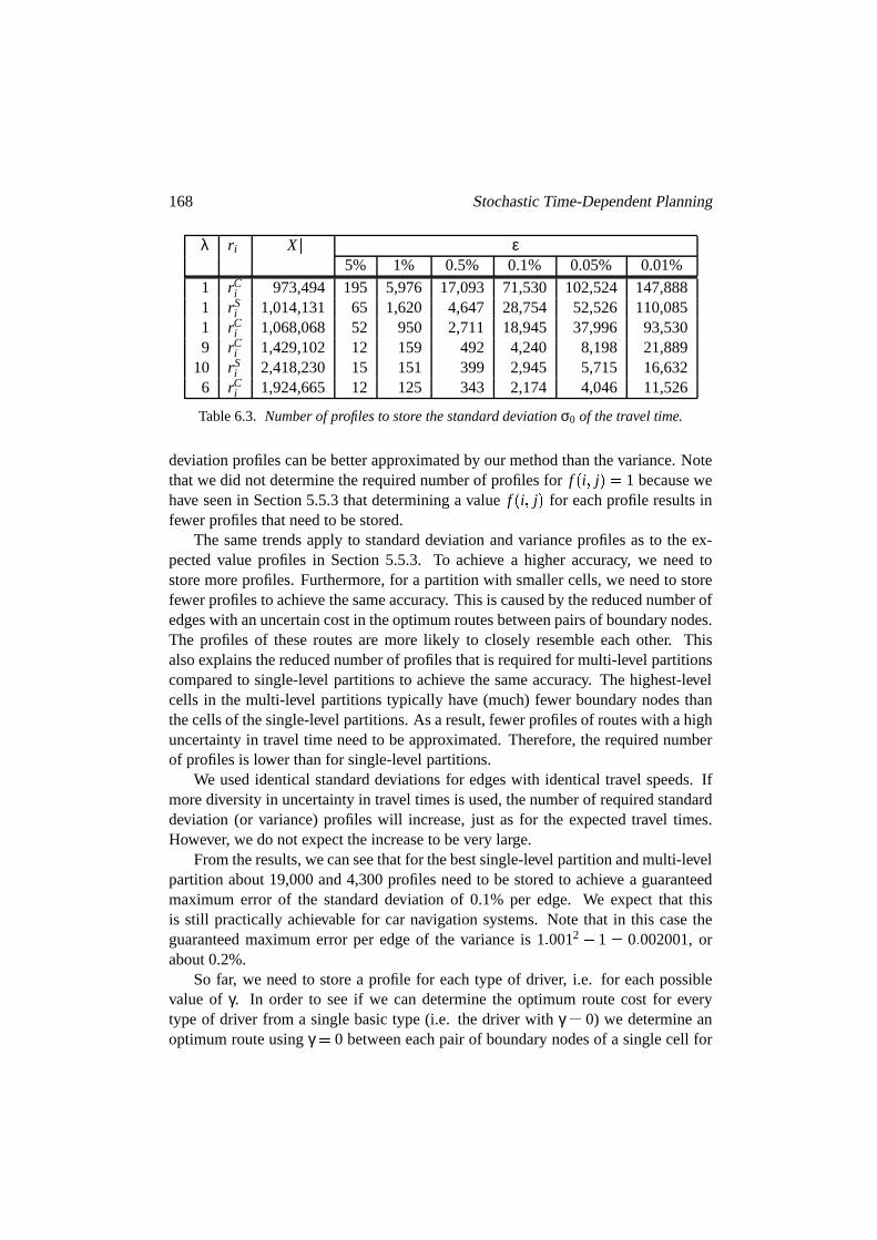
168 StochasticTime-DependentPlanning
λ r i ØX Ø ε5% 1% 0.5% 0.1% 0.05% 0.01%
1 rCi 973,494 195 5,976 17,093 71,530 102,524 147,888
1 rSi 1,014,131 65 1,620 4,647 28,754 52,526 110,085
1 rCi 1,068,068 52 950 2,711 18,945 37,996 93,530
9 rCi 1,429,102 12 159 492 4,240 8,198 21,889
10 rSi 2,418,230 15 151 399 2,945 5,715 16,632
6 rCi 1,924,665 12 125 343 2,174 4,046 11,526
Table6.3. Numberof profilesto store thestandard deviation σ0 of thetraveltime.
deviation profilescanbebetterapproximatedby ourmethodthanthevariance.Notethatwe did not determinetherequirednumberof profilesfor f Ê i Í j Ì É 1 becausewehave seenin Section5.5.3thatdetermininga value f Ê i Í j Ì for eachprofile resultsinfewer profilesthatneedto bestored.
The sametrendsapply to standarddeviation andvarianceprofilesasto the ex-pectedvalue profiles in Section5.5.3. To achieve a higher accuracy, we needtostoremoreprofiles.Furthermore,for a partitionwith smallercells,we needto storefewerprofilesto achieve thesameaccuracy. This is causedby thereducednumberofedgeswith anuncertaincostin theoptimumroutesbetweenpairsof boundarynodes.The profiles of theseroutesare more likely to closely resembleeachother. Thisalsoexplainsthereducednumberof profilesthatis requiredfor multi-level partitionscomparedto single-level partitionsto achieve thesameaccuracy. Thehighest-levelcells in the multi-level partitionstypically have (much)fewer boundarynodesthanthecellsof thesingle-level partitions.As aresult,fewerprofilesof routeswith ahighuncertaintyin travel time needto beapproximated.Therefore,therequirednumberof profilesis lower thanfor single-level partitions.
We usedidenticalstandarddeviationsfor edgeswith identicaltravel speeds.Ifmorediversityin uncertaintyin travel timesis used,thenumberof requiredstandarddeviation (or variance)profileswill increase,just as for the expectedtravel times.However, we do notexpecttheincreaseto bevery large.
Fromtheresults,wecanseethatfor thebestsingle-level partitionandmulti-levelpartition about19,000and4,300profilesneedto be storedto achieve a guaranteedmaximumerror of the standarddeviation of 0.1% per edge. We expect that thisis still practicallyachievable for car navigation systems.Note that in this casetheguaranteedmaximumerror per edgeof the varianceis 1 Î 0012 Ë 1 É 0 Î 002001,orabout0.2%.
So far, we needto storea profile for eachtype of driver, i.e. for eachpossiblevalue of γ. In order to seeif we candeterminethe optimum route cost for everytype of driver from a singlebasictype (i.e. thedriver with γ É 0) we determineanoptimumrouteusingγ É 0 betweeneachpair of boundarynodesof a singlecell for

6.5 Combinationwith Partitions 169
departuretimes0 Í 900Í Î Î Î�Í 86Í 400.Wealsodeterminethenumberof time-dependentedgesLt Ê pÌ in eachfoundroutep for eachdeparturetime andthevalueof µγ andσγ
for γ É 1 Í 2 Í 3. Giventhesevalueswedetermineyi É ln Ê µγ ì µ0
γσ0Ì , andxi É ln Ê Lt Ê pÌ Ì for
eachrouteandeachdeparturetime. This leadsto acollection Ê y1 Í x1 Ì�Í Î Î Î�Í Ê y! Í x! Ì forγ É 1 Í 2 Í 3.
As explained in Section6.5.2, the value of µγ can be approximatedby µ0 âγ � Ê Lt Ê pÌ Ì ζσ0. So we would like to determinehow accuratethe valuesof µγ aredescribedby µ0 â γ � Ê Lt Ê pÌ Ì ζσ0, or equivalently how accuratethe valuesof yi Éln Ê µγ ì µ0
γσ0Ì aredescribedby ζxi É ζ ln Ê Lt Ê pÌ Ì . Note that becauselimxs 0 ln Ê xÌ É�Ë ∞
andbecausefor routeswith no time-dependentedges(Lt Ê pÌ É 0) we have µγ É µ0
andσ0 É 0, we only needto computeyi andxi for thoserouteswith Lt Ê pÌ � 0 orequivalently for routeswith µγ ñÉ µ0. In orderto determinethevalueof ζ suchthatthevaluesof yi arebestdescribedby xi , we uselinearregression.
We have a collectiony1 Í Î Î Î�Í y! anda collectionx1 Í Î Î Î�Í x! , andwe determinethevalueof ζ suchthaty1 Í Î Î Î�Í y! is bestapproximatedby ζx1 Í Î Î Î�Í ζx! . Usingtheordinaryleastsquaresmethod[Montgomery, Peck& Vining, 2001],this leadsto
ζ É ∑ !j ß 1 y jx j
∑ !j ß 1x2
j
Íand
R2 É ∑ !j ß 1 Ê ζx j Ë 1! ∑ !
i ß 1yi Ì 2∑ !
j ß 1 Ê y j Ë 1! ∑!i ß 1 yi Ì 2 Î
Herethe regressioncoefficient R2 Ùt� 0 Í 1� denotesthequality of theapproximation.Note thatR2 É 1 denotesa perfectapproximation,soyi É ζxi for every i É 1 Í Î Î Î�Í � ,andR2 É 0 denotesthatζxi givesno informationat all aboutthevalueof yi .
We alsodetermineyÜi É ln Ê µγ ì µ0
σ0Ì for eachrouteandeachdeparturetime for γ É
1 Í 2 Í 3. This leadsto thecollectionyÜ1 Í Î Î Î�Í yÜ! . Subsequently, we determinevaluesζ Ü0andζ Ü1 suchthat Ê yÜ1 Í Î Î Î�Í yÜ! Ì is bestapproximatedby Ê ζ Ü0 â ζ Ü1x1 Í Î Î Î�Í ζ Ü0 â ζ Ü1x! Ì . Usingtheordinaryleastsquaresmethodthis leadsto
ζ Ü1 É �∑ !
j ß 1yÜ jx j Ë ∑!i ß 1xi ∑
!i ß 1 yÜi�
∑ !j ß 1 x2
j Ë|Ê ∑ !j ß 1x j Ì 2 Í
ζ Ü0 É 1� !∑j ß 1
yÜ j Ë ζ Ü11� !∑i ß 1
xi Íand Ê RÜ Ì 2 É ∑ !
i ß 1 Ê Ê � ∑ !i ß 1 xiyÜi Ë ∑!
i ß 1 xi ∑!i ß 1yÜi Ì 2Ê � ∑ !
i ß 1 x2i Ë|Ê ∑ !
i ß 1xi Ì 2 Ì Ê � ∑ !i ß 1 Ê yÜi Ì 2 Ë Ê ∑ !
i ß 1yÜi Ì 2 Ì ÎWe have computedthevaluesof ζ, eζ u0, ζ Ü2 andR2, Ê RÜ Ì 2 for differentpartitions,andfor different valuesof γ, by determiningthe valueof yi , yÜi andxi for eachpair of

170 StochasticTime-DependentPlanning
boundarynodesof a cell andfor every departuretime t with t É 0 Í 900Í Î Î Î�Í 86Í 400.Theresultscanbefoundin Table6.4.
λ r i γ ζ R2 eζ u0 ζ Ü1 Ê RÜ Ì 21 rC
i 1 0.384222 0.751844 0.880170 0.424964 0.9183301 rC
i 2 0.384131 0.751866 1.760861 0.424778 0.9179961 rC
i 3 0.384027 0.751448 2.642566 0.424520 0.9168781 rS
i 1 0.380395 0.765625 0.913523 0.413507 0.9034851 rS
i 2 0.380356 0.765894 1.826628 0.413551 0.9041751 rS
i 3 0.380308 0.765917 2.740608 0.413415 0.9038381 rC
i 1 0.375157 0.780584 0.931246 0.402833 0.8989821 rC
i 2 0.375129 0.781077 1.861843 0.402940 0.9001521 rC
i 3 0.375092 0.781334 2.793418 0.402812 0.9000619 rC
i 1 0.375819 0.817700 0.964804 0.394341 0.8988689 rC
i 2 0.375838 0.822487 1.929665 0.394345 0.9040579 rC
i 3 0.375834 0.824251 2.895213 0.394214 0.90542910 rS
i 1 0.347554 0.765900 0.992562 0.353245 0.79103810 rS
i 2 0.347688 0.783482 1.984237 0.353723 0.81074210 rS
i 3 0.347705 0.790632 2.977615 0.353417 0.8166656 rC
i 1 0.383486 0.890168 0.979860 0.392968 0.9340426 rC
i 2 0.383533 0.897175 1.959637 0.393034 0.9414796 rC
i 3 0.383532 0.900212 2.940574 0.392856 0.943840
Table6.4. Relationµγ Ï µ0 . γ Ð Lt Ð pÒ:Ò ζσ0 andµγ Ï µ0 . eζ u0 Ð Lt Ð pÒµÒ ζ u1σ0.
As we canseefrom Table6.4 we find ζ � 0 Î 5 (andalsoζ Ü1 � 0 Î 5) asexpected.Inparticular, weseethatζ � ζ Ü1 andeζ u1 � γ. Furthermore,wecanseethattheregressioncoefficient Ê RÜ Ì 2 is largerthanR2. Thiscanbeexplainedby thefactthatdeterminingtwo parametersto approximatethevaluesyi leadsto betterresultsthandeterminingonly a singlevalue. We canseethat µ0 â γ Ê Lt Ê pÌ Ì 0 : 375σ0 seemsto reasonablyap-proximatethe value of µγ for different partitions,where0 Î 375 is the averageof ζin column4. However, thequality of approximatingµγ by µ0 â eζ u0 Ê Lt Ê pÌ Ì 0: 397σ0 isclearlybetterjudgingfrom R2 and Ê RÜ Ì 2, where0 Î 397is theaverageof ζ Ü1 in column7. Note that for both relationswe have µγ É µ0 for routeswith no time-dependentedges(i.e. routeswith Lt Ê pÌ É 0) asshouldbe the case. We canalsoseethat wecanapproximateeζ u0 by γeζ u2 with eζ u2 É 0 Î 944for all testedpartitions,where0 Î 944is
theaverageof eζ u0γ which canbecomputedusingthedatain column6. This leadsto
µγ É µ0 â 0 Î 944γ Ê Lt Ê pÌ Ì 0: 397σ0. Sowecanconcludethatwe areableto approximateµγ reasonablycloseby using
µγ É µ0 â γeζ u2 Ê Lt Ê pÌ Ì ζ u1σ0 Í

6.5 Combinationwith Partitions 171
whereζ Ü1 andeζ u2 areindependentof γ. We candeterminethevalueof ζ Ü1 for a par-ticular partitionby themethoddescribedabove. Thevalueof eζ u2 canbesetequalto
the averageof eζ u0γ for differentvaluesof γ, or to eζ u0 for γ É 1. As a result,we can
plan stochastictime-dependentroutesfor different typesof drivers (with differentpreferredγ andβ) usingpartitionedroadgraphsby storingonly theexpectationandvarianceof theoptimumtravel timeandcostfor γ É 0 betweeneachpairof boundarynodesof asinglecell. Thequalityof thisapproximationis reasonableascanbeseenfrom Table6.4.
We can also approximatethe value of σγ by σ0 as indicatedin Section6.5.2.We canagainuselinear regressionto determinea relationbetweenσγ andσ0. Foreachfound routeand for eachdeparturetime we computeyi É σγ, γ É 1 Í 2 Í 3 andxi É σ0. Usingthedefinitionsof ζ, andR2 andζ Ü0, ζ Ü1, Ê RÜ Ì 2 this leadsto theresultsinTable6.5.
λ r i γ ζ R2 ζ Ü0 ζ Ü1 Ê RÜ Ì 21 rC
i 1 1.001203 0.998743 -0.015166 1.001621 0.9995771 rC
i 2 1.002514 0.996804 -0.029633 1.003333 0.9984331 rC
i 3 1.003861 0.994348 -0.042689 1.005045 0.9966921 rS
i 1 1.000631 0.999399 -0.005697 1.000830 0.9997951 rS
i 2 1.001307 0.998451 -0.011253 1.001700 0.9992341 rS
i 3 1.002000 0.997227 -0.016378 1.002573 0.9983661 rC
i 1 1.000541 0.999525 -0.004187 1.000698 0.9998391 rC
i 2 1.001100 0.998777 -0.008197 1.001408 0.9993921 rC
i 3 1.001666 0.997806 -0.011886 1.002113 0.9986979 rC
i 1 1.000269 0.999876 -0.000726 1.000326 0.9999899 rC
i 2 1.000508 0.999745 -0.001359 1.000614 0.9999589 rC
i 3 1.000720 0.999606 -0.001907 1.000869 0.99990410 rS
i 1 1.000217 0.999916 -0.000501 1.000254 0.99999010 rS
i 2 1.000421 0.999817 -0.000970 1.000493 0.99996010 rS
i 3 1.000616 0.999704 -0.001414 1.000720 0.9999136 rC
i 1 1.000259 0.999894 -0.000582 1.000306 0.9999896 rC
i 2 1.000488 0.999778 -0.001090 1.000576 0.9999556 rC
i 3 1.000684 0.999652 -0.001519 1.000808 0.999898
Table6.5. Relationσγ Ï ζσ0 andσγ Ï ζ v0 . ζ v1σ0.
FromTable6.5we seeagainthatusingtwo parametersto approximatethevalueofσγ is betterthanusingonly a singlevaluesinceR2 � Ê RÜ Ì 2. However thedifferenceis muchsmallerthanin Table6.4. Furthermore,we seethat thecomputedvalueofζ Ü0 is negative. Becausethestandarddeviation of a routecannever benegative, andthedifferencebetweenR2 and Ê RÜ Ì 2 is very small,we prefertherelationσγ É ζσ0 toσγ É ζ Ü0 â ζ Ü1σ0. We canseethatζ � 1 andalsoζ Ü0 � 0, ζ Ü1 � 1 soapproximatingσγ

172 StochasticTime-DependentPlanning
by σ0 is reasonable.Consideringthevaluesof ζ weseethatwecanapproximateζ by1 â γζ1 with ζ1 É 0 Î 00125for asingle-level partitionwith r i É bi Ê bi Ë 1Ì for example,where0 Î 00125is the averageof ζ
γ for single-level partitionswith rCi . Similarly, ζ Ü1
canbeapproximatedby 1 â γζ Ü2 andζ Ü0 by γζ Ü3 with ζ Ü2 É 0 Î 00166andζ Ü3 É Ë 0 Î 015forsingle-level partitionswith r i É bi Ê bi Ë 1Ì for example,where0 Î 00166and Ë 0 Î 015
are the averagesof ζ u1 ì 1γ and ζ u0
γ respectively. As mentionedbefore,we prefer therelationσγ É ζσ0. Sofor a particularpartition,we candetermineavalueζ usingthe
methoddescribedabove. Subsequentlywe computeζ1 by takingtheaverageof ζ ì 1γ
for differentvaluesof γ or by settingζ1 É ζ for γ É 1. Thenwe canapproximateσγby
σγ ÉwÊ 1 â γζ1 Ì σ0 ÎAs canbeseenfrom thevaluesof R2 in Table6.5thisapproximationis quitegood.
6.6 Conclusion
In this chapterwe have discussedtheplanningof stochastictime-dependentroutes.First of all, we discussedunderwhich conditionswe can plan optimum stochas-tic time-dependentroutesby usinga modifiedversionof a standardrouteplanningalgorithmsuchastheAÚ -algorithm.Assumingtheseconditionsaresatisfied,wepre-sentedarouteplanningalgorithm,theSÚ -algorithmthatcanbeusedto planoptimumstochastictime-dependentroutes. Planningoptimum stochasticroutes,requiresadefinition of theoptimality (or cost)of a route. We formulateda costandoptimal-ity conditionthatcanbalanceuncertainty(or equivalently thestandarddeviation) intravel timeagainsttheexpectedtravel time. Thiscanbeusedto representtheattitudeof mostdrivers towardsuncertaintyin their travel times. Becausea car navigationsystemhasto plan routesfast,andbecausethedeterminationof theexactexpectedtravel time of a routeandits varianceis very complicated,we usedapproximationsto determinethevarianceandexpectedvalueof thetravel time of a route. It wouldbe very interestingto determinethe expectedtravel time and its varianceexactlythough. Ideally, we would like to be ableto determinethesevaluesfast. Further-more,we would like to requireonly theexpectedtravel time andvarianceof a routeÓe1 Í Î Î Î�Í e! Ô togetherwith dataonedgee! ë 1 to determinetheexpectedtravel timeand
varianceof routeÓe1 Í Î Î Î�Í e! ë 1 Ô exactly.
Usingreal-world dataonuncertaintyin travel times,weevaluatedtheusefulnessof stochastictime-dependentrouteplanningby planning2,000fastestroutesthroughtheNetherlands.Fromtheresults,weconcludedthatstochastictime-dependentplan-ning canbe very useful,but only if thedriver desiresa high level of certaintycon-cerninghis (latestpossible)arrival time.
We useda single expectedtravel time profile for all motor- and highways inthe Netherlands.We determinedthe standarddeviation of the travel time by divid-

6.6 Conclusion 173
ing thedifferencebetweenthemaximumtime-independenttravel time andthetime-dependenttravel timeby afixedfactorς thatis thesamefor all motor- andhighways.Justas for deterministictime-dependentroute planning,we canalso usedifferentstochasticprofilesfor differentmotorways. This canbedoneby computinga valueς for every motorway. Alternatively, we canalsousevarianceor standarddeviationprofilesjust asfor themeantravel speed.In orderto usedifferentstochasticprofilesfor eachmotorway, we alsoneedto determinewhich edgesarepart of a particularmotorway. Theproblemof determiningtheexpectedtravel time of a singleedgeissimilar to theproblemfor deterministictime-dependenttravel speeds.For stochastictime-dependentplanning,we alsoneedto determinethevariance(or standarddevia-tion) of thetravel timeof asingleedgegiventhevarianceof thetravel timeof arouteconsistingof multiple edges.Like theexpectedtravel time, thevarianceof thetraveltime is mostlikely to belargerneara junctionthatcausesmostcongestion.Notethatalsolessimportantroadsaresubjectto uncertaintyin their travel times,soa modelcould alsobe developedfor the uncertaintyin travel timeson roadsfor which theuncertaintyin travel timescannotbedeterminedfrom reportedtravel times.
Wealsoinvestigatedthepossibilitiesto combinestochastictime-dependentplan-ning with partitions. In order to plan optimumstochasticrouteswith a partitionedroadgraph,weneedto storealot of informationonroutesbetweenboundarynodesofsinglecells. If optimality of stochasticroutesis not requiredandhigh-qualityroutesaresatisfactory, which is usually the casein stochastictime-dependentrouteplan-ning, thentheplanningof stochastictime-dependentroutesin partitionedroadgraphis possiblewith only moderatestoragerequirements.We presentedan approachtostoretherequireddataonstochasticroutesby creatingprofilesof theexpectedtraveltime andstandarddeviation. The requirednumberof profilescanbe substantiallyreducedby approximatingtheseprofilesusingtheX-MATCH algorithmpresentedinChapter5. Like for deterministictime-dependenttravel times,we needa differentalgorithmto determinetheminimumnumberof profilesneededto storetheexpectedtravel times. This methodcanalsobe usedto determinethe minimum numberofprofilesneededto storethestandarddeviation of travel timesfor a pre-specifiedac-curacy.
Finally, we have seenthattheexpectationandvarianceof thecostof aparticularroutefor differentattitudesof thedrivercanbeapproximatedreasonablywell by stor-ing only thecostsaccordingto onebasicattitude.As aresult,high-qualitystochastictime-dependentroutescanbe plannedfastfor all kinds of differenttypesof driversin partitionedroadgraphsrequiringonly limited storagespace.Alternative methodsto determinetheroutecostfor differenttypesof driversbasedon onebasictypecanalsobedeveloped.Furthermore,anexpressionof thequalityof thedeterminedrouteswouldbeinteresting.

174 StochasticTime-DependentPlanning

7Comparisonwith ProductRoutePlanners
In the previous chapters,we have describedrouteplanningalgorithmsthat canbeusedto plan optimum routesin time-independent,time-dependentand stochastictime-dependentroadgraphs.Of course,currentlycarnavigationsystemsalreadyusea routeplanningalgorithmto determinea routefrom a startnodes to a destinationnoded. Section7.1 briefly discussesthe route planningalgorithm that is imple-mentedin productversionsof car navigation systems.After describingthis routeplanningalgorithm,we comparetheaverageperformanceof this algorithmwith ourCÚ -algorithmfor planningtime-independentroutesin Section7.2, andwe will seethat theCÚ -algorithmplansoptimumroutesfasteron averagethancurrentproductroute plannersplan non-optimumroutes. Section7.3 discussessomeexceptionalcasesin whichouralgorithmperformsmuchbetterthantheusedproductrouteplan-ner. Theadvantagesanddisadvantagesof ourapproacharediscussedin Sections7.4and7.5 respectively. In Section7.6,we discusshow additionalrouteplanningfunc-tionality offeredin car navigation systems,for exampleplanningalternative routes,canbe implementedusingpartitionedroadgraphs.Section7.7 presentsthe conclu-sions.
7.1 Standard RoutePlanner Algorithms
The routeplanningalgorithm implementedin (most) car navigation systemsis anapproximationalgorithmthatis basedon theAw -algorithm. It thusis not guaranteed
175

176 Comparisonwith ProductRoutePlanners
thatanoptimumroutefrom astartnodes to adestinationnoded is planned.Wewillcall thisalgorithmtheRP-algorithm.
TheRP-algorithmis basedon a division of theroadnetwork into moreandlessimportantroads. As was alreadyindicatedin Section5.4, every road segmentofthe roadnetwork, or equivalently, every edgein the roadgraph,hasbeenassignedacertainroadclass.This roadclasscanbeusedto indicatethe importanceof a road:thehighertheroadclassnumberthelessimportanttheroad.For example,edgeswithroadclass0 aremainlymotorwaysandedgeswith roadclass1 aremainlyhighways.
The RP-algorithmbasicallyevaluatesedgesof all roadclassesnearthe car andthe destination,andthe larger the distanceto the car or destination,the higher theimportanceof anedgeneedsto befor thealgorithmto evaluatethatedge.Notethatthisbasicallycorrespondsto thewayhumansplana route.
Specifically, the roadgraphis divided into a numberof levels. The roadclassof an edgecan for examplebe usedto divide the road network into levels. Themost detailedlevel is called the detailed network (DT), and it containsall edgesfor exampleof all roadclasses.Also a numberof higher levels arecreated,calledthe High-Level networks (HL). Thesehigh-level networks containfor examplealledgesof at leasta certainroadclass.For example,a HL network canbecreatedthatconsistsof all edgesof roadclass3, 2, 1 and0. Wecall thisnetwork HL3. Similarly,theHL network consistingof all edgeswith roadclass0 is calledHL0. So,for aroadnetwork with 7 possibleroadclasses(0-6)wecancreatefor example6 possiblehighlevel networks (HL0-HL5) anda detailednetwork DT. Note that the network HL6would correspondto thenetwork DT. Thecreationof theDT network anda numberof HL networksis donebeforehand,andthesenetworksarestoredontheCD or DVDcontainingthemap.Usually, atmostthreeHL networksareactuallycreated.
Whena routeneedsto be planned,the RP-algorithmfirst determinesareasforexamplearoundthecaranddestinationposition.Theseareasindicatein which areathealgorithmshouldusewhich network. If thecaranddestinationarelocatedveryclosetogetherthealgorithmgenerallyonly usestheDT network. However, for acaranddestinationpositionlocatedfarapart,theDT network is generallyonly usedverycloseto thecaranddestinationposition.
Specifically, areasarecreatedfor every network exceptfor theleastdetailednet-work. So, if for examplea DT network and threeHL networks arestoredon theCD or DVD, thenfor exampletwo areas(onesurroundingthe destinationandonesurroundingthe car position)arecreatedfor threeof thesenetworks, in this case6areas.Undercertainconditionsmultiple areasfor a singlenetwork canbecombinedinto onearea,seefor exampleFigure7.1.
Thesearchgraphof theRP-algorithmconsistsof all edgesof anetwork containedin theareasfor thatnetwork. For example,if only a DT, a HL2 anda HL0 networkexist, then the searchgraphconsistsof all edgescontainedin the areasof the DT

7.2 AveragePerformanceof theCw - andRP-Algorithm 177
DT
HL2
DT
HL2
HL1
HL0
s d
Figure7.1. Exampleof areasusedby theRP-algorithm.
network, all edgesin the HL2 network that arecontainedin the areasof the HL2network, and all edgesin the HL0 network locatedoutsidethe areasof the HL2network.
The RP-algorithm then usesa modified Aw -algorithm to plan a route on thissearchgraph.The estimatedcost from a location to the destinationusuallyoveres-timatestheactualcostto increasetheplanningspeed.After aninitial routehasbeenfound the driver receivesadvice. We call this routean initial route. Subsequently,theRP-algorithmfinishesthecurrentroute,for exampleby trying to improve it. Theresultingrouteis calledafinal route.
7.2 AveragePerformanceof the Cx - and RP-Algorithm
This sectioncomparesthe average-caseperformanceof the RP-algorithm1 andtheCw -algorithm.In orderto comparetheaverageperformanceof thesetwo routeplan-ning algorithms,we plan the fastestandshortestroutesbetweenall 2,000startanddestinationnodesroutesfrom our routebatch,seeTable4.3,usingthemaximumal-lowed travel speedsthat dependon the roadclass. We useboth algorithmsto plantheseroutes,andwecomparethenumberof evaluatededgesandtheroutelengthsanddriving times. In orderto achieve a fair comparison,we needto usethesamecostsfor eachedge,or similarly, thesamelengthsanddriving speeds.Note that theRP-algorithmsweusedfor comparisoncanusetwo differentspeeds,adriving speedanda planningspeedwhich incorporatesalsootherfactorsbesidespuredriving speeds.Thedriving speedsasusedin Chapter4arenotexactlythesameastheuseddriving or
1We usedthe VDO Daytonrouteplanningalgorithmdevelopedby SiemensVDO Automotive inEindhovenasbasisfor our comparisons.

178 Comparisonwith ProductRoutePlanners
planningspeedsby theRP-algorithm.Becausethespeedsusedby theRP-algorithmarelesseasyto adapt,we modifiedthespeedsusedby theCw -algorithm.Therefore,the resultsof theCw -algorithmusingthesemodifiedspeedsaresomewhat differentfrom theresultsin Chapter4. Notethatfor thedriver theresultsusingdriving speedsseemmost important. However, the RP-algorithmis specificallytunedto performwell usingplanningspeeds.Furthermore,we modifiedthe RP-algorithmsuchthatit usesonly the lengthof edgesto determineshortestroutes.We usethemulti-levelpartition generatedwith r i y bi z bi { 1| as input for our Cw -algorithm,becausewehave seenin Chapters3 and4 that this partition leadsto the leastnumberof edgesevaluatedby therouteplanningalgorithm.
The datausedto createour partitionshasa different format than the standarddatabasesusedby thecurrentrouteplannerof SiemensVDO Automotivebut they arebothbasedonCENGDF3.0data(GeographicDataFiles),suppliedby NavTeq.GDFis a European(CEN) standard,that is usedto describeandtransferroadnetworksand road relateddata. As a result, the roadgraphbasedon the standarddatabaseof SiemensVDO Automotive is slightly different from our roadgraph.Sometimesa singleedgein the roadgraphusedfor partitioning is representedby two or moreedgesin the roadgraphusedby theRP-algorithm. However, theseadditionaledgesarecreatedso that partsof the roadgraphcanbe readfrom a CD or DVD insteadof just theentireroadgraph.Whena partitionis used,theseadditionaledgesarenotneededbecausetheroadgraphis alreadypartitionedinto cellswhichcanbereadfromtheCD or DVD separately.
The resultsof the average-caseperformanceof the RP-algorithm and the Cw -algorithmcanbefoundin Tables7.1and7.2.Theresultsfor initial routesaredenotedby (I) and thosefor final routesby (F). Columns2 and 5 presentthe numberofevaluatededges,columns3 and6 presentthedriving time in seconds,andcolumns4and 7 presentthe route length in meters. In the road network several nodesexistwith identicalcoordinates,for exampleat cloverleafjunctions.If thetwo algorithmsselectdifferentnodes,theresultingroutesarequitedifferent.Theserouteshavebeenremovedfrom thecomparisonbetweenindividual routesin row 4 and5 of Tables7.1and7.2.
The RP-algorithmrequireson averagemoreedgeevaluationsto plan the 2,000routesfrom our routebatchthantheCw -algorithm. As explainedin Section7.1 theRP-algorithmis an approximationalgorithmanddoesnot alwaysfind an optimumrouteunlike theCw -algorithm.Wecanseefrom theresults,thateventhoughtheCw -algorithmsneedsto evaluatefewer edgesthanthe RP-algorithm,theCw -algorithmplansoptimum routes,while the routesplannedby the RP-algorithm may have acost that is above optimum. Specifically, using driving (or planning)speeds,thetime anddistancearemorethan8 (or 4.5) minutesand7 (or 6.5) kilometersaboveoptimumfor initial fastestandshortestroutesrespectively. After trying to improve

7.2 AveragePerformanceof theCw - andRP-Algorithm 179
Algorithm Fastestroute ShortestrouteEval. Time Length Eval. Time LengthEdges (s) (m) Edges (s) (m)
Cw 1,548 4,143 97,647 1,333 5,670 87,331RP(I) 1,619 4,588 102,936 2,285 5,021 94,518RP(F) - 4,468 100,271 - 5,037 92,450RP { Cw (I) 112 494 5,098 951 -631 7,325RP { Cw (F) - 373 2,553 - -658 5,577RP} C~
C~ (I) 1.61 0.16 0.10 3.00 -0.01 0.13RP} C~
C~ (F) - 0.11 0.04 - -0.03 0.06
Table7.1. ComparisonaverageresultsRPandC� with driving speeds.
Algorithm Fastestroute ShortestrouteEval. Time Length Eval. Time LengthEdges (s) (m) Edges (s) (m)
Cw 1,628 4,089 100,612 1,333 8,221 87,331RP(I) 1,652 4,350 103,650 2,158 5,153 94,262RP(F) - 4,225 101,432 - 5,236 92,234RP { Cw (I) 19 267 2,785 826 -3,061 6,993RP { Cw (F) - 150 704 - -2,977 4,962RP} C~
C~ (I) 1.33 0.08 0.07 2.43 -0.29 0.12RP} C~
C~ (F) - 0.04 0.01 - -0.29 0.06
Table7.2. ComparisonaverageresultsRPandC� with planningspeeds.
thefoundroutes,thefinal routesarestill morethan6 (or 2.5)minutesand5 (or 4.5)kilometersabove optimumfor fastestandshortestroutesrespectively usingdriving(or planning)speeds.Thefourth andfifth row comparetheresultsfor theindividualplannedroutesby theCw - andtheRP-algorithm. Therefore,thedifferencebetweenthefirst two rows,andthefirst andthird row in Tables7.1and7.2arenotequalto theresultsin thefourthandfifth row of Tables7.1and7.2respectively. Also therelativedifferenceshave beendeterminedby takingtheaverageof therelative differenceforeachroute. Note thatwe did not includethenumberof edgesevaluatedto improvetheinitial routesbecausethis improvementis donewhile thedriver alreadyreceivesguidance.Thespeedof this mechanismis thusnot very important.We canalsoseethat theRP-algorithmis muchfasterthanthestandardAw -algorithmfrom Table4.4andTable4.5. Although the resultsin Tables4.4 and4.5 weregeneratedusing aroadgraphwith slightly differentedgecosts,the numberof edgesevaluatedby theAw -algorithmusingtheroadgraphfrom thissectionwill becomparable.

180 Comparisonwith ProductRoutePlanners
7.3 Exceptional Casesof the RP-Algorithm
Section7.2 discussedthe average-caseperformanceof theCw -algorithmcomparedto the RP-algorithm. Unlike theCw -algorithm,the RP-algorithmis not guaranteedto plan optimumroutes. This sectionpresentssomeworst-caseresults. Again thedriving time of an edgedependson the maximumallowed driving speedwhich, inturn, dependson theedge’s roadclass.Theresultsof theworst-casecomparisonoftheRP-algorithmandtheCw -algorithmcanbe found in Tables7.3 and7.4. Resultsfor initial routesaredenotedby (I) andthosefor final routesby (F). Columns2 and5presentthe numberof evaluatededges,columns3 and 6 presentthe driving timein seconds,andcolumns4 and 7 presentthe route length in meters. Like for theaverage-caseresultsin Tables7.1and7.2,routesfor which thetwo algorithmsselectdifferentstartor destinationnodeshave beenremovedfrom thecomparisonbetweenindividual routesin row 4 and5 of Tables7.3and7.4. Note thatTables7.3and7.4give themaximumnumberof evaluatededges,themaximumroutetravel time, andthemaximumroutelengthfor bothfastestandshortestroutes.Theroutesfor whichthesemaximaareattainedarenotnecessarilythesame.
Algorithm Fastestroute ShortestrouteEval. Time Length Eval. Time LengthEdges (s) (m) Edges (s) (m)
Cw 6,440 32,302 418,528 6,159 35,108 386,120RP(I) 15,888 33,867 425,856 443,390 42,551 402,726RP(F) - 33,869 418,816 - 36,051 399,872RP { Cw (I) 15,508 4,011 134,455 443,094 16,098 198,266RP { Cw (F) - 2,639 63,371 - 2,307 36,779RP} C~
C~ (I) 40.81 29.77 53.68 1,496.94 29.77 53.68RP} C~
C~ (F) - 0.77 0.90 - 1.27 0.68
Table7.3. Comparisonworst-caseresultsRPandC� with driving speeds.
Fromtheresultsin Tables7.3and7.4,wecanseethatthemaximumnumberof edgesevaluatedby theCw -algorithmis muchsmallerthanfor the RP-algorithm. Specifi-cally, a fastestrouteexists for which theRP-algorithmneedsto evaluate15,888(or18,297)edgesto find aninitial routeusingdriving (or planning)speeds,while theCw -algorithmdoesnotneedmorethan380(or 388)edgeevaluationsfor thesameroute.In casea shortestrouteneedsto beplannedthesituationis evenworse.Thereexistsan initial routefor which the RP-algorithmneedsto evaluate403,390(or 100,463)edges,while theCw -algorithmonly needsto evaluate296(or 296)edgesto find theoptimumrouteusingdriving (or planning)speeds.For planningfastestroutestheCw -algorithmrequires(for these2,000startanddestinationnodes)a maximumofabout6,400edgeevaluations,which is about4 timestheaveragenumberof evalu-

7.3 ExceptionalCasesof theRP-Algorithm 181
Algorithm Fastestroute ShortestrouteEval. Time Length Eval. Time LengthEdges (s) (m) Edges (s) (m)
Cw 6,322 17,719 432,962 6,159 35,714 386,120RP(I) 18,297 18,930 422,916 100,463 23,397 403,486RP(F) - 18,726 419,984 - 23,431 402,656RP { Cw (I) 17,909 2,835 134,522 100,167 7,460 67,553RP { Cw (F) - 2,347 47,107 - 2,604 36,779RP} C~
C~ (I) 46.16 16.17 53.68 338.40 16.17 53.68RP} C~
C~ (F) - 0.63 0.77 - 0.71 0.67
Table7.4. Comparisonworst-caseresultsRPandC� with planningspeeds.
atededges(which is about1,600). For shortestroutesplannedby theCw -algorithmthemaximumnumberof evaluatededgesis about6,150.This is lessthan5 timestheaverage(of about1,300). The RP-algorithmrequiresfor these2,000fastestroutesa maximumof about16,900edgeevaluations,which is about10 times the aver-agenumberof evaluatededges(which is about1,600). For shortestroutesthe RP-algorithmneedsto evaluateamaximumof about440,000edges,which is evenmorethan45 timesthe averagenumberof evaluatededges(which is about2,200). Thelarge differencebetweenthe resultsfor planningfastestandshortestroutesby theRP-algorithmis causedby the fact that a differentdefinition of the searchgraphisusedfor planningfastestandshortestroutes. Note that the theoreticalupperboundon the maximumrequirednumberof edgesevaluatedby theCw -algorithm canbededucedfrom theconstructedpartitions.Specifically, themaximumnumberof eval-uatededgesis equalto the maximumnumberof edgesin the searchgraph.For theRP-algorithmanupperboundon thenumberof evaluatededgesdoesnotexist.
In worst-case(of the 2,000 routes found by the RP-algorithm using drivingspeeds)theinitial routepresentedby theRP-algorithmcanhave a time of morethan1 houranda lengthof almost200kilometersabove theoptimumtime andlengthofthefastestandshortestrouterespectively. For final routesthis is still 44 minutesandmorethan36 kilometersabove theoptimumtimeandlengthof thefastestandshort-estrouterespectively, seerow 4 and5 of Table7.3. Furthermore,theRP-algorithmis not ableto find 6 fastestand4 shortestinitial routes,and8 fastestand4 shortestfinal routes,outof the2,000startanddestinationnodes.Wecanalsoseethatthedif-ferencebetweenthefirst two rows andbetweenthefirst andthird row in Tables7.3and7.4 arenot equalto theresultsin thefourth andfifth row of Tables7.3 and7.4.This is becausethefourthandfifth row in Tables7.3and7.4comparetheresultsfortheindividual routesplannedby theCw - andtheRP-algorithm.Notethat theresultsfor lengthandtime in row RP} C~
C~ (I) in Tables7.3and7.4aresomewhatmisleading.

182 Comparisonwith ProductRoutePlanners
They arecausedby a routethatis only 25 meterslong. If this routeis not takenintoaccountthenthevaluesdecreaseto atmost3.
Oneof theproblemsof theRP-algorithmis thatsometimesoptimumroutescon-tain edgesthatarenot containedin thesearchgraph,seeSection7.1(Figure7.1). Asa result,suchan optimumroutecannotbe plannedby the RP-algorithm. Considerfor examplethe optimumfastestfinal route pw in Figure7.2 asplannedby theCw -algorithm(usingdriving speeds).The RP-algorithmplansthe route p displayedinFigure7.3 (usingdriving speeds).Thetravel time of routepw is 156minutes,whilethetravel timeof routep is 203minutes.Obviouslyroutep is muchworsethanroutepw . Similarly, theoptimumshortestroutein Figure7.4 is 109,879meterslong,whilethe shortest(final) routeplannedby RP is 146,658meterslong. Note that becauseonly final routescanbe displayedall RP routesdisplayedin Figures7.3 to 7.9 arefinal routes.Figures7.6and7.8 presenttheoptimumfastestandshortestroutesbe-tweenRotterdamandNieuwkoop (usingdriving speeds).The fastestandshortest(final) routesplannedby the RP-algorithm(usingdriving speeds)aredisplayedinFigures7.7and7.9.
7.4 AdvantagesCompared to the RP-Algorithm
TheCw -algorithmhasseveraladvantagesover theRP-algorithm.First of all theCw -algorithmplansan optimumroutebetweentwo nodes,unlike theRP-algorithm,ascan be seenmost clearly from Section7.3. Secondly, the Cw -algorithm evaluatesfewer edgeson averageandin worst-casethanthe RP-algorithm. So if evaluatingan edgetakes the sameamountof time in both algorithmsthen,by using theCw -algorithm, we can find an optimum route fasterthan we can find a non-optimumroutewith theRP-algorithm.Note thatwith efficient datastructures,we expectthatit is possibleto evaluatean edgein theCw -algorithm in (approximately)the sametime asin theRP-algorithm.
Anotheradvantageof theCw -algorithmis that it usesa pre-processingresult(apartition), that is independentof the mapsupplier. The mapscontainingthe roadnetwork that arestoredon a CD or DVD are(mainly) suppliedby two companies,TeleAtlasandNavTeq. Thesemapsuppliersprimarily determinetheroadclassesofthe roadsegmentsin the roadnetwork. As a result, they also indirectly determinethesearchgraphusedby theRP-algorithm.So,if amapsupplierdecidesto adapttheroadclassesof roadsegments,thenthis hasa directeffect on the routesplannedbytheRP-algorithmandontheirquality. Notethattheroadclassesof roadsegmentsarenot definedvery strictly. Thedefinitionsof especiallyroadclasses2 and3 areveryvague. As a result, the two mapsuppliersfrequentlyassigndifferent roadclassesto correspondingroadsegments. Furthermore,becausethe RP-algorithmdependson theseroadclasses,a differently assignedroadclasscancausea large differencein the plannedroute. Note that the dependency on the mapsdeliveredby the map

7.4 AdvantagesComparedto theRP-Algorithm 183
Figure7.2. OptimumfastestrouteEmmen- Strijen: 2:36:27.
Figure7.3. FastestRP(final) routeEmmen- Strijen: 3:23:27.

184 Comparisonwith ProductRoutePlanners
Figure7.4. OptimumshortestrouteStadskanaal- Noordoostpolder:109,879m.
Figure7.5. ShortestRP(final) routeStadskanaal- Noordoostpolder:146,658m.

7.4 AdvantagesComparedto theRP-Algorithm 185
Figure7.6. OptimumfastestrouteRotterdam- Nieuwkoop: 0:49:23.
Figure7.7. FastestRP(final) routeRotterdam- Nieuwkoop: 0:57:16.

186 Comparisonwith ProductRoutePlanners
Figure7.8. OptimumshortestrouteRotterdam- Nieuwkoop: 58,847m.
Figure7.9. ShortestRP(final) routeRotterdam- Nieuwkoop: 70,917m.

7.4 AdvantagesComparedto theRP-Algorithm 187
supplieris hardto explain to individual drivers.TheCw -algorithmon theotherhanddoesnot dependdirectly on the assignedroadclasses,it only dependson thecostsof theedges,andthestructureof theunderlyinggraph.Notethatcurrentlytheroadclassof anedgeis alsousedto determinethecostof anedgethough.If travel speedsaredirectly assignedto edgesthenthedependency on themapsupplierwill almostdisappearif theCw -algorithmis used.
As explainedin Chapter1, carnavigationsystemsreceive traffic informationthatis broadcastedby RDS-TMC (Radio Data System- Traffic MessageChannel),orvia a connectedGSM phone. This informationis taken into accountby increasingthe costof roadsthat arecongestedwhenplanninga route. However, traffic jamsareusually only reportedif they are longer than a few (typically two) kilometers,and if they causea significantdelay for drivers. However, lesssevere traffic jamsor mild reductionsin driving speedcausedby everydaypeaktraffic arenot alwaysreported.Thesetraffic circumstancesdoinfluencethebestroutehowever. Usingtraf-fic profileswe cantake daily congestioninto accountwhile planninga route.Thesetraffic profilesdo not suffer from the problemthat a traffic jam appearsout of theblue. Insteadthecongestionincreasesgraduallyandalsolessseverecongestioncanbetaken into account.Althoughthenumberof edgesevaluatedto plananoptimumroutemaychangea little dueto thechangededgecosts,we expectthis effect to berelatively small. Uncertaintyis not taken into accountat all in navigation systemsthatarecurrentlyon themarket. Ourmethodis capableof findingabalancebetweenthe expectedtravel time andthe uncertaintyin travel time. The planningspeedofour routeplanningalgorithmfor planningstochastictime-dependentroutesdependson theusedpreferencesandedgecostfunctions.For properlyselectedfunctionsforedgecostsandpreferences,theplanningspeedwill probablynotdeterioratemuch.
Finally, readinginformationfrom theCD or DVD containingtheroadnetwork isarelatively time-consumingtask.In ourapproach,assoonasthestartanddestinationnodehave beendeterminedwe know which partsof theroadnetwork areneededtoplananoptimumroute(i.e. thesearchgraph).Becausethesearchgraphis generallysmall,we canmostlikely loadall requireddatainto internalmemory. Consequently,all datarequiredfor planninganoptimumroutebetweentwo nodescanberequestedimmediatelyafter thestartanddestinationnodehave beendeterminedif we usetheCw -algorithm.Therefore,thetime spenton waiting for informationto becomeavail-able from the CD or DVD is greatly reduced. For the RP-algorithmthe potentialamountof datarequiredto plan the routebetweenthe startanddestinationnodeis(generally)muchlarger. Furthermore,what informationis actuallyrequiredto planthe routeis not known (exactly) until theroutehasbeenplanned.As a result,moretime is spentonwaiting for informationto becomeavailablefrom theCD or DVD.

188 Comparisonwith ProductRoutePlanners
7.5 DisadvantagesCompared to the RP-Algorithm
Section7.4discussedtheadvantagesof theCw -likealgorithmsovertheRP-algorithm.In this section,we discussthedisadvantagesof theCw -like algorithmscomparedtotheRP-algorithm.
Themaindisadvantageof theCw -algorithmcomparedto theRP-algorithmis thatin order to plan an optimumroute for a cost function we, the costof the optimumroutebetweenevery pair of boundarynodesof a singlecell needsto bestored.Forthe multi-level partition we usedto comparetheCw - andRP-algorithm,this meansthat2,200,000costshaveto bestoredfor everysinglecostfunction.If weassumethateverycostcanbestoredin 24bits(thisis possibleif everycostis atmost16,777,215),this leadsto 6.6MB of datafor everycostfunction.Notethatexperimentsof VanderHorst [2003] show that alsohigh-qualitypartitionscanbe createdthat requireonlyabout1,000,000coststo be stored. Currently, 32 different cost functionscan beusedby theRP-algorithm,andthis numberwill increasein the future. Note that30of thesecost functionsonly incur an additionalpenaltyfor a certaintype of roadsegments,specificallyfor motorways,ferries,toll roadsandtunnels,or a bonusformotorways. Thespecialcostfunctionsthatgive anadditionalpenaltyto ferries,tollroadsandtunnelsusuallydo not leadto a differentoptimumroutebetweenpairsofboundarynodes. Therefore,the costof the optimumroutebetweenmany pairsofboundarynodesof a singlecell doesnot changefor thesecostfunctions. For evenmoreboundarynodepairs, the optimumroute itself doesnot change.As a result,we do not needto storetheoptimumroutecostfor every costfunction. It sufficestostoreafew costsandfor eachcostanindicatorof thecostfunctionfor whichthatcostis the optimumroutecost. Alternatively, we canalsostorea characterizationfromwhich theoptimumroutecostcanbecomputedfor all pairsof boundarynodesof asinglecell.
If theoptimumroutecostfor acertaincostfunctionisnotstored,it is still possibleto plananoptimumrouteby insertingadditionalcells into thesearchgraph.Specifi-cally, all cellscontainingat leastonepair of boundarynodesfor which theoptimumroutecostis not storedcanbeaddedto thesearchgraph.Note thatan internaledgeof suchacell is only evaluatedif theCw -algorithmwith theoriginal searchgraphhadinsertedarouteedgeof thatcell into thecandidatelist. As aresult,anoptimumroutecanstill be planned,the amountof datathat needsto be storedcanbe limited, buttheplanningtime may increasefor someroutesfor some(non-standard)costfunc-tions. Becausethe cells in the usedmulti-level partition arevery small, we expectthis increasein planningtime to remainlimited.
Anotherdisadvantageof theCw -algorithmis that the sizeof the pre-processingresultneededfor theCw -algorithm,whichconsistsof apartitionandanumberof routegraphs,increasescomparedto thepre-processingresultof theRP-algorithm,whichconsistsof severalHL networks. Note thatpeoplehave workedon theoptimization
7.6 ExtendingFunctionalityof theSw -Algorithm 189
of thestorageof theHL networks for many yearsalready. Themulti-level partitionthatneedsto bestoredprobablyrequiresmorestoragespace.Sincewe have not yetconsideredefficient storagemethodsfor multi-level partitions,it is very hardto sayhow muchadditionaldatawouldneedto bestored.
7.6 Extending Functionality of the Sx -Algorithm
Sofar, wehaveassumedthataftera routehasbeenplanned,it remainsoptimum,andthat the driver follows his routeexactly. So,after a routehasbeenplannedwe aredone. However, sometimesaccidentshappenthat causea severetraffic jam, whichresultsin a changeof the costsin the roadgraph.Also the driver doesnot alwaysfollow the instructionsand may deviate from the route, or asksfor an alternativeroute.In all thesecaseswearenotdoneaftertheinitial routehasbeenplanned:anewroutemayneedto beplanned.Currentcarnavigationsystemsoffer functionality toreactto thesechanges.In thissectionwediscusstheapproachthatwerecommendforhandlingchangesin all kindsof variables:re-planning. We first discussre-planningin generalandindicatethesituationsthatcanoccurthatmayrequiretheplanningofanew optimumroute.Subsequently, wediscussthesesituationsoneat a time.
Re-planningis a generalapproachthat can be usedto handleall situationsinwhich a new optimumroutemay needto be presented.Of coursea new routecanbeplannedusingthesamealgorithmaswasusedto plantheinitial route.However,usuallyinformationfrom the initial optimumrouteor planningprocesscanbeusedto speedup theplanningof a new optimumroute. For example,in orderto plananoptimum route p from a start nodes to a destinationnoded, alsoother optimumroutesbesidesroute p have beendetermined. For route p y�� e1 ��������� e��� , at leastthe optimumroutesfrom edgeei to edgeej in p with i ã j have beendetermined(assumingtheroadgraphis (stochastically)costconsistent).
During therouteplanningprocess,asearch treeST is constructedcontainingforeveryselectededgee, theminimumcostfrom s to eandanunderestimatedcostfroms via e to d. Notethatin algorithmsCw , T w andSw thesearchtreeST is givenby thesetE ��� e� λ z e| y /0 � . Thesearchtreealsocontainsa numberof edgesthathave notbeenselectedyet. Theseedgesform thecandidatelist CL (soCL � ST). For everyedgee � CL, anupperboundof theoptimumcostfrom s to e is given. Note that inalgorithmsCw , T w andSw thecandidatelist CL is givenby thesetH ��� e� λ z e| y /0 � .Throughoutthis chapter, we assumethata search treeST containingcandidatelistCL resultingfrom a planningprocessarekeptuntil thebeginningof a next planningprocess.Informationfrom thesearchtreeandcandidatelist canbeextremelyusefulin determininganew optimumrouteandit maygreatlyreduce(re-)planningtimes.
Re-planningis only necessaryif thecurrentroutemaybecomesub-optimal.Thisonly happensif
1. Thecostsof theroadgraphchange,

190 Comparisonwith ProductRoutePlanners
2. Thestartor destinationnodechanges,or
3. Thedriver requestsadifferentroute.
Costsin a roadgraphmay changedueto incidentaltraffic jams,for exampleduetoaccidents.Alternatively, in a carnavigationsystemusuallyseveralplanningcriteriaareavailable for the driver to choosefrom. For example,a driver may requestthefastestroute to a destination. The costsof a roadgraphalso changeif the driverchangeshis planningcriterionandselectstheshortestrouteinstead.Also a changein theprogressof thedriver comparedto whatwasexpectedmayresultin a changein (time-dependent)costs.Section7.6.1discussesre-planningafterachangein costsof a roadgraph.
A changingdestinationis an obvious causefor re-planningandis discussedinSection7.6.2. Also a changein the startnodemay occur. Imaginethe driver doesnot follow the instructionsanddeviatesfrom his route. Thena new routefrom hischangedcar positionto thedestinationis neededin orderto guidethedriver to thedestination.Section7.6.2discusseshow to handledeviations.
Finally, thedrivermaysimplynotbesatisfiedwith his routeandrequestanalter-native route.Section7.6.3discussestheplanningof alternative routes.
7.6.1 Changing Costs
This sectiondiscussesre-planningafter a changein costsof a roadgraph.As dis-cussedin Section7.6,themainreasonsfor achangein costsaretheoccurrenceof anincidentaltraffic jam,achangein planningcharacteristic,or achangein theprogressof thedriver comparedto whatwasexpected.Wenow discussthesethreecausesforachangein costsoneata time.
Incidental Traffic Jams
An incidentaltraffic jam is oneof the mostobvious causesof a changein costsofa roadgraph.Note that we have alreadytaken structuraltraffic jams into accountby introducing(stochastic)time-dependentcostsin a roadgraph.Therefore,costscanonly changedueto incidentaltraffic jams,which areusuallycausedby trafficaccidents,roadworks or eventslike the startof the summervacation.This sectionpresentsseveralmethodsto re-determineanoptimumrouteif costsin theroadgraphchange.
Note that thecostof turnsor thedurationof theseturnsis not likely to change.Therefore,we focuson a changein the costand/ortravel time of edges,which aremorelikely tobeinfluencedby incidentalcongestion.Notethatincidentaltraffic jamsarereportedby RDS-TMCor via a connectedGSM phone.Thesereportsgenerallycontaininformationon the location, lengthandtravel speedof the traffic jam. Weassumethis information is sufficient to computethe changein edgecostsfor alledges.

7.6 ExtendingFunctionalityof theSw -Algorithm 191
First of all, a new route needsto be plannedin caseof an incidental traffic jam.Normally, this canbe doneby startinga new planningprocess.However, becausewe storethe optimum route costsbetweenboundarynodesof a single cell, theseoptimumroutecostsmay alsochangedueto the traffic jam. As a result,we mayneedto modify our searchgraphin order to be able to plan an optimumroute. Inparticular, wecanincludeeverycell thatcontainsedgeswhosecostor travel timehaschangedin thesearchgraph.Notethatbecausetheroutemaycontaintime-dependentedges,a changein travel time alonemayalsoleadto a new optimumroute,even ifwe do notminimizethetravel time.
We have seenin Section4.4 that multi-level partitionsleadto the fastestrouteplanningprocess.If we needto includeanadditionalcell into thesearchgraphof amulti-level partition, this canbe donesimilarly to including the startor destinationcell into the searchgraph.Multi-level partitionsusuallycontainsmall lowest-levelcells. Therefore,we canincludeseveraladditionalcells in thesearchgraphwithoutdrasticallyincreasingits size.
Notice that if an incidentaltraffic jam is known to the systembeforethe initialplanning,thenthis is a way to plananoptimumroute. Anothermethodis to ignorethis traffic jam duringtheinitial planning,andre-plantheoptimumrouteafterwardsshouldthe found routecontainedgeswhoseedgecostor travel time hasincreaseddueto thetraffic jam.
In caseof incidentaltraffic jams,we considertwo possiblesituations,thetrafficjam maybeappearor disappear. A new traffic jam canonly leadto a non-optimumrouteif the costsof edgesof the currentrouteincrease.A disappearingtraffic jamonly leadsto a non-optimumrouteif this traffic jam influencedthecurrentoptimumroute.Thisdoesnotmeanthatthedisappearingtraffic jamhasto leadto anincreasedcostof at leastoneedgein the currentroute. It is alsopossiblethat an alternativerouteavoiding thetraffic jamwasoptimum.As a result,we needto re-plantherouteif a new traffic jam causesthe costsof edgesin the routeto increase,or if a trafficjam disappearsthatcausesthecostof edgesin thesearchtreeto decrease.Let E bea setof edgesfor which thecostor travel time changesdueto anew or disappearingtraffic jam. A new optimumroutecanbeplannedasfollows.
1. Adaptthecostandtravel time for every edgee � E � ST andall its childreninthesearchtree.
2. Insertevery edgee � E � ST in thecandidatelist.
3. Continuetheplanningprocesswith theupdatedsearchtreeST andcandidatelist CL.
Dependingon the numberof changededgecostsandtravel times, the re-planningprocesscanbemuchfasterthana standardplanningprocess.Pallottino & Scutella[2003]presentanalgorithmto updateashortestpathtreein caseof achangein costs.

192 Comparisonwith ProductRoutePlanners
Changeof Planning Characteristic
Unlike a traffic jam, a changein planningcharacteristiccanchangethe costsandtravel timesof all edgesin theroadgraph.For example,thecostsof all edgeschangeif the driver decidesto ask for the shortestinsteadof the fastestroute. Note thatupdatingthesearchtreerequiresacompletere-determinationof all costsin thesearchtree,so effectively a new routeplanningprocessis startedfrom scratch.However,wecanstill increasetherouteplanningspeedof thisre-planningprocessby usingthecostof thecurrentoptimumrouteaccordingto our new objective asanupperboundon the new optimumroutecost. Note that the costof the currentrouteaccordingto thenew objective maybeunknown, in which casethis still hasto bedetermined.However, becausetherouteis known this is notexpectedto take toomuchtime.
After anupperboundon theoptimumroutecostis known, a new optimumroutecanbe plannedaccordingto our new objective. All routeswith an (expected)costlarger than the found upperboundcan be ignored,becausethey can never lead toan optimumroute. This increasesthe routeplanningspeed.Note that if the foundupperboundis closeto theoptimumroutecost,many alternativeroutescanbeignoredduringthesearchfor anoptimumroute.
Changein Dri ver Progress
Unlike theprevious two causesof a changein edgecostsandtravel times,a changein the progressof the driver doesnot actually changethe cost or driving time ofedges,it merelychangesthearrival timeof thedrivercomparedtowhatwasexpected.Basically, thetravel time usedin determininganoptimumroutedoesnot correspondto the realizedtravel time of the driver. Note that our stochastictime-dependentmodeltakestheuncertaintyin travel timesinto accountwhenplanninganoptimumroute. In practice,thedriver never drivesexactly asfastasexpected,sotheprogressof the driver will alwaysbe different from what wasexpected. However, it is notusefulor appreciatedby thedriver to determinea new optimumrouteevery time thedriverdoesnotarriveat theendnodeof anedgeontime. Therefore,acriterionhastobeusedto determinewhenre-planningmaybeuseful.Notethatif theroutedoesnotcontainany time-dependentedges,thena changein theprogressof thedriver doesnot effect theroutecost,sothecurrentrouteremainsoptimum.Only for routeswithtime-dependentedgecosts,a changein thedriver’s progressmay causethe currentrouteto becomenon-optimum.
To determineif theplanningof a new optimumrouteis worthwhile, thecostofthe remainderof thecurrentroutefor thechangeddeparturetime canbecomputed.If the resultingcostdiffers substantiallyfrom the old routecost, it is advisabletore-determinean optimumroute,usingthe just computedcostasan upperboundontheoptimumroutecost.For a largedifferencebetweentheold andthenew, adjustedroutecost,theprobabilitythatanotherrouteexistswith a lower costis larger.

7.6 ExtendingFunctionalityof theSw -Algorithm 193
7.6.2 Changing Location
A secondcausefor re-planningis a changinglocation. This canbe eitherthe startnodeof therouteor thedestinationnode.If thestartnodeof theroutechanges,thenthedriver is no longerat a nodeor edgeon thecomputedroute,anda new optimumroutehasto bedeterminedto guidethedriver to hisdestination.This is calleddevia-tion planning. Of coursethedriver canalsochangehis destination,whichcausestheneedfor a new optimumrouteaswell. Note that in this sectionwe assumethat thestartnode(or carposition)is theroot of thesearchtree.Shouldthedestinationnodebe the root of thesearchtree,thentheapproachesdescribedfor handlingdeviationplanningandachangeof destinationcanbeinterchanged.
Deviation Planning
A very importantaspectof a car navigation systemis that it presentsthe driver anew routeautomatically(andalmostimmediately),shouldthedriverdeviatefrom hisroute.Deviationplanninghasto befastbecausethedriver hasto receive guidanceatall times.
For a time-dependentroadgraph,it is recommendableto planfrom thestartnode(or car) to the destination,becausethis way the arrival time at the endnodeof anedgecanbe computedexactly accordingto the availabledata. A deviation in thiscasecorrespondsto a changeof the root of the searchtree. Nguyen,Pallottino &Scutella [2002]describehow ashortestpathtreecanbeupdatedfastin caseof a rootchange.Althoughusuallyasearchtreeis notashortestpathtree,ashortestpathtreenamelycontainstheoptimumroutefrom therootnodeto all othernodesin thegraph,their algorithmscanbeusedto updatethesearchtree. Theresultingupdatedsearchtreecanbeused,togetherwith all leavesof thesearchtreeascandidatelist, to re-starttherouteplanningprocess,which resultsin a new optimumroutefrom themodifiedstartnodeto thedestination.
It is also possibleto usean iterative procedureto plan a new optimum route.We canrepeatedlychoosea nodeu on the currentroutewith increasingEuclideandistancefrom thestartnode,andplananoptimumroutefrom thestartnodeto nodeu. This mayresultin a non-optimumrouteif nodeu is not thedestinationnode,butthe re-planningprocesswill be muchfasterin generalfor nodesu closeto thenewstartnode. Note that boundarynodesarenaturalnodecandidatesto choosein thiscase.
Changing Destination
A changein destinationcanbehandledeasilyif thesearchtreeis rootedin thestartnodes. If thenew destinationis anendnodeof anedgethatis containedin thesearchtreebut not in thecandidatelist (d y δ2 z e| , e � ST � CL), thenthesearchtreealreadycontainsthe optimumroutefrom the startnodeto the new destinationnode. Notethattheexpectedcostof anedgee in thesearchtreeconcernstheexpectedcostfrom

194 Comparisonwith ProductRoutePlanners
e to the old destinationnode. Shouldthe new destinationnodenot be containedinthesearchtree,thenwe canre-starttheplanningprocesswith thecurrentsearchtreeandcandidatelist afterall expectedcostsfor edgesin thecandidatelist areupdatedto representtheexpectedcostto thenew destination.
7.6.3 Alter native RoutePlanning
If blockadesareon a driver’s routethatarenot known to thesystemor if theprefe-rencesof thedriver do not correspondto theusedcostfunction, thedriver maynotbesatisfiedwith thepresentedoptimumroute. Thedriver canthenrequestanalter-native route. In the formercase,usuallya distanceparameteris availableto let thedriver indicatethe lengthof theblockade.An alternative routethenrefersto a localalternative or local detour. In the lattercase,analternative to theentirerouteneedsto beplanned,which is alsocalleda global alternative route.An alternative routeisa routethatis substantiallydifferentfrom thecurrentroute.Thenumberof edgesorroutelengthor travel time of routepartsthatoccurin both routeshasto be limitedfor theroutepartfor which analternative hasto befound.Thissectiondiscussestheplanningof alternative routes.
We consideran artificial increaseof edgecostsin the roadgraph,followed bytheplanningof a new optimumroute,to bethemostpromisingway to constructanalternative route.Becauseweuseapartitionto planroutes,analternative routecanbeconstructedfor exampleby introducingapenaltyfor (particular)routeedgesof cellsin themiddleof theroutepartfor whichanalternativehasto befound.Subsequently,thecostof thepenalizedrouteedgesin thecurrentroutecanbeincreasedin thesearchtree,andthe searchtreecanbe updatedto reflect theseincreasedcosts. Whentherouteplanningprocessis thenre-startedwith theadjustedsearchtreeandcandidatelist, therouteplanningprocesswill attempttoconstructarouteavoidingthepenalizedcells. As a result,it is very likely that the found routeis sufficiently differentfromtheoriginal route.
Wehave testedthisapproachwith aninfinite penalty,andtheresultsshowedthatindeedalternative routescan be plannedin this way that are sufficiently differentfrom theoriginal routes.Note that if startanddestinationnodesarelocatedcloselytogether, or if thecurrentoptimumroutespassesthrougha relatively smallnumberof cells,thenit is advisablenot to penalizeentirecellsbut (a numberof) routeedgesthrough(usually)onecell.
Using this algorithm,we canplananalternative routebeforetheentireoriginalrouteis known in completedetail in thesensethat the routemaystill containrouteedgesthatneedto bereplacedby asequenceof internaledgesof acell. Thedisadvan-tageis that it is moredifficult to ascertainwhetherthealternative routesufficientlydiffersfrom theoriginalone.Especiallyif thealternative routeandtheoriginal routecontainrouteedgesof thesamecells,it maybepossiblethatalthoughall routeedgesof bothroutesaredifferent,many of theinternaledgesof bothroutescoincide.

7.7 Conclusion 195
7.7 Conclusion
In this chapter, we comparedtheperformance,andthequality of theroutesplannedby theCw -algorithmfor planningtime-independentrouteswith thatof theVDO Day-ton routeplannerof SiemensVDO Automotive. Sincethe RP-algorithmis an ap-proximationalgorithm,theplannedroutesaresub-optimalunlike theroutesplannedby theCw -algorithm. On averagethequality of theplanned2,000fastestandshort-est routesby the RP-algorithmwasabout8.8% above optimumfor driving speedsand4.5% for planningspeeds.We have seenthat theCw -algorithmusingthe bestmulti-level partitionfrom Chapter3, plansroutesfasterthantheRP-algorithm.Fur-thermore,the maximumnumberof edgesevaluatedby the Cw -algorithm is muchlowerthanfor theRP-algorithm.Specifically, for the2,000fastestandshortestroutesplannedby theCw -algorithm,themaximumnumberof evaluatededgesis about4.5timestheaveragenumberof evaluatededges.For theRP-algorithmthis is about10timestheaveragefor fastestroutesandat least45 timesfor shortestroutes.Thustheplanningtime of theCw -algorithmis not only smallerthantheplanningtime of theRP-algorithmon average,alsothevariationin planningtime of theCw -algorithmismuchsmallerthanfor theRP-algorithm.Furthermore,wearguedthatby introducingtravel timeprofiles,wearecapableof takingdaily congestioninto accountalsowhenthiscongestionis notsevereenoughto bereportedby RDS-TMC,or via aconnectedGSM phone,unlike currentcar navigation systems.As a result, the increaseanddecreasein congestioncanalsobe taken into accountduring routeplanning. Un-certainty, which is ignoredby currentcarnavigationsystems,canalsobetaken intoaccountby our planningalgorithms.Furthermore,currentnavigation systemsoffera lot of additionalfunctionalitysuchashandlingdeviationsandplanningalternativeroutes. We have indicatedthat this functionality canbe integratedwith the useofpartitions.

196 Comparisonwith ProductRoutePlanners

8Conclusions
Car navigation systemsarebeingofferedasa specialfeatureof new carsfor anincreasingnumberof car-brands.A navigationsystemoffersthedriverthepossibilityto beguidedto his destination,by meansof spoken and/orvisualadvices.Thekeycomponentsof acarnavigationsystemarepositioning,routeplanningandguidance.This thesisfocussedon therouteplanningfunctionalityof acarnavigationsystem.
A car navigation systemusesroadnetworks that may containmillions of roadsegments.However, a driver expectsa routeto be calculatedquickly, within a fewsecondstypically. Furthermore,heexpectsthatthesystemprovideshim anoptimumroute accordingto a particularcost function describinghis preferences.Planningoptimumroutesfastonvery largeroadnetworksstill posesasignificantchallengetocompaniesdevelopingcarnavigationsystems.At thesametime, takinginformationon daily congestionpatternsinto accountis gettingmoreimportant.Driversbecomeincreasinglydemanding,andexpectthattraffic informationis notonly provided,butalsousedfor determiningthebestroute.
We first formulatedthreedifferentrouteplanningmodelsin Chapter2, onefortime-independentplanning, one for time-dependentplanning that can be usedtohandledaily congestionpatterns,andonefor stochastictime-dependentplanninginwhich uncertaintyis taken into account.We want to plan optimumroutesvery faston very large roadnetworks. Becausethe roadnetwork asa whole is too large tofind a minimum-costroutefast, it is necessaryto usesomekind of pre-processing.Therefore,we developeda pre-processingmethodthatdividestheroadnetwork into
197

198 Conclusions
sub-networks, thataresmallerandcanbesearchedmoreeffectively. Specifically, inChapter3 we developeda partitioningapproachthat partitionsa roadnetwork intocells. We showed that theproblemof determininganoptimumpartition is stronglyNP-hard,andpresentedtwo approximationalgorithmsto determinea partition, theMerging-AlgorithmandtheSplitting-Algorithm. We comparedthesealgorithmsonseveral real-world roadnetworks of increasingsizes,andshowed that theMerging-Algorithm outperformstheSplitting-Algorithm. Thenwe extendedour partitioningapproachto so-calledmulti-level partitions,whereindividual cells in a partitionarepartitionedinto subcells.We showedthat theexpectedrouteplanningtime for thesemulti-level partitionsis muchshorterthanfor thesingle-level partitions.
Oncearoadgraphhasbeenpartitioned,theoptimumroutesbetweentheboundarynodesof singlecellshave to plannedandtheircostshave to bestoredusingso-calledroutegraphs.In Chapter4 wepresentedthreedifferentroutegraphstructuresthatcanbeusedto storetheseoptimumroutecosts.Wealsoprovedthatoptimumroutescanbeplannedusingaso-calledsearchgraphfor eachof thesethreeroutegraphstructuresandpresenteda routeplanningalgorithm,theCw -algorithm,thatcanbeusedfor allthreeroutegraphs.Weevaluatedouralgorithmby planning2,000shortestandfastestroutesthroughdifferentreal-world roadnetworks.Wecomparedthenumberof edgesevaluatedby theCw -algorithmwith that of the standardAw -algorithm,becausethenumberof evaluatededgesis anobjective measureof therouteplanningspeed.TheresultsclearlyshowedthatourCw -algorithmplansoptimumroutesmuchfasterthana standardAw -algorithm. Furthermore,we determinedwhich routegraphstructureleadsto theleastnumberof evaluatededges.
Subsequently, we consideredplanningoptimumtime-dependentroutesin Chap-ter 5. Time-dependenciescanbeusedto plan routesthat take daily congestionpat-terns into account. We evaluatedthe conditionsunderwhich time-dependentop-timum routescanbe plannedusinga modifiedstandardAw -algorithm. Thesecon-ditions arecalledconsistency conditions. We assumedthat theseconsistency con-ditions aresatisfiedfor two reasons.First, in practicalsituationstheseconditionsareusuallysatisfiedfor planningfastestor shortestroutes. Secondly, the planningof optimumroutesin the situationthat theseconditionsarenot satisfiedresultsinundesirableroutes. We presentedthe T w -algorithm that can be usedto plan opti-mumtime-dependentroutesfor consistentroadnetworks. Testswith this algorithmusingreal-world dataontime-dependenttravel timesshowedthevalueof usingtime-dependenciesfor planningoptimumtime-dependentroutes.Wealsoinvestigatedhowtime-dependentrouteplanningcanbecombinedwith apartitionedroadnetwork. Thetime-dependenttravel timescanbestbestoredastravel timeprofiles,in orderto keepthe requiredstoragespacesmall. We presentedan approximationalgorithm,calledX-MATCH, andshowed thatusingthis algorithmthenumberof travel time profilescanbedrasticallyreducedwhile anupperboundon thedeviation from theoptimum

Conclusions 199
time-dependentcostsof theplannedroutescanbeguaranteed.Thuswe showedthathigh-qualitytime-dependentroutescanbeplannedfastonvery largereal-world roadnetworks,requiringonly limited storagespace.
Since travel times are uncertain, we investigatedplanning stochastictime-dependentroutesin Chapter6. We presentedconditionsunderwhich a modifiedAw -algorithmcanbeusedto planoptimumstochastictime-dependentroutes.Theseconditionsarecalledstochasticconsistency conditions.In realisticsituations,theseconditionswereshown to be satisfiedfor planningfastestandshortestroutes. Theoptimumroutesin thesituationthattheroadnetwork is not stochasticallyconsistentarenotdesirablefrom thedriver’s pointof view. Thereforeweassumedthattheroadnetwork is stochasticallyconsistent.We presentedtheSw -algorithmthatcanbeusedto plan optimumstochastictime-dependentroutesif the roadnetwork is stochasti-cally consistent.The usefulnessof planningstochastictime-dependentrouteswasinvestigatedby planning2,000stochastictime-dependentfastestroutesthroughtheNetherlandsbasedon real-world dataon the expectationandstandarddeviation oftravel speeds.We showed that incorporatinguncertaintyabouttravel timesin routeplanningis only useful if the driver requestsa high certaintyregardinghis arrivaltime. Again,we investigatedthecombinationof stochastictime-dependentplanningwith the useof partitionedroad networks. In order to combineplanningstochas-tic time-dependentrouteswith theuseof partitions,we needto storeprofilesof theexpectedtravel times,aswell asprofilesof the standarddeviation (or uncertainty)of the travel times. We showed that thenumberof profilesneededto storethenec-essarydatacanbe largely reducedby approximatingthe driving time andstandarddeviation profiles. We alsoshowed that with theseprofiles,we canstill plan high-quality stochastictime-dependentroutesfor driverswith differentattitudestowardsuncertainty. So we canalsoplanhigh-qualitystochastictime-dependentroutesfaston very largereal-world roadnetworks,requiringonly limited storagespace.
Carnavigationsystemsthatarecurrentlyon themarket planroutesbetweenstartanddestinationnodesreasonablyfast,but they arenot ableto plan time-dependentor stochastictime-dependentroutes.Soin Chapter7, we comparedtheperformanceof theCw -algorithmandthequality of theplannedrouteswith theperformanceandroutequalityof theVDO Daytonrouteplannerof SiemensVDO Automotive,calledtheRP-algorithm. From this comparison,we saw thatunlike ourCw -algorithm,theRP-algorithmdoesnot planoptimumroutes.TheCw -algorithmalsoevaluatesfeweredgesthantheRP-algorithmon averageandespeciallyin worst-case.We discussedthemaindifferencesbetweenthetwo algorithmsandtheir advantagesanddisadvan-tages.Themainadvantagesof theCw -algorithmarethat it is faster, plansoptimumroutes,is lessdependentof themapsupplierandlesstimeis spentonwaitingfor datato be readfrom the CD or DVD. The main disadvantagesarethe possibleincreasein datathatneedsto be storedfor the partition,andthat for eachcostfunction that

200 Conclusions
leadsto a differentoptimumroutebetweenboundarynodesof singlecells, thecostof theoptimumrouteneedsto bestored.We alsoindicatedhow themostimportantrouteplanningfunctionalitybesidestheplanningof a routebetweena startanddes-tinationnodecanbeperformedefficiently. Weconcludedthatmostlikely all currentandfuture routeplanningfunctionality of car navigation systemscanbe integratedwith usingpartitions.

ADeterminingtheAverageNumberof Edges
in a Searchgraph
In thisappendixwederivetheaveragenumberof edgesAE z G � C1 ��������� Ck | in asearch-graphGS of a single-level partition � C1 ��������� Ck � . To mathematicallyformulatethiscriterion,we usethenotationin TableA.1.
k Thenumberof cellsin thepartitionof G, � C1 ��������� Ck � .n Thenumberof nodesof roadgraphG.ni Thenumberof nodesin cellCi.mi Thenumberof edgesin cellCi.r i Thenumberof routeedgesof cellCi .mB Thenumberof boundaryedgesin thepartition.
TableA.1. Notationusedfor definingthequalityof a partition.
The averagenumberof edgesin a searchgraphGS, seealsoSection3.2 andDefi-nition 3.7, is equalto the numberof edgesin theboundarygraph,plus the averagenumberof routeedgesin all cells except the cells containingthe startanddestina-tion nodefor all possiblestartanddestinationnodepairs,plustheaveragenumberofedgesin thecellsthatcontainthestartanddestinationnodefor all possiblestartanddestinationnodepairs.
We assumethatevery nodehasanequalprobabilityof beingselectedasa startnodeor destinationnode. This meansthat the probability of choosinga nodein a
201

202 DeterminingtheAverageNumberof Edgesin aSearchgraph
cell Ci is equalto nin . First, we selecta startnodes at random.This nodeis partof
cell Ci with probability nin . Thus the averagenumberof internaledgesof the start
cell containedin thesearchgraphis equalto ∑ki � 1
nin mi. Similarly theaveragenumber
of internal edgesin the cell containingthe destinationnodeis equalto ∑ki � 1
nin mi.
However, if thestartnodeanddestinationnodearelocatedin thesamecellCi , whichoccurswith probability z ni
n | 2, thenthe internaledgesin this cell shouldbeaddedtoaveragenumberof internaledgesin thesearchgraphonly for thestartnodeor onlyfor the destinationnode. This leadsto an averagenumberof internaledgesin thesearchgraphequalto ∑k
i � 1nin mi � ∑k
i � 1nin mi { ∑k
i � 1 z nin | 2mi y ∑k
i � 1nin z 2 { ni
n | mi. If weselectastartnodes in cellCi thentherouteedgesof all cellsexceptcellCi mayneedto beaddedto thesearchgraph.Therefore,therouteedgesof cellCi areaddedto thesearchgraphif we do not selecta nodein cell Ci asstartor destinationnode,whichoccurswith probability z 1 { ni
n | 2. Therefore,theaveragenumberof routeedgesin thesearchgraphis given by ∑k
i � 1 z 1 { nin | 2r i . Finally, all boundaryedgesmB arepartof
thesearchgraphfor any selectedstartanddestinationnode.As a result,theaveragenumberof edgesin thesearchgraph,AE z G � C1 ��������� Ck | , is equalto
AE z G � C1 ��������� Ck | y k
∑i � 1 � ni
n z 2 { ni
n| mi ��z 1 { ni
n| 2r i ��� mB �

BMoving aNodebetweenCells
In this appendix,we give thedetailsof moving a boundarynodefrom a cell to anadjacentcell, which is donevery frequentlyby the Splitting-Algorithm describedin Section3.4.1. We assumea partition � C1 ��������� Ck � of roadgraphG is given,withboundarygraphB y�z NB � EB � we � wr | . A cell Ci y�z Ni � Ei � we � wr | containsa set ofboundarynodesNB z Ci | . Notethatwehave k � 2. WedefineEB z Ci | y � e � EB � δ1 z e|�� Ci � δ2 z e|�� Ci � ,ε z u � G| y � e � E z G|6� z δ1 z e| y u � δ2 z e|��y u| �Bz δ2 z e| y u � δ1 z e| �y u|�� ,γ z u � G| y � e � E z G|�� z δ1 z e| y u � δ2 z e| y u|�� ,η z u � G| y � δ1 z e| � δ2 z e|�� δ1 z e| y u � δ2 z e| y u � e � E z G|��F��� u� ,Wj z u| y � w � Nj � η z w� B| y � u �P� ,Xi j z u| y¢¡ � u� if � ε z u � Ci |l�¤£ 0 � η z u � B|��� Nj ;
/0 otherwise�Without lossof generality, we assumewe move a nodeu � NB z C1 | to cell C2 withε z u � B|�� EB z C2 |��y /0.
Lemma B.1. Moving nodeu � NB z C1 | to cell C2 of partition � C1 � C2 ��������� Ck � withε z u � B|O� EB z C2 |¥�y /0 resultsin partition � C1 � C2 � C3 ��������� Ck � with boundarygraphB y¦z NB � EB | withN1 y N1 ��� u� ,N2 y N2 § � u � ,E1 y¨z E1 � γ z u � C1 |�|�� ε z u � C1 | ,
203

204 Moving OneNodeBetweenCells
E2 y E2 § γ z u � C1 | §Bz ε z u � B|�� EB z C2 |�| ,EB y¦z EB § ε z u � C1 |�|W� z ε z u � B|�� EB z C2 |�| ,NB z C1 | y¦z NB z C1 |���� u �r| § η z u � C1 | ,NB z C2 | y¦z NB z C2 |�� W2 z u|�| § X12 z u| .Proof. Chooseanedgee � EB z C2 |©� ε z u � B| . Let edgeebeanedgeconnectingnodeu andv. It follows thatv � NB z C2 | . Thesituationis illustratedby Figure3.9. OnlycellsC1 andC2 andboundarygraphB canchangedueto moving nodeu from cellC1 to C2. Moving nodeu from cell C1 to C2 leadsto thecreationof cellsC1 andC2.Moving nodeu to C2 will leadto nodeu no longerbeingpartof C1. Instead,nodeuis now partof C2. By assumption,no othernodesaremoved,so N1 y N1 ��� u � andN2 y N2 § � u � .
Only adjacentedgesof nodeu canbepartof adifferentcell beforeandafternodeu hasbeenmoved. An edgenot adjacentto u betweennodesw1 � N andw2 � Nremainsin thesamecell beforeandafternodeu hasbeenmoved,becausebothnodew1 andnodew2 remainin the samecell of the partition. In orderto determinetheedgesetsof cellsC1 yªz N1 � E1 | andC2 yIz N2 � E2 | andthe new boundaryedgeset,only adjacentedgesof nodeu haveto beconsidered.Thecollectionof adjacentedgesof u is givenby ε z u � C1 | § γ z u � C1 | §Bz ε z u � B|�� EB z C2 |�| §Bz ε z u � B|�� EB z C2 |�| .
First we considerthe setof edgesfrom u to u, γ z u � C1 | . After nodeu hasbeenmoved to C2, all edgesfrom u to u obviously becomepart of C2. Secondly, edgesbetweennodeu anda nodew �y u in C1, ε z u � C1 | , arepart of C1 beforeu hasbeenmovedtoC2. After themove,theseedgesareedgesbetweennodeu � N2 andanodew �y u in C1. Thus theseedgesconnectnodesfrom different cells of the partitionand thereforethey becomeboundaryedgesandarenot part of C1. Thirdly, edgesbetweennodeu � N1 anda nodew � N2, ε z u � B|W� EB z C2 | , areedgesbetweennodesin differentcellsof thepartitionandarethereforepartof theboundarygraphbeforenodeu hasbeenmoved to C2. After nodeu hasbeenmoved to C2 theseedgesareedgesbetweentwo nodesu andsayw in C2. It follows thattheseedgesareno longerboundaryedges,becausethey connecttwo nodesin the samecell C2. Insteadtheybecomeedgesof cell C2. Finally, we consideredgesbetweena nodeu � N1 andanodew in C� with «¬�� 1 ��������� k �®��� 1 � 2 � . Theseedgesarepartof theboundarygraphbeforenodeu hasbeenmoved to C2 becausethey connecttwo nodesof differentcellsof thepartition,specificallybetweencellC1 andacellC� . After nodeu hasbeenmovedto C2 theseedgesconnectnodesof cell C2 anda cell C� sothey still connectnodesof two differentcellsof thepartition.Consequently, theseedgesremainin theboundarygraph.
Thuswe canconcludethat the edgesetsof C1 andC2 in the new partition aregiven by E2 y E2 § γ z u � C1 | §�z ε z u � B|X� EB z C2 |�| andE1 yªz E1 � γ z u � C1 |�|X� ε z u � C1 | .Theedgesetsof othercellsin thepartitionremainthesame.Thenew edgesetof the

Moving OneNodeBetweenCells 205
boundarygraphis givenby EB y¦z EB § ε z u � C1 |�|W� z ε z u � B|�� EB z C2 |�| .What remainsto be determinedis the new boundarynodesetof the partition.
By assumption,nodeu waspart of NB z C1 | beforeit wasmoved to C2, so after themoveof nodeu it will no longerbepartof NB z C1 | . As notedbeforeedgesin ε z u � C1 |becomeboundaryedgesbetweennodeu � N2 andanodew in C1. As aconsequencethe adjacentnodesof u in C1, η z u � C1 | , areconnectedby edgesin ε z u � C1 | to nodeu � N2 afternodeu hasbeenmovedto C2. Thesenodesthusbecomepartof NB z C1 | .This leadsto NB z C1 | y¨z NB z C1 |���� u �r| § η z u � C1 | .
In orderto determinethe collectionof boundarynodesNB z C2 | of graphC2 weneedto distinguishfivecases,in whichweconsiderchangesconcerningtheadjacentnodesof u.
1. � ε z u � C1 |l� y 0.
(a) � ε z u � C1 |l� y 0 � η z u � B|S� N2.Theadjacentnodesof u aregivenby η z u � C1 | § η z u � B| y η z u � B|�� N2.Thereforeafter node u hasbeenmoved to C2, nodeu is no longer aboundarynodebecauseit hasno adjacentnodesoutsideC2. The nodesin W2 z u| y � w � N2 � η z w� B| y � u�P� are, in the boundarygraph,onlyconnectedto u. BecauseW2 z u|�� N2 andu � N2 after moving nodeu,thenodesof W2 z u| areno longerpartof theboundarygraph.UsingthatX12 z u| y /0, it followsthatNB z C2 | y NB z C2 |¯� W2 z u| y°z NB z C2 |¯� W2 z u|�| §X12 z u| .
(b) � ε z u � C1 |l� y 0 � η z u � B|��� N2.Thereexistsanadjacentboundarynodew �� N2 § N1 of u. SoafternodeuhasbeenmovedtoC2, thereexistsanedgeconnectingnodeu � N2 to thisnodew �� N2 sonodeu is a boundarynodeof C2. Thenodesin W2 z u| y� w � N2 � η z w� B| y � u �P� are, in the boundarygraph,only connectedtou. BecauseW2 z u|�� N2 andu � N2 after moving nodeu, the nodesofW2 z u| arenolongerpartof theboundarygraph.UsingthatX12 z u| y � u � ,it follows that NB z C2 | y±z NB z C2 |i� W2 z u|�| § � u � y²z NB z C2 |Z� W2 z u|�| §X12 z u| .
2. � ε z u � C1 |l�r£ 0.Unlike case1, nodeu now hasadjacentnodesin C1. Whenmoving nodeu toC2 this meansthat nodeu hasadjacentnodesin anothercell of the partitionandthereforenodeu becomesaboundarynodeof C2.
(a) � ε z u � C1 |l�r£ 0 �5� ε z u � B|l� y 1.Nodeu hasonly oneadjacentboundarynode,nodev. We only have toconsiderif v still hasadjacentnodesoutsideC2 after nodeu hasbeenmovedto C2.
i. � ε z u � C1 |l�r£ 0 �5� ε z u � B|l� y 1 �5� η z v� B|l�¤£ 1.

206 Moving OneNodeBetweenCells
Because� η z v� B|l�Z£ 1, v still hasadjacentnodesoutsideC2, so vis still a boundarynode. This leadsto NB z C2 | y NB z C2 | § � u � .BecauseX12 z u| y � u� and W2 z u| y /0 it follows that NB z C2 | yz NB z C2 |�� W2 z u|�| § X12 z u| .
ii. � ε z u � C1 |l�r£ 0 �5� ε z u � B|l� y 1 �5� η z v� B|l� y 1.Because� η z v� B|l� y 1, v no longerhasadjacentnodesoutsideC2, sov is no longera boundarynode. This leadsto NB z C2 | yªz NB z C2 |X�� v �r| § � u � . BecauseX12 z u| y � u � andW2 z u| y � v � it follows thatNB z C2 | y³z NB z C2 |�� W2 z u|�| § X12 z u| .
(b) � ε z u � C1 |l�r£ 0 �5� η z u � B|l�r£ 1.Thenodesin W2 z u| y � w � V2 � η z w� B| y � u �P� are,in theboundarygraph,only connectedto u. BecauseW2 z u|�� N2 andu � N2 aftermoving nodeu, the nodesof W2 z u| areno longerpart of the boundarygraph. Usingthat X12 z u| y � u � , it follows that NB z C2 | y±z NB z C2 |i� W2 z u|�| § � u � yz NB z C2 |�� W2 z u|�| § X12 z u| . ´

CPartitions
In this appendixwe show the single-level partitionscreatedby the Splitting- andMerging-Algorithm usingfive runsandthevaluesof α from Table3.4 for the roadnetworks of Sophia,Eindhoven,Siegen,Giessen/Wetzlar, AntwerpandtheNether-lands,seealsoSection3.4.Eachadjacentcell in apartitionhasbeengivenadifferentcolor, andboundaryedgesaredisplayedin red.Routeedgesarenotdisplayed.
207

208 Partitions
FigureC.1. Partition of Sophiawith theSplitting-Algorithm,for rCi .
FigureC.2. Partition of Sophiawith theSplitting-Algorithm,for rSi .
FigureC.3. Partition of Sophiawith theSplitting-Algorithm,for rPi .

Partitions 209
FigureC.4. Partition of Sophiawith theMerging-Algorithm,for rCi .
FigureC.5. Partition of Sophiawith theMerging-Algorithm,for rSi .
FigureC.6. Partition of Sophiawith theMerging-Algorithm,for rPi .

210 Partitions
FigureC.7. Partition of Eindhovenwith theSplitting-Algorithm,for rCi .
FigureC.8. Partition of Eindhovenwith theSplitting-Algorithm,for rSi .
FigureC.9. Partition of Eindhovenwith theSplitting-Algorithm,for rPi .

Partitions 211
FigureC.10. Partition of Eindhovenwith theMerging-Algorithm,for rCi .
FigureC.11. Partition of Eindhovenwith theMerging-Algorithm,for rSi .
FigureC.12. Partition of Eindhovenwith theMerging-Algorithm,for rPi .

212 Partitions
FigureC.13. Partition of Siegenwith theSplitting-Algorithm,for rCi .
FigureC.14. Partition of Siegenwith theSplitting-Algorithm,for rSi .
FigureC.15. Partition of Siegenwith theSplitting-Algorithm,for rPi .

Partitions 213
FigureC.16. Partition of Siegenwith theMerging-Algorithm,for rCi .
FigureC.17. Partition of Siegenwith theMerging-Algorithm,for rSi .
FigureC.18. Partition of Siegenwith theMerging-Algorithm,for rPi .

214 Partitions
FigureC.19. Partition of Giessen/Wetzlarwith theSplitting-Algorithm,for rCi .
FigureC.20. Partition of Giessen/Wetzlarwith theSplitting-Algorithm,for rSi .
FigureC.21. Partition of Giessen/Wetzlarwith theSplitting-Algorithm,for rPi .

Partitions 215
FigureC.22. Partition of Giessen/Wetzlarwith theMerging-Algorithm,for rCi .
FigureC.23. Partition of Giessen/Wetzlarwith theMerging-Algorithm,for rSi .
FigureC.24. Partition of Giessen/Wetzlarwith theMerging-Algorithm,for rPi .

216 Partitions
FigureC.25. Partition of Antwerpwith theSplitting-Algorithm,for rCi .
FigureC.26. Partition of Antwerpwith theSplitting-Algorithm,for rSi .
FigureC.27. Partition of Antwerpwith theSplitting-Algorithm,for rPi .

Partitions 217
FigureC.28. Partition of Antwerpwith theMerging-Algorithm,for rCi .
FigureC.29. Partition of Antwerpwith theMerging-Algorithm,for rSi .
FigureC.30. Partition of Antwerpwith theMerging-Algorithm,for rPi .

218 Partitions
FigureC.31. Partition of theNetherlandswith theSplitting-Algorithm,for rCi .
FigureC.32. Partition of theNetherlandswith theSplitting-Algorithm,for rSi .
FigureC.33. Partition of theNetherlandswith theSplitting-Algorithm,for rPi .

Partitions 219
FigureC.34. Partition of theNetherlandswith theMerging-Algorithm,for rCi .
FigureC.35. Partition of theNetherlandswith theMerging-Algorithm,for rSi .
FigureC.36. Partition of theNetherlandswith theMerging-Algorithm,for rPi .
220 Partitions

DStochasticversusDeterministic
Time-DependentRoutes
In this appendixwe show the resultsof the comparisonbetweenstochastictime-dependentanddeterministictime-dependentrouteplanningfor differentparametervaluesof γ andς with β y 0, seealsoSection6.4.
221

222 StochasticversusDeterministicTime-DependentRoutes
FigureD.1. Averageof Ttπ µ t ¶©· Tt
π µ t ¶ andTtπ µ t ¶W· Tt
π µ t ¶ for γ ¸ 1, ς ¸ 112.
FigureD.2. Standard deviationof Ttπ µ t ¶©· Tt
π µ t ¶ andTtπ µ t ¶©· Tt
π µ t ¶ for γ ¸ 1, ς ¸ 112.
FigureD.3. Maximumof Ttπ µ t ¶W· Tt
π µ t ¶ andTtπ µ t ¶W· Tt
π µ t ¶ for γ ¸ 1, ς ¸ 112.

StochasticversusDeterministicTime-DependentRoutes 223
FigureD.4. All realizationsof Ttπ µ t ¶W· Tt
π µ t ¶ for γ ¸ 1, ς ¸ 112.
FigureD.5. All realizationsof Ttπ µ t ¶W· Tt
π µ t ¶ for γ ¸ 1, ς ¸ 112.

224 StochasticversusDeterministicTime-DependentRoutes
FigureD.6. Distributionof Ttπ µ t ¶¤· Tt
π µ t ¶ for γ ¸ 1, ς ¸ 112 at 7:00h,10:30h,16:30h.
FigureD.7. Distributionof Ttπ µ t ¶¤· Tt
π µ t ¶ for γ ¸ 1, ς ¸ 112 at 7:00h,10:30h,16:30h.

StochasticversusDeterministicTime-DependentRoutes 225
FigureD.8. Averageof Ttπ µ t ¶©· Tt
π µ t ¶ andTtπ µ t ¶W· Tt
π µ t ¶ for γ ¸ 2, ς ¸ 112.
FigureD.9. Standard deviationof Ttπ µ t ¶©· Tt
π µ t ¶ andTtπ µ t ¶©· Tt
π µ t ¶ for γ ¸ 2, ς ¸ 112.
FigureD.10. Maximumof Ttπ µ t ¶W· Tt
π µ t ¶ andTtπ µ t ¶W· Tt
π µ t ¶ for γ ¸ 2, ς ¸ 112.

226 StochasticversusDeterministicTime-DependentRoutes
FigureD.11. All realizationsof Ttπ µ t ¶W· Tt
π µ t ¶ for γ ¸ 2, ς ¸ 112.
FigureD.12. All realizationsof Ttπ µ t ¶W· Tt
π µ t ¶ for γ ¸ 2, ς ¸ 112.

StochasticversusDeterministicTime-DependentRoutes 227
FigureD.13. Distributionof Ttπ µ t ¶¯· Tt
π µ t ¶ for γ ¸ 2 ¹ ς ¸ 112 at7:00h,10:30h,16:30h.
FigureD.14. DistributionofTtπ µ t ¶¯· Tt
π µ t ¶ for γ ¸ 2 ¹ ς ¸ 112 at7:00h,10:30h,16:30h.

228 StochasticversusDeterministicTime-DependentRoutes
FigureD.15. Averageof Ttπ µ t ¶W· Tt
π µ t ¶ andTtπ µ t ¶W· Tt
π µ t ¶ for γ ¸ 1, ς ¸ 34.
FigureD.16. Standard deviationof Ttπ µ t ¶©· Tt
π µ t ¶ andTtπ µ t ¶©· Tt
π µ t ¶ for γ ¸ 1, ς ¸ 34.
FigureD.17. Maximumof Ttπ µ t ¶W· Tt
π µ t ¶ andTtπ µ t ¶©· Tt
π µ t ¶ for γ ¸ 1, ς ¸ 34.
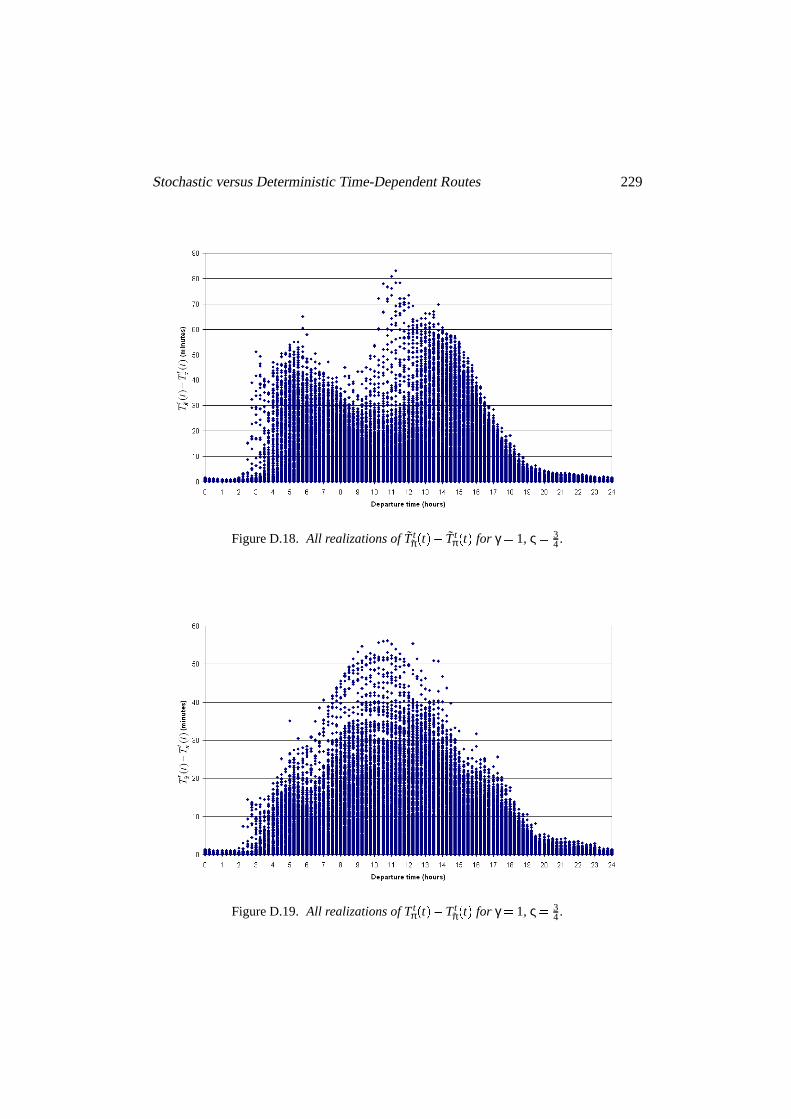
StochasticversusDeterministicTime-DependentRoutes 229
FigureD.18. All realizationsof Ttπ µ t ¶W· Tt
π µ t ¶ for γ ¸ 1, ς ¸ 34.
FigureD.19. All realizationsof Ttπ µ t ¶W· Tt
π µ t ¶ for γ ¸ 1, ς ¸ 34.

230 StochasticversusDeterministicTime-DependentRoutes
FigureD.20. Distributionof Ttπ µ t ¶¤· Tt
π µ t ¶ for γ ¸ 1, ς ¸ 34 at 7:00h,10:30h,16:30h.
FigureD.21. Distributionof Ttπ µ t ¶¤· Tt
π µ t ¶ for γ ¸ 1, ς ¸ 34 at 7:00h,10:30h,16:30h.

StochasticversusDeterministicTime-DependentRoutes 231
FigureD.22. Averageof Ttπ µ t ¶W· Tt
π µ t ¶ andTtπ µ t ¶W· Tt
π µ t ¶ for γ ¸ 1, ς ¸ 3.
FigureD.23. Standard deviationof Ttπ µ t ¶©· Tt
π µ t ¶ andTtπ µ t ¶©· Tt
π µ t ¶ for γ ¸ 1, ς ¸ 3.
FigureD.24. Maximumof Ttπ µ t ¶W· Tt
π µ t ¶ andTtπ µ t ¶W· Tt
π µ t ¶ for γ ¸ 1, ς ¸ 3.

232 StochasticversusDeterministicTime-DependentRoutes
FigureD.25. All realizationsof Ttπ µ t ¶W· Tt
π µ t ¶ for γ ¸ 1, ς ¸ 3.
FigureD.26. All realizationsof Ttπ µ t ¶W· Tt
π µ t ¶ for γ ¸ 1, ς ¸ 3.

StochasticversusDeterministicTime-DependentRoutes 233
FigureD.27. Distributionof Ttπ µ t ¶º· Tt
π µ t ¶ for γ ¸ 1, ς ¸ 3 at 7:00h,10:30h,16:30h.
FigureD.28. Distributionof Ttπ µ t ¶º· Tt
π µ t ¶ for γ ¸ 1, ς ¸ 3 at 7:00h,10:30h,16:30h.

234 StochasticversusDeterministicTime-DependentRoutes

Bibliography
ALBER, JOCHEN, HENNING FERNAU , AND ROLF NIEDERMEIER [2003], Graphseparators:a parameterizedview, Journal of Computerand SystemSci-ences67, 808–832.
ARONSON, JAY E. [1989], A survey of dynamicnetwork flows, Annalsof Opera-tionsResearch 20, 1–66.
AZARON, AMIR, AND FARHAD K IANFAR [2003],Dynamicshortestpathin stochas-tic dynamicnetworks:Shiproutingproblem,EuropeanJournalofOperationalResearch 144, 138–156.
BANOS, R., C. GIL, J. ORTEGA , AND F.G. MONTOYA [2004],A parallelmultilevelmetaheuristicfor graphpartitioning,Journal of Heuristics10, 315–336.
BELLMAN, RICHARD [1957], DynamicProgramming, PrincetonUniversityPress,Princeton,New Jersey, UnitedStates.
BELLMAN, RICHARD [1958], On a routingproblem, Quarterlyof AppliedMathe-matics16, 87–90.
BERRY, JONATHAN W., AND MARK K. GOLDBERG [1999], Pathoptimizationforgraphpartitioningproblems,DiscreteAppliedMathematics90, 27–50.
BERTSEKAS, DIMITRI P. [1998], NetworkOptimization:ContinuousandDiscreteModels, AthenaScientific,Nashua,New Hampshire,UnitedStates.
BOLLOBAS, B., AND A.D. SCOTT [2004], Judiciouspartitionsof bounded-degreegraphs,Journal of GraphTheory46, 131–143.
BRIGHTWELL, GRAHAM , AND DOUGLAS B. WEST [2000], Chapter11: Partiallyorderedsets, in: KennethH. Rosen(ed.),Handbookof DiscreteandCombi-natorial Mathematics, CRCPress,London,UnitedKingdom.
CAR, ADRIJANA , HENNY MEHNER, AND GEORGE TAYLOR [1999], Experi-mentingwith Hierarchical Wayfinding, Technicalreport011999,Universityof Newcastleupon Tyne, Departmentof Geomatics,Newcastleupon Tyne,UnitedKingdom.
CHABINI , I . [2002], Algorithms for k-shortestpathsand other routing problemsin time-dependentnetworks, Acceptedfor publicationin TransportationRe-search Part B: Methodological.
CHABINI , I ., AND SHAN LAN [2002], Adaptationsof the Aw algorithm for thecomputationof fastestpathsin deterministicdiscrete-timedynamicnetworks,IEEETransactionson IntelligentTransportationSystems3, 60–74.
235

236 Bibliography
CHAN, EDWARD P.F., AND NING ZHANG [2001], Finding shortestpathsin largenetwork systems, in: Walid G. Aref (ed.), Proceedingsof the ninth ACMInternational Symposiumon Advancesin Geographic Information Systems,Atlanta,Georgia,UnitedStates,ACM Press,160–166.
CHEN, DANNY Z., OVIDIU DAESCU, X IAOBO (SHARON) HU, AND JINHUI XU
[2003], Finding an optimal pathwithout growing the tree, Journal of Algo-rithms49, 13–41.
CHEN, DANNY Z., AND JINHUI XU [2000], Shortestpathqueriesin planargraphs,Proceedingsof thethirty-secondAnnualACM Symposiumon Theoryof Com-puting, Portland,Oregon,UnitedStates,ACM Press,469–478.
CORDONE, ROBERTO, AND FRANCESCO MAFFIOLI [2004], On thecomplexity ofgraphtreepartitionproblems,DiscreteAppliedMathematics134, 51–65.
CUNHA , CLAUDIO BARBIERI DA , AND JOFFRE SWAIT [2000], New dominancecriteriafor thegeneralizedpermanentlabellingalgorithmfor theshortestpathproblemwith time windows on densegraphs, InternationalTransactionsinOperationalResearch 7, 139–157.
DEAN, BRIAN C. [2004], Algorithms for minimum-costpathsin time-dependentnetworkswith waiting policies,Networks44, 41–46.
DIJKSTRA , E.W. [1959], A noteon two problemsin connexion with graphs, Nu-merischeMathematik1, 269–271.
ERTL, GERHARD [1998], Shortestpath calculationin large road networks, ORSpektrum20, 15–20.
FALKNER, JULIE, FRANZ RENDL, AND HENRY WOLKOWICZ [1994], A computa-tionalstudyof graphpartitioning,MathematicalProgramming66, 211–239.
FERNANDEZ-MADRIGAL, JUAN-ANTONIO, AND JAVIER GONZALEZ [2002],Multihierarchicalgraphsearch, IEEE Transactionson Pattern AnalysisandMachineIntelligence24, 103–113.
FIDUCCIA , C.M., AND R.M. MATTEYSES [1982], A linear-time heuristicfor im-proving network partitions,Proceedingsof thenineteenthDesignAutomationConference, LasVegas,Nevada,UnitedStates,IEEEPress,175–181.
FLINSENBERG, INGRID [2003a], Graphpartitioningfor routeplanningin carnavi-gationsystems,Proceedingsof the11’th IAIN World Congress,SmartNavi-gation- SystemsandServices-, Berlin, Germany.
FLINSENBERG, INGRID [2003b], Using turn restrictionsfor fasterrouteplanningwith partitionedroadnetworks, 10th SaintPetersburg InternationalConfer-enceon IntegratedNavigationSystems, SaintPetersburg, Russia,198–206.
FLINSENBERG, INGRID, MARTIJN VAN DER HORST, JOHAN LUKKIEN, AND
JACQUES VERRIET [2004], Creatinggraphpartitionsfor fastoptimumrouteplanning,WSEASTransactionsonComputers 3, 569–574.
FLOYD, ROBERT W. [1962], Algorithm 97 shortestpath, Communicationsof the
Bibliography 237
ACM 5, 345.FORD JR., L.R., AND D.R. FULKERSON [1962], Flows in Networks, Princeton
UniversityPress,Princeton,New Jersey, UnitedStates.FREDERICKSON, GREG N. [1985],Datastructuresfor on-lineupdatingof minimum
spanningtrees,with applications,SIAMJournalonComputing14, 781–798.FRIGIONI , DANIELE [1998],Semidynamicalgorithmsfor maintainingsingle-source
shortestpathtrees,Algorithmica22, 250–274.FU, L IPING [2001], An adaptive routing algorithm for in-vehicle route guidance
systemswith real-timeinformation,TransportationResearch Part B: Method-ological 35, 749–765.
GAO, SONG [2002], Routingproblemsin stochastictime-dependentnetworkswithapplicationsin dynamic traffic assignment, Master’s thesis,MassachusettsInstituteof Technology, Departmentof Civil andEnvironmentalEngineering,Cambridge,Massachusetts,UnitedStates.
GAO, S., AND I . CHABINI [2002], The bestrouting policy problemin stochastictime-dependentnetworks, TransportationResearch Record 1783, 188–196.
GAREY, M ICHAEL R., AND DAVID S. JOHNSON [1979], Computers and In-tractability: A Guideto the Theoryof NP-Completeness, W.H. Freeman&Co,New York, New York, UnitedStates.
GELPERIN, DAVID [1977], On theoptimalityof A w , Artificial Intelligence8, 69–76.GHIANI , GIANPAOLO, FRANCESCA GUERRIERO, GILBERT LAPORTE, AND
ROBERTO MUSMANNO [2003], Real-timevehiclerouting:Solutionconcepts,algorithmsand parallel computingstrategies, EuropeanJournal of Opera-tional Research 151, 1–11.
GLENN, ANDREW M. [2001], Algorithms for the shortestpathproblemwith timewindows andshortestpathreoptimizationin time-dependentnetworks, Mas-ter’s thesis,MassachusettsInstituteof Technology, Departmentof ElectricalEngineeringandComputerScience,Cambridge,Massachusetts,UnitedStates.
GOLSHANI , FOROUZAN, ENRIQUE CORTES-RELLO, AND THOMAS H. HOWELL
[1996], Dynamic route planningwith uncertaininformation, Knowledge-BasedSystems9, 223–232.
GRANAT, JANUSZ, AND FRANCESCA GUERRIERO [2003], The interactive analy-sis of the multicriteria shortestpathproblemby the referencepoint method,EuropeanJournalof Operational Research 151, 103–118.
HART, PETER E., NILS J. NILSSON, AND BERTRAM RAPHAEL [1968], A formalbasisfor the heuristicdeterminationof minimum costpaths, IEEE Transac-tionsof SystemsScienceandCybernetics4, 100–107.
HE, RACHEL R., HENRY X. L IU, ALAIN L. KORNHAUSER, AND BIN RAN [2002],Temporal andSpatialVariability of TravelTime, TechnicalReportUCI-ITS-WP-02-10,Instituteof TransportationStudies,Universityof California,Irvine,

238 Bibliography
California,UnitedStates.HENZINGER, MONICA R., PHILIP KLEIN, SATISH RAO, AND SAIRAM SUBRA-
MANIAN [1997], Fastershortest-pathalgorithmsfor planargraphs,JournalofComputerandSystemSciences55, 3–23.
HIRAISHI , HIRONORI , HAYATO OHWADA , AND FUMIO M IZOGUCHI [1999], In-tercommunicatingcar navigation systemwith dynamicroute finding, Pro-ceedings1999IEEE/IEEJ/JSAIInternationalConferenceonIntelligentTrans-portationSystems, Tokyo, Japan,IEEE,284–289.
HOFFMANN, ACHIM G. [1994], Thedynamiclocking heuristic- a new graphparti-tioning algorithm, 1994IEEE InternationalSymposiumon CircuitsandSys-tems, London,UnitedKingdom,173–176.
HOLZER, MARTIN [2003], Hierarchicalspeed-uptechniquesfor shortest-pathal-gorithms, Diplomarbeit,Universitat Konstanz,FachbereichInformatik undInformationswissenschaft, Konstanz,Germany.
HOLZER, MARTIN, FRANK SCHULZ, AND THOMAS WILLHALM [2004], Combin-ing speed-uptechniquesfor shortest-pathcomputations,in: CelsoC. RibeiroandSimoneL. Martins (eds.),Experimentaland Efficient Algorithms: ThirdInternationalWorkshop,WEA2004, LectureNotesin ComputerScience3059,AngradosReis,Brazil, Springer, 269–284.
HORN, MARK E. T. [2000], Efficient modelingof travel in networks with time-varyinglink speeds,Networks36, 80–90.
HORST, M.G. VAN DER [2003], Optimalrouteplanningfor carnavigationsystems,Master’s thesis,TechnischeUniversiteitEindhoven,Departmentof Mathemat-icsandComputingScience,Eindhoven,TheNetherlands.
HUANG, YUN-WU, NING JING, AND ELKE A. RUNDENSTEINER [1995], Hierar-chical pathviews: A modelbasedon fragmentationandtransportationroadtypes, Proceedingsof the 3rd ACM InternationalWorkshopon AdvancesinGeographic InformationSystems, Baltimore,Maryland,United States,ACMPress,93–100.
HUANG, YUN-WU, NING JING, AND ELKE A. RUNDENSTEINER [1996], Pathqueriesfor transportationnetworks: dynamicreorderingandsliding windowpagingtechniques,Proceedingsof thefourth ACM Workshopon AdvancesinGeographic InformationSystems, Rockville, Maryland,United States,ACMPress,9–16.
HUANG, YUN-WU, NING JING, AND ELKE A. RUNDENSTEINER [1997], A hier-archicalpathview modelfor pathfinding in intelligenttransportationsystems,GeoInformatica1, 125–159.
HUANG, YUN-WU, NING JING, AND ELKE A. RUNDENSTEINER [2000], Opti-mizing pathqueryperformance:graphclusteringstrategies, TransportationResearch Part C: EmergingTechnologies8, 381–408.

Bibliography 239
JAHN, OLAF, ROLF H. M OHRING, AND ANDREAS S. SCHULZ [2000], Optimalrouting of traffic flows with length restrictionsin networks with congestion,OperationsResearch Proceedings1999, Magdeburg, Germany, Springer.
JING, NING, YUN-WU HUANG, AND ELKE A. RUNDENSTEINER [1996], Hier-archicaloptimizationof optimal pathfinding for transportationapplications,Proceedingsof thefifth InternationalConferenceon InformationandKnowl-edgeManagement, Rockville,Maryland,UnitedStates,ACM Press,261–268.
JING, NING, YUN-WU HUANG, AND ELKE A. RUNDENSTEINER [1998], Hierar-chical encodedpathviews for pathqueryprocessing:An optimal modelandits performanceevaluation,IEEETransactionsonKnowledge andDataEngi-neering10, 409–432.
JOHNSON, ELLIS L. [1972], On shortestpathsandsorting, Proceedingsof the25thACM AnnualConference, Boston,Massachusetts,UnitedStates,510–517.
JUNG, SUNGWON, AND SAKTI PRAMANIK [2002], An efficient pathcomputationmodelfor hierarchicallystructuredtopographicalroadmaps, IEEE Transac-tionson Knowledge andDataEngineering14, 1029–1046.
KAINDL, HERMANN, AND GERHARD KAINZ [1997], Bidirectionalheuristicsearchreconsidered,Journal of Artificial IntelligenceResearch 7, 283–317.
KARGER, DAVID R., AND CLIFFORD STEIN [1996], A new approachto themini-mumcut problem,Journal of theACM 43, 601–640.
KARYPIS, GEORGE, AND V IPIN KUMAR [1998], A fastandhighqualitymultilevelschemefor partitioningirregulargraphs,SIAMJournal on ScientificComput-ing 20, 359–392.
KAUFMAN, DAVID E., AND ROBERT L. SMITH [1993], Fastestpathsin time-dependentnetworksfor intelligentvehicle-highway systemsapplication,IVHSJournal1, 1–11.
KERNIGHAN, B. W., AND S. L IN [1970], An efficientheuristicprocedurefor parti-tioninggraphs,Bell SystemTechnical Journal49, 291–307.
K IM , K IHONG, SEUNGWON YOO, AND SANG K. CHA [1998], A partitioningschemefor hierarchicalpathfindingrobustto link costupdate,Proceedingsofthe5thWorld Congresson ITS, Seoul,Korea.
K IM , YONG-HYUK , AND BYUNG-RO MOON [2004a], Investigationof thefitnesslandscapesin graphbipartitioning: An empirical study, Journal of Heuris-tics 10, 111–133.
K IM , YONG-HYUK , AND BYUNG-RO MOON [2004b], Lock-gainbasedgraphpar-titioning, Journalof Heuristics10, 37–57.
KLEIN, P. N., AND S. SUBRAMANIAN [1998], A fully dynamicapproximationschemefor shortestpathsin planargraphs,Algorithmica22, 235–249.
KRISHNAN, RAJESH, RAM RAMANATHAN, AND MARTHA STEENSTRUP [1999],Optimizationalgorithmsfor large self-structuringnetworks, Proceedingsof

240 Bibliography
the Conferenceon ComputerCommunications(IEEE Infocom), New York,New York, UnitedStates,71–78.
L IPTON, RICHARD J., AND ROBERT ENDRE TARJAN [1979], A separatortheoremfor planargraphs,SIAMJournalon AppliedMathematics36, 177–189.
L IU, HENRY X., WILL RECKER, AND ANTHONY CHEN [2004], Uncovering thecontribution of travel time reliability to dynamicroutechoiceusingreal-timeloopdata,TransportationResearch Part A: Policy andPractice38, 435–453.
MANDOW, L., AND J.L. PEREZ DE LA CRUZ [2003], Multicriteria heuristicsearch,EuropeanJournalof Operational Research 150, 253–280.
MEYER, ULRICH [2001], Single-sourceshortest-pathson arbitrarydirectedgraphsin linear average-casetime, Proceedingsof the twelfth Annual ACM-SIAMSymposiumonDiscreteAlgorithms, Washington,District of Columbia,UnitedStates,Societyfor IndustrialandAppliedMathematics,797–806.
MEYER, ULRICH [2002], Buckets strike back: Improved parallel shortest-paths,Proceedingsof the 16th International Parallel and Distributed ProcessingSymposium, IEEE ComputerSociety, Fort Lauderdale,Florida,UnitedStates.
MEYER, U., AND P. SANDERS [2003], ∆-stepping:a parallelizableshortestpathalgorithm,Journalof Algorithms49, 114–152.
MOHAJER, KEYVAN, ALMIR MUTAPCIC, AND MAJID EMAMI [2004], Estimation-pruning(EP) algorithmfor point-to-pointtravel costminimization in a non-fifo dynamicnetwork, Stanford ElectricalEngineeringandComputerScienceResearch Journal, 4–8, Spring.
MONIEN, BURKHARD, AND RALF DIEKMANN [1997], A local graphpartitioningheuristicmeetingbisectionbounds, Proceedingsof the eighth SIAM Con-ferenceon Parallel Processingfor ScientificComputing, Minneapolis,Min-nesota,UnitedStates,SIAM.
MONIEN, BURKHARD, ROBERT PREIS, AND RALF DIEKMANN [2000], Qualitymatchingand local improvementfor multilevel graph-partitioning, ParallelComputing26, 1609–1634.
MONTEMANNI , R., AND L.M. GAMBARDELLA [2004], An exact algorithm fortherobustshortestpathproblemwith interval data, Computers & OperationsResearch 31, 1667–1680.
MONTEMANNI , R., L.M. GAMBARDELLA , AND A.V. DONATI [2004], A branchandboundalgorithmfor the robust shortestpathproblemwith interval data,OperationsResearch Letters 32, 225–232.
MONTGOMERY, DOUGLAS C., ELIZABETH A. PECK , AND G. GEOFFREY V INING
[2001], Introductionto Linear RegressionAnalysis,3rd Edition, JohnWiley& Sons,New York, New York, UnitedStates.
NARVAEZ, PAOLO, KAI-YEUNG SIU, AND HONG-Y I TZENG [2001], New dy-namicSPTalgorithmbasedon a ball-and-stringmodel, IEEE/ACM Transac-

Bibliography 241
tionson Networking9, 706–718.NGUYEN, SANG, STEFANO PALLOTTINO, AND MARIA GRAZIA SCUTELLA
[2002], A new dual algorithmfor shortestpath reoptimization, in: MichelGendreauandPatriceMarcotte(eds.),TransportationandNetworkAnalysis:Current Trends, Kluwer AcademicPublishers,Dordrecht,The Netherlands,221–235.
ORDA , ARIEL, AND RAPHAEL ROM [1990], Shortest-pathand minimum-delayalgorithms in networks with time-dependentedge-length, Journal of theACM 37, 607–625.
ORDA , ARIEL, AND RAPHAEL ROM [1991], Minimum weight paths in time-dependentnetworks, Networks21, 295–319.
ORDA , ARIEL, AND RAPHAEL ROM [1996], Distributedshortest-pathprotocolsfortime-dependentnetworks, DistributedComputing10, 49–62.
ORLIN, J.B. [1984], Minimum convex costdynamicnetwork flows, MathematicsofOperationsResearch 9, 190–207.
OSOGAMI , TAKAYUKI , AND MOR HARCHOL-BALTER [2003],A closed-formsolu-tion for mappinggeneraldistributionsto minimal PH distributions, ComputerPerformance, LectureNotesin ComputerScience2794,Springer-VerlagHei-delberg, Heidelberg, Germany, 200–217.
PALLOTTINO, STEFANO, AND MARIA GRAZIA SCUTELLA [2003], A new algo-rithm for reoptimizingshortestpathswhenthearc costschange,OperationsResearch Letters 31, 149–160.
PAPE, U. [1974], Implementationandefficiency of Moore-algorithmsfor theshortestrouteproblem,MathematicalProgramming7, 212–222.
PEARL, JUDEA [1984], Heuristics:IntelligentSearch Strategiesfor ComputerProb-lemSolving, Addison-Wesley, Reading,Massachusetts,UnitedStates.
PETTIE, SETH [2002], A fasterall-pairsshortestpathalgorithmfor real-weightedsparsegraphs,Proceedingsof the29thInternationalColloquiumonAutomata,LanguagesandProgramming, LectureNotesin ComputerScience2380,85–97.
POTHEN, ALEX [1997], Graphpartitioningalgorithmswith applicationsto scien-tific computing, in: David E. Keyes,Ahmed Sameh,andV. Venkatakrish-nan(eds.),Parallel NumericalAlgorithms, Kluwer AcademicPublishers,Dor-drecht,Netherlands,323–368.
PREIS, ROBERT [1999], Analytical methodsfor multilevel graph-partitioning, in:Kurt Beiersdorfer, GregorEngels,andWilhelm Schafer(eds.),Informatik’99:InformatikuberwindetGrenzen, Paderborn,Germany, Springer, 223–230.
ROWE, N.C., AND R.S. ALEXANDER [2000], Findingoptimal-pathmapsfor pathplanningacrossweightedregions, TheInternationalJournal of RoboticsRe-search 19, 83–95.

242 Bibliography
SCHLOEGEL, K IRK , GEORGE KARYPIS, AND V IPIN KUMAR [2000], Graphparti-tioning for high performancescientificsimulations,in: J.Dongarra,I. Foster,G. Fox, K. Kennedy, andA. White (eds.),CRPCParallel ComputingHand-book, MorganKaufmann,SanFrancisco,California,UnitedStates.
SCHLOTT, STEFAN [1997], Vehicle navigation: route planning, positioningandrouteguidance, verlagmoderneindustrie,Landsberg/Lech,Germany.
SCHMID, WOLFGANG [2000], BerechnungKurzesterWege in StraßennetzenmitWegeverboten, Dissertation,Universitat Stuttgart,Stuttgart,Germany.
SCHULZ, FRANK , DOROTHEA WAGNER, AND CHRISTOS ZAROLIAGIS [2002],Using multi-level graphsfor timetableinformation in railway systems, Al-gorithmEngineeringandExperiments:4th InternationalWorkshop,ALENEX2002, LectureNotesin ComputerScience2409, SanFrancisco,California,UnitedStates,Springer-Verlag,43–59.
SEONG, MYEONGKI , K ISEOK SUNG, AND SOONDAL PARK [1998], Finding aroutein ahierarchicalurbantransportationnetwork, Proceedingsof 5thWorldCongresson IntelligentTransportSystems, Seoul,Korea.
SHEKHAR, SHASHI , ANDREW FETTERER, AND BRAJESH GOYAL [1997], Mate-rialization trade-offs in hierarchicalshortestpathalgorithms, Proceedingsofthe5th InternationalSymposiumon Large SpatialDatabases, LectureNotesin ComputerScience1262,Berlin, Germany, Springer-Verlag,94–111.
SHEKHAR, SHASHI , AND BABAK HAMIDZADEH [1993], Self-adjustingreal-timesearch:A summaryof results,Proceedingsof theFifth InternationalConfer-enceon Toolswith Artificial Intelligence(ICTAI ’93), Boston,Massachusetts,UnitedStates,IEEE ComputerSociety, 224–231.
SUBRAMANIAN, SHIVARAM [1997], Routing algorithmsfor dynamic,intelligenttransportationnetworks, Master’s thesis,Facultyof theVirginia PolytechnicInstituteandStateUniversity, Blacksburg, Virginia,UnitedStates.
SZEIDER, STEFAN [2003], Finding pathsin graphsavoiding forbiddentransitions,DiscreteAppliedMathematics126, 261–273.
THORUP, M IKKEL [1997], Undirectedsinglesourceshortestpathsin linear time,38thAnnualSymposiumon Foundationsof ComputerScience, Miami Beach,Florida,UnitedStates,IEEE,12–21.
VAN WOENSEL, TOM [2003], Models for uninterruptedtraffic flows: A queue-ing approach, Proefschrift, Universiteit Antwerpen, Faculteit ToegepasteEconomischeWetenschappen,Antwerp,Belgium.
WANG, JINCHANG, AND THOMAS KAEMPKE [2004], Shortestroutecomputationin distributedsystems,Computers & OperationsResearch 31, 1621–1633.
WELLMAN, M ICHAEL, MATTHEW FORD, AND KENNETH LARSON [1995], Pathplanningundertime-dependentuncertainty, Proceedingsof the 11th AnnualConferenceon Uncertaintyin Artificial Intelligence(UAI-95), Montreal,Que-

Bibliography 243
bec,Canada,MorganKaufmannPublishers,532–539.WINTER, STEPHAN [2002], Modeling costsof turnsin routeplanning, GeoInfor-
matica6, 345–361.ZHAO, Y ILIN [1997], VehicleLocationandNavigationSystems, ArtechHouseInc.,
Norwood,Massachusetts,UnitedStates.ZHU, S.Q. [2004], Stochastictime-dependentrouteplanningin carnavigationsys-
tems, Master’s thesis,TechnischeUniversiteit Eindhoven, DepartmentofMathematicsandComputingScience,Eindhoven,TheNetherlands.
ZWILLINGER, DANIEL, AND STEPHEN KOKOSKA (eds.)[1999], CRC StandardProbability andStatisticsTablesandFormulae, CRCPress,London,UnitedKingdom.

244 Bibliography

NotationalIndex
Thenumbersreferto thepagesof thefirst occurrence.
General»6¼0 setof all non-negative realnumbers. . . . . . . . . . . . . . . . . . . . . . . .16
∂ f ½ t ¾∂t first left or right derivative of function f z t | to t . . . . . . . . . . . . .115¿ z S| setof subsetsof setS. . . . . . . . . . . . . . . . . . . . . . . . . . . . . . . . . . . . . 60
ln naturallogarithm. . . . . . . . . . . . . . . . . . . . . . . . . . . . . . . . . . . . . . . 169Pr z A| probabilitythatconditionA holds. . . . . . . . . . . . . . . . . . . . . . . . . 21R2 regressioncoefficient. . . . . . . . . . . . . . . . . . . . . . . . . . . . . . . . . . . . . 97randomz a1 � a2 | a randomrealnumberbetweena1 anda2 . . . . . . . . . . . . . . . . . . . 42
Parametersα averagefractionof evaluatededgesby theAw -algorithm. . . . . .35β thedriver’s aversionagainstuncertaintyin theroutecost. . . . . 22δ detourfactor. . . . . . . . . . . . . . . . . . . . . . . . . . . . . . . . . . . . . . . . . . . . .35ε givenparameterbetween0 and1 . . . . . . . . . . . . . . . . . . . . . . . . . . 21γ thedriver’s desireto arrive no laterthanestimated. . . . . . . . . . .22
ς À_Á eÂv Á eà t  } À_Á eÂv Á eÂς approximatesa travel time’s standarddeviation. . . . 153ζ for estimatingmean/varianceof thetravel time for γ £ 0 . . . . 165
Partition∆ z Ci � Ck1 ��������� CkÀ | changein EE z ϕ � C0 ��������� Ck | by partitioningCi in Ck1 ��������� CkÀ . 63∆ z u � v| Euclideandistancebetweennodeu andv . . . . . . . . . . . . . . . . . . . 42∆1 z Ci � Cj | thechangein EE z G � C1 ��������� Ck | by mergingCi andCj . . . . . . . 50∆3 z Ci � Cj | changein EE z ϕ � C0 ��������� Ck | by mergingCi andCj , i � j � ϕ z 0| 66Φ setof cellscontainingat leastonesubcell. . . . . . . . . . . . . . . . . . .60Φc setof cellsthatdonot containany subcells. . . . . . . . . . . . . . . . . 61ΠM z i � j | priority of merging cellsCi andCj . . . . . . . . . . . . . . . . . . . . . . . . . 48ΠS z u � v| priority of moving nodev to thecell containingnodeu. . . . . . .41δo
1 z e| � δo2 z e| original nodesof edgee � EB in asearchgraphwith Points. . . 81
η all parentcellsthatcontainthestartor destinationnode. . . . . . 99λ thenumberof levelsin amulti-level partition. . . . . . . . . . . . . . . 59
245

246 NotationalIndex
ω z i | cellCω ½ i ¾ containscellCi assubcell. . . . . . . . . . . . . . . . . . . . . . . . 61ϕ z i | setof subcellnumbersof cellCi . . . . . . . . . . . . . . . . . . . . . . . . . . . 60AD averageEuclideandistancefrom startto destinationnode. . . . 35AE z ϕ � C0 ��������� Ck | averagenumberof edgesin amulti-level searchgraph. . . . . . . .62AE z G � C1 ��������� Ck | averagenumberof edgesin asingle-level searchgraph. . . . . . . 34B boundarygraph. . . . . . . . . . . . . . . . . . . . . . . . . . . . . . . . . . . . . . . . . . 28Bi boundarygraphof thepartitionof cellCi . . . . . . . . . . . . . . . . . . . 60bi numberof boundarynodesof cellCi . . . . . . . . . . . . . . . . . . . . . . . 31bi j numberof boundarynodesof thecellCi § Cj . . . . . . . . . . . . . . . 48C z u| cell containingnodeu . . . . . . . . . . . . . . . . . . . . . . . . . . . . . . . . . . . . 32C � Ci acell . . . . . . . . . . . . . . . . . . . . . . . . . . . . . . . . . . . . . . . . . . . . . . . . . . . 28C0 roadgraphbeforecreatingamulti-level partition. . . . . . . . . . . . .60dn z u| correspondingdummynodeof nodeu � NB . . . . . . . . . . . . . . . . .81Ei
B setof boundaryedgesof thepartitionof cellCi . . . . . . . . . . . . . .60E0 edgesof theroadgraphC0 . . . . . . . . . . . . . . . . . . . . . . . . . . . . . . . . .60EB setof boundaryedges. . . . . . . . . . . . . . . . . . . . . . . . . . . . . . . . . . . . 28EB z Ci | boundaryedgesadjacentto anodein cellCi . . . . . . . . . . . . . . . . 43Ei setof edgesof cellCi . . . . . . . . . . . . . . . . . . . . . . . . . . . . . . . . . . . . .28EI z Ci | internaledgesof cellCi . . . . . . . . . . . . . . . . . . . . . . . . . . . . . . . . . . . 30EE z ϕ � C0 ��������� Ck | estimatednumberof evaluationsin amulti-level searchgraph. 62EE z G � C1 ��������� Ck | estimatednumberof evaluationsin asingle-level searchgraph35GS z s� d | � GS searchgraph. . . . . . . . . . . . . . . . . . . . . . . . . . . . . . . . . . . . . . . . . . . . . 32k numberof cells. . . . . . . . . . . . . . . . . . . . . . . . . . . . . . . . . . . . . . . . . . 28Ki Cliquegraphof cellCi . . . . . . . . . . . . . . . . . . . . . . . . . . . . . . . . . . . .76LKn z a1 ��������� an | a loopclique. . . . . . . . . . . . . . . . . . . . . . . . . . . . . . . . . . . . . . . . . . . . . 36MB maximumnumberof boundarynodesof any cell . . . . . . . . . . . . 47mB numberof edgesin theboundarygraph. . . . . . . . . . . . . . . . . . . . .34mB z i � j | numberof boundaryedgesconnectingcellsCi andCj . . . . . . . .48mB z u| numberof boundaryedgesadjacentto nodeu . . . . . . . . . . . . . . . 42MC maximumnumberof neighboringcellsof any cell. . . . . . . . . . .54MD maximumdegreeof anode. . . . . . . . . . . . . . . . . . . . . . . . . . . . . . . 47mi numberof edgesin cellCi . . . . . . . . . . . . . . . . . . . . . . . . . . . . . . . . 34mi z u| numberof internaledgesof cellCi adjacentto nodeu. . . . . . . .42MR maximumnumberof nodeslinkedby positive costrules. . . . . 47Ni
B boundarynodesof thepartitionof cellCi . . . . . . . . . . . . . . . . . . . 60Ni
B z Cj | setof boundarynodesof acellCj , j � ϕ z i | . . . . . . . . . . . . . . . . . 60N0 nodesof theroadgraphC0 . . . . . . . . . . . . . . . . . . . . . . . . . . . . . . . . .60NB setof boundarynodes. . . . . . . . . . . . . . . . . . . . . . . . . . . . . . . . . . . . 28NB z C | setof boundarynodesof cellC . . . . . . . . . . . . . . . . . . . . . . . . . . . . 28Ni setof nodesof cellCi . . . . . . . . . . . . . . . . . . . . . . . . . . . . . . . . . . . . .28

NotationalIndex 247
ni numberof nodesin cellCi . . . . . . . . . . . . . . . . . . . . . . . . . . . . . . . . 34NI z C | internalnodesof cellC . . . . . . . . . . . . . . . . . . . . . . . . . . . . . . . . . . . 30Pi Pointgraphof cellCi . . . . . . . . . . . . . . . . . . . . . . . . . . . . . . . . . . . . . 80Rz u| routegraphof thecell containingnodeu . . . . . . . . . . . . . . . . . . . 32Ri routegraphof cellCi . . . . . . . . . . . . . . . . . . . . . . . . . . . . . . . . . . . . . 31r i numberof routeedgesof cellCi . . . . . . . . . . . . . . . . . . . . . . . . . . . 30rCi usedto denoter i y bi z bi { 1| . . . . . . . . . . . . . . . . . . . . . . . . . . . . . .55
rPi usedto denoter i y 0 . . . . . . . . . . . . . . . . . . . . . . . . . . . . . . . . . . . . . 55
rSi usedto denoter i y min � 2bi � bi z bi { 1|�� . . . . . . . . . . . . . . . . . . . . 55
r i j numberof routeedgesin thecellCi § Cj . . . . . . . . . . . . . . . . . . . .50Si Stargraphof cellCi . . . . . . . . . . . . . . . . . . . . . . . . . . . . . . . . . . . . . . 78SE surfaceof theellipse-shapedsearchareaof theAw -algorithm. 35SM surfaceof themap. . . . . . . . . . . . . . . . . . . . . . . . . . . . . . . . . . . . . . . 35U setof dummynodes. . . . . . . . . . . . . . . . . . . . . . . . . . . . . . . . . . . . . . 88
Planningλ z e| edgeprecedingedgee in theminimum-costroutefrom s to e. 86AE averagenumberof evaluatededges. . . . . . . . . . . . . . . . . . . . . . . . 97CL candidatelist . . . . . . . . . . . . . . . . . . . . . . . . . . . . . . . . . . . . . . . . . . . 189DT detailednetwork . . . . . . . . . . . . . . . . . . . . . . . . . . . . . . . . . . . . . . . . 176H setof unexpandededges. . . . . . . . . . . . . . . . . . . . . . . . . . . . . . . . . . 86h dualfeasibleestimator. . . . . . . . . . . . . . . . . . . . . . . . . . . . . . . . . . . .85hÄ dualfeasibleestimatorfor asearchgraphcontainingPoints. . . 89hw dualfeasibleestimatorfor asearchgraphcontainingStars. . . . 88HLi network consistingof all edgeswith roadclass0 ��������� i . . . . . . 176ST searchtree. . . . . . . . . . . . . . . . . . . . . . . . . . . . . . . . . . . . . . . . . . . . . 189
Profilesz i � bi � fi | costof profile χi . . . . . . . . . . . . . . . . . . . . . . . . . . . . . . . . . . . . . . . . 130Γ setof all profilecosts. . . . . . . . . . . . . . . . . . . . . . . . . . . . . . . . . . . .130χ aprofile. . . . . . . . . . . . . . . . . . . . . . . . . . . . . . . . . . . . . . . . . . . . . . . .129χi the i � 1’th elementin aprofile. . . . . . . . . . . . . . . . . . . . . . . . . . . 129εt maximumerrorin thetravel timeof a time-dependentedge. 136εw maximumerrorin thecostof a time-dependentedge. . . . . . . 137X subsetof profilesapproximatingX . . . . . . . . . . . . . . . . . . . . . . . .132∂t first derivative of t t
e to t . . . . . . . . . . . . . . . . . . . . . . . . . . . . . . . . . . 136∂w first derivative of wt
e to t . . . . . . . . . . . . . . . . . . . . . . . . . . . . . . . . . 137b j minimumcostof profile χ j . . . . . . . . . . . . . . . . . . . . . . . . . . . . . . 129err z χ j � χi � k | therelative errorin theapproximationof χ j
k by χi . . . . . . . . . . 132err z π | maximumerrorin thetravel timeor costof a time-routeπ . . 136

248 NotationalIndex
f z i � j | multiplicationfactorfor χ j if it is approximatedby χi . . . . . . 132f j multiplicationfactorfor profile χi . . . . . . . . . . . . . . . . . . . . . . . . 130n z χ | numberof timeelementsin aprofileminus1 . . . . . . . . . . . . . . 129Ti matchingdeparturetime for elementχi . . . . . . . . . . . . . . . . . . . .131Tχ time interval for whichcosts,speedsor timesarestored. . . . .129Tmax maximumdeparturetime of aprofile. . . . . . . . . . . . . . . . . . . . . .129Tmin minimumdeparturetime of aprofile. . . . . . . . . . . . . . . . . . . . . . 129X setof all profiles. . . . . . . . . . . . . . . . . . . . . . . . . . . . . . . . . . . . . . . . 129
Roadgraphδ1 z e| startnodeof edgee . . . . . . . . . . . . . . . . . . . . . . . . . . . . . . . . . . . . . . 16δ2 z e| endnodeof edgee . . . . . . . . . . . . . . . . . . . . . . . . . . . . . . . . . . . . . . . 16« z e| lengthof edgee. . . . . . . . . . . . . . . . . . . . . . . . . . . . . . . . . . . . . . . . .115d destinationnode. . . . . . . . . . . . . . . . . . . . . . . . . . . . . . . . . . . . . . . . . 16E setof edges. . . . . . . . . . . . . . . . . . . . . . . . . . . . . . . . . . . . . . . . . . . . . .16E z p| � E z G| setof edgesof routep or graphG. . . . . . . . . . . . . . . . . . . . . . . . . .16e� ei edge. . . . . . . . . . . . . . . . . . . . . . . . . . . . . . . . . . . . . . . . . . . . . . . . . . . . 16G a (road)graph. . . . . . . . . . . . . . . . . . . . . . . . . . . . . . . . . . . . . . . . . . . . 16L z p| numberof edgesin routep. . . . . . . . . . . . . . . . . . . . . . . . . . . . . . . .16m numberof edgesin a (road)graph. . . . . . . . . . . . . . . . . . . . . . . . . . 34N setof nodesin a roadgraph. . . . . . . . . . . . . . . . . . . . . . . . . . . . . . . .16n numberof nodesin a roadgraph. . . . . . . . . . . . . . . . . . . . . . . . . . . 16N z p| � N z G| setof nodesof routep or graphG . . . . . . . . . . . . . . . . . . . . . . . . . 16p a route � e1 ��������� e��� . . . . . . . . . . . . . . . . . . . . . . . . . . . . . . . . . . . . . . . .16P z G| setof all routesin G . . . . . . . . . . . . . . . . . . . . . . . . . . . . . . . . . . . . . .16P� z G| setof all routesin G containing« edges. . . . . . . . . . . . . . . . . . . . 16s startnode. . . . . . . . . . . . . . . . . . . . . . . . . . . . . . . . . . . . . . . . . . . . . . . 16u node. . . . . . . . . . . . . . . . . . . . . . . . . . . . . . . . . . . . . . . . . . . . . . . . . . . . 16v node. . . . . . . . . . . . . . . . . . . . . . . . . . . . . . . . . . . . . . . . . . . . . . . . . . . . 16v z e| maximumtravel speededgee . . . . . . . . . . . . . . . . . . . . . . . . . . . . 153we edgecostfunction. . . . . . . . . . . . . . . . . . . . . . . . . . . . . . . . . . . . . . . .16wp routecostfunction. . . . . . . . . . . . . . . . . . . . . . . . . . . . . . . . . . . . . . . 17wwp z G � s� d | costof theoptimumroutefrom nodes to noded in graphG . . 17wr rulecostfunction . . . . . . . . . . . . . . . . . . . . . . . . . . . . . . . . . . . . . . . . 17
StochasticTt
π z t | arrival time of routeπ for departuretime t . . . . . . . . . . . . . . . . . 157Tt
π z t | arrival time of routeπ usingt te z e� t | for departuretime t . . . . . 157
π astochastictime-route. . . . . . . . . . . . . . . . . . . . . . . . . . . . . . . . . . . .21f astochasticfunctionor variable. . . . . . . . . . . . . . . . . . . . . . . . . . . 20

NotationalIndex 249
t te stochastictime-dependentdriving time function. . . . . . . . . . . . .20wt
e stochastictime-dependentedgecostfunction . . . . . . . . . . . . . . . 20µ z x | meanof stochasticvariablex . . . . . . . . . . . . . . . . . . . . . . . . . . . . . . 21µγ meanestimatedtravel time givenparameterγ . . . . . . . . . . . . . . 165Å
preferencerelation. . . . . . . . . . . . . . . . . . . . . . . . . . . . . . . . . . . . . . . 22σ2 z x| varianceof stochasticvariablex . . . . . . . . . . . . . . . . . . . . . . . . . . . 21σγ standarddeviation of theestimatedtravel time for agivenγ . 165c z x | coefficient of variationof stochasticvariablex . . . . . . . . . . . . . . 21Tt
π z t | arrival time of routeπ usingt te z e� t | for departuretime t . . . . . 157
xi realizationi of variablex usedfor explainingavariabley . . . 169yi realizationi of avariabley thatneedsto beexplained. . . . . . .169
Time-dependentπ a time-route. . . . . . . . . . . . . . . . . . . . . . . . . . . . . . . . . . . . . . . . . . . . . 19f t time-dependentfunction f . . . . . . . . . . . . . . . . . . . . . . . . . . . . . . . . 18t time . . . . . . . . . . . . . . . . . . . . . . . . . . . . . . . . . . . . . . . . . . . . . . . . . . . . 18T z e� d � t | minimumtravel time from edgee to noded departingat t . . . 108Tp z t | arrival time of routep for departuretime t . . . . . . . . . . . . . . . . . 121Tt
p z t | arrival time of routep usingv z e� t | for departuretime t . . . . . 121Tπ z t | arrival time of time-routeπ usingv z e| for departuretime t . . 121Tt
π z t | arrival time of time-routeπ for departuretime t . . . . . . . . . . . . 121t te driving time function. . . . . . . . . . . . . . . . . . . . . . . . . . . . . . . . . . . . . 18t tr turningtime function. . . . . . . . . . . . . . . . . . . . . . . . . . . . . . . . . . . . . 18wt
e time-dependentedgecostfunction. . . . . . . . . . . . . . . . . . . . . . . . . 18wt
r time-dependentrulecostfunction. . . . . . . . . . . . . . . . . . . . . . . . . .18

250 NotationalIndex

Author Index
AAlber, J. . . . . . . . . . . . . . . . . . . . . . . . . . 9Alexander, R.S.. . . . . . . . . . . . . . . . . .10Aronson,J.E.. . . . . . . . . . . . . . . . . . 110Azaron,A. . . . . . . . . . . . . . . . . . . . . . . 10
BBanos,R. . . . . . . . . . . . . . . . . . . . . . . . 10Bellman,R.. . . . . . . . .7, 107,141,148Berry, J.W. . . . . . . . . . . . . . . . . . . . . . . . 9Bertsekas,D.P. . . . . . . . . . . . . . . . . . . . 7Bollobas,B. . . . . . . . . . . . . . . . . . . . . .10Brightwell, G. . . . . . . . . . . . . . . . . . . . 22
CCar, A. . . . . . . . . . . . . . . . . . . . . . . . . . . .9Cha,S.K. . . . . . . . . . . . . . . . . . . . . . . . . 9Chabini,I. . . . . . . . . . . . . . . . . . . 10,110Chan,E.P.F. . . . . . . . . . . . . . . . . . . . . . . 9Chen,A. . . . . . . . . . . . . . . . . . . . . . . .162Chen,D.Z. . . . . . . . . . . . . . . . . . . . . .8, 9Cordone,R. . . . . . . . . . . . . . . . . . . . . . 10Cortes-Rello,E. . . . . . . . . . . . . . . . . . 11Cunha,C.B. da. . . . . . . . . . . . . . . . . . 10
DDaescu,O. . . . . . . . . . . . . . . . . . . . . . . . 8Dean,B.C.. . . . . . . . . . . . . . . . . . . . .110Diekmann,R. . . . . . . . . . . . . . . . . 10,59Dijkstra,E.W. .3, 7, 8, 27,75,84,106Donati,A.V.. . . . . . . . . . . . . . . . . . . . .11
EEmami,M. . . . . . . . . . . . . . . . . . . . . .110Ertl, G. . . . . . . . . . . . . . . . . . . . . . . . . . . 9
FFalkner, J.. . . . . . . . . . . . . . . . . 9, 33,40Fernandez-Madrigal,J.-A. . . . . . . . . . 9Fernau,H. . . . . . . . . . . . . . . . . . . . . . . . 9Fetterer, A. . . . . . . . . . . . . . . . . . . . . . . . 9Fiduccia,C.M.. . . . . . . . . . . .10,41,71Flinsenberg, I.C.M. 36,48,55,78,87,
97Floyd, R.W. . . . . . . . . . . . . . . . . . . . . . . 7FordJr., L.R. . . . . . . . . . . . . . . . . . . . . . 7Ford,M. . . . . . . . . . . . . . . . 10,147,152Frederickson,G.N.. . . . . . . . . . . . . . .11Frigioni, D. . . . . . . . . . . . . . . . . . . . . . 11Fu,L. . . . . . . . . . . . . . . . . . . . . . . . . . . 10Fulkerson,D.R.. . . . . . . . . . . . . . . . . . .7
GGambardella,L.M. . . . . . . . . . . . . . . .11Gao,S. . . . . . . . . . . . . . . . . . . . . . . . . . 10Garey, M.R. . . . . . . . . . . . . . . . . . . . . . 36Gelperin,D. . . . . . . . . . . . . . . . . . . 7, 24Ghiani,G. . . . . . . . . . . . . . . . . . . . . . . 11Gil, C.. . . . . . . . . . . . . . . . . . . . . . . . . . 10Glenn,A.M. . . . . . . . . . . . . . . . . . 10,11Goldberg, M.K. . . . . . . . . . . . . . . . . . . .9Golshani,F. . . . . . . . . . . . . . . . . . . . . . 11Gonzalez,J.. . . . . . . . . . . . . . . . . . . . . . 9Goyal, B. . . . . . . . . . . . . . . . . . . . . . . . . 9Granat,J. . . . . . . . . . . . . . . . . . . . . . . . . 8Guerriero,F. . . . . . . . . . . . . . . . . . . 8, 11
HHamidzadeh,B. . . . . . . . . . . . . . . . . . 10Harchol-Balter, M. . . . . . . . . . . . . . .145
251

252 Author Index
Hart,P.E. . . . . . . . . . . . . . . . 7, 8, 24,84He,R.R.. . . . . . . . . . . . . . . . . . . . . . . 144Henzinger, M.R. . . . . . . . . . . . . . . . . . . 9Hiraishi,H. . . . . . . . . . . . . . . . . . . . . . 10Hoffmann,A.G. . . . . . . . . . . . . . . . . . 41Holzer, M. . . . . . . . . . . . . . . . . . . . . . . 61Horn,M.E.T. . . . . . . . . . . . . . . . . . . . . 10Horst,M. vander. .36,48,49,54,68,
98,188Howell, H.H. . . . . . . . . . . . . . . . . . . . . 11Hu, X.S. . . . . . . . . . . . . . . . . . . . . . . . . . 8Huang,Y.-W. . . . . . . . . . . . . . . . . . . 8, 9
JJahn,O.. . . . . . . . . . . . . . . . . . . . . . . . . .7Jing,N. . . . . . . . . . . . . . . . . . . . . . . . . . . 9Johnson,D.S. . . . . . . . . . . . . . . . . . . . 36Johnson,E.L. . . . . . . . . . . . . . . . . . . . 87Jung,N. . . . . . . . . . . . . . . . . . . . . . . . . . 8Jung,S. . . . . . . . . . . . . . . . . . . . . . . 8, 61
KKaempke,T.. . . . . . . . . . . . . . . . . . . . . .8Kaindl, H. . . . . . . . . . . . . . . . . . . . . . 102Kainz,G. . . . . . . . . . . . . . . . . . . . . . . 102Karger, D.R. . . . . . . . . . . . . . . . . . . . . 41Karypis,G.. . . . . . . . . . . . . . . . . . . . . . 10Kaufman,D.E. . . . . . . . . 106,107,147Kernighan,B.W. . . . . . . . . . . . . . 41,71Kianfar, F. . . . . . . . . . . . . . . . . . . . . . . 10Kim, K. . . . . . . . . . . . . . . . . . . . . . . . . . .9Kim, Y.-H. . . . . . . . . . . . . . . . . . . . . . . 10Klein, P.N. . . . . . . . . . . . . . . . . . . . .9, 11Kokoska,S. . . . . . . . . . . . . . . . 151,155Kornhauser, A.L. . . . . . . . . . . . . . . . 144Krishnan,R. . . . . . . . . . . . . . . . . . . . . 10Kumar, V. . . . . . . . . . . . . . . . . . . . . . . .10
LLan,S. . . . . . . . . . . . . . . . . . . . . . . . . 110Laporte,G.. . . . . . . . . . . . . . . . . . . . . .11Larson,K. . . . . . . . . . . . . . 10,147,152
Lin, S. . . . . . . . . . . . . . . . . . . . . . . 41,71Lipton, R.J.. . . . . . . . . . . . . . . . . . . . . . 9Liu, H.X. . . . . . . . . . . . . . . . . . .144,162Lukkien,J. . . . . . . . . . . . . . . . . . . 36,48
MMaffioli, F. . . . . . . . . . . . . . . . . . . . . . . 10Mandow, L. . . . . . . . . . . . . . . . . . . . . . . 8Mattheyses,R.M. . . . . . . . . . 10,41,71Mehner, H. . . . . . . . . . . . . . . . . . . . . . . . 9Meyer, U. . . . . . . . . . . . . . . . . . . . . . . . . 7Mizoguchi,F. . . . . . . . . . . . . . . . . . . . 10Mohajer, K. . . . . . . . . . . . . . . . . . . . . 110Monien,B. . . . . . . . . . . . . . . . . . . 10,59Montemanni,R. . . . . . . . . . . . . . . . . . 11Montgomery, D.C.. . . . . . . . . . . . . .169Montoya,F.G.. . . . . . . . . . . . . . . . . . . 10Moon,B.-R. . . . . . . . . . . . . . . . . . . . . 10Musmanno,R.. . . . . . . . . . . . . . . . . . .11Mutapcic,A. . . . . . . . . . . . . . . . . . . . 110Mohring,R.H.. . . . . . . . . . . . . . . . . . . .7
NNarvaez,P. . . . . . . . . . . . . . . . . . . . . . .11Nguyen,S.. . . . . . . . . . . . . . . . . . . . .193Niedermeier, R.. . . . . . . . . . . . . . . . . . .9Nilsson,N.J. . . . . . . . . . . . . 7, 8, 24,84
OOhwada,H. . . . . . . . . . . . . . . . . . . . . . 10Orda,A. . . . . . . . . . . . . . . . 10,109,110Orlin, J.B. . . . . . . . . . . . . . . . . . . . . . 110Ortega,J. . . . . . . . . . . . . . . . . . . . . . . . 10Osogami,T. . . . . . . . . . . . . . . . . . . . .145
PPerezdela Cruz,J.L.. . . . . . . . . . . . . .8Pallottino,S.. . . . . . . . . . . . . . .191,193Pape,U. . . . . . . . . . . . . . . . . . . . . . . . . . 7Park,S.. . . . . . . . . . . . . . . . . . . . . . . . . . 9Pearl,J. . . . . . . . . . . . . . . . . . . . . . . 7, 85Peck,E.A. . . . . . . . . . . . . . . . . . . . . . 169

Author Index 253
Pettie,S.. . . . . . . . . . . . . . . . . . . . . . . . . 7Pothen,A. . . . . . . . . . . . . . . . . . . . 10,33Pramanik,S.. . . . . . . . . . . . . . . . . . 8, 61Preis,R. . . . . . . . . . . . . . . . . . . . . . . . . 59
RRamanathan,R. . . . . . . . . . . . . . . . . . 10Ran,B. . . . . . . . . . . . . . . . . . . . . . . . . 144Rao,S. . . . . . . . . . . . . . . . . . . . . . . . . . . 9Raphael,B. . . . . . . . . . . . . . 7, 8, 24,84Recker, W. . . . . . . . . . . . . . . . . . . . . . 162Rendl,F. . . . . . . . . . . . . . . . . . . 9, 33,40Rom,R. . . . . . . . . . . . . . . . 10,109,110Rowe,N.C. . . . . . . . . . . . . . . . . . . . . . 10Rundensteiner, E.A.. . . . . . . . . . . . .8, 9
SSanders,P. . . . . . . . . . . . . . . . . . . . . . . . 7Schloegel,K. . . . . . . . . . . . . . . . . . . . .10Schlott,S.. . . . . . . . . . . . . . . . . . . . . . . .3Schmid,W. . . . . . . . . . . . . . . . . . . . 8, 84Schulz,A.S.. . . . . . . . . . . . . . . . . . . . . .7Schulz,F. . . . . . . . . . . . . . . . . . . . . . . . 61Scott,A.D. . . . . . . . . . . . . . . . . . . . . . . 10Scutella,M.G. . . . . . . . . . . . . . 191,193Seong,M. . . . . . . . . . . . . . . . . . . . . . . . .9Shekhar, S. . . . . . . . . . . . . . . . . . . . 9, 10Siu,K.-Y. . . . . . . . . . . . . . . . . . . . . . . . 11Smith,L.R. . . . . . . . . . . . 106,107,147Steenstrup,M. . . . . . . . . . . . . . . . . . . .10Stein,C. . . . . . . . . . . . . . . . . . . . . . . . . 41Subramanian,S.. . . . . . . . . . . . . . .9–11Sung,K. . . . . . . . . . . . . . . . . . . . . . . . . . 9Swait, J. . . . . . . . . . . . . . . . . . . . . . . . . 10Szeider, A. . . . . . . . . . . . . . . . . . . . .8, 84
TTarjan,R.E.. . . . . . . . . . . . . . . . . . . . . . 9Taylor, G. . . . . . . . . . . . . . . . . . . . . . . . . 9Thorup,M. . . . . . . . . . . . . . . . . . . . 7, 24Tzeng,H.-Y. . . . . . . . . . . . . . . . . . . . . 11
VVanWoensel,T. . . 113,116,144,153Verriet,J.. . . . . . . . . . . . . . . . . . . . 36,48Vining, G.G.. . . . . . . . . . . . . . . . . . . 169
WWagner, D. . . . . . . . . . . . . . . . . . . . . . .61Wang,J. . . . . . . . . . . . . . . . . . . . . . . . . . 8Wellman,M.P. . . . . . . . . . 10,147,152West,D.B. . . . . . . . . . . . . . . . . . . . . . . 22Willhalm, T.. . . . . . . . . . . . . . . . . . . . .61Winter, S. . . . . . . . . . . . . . . . . . 8, 33,84Wolkowicz, H. . . . . . . . . . . . . .9, 33,40
XXu, J. . . . . . . . . . . . . . . . . . . . . . . . . . 8, 9
YYoo,S. . . . . . . . . . . . . . . . . . . . . . . . . . . 9
ZZaroliagis,C.. . . . . . . . . . . . . . . . . . . .61Zhang,N. . . . . . . . . . . . . . . . . . . . . . . . . 9Zhao,Y. . . . . . . . . . . . . . . . . . . . . . . . . . 3Zhu,S.Q.. . . . . . . . . . . . . . . . . . . . . . 145Zwillinger, D. . . . . . . . . . . . . . 151,155

254 Author Index

SubjectIndex
Symbols2-partitioning. . . . . . . . . . . . . . . . 41,473-partitioning. . . . . . . . . . . . . . . . . . . 41
AA w -algorithm. . . . . . . . . . . . . . . . 35,84adjacent. . . . . . . . . . . . . . . . . . . . . . . . 16advice. . . . . . . . . . . . . . . . . . . . . . . . . . . 3alternative route. . . . . . . . . . . . . . 4, 194Antwerp. . . . . . . . . . . . . . . . . . . seedataareas. . . . . . . . . . . . . . . . . . . . . . . . . . 176arrival time. . . . . . . . . . . . . . . . . . . . . .19
comparisonaverage. . . . . . . . . . . . . 122,157distribution. . . . . . . . . .124,160maximum. . . . . . . . . . . 122,157standarddeviation . . . 122,157stochastic. . . . . . . . . . . 157–162time-dependent. . . . . . 121–126
pessimistic. . . . . . . . . . . . . . . . .147stochasticroute. . . . . . . . . . . . 157time-dependentroute. . .120,157time-independentroute. . . . . .120
attitudedriver . . . . . . . . . . . . . . . . . . 163approximation. . . . 164,168–172
averagespeed. . . . . . . . . . . . . . . . . . 126Antwerp. . . . . . . . . . . . . . . . . . .114Netherlands. . . . . . . . . . . . . . . .116
Bbonus. . . . . . . . . . . . . . . . . . . . . . . . . 188boundary
edge. . . . . . . . . . . . . . . . . . . . 28,60graph. . . . . . . . . . . . . . . . . . . 28,60
node. . . . . . . . . . . . . . . . . . . . 28,60
CCw -algorithm. . . . . . . . . . . . . . . . .84–87
advantages. . . . . . . . . . . . 182–187complexity . . . . . . . . . . . . . . . . . .87disadvantages. . . . . . . . . 188–189evaluatededges. . . . . . . . . . 90–91
multi-level . . . . . . . . . . . 99–101candidatelist . . . . . . . . . . . . . . . . . . . 189carnavigation. . . . . . . . . . . . . . . . . . . . 2cell . . . . . . . . . . . . . . . . . . . . . . . . . 28,60
ordering. . . . . . . . . . . . . . . . . . . . 60subcell. . . . . . . . . . . . . . . . . . . . . 60time-dependent. . . . . . . . . . . . .127
changecarposition. . . . . . . . . . . . . . . . 193costs. . . . . . . . . . . . . . . . . .190–192destination. . . . . . . . . . . . 193–194location. . . . . . . . . . . . . . . 193–194planningcharacteristic. . . . . . 192progressdriver . . . . . . . . . . . . . 192
city. . . . . . . . . . . . . . . . . . . . . . . . . . . . .28Clique. . . . . . . . . . . . . . . . . . . . . . .74–77
evaluatededges. . . . . . . . . . . . . 96planningwith a. . . . . . . . . . . . . .87time-dependent. . . . . . . . . . . . .128
coefficient of variation. . . . . . . . . . . 21Netherlands. . . . . . . . . . . . . . . .153
complexity . . . . . . . . . . . . . . . . . . 37–40computationtime. . . . . . . . . . . . . . . . 56congestion. . . . . . . . . . . . . . . 6, 10,118consistency . . . . . . . . . . . . . . . .106–110
Antwerp. . . . . . . . . . . . . . . . . . .115
255

256 SubjectIndex
cost . . . . . . . . . . . . . . . . . . 109–110Netherlands. . . . . . . . . . . . . . . .116stochastic. . . . . . . . . . . . . 147–149
Antwerp. . . . . . . . . . . . . . . . .153cost. . . . . . . . . . . . . . . . 148–149Netherlands. . . . . . . . . . . . . .154time. . . . . . . . . . . . . . . . 147–148
time. . . . . . . . . . . . . . . . . . 106–109costfunctions. . . . . . . . . . . . . . . . . . 188cumulative distribution function. .144cyclic route. . . . . . . . . . . . . 75,83,105
Ddata
Antwerp. . . . . . . . . . . . . . 113–115Netherlands. . . . . . . . . . . . . . . .116
motorways. . . . . . . . . . . . . . .117storage. . . . . . . . . . . . . . . . . . . . 188
database. . . . . . . . . . . . . . . . . . . . .5, 178access. . . . . . . . . . . . . . . . . . . . . 187
deadreckoning. . . . . . . . . . . . . . . . . . . 3density. . . . . . . seeprobabilitydensity
functiondeparturetime
maximum. . . . . . . . . . . . . . . . . 129minimum. . . . . . . . . . . . . . . . . . 129
destinationnode. . . . . . . . . . . . . .17,35set. . . . . . . . . . . . . . . . . . . . . . . . . 90
detailednetwork. . . . . . . . . . . . . . . .176detour. . . . . . . . . . . . . . . . . . . . . . . . . . . 4
factor. . . . . . . . . . . . . . . . . . . . . . .35deviation planning. . . . . . . . . . . . . . 193Dijkstra’s algorithm. . . . . . . . . . . 7, 75distribution function. . seecumulative
distribution functiondriver preferences. 5, seealsoattitude
driverdriving time
stochastictime-dependent. . . . 20time-dependent. . . . . . . . . . . . . .18
dualfeasibleestimator. . . . . . . . 85–88
Eedge
cost. . . . . . . . . . . . . . . . . . . . .28,60stochastictime-dependent. . 20time-dependent. . . . . . . . . . . .18time-independent. . . . . . . . . . 16
set. . . . . . . . . . . . . . . . . . . . . . . . . 16ellipse. . . . . . . . . . . . . . . . . . . . . . . . . . 35
surface. . . . . . . . . . . . . . . . . . . . . 35estimatednumberevaluatededges. 36
multi-level . . . . . . . . . . . . . . . . . . 62single-level . . . . . . . . . . . . . . . . . 35
expectation. . . . . . . . . . . . . . . seemeanexpectedtravel time. . . . . . . . .seedata
Ffeasible. . . . . . . . . . . . . .17,20,21,103ferry . . . . . . . . . . . . . . . . . . . . . . . . . . 106first advice. . . . . . . . . . . . . . . . . . . . . . 33
GGPS. . . . . . . . . . . . . . . . . . . . . . . . . . . . . 3graphpartitioning. . . . . . . . . . . . . . . . . 8GSM. . . . . . . . . . . . . . . . . . . . . . . .4, 187guidance. . . . . . . . . . . . . . . . . . . . . . . . . 3gyro. . . . . . . . . . . . . . . . . . . . . . . . . . . . . 3
Hhigh-level network. . . . . . . . . . . . . .176
Iincidentaltraffic jam . . . . . . . 190–191internal
edge. . . . . . . . . . . . . . . . . . . . 28,30memory. . . . . . . . . . . . . . . . . . . . . 5node. . . . . . . . . . . . . . . . . . . . 28,30
Jjam. . . seecongestion,traffic accident
LLevel-Merging. . . . . . . . . . . . . . . 64–68

SubjectIndex 257
numberof levels. . . . . . . . . . . . .66Level-Splitting. . . . . . . . . . . . . . . 63–64
numberof levels. . . . . . . . . . . . .68linear
interpolation. . . . . . . . . . .131,164regression. . . . . . . . . . . . . 169–172
loop. . . . . . . . . . . . . . . . seecyclic routeloopclique. . . . . . . . . . . . . . . . . . . . . . 36
Mmap
matching. . . . . . . . . . . . . . . . . . . . .3supplier. . . . . . . . . . . . . . . . . . . 182surface. . . . . . . . . . . . . . . . . . . . . 35
maps. . . . . . . . . . . . . . . . . . . . . . . . . . . 54maximum
error . . . . . . . . . . . . . . . . . . . . . . 141speed. . . . . . . . . . . . . . . . seespeed
mean. . . . . . . . . . . . . . . . . . . . . . . . . . . 21memory. . . . . . . seedatabase,internal
memorymerging two cells. . . . . . . . . . . . . . . . 49Merging-Algorithm. . . . . . . . . . .48–54
complexity . . . . . . . . . . . . . . . . . .54computationtime. . . . . . . . . . . . 57flexibility . . . . . . . . . . . . . . . . . . . 50numberof cells. . . . . . . . . . . . . .58quality. . . . . . . . . . . . . . . . . . . . . .58
Min-Cut . . . . . . . . . . . . . . . . . . . . . . . . 41minimum-costpathtree. . . . . . . . . . 11minimum-sizesubset. . . . . . . . . . . 132model
stochastictime-dependent. 20–23time-dependent. . . . . . . . . . 18–20time-independent. . . . . . . . .16–18
moving anode. . . . . . . . . . . . . . . . . . .43multi-graph. . . . . . . . . . . . . . . . . . . . . 16multi-level
partition. . . . . . . . . . . . . . . . . . . . 60searchgraph. . . . . . . . . . . . . . . . . 61
averagenumberof edges. . . 62
NNetherlands. . . . . . . . . . . . . . . . seedatanodeset. . . . . . . . . . . . . . . . . . . . . 16,60
Oobjective value. . . . . . . . . . . . . . . . . . 36
verification. . . . . . . . . . . . . . 97–98order
partial. . . . . . . . . . . . . 22,148,152total . . . . . . . . . . . . . . . . . . . 23,151
Pparent. . . . . . . . . . . . . . . . . . . . . . . . . . 61partialorder. . . . . . . . seeorderpartialpartition. . . . . . . . . . . . . . . . . . . . . . . . 28
criteria . . . . . . . . . . . . . . . . . . . . . 33multi-level . . . . . . . . . . . . . . . . . . 60
numberof routecosts. . . . . . 68quality. . . . . . . . . . . . . . . . . . 33,36
penalty. . . . . . . . . . . . . . . . . . . .188,194Point . . . . . . . . . . . . . . . . . . . . 79–82,88
evaluatededges. . . . . . . . . . . . . 91planningwith a . . . . . . . . . . 88–89time-dependent. . . . . . . . . . . . .128turn restrictions. . . . . . . . . . . . . .82
positioning. . . . . . . . . . . . . . . . . . . . . . . 3pre-processing. . . . . . . . . . . . . . . . 6, 27priority function. . . . . . . . . . . . . .42,48probabilitydensityfunction. . . . . .144profile. . . . . . . . . . . . . . . . 129–132,164
cost. . . . . . . . . . . . . . 130–131,164error. . . . . . . . . . . . . . . . . .132,168minimumcost. . . . . . . . . . . . . .130multiplicationfactor. . . .130,134standarddeviation. . . . . . . . . . 164variance. . . . . . . . . . . . . . . . . . . 164
profilesattitudedriver . . . . . . . . . 164,171identical. . . . . . . . . . . . . . . . . . . 129numberof . . . 130,134–136,164,
167–168

258 SubjectIndex
set. . . . . . . . . . . . . . . . . . . . . . . . 129approximation. . . . . . . 132–133
similar . . . . . . . . . . . . . . . . . . . . 131progressdriver . . . . 4, seealsochange
progress
Rrandomization. . . . . . . . . . . . . . . 42,48RDS-TMC . . . . . . . . . . . . . . . . . . 4, 187re-planning. . . . . . . . . . . . . . . . 189–194regressioncoefficient . . . . . . . . . . . 169Ring. . . . . . . . . . . . . . . . . . . . . . . . . . . .82road
class. . . . . . . . . . . . . . . . . .176,182network. . . . . . . . . . . . . . . . . . . . . .5works. . . . . . . . . . . . . . . . . . . . . 190
roadgraphstochastictime-dependent. . . . 21time-dependent. . . . . . . . . . . . . .19time-independent. . . . . . . . . . . . 17
root . . . . . . . . . . . . . . . . . . . . . . . . . . . 193route
batch. . . . . . . . . . . . . . . . . . . . . . . 90edge. . . . . . . . . . . . . . . . .30,76,79
cost. . . . . . . . . . . . . . . 74,78,79error
cost. . . . . . . . . . . . . . . . 137–139numberof edges. . . . . . . . . 140travel time . 136–137,139–140
final. . . . . . . . . . . . . . . . . . . . . . .177graph. . . . . . . . . . . . . . . . . . . 30,73initial . . . . . . . . . . . . . . . . . . . . . 177stochastictime-dependent. . . . 21
cost. . . . . . . . . . . . . . . . . . . . . . 21estimatedcost. . . . . . . . . . . . . 22optimum. . . . . . . . . . . . . . . . . .23
time-dependent. . . . .19,104–105cost. . . . . . . . . . . . . . . . . . . . . . 19
time-independent. . . . . . . . . . . . 16cost. . . . . . . . . . . . . . . . . . . . . . 17
routeplanning. . . . . . . . . . . . . . . . . . . . 3
RP-algorithm. . . . . . . . . . . . . . 175–177comparison
average-case. . . . . . . . 177–179worst-case. . . . . . . . . . 180–182
searchgraph. . . . . . . . . . . . . . . .176rule . . . . . . . . . . . . . . . . . . . . . . . . . . . . 17
cost. . . . . . . . . . . . . . 28,60,76,78time-dependent. . . . . . . . 18,20time-independent. . . . . . . . . . 17
numberof . . . . . . . . . . . . . . 82,188planningwith . . . . . . . . . . . . . . . 83
in apartition. . . . . . . . . . . . . . 74run. . . . . . . . . . . . . . . . . . . . . . . . . .43,48rural. . . . . . . . . . . . . . . . . . . . . . . . . . . .90
SSw -algorithm. . . . . . . . . . . . . . .149–152
complexity . . . . . . . . . . . . . . . . .151search
area. . . . . . . . . . . . . . . . . . . . . . . . 35tree. . . . . . . . . . . . . . . . . . . . . . . 189
searchgraph. . . . . . . . . . . . . . . . . . . . . 32averagenumberof edges.34,202multi-level. . . . . . . . . . . . . . .61,99
averagenumberof edges. . . 62secondarystorage. . . . . . . . . . . . . . . . . 5sensor. . . . . . . . . . . . . . . . . . . . . . . . . . . 3shortestpath. . . . . . . . . . . . . . . . . . . . . .7speed
maximumtime-independent. . . . . . . . .118
Splitting-Algorithm. . . . . . . . . . .41–47complexity . . . . . . . . . . . . . . . . . .47computationtime. . . . . . . . . . . . 57flexibility . . . . . . . . . . . . . . . . . . . 47numberof cells. . . . . . . . . . . . . .58quality. . . . . . . . . . . . . . . . . . . . . .58
standarddeviationcomparison. . . . . . . . . . . . . . . . 157estimation. . . . . . . . . . . . . . . . . 153
Star. . . . . . . . . . . . . . . . . . . . . . . . . 77–79

SubjectIndex 259
evaluatededges. . . . . . . . . . . . . 96planningwith . . . . . . . . . . . . 87–88time-dependent. . . . . . . . . . . . .128
startnode. . . . . . . . . . . . . . . . . . . .17,35set. . . . . . . . . . . . . . . . . . . . . . . . . 90
stochasticconsistency seeconsistencystoppingcriterion. . . . . . . . . . . . . . . . 43subcell. . . . . . . . . . . . . . . . . . . . . seecell
TTw -algorithm. . . . . . . . . . . . . . 110–111tacho. . . . . . . . . . . . . . . . . . . . . . . . . . . . 3time-dependent. . . . . . . . . . . . . . . . . . 10time-expandednetwork . . . . . . . . . 110time-windows. . . . . . . . . 109,110,148total order. . . . . . . . . . . . seeordertotaltrade-off
expectationversusvariation. 156traffic
accident. . . . . . . . . . . . . . . . . . . 190information. . . . . . . . . . . 4, 6, 187rules. . . . . . . . . . . . . . . . . . . . . . . . .8
travel timedistribution. . . . . . . . . . 144tree. . . . . . . . . . . . . . . . . .seesearchtreeturn restriction. . . . . . . . . . . . . . . . . . . .8turningtime . . . . . . . . . . . . . . . . . 18,20
Uuncertainty. . . . . . . . . . . . . . . . . . . 6, 22
progression. . . . . . . . . . . . . . . . 145unconnectedparts. . . . . . . . . . . . . . . .55upperbound. . . . . . . . . . . . . . . . . . . . 192urban. . . . . . . . . . . . . . . . . . . . . . . . . . . 90
Vvariance. . . . . . . . . . . . . . . . . . . . . . . . 21variation. . seecoefficient of variation
Wwaiting. . . . . . . . . . . . . . . 108,109,147

260 SubjectIndex

CurriculumVitae
Ingrid Flinsenberg was born on 21 July 1977 in Helmond. After receiving herdiploma in 1995 from the athenaeumof the MacropediusCollege in Gemert,shestartedto studyeconometricsat Tilburg University. In 2000shegraduatedwith hon-orsin thefield of operationsresearchaftercompletingherMaster’s thesisonthetopicof queuingtheoryat KPN Research.Subsequently, shestartedasa PhD-studentattheEindhovenEmbeddedSystemsInstituteonthetopicof routeplanningalgorithmsfor car navigation. The researchwas carriedout at SiemensVDO Automotive inEindhoven undersupervisionof Prof. dr. Emile Aarts anddr. JacquesVerriet. Itresultedin severalpatentapplications,presentationsandpublicationsat internationalconferencesandthis thesis.
261

262 CurriculumVitae

Samenvatting
Autofabrikantenbieden steedsvaker standaardeen autonavigatiesysteemaan inhun nieuweauto’s. Dezeautonavigatiesystemen geven de bestuurdergesproken envaak ook visueleadviezenhoe zijn bestemmingbijvoorbeeldzo snel mogelijk tebereiken is. Nadatde bestuurderzijn bestemmingheeft ingegeven, en om begelei-dinggevraagdheeft,moetendezeadviezensnelbepaaldwordenomdatdebestuurdermeteenwil vertrekken en niet wil wachtentot het systeemzijn routebepaaldheeft.Bovendienverwachtde bestuurderniet alleensneladviesmaarook de besteroutenaarzijn bestemming.Gezienhet feit dat de kaartendie gebruiktwordenom dezerouteste bepalensteedsgroterworden,hetwegennetwerkvanheelEuropais tegen-woordigbeschikbaarop CD of DVD, is het zeersnelkunnenbepalenvan optimaleroutesop zeergrotewegennetwerkennogsteedseenuitdaging.
Dit proefschriftbeschrijftalgoritmendie gebruiktkunnenwordenom optimaleroutesop zeergrote wegennetwerken snel te kunnenbepalen. Daarbij wordt nietalleenrekeninggehoudenmetdemaximalesnelheid,maarook metdagelijksecon-gestieop snelwegenen eventueleonzekerheidin de reistijdenals gevolg van dezecongestie.Ook wordende resultatenvan de gepresenteerdealgoritmenvergelekenmetdealgoritmendie gebruiktwordenin commerciele autonavigatiesystemen.Weconcluderendat the gepresenteerdeaanpakresulteertin betereroutesdie snellerbepaaldworden dan in het commerciele VDO Dayton autonavigatiesysteemvanSiemensVDO Automotive datter vergelijking gebruiktis.
Dit resultaatis bereikt door allereersthet wegennetwerkzo goedmogelijk opte delenin regio’s, zo genoemdecellen. Om dit zo goedmogelijk te doenis eenpartitioneringscriterium bepaalddat een goedemaat is voor de snelheidvan hetrouteplanningsalgoritmedatmetbehulpvandezepartitioneringdebesteroutemoetbepalen.Om de bestepartitioneringvolgensdit criterium te bepalenzijn tweebe-naderingsalgoritmenontwikkeld, geımplementeerden getestop verschillendeechtewegennetwerken. Ook is dezeaanpaknog uitgebreiddoor ook cellennogmaalsopte delenwaardoorde routeplanningnog verderversneldwordt. Ook hiervoor zijnweertweealgoritmenontwikkeld waarvan de meestbelovendeis geımplementeerden getest.De resultatenlatenziendatmetbehulpvan dezeaanpakoptimaleroutesop zeergrotewegennetwerkensnelbepaaldkunnenworden.
Vervolgensis ereenmodelopgesteldvoordedagelijksecongestieophetwegen-netwerk,en is, metbehulpvandatabetreffendedagelijksecongestieop desnelweg
263

264 Samenvatting
A1/E19nabij Antwerpenin 1995enop debelangrijkstesnelwegenin Nederlandin2002,bepaaldwat het effect is van dezecongestieop de aankomsttijd van de be-stuurderen op de besteroute gegeven dezecongestie. Gebleken is dat vooral indespitsurendoor rekeningte houdenmetdezecongestietijdenshetbepalenvandebesteroute,eenbehoorlijke reductiein deverwachteaankomsttijdtebehalenis. Ver-volgensis eenaanpakvoorgesteldom,ook wanneergebruikwordt gemaaktvaneenpartitie,routestekunnenbepalenvangoedekwaliteit zonderal teveeldatatemoetenopslaan.
Daarnaastis ook het effect van onzekerheidin de reistijdenop de aankomsttijdvan de bestuurderen de besteroutebestudeerd.Hierbij hebbenwe de besteroutezo gedefinieerddat eenbestuurderkan aangeven hoeveel belanghij hechtaanhetnietoverschrijdenvandeverwachteaankomsttijdenaandeonzekerheidin dezeaan-komsttijd. Ook hierbij is gebruikgemaaktvan databetreffendeonzekerheidin dereistijdenopNederlandsesnelwegenin 2002.Uit deresultatenis geblekendatvooralwanneerdebestuurdererg veelwaardehechtaanzekerheidomtrentzijn (laatstmo-gelijke) aankomsttijd,hetmeenemenvaninformatiebetreffendeonzekerheidin reis-tijden zinvol is. Om ook dit te kunnencombinerenmethetgebruikvaneenpartitieis eenaanpakvoorgesteldwaarmeewederomgoedekwaliteit routeskunnenwordenbepaaldzonderdatteveeldatamoetwordenopgeslagenom dit te bereiken.
Tot slot zijn de resultatenvan de voorgesteldealgoritmenvergeleken met dievan algoritmendie gebruikt worden in commerciele autonavigatiesystemen. Hetis gebleken dat de gepresenteerdealgoritmenleiden tot snellererouteplanningenhogerekwaliteit routes.Tevenszijn enigeaanbevelingengedaanoverhoedeoverigefunctionaliteitvanautonavigatiesystemenkanwordengehandhaafdwanneergebruikwordtgemaaktvandevoorgesteldeaanpak.

Titles in the IPA Dissertation Series
J.O. Blanco. TheStateOperator in ProcessAl-gebra. Faculty of MathematicsandComputingScience,TUE. 1996-01
A.M. Geerling. TransformationalDevelopmentof Data-Parallel Algorithms. Faculty of Mathe-maticsandComputerScience,KUN. 1996-02
P.M. Achten. InteractiveFunctionalPrograms:Models,Methods,and Implementation. Facultyof Mathematicsand ComputerScience,KUN.1996-03
M.G.A. Verhoeven. Parallel Local Search. Fac-ulty of Mathematicsand Computing Science,TUE. 1996-04
M.H.G.K. Kesseler. The ImplementationofFunctionalLanguagesonParallel MachineswithDistrib. Memory. Faculty of MathematicsandComputerScience,KUN. 1996-05
D. Alstein. Distributed Algorithms for HardReal-TimeSystems. Facultyof MathematicsandComputingScience,TUE. 1996-06
J.H. Hoepman. Communication,Synchroniza-tion, andFault-Tolerance. Facultyof Mathemat-ics andComputerScience,UvA. 1996-07
H. Doornbos. ReductivityArgumentsand Pro-gramConstruction. Facultyof MathematicsandComputingScience,TUE. 1996-08
D. Turi . Functorial Operational Semanticsandits DenotationalDual. Faculty of MathematicsandComputerScience,VUA. 1996-09
A.M.G. Peeters. Single-RailHandshake Cir-cuits. Faculty of Mathematicsand ComputingScience,TUE. 1996-10
N.W.A. Ar ends. A SystemsEngineeringSpecifi-cation Formalism. Faculty of MechanicalEngi-neering,TUE. 1996-11
P. Severi deSantiago. Normalisationin LambdaCalculusandits Relationto TypeInference. Fac-ulty of Mathematicsand Computing Science,TUE. 1996-12
D.R. Dams. Abstract Interpretation and Par-tition Refinementfor Model Checking. Facultyof Mathematicsand ComputingScience,TUE.1996-13
M.M. Bonsangue. Topological Dualities in Se-mantics. Faculty of MathematicsandComputerScience,VUA. 1996-14
B.L.E. de Fluiter . Algorithms for Graphs ofSmall Treewidth. Faculty of MathematicsandComputerScience,UU. 1997-01
W.T.M. Kars. Process-algebraic Transforma-tions in Context. Faculty of ComputerScience,UT. 1997-02
P.F. Hoogendijk. A Generic Theory of DataTypes. Faculty of MathematicsandComputingScience,TUE. 1997-03
T.D.L. Laan. TheEvolutionof TypeTheoryinLogic andMathematics. Facultyof MathematicsandComputingScience,TUE. 1997-04
C.J. Bloo. Preservationof Terminationfor Ex-plicit Substitution. Faculty of MathematicsandComputingScience,TUE. 1997-05
J.J. Vereijken. Discrete-Time ProcessAlgebra.Facultyof MathematicsandComputingScience,TUE. 1997-06
F.A.M. van den Beuken. A Functional Ap-proach to Syntaxand Typing. Faculty of Math-ematicsandInformatics,KUN. 1997-07
A.W. Heerink. Ins andOutsin RefusalTesting.Facultyof ComputerScience,UT. 1998-01
G. Naumoskiand W. Alberts. A Discrete-EventSimulator for SystemsEngineering. Faculty ofMechanicalEngineering,TUE. 1998-02
J. Verriet . Schedulingwith CommunicationforMultiprocessorComputation. Facultyof Mathe-maticsandComputerScience,UU. 1998-03
J.S.H. van Gageldonk. An AsynchronousLow-Power80C51Microcontroller. Facultyof Math-ematicsandComputingScience,TUE. 1998-04
A.A. Basten. In Termsof Nets: SystemDesignwith Petri Nets and ProcessAlgebra. Facultyof Mathematicsand ComputingScience,TUE.1998-05
E. Voermans. InductiveDatatypeswith Lawsand Subtyping– A Relational Model. Facultyof Mathematicsand ComputingScience,TUE.1999-01

H. ter Doest. TowardsProbabilisticUnification-basedParsing. Faculty of ComputerScience,UT. 1999-02
J.P.L. Segers. Algorithmsfor the SimulationofSurfaceProcesses. Faculty of MathematicsandComputingScience,TUE. 1999-03
C.H.M. van Kemenade. RecombinativeEvolu-tionarySearch. Facultyof MathematicsandNat-ural Sciences,UL. 1999-04
E.I. Barakova. LearningReliability: a StudyonIndecisivenessin SampleSelection. Faculty ofMathematicsandNaturalSciences,RUG. 1999-05
M.P. Bodlaender. Schedulere Optimizationin Real-Time Distributed Databases. Facultyof Mathematicsand ComputingScience,TUE.1999-06
M.A. Reniers. Message SequenceChart: Syn-tax and Semantics. Faculty of MathematicsandComputingScience,TUE. 1999-07
J.P. Warners. Nonlinear approaches to satis-fiability problems. Faculty of MathematicsandComputingScience,TUE. 1999-08
J.M.T. Romijn . AnalysingIndustrial Protocolswith Formal Methods. Facultyof ComputerSci-ence,UT. 1999-09
P.R. D’Ar genio. Algebras and Automata forTimedandStochasticSystems. Facultyof Com-puterScience,UT. 1999-10
G. Fabian. A Language and Simulatorfor Hy-brid Systems. Faculty of MechanicalEngineer-ing, TUE. 1999-11
J. Zwanenburg. Object-OrientedConceptsandProof Rules. Faculty of MathematicsandCom-putingScience,TUE. 1999-12
R.S. Venema. Aspectsof an Integrated NeuralPredictionSystem. Faculty of MathematicsandNaturalSciences,RUG. 1999-13
J. Saraiva. A Purely FunctionalImplementationof AttributeGrammars. Facultyof MathematicsandComputerScience,UU. 1999-14
R. Schiefer. Viper, A VisualisationTool for Par-allel Progam Construction. Faculty of Mathe-maticsandComputingScience,TUE. 1999-15
K.M.M. deLeeuw. CryptologyandStatecraft intheDutch Republic. Facultyof MathematicsandComputerScience,UvA. 2000-01
T.E.J. Vos. UNITY in Diversity. A stratifiedapproach to the verificationof distributedalgo-rithms. Faculty of Mathematicsand ComputerScience,UU. 2000-02
W. Mallon . Theoriesand Tools for the Designof Delay-InsensitiveCommunicatingProcesses.Faculty of Mathematicsand Natural Sciences,RUG. 2000-03
W.O.D. Griffioen . Studiesin ComputerAidedVerification of Protocols. Faculty of Science,KUN. 2000-04
P.H.F.M. Verhoeven. TheDesignof the Math-SpadEditor. Facultyof MathematicsandCom-putingScience,TUE. 2000-05
J. Fey. Design of a Fruit Juice BlendingandPackaging Plant. Faculty of MechanicalEngi-neering,TUE. 2000-06
M. Franssen. Cocktail: A Tool for DerivingCorrect Programs. Faculty of MathematicsandComputingScience,TUE. 2000-07
P.A. Olivier. A Framework for Debugging Het-erogeneousApplications. Faculty of NaturalSciences,Mathematicsand ComputerScience,UvA. 2000-08
E. Saaman. AnotherFormal SpecificationLan-guage. Facultyof MathematicsandNaturalSci-ences,RUG. 2000-10
M. Jelasity. TheShapeof EvolutionarySearchDiscovering and Representing Search SpaceStructure. Faculty of Mathematicsand NaturalSciences,UL. 2001-01
R. Ahn. Agents, Objectsand Eventsa com-putational approach to knowledge, observationandcommunication. Facultyof MathematicsandComputingScience,TU/e. 2001-02
M. Huisman. ReasoningaboutJavaprogramsinhigherorder logic usingPVSandIsabelle. Fac-ulty of Science,KUN. 2001-03
I.M.M.J . Reymen. Improving DesignProcessesthroughStructuredReflection. Facultyof Mathe-maticsandComputingScience,TU/e. 2001-04
S.C.C. Blom. Term Graph Rewriting: syntaxand semantics. Faculty of Sciences,Divisionof Mathematicsand ComputerScience,VUA.2001-05

R. van Lier e. Studiesin Interactive Visualiza-tion. Faculty of NaturalSciences,MathematicsandComputerScience,UvA. 2001-06
A.G. Engels. Languages for Analysisand Test-ing of EventSequences. Facultyof MathematicsandComputingScience,TU/e. 2001-07
J. Hage. Structural Aspects of SwitchingClasses. Faculty of Mathematicsand NaturalSciences,UL. 2001-08
M.H. Lamers. Neural Networksfor AnalysisofData in EnvironmentalEpidemiology: A Case-studyinto AcuteEffectsofAir PollutionEpisodes.Faculty of Mathematicsand Natural Sciences,UL. 2001-09
T.C. Ruys. Towards EffectiveModel Checking.Facultyof ComputerScience,UT. 2001-10
D. Chkliaev. Mechanicalverificationof concur-rency control and recovery protocols. Facultyof Mathematicsand ComputingScience,TU/e.2001-11
M.D. Oostdijk . Generation and presentationof formal mathematicaldocuments. Facultyof Mathematicsand ComputingScience,TU/e.2001-12
A.T. Hofkamp. Reactivemachine control: Asimulation approach using χ. Faculty of Me-chanicalEngineering,TU/e. 2001-13
D. Bosnacki. Enhancingstatespacereductiontechniquesfor modelchecking. Facultyof Math-ematicsandComputingScience,TU/e. 2001-14
M.C. van Wezel. Neural Networksfor Intelli-gent Data Analysis: theoretical and experimen-tal aspects. Facultyof MathematicsandNaturalSciences,UL. 2002-01
V. Bos and J.J.T. Kleijn . Formal Specificationand Analysisof Industrial Systems. Faculty ofMathematicsandComputerScienceandFacultyof MechanicalEngineering,TU/e. 2002-02
T. Kuipers. Techniques for UnderstandingLegacy Software Systems. Faculty of NaturalSciences,Mathematicsand ComputerScience,UvA. 2002-03
S.P. Luttik . ChoiceQuantificationin ProcessAl-gebra. Faculty of NaturalSciences,Mathemat-ics,andComputerScience,UvA. 2002-04
R.J. Willemen. School TimetableConstruction:Algorithmsand Complexity. Faculty of Mathe-maticsandComputerScience,TU/e. 2002-05
M.I.A. Stoelinga. AleaJactaEst: VerificationofProbabilistic,Real-timeandParametricSystems.Faculty of Science,MathematicsandComputerScience,KUN. 2002-06
N. van Vugt. Modelsof Molecular Computing.Faculty of Mathematicsand Natural Sciences,UL. 2002-07
A. Fehnker. Citius, Vilius, Melius: GuidingandCost-Optimalityin ModelCheckingof TimedandHybrid Systems. Facultyof Science,Mathemat-ics andComputerScience,KUN. 2002-08
R. van Stee. On-line Schedulingand Bin Pack-ing. Faculty of Mathematicsand Natural Sci-ences,UL. 2002-09
D. Tauritz . Adaptive Information Filtering:ConceptsandAlgorithms. Facultyof Mathemat-ics andNaturalSciences,UL. 2002-10
M.B. van der Zwaag. Models and Logicsfor ProcessAlgebra. Faculty of Natural Sci-ences, Mathematics, and Computer Science,UvA. 2002-11
J.I. den Hartog. ProbabilisticExtensionsof Se-manticalModels. Faculty of Sciences,Divisionof Mathematicsand ComputerScience,VUA.2002-12
L. Moonen. Exploring Software Systems. Fac-ulty of NaturalSciences,Mathematics,andCom-puterScience,UvA. 2002-13
J.I. van Hemert. ApplyingEvolutionaryCompu-tation to Constraint Satisfactionand Data Min-ing. Faculty of Mathematicsand Natural Sci-ences,UL. 2002-14
S. Andova. ProbabilisticProcessAlgebra. Fac-ulty of Mathematics and Computer Science,TU/e. 2002-15
Y.S. Usenko. Linearization in µCRL. Facultyof Mathematicsand ComputerScience,TU/e.2002-16
J.J.D. Aerts. RandomRedundantStorage forVideo on Demand. Faculty of MathematicsandComputerScience,TU/e. 2003-01
M. de Jonge. To Reuseor To BeReused:Tech-niquesfor componentcompositionandconstruc-tion. Facultyof NaturalSciences,Mathematics,andComputerScience,UvA. 2003-02

J.M.W. Visser. GenericTraversal over TypedSourceCodeRepresentations. Facultyof NaturalSciences,Mathematics,and ComputerScience,UvA. 2003-03
S.M. Bohte. SpikingNeural Networks. Facultyof MathematicsandNaturalSciences,UL. 2003-04
T.A.C. Willemse. SemanticsandVerification inProcessAlgebraswith DataandTiming. Facultyof Mathematicsand ComputerScience,TU/e.2003-05
S.V. Nedea. Analysisand Simulationsof Cat-alytic Reactions. Faculty of MathematicsandComputerScience,TU/e. 2003-06
M.E.M. Lijding . Real-timeSchedulingof Ter-tiary Storage. Facultyof ElectricalEngineering,Mathematics& ComputerScience,UT. 2003-07
H.P. Benz. CasualMultimedia ProcessAnno-tation – CoMPAs. Faculty of Electrical Engi-neering,Mathematics& ComputerScience,UT.2003-08
D. Distefano. On Modelchecking the Dynamicsof Object-basedSoftware: a FoundationalAp-proach. Facultyof ElectricalEngineering,Math-ematics& ComputerScience,UT. 2003-09
M.H. ter Beek. Team Automata– A FormalApproach to the Modelingof Collaboration Be-tweenSystemComponents. Faculty of Mathe-maticsandNaturalSciences,UL. 2003-10
D.J.P. Leijen. The λ Abroad – A FunctionalApproach to Software Components. Faculty ofMathematicsandComputerScience,UU. 2003-11
W.P.A.J. Michiels. PerformanceRatiosfor theDifferencing Method. Faculty of MathematicsandComputerScience,TU/e. 2004-01
G.I. Jojgov. Incomplete Proofs and Termsand Their Use in Interactive Theorem Proving.
Faculty of MathematicsandComputerScience,TU/e. 2004-02
P. Frisco. Theory of Molecular Computing–Splicing and Membrane systems. Faculty ofMathematicsandNaturalSciences,UL. 2004-03
S. Maneth. Modelsof TreeTranslation. Facultyof MathematicsandNaturalSciences,UL. 2004-04
Y. Qian. Data Synchronization and Browsingfor HomeEnvironments. Facultyof MathematicsandComputerScienceandFaculty of IndustrialDesign,TU/e. 2004-05
F. Bartels. On Generalised Coinduction andProbabilistic SpecificationFormats. Faculty ofSciences,Division of Mathematicsand Com-puterScience,VUA. 2004-06
L. Cruz-Filipe . ConstructiveReal Analysis:a Type-Theoretical Formalization and Applica-tions. Facultyof Science,MathematicsandCom-puterScience,KUN. 2004-07
E.H. Gerding. AutonomousAgentsin Bargain-ing Games: An Evolutionary InvestigationofFundamentals,Strategies, and BusinessAppli-cations. Faculty of TechnologyManagement,TU/e. 2004-08
N. Goga. Control and SelectionTechniquesfor the AutomatedTestingof ReactiveSystems.Faculty of MathematicsandComputerScience,TU/e. 2004-09
M. Niqui . FormalisingExactArithmetic: Rep-resentations,Algorithms and Proofs. Facultyof Science,MathematicsandComputerScience,RU. 2004-10
A. Loh. Exploring GenericHaskell. Faculty ofMathematicsandComputerScience,UU. 2004-11
I.C.M. Flinsenberg. RoutePlanningAlgorithmsfor Car Navigation. Facultyof MathematicsandComputerScience,TU/e. 2004-12