NASA-CR-205230

r j r--

Research Institute for Advanced Computer ScienceNASA Ames Research Center

Runge-Kutta Methodsfor Linear Ordinary Differential Equations

David W. Zingg and Todd T. Chisholm

University of Toronto Institute for Aerospace Studies

RIACS Technical Report 97.07

July 1997

https://ntrs.nasa.gov/search.jsp?R=19980228171 2018-05-18T03:43:22+00:00Z

Runge-Kutta Methodsfor Linear Ordinary Differential Equations

David W. Zingg and Todd T. Chisholm

University of Toronto Institute for Aerospace Studies

The Research Institute for Advanced Computer Science is operated by Universities Space Research

Association, The American City Building, Suite 2 ! 2, Columbia, MD 21044, (4 !0)730-2656

Work reported herein was supported by the National Aeronautics and Space Administration under Contract NAS2-13721 to the Universities Space Research Association (USRA).

RUNGE-KUTTA METHODS

FOR LINEAR ORDINARY DIFFERENTIAL EQUATIONS

D.W. ZINGG AND T.T. CHISHOLM

Abstract

Three new Runge-Kutta methods are presented for numerical integration of systems of linear

inhomogeneous ordinary differential equations (ODEs) with constant coefficients. Such ODEs

arise in the numerical solution of the partial differential equations governing linear wave

phenomena. The restriction to linear ODEs with constant coefficients reduces the number of

conditions which the coefficients of the Runge-Kutta method must satisfy. This freedom is used

to develop methods which are more efficient than conventional Runge-Kutta methods. A

fourth-order method is presented which uses only two memory locations per dependent variable,

while the classical fourth-order Runge-Kutta method uses three. This method is an excellent

choice for simulations of linear wave phenomena if memory is a primary concern. In addition,

fifth- and sixth-order methods are presented which require five and six stages, respectively, one

fewer than their conventional counterparts, and are therefore more efficient. These methods are

an excellent option for use with high-order spatial discretizations.

Introduction

We consider the numerical integration of large linear inhomogenous systems of ordinary

differential equations in the form

du= Au - g(t) ( 1)

dt

where A is an M by M matrix whose elements depend on neither u nor t, and u and g(t) are

vectors of length M. Such essentially autonomous systems arise in the numerical solution of

partial differential equations (PDEs) governing linear wave phenomena after application of a

spatial discretization such as a finite-difference, finite-volume, or finite-element method.

Examples of such PDEs are the linearized Euler equations governing acoustic waves and the

Maxwell equations governing electromagnetic waves. The elements of A depend on the PDE

and the spatial discretization. The inhomogeneous term g(t) is associated with either a source

term or the boundary conditions. In the context of wave propagation, the system of ODEs is

oftenmildly stiff with theeigenvaluesof A typically lying nearthe imaginaryaxis.

The systemof ODEs arising from the applicationof a spatial discretizationto a systemof

PDEs can be very large, especially in three-dimensionalsimulations. Consequently, the

constraintson themethodsusedfor integratingthesesystemsaresomewhatdifferent from those

which have driven much of the developmentof numericalmethodsfor initial value problems.

Due to their high accuracyand modestmemory requirements,explicit Runge-Kuttamethods

havebecomepopular for simulationsof wavephenomena[5,6,7,15,17]. Third- andfourth-order

methodsrequiring only two memory locationsper dependentvariable are particularly useful

[3,13,14]. This property is easily achievedby a third-orderRunge-Kuttamethod[14], but an

additional stage is required for a fourth-order method [3]. Since the primary cost of the

integration is in the evaluationof the derivative function, and each stagerequiresa function

evaluation,the additional stagerepresentsa significantincreasein expense.For thesamereason,

error checkingis generallynotperformedwhensolvingvery largesystemsof ODEsarising fromthediscretizationof PDEs.

Therehavebeenseveralattemptsto developefficientmethodsfor integratinglinear systems

of ODEs[4,9,10,11]. Thebasicpremiseof thesemethodsis that themajorcostin evaluatingthe

derivativefunction is in forming thematrix A and the vector g(t). In the application considered

here, the simulation of linear wave phenomena, the matrix A is never explicitly formed or

stored. Hence the methods previously proposed for linear systems are not appropriate for this

application.

It is well known that a Runge-Kutta method with p stages has an order of accuracy not

exceeding p [1,2]. For p_<4, methods of order p can be derived with p stages. However, fifth-

and sixth-order methods require at least six and seven stages, respectively. Nine stages are

required for seventh-order accuracy and eleven for eighth-order accuracy [1]. Since the cost for

our application is roughly proportional to the number of stages, this represents a significant

limitation of higher-order Runge-Kutta methods.

Several authors have considered various approximations to reduce the number of stages and

the storage requirements of high-order Runge-Kutta methods. Shanks [12] was able to develop

schemes with a reduced number of stages by requiring only that the accuracy conditions be

approximately satisfied. Zingg et al. [16,17] propose methods with low storage requirements

which are of high order for linear homogeneous ODEs but second-order otherwise. A similar

idea was proposed previously by Lorenz [8].

2

In this paper, we develop Runge-Kutta methods specifically for linear ODEs with constant

coefficients. By removing the constraints imposed by nonlinearity in the derivative function,

high-order Runge-Kutta methods can be derived which are more efficient in some respect than

the classical methods. In the next section, we present a fourth-order method which requires less

memory than the classical fourth-order Runge-Kutta method. We then present fifth- and sixth-

order methods requiring fewer derivative function evaluations per time step than fifth- and

sixth-order Runge-Kutta methods applicable to nonlinear problems.

General Form of an Explicit Runge-Kutta Method

Without loss of generality, we consider the following scalar ODE:

du- f(t,u)

dt

A general p-stage explicit Runge-Kutta method can be written as

k l = f (tn, un)

i-1

ki = f (tn+cih, un+h _aijkj) i = 2, .." ,pj=l

P

Un+l = Un + h _._bikii=1

where h = At is the time step, tn = nh, and u n is an approximation to u (tn).

(2)

(3)

Low-Storage Fourth-Order Method

We consider first the case p = 4. With the constraints

C 2 = a21

c 3 = a31 +a32 (4)

c4 = a41 + a42 +a43

there remain ten parameters. For fourth-order accuracy, there are eight conditions which must

be satisfied. Four of these arise even for linear homogeneous constant-coefficient ODEs. A

further three conditions must be met if the ODEs are inhomogeneous. The final condition is

associatedwith non-constantcoefficientsor nonlinearity. Therefore,fourth-orderRunge-Kutta

methodsarea two-parameterfamily of whichtheclassicalmethodis aparticularchoice.

If we restrict our attentionto linearconstant-coefficientODEs,the numberof conditionsis

reducedto seven.Theseare

4

_,bi = 1i=1

4

___cib i = 1,/2i=2

c2a32b3 + b4(c2a42 + c3a43 ) = 1/6

c2a32a43b4 = 1/24 (5)

4

_.,bi c2 = 1/'3i=2

_,bi c3 = 1/4i=2

b3c2a32+b4(c2a42+c32a43) = 1/12

The reduction in the number of conditions to be satisfied does not permit us to reduce the

number of stages. However, we can obtain reduced storage requirements.

Following the approach of Wray [14], the requirement that only two memory locations be

used imposes the following three constraints:

b l = a41 = a31 (6)

b 2 = a42

With these constraints, only two memory locations are required for both the dependent variable

and the value of the time derivative. Hence the method requires minimal storage even when

compact or spectral methods are used for the spatial discretization. With the memory locations

denoted A and B, the method proceeds as follows.

1. Initially, u. is stored in A, and B is empty.

2. The term k I -" f(tn, Un) is evaluated and stored in B.

3. Thequantityun + ha 31k l, is calculated and stored in A.

4. The quantity un + ha 21k I is calculated and stored in B.

5. The term k2 = f(tn+c 2h, un+ha 21kl) is evaluated and stored in B.

6. The contents of the two memory locations are linearly combined to form

u n + h (a 3jkl +a 32k 2), which is stored in B.

7. With a41 =a31 , another linear combination gives un +h(a41kl+a42k2), which is stored

inA.

8. The term k3 =f[tn+c3 h, un+h(a31kl+a32k2)] is evaluated and stored in B.

9. The contents of the two memory locations are linearly combined to form

u,_ + h (anl k l+a42k2+a43k3), which is stored in B.

I0. With bl =a41 and b2 =a42, another linear combination gives un +h(blkl+b2k2+b3k3),

which is stored in A.

11. The term k4 =f[tn+c4h, un+h(aalkl+a42k2+a43k3)] is evaluated and stored in B.

12. The contents of the two memory locations are linearly combined to form un +j.

With the additional constraints imposed by the low-storage requirement, we are left with

seven parameters to satisfy the seven conditions given in eq. (5). Although this system may

possess more than one solution, the only solution we have found is

a21 =c2=0.69631521002413, c3=0.29441651741,

c4 =0.82502163765, bl =a41 =a31 =0.07801567728325,

a32 =0.21640084013679, b2 =a42 =0.04708870117112,

a43 =0.69991725920066, b 3 =0.47982272993855,

b 4 = 0.39507289160708

Five.Stage Fifth-Order Method

For the case p=5, we have, in addition to the constraints given in eq. (4), the following

condition:

c5 = a51 +a52 +a53 +a54 (7)

Consequently, adding the fifth stage has produced five additional parameters for a total of fifteen.

The coefficients must satisfy the following eleven conditions in order to produce fifth-order

accuracy for linear constant-coefficient ODEs:

5

_,bi = 1i=1

5

___cibi = 1/'2i=2

c2a32b 3 + b4(c2a42 + c3a43 ) + b5(c2a52 + c3a53 + c4a54) = 1/6

c2a32a43b4 + b5[c2(a42a54 + a32a53 ) + c3a43a54 ] = 1/24

c2a32a43a54b5 = 1/120 (8)

5

_ bic 2 = 1/3i=2

__,bi c3 = 1/4i=2

b3c2a32+b4(c2a42+c2a43)+bs(c2a52+c32a53+c42a54) = 1/12

_,bi c4 = 1/5i=2

(b4a42+b3a32+b5a52)c 3 +(b5a53 +b4a43)c 3 +b5a54 c3 = 1/'20

bs[a54(a42 c2 + a43 c2) + a53a32c22] + b4a43a32 c2 = 1/60

Thus a four-parameter family of solutions is obtained. Several different criteria can be

applied in order to choose a method from this family. The following values have been found by

minimizing the L2 norm of a vector containing the coefficients of the method:

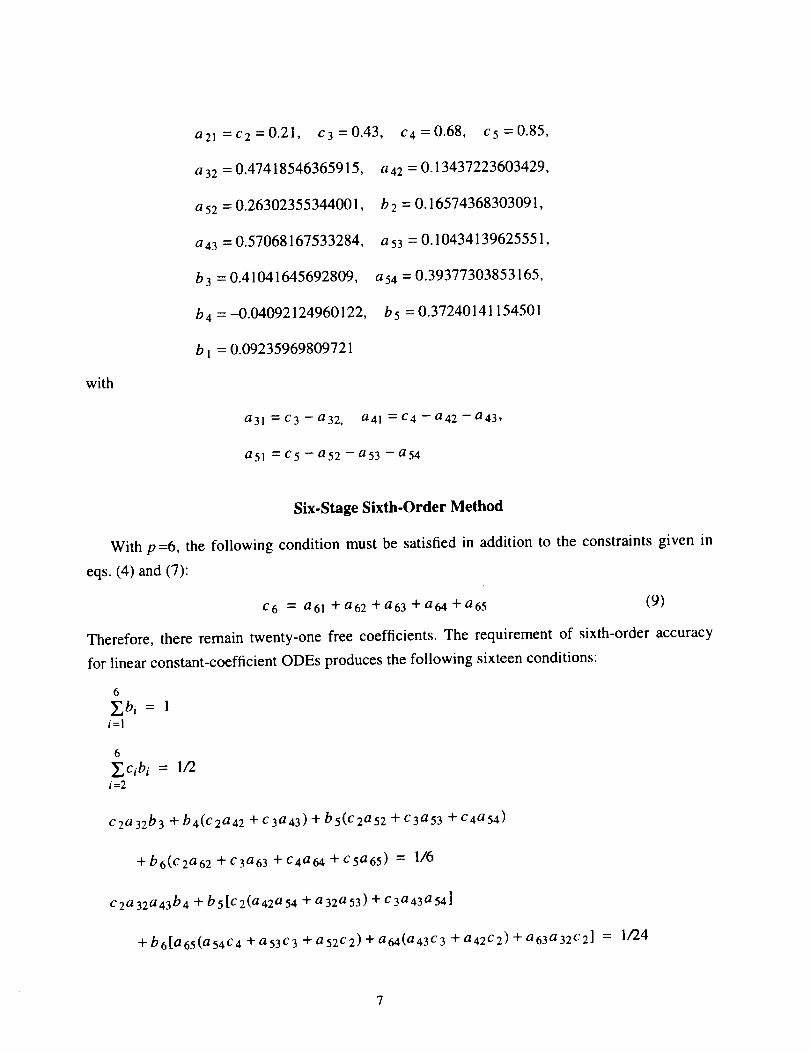
with

a21 - c 2 = 0.21,

a32 = 0.47418546365915,

a 52 = 0.26302355344001,

a 43 = 0.57068167533284,

b 3 = 0.41041645692809,

b 4 ------0.04092124960122,

b I = 0.09235969809721

c3 = 0.43, c 4 = 0.68, c5 = 0.85,

a42 = 0.13437223603429,

b2 = 0.16574368303091,

a53 = 0.10434139625551,

a54 = 0.39377303853165,

b5 = 0.37240141154501

a31 =c 3 -a32 ' a41 =c 4-a42-a43 ,

a51 =c 5-a52-a53-a54

Six-Stage Sixth-Order Method

With p=6, the following condition must be satisfied in addition to the constraints given in

eqs. (4) and (7):

C6 = a61 +a62 +a63 +a64 +a65 (9)

Therefore, there remain twenty-one free coefficients. The requirement of sixth-order accuracy

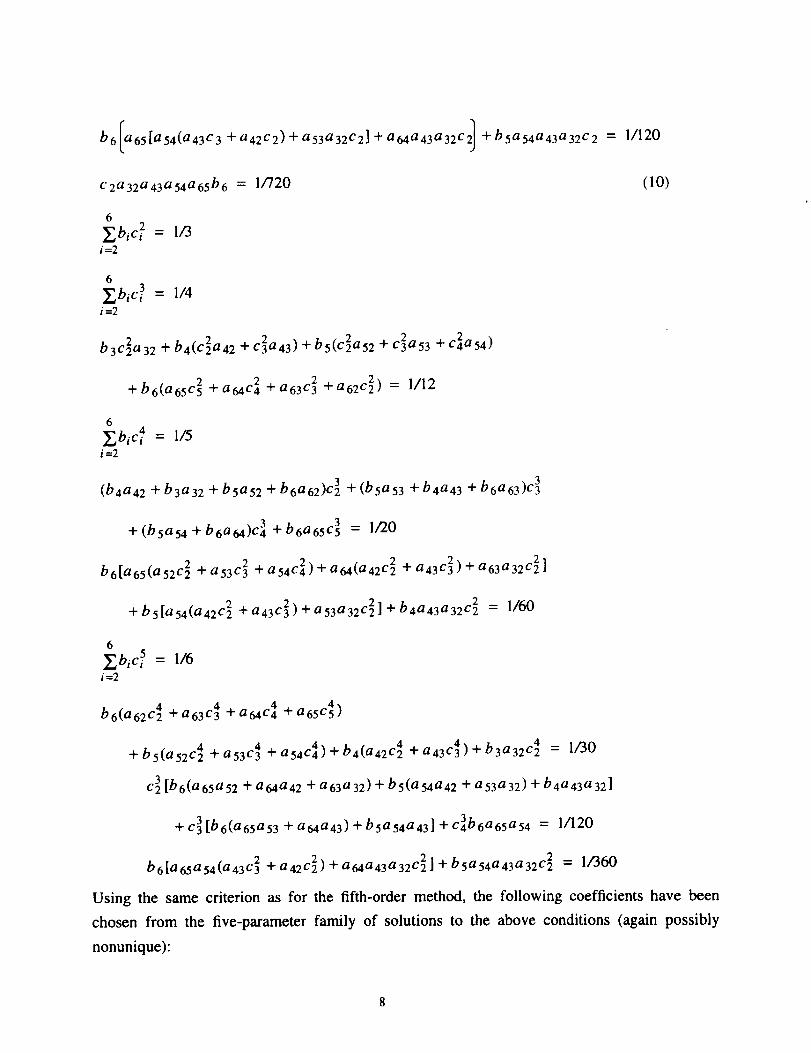
for linear constant-coefficient ODEs produces the following sixteen conditions:

6

_,bi : 1i=1

6

Zcibi-" 1/2i=2

c2a32b 3 + b4(c2a42 + c3a43) + b5(c2a52 + c3a53 + c4a54)

+ b6(c2a62 + c3a63 + c4a64 + c5a65) = 1/6

c 2a 32a43 b4 + b 5 [c 2(a 42 a 54 + a 32a 53 ) + c 3a43 a 54]

+b6[a65(a54c4+a53c 3 +a52c2)+a64(a43c 3 +a42c2)+a63a32c2] = 1/24

b6[a65[a54(a43c3 +a42c2)+a53a32c2]+a64a43a32c21+bsa54a43a32c2

c2a32a43a54a65b6 = 1/720

6

_.,bi c2 = 1/3i=2

6

_._bi c3 = 1/4i=2

b3c2a32 + b4(c2a42 +c2a43)+bs(c2a52 + c2a53 + c2a54)

+b6(a65 c2 +a64 c2 +a63 c2 +a62 c2) = 1/12

6

_,bi c4 = 1/5i =2

(b4a42 + b3a32 + b5a52 + b6a62)c 3 + (b5a53 + b4a43 + b6a63)c 3

+ (b5a54 + b6a64)c34 +b6a65 c3 = 1/20

b 6[a65(a 52c2 + a 53c_ + a s, c 2) + a64(a42 c2 + a43 c2) + a63a 32c2 ]

+ bs[a54(a,2c 2 + a43c 2) + a53a32 c2 ] + b4a43a32 c2 = 1/60

6

_.,bi c5 = 1/6i=2

b6(a62 c4 +a63c_ +a64 c4 +a65 c4)

+bs(a52c4 +a53c4 +a54c4)+b4(a42 c4 +a43c4)+b3a32 c4 = 1/30

c 3 [b6(a65a52 + a64a42 + a63a 32) + b5(a54a42 + a53a32) + b4a43a32]

+ c 3 [b 6(a65a 53 + a64a 43) + b Sa 54a 43] + c3 b 6a65a 54 = 1/120

b6[a65a54(a43 c2 + a42 c2) + a64a43a32 c2 ] + bsa54a43a32 c2 = 1/'360

Using the same criterion as for the fifth-order method, the

chosen from the five-parameter family of solutions to the

nonunique):

= 1/120

(10)

following coefficients have been

above conditions (again possibly

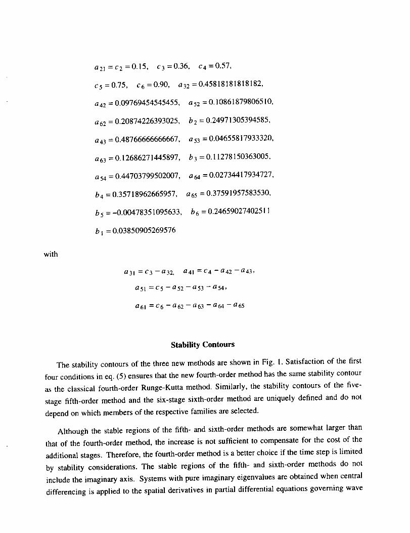
with

a21 =c2=0.15, c3=0.36, c4=0.57,

c5=0.75, c6=0.90, a32=0.45818181818182,

a42 = 0.09769454545455,

a62 = 0.20874226393025,

a43 = 0.48766666666667,

a63 = 0.12686271445897,

a54 = 0.44703799502007,

b 4 = 0.35718962665957,

b5 = -0.00478351095633,

bl = 0.03850905269576

a52 = 0.10861879806510,

b2 = 0.24971305394585,

a53 = 0.04655817933320,

b3 = 0.11278150363005,

am= 0.02734417934727,

a65 = 0.37591957583530,

b6 = 0.24659027402511

a31 =c3-a32, a41 =c4-a42-a43,

a51 =c5-a52-a53-a54,

a61 = c6 - a62 - a63 - a64 - a65

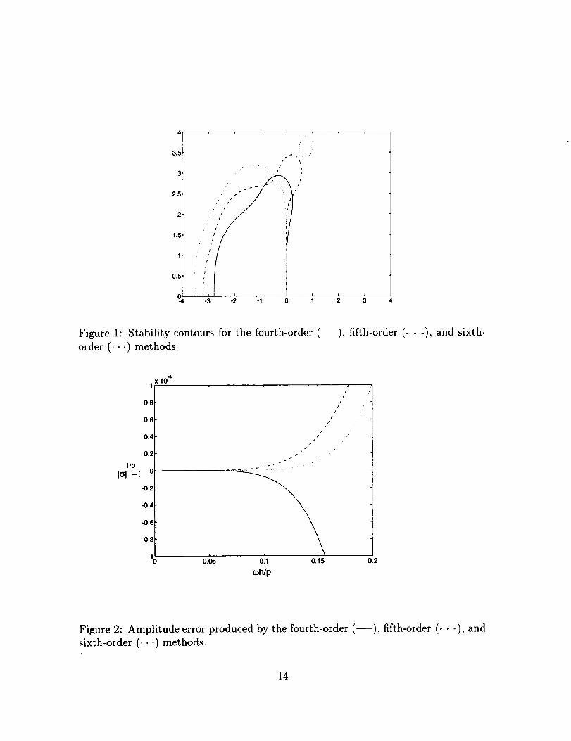
Stability Contours

The stability contours of the three new methods are shown in Fig. 1. Satisfaction of the first

four conditions in eq. (5) ensures that the new fourth-order method has the same stability contour

as the classical fourth-order Runge-Kutta method. Similarly, the stability contours of the five-

stage fifth-order method and the six-stage sixth-order method are uniquely defined and do not

depend on which members of the respective families are selected.

Although the stable regions of the fifth- and sixth-order methods are somewhat larger than

that of the fourth-order method, the increase is not sufficient to compensate for the cost of the

additional stages. Therefore, the fourth-order method is a better choice if the time step is limited

by stability considerations. The stable regions of the fifth- and sixth-order methods do not

include the imaginary axis. Systems with pure imaginary eigenvalues are obtained when central

differencing is applied to the spatial derivatives in partial differential equations governing wave

propagationphenomenawith no physical dissipation,in the absenceof boundaryconditions.

However, Zingg et al. [17] have demonstratedthat by adding a small amountof numerical

dissipationto thespatialdiscretization,stableschemescanbeobtainedusingsuchmethods.The

amountof dissipationrequiredis sufficiently low thatthe overall accuracyof the schemeis not

compromised.The stability contourof themethodsuccessfullyusedin [7] for simulationsof the

propagationandscatteringof electromagneticwavesis identicalto thatof thepresentsixth-ordermethod.

Fourier Error Analysis

Using Fourier analysis we can determine the errors produced by an integration method when

applied to a linear homogeneous ODE. Since our interest is in wave propagation, we consider a

scalar ODE of the form

du-- = it.ou (11)dt

where _ is a real constant. The Runge-Kutta methods developed here produce a solution in the

form

un = OnUo (12)

where

P 1(Y = _ -£-((i0)) k (13)

k--O " "

and p is the number of stages. The local amplitude and phase errors are determined from _ as

follows

era = Iol - 1 (14)

erp=tan -1 (allOt)

coh+ l (15)

where ar and (Yidenote the real and imaginary parts of t_.

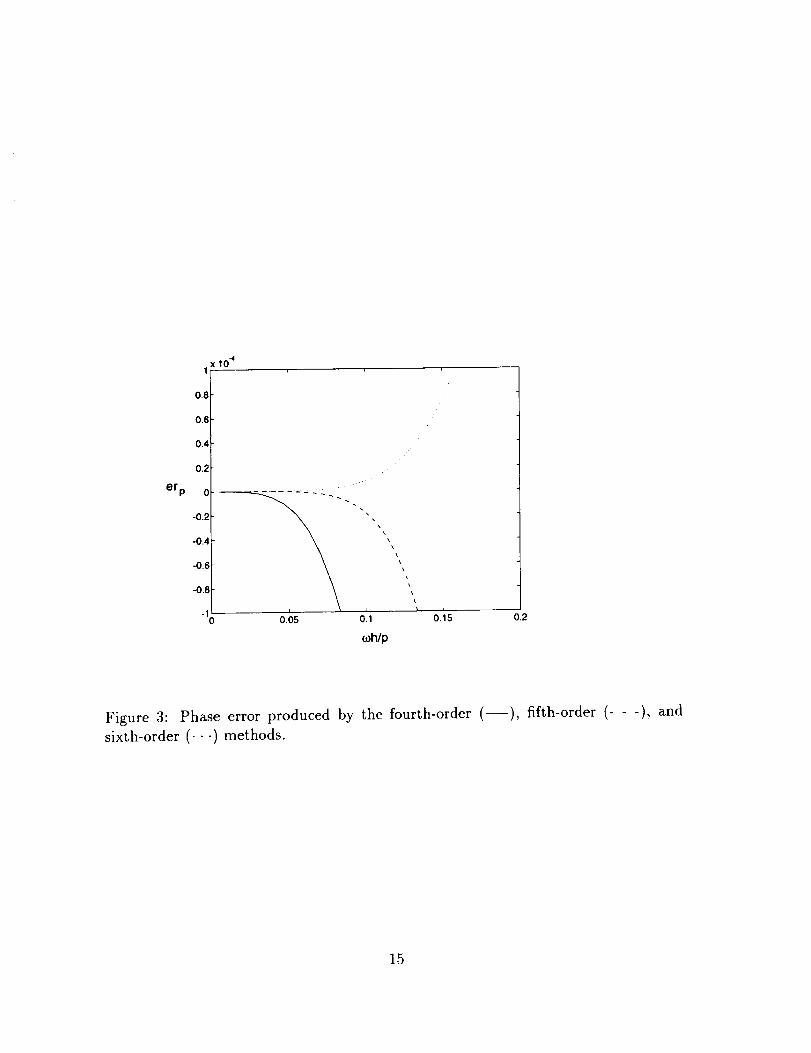
Figs. 2 and 3 show the local amplitude and phase errors produced by the three new methods.

In order to account for the number of stages, the errors are plotted versus toh/p. Hence the errors

shown are for approximately equal computational effort. Since the time step is thus proportional

to p, the amplitude error shown is I_ I l/p_ 1. The figures show that each increase in the order of

the method produces an increase in accuracy even though the extra work has been accounted for.

Hencethefifth- andsixth-ordermethodscanbemoreefficient thanthe fourth-ordermethodif a

sufficiently accuratespatialdiscretizationis used.

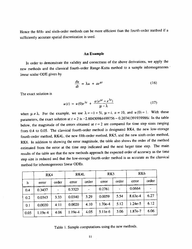
An Example

In order to demonstrate the validity and correctness of the above derivations, we apply the

new methods and the classical fourth-order Runge-Kutta method to a sample inhomogeneous "

linear scalar ODE given by

The exact solution is

du-- = _,u + ae lat (16)dt

u(t) = u(O)e _'t + a(ep't-eXt) (17)IX- _,

when IX_:_,. For the example, we use )_=-I +5i, Ix=i, a = I0, and u(0)= I. With these

parameters, the exact solution at t = 2 is -2.60430984499756- 0.20741391939986i. In the table

below, the magnitude of the errors obtained at t = 2 are compared for time step sizes ranging

from 0.4 to 0.05. The classical fourth-order method is designated RK4, the new low-storage

fourth-order method, RK4L, the new fifth-order method, RK5, and the new sixth-order method,

RK6. In addition to showing the error magnitude, the table also shows the order of the method

estimated from the error at the time step indicated and the next larger time step. The main

results of the table are that the new methods approach the expected order of accuracy as the time

step size is reduced and that the low-storage fourth-order method is as accurate as the classical

method for inhomogeneous linear ODEs.

h

0.4

0.2

0.1

0.05

RK4 RK4L RK5 RK6

error order error order error order error order

0.3437 - 0.3323 - 0.2761 - 0.0664

0.0343 3.33 0.0340 3.29 0.0059 5.54 8.63e-4 6.27

0.0020 4.11 0.0020 4.10 1.70e-4 5.12 1.24e-5 6.12

1.19e-4 4.06 1.19e-4 4.05 5.11 e-6 5.06 1.87e-7 6.06

Table I. Sample computations using the new methods.

II

Conclusions

Three new Runge-Kutta methods have been presented for the integration of linear systems of

ODEs with constant coefficients. If the time step size is limited by stability, then the new

fourth-order method is the most suitable of the new methods. This method requires less memory

than the classical fourth-order Runge-Kutta method and less computational effort than the low-

storage method proposed in [3]. If the time step is limited by accuracy, and memory is a

secondary concern, then the new fifth- and sixth-order methods present an efficient new

alternative. Since the expense of the methods is roughly proportional to the number of stages for

the problems of interest here, the new fifth- and sixth-order methods are significantly more

efficient than their counterparts for nonlinear ODEs. The sixth-order method is a particularly

good choice for use with high-order spatial discretizations.

References

o

,

.

.

.

*

o

J.C. BUTCHER, The Non-Existence of Ten Stage Eighth Order Explicit Runge-Kutta

Methods, BIT 25 (1985), 521-540.

J.C. BUTCHER, The Numerical Analysis of Ordinary Differential Equations, Wiley,

1987.

M.H. CARPENTER AND C.A. KENNEDY, Fourth-Order 2N-Storage Runge-Kutta

Schemes, NASA TM 109112, June 1994.

W.H. ENRIGHT, The Efficient Solution of Linear Constant-Coefficient Systems of

Differential Equations, Simulation, 30 (1978), pp. 129-133.

Z. HARAS AND S. TA'ASAN, Finite-Difference Schemes for Long-Time Integration, J.

Comp. Phys., 114 (1994), pp. 265-279.

F.Q. HU, M.Y. HUSSAINI, AND J.L. MANTHEY, Low-Dissipation and Low-Dispersion

Runge-Kutta Schemes for Computational Acoustics, J. Comp. Phys., 124 (1996), pp. 177-.

191.

H. JURGENS AND D.W. ZINGG, Implementation of a High-Accuracy Finite-Difference

Scheme for Linear Wave Phenomena, Proc. of the International Conf. on Spectral and

High Order Methods, Houston, June 1995, published by the Houston J. of Mathematics,

July 1996.

12

8. E.N. LORENZ, An N-Cycle Time-Differencing Scheme for Stepwise Numerical

Integration, Monthly Weather Rev., 99 (1971), pp. 644-648.

,

12.

13.

14.

15.

16.

17.

L. RANDEZ, Optimizing the Numerical Integration of Initial Value Problems in Shooting

Methods for Linear Boundary Value Problems, SIAM J. Sci. Comput., 14 (1993), pp.

860-871.

L.F. SHAMPINE, Cheaper Integration of Linear Systems, Simulation, 20 (1973), p. 17.

L.F. SHAMPINE, Solution of Structured Non-Stiff ODEs, J. of Computational and

Applied Math., 15 (1986) pp. 293-300.

E.B. SHANKS, Higher-Order Approximations of Runge-Kutta Type, NASA TN D-2920,

Sept. 1965.

J.H. WILLIAMSON, Low-Storage Runge-Kutta Schemes, J. Comp. Phys., 35 (1980), pp.

48-56.

A.A. WRAY, Minimal Storage Time Advancement Schemes for Spectral Methods,

manuscript, NASA Ames Research Center (unpublished).

D.W. ZINGG, A Review of High-Order and Optimized Finite-Difference Methods for

Simulating Linear Wave Phenomena, RIACS TR 96.12, July 1996.

D.W. ZINGG, and H. LOMAX, Some Aspects of High-Order Numerical Solutions of the

Linear Convection Equation with Forced Boundary Conditions, AIAA Paper 93-3381, in

Proceedings of the l lth AIAA Computational Fluid Dynamics Conference, American

Institute for Aeronautics and Astronautics, New York, 1993.

D.W. ZINGG, H. LOMAX, and H.M. JURGENS, High-Accuracy Finite-Difference

Schemes for Linear Wave Propagation, SIAM J. on Scientific Computing, 17 (1996), pp.

328-346.

13

4

3"5t

3

2,5

2

1.5

1

0.5

/

i_ _ ":

.' i/ !1

/ "11// //t_ I

/ /

• II

I

I

: I I I

-3 -2 -1 0 1I i

2 3 4

Figure 1: Stability contours for the fourth-order (--), fifth-order (- - -), and sixth-

order (...) methods.

I/p

lal -I

1

0.8

0.6

0.4

0.2

C

-0.2

-0.4

-O.f

-0.8

-10

10 4

/

./

/

1

I

/

//

/

/

/

/

/

/

0.1 0.15

_Wp

/

I

0.05 0.2

Figure 2: Amplitude error produced by the fourth-order (---), fifth-order (- - -), and

sixth-order (...) methods.

14

erp

x lO 41

0.8

0.6

0.4

0.2

o

-o.2

-o.4

-o.6

-o.8

-1

\x

\

0.05 O. 1

coh/p

/

//

I

0.15 0.2

Figure 3: Phase error produced by the fourth-order (--), fifth-order (- - -), and

sixth-order (...) methods.

15

RIACSMail Stop T041-5

NASA Ames Research Center

Moffett Field, CA 94035