Sage 9.1 Reference Manual: Differential Geometry of Curves ... · Sage 9.1 Reference Manual: Differential Geometry of Curves and Surfaces Release 9.1 The Sage Development Team May

Sage 9.1 Reference Manual: DifferentialGeometry of Curves and Surfaces

Release 9.1

The Sage Development Team

May 21, 2020

CONTENTS

1 Differential Geometry of Parametrized Surfaces 1

2 Common parametrized surfaces in 3D. 21

3 Indices and Tables 27

Python Module Index 29

Index 31

i

ii

CHAPTER

ONE

DIFFERENTIAL GEOMETRY OF PARAMETRIZED SURFACES

AUTHORS:

• Mikhail Malakhaltsev (2010-09-25): initial version

• Joris Vankerschaver (2010-10-25): implementation, doctests

class sage.geometry.riemannian_manifolds.parametrized_surface3d.ParametrizedSurface3D(equation,vari-ables,name=None)

Bases: sage.structure.sage_object.SageObject

Class representing a parametrized two-dimensional surface in Euclidian three-space. Provides methods forcalculating the main geometrical objects related to such a surface, such as the first and the second fundamentalform, the total (Gaussian) and the mean curvature, the geodesic curves, parallel transport, etc.

INPUT:

• surface_equation – a 3-tuple of functions specifying a parametric representation of the surface.

• variables – a 2-tuple of intrinsic coordinates (𝑢, 𝑣) on the surface, with 𝑢 and 𝑣 symbolic variables, ora 2-tuple of triples $(u, u_{min}, u_{max})$, $(v, v_{min}, v_{max})$ when the parameter range for thecoordinates is known.

• name – name of the surface (optional).

Note: Throughout the documentation, we use the Einstein summation convention: whenever an index appearstwice, once as a subscript, and once as a superscript, summation over that index is implied. For instance, 𝑔𝑖𝑗𝑔𝑗𝑘

stands for∑︀

𝑗 𝑔𝑖𝑗𝑔𝑗𝑘.

EXAMPLES:

We give several examples of standard surfaces in differential geometry. First, let’s construct an ellipticparaboloid by explicitly specifying its parametric equation:

sage: u, v = var('u,v', domain='real')sage: eparaboloid = ParametrizedSurface3D((u, v, u^2 + v^2), (u, v),'elliptic→˓paraboloid'); eparaboloidParametrized surface ('elliptic paraboloid') with equation (u, v, u^2 + v^2)

When the ranges for the intrinsic coordinates are known, they can be specified explicitly. This is mainly usefulfor plotting. Here we construct half of an ellipsoid:

1

../../../../../../../html/en/reference/structure/sage/structure/sage_object.html#sage.structure.sage_object.SageObject

Sage 9.1 Reference Manual: Differential Geometry of Curves and Surfaces, Release 9.1

sage: u1, u2 = var ('u1, u2', domain='real')sage: coords = ((u1, -pi/2, pi/2), (u2, 0, pi))sage: ellipsoid_eq = (cos(u1)*cos(u2), 2*sin(u1)*cos(u2), 3*sin(u2))sage: ellipsoid = ParametrizedSurface3D(ellipsoid_eq, coords, 'ellipsoid');→˓ellipsoidParametrized surface ('ellipsoid') with equation (cos(u1)*cos(u2),→˓2*cos(u2)*sin(u1), 3*sin(u2))sage: ellipsoid.plot()Graphics3d Object

Standard surfaces can be constructed using the surfaces generator:

sage: klein = surfaces.Klein(); kleinParametrized surface ('Klein bottle') with equation (-(sin(1/2*u)*sin(2*v) -→˓cos(1/2*u)*sin(v) - 1)*cos(u), -(sin(1/2*u)*sin(2*v) - cos(1/2*u)*sin(v) -→˓1)*sin(u), cos(1/2*u)*sin(2*v) + sin(1/2*u)*sin(v))

Latex representation of the surfaces:

sage: u, v = var('u, v', domain='real')sage: sphere = ParametrizedSurface3D((cos(u)*cos(v), sin(u)*cos(v), sin(v)), (u,→˓v), 'sphere')sage: print(latex(sphere))\left(\cos\left(u\right) \cos\left(v\right), \cos\left(v\right)→˓\sin\left(u\right), \sin\left(v\right)\right)sage: print(sphere._latex_())\left(\cos\left(u\right) \cos\left(v\right), \cos\left(v\right)→˓\sin\left(u\right), \sin\left(v\right)\right)sage: print(sphere)Parametrized surface ('sphere') with equation (cos(u)*cos(v), cos(v)*sin(u),→˓sin(v))

To plot a parametric surface, use the plot() member function:

sage: enneper = surfaces.Enneper(); enneperParametrized surface ('Enneper's surface') with equation (-1/9*(u^2 - 3*v^2 -→˓3)*u, -1/9*(3*u^2 - v^2 + 3)*v, 1/3*u^2 - 1/3*v^2)sage: enneper.plot(aspect_ratio='automatic')Graphics3d Object

We construct an ellipsoid whose axes are given by symbolic variables 𝑎, 𝑏 and 𝑐, and find the natural frame oftangent vectors, expressed in intrinsic coordinates. Note that the result is a dictionary of vector fields:

sage: a, b, c = var('a, b, c', domain='real')sage: u1, u2 = var('u1, u2', domain='real')sage: ellipsoid_eq = (a*cos(u1)*cos(u2), b*sin(u1)*cos(u2), c*sin(u2))sage: ellipsoid = ParametrizedSurface3D(ellipsoid_eq, (u1, u2), 'Symbolic→˓ellipsoid'); ellipsoidParametrized surface ('Symbolic ellipsoid') with equation (a*cos(u1)*cos(u2),→˓b*cos(u2)*sin(u1), c*sin(u2))

sage: ellipsoid.natural_frame(){1: (-a*cos(u2)*sin(u1), b*cos(u1)*cos(u2), 0), 2: (-a*cos(u1)*sin(u2), -→˓b*sin(u1)*sin(u2), c*cos(u2))}

We find the normal vector field to the surface. The normal vector field is the vector product of the vectors of thenatural frame, and is given by:

2 Chapter 1. Differential Geometry of Parametrized Surfaces


sage: ellipsoid.normal_vector()(b*c*cos(u1)*cos(u2)^2, a*c*cos(u2)^2*sin(u1), a*b*cos(u2)*sin(u2))

By default, the normal vector field is not normalized. To obtain the unit normal vector field of the ellipticparaboloid, we put:

sage: u, v = var('u,v', domain='real')sage: eparaboloid = ParametrizedSurface3D([u,v,u^2+v^2],[u,v],'elliptic paraboloid→˓')sage: eparaboloid.normal_vector(normalized=True)(-2*u/sqrt(4*u^2 + 4*v^2 + 1), -2*v/sqrt(4*u^2 + 4*v^2 + 1), 1/sqrt(4*u^2 + 4*v^2→˓+ 1))

Now let us compute the coefficients of the first fundamental form of the torus:

sage: u, v = var('u, v', domain='real')sage: a, b = var('a, b', domain='real')sage: torus = ParametrizedSurface3D(((a + b*cos(u))*cos(v),(a + b*cos(u))*sin(v),→˓b*sin(u)),[u,v],'torus')sage: torus.first_fundamental_form_coefficients(){(1, 1): b^2, (1, 2): 0, (2, 1): 0, (2, 2): b^2*cos(u)^2 + 2*a*b*cos(u) + a^2}

The first fundamental form can be used to compute the length of a curve on the surface. For example, let us findthe length of the curve 𝑢1 = 𝑡, 𝑢2 = 𝑡, 𝑡 ∈ [0, 2𝜋], on the ellipsoid with axes 𝑎 = 1, 𝑏 = 1.5 and 𝑐 = 1. So wetake the curve:

sage: t = var('t', domain='real')sage: u1 = tsage: u2 = t

Then find the tangent vector:

sage: du1 = diff(u1,t)sage: du2 = diff(u2,t)sage: du = vector([du1, du2]); du(1, 1)

Once we specify numerical values for the axes of the ellipsoid, we can determine the numerical value of thelength integral:

sage: L = sqrt(ellipsoid.first_fundamental_form(du, du).substitute(u1=u1,u2=u2))sage: numerical_integral(L.substitute(a=2, b=1.5, c=1),0,1)[0] # rel tol 1e-112.00127905972

We find the area of the sphere of radius 𝑅:

sage: R = var('R', domain='real')sage: u, v = var('u,v', domain='real')sage: assume(R>0)sage: assume(cos(v)>0)sage: sphere = ParametrizedSurface3D([R*cos(u)*cos(v),R*sin(u)*cos(v),R*sin(v)],→˓[u,v],'sphere')sage: integral(integral(sphere.area_form(),u,0,2*pi),v,-pi/2,pi/2)4*pi*R^2

We can find an orthonormal frame field {𝑒1, 𝑒2} of a surface and calculate its structure functions. Let us firstdetermine the orthonormal frame field for the elliptic paraboloid:

3


sage: u, v = var('u,v', domain='real')sage: eparaboloid = ParametrizedSurface3D([u,v,u^2+v^2],[u,v],'elliptic paraboloid→˓')sage: eparaboloid.orthonormal_frame(){1: (1/sqrt(4*u^2 + 1), 0, 2*u/sqrt(4*u^2 + 1)), 2: (-4*u*v/(sqrt(4*u^2 + 4*v^2 +→˓1)*sqrt(4*u^2 + 1)), sqrt(4*u^2 + 1)/sqrt(4*u^2 + 4*v^2 + 1), 2*v/(sqrt(4*u^2 +→˓4*v^2 + 1)*sqrt(4*u^2 + 1)))}

We can express the orthogonal frame field both in exterior coordinates (i.e. expressed as vector field fields inthe ambient space R3, the default) or in intrinsic coordinates (with respect to the natural frame). Here we useintrinsic coordinates:

sage: eparaboloid.orthonormal_frame(coordinates='int'){1: (1/sqrt(4*u^2 + 1), 0), 2: (-4*u*v/(sqrt(4*u^2 + 4*v^2 + 1)*sqrt(4*u^2 + 1)),→˓sqrt(4*u^2 + 1)/sqrt(4*u^2 + 4*v^2 + 1))}

Using the orthonormal frame in interior coordinates, we can calculate the structure functions 𝑐𝑘𝑖𝑗 of the surface,defined by [𝑒𝑖, 𝑒𝑗 ] = 𝑐𝑘𝑖𝑗𝑒𝑘, where [𝑒𝑖, 𝑒𝑗 ] represents the Lie bracket of two frame vector fields 𝑒𝑖, 𝑒𝑗 . For theelliptic paraboloid, we get:

sage: EE = eparaboloid.orthonormal_frame(coordinates='int')sage: E1 = EE[1]; E2 = EE[2]sage: CC = eparaboloid.frame_structure_functions(E1,E2)sage: CC[1,2,1].simplify_full()4*sqrt(4*u^2 + 4*v^2 + 1)*v/((16*u^4 + 4*(4*u^2 + 1)*v^2 + 8*u^2 + 1)*sqrt(4*u^2→˓+ 1))

We compute the Gaussian and mean curvatures of the sphere:

sage: sphere = surfaces.Sphere(); sphereParametrized surface ('Sphere') with equation (cos(u)*cos(v), cos(v)*sin(u),→˓sin(v))sage: K = sphere.gauss_curvature(); K # Not tested -- see trac 127371sage: H = sphere.mean_curvature(); H # Not tested -- see trac 12737-1

We can easily generate a color plot of the Gaussian curvature of a surface. Here we deal with the ellipsoid:

sage: u1, u2 = var('u1,u2', domain='real')sage: u = [u1,u2]sage: ellipsoid_equation(u1,u2) = [2*cos(u1)*cos(u2),1.5*cos(u1)*sin(u2),sin(u1)]sage: ellipsoid = ParametrizedSurface3D(ellipsoid_equation(u1,u2), [u1, u2],→˓'ellipsoid')sage: # set intervals for variables and the number of division pointssage: u1min, u1max = -1.5, 1.5sage: u2min, u2max = 0, 6.28sage: u1num, u2num = 10, 20sage: # make the arguments arraysage: from numpy import linspacesage: u1_array = linspace(u1min, u1max, u1num)sage: u2_array = linspace(u2min, u2max, u2num)sage: u_array = [ (uu1,uu2) for uu1 in u1_array for uu2 in u2_array]sage: # Find the gaussian curvaturesage: K(u1,u2) = ellipsoid.gauss_curvature()sage: # Make array of K valuessage: K_array = [K(uu[0],uu[1]) for uu in u_array]

(continues on next page)



(continued from previous page)

sage: # Find minimum and max of the gauss curvaturesage: K_max = max(K_array)sage: K_min = min(K_array)sage: # Make the array of color coefficientssage: cc_array = [ (ccc - K_min)/(K_max - K_min) for ccc in K_array ]sage: points_array = [ellipsoid_equation(u_array[counter][0],u_array[counter][1])→˓for counter in range(0,len(u_array)) ]sage: curvature_ellipsoid_plot = sum( point([xx for xx in points_array[counter]],→˓color=hue(cc_array[counter]/2)) for counter in range(0,len(u_array)) )sage: curvature_ellipsoid_plot.show(aspect_ratio=1)

We can find the principal curvatures and principal directions of the elliptic paraboloid:

sage: u, v = var('u, v', domain='real')sage: eparaboloid = ParametrizedSurface3D([u, v, u^2+v^2], [u, v], 'elliptic→˓paraboloid')sage: pd = eparaboloid.principal_directions(); pd[(2*sqrt(4*u^2 + 4*v^2 + 1)/(16*u^4 + 16*v^4 + 8*(4*u^2 + 1)*v^2 + 8*u^2 + 1),→˓[(1, v/u)], 1), (2/sqrt(4*u^2 + 4*v^2 + 1), [(1, -u/v)], 1)]

We extract the principal curvatures:

sage: k1 = pd[0][0].simplify_full()sage: k12*sqrt(4*u^2 + 4*v^2 + 1)/(16*u^4 + 16*v^4 + 8*(4*u^2 + 1)*v^2 + 8*u^2 + 1)sage: k2 = pd[1][0].simplify_full()sage: k22/sqrt(4*u^2 + 4*v^2 + 1)

and check them by comparison with the Gaussian and mean curvature expressed in terms of the principal cur-vatures:

sage: K = eparaboloid.gauss_curvature().simplify_full()sage: K4/(16*u^4 + 16*v^4 + 8*(4*u^2 + 1)*v^2 + 8*u^2 + 1)sage: H = eparaboloid.mean_curvature().simplify_full()sage: H2*(2*u^2 + 2*v^2 + 1)/(4*u^2 + 4*v^2 + 1)^(3/2)sage: (K - k1*k2).simplify_full()0sage: (2*H - k1 - k2).simplify_full()0

We can find the intrinsic (local coordinates) of the principal directions:

sage: pd[0][1][(1, v/u)]sage: pd[1][1][(1, -u/v)]

The ParametrizedSurface3D class also contains functionality to compute the coefficients of the second funda-mental form, the shape operator, the rotation on the surface at a given angle, the connection coefficients. Onecan also calculate numerically the geodesics and the parallel translation along a curve.

Here we compute a number of geodesics on the sphere emanating from the point (1, 0, 0), in variousdirections. The geodesics intersect again in the antipodal point (-1, 0, 0), indicating that these points areconjugate:

5


sage: S = surfaces.Sphere()sage: g1 = [c[-1] for c in S.geodesics_numerical((0,0),(1,0),(0,2*pi,100))]sage: g2 = [c[-1] for c in S.geodesics_numerical((0,0),(cos(pi/3),sin(pi/3)),(0,→˓2*pi,100))]sage: g3 = [c[-1] for c in S.geodesics_numerical((0,0),(cos(2*pi/3),sin(2*pi/3)),→˓(0,2*pi,100))]sage: (S.plot(opacity=0.3) + line3d(g1,color='red') + line3d(g2,color='red') +→˓line3d(g3,color='red')).show()

area_form()Returns the coefficient of the area form on the surface. In terms of the coefficients 𝑔𝑖𝑗 (where 𝑖, 𝑗 = 1, 2)of the first fundamental form, the coefficient of the area form is given by 𝐴 =

√︀𝑔11𝑔22 − 𝑔212.

See also area_form_squared().

OUTPUT:

• Coefficient of the area form

EXAMPLES:

sage: u, v = var('u,v', domain='real')sage: sphere = ParametrizedSurface3D([cos(u)*cos(v),sin(u)*cos(v),sin(v)],[u,→˓v],'sphere')sage: sphere.area_form()cos(v)

area_form_squared()Returns the square of the coefficient of the area form on the surface. In terms of the coefficients 𝑔𝑖𝑗 (where𝑖, 𝑗 = 1, 2) of the first fundamental form, this invariant is given by 𝐴2 = 𝑔11𝑔22 − 𝑔212.

See also area_form().

OUTPUT:

• Square of the area form

EXAMPLES:

sage: u, v = var('u, v', domain='real')sage: sphere = ParametrizedSurface3D([cos(u)*cos(v),sin(u)*cos(v),sin(v)],[u,→˓v],'sphere')sage: sphere.area_form_squared()cos(v)^2

connection_coefficients()Computes the connection coefficients or Christoffel symbols Γ𝑘

𝑖𝑗 of the surface. If the coefficients of the

first fundamental form are given by 𝑔𝑖𝑗 (where 𝑖, 𝑗 = 1, 2), then Γ𝑘𝑖𝑗 = 1

2𝑔𝑘𝑙(︁

𝜕𝑔𝑙𝑖𝜕𝑥𝑗 − 𝜕𝑔𝑖𝑗

𝜕𝑥𝑙 +𝜕𝑔𝑙𝑗𝜕𝑥𝑖

)︁. Here,

(𝑔𝑘𝑙) is the inverse of the matrix (𝑔𝑖𝑗), with 𝑖, 𝑗 = 1, 2.

OUTPUT:

Dictionary of connection coefficients, where the keys are 3-tuples (𝑖, 𝑗, 𝑘) and the values are the corre-sponding coefficients Γ𝑘

𝑖𝑗 .

EXAMPLES:

sage: r = var('r')sage: assume(r > 0)sage: u, v = var('u,v', domain='real')





sage: assume(cos(v)>0)sage: sphere = ParametrizedSurface3D([r*cos(u)*cos(v),r*sin(u)*cos(v),→˓r*sin(v)],[u,v],'sphere')sage: sphere.connection_coefficients(){(1, 1, 1): 0,(1, 1, 2): cos(v)*sin(v),(1, 2, 1): -sin(v)/cos(v),(1, 2, 2): 0,(2, 1, 1): -sin(v)/cos(v),(2, 1, 2): 0,(2, 2, 1): 0,(2, 2, 2): 0}

first_fundamental_form(vector1, vector2)Evaluate the first fundamental form on two vectors expressed with respect to the natural coordinate frameon the surface. In other words, if the vectors are 𝑣 = (𝑣1, 𝑣2) and 𝑤 = (𝑤1, 𝑤2), calculate 𝑔11𝑣

1𝑤1 +𝑔12(𝑣1𝑤2 + 𝑣2𝑤1) + 𝑔22𝑣

2𝑤2, with 𝑔𝑖𝑗 the coefficients of the first fundamental form.

INPUT:

• vector1, vector2 - vectors on the surface.

OUTPUT:

• First fundamental form evaluated on the input vectors.

EXAMPLES:

sage: u, v = var('u, v', domain='real')sage: v1, v2, w1, w2 = var('v1, v2, w1, w2', domain='real')sage: sphere = ParametrizedSurface3D((cos(u)*cos(v), sin(u)*cos(v), sin(v)),→˓(u, v),'sphere')sage: sphere.first_fundamental_form(vector([v1,v2]),vector([w1,w2]))v1*w1*cos(v)^2 + v2*w2

sage: vv = vector([1,2])sage: sphere.first_fundamental_form(vv,vv)cos(v)^2 + 4

sage: sphere.first_fundamental_form([1,1],[2,1])2*cos(v)^2 + 1

first_fundamental_form_coefficient(index)Compute a single component 𝑔𝑖𝑗 of the first fundamental form. If the parametric representation of thesurface is given by the vector function �⃗�(𝑢𝑖), where 𝑢𝑖, 𝑖 = 1, 2 are curvilinear coordinates, then 𝑔𝑖𝑗 =𝜕�⃗�𝜕𝑢𝑖 · 𝜕�⃗�

𝜕𝑢𝑗 .

INPUT:

• index - tuple (i, j) specifying the index of the component $g_{ij}$.

OUTPUT:

• Component $g_{ij}$ of the first fundamental form

EXAMPLES:

sage: u, v = var('u, v', domain='real')sage: eparaboloid = ParametrizedSurface3D((u, v, u^2+v^2), (u, v))


7



sage: eparaboloid.first_fundamental_form_coefficient((1,2))4*u*v

When the index is invalid, an error is raised:

sage: u, v = var('u, v', domain='real')sage: eparaboloid = ParametrizedSurface3D((u, v, u^2+v^2), (u, v))sage: eparaboloid.first_fundamental_form_coefficient((1,5))Traceback (most recent call last):...ValueError: Index (1, 5) out of bounds.

first_fundamental_form_coefficients()Returns the coefficients of the first fundamental form as a dictionary. The keys are tuples (𝑖, 𝑗), where 𝑖and 𝑗 range over 1, 2, while the values are the corresponding coefficients 𝑔𝑖𝑗 .

OUTPUT:

• Dictionary of first fundamental form coefficients.

EXAMPLES:

sage: u, v = var('u,v', domain='real')sage: sphere = ParametrizedSurface3D((cos(u)*cos(v), sin(u)*cos(v), sin(v)),→˓(u, v), 'sphere')sage: sphere.first_fundamental_form_coefficients(){(1, 1): cos(v)^2, (1, 2): 0, (2, 1): 0, (2, 2): 1}

first_fundamental_form_inverse_coefficient(index)Returns a specific component 𝑔𝑖𝑗 of the inverse of the fundamental form.

INPUT:

• index - tuple (i, j) specifying the index of the component $g^{ij}$.

OUTPUT:

• Component of the inverse of the fundamental form.

EXAMPLES:

sage: u, v = var('u, v', domain='real')sage: sphere = ParametrizedSurface3D([cos(u)*cos(v),sin(u)*cos(v),sin(v)],[u,→˓v],'sphere')sage: sphere.first_fundamental_form_inverse_coefficient((1, 2))0sage: sphere.first_fundamental_form_inverse_coefficient((1, 1))cos(v)^(-2)

first_fundamental_form_inverse_coefficients()Returns the coefficients 𝑔𝑖𝑗 of the inverse of the fundamental form, as a dictionary. The inverse coefficientsare defined by 𝑔𝑖𝑗𝑔𝑗𝑘 = 𝛿𝑖𝑘 with 𝛿𝑖𝑘 the Kronecker delta.

OUTPUT:

• Dictionary of the inverse coefficients.

EXAMPLES:



sage: u, v = var('u, v', domain='real')sage: sphere = ParametrizedSurface3D([cos(u)*cos(v),sin(u)*cos(v),sin(v)],[u,→˓v],'sphere')sage: sphere.first_fundamental_form_inverse_coefficients(){(1, 1): cos(v)^(-2), (1, 2): 0, (2, 1): 0, (2, 2): 1}

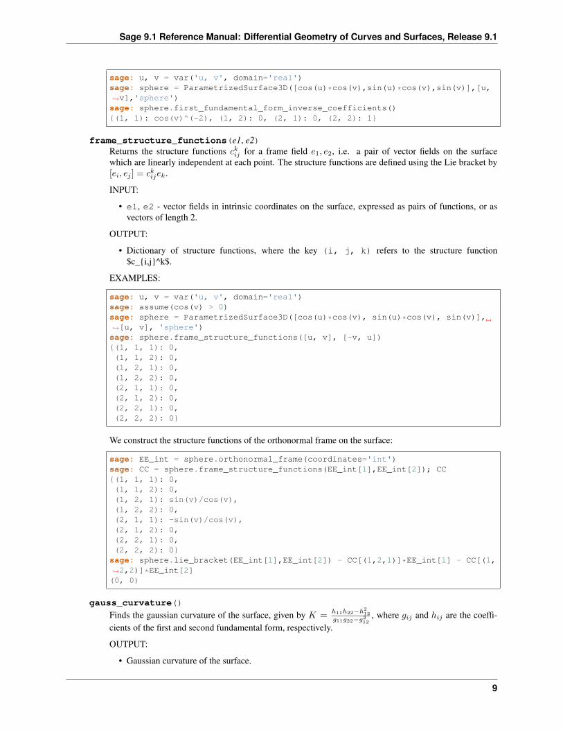
frame_structure_functions(e1, e2)Returns the structure functions 𝑐𝑘𝑖𝑗 for a frame field 𝑒1, 𝑒2, i.e. a pair of vector fields on the surfacewhich are linearly independent at each point. The structure functions are defined using the Lie bracket by[𝑒𝑖, 𝑒𝑗 ] = 𝑐𝑘𝑖𝑗𝑒𝑘.

INPUT:

• e1, e2 - vector fields in intrinsic coordinates on the surface, expressed as pairs of functions, or asvectors of length 2.

OUTPUT:

• Dictionary of structure functions, where the key (i, j, k) refers to the structure function$c_{i,j}^k$.

EXAMPLES:

sage: u, v = var('u, v', domain='real')sage: assume(cos(v) > 0)sage: sphere = ParametrizedSurface3D([cos(u)*cos(v), sin(u)*cos(v), sin(v)],→˓[u, v], 'sphere')sage: sphere.frame_structure_functions([u, v], [-v, u]){(1, 1, 1): 0,(1, 1, 2): 0,(1, 2, 1): 0,(1, 2, 2): 0,(2, 1, 1): 0,(2, 1, 2): 0,(2, 2, 1): 0,(2, 2, 2): 0}

We construct the structure functions of the orthonormal frame on the surface:

sage: EE_int = sphere.orthonormal_frame(coordinates='int')sage: CC = sphere.frame_structure_functions(EE_int[1],EE_int[2]); CC{(1, 1, 1): 0,(1, 1, 2): 0,(1, 2, 1): sin(v)/cos(v),(1, 2, 2): 0,(2, 1, 1): -sin(v)/cos(v),(2, 1, 2): 0,(2, 2, 1): 0,(2, 2, 2): 0}

sage: sphere.lie_bracket(EE_int[1],EE_int[2]) - CC[(1,2,1)]*EE_int[1] - CC[(1,→˓2,2)]*EE_int[2](0, 0)

gauss_curvature()Finds the gaussian curvature of the surface, given by 𝐾 =

ℎ11ℎ22−ℎ212

𝑔11𝑔22−𝑔212

, where 𝑔𝑖𝑗 and ℎ𝑖𝑗 are the coeffi-cients of the first and second fundamental form, respectively.

OUTPUT:

• Gaussian curvature of the surface.

9


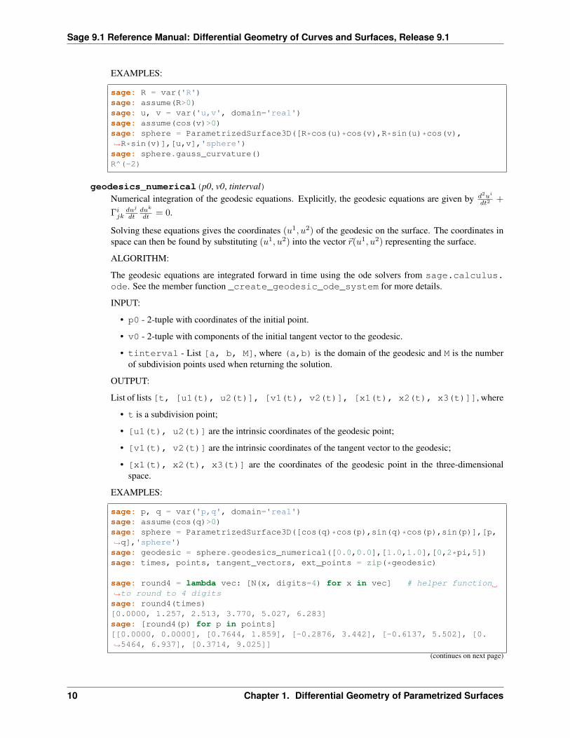
EXAMPLES:

sage: R = var('R')sage: assume(R>0)sage: u, v = var('u,v', domain='real')sage: assume(cos(v)>0)sage: sphere = ParametrizedSurface3D([R*cos(u)*cos(v),R*sin(u)*cos(v),→˓R*sin(v)],[u,v],'sphere')sage: sphere.gauss_curvature()R^(-2)

geodesics_numerical(p0, v0, tinterval)Numerical integration of the geodesic equations. Explicitly, the geodesic equations are given by 𝑑2𝑢𝑖

𝑑𝑡2 +

Γ𝑖𝑗𝑘

𝑑𝑢𝑗

𝑑𝑡𝑑𝑢𝑘

𝑑𝑡 = 0.

Solving these equations gives the coordinates (𝑢1, 𝑢2) of the geodesic on the surface. The coordinates inspace can then be found by substituting (𝑢1, 𝑢2) into the vector �⃗�(𝑢1, 𝑢2) representing the surface.

ALGORITHM:

The geodesic equations are integrated forward in time using the ode solvers from sage.calculus.ode. See the member function _create_geodesic_ode_system for more details.

INPUT:

• p0 - 2-tuple with coordinates of the initial point.

• v0 - 2-tuple with components of the initial tangent vector to the geodesic.

• tinterval - List [a, b, M], where (a,b) is the domain of the geodesic and M is the numberof subdivision points used when returning the solution.

OUTPUT:

List of lists [t, [u1(t), u2(t)], [v1(t), v2(t)], [x1(t), x2(t), x3(t)]], where

• t is a subdivision point;

• [u1(t), u2(t)] are the intrinsic coordinates of the geodesic point;

• [v1(t), v2(t)] are the intrinsic coordinates of the tangent vector to the geodesic;

• [x1(t), x2(t), x3(t)] are the coordinates of the geodesic point in the three-dimensionalspace.

EXAMPLES:

sage: p, q = var('p,q', domain='real')sage: assume(cos(q)>0)sage: sphere = ParametrizedSurface3D([cos(q)*cos(p),sin(q)*cos(p),sin(p)],[p,→˓q],'sphere')sage: geodesic = sphere.geodesics_numerical([0.0,0.0],[1.0,1.0],[0,2*pi,5])sage: times, points, tangent_vectors, ext_points = zip(*geodesic)

sage: round4 = lambda vec: [N(x, digits=4) for x in vec] # helper function→˓to round to 4 digitssage: round4(times)[0.0000, 1.257, 2.513, 3.770, 5.027, 6.283]sage: [round4(p) for p in points][[0.0000, 0.0000], [0.7644, 1.859], [-0.2876, 3.442], [-0.6137, 5.502], [0.→˓5464, 6.937], [0.3714, 9.025]]





sage: [round4(p) for p in ext_points][[1.000, 0.0000, 0.0000], [-0.2049, 0.6921, 0.6921], [-0.9160, -0.2836, -0.→˓2836], [0.5803, -0.5759, -0.5759], [0.6782, 0.5196, 0.5196], [-0.8582, 0.→˓3629, 0.3629]]

lie_bracket(v, w)Returns the Lie bracket of two vector fields that are tangent to the surface. The vector fields should begiven in intrinsic coordinates, i.e. with respect to the natural frame.

INPUT:

• v and w - vector fields on the surface, expressed as pairs of functions or as vectors of length 2.

OUTPUT:

• The Lie bracket $[v, w]$.

EXAMPLES:

sage: u, v = var('u, v', domain='real')sage: assume(cos(v)>0)sage: sphere = ParametrizedSurface3D([cos(u)*cos(v),sin(u)*cos(v),sin(v)],[u,→˓v],'sphere')sage: sphere.lie_bracket([u,v],[-v,u])(0, 0)

sage: EE_int = sphere.orthonormal_frame(coordinates='int')sage: sphere.lie_bracket(EE_int[1],EE_int[2])(sin(v)/cos(v)^2, 0)

mean_curvature()Finds the mean curvature of the surface, given by 𝐻 = 1

2𝑔22ℎ11−2𝑔12ℎ12+𝑔11ℎ22

𝑔11𝑔22−𝑔212

, where 𝑔𝑖𝑗 and ℎ𝑖𝑗 are thecomponents of the first and second fundamental forms, respectively.

OUTPUT:

• Mean curvature of the surface

EXAMPLES:

sage: R = var('R')sage: assume(R>0)sage: u, v = var('u,v', domain='real')sage: assume(cos(v)>0)sage: sphere = ParametrizedSurface3D([R*cos(u)*cos(v),R*sin(u)*cos(v),→˓R*sin(v)],[u,v],'sphere')sage: sphere.mean_curvature()-1/R

natural_frame()Returns the natural tangent frame on the parametrized surface. The vectors of this frame are tangent to thecoordinate lines on the surface.

OUTPUT:

• The natural frame as a dictionary.

EXAMPLES:

11


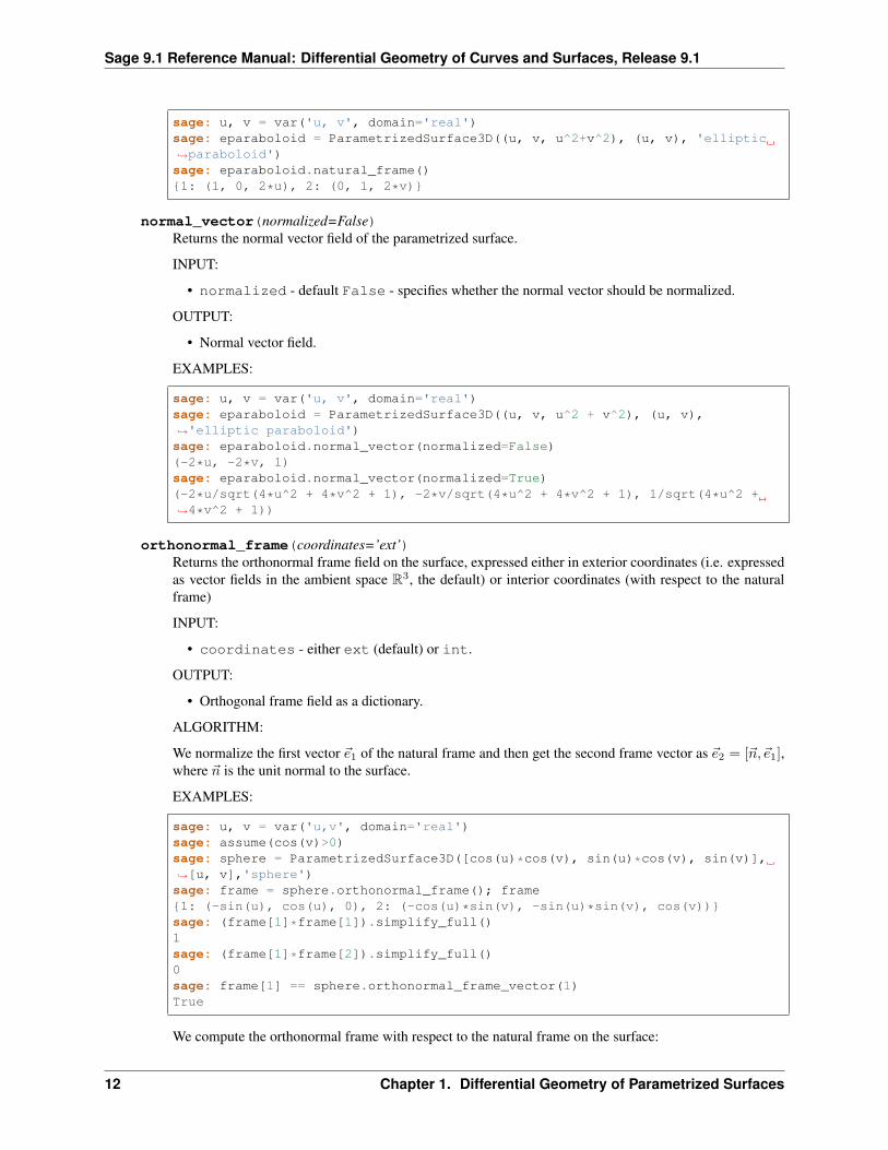
sage: u, v = var('u, v', domain='real')sage: eparaboloid = ParametrizedSurface3D((u, v, u^2+v^2), (u, v), 'elliptic→˓paraboloid')sage: eparaboloid.natural_frame(){1: (1, 0, 2*u), 2: (0, 1, 2*v)}

normal_vector(normalized=False)Returns the normal vector field of the parametrized surface.

INPUT:

• normalized - default False - specifies whether the normal vector should be normalized.

OUTPUT:

• Normal vector field.

EXAMPLES:

sage: u, v = var('u, v', domain='real')sage: eparaboloid = ParametrizedSurface3D((u, v, u^2 + v^2), (u, v),→˓'elliptic paraboloid')sage: eparaboloid.normal_vector(normalized=False)(-2*u, -2*v, 1)sage: eparaboloid.normal_vector(normalized=True)(-2*u/sqrt(4*u^2 + 4*v^2 + 1), -2*v/sqrt(4*u^2 + 4*v^2 + 1), 1/sqrt(4*u^2 +→˓4*v^2 + 1))

orthonormal_frame(coordinates=’ext’)Returns the orthonormal frame field on the surface, expressed either in exterior coordinates (i.e. expressedas vector fields in the ambient space R3, the default) or interior coordinates (with respect to the naturalframe)

INPUT:

• coordinates - either ext (default) or int.

OUTPUT:

• Orthogonal frame field as a dictionary.

ALGORITHM:

We normalize the first vector �⃗�1 of the natural frame and then get the second frame vector as �⃗�2 = [�⃗�, �⃗�1],where �⃗� is the unit normal to the surface.

EXAMPLES:

sage: u, v = var('u,v', domain='real')sage: assume(cos(v)>0)sage: sphere = ParametrizedSurface3D([cos(u)*cos(v), sin(u)*cos(v), sin(v)],→˓[u, v],'sphere')sage: frame = sphere.orthonormal_frame(); frame{1: (-sin(u), cos(u), 0), 2: (-cos(u)*sin(v), -sin(u)*sin(v), cos(v))}sage: (frame[1]*frame[1]).simplify_full()1sage: (frame[1]*frame[2]).simplify_full()0sage: frame[1] == sphere.orthonormal_frame_vector(1)True

We compute the orthonormal frame with respect to the natural frame on the surface:



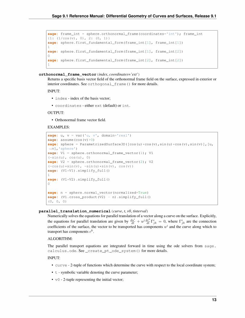
sage: frame_int = sphere.orthonormal_frame(coordinates='int'); frame_int{1: (1/cos(v), 0), 2: (0, 1)}sage: sphere.first_fundamental_form(frame_int[1], frame_int[1])1sage: sphere.first_fundamental_form(frame_int[1], frame_int[2])0sage: sphere.first_fundamental_form(frame_int[2], frame_int[2])1

orthonormal_frame_vector(index, coordinates=’ext’)Returns a specific basis vector field of the orthonormal frame field on the surface, expressed in exterior orinterior coordinates. See orthogonal_frame() for more details.

INPUT:

• index - index of the basis vector;

• coordinates - either ext (default) or int.

OUTPUT:

• Orthonormal frame vector field.

EXAMPLES:

sage: u, v = var('u, v', domain='real')sage: assume(cos(v)>0)sage: sphere = ParametrizedSurface3D([cos(u)*cos(v),sin(u)*cos(v),sin(v)],[u,→˓v],'sphere')sage: V1 = sphere.orthonormal_frame_vector(1); V1(-sin(u), cos(u), 0)sage: V2 = sphere.orthonormal_frame_vector(2); V2(-cos(u)*sin(v), -sin(u)*sin(v), cos(v))sage: (V1*V1).simplify_full()1sage: (V1*V2).simplify_full()0

sage: n = sphere.normal_vector(normalized=True)sage: (V1.cross_product(V2) - n).simplify_full()(0, 0, 0)

parallel_translation_numerical(curve, t, v0, tinterval)Numerically solves the equations for parallel translation of a vector along a curve on the surface. Explicitly,the equations for parallel translation are given by 𝑑𝑢𝑖

𝑑𝑡 + 𝑢𝑗 𝑑𝑐𝑘

𝑑𝑡 Γ𝑖𝑗𝑘 = 0, where Γ𝑖

𝑗𝑘 are the connectioncoefficients of the surface, the vector to be transported has components 𝑢𝑗 and the curve along which totransport has components 𝑐𝑘.

ALGORITHM:

The parallel transport equations are integrated forward in time using the ode solvers from sage.calculus.ode. See _create_pt_ode_system() for more details.

INPUT:

• curve - 2-tuple of functions which determine the curve with respect to the local coordinate system;

• t - symbolic variable denoting the curve parameter;

• v0 - 2-tuple representing the initial vector;

13


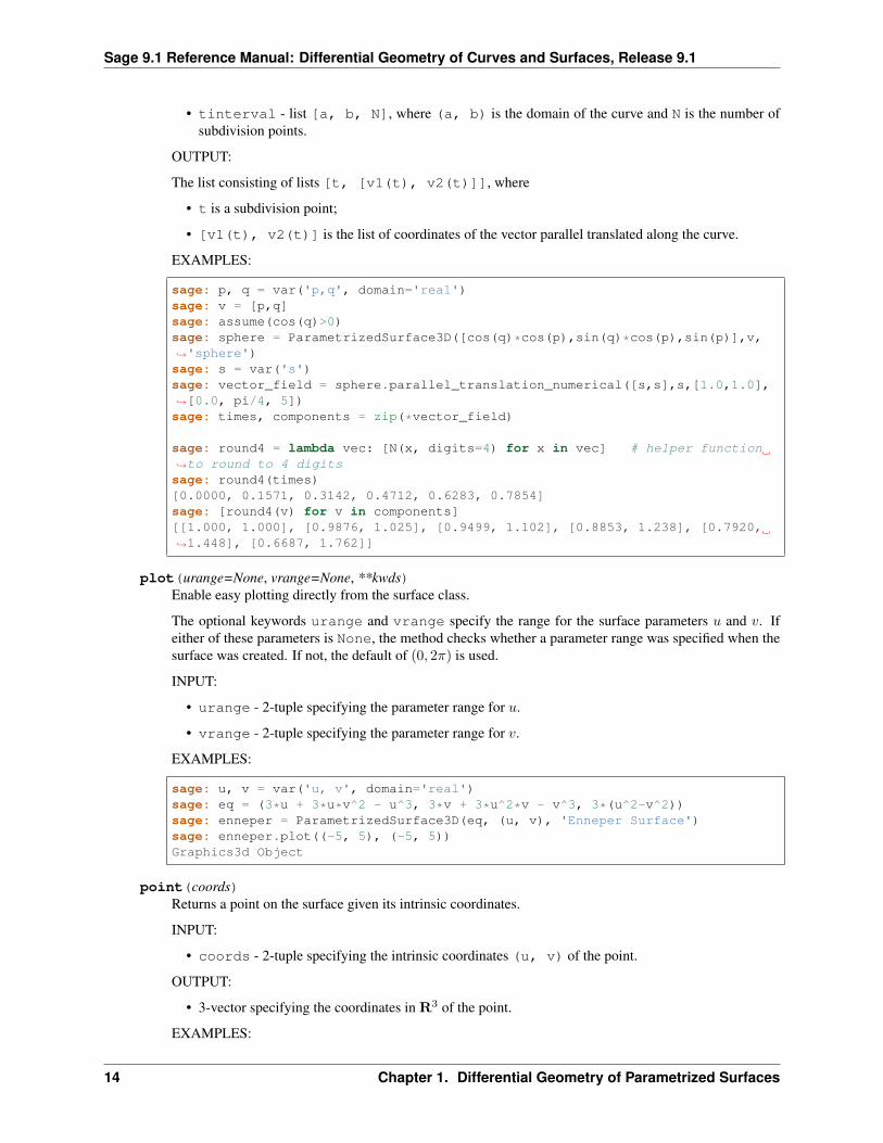
• tinterval - list [a, b, N], where (a, b) is the domain of the curve and N is the number ofsubdivision points.

OUTPUT:

The list consisting of lists [t, [v1(t), v2(t)]], where

• t is a subdivision point;

• [v1(t), v2(t)] is the list of coordinates of the vector parallel translated along the curve.

EXAMPLES:

sage: p, q = var('p,q', domain='real')sage: v = [p,q]sage: assume(cos(q)>0)sage: sphere = ParametrizedSurface3D([cos(q)*cos(p),sin(q)*cos(p),sin(p)],v,→˓'sphere')sage: s = var('s')sage: vector_field = sphere.parallel_translation_numerical([s,s],s,[1.0,1.0],→˓[0.0, pi/4, 5])sage: times, components = zip(*vector_field)

sage: round4 = lambda vec: [N(x, digits=4) for x in vec] # helper function→˓to round to 4 digitssage: round4(times)[0.0000, 0.1571, 0.3142, 0.4712, 0.6283, 0.7854]sage: [round4(v) for v in components][[1.000, 1.000], [0.9876, 1.025], [0.9499, 1.102], [0.8853, 1.238], [0.7920,→˓1.448], [0.6687, 1.762]]

plot(urange=None, vrange=None, **kwds)Enable easy plotting directly from the surface class.

The optional keywords urange and vrange specify the range for the surface parameters 𝑢 and 𝑣. Ifeither of these parameters is None, the method checks whether a parameter range was specified when thesurface was created. If not, the default of (0, 2𝜋) is used.

INPUT:

• urange - 2-tuple specifying the parameter range for 𝑢.

• vrange - 2-tuple specifying the parameter range for 𝑣.

EXAMPLES:

sage: u, v = var('u, v', domain='real')sage: eq = (3*u + 3*u*v^2 - u^3, 3*v + 3*u^2*v - v^3, 3*(u^2-v^2))sage: enneper = ParametrizedSurface3D(eq, (u, v), 'Enneper Surface')sage: enneper.plot((-5, 5), (-5, 5))Graphics3d Object

point(coords)Returns a point on the surface given its intrinsic coordinates.

INPUT:

• coords - 2-tuple specifying the intrinsic coordinates (u, v) of the point.

OUTPUT:

• 3-vector specifying the coordinates in R3 of the point.

EXAMPLES:



sage: u, v = var('u, v', domain='real')sage: torus = ParametrizedSurface3D(((2 + cos(u))*cos(v),(2 + cos(u))*sin(v),→˓sin(u)),[u,v],'torus')sage: torus.point((0, pi/2))(0, 3, 0)sage: torus.point((pi/2, pi))(-2, 0, 1)sage: torus.point((pi, pi/2))(0, 1, 0)

principal_directions()Finds the principal curvatures and principal directions of the surface

OUTPUT:

For each principal curvature, returns a list of the form (𝜌, 𝑉, 𝑛), where 𝜌 is the principal curvature, 𝑉 isthe corresponding principal direction, and 𝑛 is the multiplicity.

EXAMPLES:

sage: u, v = var('u, v', domain='real')sage: R, r = var('R,r', domain='real')sage: assume(R>r,r>0)sage: torus = ParametrizedSurface3D([(R+r*cos(v))*cos(u),(R+r*cos(v))*sin(u),→˓r*sin(v)],[u,v],'torus')sage: torus.principal_directions()[(-cos(v)/(r*cos(v) + R), [(1, 0)], 1), (-1/r, [(0, 1)], 1)]

sage: u, v = var('u, v', domain='real')sage: V = vector([u*cos(u+v), u*sin(u+v), u+v])sage: helicoid = ParametrizedSurface3D(V, (u, v))sage: helicoid.principal_directions()[(-1/(u^2 + 1), [(1, -(u^2 - sqrt(u^2 + 1) + 1)/(u^2 + 1))], 1),(1/(u^2 + 1), [(1, -(u^2 + sqrt(u^2 + 1) + 1)/(u^2 + 1))], 1)]

rotation(theta)Gives the matrix of the rotation operator over a given angle 𝜃 with respect to the natural frame.

INPUT:

• theta - rotation angle

OUTPUT:

• Rotation matrix with respect to the natural frame.

ALGORITHM:

The operator of rotation over 𝜋/2 is 𝐽 𝑖𝑗 = 𝑔𝑖𝑘𝜔𝑗𝑘, where 𝜔 is the area form. The operator of rotation over

an angle 𝜃 is cos(𝜃)𝐼 + 𝑠𝑖𝑛(𝜃)𝐽 .

EXAMPLES:

sage: u, v = var('u, v', domain='real')sage: assume(cos(v)>0)sage: sphere = ParametrizedSurface3D([cos(u)*cos(v),sin(u)*cos(v),sin(v)],[u,→˓v],'sphere')

We first compute the matrix of rotation over 𝜋/3:

15


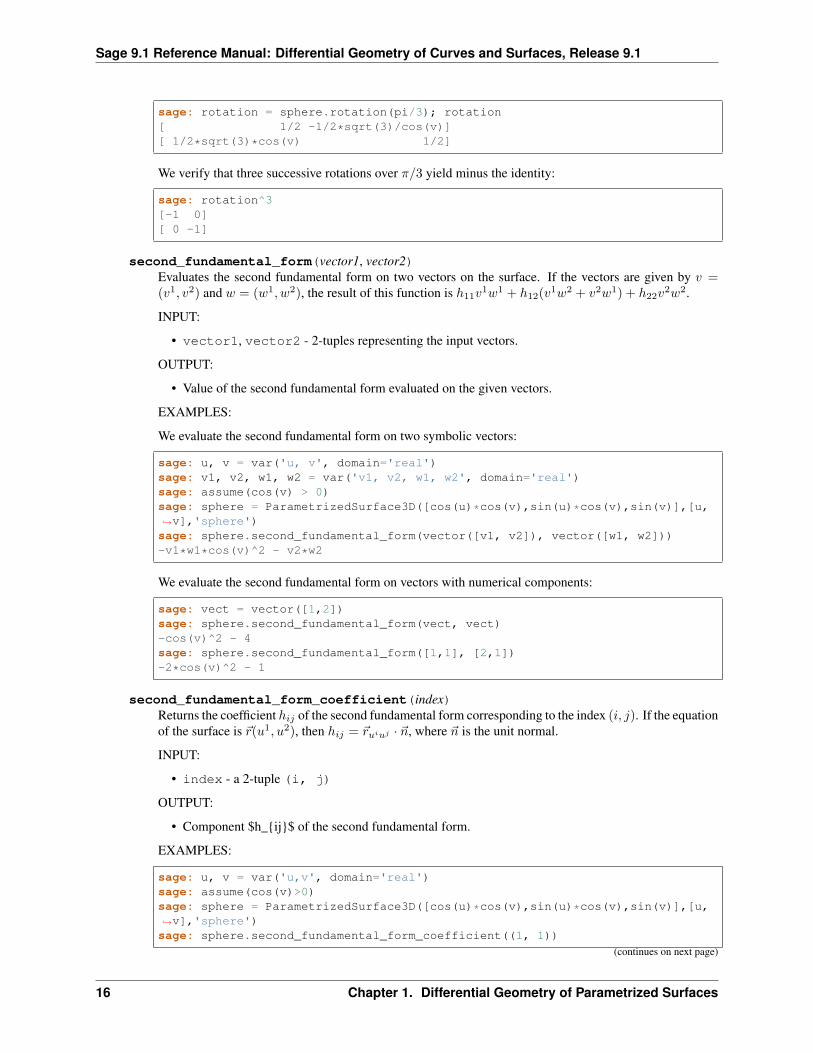
sage: rotation = sphere.rotation(pi/3); rotation[ 1/2 -1/2*sqrt(3)/cos(v)][ 1/2*sqrt(3)*cos(v) 1/2]

We verify that three successive rotations over 𝜋/3 yield minus the identity:

sage: rotation^3[-1 0][ 0 -1]

second_fundamental_form(vector1, vector2)Evaluates the second fundamental form on two vectors on the surface. If the vectors are given by 𝑣 =(𝑣1, 𝑣2) and 𝑤 = (𝑤1, 𝑤2), the result of this function is ℎ11𝑣

1𝑤1 + ℎ12(𝑣1𝑤2 + 𝑣2𝑤1) + ℎ22𝑣2𝑤2.

INPUT:

• vector1, vector2 - 2-tuples representing the input vectors.

OUTPUT:

• Value of the second fundamental form evaluated on the given vectors.

EXAMPLES:

We evaluate the second fundamental form on two symbolic vectors:

sage: u, v = var('u, v', domain='real')sage: v1, v2, w1, w2 = var('v1, v2, w1, w2', domain='real')sage: assume(cos(v) > 0)sage: sphere = ParametrizedSurface3D([cos(u)*cos(v),sin(u)*cos(v),sin(v)],[u,→˓v],'sphere')sage: sphere.second_fundamental_form(vector([v1, v2]), vector([w1, w2]))-v1*w1*cos(v)^2 - v2*w2

We evaluate the second fundamental form on vectors with numerical components:

sage: vect = vector([1,2])sage: sphere.second_fundamental_form(vect, vect)-cos(v)^2 - 4sage: sphere.second_fundamental_form([1,1], [2,1])-2*cos(v)^2 - 1

second_fundamental_form_coefficient(index)Returns the coefficient ℎ𝑖𝑗 of the second fundamental form corresponding to the index (𝑖, 𝑗). If the equationof the surface is �⃗�(𝑢1, 𝑢2), then ℎ𝑖𝑗 = �⃗�𝑢𝑖𝑢𝑗 · �⃗�, where �⃗� is the unit normal.

INPUT:

• index - a 2-tuple (i, j)

OUTPUT:

• Component $h_{ij}$ of the second fundamental form.

EXAMPLES:

sage: u, v = var('u,v', domain='real')sage: assume(cos(v)>0)sage: sphere = ParametrizedSurface3D([cos(u)*cos(v),sin(u)*cos(v),sin(v)],[u,→˓v],'sphere')sage: sphere.second_fundamental_form_coefficient((1, 1))





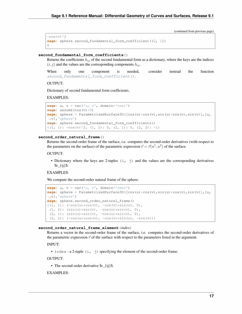
-cos(v)^2sage: sphere.second_fundamental_form_coefficient((2, 1))0

second_fundamental_form_coefficients()Returns the coefficients ℎ𝑖𝑗 of the second fundamental form as a dictionary, where the keys are the indices(𝑖, 𝑗) and the values are the corresponding components ℎ𝑖𝑗 .

When only one component is needed, consider instead the functionsecond_fundamental_form_coefficient().

OUTPUT:

Dictionary of second fundamental form coefficients.

EXAMPLES:

sage: u, v = var('u, v', domain='real')sage: assume(cos(v)>0)sage: sphere = ParametrizedSurface3D([cos(u)*cos(v),sin(u)*cos(v),sin(v)],[u,→˓v],'sphere')sage: sphere.second_fundamental_form_coefficients(){(1, 1): -cos(v)^2, (1, 2): 0, (2, 1): 0, (2, 2): -1}

second_order_natural_frame()Returns the second-order frame of the surface, i.e. computes the second-order derivatives (with respect tothe parameters on the surface) of the parametric expression �⃗� = �⃗�(𝑢1, 𝑢2) of the surface.

OUTPUT:

• Dictionary where the keys are 2-tuples (i, j) and the values are the corresponding derivatives$r_{ij}$.

EXAMPLES:

We compute the second-order natural frame of the sphere:

sage: u, v = var('u, v', domain='real')sage: sphere = ParametrizedSurface3D([cos(u)*cos(v),sin(u)*cos(v),sin(v)],[u,→˓v],'sphere')sage: sphere.second_order_natural_frame(){(1, 1): (-cos(u)*cos(v), -cos(v)*sin(u), 0),(1, 2): (sin(u)*sin(v), -cos(u)*sin(v), 0),(2, 1): (sin(u)*sin(v), -cos(u)*sin(v), 0),(2, 2): (-cos(u)*cos(v), -cos(v)*sin(u), -sin(v))}

second_order_natural_frame_element(index)Returns a vector in the second-order frame of the surface, i.e. computes the second-order derivatives ofthe parametric expression �⃗� of the surface with respect to the parameters listed in the argument.

INPUT:

• index - a 2-tuple (i, j) specifying the element of the second-order frame.

OUTPUT:

• The second-order derivative $r_{ij}$.

EXAMPLES:

17


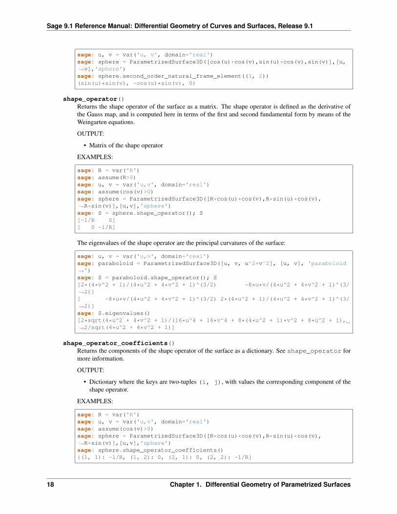
sage: u, v = var('u, v', domain='real')sage: sphere = ParametrizedSurface3D([cos(u)*cos(v),sin(u)*cos(v),sin(v)],[u,→˓v],'sphere')sage: sphere.second_order_natural_frame_element((1, 2))(sin(u)*sin(v), -cos(u)*sin(v), 0)

shape_operator()Returns the shape operator of the surface as a matrix. The shape operator is defined as the derivative ofthe Gauss map, and is computed here in terms of the first and second fundamental form by means of theWeingarten equations.

OUTPUT:

• Matrix of the shape operator

EXAMPLES:

sage: R = var('R')sage: assume(R>0)sage: u, v = var('u,v', domain='real')sage: assume(cos(v)>0)sage: sphere = ParametrizedSurface3D([R*cos(u)*cos(v),R*sin(u)*cos(v),→˓R*sin(v)],[u,v],'sphere')sage: S = sphere.shape_operator(); S[-1/R 0][ 0 -1/R]

The eigenvalues of the shape operator are the principal curvatures of the surface:

sage: u, v = var('u,v', domain='real')sage: paraboloid = ParametrizedSurface3D([u, v, u^2+v^2], [u, v], 'paraboloid→˓')sage: S = paraboloid.shape_operator(); S[2*(4*v^2 + 1)/(4*u^2 + 4*v^2 + 1)^(3/2) -8*u*v/(4*u^2 + 4*v^2 + 1)^(3/→˓2)][ -8*u*v/(4*u^2 + 4*v^2 + 1)^(3/2) 2*(4*u^2 + 1)/(4*u^2 + 4*v^2 + 1)^(3/→˓2)]sage: S.eigenvalues()[2*sqrt(4*u^2 + 4*v^2 + 1)/(16*u^4 + 16*v^4 + 8*(4*u^2 + 1)*v^2 + 8*u^2 + 1),→˓2/sqrt(4*u^2 + 4*v^2 + 1)]

shape_operator_coefficients()Returns the components of the shape operator of the surface as a dictionary. See shape_operator formore information.

OUTPUT:

• Dictionary where the keys are two-tuples (i, j), with values the corresponding component of theshape operator.

EXAMPLES:

sage: R = var('R')sage: u, v = var('u,v', domain='real')sage: assume(cos(v)>0)sage: sphere = ParametrizedSurface3D([R*cos(u)*cos(v),R*sin(u)*cos(v),→˓R*sin(v)],[u,v],'sphere')sage: sphere.shape_operator_coefficients(){(1, 1): -1/R, (1, 2): 0, (2, 1): 0, (2, 2): -1/R}



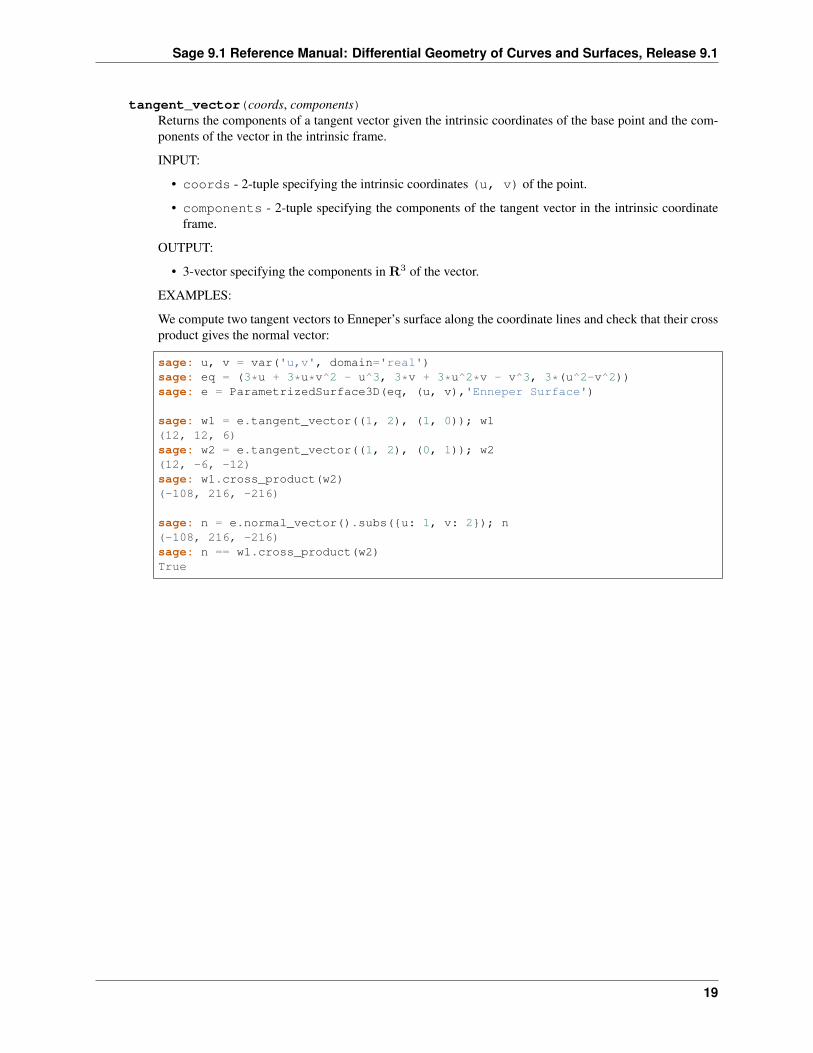
tangent_vector(coords, components)Returns the components of a tangent vector given the intrinsic coordinates of the base point and the com-ponents of the vector in the intrinsic frame.

INPUT:

• coords - 2-tuple specifying the intrinsic coordinates (u, v) of the point.

• components - 2-tuple specifying the components of the tangent vector in the intrinsic coordinateframe.

OUTPUT:

• 3-vector specifying the components in R3 of the vector.

EXAMPLES:

We compute two tangent vectors to Enneper’s surface along the coordinate lines and check that their crossproduct gives the normal vector:

sage: u, v = var('u,v', domain='real')sage: eq = (3*u + 3*u*v^2 - u^3, 3*v + 3*u^2*v - v^3, 3*(u^2-v^2))sage: e = ParametrizedSurface3D(eq, (u, v),'Enneper Surface')

sage: w1 = e.tangent_vector((1, 2), (1, 0)); w1(12, 12, 6)sage: w2 = e.tangent_vector((1, 2), (0, 1)); w2(12, -6, -12)sage: w1.cross_product(w2)(-108, 216, -216)

sage: n = e.normal_vector().subs({u: 1, v: 2}); n(-108, 216, -216)sage: n == w1.cross_product(w2)True

19



CHAPTER

TWO

COMMON PARAMETRIZED SURFACES IN 3D.

AUTHORS:

- Joris Vankerschaver (2012-06-16)

class sage.geometry.riemannian_manifolds.surface3d_generators.SurfaceGeneratorsBases: object

A class consisting of generators for several common parametrized surfaces in 3D.

static Catenoid(c=1, name=’Catenoid’)Return a catenoid surface, with parametric representation

𝑥(𝑢, 𝑣) = 𝑐 cosh(𝑣/𝑐) cos(𝑢);

𝑦(𝑢, 𝑣) = 𝑐 cosh(𝑣/𝑐) sin(𝑢);

𝑧(𝑢, 𝑣) = 𝑣.

INPUT:

• c – surface parameter.

• name – string. Name of the surface.

For more information, see Wikipedia article Catenoid.

EXAMPLES:

sage: cat = surfaces.Catenoid(); catParametrized surface ('Catenoid') with equation (cos(u)*cosh(v),→˓cosh(v)*sin(u), v)sage: cat.plot()Graphics3d Object

static Crosscap(r=1, name=’Crosscap’)Return a crosscap surface, with parametrization

𝑥(𝑢, 𝑣) = 𝑟(1 + cos(𝑣)) cos(𝑢);

𝑦(𝑢, 𝑣) = 𝑟(1 + cos(𝑣)) sin(𝑢);

𝑧(𝑢, 𝑣) = −𝑟 tanh(𝑢− 𝜋) sin(𝑣).

INPUT:

• r – surface parameter.


For more information, see Wikipedia article Cross-cap.

EXAMPLES:

21

https://en.wikipedia.org/wiki/Catenoid

https://en.wikipedia.org/wiki/Cross-cap


sage: crosscap = surfaces.Crosscap(); crosscapParametrized surface ('Crosscap') with equation ((cos(v) + 1)*cos(u), (cos(v)→˓+ 1)*sin(u), -sin(v)*tanh(-pi + u))sage: crosscap.plot()Graphics3d Object

static Dini(a=1, b=1, name="Dini’s surface")Return Dini’s surface, with parametrization

𝑥(𝑢, 𝑣) = 𝑎 cos(𝑢) sin(𝑣);

𝑦(𝑢, 𝑣) = 𝑎 sin(𝑢) sin(𝑣);

𝑧(𝑢, 𝑣) = 𝑢 + log(tan(𝑣/2)) + cos(𝑣).

INPUT:

• a, b – surface parameters.


For more information, see Wikipedia article Dini’s_surface.

EXAMPLES:

sage: dini = surfaces.Dini(a=3, b=4); diniParametrized surface ('Dini's surface') with equation (3*cos(u)*sin(v),→˓3*sin(u)*sin(v), 4*u + 3*cos(v) + 3*log(tan(1/2*v)))sage: dini.plot()Graphics3d Object

static Ellipsoid(center=(0, 0, 0), axes=(1, 1, 1), name=’Ellipsoid’)Return an ellipsoid centered at center whose semi-principal axes have lengths given by the componentsof axes. The parametrization of the ellipsoid is given by

𝑥(𝑢, 𝑣) = 𝑥0 + 𝑎 cos(𝑢) cos(𝑣);

𝑦(𝑢, 𝑣) = 𝑦0 + 𝑏 sin(𝑢) cos(𝑣);

𝑧(𝑢, 𝑣) = 𝑧0 + 𝑐 sin(𝑣).

INPUT:

• center – 3-tuple. Coordinates of the center of the ellipsoid.

• axes – 3-tuple. Lengths of the semi-principal axes.

• name – string. Name of the ellipsoid.

For more information, see Wikipedia article Ellipsoid.

EXAMPLES:

sage: ell = surfaces.Ellipsoid(axes=(1, 2, 3)); ellParametrized surface ('Ellipsoid') with equation (cos(u)*cos(v),→˓2*cos(v)*sin(u), 3*sin(v))sage: ell.plot()Graphics3d Object

static Enneper(name="Enneper’s surface")Return Enneper’s surface, with parametrization

𝑥(𝑢, 𝑣) = 𝑢(1 − 𝑢2/3 + 𝑣2)/3;

𝑦(𝑢, 𝑣) = −𝑣(1 − 𝑣2/3 + 𝑢2)/3;

𝑧(𝑢, 𝑣) = (𝑢2 − 𝑣2)/3.

22 Chapter 2. Common parametrized surfaces in 3D.

https://en.wikipedia.org/wiki/Dini's_surface

https://en.wikipedia.org/wiki/Ellipsoid


INPUT:


For more information, see Wikipedia article Enneper_surface.

EXAMPLES:

sage: enn = surfaces.Enneper(); ennParametrized surface ('Enneper's surface') with equation (-1/9*(u^2 - 3*v^2 -→˓3)*u, -1/9*(3*u^2 - v^2 + 3)*v, 1/3*u^2 - 1/3*v^2)sage: enn.plot()Graphics3d Object

static Helicoid(h=1, name=’Helicoid’)Return a helicoid surface, with parametrization

𝑥(𝜌, 𝜃) = 𝜌 cos(𝜃);

𝑦(𝜌, 𝜃) = 𝜌 sin(𝜃);

𝑧(𝜌, 𝜃) = ℎ𝜃/(2𝜋).

INPUT:

• h – distance along the z-axis between two successive turns of the helicoid.


For more information, see Wikipedia article Helicoid.

EXAMPLES:

sage: helicoid = surfaces.Helicoid(h=2); helicoidParametrized surface ('Helicoid') with equation (rho*cos(theta),→˓rho*sin(theta), theta/pi)sage: helicoid.plot()Graphics3d Object

static Klein(r=1, name=’Klein bottle’)Return the Klein bottle, in the figure-8 parametrization given by

𝑥(𝑢, 𝑣) = (𝑟 + cos(𝑢/2) cos(𝑣) − sin(𝑢/2) sin(2𝑣)) cos(𝑢);

𝑦(𝑢, 𝑣) = (𝑟 + cos(𝑢/2) cos(𝑣) − sin(𝑢/2) sin(2𝑣)) sin(𝑢);

𝑧(𝑢, 𝑣) = sin(𝑢/2) cos(𝑣) + cos(𝑢/2) sin(2𝑣).

INPUT:

• r – radius of the “figure-8” circle.


For more information, see Wikipedia article Klein_bottle.

EXAMPLES:

sage: klein = surfaces.Klein(); kleinParametrized surface ('Klein bottle') with equation (-(sin(1/2*u)*sin(2*v) -→˓cos(1/2*u)*sin(v) - 1)*cos(u), -(sin(1/2*u)*sin(2*v) - cos(1/2*u)*sin(v) -→˓1)*sin(u), cos(1/2*u)*sin(2*v) + sin(1/2*u)*sin(v))sage: klein.plot()Graphics3d Object

23

https://en.wikipedia.org/wiki/Enneper_surface

https://en.wikipedia.org/wiki/Helicoid

https://en.wikipedia.org/wiki/Klein_bottle


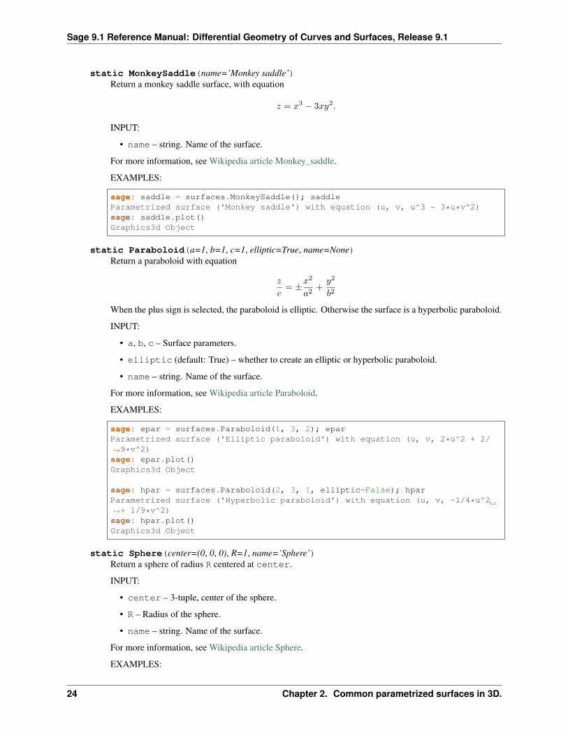
static MonkeySaddle(name=’Monkey saddle’)Return a monkey saddle surface, with equation

𝑧 = 𝑥3 − 3𝑥𝑦2.

INPUT:


For more information, see Wikipedia article Monkey_saddle.

EXAMPLES:

sage: saddle = surfaces.MonkeySaddle(); saddleParametrized surface ('Monkey saddle') with equation (u, v, u^3 - 3*u*v^2)sage: saddle.plot()Graphics3d Object

static Paraboloid(a=1, b=1, c=1, elliptic=True, name=None)Return a paraboloid with equation

𝑧

𝑐= ±𝑥2

𝑎2+

𝑦2

𝑏2

When the plus sign is selected, the paraboloid is elliptic. Otherwise the surface is a hyperbolic paraboloid.

INPUT:

• a, b, c – Surface parameters.

• elliptic (default: True) – whether to create an elliptic or hyperbolic paraboloid.


For more information, see Wikipedia article Paraboloid.

EXAMPLES:

sage: epar = surfaces.Paraboloid(1, 3, 2); eparParametrized surface ('Elliptic paraboloid') with equation (u, v, 2*u^2 + 2/→˓9*v^2)sage: epar.plot()Graphics3d Object

sage: hpar = surfaces.Paraboloid(2, 3, 1, elliptic=False); hparParametrized surface ('Hyperbolic paraboloid') with equation (u, v, -1/4*u^2→˓+ 1/9*v^2)sage: hpar.plot()Graphics3d Object

static Sphere(center=(0, 0, 0), R=1, name=’Sphere’)Return a sphere of radius R centered at center.

INPUT:

• center – 3-tuple, center of the sphere.

• R – Radius of the sphere.


For more information, see Wikipedia article Sphere.

EXAMPLES:


https://en.wikipedia.org/wiki/Monkey_saddle

https://en.wikipedia.org/wiki/Paraboloid

https://en.wikipedia.org/wiki/Sphere


sage: sphere = surfaces.Sphere(center=(0, 1, -1), R=2); sphereParametrized surface ('Sphere') with equation (2*cos(u)*cos(v),→˓2*cos(v)*sin(u) + 1, 2*sin(v) - 1)sage: sphere.plot()Graphics3d Object

Note that the radius of the sphere can be negative. The surface thus obtained is equal to the sphere (or partthereof) with positive radius, whose coordinate functions have been multiplied by -1. Compare for instantthe first octant of the unit sphere with positive radius:

sage: octant1 = surfaces.Sphere(R=1); octant1Parametrized surface ('Sphere') with equation (cos(u)*cos(v), cos(v)*sin(u),→˓sin(v))sage: octant1.plot((0, pi/2), (0, pi/2))Graphics3d Object

with the first octant of the unit sphere with negative radius:

sage: octant2 = surfaces.Sphere(R=-1); octant2Parametrized surface ('Sphere') with equation (-cos(u)*cos(v), -cos(v)*sin(u),→˓ -sin(v))sage: octant2.plot((0, pi/2), (0, pi/2))Graphics3d Object

static Torus(r=2, R=3, name=’Torus’)Return a torus obtained by revolving a circle of radius r around a coplanar axis R units away from thecenter of the circle. The parametrization used is

𝑥(𝑢, 𝑣) = (𝑅 + 𝑟 cos(𝑣)) cos(𝑢);

𝑦(𝑢, 𝑣) = (𝑅 + 𝑟 cos(𝑣)) sin(𝑢);

𝑧(𝑢, 𝑣) = 𝑟 sin(𝑣).

INPUT:

• r, R – Minor and major radius of the torus.


For more information, see Wikipedia article Torus.

EXAMPLES:

sage: torus = surfaces.Torus(); torusParametrized surface ('Torus') with equation ((2*cos(v) + 3)*cos(u),→˓(2*cos(v) + 3)*sin(u), 2*sin(v))sage: torus.plot()Graphics3d Object

static WhitneyUmbrella(name="Whitney’s umbrella")Return Whitney’s umbrella, with parametric representation

𝑥(𝑢, 𝑣) = 𝑢𝑣, 𝑦(𝑢, 𝑣) = 𝑢, 𝑧(𝑢, 𝑣) = 𝑣2.

INPUT:


For more information, see Wikipedia article Whitney_umbrella.

EXAMPLES:

25

https://en.wikipedia.org/wiki/Torus

https://en.wikipedia.org/wiki/Whitney_umbrella


sage: whitney = surfaces.WhitneyUmbrella(); whitneyParametrized surface ('Whitney's umbrella') with equation (u*v, u, v^2)sage: whitney.plot()Graphics3d Object


CHAPTER

THREE

INDICES AND TABLES

• Index

• Module Index

• Search Page

27

../genindex.html

../py-modindex.html

../search.html


28 Chapter 3. Indices and Tables

PYTHON MODULE INDEX

gsage.geometry.riemannian_manifolds.parametrized_surface3d, 1sage.geometry.riemannian_manifolds.surface3d_generators, 21

29


30 Python Module Index

INDEX

Aarea_form() (sage.geometry.riemannian_manifolds.parametrized_surface3d.ParametrizedSurface3D method), 6area_form_squared() (sage.geometry.riemannian_manifolds.parametrized_surface3d.ParametrizedSurface3D

method), 6

CCatenoid() (sage.geometry.riemannian_manifolds.surface3d_generators.SurfaceGenerators static method), 21connection_coefficients() (sage.geometry.riemannian_manifolds.parametrized_surface3d.ParametrizedSurface3D

method), 6Crosscap() (sage.geometry.riemannian_manifolds.surface3d_generators.SurfaceGenerators static method), 21

DDini() (sage.geometry.riemannian_manifolds.surface3d_generators.SurfaceGenerators static method), 22

EEllipsoid() (sage.geometry.riemannian_manifolds.surface3d_generators.SurfaceGenerators static method), 22Enneper() (sage.geometry.riemannian_manifolds.surface3d_generators.SurfaceGenerators static method), 22

Ffirst_fundamental_form() (sage.geometry.riemannian_manifolds.parametrized_surface3d.ParametrizedSurface3D

method), 7first_fundamental_form_coefficient() (sage.geometry.riemannian_manifolds.parametrized_surface3d.ParametrizedSurface3D

method), 7first_fundamental_form_coefficients() (sage.geometry.riemannian_manifolds.parametrized_surface3d.ParametrizedSurface3D

method), 8first_fundamental_form_inverse_coefficient() (sage.geometry.riemannian_manifolds.parametrized_surface3d.ParametrizedSurface3D

method), 8first_fundamental_form_inverse_coefficients() (sage.geometry.riemannian_manifolds.parametrized_surface3d.ParametrizedSurface3D

method), 8frame_structure_functions() (sage.geometry.riemannian_manifolds.parametrized_surface3d.ParametrizedSurface3D

method), 9

Ggauss_curvature() (sage.geometry.riemannian_manifolds.parametrized_surface3d.ParametrizedSurface3D

method), 9geodesics_numerical() (sage.geometry.riemannian_manifolds.parametrized_surface3d.ParametrizedSurface3D

method), 10

31


HHelicoid() (sage.geometry.riemannian_manifolds.surface3d_generators.SurfaceGenerators static method), 23

KKlein() (sage.geometry.riemannian_manifolds.surface3d_generators.SurfaceGenerators static method), 23

Llie_bracket() (sage.geometry.riemannian_manifolds.parametrized_surface3d.ParametrizedSurface3D method),

11

Mmean_curvature() (sage.geometry.riemannian_manifolds.parametrized_surface3d.ParametrizedSurface3D

method), 11MonkeySaddle() (sage.geometry.riemannian_manifolds.surface3d_generators.SurfaceGenerators static method),

23

Nnatural_frame() (sage.geometry.riemannian_manifolds.parametrized_surface3d.ParametrizedSurface3D

method), 11normal_vector() (sage.geometry.riemannian_manifolds.parametrized_surface3d.ParametrizedSurface3D

method), 12

Oorthonormal_frame() (sage.geometry.riemannian_manifolds.parametrized_surface3d.ParametrizedSurface3D

method), 12orthonormal_frame_vector() (sage.geometry.riemannian_manifolds.parametrized_surface3d.ParametrizedSurface3D

method), 13

PParaboloid() (sage.geometry.riemannian_manifolds.surface3d_generators.SurfaceGenerators static method), 24parallel_translation_numerical() (sage.geometry.riemannian_manifolds.parametrized_surface3d.ParametrizedSurface3D

method), 13ParametrizedSurface3D (class in sage.geometry.riemannian_manifolds.parametrized_surface3d), 1plot() (sage.geometry.riemannian_manifolds.parametrized_surface3d.ParametrizedSurface3D method), 14point() (sage.geometry.riemannian_manifolds.parametrized_surface3d.ParametrizedSurface3D method), 14principal_directions() (sage.geometry.riemannian_manifolds.parametrized_surface3d.ParametrizedSurface3D

method), 15

Rrotation() (sage.geometry.riemannian_manifolds.parametrized_surface3d.ParametrizedSurface3D method), 15

Ssage.geometry.riemannian_manifolds.parametrized_surface3d (module), 1sage.geometry.riemannian_manifolds.surface3d_generators (module), 21second_fundamental_form() (sage.geometry.riemannian_manifolds.parametrized_surface3d.ParametrizedSurface3D

method), 16second_fundamental_form_coefficient() (sage.geometry.riemannian_manifolds.parametrized_surface3d.ParametrizedSurface3D

method), 16second_fundamental_form_coefficients() (sage.geometry.riemannian_manifolds.parametrized_surface3d.ParametrizedSurface3D

method), 17

32 Index


second_order_natural_frame() (sage.geometry.riemannian_manifolds.parametrized_surface3d.ParametrizedSurface3Dmethod), 17

second_order_natural_frame_element() (sage.geometry.riemannian_manifolds.parametrized_surface3d.ParametrizedSurface3Dmethod), 17

shape_operator() (sage.geometry.riemannian_manifolds.parametrized_surface3d.ParametrizedSurface3Dmethod), 18

shape_operator_coefficients() (sage.geometry.riemannian_manifolds.parametrized_surface3d.ParametrizedSurface3Dmethod), 18

Sphere() (sage.geometry.riemannian_manifolds.surface3d_generators.SurfaceGenerators static method), 24SurfaceGenerators (class in sage.geometry.riemannian_manifolds.surface3d_generators), 21

Ttangent_vector() (sage.geometry.riemannian_manifolds.parametrized_surface3d.ParametrizedSurface3D

method), 18Torus() (sage.geometry.riemannian_manifolds.surface3d_generators.SurfaceGenerators static method), 25

WWhitneyUmbrella() (sage.geometry.riemannian_manifolds.surface3d_generators.SurfaceGenerators static

method), 25

Index 33

Documents

Sage 9.1 Reference Manual: Differential Geometry of Curves ... · Sage 9.1 Reference Manual: Differential Geometry of Curves and Surfaces Release 9.1 The Sage Development Team May