SAM User’s Guide

ANL/NSE-19/18

SAM User’s Guide

Nuclear Science & Engineering Division

About Argonne National LaboratoryArgonne is a U.S. Department of Energy laboratory managed by UChicago Argonne, LLCunder contract DE-AC02-06CH11357. The Laboratory’s main facility is outside Chicago,at 9700 South Cass Avenue, Argonne, Illinois 60439. For information about Argonneand its pioneering science and technology programs, see www.anl.gov.

DOCUMENT AVAILABILITYOnline Access: U.S. Department of Energy (DOE) reports produced after 1991 and agrowing number of pre-1991 documents are available free at OSTI.GOV (http://www.osti.gov/),a service of the U.S. Dept. of Energy’s Office of Scientific and Technical Information

Reports not in digital format may be purchased by the public from theNational Technical Information Service (NTIS):

U.S. Department of CommerceNational Technical Information Service5301 Shawnee RdAlexandra, VA 22312www.ntis.govPhone: (800) 553-NTIS (6847) or (703) 605-6000Fax: (703) 605-6900Email: [email protected]

Reports not in digital format are available to DOE and DOE contractors from theOffice of Scientific and Technical Information (OSTI):

U.S. Department of EnergyOffice of Scientific and Technical InformationP.O. Box 62Oak Ridge, TN 37831-0062www.osti.govPhone: (865) 576-8401Fax: (865) 576-5728Email: [email protected]

Disclaimer

This report was prepared as an account of work sponsored by an agency of the United States Government. Neither the United States Government nor any agency thereof, nor UChicago

Argonne, LLC, nor any of their employees or officers, makes any warranty, express or implied, or assumes any legal liability or responsibility for the accuracy, completeness, or usefulness of

any information, apparatus, product, or process disclosed, or represents that its use would not infringe privately owned rights. Reference herein to any specific commercial product, process,

or service by trade name, trademark, manufacturer, or otherwise, does not necessarily constitute or imply its endorsement, recommendation, or favoring by the United States Government or

any agency thereof. The views and opinions of document authors expressed herein do not necessarily state or reflect those of the United States Government or any agency thereof, Argonne

National Laboratory, or UChicago Argonne, LLC.

ANL/NSE-19/18

SAM User’s Guide

prepared byRui Hu, Ling Zou, Guojun Hu

Nuclear Science & Engineering Division, Argonne National Laboratory

August 2019

ABSTRACT

The System Analysis Module (SAM) is a modern system analysis tool being developed at Ar-gonne National Laboratory for advanced non-LWR safety analysis. It aims to provide fast-running,whole-plant transient analyses capability with improved-fidelity for Sodium-cooled Fast Reactors(SFR), Lead-cooled Fast Reactors (LFR), and Molten Salt Reactors (MSR) or Fluoride-cooledHigh-temperature Reactors (FHR). SAM takes advantage of advances in physical modeling, nu-merical methods, and software engineering to enhance its user experience and usability. It utilizesan object-oriented application framework (MOOSE), and its underlying meshing and finite-elementlibrary (libMesh) and linear and non-linear solvers (PETSc), to leverage the modern advanced soft-ware environments and numerical methods.

This document provides a user’s guide, which will help users understand the input descriptionand core capabilities of the SAM code. A brief overview of the code is presented, as well as how toobtain and run it. The input syntax for various parts of the code is provided. Additionally, a numberof example problems, starting with simple unit component problems to problems with increasingcomplexity, are provided. Because the code is still under active development, this SAM User’sGuide will evolve with periodic updates.

ii

iii

Contents

ABSTRACT ii

Contents vi

List of Figures vii

List of Tables viii

1 SAM Overview 11.1 Ultimate Goals and Objectives . . . . . . . . . . . . . . . . . . . . . . . . . . . . 11.2 Software Structure . . . . . . . . . . . . . . . . . . . . . . . . . . . . . . . . . . 21.3 Governing Theory . . . . . . . . . . . . . . . . . . . . . . . . . . . . . . . . . . . 2

1.3.1 Fluid dynamics . . . . . . . . . . . . . . . . . . . . . . . . . . . . . . . . 21.3.2 Heat transfer . . . . . . . . . . . . . . . . . . . . . . . . . . . . . . . . . 31.3.3 Closure models . . . . . . . . . . . . . . . . . . . . . . . . . . . . . . . . 31.3.4 Mass transport model development . . . . . . . . . . . . . . . . . . . . . 31.3.5 Reactor kinetics model development . . . . . . . . . . . . . . . . . . . . . 41.3.6 Numerical method . . . . . . . . . . . . . . . . . . . . . . . . . . . . . . 4

1.4 Overview of Current Capabilities . . . . . . . . . . . . . . . . . . . . . . . . . . . 4

2 Running SAM 62.1 Pre-requisite . . . . . . . . . . . . . . . . . . . . . . . . . . . . . . . . . . . . . . 62.2 Obtaining the Code . . . . . . . . . . . . . . . . . . . . . . . . . . . . . . . . . . 62.3 Compiling the Code from Source . . . . . . . . . . . . . . . . . . . . . . . . . . . 72.4 Executing . . . . . . . . . . . . . . . . . . . . . . . . . . . . . . . . . . . . . . . 72.5 Outputs . . . . . . . . . . . . . . . . . . . . . . . . . . . . . . . . . . . . . . . . 7

3 SAM Components 8

4 Input File Syntax 124.1 Global Parameters . . . . . . . . . . . . . . . . . . . . . . . . . . . . . . . . . . . 124.2 Equation of State (EOS) . . . . . . . . . . . . . . . . . . . . . . . . . . . . . . . 17

4.2.1 Built-in EOS . . . . . . . . . . . . . . . . . . . . . . . . . . . . . . . . . 174.2.2 Simple Linearized EOS . . . . . . . . . . . . . . . . . . . . . . . . . . . . 174.2.3 PTFunctionsEOS . . . . . . . . . . . . . . . . . . . . . . . . . . . . . . . 184.2.4 PTFluidPropertiesEOS . . . . . . . . . . . . . . . . . . . . . . . . . . . . 19

4.3 Components . . . . . . . . . . . . . . . . . . . . . . . . . . . . . . . . . . . . . . 204.3.1 PBOneDFluidComponent . . . . . . . . . . . . . . . . . . . . . . . . . . 204.3.2 HeatStructure . . . . . . . . . . . . . . . . . . . . . . . . . . . . . . . . . 304.3.3 PBPipe . . . . . . . . . . . . . . . . . . . . . . . . . . . . . . . . . . . . 334.3.4 PBCoreChannel . . . . . . . . . . . . . . . . . . . . . . . . . . . . . . . 364.3.5 PBDuctedCoreChannel . . . . . . . . . . . . . . . . . . . . . . . . . . . . 414.3.6 PBBypassChannel . . . . . . . . . . . . . . . . . . . . . . . . . . . . . . 424.3.7 PBMoltenSaltChannel . . . . . . . . . . . . . . . . . . . . . . . . . . . . 43

iv

4.3.8 FuelAssembly . . . . . . . . . . . . . . . . . . . . . . . . . . . . . . . . 444.3.9 DuctedFuelAssembly . . . . . . . . . . . . . . . . . . . . . . . . . . . . . 474.3.10 MultiChannelRodBundle . . . . . . . . . . . . . . . . . . . . . . . . . . . 484.3.11 HexLatticeCore . . . . . . . . . . . . . . . . . . . . . . . . . . . . . . . . 514.3.12 PBCoupledHeatStructure . . . . . . . . . . . . . . . . . . . . . . . . . . . 534.3.13 HeatStructureWithExternalFlow . . . . . . . . . . . . . . . . . . . . . . . 564.3.14 HeatTransferWithExternalHeatStructure . . . . . . . . . . . . . . . . . . . 594.3.15 PBHeatExchanger . . . . . . . . . . . . . . . . . . . . . . . . . . . . . . 604.3.16 PBTDJ . . . . . . . . . . . . . . . . . . . . . . . . . . . . . . . . . . . . 634.3.17 PBTDV . . . . . . . . . . . . . . . . . . . . . . . . . . . . . . . . . . . . 654.3.18 PressureOutlet . . . . . . . . . . . . . . . . . . . . . . . . . . . . . . . . 664.3.19 CoupledTDV . . . . . . . . . . . . . . . . . . . . . . . . . . . . . . . . . 664.3.20 CoupledPPSTDJ . . . . . . . . . . . . . . . . . . . . . . . . . . . . . . . 664.3.21 CoupledPPSTDV . . . . . . . . . . . . . . . . . . . . . . . . . . . . . . . 664.3.22 PBSingleJunction . . . . . . . . . . . . . . . . . . . . . . . . . . . . . . . 674.3.23 PBBranch . . . . . . . . . . . . . . . . . . . . . . . . . . . . . . . . . . . 674.3.24 PBVolumeBranch . . . . . . . . . . . . . . . . . . . . . . . . . . . . . . . 694.3.25 PBLiquidVolume . . . . . . . . . . . . . . . . . . . . . . . . . . . . . . . 704.3.26 CoverGas . . . . . . . . . . . . . . . . . . . . . . . . . . . . . . . . . . . 714.3.27 PBPump . . . . . . . . . . . . . . . . . . . . . . . . . . . . . . . . . . . 724.3.28 StagnantVolume . . . . . . . . . . . . . . . . . . . . . . . . . . . . . . . 734.3.29 LiquidTank . . . . . . . . . . . . . . . . . . . . . . . . . . . . . . . . . . 744.3.30 ReactorCore . . . . . . . . . . . . . . . . . . . . . . . . . . . . . . . . . 754.3.31 SurfaceCoupling . . . . . . . . . . . . . . . . . . . . . . . . . . . . . . . 764.3.32 ReactorPower . . . . . . . . . . . . . . . . . . . . . . . . . . . . . . . . . 774.3.33 PointKinetics . . . . . . . . . . . . . . . . . . . . . . . . . . . . . . . . . 784.3.34 ReferenceBoundary . . . . . . . . . . . . . . . . . . . . . . . . . . . . . . 824.3.35 PipeChain . . . . . . . . . . . . . . . . . . . . . . . . . . . . . . . . . . . 824.3.36 ChannelCoupling . . . . . . . . . . . . . . . . . . . . . . . . . . . . . . . 824.3.37 HeatPipe and HeatPipeArray . . . . . . . . . . . . . . . . . . . . . . . . . 83

4.4 ComponentInputParameters . . . . . . . . . . . . . . . . . . . . . . . . . . . . . 834.5 PostProcessors . . . . . . . . . . . . . . . . . . . . . . . . . . . . . . . . . . . . 86

4.5.1 ComponentBoundaryEnergyBalance . . . . . . . . . . . . . . . . . . . . . 864.5.2 ComponentBoundaryFlow . . . . . . . . . . . . . . . . . . . . . . . . . . 874.5.3 ComponentBoundaryScalarFlow . . . . . . . . . . . . . . . . . . . . . . . 874.5.4 ComponentBoundaryVariableValue . . . . . . . . . . . . . . . . . . . . . 884.5.5 ComponentNodalVariableValue . . . . . . . . . . . . . . . . . . . . . . . 884.5.6 ConductionHeatRemovalRate . . . . . . . . . . . . . . . . . . . . . . . . 884.5.7 HeatExchangerHeatRemovalRate . . . . . . . . . . . . . . . . . . . . . . 89

4.6 TimeSteppers . . . . . . . . . . . . . . . . . . . . . . . . . . . . . . . . . . . . . 894.6.1 CourantNumberTimeStepper . . . . . . . . . . . . . . . . . . . . . . . . . 89

4.7 Preconditioning . . . . . . . . . . . . . . . . . . . . . . . . . . . . . . . . . . . . 904.8 Executioner . . . . . . . . . . . . . . . . . . . . . . . . . . . . . . . . . . . . . . 924.9 Outputs . . . . . . . . . . . . . . . . . . . . . . . . . . . . . . . . . . . . . . . . 98

v

5 Example Problems 1085.1 Heat Conduction Problem . . . . . . . . . . . . . . . . . . . . . . . . . . . . . . . 1085.2 Single Channel Flow . . . . . . . . . . . . . . . . . . . . . . . . . . . . . . . . . 1135.3 Core Channel . . . . . . . . . . . . . . . . . . . . . . . . . . . . . . . . . . . . . 1165.4 Heat Exchanger . . . . . . . . . . . . . . . . . . . . . . . . . . . . . . . . . . . . 1205.5 Volume Branch . . . . . . . . . . . . . . . . . . . . . . . . . . . . . . . . . . . . 1245.6 A Simple Loop Model . . . . . . . . . . . . . . . . . . . . . . . . . . . . . . . . 1305.7 A Simplified SFR Model . . . . . . . . . . . . . . . . . . . . . . . . . . . . . . . 135

ACKNOWLEDGMENTS 154

REFERENCES 154

vi

List of Figures

1.1 SAM Code Structure . . . . . . . . . . . . . . . . . . . . . . . . . . . . . . . . . 31.2 SAM simulation results of an SFR. . . . . . . . . . . . . . . . . . . . . . . . . . . 54.1 SAM PBOneDFluidComponent examples. . . . . . . . . . . . . . . . . . . . . . . 224.2 PBOneDFluidComponent with end element refinements. . . . . . . . . . . . . . . 234.3 Fuel bundles in (a) square-lattice, typically seen in light water reactor designs; and

(b) hexagonal-lattice, typically seen in sodium fast reactor designs. . . . . . . . . . 254.4 Typical SFR wire-wrapped rod configuration. . . . . . . . . . . . . . . . . . . . . 264.5 An example of two-dimensional plate type of heat structure. . . . . . . . . . . . . 324.6 SAM’s PBPipe component, which consists of a PBOneDFluidComponent to model

the one-dimensional fluid flow and one layer (or several layers) of HeatStructure

to model its wall. . . . . . . . . . . . . . . . . . . . . . . . . . . . . . . . . . . . 344.7 An input example of PBPipe with two layers of heat structures to model its wall.

For example, it could represent a layer of metal wall and an extra layer of thermalinsulation material. . . . . . . . . . . . . . . . . . . . . . . . . . . . . . . . . . . 35

4.8 PBCoreChannel component (a) SAM’s PBCoreChannel component simulates theaverage coolant flow in rod bundles and heat conduction inside a fuel rod; and (b) Anexample mesh used in the PBCoreChannel component, 2-D mesh for heat structureand 1-D mesh for fluid flow. . . . . . . . . . . . . . . . . . . . . . . . . . . . . . 37

4.9 Sketch of the regions in the multi-channel model. . . . . . . . . . . . . . . . . . . 494.10 Sketch of HexLatticeCore component. . . . . . . . . . . . . . . . . . . . . . . . . 524.11 Two types of PBHeatExchanger component designs. As an example, the two figures

show shell-and-tube heat exchanger design. . . . . . . . . . . . . . . . . . . . . . 604.12 The PBLiquidVolume concept used in SAM. (a) PBLiquidVolume with ambient

pressure as its reference pressure; (b) PBLiquidVolume with an external CoverGasto specify its reference pressure. . . . . . . . . . . . . . . . . . . . . . . . . . . . 70

5.1 SAM model of the 2-D heat conduction problem. . . . . . . . . . . . . . . . . . . 1085.2 Comparisons of centerline temperature distributions of the heated rod, 2D conduction.1105.3 Example of SAM results shown in Paraview. . . . . . . . . . . . . . . . . . . . . . 1135.4 Transient responses of the pipe under inlet temperature oscillation, BDF2. . . . . . 1145.5 The schematic of the spatial discretization of the core channel problem. . . . . . . 1165.6 Temperature distribution of a counter-current heat exchanger. . . . . . . . . . . . . 1205.7 The three-pipe-in and two-pipe-out VolumeBranch test model. . . . . . . . . . . . 1245.8 Input parameters of the three pipe in and two pipe out VolumeBranch test model. . 1255.9 Transient temperature response at the VolumeBranch and pipe outlets. . . . . . . . 1255.10 Schematics of the a test loop problem. . . . . . . . . . . . . . . . . . . . . . . . . 1305.11 Schematics of the a simple pool-type SFR model. . . . . . . . . . . . . . . . . . . 135

List of Tables

2.1 Software Libraries Used by SAM . . . . . . . . . . . . . . . . . . . . . . . . . . . 63.1 List of boundary condition type of components of SAM . . . . . . . . . . . . . . . 83.2 List of junction type of components of SAM . . . . . . . . . . . . . . . . . . . . . 93.3 List of non-geometric type of components of SAM . . . . . . . . . . . . . . . . . 10

vii

3.4 List of geometric and assembly type of components of SAM . . . . . . . . . . . . 114.1 SAM components that supports ComponentInputParameters feature . . . . . . . . 845.1 Comparison of SAM and Analytical Solutions for the Steady State Axial-Radial

Heat Conduction Problem . . . . . . . . . . . . . . . . . . . . . . . . . . . . . . . 109

viii

1 SAM Overview

The System Analysis Module (SAM) [1, 2, 3, 4] is an advanced system analysis tool beingdeveloped at Argonne National Laboratory under the U.S. Department of Energy (DOE) NuclearEnergy Advanced Modeling and Simulation (NEAMS) program. It aims to be a modern systemanalysis code, which takes advantage of the advancements software design, numerical methods, andphysical models over the past two decades. SAM focuses on modeling advanced reactor conceptssuch as SFRs (sodium fast reactors), LFRs (lead-cooled fast reactors), and FHRs (fluoride-salt-cooled high temperature reactors) or MSRs (molten salt reactors). These advanced concepts aredistinguished from light-water reactors (LWR) in their use of single-phase, low-pressure, high-temperature, and low Prandtl number (sodium and lead) coolants. This simple yet fundamentalchange has significant impacts on core and plant design, the types of materials used, componentdesign and operation, fuel behavior, and the significance of the fundamental physics in play duringtransient plant simulations.

SAM is aimed to solve the tightly-coupled physical phenomena including heat generation, heattransfer, fluid dynamics, and thermal-mechanical response in reactor structures, systems and com-ponents in a fully-coupled fashion but with reduced-order modeling approaches to facilitate rapidturn-around for design and safety optimization studies. As a new code development, the initial effortfocused on developing modeling and simulation capabilities of the heat transfer and single-phasefluid dynamics, as well as reactor point kinetics responses in reactor systems. This Chapter dis-cusses goals and objectives, software structure, the governing theory, as well as current capabilitiesof the code. In the coming years, the SAM code will continuously mature as a modern systemanalysis tool for advanced (non-LWR) reactor design optimization, safety analyses, and licensingsupport.

1.1 Ultimate Goals and Objectives

The ultimate goal of SAM is to be used in advanced reactor safety analysis for design optimiza-tion and licensing support. The important physical phenomena and processes that may occur inreactor systems, structures, and components shall be of interest during reactor transients includingAnticipated Operational Occurrence (AOO), Design Basis Accident (DBA), and additional postu-lated accidents but not including severe accidents. Typical reactor transients include: loss of coolantaccidents, loss of flow events, excessive heat transfer events, loss of heat transfer events, reactiv-ity and core power distribution events, increase in reactor coolant inventory events, and anticipatedtransients without scram (ATWS).

As a modern system analysis code, SAM is also envisioned to expand beyond the traditionalsystem analysis code to enable multi-dimensional flow analysis, containment analysis, and sourceterm analysis, either through reduced-order modeling in SAM or via coupling with other simulationtools. Additionally, the regulatory processes in the United States is being evolved to a risk-informedapproach that is based on first understanding the best-estimate behavior of the fuel, the reactor, thereactor coolant system, the engineered safeguards, the balance of plant, operator actions, and allof the possible interactions among these elements. To enable this paradigm, an advanced systemanalysis code such as SAM must be able to model the integrated response of all of these physicalsystems and considerations to obtain a best-estimate simulation that includes both validation anduncertainty quantification.

1

The SAM code is aimed to provide improved-fidelity simulations of transients or accidentsin an advanced non-LWR, including three-dimension resolutions as needed or desired. This willencompass the fuel rod, the fuel assembly, the reactor, the primary and intermediate heat transportsystem, the balance-of-plant, the containment. Multi-dimension, multi-scale, and multi-physicseffects will be captured via coupling with other simulation tools, and computational accuracy andefficiency will be state-of-the-art. Uncertainty quantification will be integrated into SAM numericalsimulations. Legacy issues such as numerical diffusion and stability in traditional system codes willbe addressed and the code will attract broad use across the nuclear energy community based onits performance and many advantages relative to the legacy codes. The integrated architecture willprovide a robust toolset for decision making with full consideration of the various disciplines andtechnologies affecting an issue.

1.2 Software Structure

SAM is being developed as a system-level modeling and simulation tool with higher fidelity(compared to existing system analysis tools), and with well-defined and validated simulation capa-bilities for advanced reactor systems. It provides fast-running, modest-fidelity, whole-plant transientanalyses capabilities. To fulfill the code development, SAM utilizes the object-oriented applicationframework MOOSE [5] and its underlying meshing and finite-element library libMesh [6] and linearand non-linear solvers PETSc [7], to leverage the available advanced software environments and nu-merical methods. The high-order spatial discretization schemes, fully implicit and high-order timeintegration schemes, and the advanced solution method (such as the Jacobian-free Newton-Krylov(JFNK) method [8]) are the key aspects in developing an accurate and computationally efficientmodel in SAM.

The software structure of SAM is illustrated in Figure 1.1. In addition to the fundamentalphysics modeling of the single-phase fluid flow and heat transfer, SAM incorporates advances in theclosure models (such as convective heat transfer correlations) for reactor system analysis developedover the past several decades. A set of Components, which integrate the associated physics mod-eling in the component, have been developed for friendly user interactions. This component-basedmodeling strategy is similar to what is implemented in RELAP-7 [9], which is also a MOOSE-basedsystem analysis tool (focused on LWR simulations). A flexible coupling interface has been devel-oped in SAM so that multi-scale, multi-physics modeling capabilities can be achieved by integratingwith other higher-fidelity or conventional simulation tools.

1.3 Governing Theory

1.3.1 Fluid dynamics

Fluid dynamics is the main physical model of the SAM code. SAM employs a standard one-dimensional transient model for single-phase incompressible but thermally expandable flow. Thegoverning equations consist of the continuity equation, momentum equation, and energy equations.A three-dimensional module is also under development to model the multi-dimensional flow andthermal stratification in the upper plenum or the cold pool of an SFR. Additionally, a subchannelmodule will be developed for fuel assembly modeling.

2

!

SAM!

MOOSE!

Fundamental*Physics*Models*

Component*Physics*Integra8on*

Mul89Scale*Mul89Physics*Integra8on*

STAR9CCM+*SHARP*

SAS4A/SASSYS91*…*

Suppor8ng*Elements*

Figure 1.1: SAM Code Structure

1.3.2 Heat transfer

Heat structures model heat conduction inside solids and permit the modeling of heat transfer atinterfaces between solid and fluid components. Heat structures are represented by one-dimensionalor two-dimensional heat conduction in Cartesian or cylindrical coordinates. Temperature-dependentthermal conductivities and volumetric heat capacities can be provided in tabular or functional form.Heat structures can be used to simulate the temperature distributions in solid components such asfuel pins or plates, heat exchanger tubes, and pipe and vessel walls, as well as to calculate theheat flux conditions for fluid components. Flexible conjugate heat transfer and thermal radiationmodeling capabilities are also implemented in SAM.

1.3.3 Closure models

The fluid equation of state (EOS) model is required to complete the governing flow equations,which are based on the primitive variable formulation; therefore, the dependency of fluid propertiesand their partial derivatives on the state variables (pressure and temperature) are implemented inthe EOS model. Some fluid properties, such as sodium, air, salts like FLiBe and FLiNaK, havebeen implemented in SAM. Empirical correlations for friction factor and convective heat transfercoefficient are also required in SAM because of its one-dimension approximation of the flow field.The friction and heat transfer coefficients are dependent on flow geometries as well as operatingconditions during the transient.

1.3.4 Mass transport model development

The mass transport modeling capability is needed to model sources and transport of particlesfor a number of applications, such as tritium transport, delayed neutron precursor drift, radioactiveisotope transport for molten salt fueled/cooled systems. A general passive scalar transport model

3

has been implemented in SAM, and it can be used to track any number of species carried by thefluid flow.

1.3.5 Reactor kinetics model development

SAM employs a built-in point kinetics model, including reactivity feedback and decay heatmodeling. Various reactivity feedback mechanisms are included, such as the axial and radial ex-pansion feedbacks due to thermal expansion and displacement effects. The effects of delay neutronprecursor drift in MSRs can also be modeled.

1.3.6 Numerical method

SAM is a finite-element-method based code. The “weak forms” of the governing equations areimplemented in SAM. It uses the Jacobian-Free Newton Krylov (JFNK) solution method to solvethe equation system. The JFNK method uses a multi-level approach, with outer Newton’s iterations(nonlinear solver) and inner Krylov subspace methods (linear solver), in solving large nonlinear sys-tems. The concept of ‘Jacobian-free’ is proposed, because deriving and assembling large Jacobianmatrices could be difficult and expensive. The JFNK method has become an increasingly popularoption for solving large nonlinear equation systems and multi-physics problems, as observed in anumber of different disciplines [8]. One feature of JFNK is that all the unknowns are solved simul-taneously in a fully coupled fashion. This solution scheme avoids the errors from operator splittingand is especially suitable for conjugate heat transfer problems in which heat conduction in a solid istightly coupled with fluid flow.

1.4 Overview of Current Capabilities

To develop a system analysis code, numerical methods, mesh management, equations of state,fluid properties, solid material properties, neutronics properties, pressure loss and heat transfer clo-sure laws, and good user input/output interfaces are all indispensable. SAM leverages the MOOSEframework and its dependent libraries to provide JFNK solver schemes, mesh management, and I/Ointerfaces while focusing on new physics and component model development for advanced reactorsystems. The developed physics and component models provide several major modeling features:

1. One-D pipe networks represent general fluid systems such as the reactor coolant loops.

2. Flexible integration of fluid and solid components, able to model complex and generic engi-neering system. A general liquid flow and solid structure interface model was developed foreasier implementation of physics models in the components.

3. A pseudo three-dimensional capability by physically coupling the 1-D or 2-D componentsin a 3-D layout. For example, the 3-D full-core heat-transfer in an SFR reactor core can bemodeled. The heat generated in the fuel rod of one fuel assembly can be transferred to thecoolant in the core channel, the duct wall, the inter-assembly gap, and then the adjacent fuelassemblies.

4. Pool-type reactor specific features such as liquid volume level tracking, cover gas dynamics,heat transfer between 0-D pools, fluid heat conduction, etc. These are important features foraccurate safety analyses of SFRs or other advanced reactor concepts.

4

5. A computationally efficient multi-dimensional flow model is under development, mainly forthermal mixing and stratification phenomena in large enclosures for safety analysis. It wasnoted that an advanced and efficient thermal mixing and stratification modeling capabilityembedded in a system analysis code is very desirable to improve the accuracy of advancedreactor safety analyses and to reduce modeling uncertainties.

6. A general mass transport capability has been implemented in SAM based on the passive scalartransport. The code can track any number of species carried by the fluid flow for variousapplications.

7. An infrastructure for coupling with external codes has been developed and demonstrated. Thecode coupling with STAR-CCM+ [10], SAS4A/SASSYS-1 [11], Nek5000, and BISON [12]have been demonstrated, while the coupling with PRONGHORN, RattleSnake, and POR-TEUS codes are ongoing or being planned.

An example of SAM simulation results of an SFR is shown in Figure 1.2.

DHX$IHX$ SHX$

(a) SAM model with 61 core channels (b) Coupled SAM and CFD codesimulation

Figure 1.2: SAM simulation results of an SFR.

5

2 Running SAM

2.1 Pre-requisite

SAM is built on the computational framework MOOSE (Multi-physics Object-Oriented Sim-ulation Environment) to interface with LibMesh and PETSc to provide the underlying geometry(mesh I/O) and numerical capabilities (finite element library and solvers). It requires all of the codedependencies as MOOSE requires. A summary of the dependent libraries of SAM is listed in Table2.1.

Table 2.1: Software Libraries Used by SAM

Library Origin PurposeMOOSE [5] Idaho National Laboratory Computational framework, interfaces

other librariesLibMesh [6] University of Texas, Austin Finite element libraryPETSc [7] Argonne National Laboratory Parallel linear and nonlinear solversHypre (optional) [13] Argonne National Laboratory Parallel linear and nonlinear solversMPICH [14] Argonne National Laboratory Message passing/parallel processingTBB (optional) [15] Intel Corporation Multi-thread parallelism

The MOOSE development team maintains a compiled set of all dependencies, except MOOSEand LibMesh, on the public MOOSE website (http://mooseframework.org/) with precompiledpackages containing Petsc, Hypre, MPICH, and TBB for several Mac OS and Linux systems.MOOSE and LibMesh are available from the MOOSE GitHub site (https://github.com/idaholab/moose.git). For advanced users, all the dependent libraries are open- source codes and can thusbe downloaded and compiled on Mac OS and Linux systems. The instructions for installing theMOOSE dependency package, and for compiling Libmesh and MOOSE can also be found at thepublic MOOSE website, http://www.mooseframework.org/.

2.2 Obtaining the Code

SAM is hosted in a private, access-controlled Git repository at Argonne National Laboratory.All changes to the source code are committed with revision number and comments, and are trackedin the repository. Contact the author of this User’s Guide if interested in obtaining the code.

After obtaining access to the code, one could use git commands to obtain the source code ofSAM:

git clone <repo_site_address>

MOOSE is set as a submodule of SAM, so that a reliable version of MOOSE is always availableand consistent with the product version of SAM. The MOOSE submodule can be obtained by:

git submodule update -init

or by

git clone https://github.com/idaholab/moose.git moose

6

http://mooseframework.org/

https://github.com/idaholab/moose.git

https://github.com/idaholab/moose.git

http://www.mooseframework.org/

2.3 Compiling the Code from Source

After obtained the MOOSE submodule, one would need to compile libMesh first before com-piling MOOSE and SAM. Under the moose/scripts directory, the libMesh can be obtained andcompiled by:

./update_and_rebuild_libmesh.sh

After that, MOOSE and SAM can be compiled by use the default Makefile from the repositoryunder the SAM folder. Use

make

to compile the code on a single processor; or use

make -j<n>

to compile the code on n processors.

2.4 Executing

SAM, due to its dependence on MOOSE, is not compatible with Windows operating systems.However it is fully compatible with Linux, Unix, and MacOS. It can be run from the shell prompt.

The execution command looks like:

sam-opt -i <input_file_name>

Many example test problems can be found under /tests/ subdirectory.

2.5 Outputs

SAM supports all MOOSE output file formats. It typically writes solution data to an ExodusIIfile, and write post-processor and scalar variables to a separate comma separated values (CSV) file.Several options exist for viewing ExodusII output files. One good choice is to use the open-sourcesoftware Paraview (www.paraview.org). The CSV file uses table-structured format, which can beopened by many software such as Microsoft Excel.

7

www.paraview.org

3 SAM Components

The physics modeling (fluid flow and heat transfer) and mesh generation of individual reactorcomponents are encapsulated as Component classes in SAM along with some component specificmodels. A set of components has been developed based on the finite-element fluid model and heatconduction model, including:

1. basic geometric components;

2. 0-D components for setting boundary conditions;

3. 0-D components for connecting 1-D components;

4. assembly components by combining the basic geometric components and the 0-D connectingcomponents; and

5. non-geometric components for physics integration.

A brief description of major SAM components is listed in Tables 3.1 - 3.4. The physics modelsassociated with these components will be discussed in SAM Theory Manual, and the input formatis discussed in Section 4.

Table 3.1: List of boundary condition type of components of SAM

Component name Descriptions DimensionPBTDJ An inlet boundary in which the flow velocity and

temperature are provided by pre-defined functions.0-D

CoupledPPSTDJ CoupledPPSTDJ is a special PBTDJ component thatis designed to facilitate MultiApp simulations.

0-D

PBTDV A boundary in which pressure and temperature con-ditions are provided by pre-defined functions.

0-D

CoupledTDV A time-dependent-volume boundary in whichboundary conditions are provided by other codes incoupled code simulation.

0-D

CoupledPPSTDV CoupledPPSTDV is a special PBTDV componentthat is designed to facilitate MultiApp simulations.

0-D

PressureOutlet A subset of PBTDV, will be removed. 0-DReferenceBoundary ReferenceBoundary component provides a fixed

value boundary condition to a one-dimensional fluidtype of component.

0-D

StagnantVolume Models a stagnant liquid volume, with connectionsto other 0-D volumes but no connections to 1-D fluidcomponents.

0-D

8

Table 3.2: List of junction type of components of SAM

Component name Descriptions DimensionPBSingleJunction Models a zero-volume flow joint, where only two 1-

D fluid components are connected.0-D

PBBranch Models a zero-volume flow joint, where multiple 1-D fluid components are connected.

0-D

PBVolumeBranch Considering the volume effects of a PBBranch com-ponent so that it can account for the mass and energyin-balance between inlets and outlets due to inertia.

0-D

PBPump Simulates a pump component, in which the pumphead is dependent on a pre-defined function.

0-D

PBLiquidVolume A 0-D liquid volume with cover gas (the liquid levelis tracked and the volume can change during thetransient).

0-D

LiquidTank The LiquidTank component of SAM simulates a PB-VolumeBranch (or PBLiquidVolume) and the heatstructure (modeled as PBCoupledHeatStructure) at-tached to it in order to capture this additional thermalinertia.

0-D fluid, 1-Dor 2-D structure

9

Table 3.3: List of non-geometric type of components of SAM

Component name Descriptions DimensionReactorCore Models a pseudo three-dimensional reactor core; It

consists of member core channels (with duct walls)and bypass channels.


CoverGas A 0-D gas volume that is connected to one or multi-ple liquid volumes.

0-D

SurfaceCoupling The SurfaceCoupling component models the heattransfer between two solid surfaces, suitable for ra-diation heat transfer or gap heat transfer betweenthem.

ND

ChannelCoupling A non-geometric component for coupling two 1-Dfluid ND components (with energy exchange).

ND

ReactorPower A non-geometric component describing the total re-actor ND power.

ND

PointKinetics The PointKinetics component is the build-in pointkinetics model of SAM, which models the transientbehaviors of reactor fission power, delayed-neutronprecursors, as well as reactivity feedback from othercomponents, e.g., core channels.

ND

PipeChain A non-geometric component for connecting a num-ber of ND fluid components.

ND

HeatTransferWithExternalHeatStructure

A non-geometric component for connecting a num-ber of ND fluid components.

ND

10

Table 3.4: List of geometric and assembly type of components of SAM

Component name Descriptions DimensionPBOneDFluidComponent Simulates 1-D fluid flow using the primitive variable

based fluid model1-D

HeatStructure Simulates 1-D or 2-D heat conduction inside solidstructures

1-D or 2-D

PBCoupledHeatStructure The heat structure connecting two liquid compo-nents (1-D or 0-D).

1-D or 2-D

PBPipe Simulates fluid flow in a pipe and heat conduction inthe pipe wall.


PBHeatExchanger Simulates a heat exchanger, including the fluid flowin the primary and secondary sides, convective heattransfer, and heat conduction in the tube wall.


PBCoreChannel Simulates reactor core channels, including 1-D flowchannel and the inner heat structures (fuel, gap, andclad) of the fuel rod.


PBDuctedCoreChannel Simulates reactor core channels with an outer heatstructure of the duct wall.


PBBypassChannel Models the bypass flow in the gaps between fuel as-semblies.

1-D

FuelAssembly Models reactor fuel assemblies composed of multi-ple CoreChannels, representing different regions ofa fuel assembly (core, gas plenum, reflector, shield,etc.).


DuctedFuelAssembly Model reactor fuel assemblies composed of multipleDuctedCoreChannels.


MultiChannelRodBundle Models the rod bundle with a multi-channel model,in which multiple CoreChannels and the inter-channel mixing are defined and created.


HexLatticeCore Models a hexagonal lattice core, in which theCoreChannels and HeatStructures are defined andcreated.


PBMoltenSaltChannel PBMoltenSaltChannel is a component intended tomodel the core behavior of molten-salt reactor de-signs.

1-D

HeatPipe HeatPipe is a component to model heat pipes. 1-D fluid, 1-Dor 2-D structure

HeatPipeArray HeatPipeArray models an array of HeatPipe compo-nents.


HeatStructureWithExternalFlow

HeatStructureWithExternalFlow is also aHeatStructure-based component similar to PB-CoupledHeatStructure, however with the mainpurpose to facilitate code-to-code coupling via itsboundary surfaces.

1-D or 2-Dstructure

11

4 Input File Syntax

SAM uses a block-structured input file. Each block is identified with square brackets. The open-ing brackets contain the type of the input block and the empty brackets mark the end of the block.Each block may contain sub-blocks. Each sub-block must have a unique name when compared withall other sub-blocks in the current block.

Line inputs are given as parameter and value pairs with an equal sign between them. Theyspecify parameters to be used by the object being described. The parameter is a string, and thevalue may be a string, a Boolean value, an integer, a real number, or a list of strings, integers, or realnumbers. Lists are given in single quotes and are separated by whitespace. Sub-blocks normallycontain a type line input. This line specifies the particular type of object being described.

All units used in SAM are SI units. This standardizes the model input by eliminating the possi-bility of errors caused by using one set of units for one model and another set of units for a differentmodel. “#” symbol indicates comments in the input file and can be located anywhere in the inputfile.

A quick example is given to demonstrate the basic block-structured syntax of SAM input file:[BlockName] # Beginning of an input block

RealNumber = 1.0 # This specifies a real numberBoolean = true # This specifies a boolean valueMyString = SAM # This specifies a string value

# An empty line will be simply ignored[./ SubBlockName] # Beginning of an input sub -block

Numbers = '1.0 2.0 3.0' # This specifies a list of numbersStrings = 'Hello World ' # This specifies a list of strings

[../] # Ending of an input sub -block[] # Ending of an input block

The following subsections have brief descriptions of each block used in SAM input. This User’sGuide is intended to help users understand the basics of the SAM code and learn how to run it. Thedetails of the input parameters and modeling options will be discussed in a more detailed User’sManual in the future when the SAM code becomes more mature.

4.1 Global Parameters

The GlobalParams block specifies the global parameters used by the code such as global initialconditions, the scaling factors for the primary variable residuals, etc. The modeling parametersassociated with the primitive-variable-based fluid model can be defined in the PBModelParamssub-block.

The full list of input parameters of the GlobalParams block is shown below. The line inputs arelisted in a three-column format, with the first column showing the available input parameters, thesecond column showing the default value of the input parameters, and the third column showinga short description of the input parameters. “= (required)” is listed in some cases in the secondcolumn for parameter in other input blocks, which indicates that the parameter must be provided inthe input file otherwise the code cannot be executed.[GlobalParams]

SC_HTC = 1 # Sensitivity coefficient for HTCSC_WF = 1 # Sensitivity coefficient for wall frictionTsolid_sf = 0.001 # Scaling factor for solid temperature variable.active = __all__ # If specified only the blocks named will be

# visited and made active

12

global_init_P = 100000 # Global initial fluid pressureglobal_init_T = 300 # Global initial temperature for fluid and solidglobal_init_V = 0.0001 # Global initial fluid velocitygravity = '0 0 -9.8' # Gravity vectorinactive = (no_default) # If specified blocks matching these identifiers

# will be skipped.model_type = 1 # Which physical model to use (currently not

# in use)scaling_factor_var = '1 0.001 1e-06' # Scaling factors for fluid variables (p, v,

# T)

[./ PBModelParams]Courant_control = (no_default) # If to set the dt according to the

# target Courant numberP_bounds = '0 1e+08' # Lower and upper bounds for pressure

# variableT_bounds = '100 1200' # Lower and upper bounds for temperature

# variableV_bounds = ' -1000 1000' # Lower and upper bounds for velocity

# variableactive = __all__ # If specified only the blocks named

# will be visited and made activedecay_heat_precursor = (no_default) # The name of decay heat precursor

# in fluid transportfluid_conduction = 0 # If modeling axial fluid conductionglobal_init_PS = (no_default) # The global initial value of passive

# scalar in fluid transportinactive = (no_default) # If specified blocks matching these

# identifiers will be skipped.low_advection_limit = 1e-07 # Lower bound of velocity for advection

# dominant regionp_order = 1 # P-order of the meshpassive_scalar = (no_default) # The name of passive scalar in fluid

# transportpassive_scalar_decay_constant = (no_default) # The decay constant of passive scalar

# (e.g. delayed neutron precursors# or decay heat precursors in fluid# transport

passive_scalar_diffusivity = (no_default) # The diffusivity of passive scalar# in fluid transport

pbm_scaling_factors = (no_default) # Scaling factors for each variablepspg = 1 # If using pspg stabilization schemescaling_velocity = (no_default) # Global scaling velocity for PSPGsupg = 1 # If using supg stabilization schemesupg_max = 0 # If using pspg stabilization schemevariable_bounding = (no_default) # If using variable bounding

[../][]

For each input parameter in the GlobalParams input block, details are provided as follows:

• global_init_P

As the name suggests, it specifies the global initial value of fluid pressure, which however canbe overridden by initial values specified locally in the component level, for example, initial P ofPBOneDFluidComponent (section 4.3.1).

If not specified, a default value, 105 Pa, is used for this parameter.

• global_init_V

This input parameter specifies the global initial value of fluid velocity, which can also be overrid-

13

den by initial values specified locally in the component level, for example, initial V of PBOneD-FluidComponent (section 4.3.1).

If not specified, a default value, 10-4 m/s, is used.

• global_init_T

This input parameter specifies the global initial value of fluid temperature, which can also beoverridden by initial values specified locally in the component level, for example, initial T ofPBOneDFluidComponent (section 4.3.1).

If not specified, a default value, 300 K, is used.

• scaling_factor_var

This input parameter specifies the scaling factors to the residuals of three fluid equations, i.e.,mass, momentum, and energy equations. The default values are '1 0.001 1e-06', which generalwork pretty well for most cases.

• Tsolid_sf

This input parameter specifies the scaling factor to the residual of heat conduction equation insolids, e.g., heat structures. The default value is 0.001.

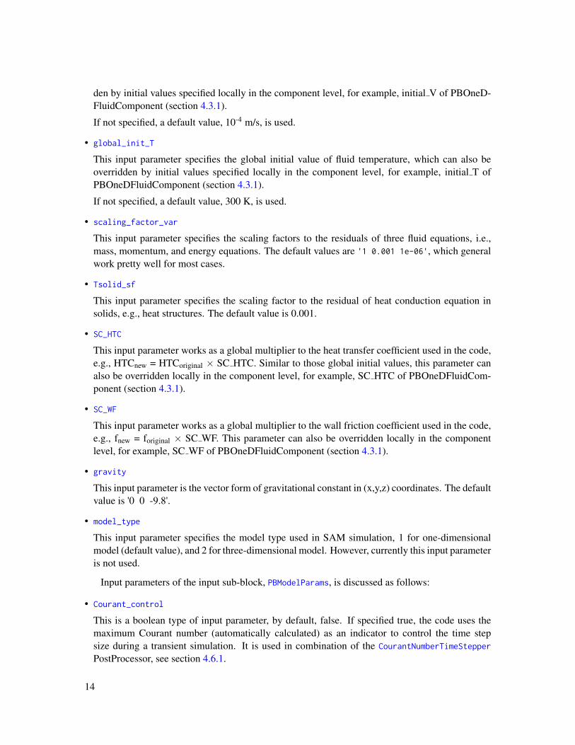
• SC_HTC

This input parameter works as a global multiplier to the heat transfer coefficient used in the code,e.g., HTCnew = HTCoriginal × SC HTC. Similar to those global initial values, this parameter canalso be overridden locally in the component level, for example, SC HTC of PBOneDFluidCom-ponent (section 4.3.1).

• SC_WF

This input parameter works as a global multiplier to the wall friction coefficient used in the code,e.g., fnew = foriginal × SC WF. This parameter can also be overridden locally in the componentlevel, for example, SC WF of PBOneDFluidComponent (section 4.3.1).

• gravity

This input parameter is the vector form of gravitational constant in (x,y,z) coordinates. The defaultvalue is '0 0 -9.8'.

• model_type

This input parameter specifies the model type used in SAM simulation, 1 for one-dimensionalmodel (default value), and 2 for three-dimensional model. However, currently this input parameteris not used.

Input parameters of the input sub-block, PBModelParams, is discussed as follows:

• Courant_control

This is a boolean type of input parameter, by default, false. If specified true, the code uses themaximum Courant number (automatically calculated) as an indicator to control the time stepsize during a transient simulation. It is used in combination of the CourantNumberTimeStepper

PostProcessor, see section 4.6.1.

14

• variable_bounding

This input parameter specifies if variables bounding should be applied to the main fluid variables,i.e., pressure, velocity, and temperature. By default, it is false, i.e., no bounding is applied.

• P_bounds, T_bounds, and V_bounds

These input parameters specify the bounds for the three main fluid variables. The default valuesare: P_bounds = '0 1.0e8' Pa, V_bounds = '-1.0e-3 1.0e3' m/s, and T_bounds = '100 1.2e3'

K. These bounds are only applied when variable_bounding = true.

• fluid_conduction

This input parameter specifies if axial heat conduction effect of the fluid should be modeled,which, if modeled, would be included in the fluid energy equation. Such an effect is generallyonly important in applications where high thermal-conductivity fluids, such as liquid metals, areused. An example application is sodium-cooled fast reactor analysis. For most other applications,it is safe to not include this effect.

• passive_scalar

This input parameter accepts a list of names of passive scalars that are passively transported withfluid flow. For example, passive_scalar = 'particle1 particle2 particle3'.

• global_init_PS

This input parameter specifies the global initial values of passive scalars. For example, global_init_PS= '10.0 80.0 20.0'. Similar to fluid properties, such as pressure, this global initial conditioncould be overridden by locally specified initial conditions in in the component level, for example,initial PS of PBOneDFluidComponent (section 4.3.1).

• passive_scalar_diffusivity

This input parameter specifies the diffusivities of passive scalars in fluid.

• passive_scalar_decay_constant

This input parameter specifies the decay constants of passive scalars. If part of the passive_scalar

list is also defined as decay_heat_precursor, the corresponding decay constants will be used asdecay heat precursor decay constant to compute decay power.

• decay_heat_precursor

This input parameter defines a list of decay heat precursors, each of which must have been speci-fied in the passive_scalar list, to compute decay power.

• p_order

This input parameter specifies the p-order of one- and two-dimensional meshes generated withinthe code. The default value is 1, i.e., first-order.

• pbm_scaling_factors

This input parameter works similarly to the higher level global input parameter, scaling_factor_var.If specified, it overrides scaling_factor_var.

15

• pspg

This input parameter specifies if PSPG stabilization should be used in the fluid mass equation. Bydefault, it is true (1).

• scaling_velocity

This input parameter specifies a reference velocity for scaling to be used in the PSPG scheme.Currently, not used.

• supg

This input parameter specifies if SUPG stabilization should be used in the fluid momentum andenergy equations. By default, it is true (1).

• supg_max

In some extreme cases, for example, fluid velocities very close to 0. The FEM scheme maynot be stable enough to cause unphysical oscillations in numerical solutions. With supg_max =

true, stabilization parameters are adjusted to larger values that help suppress such non-physicaloscillations. In most cases, this is not needed, and it is false (0), by default.

• low_advection_limit

This parameter specifies the lower bound of velocity for advection dominant region. When thevelocity magnitude is smaller than this value, SUPG stabilization scheme is deemed to be unnec-essary, and is turned off. The default value of this input parameter is 10−7 m/s.

An example input of the GlobalParams block is shown below. Note that only a small fractionof the parameters were provides. For other unprovided input parameters, default values are used ifthey are available in the code (as listed in the above input description). If the default value is notavailable, the parameter is not required and its intended function is not activated.

[GlobalParams]global_init_P = 1.2e5global_init_V = 1global_init_T = 628.15scaling_factor_var = '1 1e-3 1e-6'[./ PBModelParams]

p_order = 2[../]

[]

Another example is given on passive scalars. There are eight passive scalars specified in PBModelParams,six of which are also defined as decay_heat_precursor.

[GlobalParams]global_init_P = 1.1e5global_init_V = 0.5global_init_T = 628.15Tsolid_sf = 1e-1

[./ PBModelParams]pbm_scaling_factors = '1 1e-3 1e-6'passive_scalar = 'TEST235 -group0 TEST235 -group1 TEST235 -group2 TEST235 -group3

TEST235 -group4 TEST235 -group5 c1 c6'passive_scalar_diffusivity = '0.0 0.0 0.0 0.0 0.0 0.0 0.0 0.0'passive_scalar_decay_constant = '2.722 1.026 0.314 0.118 0.034 0.012 0.0124

16

3.010 'global_init_PS = '0.0 0.0 0.0 0.0 0.0 0.0 1.94944E+01 3.45288E-13'p_order = 2Courant_control = truedecay_heat_precursor = 'TEST235 -group0 TEST235 -group1 TEST235 -group2 TEST235 -group3

TEST235 -group4 TEST235 -group5 '[../]

[]

4.2 Equation of State (EOS)

SAM provides different options in specifying fluid properties in simulations. Users could choosefrom SAM’s built-in fluid library for commonly-used fluids, including air, nitrogen, helium, sodium,two types of molten salt (Flibe and Flinak), and one simulant oil (DowthermA).

4.2.1 Built-in EOS

SAM provides several built-in EOS for users to pick from. These model requires minimuminput effort, and examples are given as follows:

[./ air_eos]type = AirEquationOfState

[../][./ Helium]

type = HeEquationOfState[../][./N2]

type = N2EquationOfState[../][./ sodium]

type = PBSodiumEquationOfState[../][./ eos]

type = SaltEquationOfStatesalt_type = Flibe

[../][./ eos]

type = SaltEquationOfStatesalt_type = Flinak

[../][./ eos]

type = SaltEquationOfStatesalt_type = DowthermA

[../]

4.2.2 Simple Linearized EOS

SAM also provides another simple equation of state, in which all properties, except density andspecific enthalpy, are constant user-specified input values. The complete input parameters of thissimple equation of state is given as follows:

[./ PTConstantEOS]SC_cp = 1 # Sensitivity coefficient for heat capacitySC_k = 1 # Sensitivity coefficient for thermal conductivitySC_mu = 1 # Sensitivity coefficient for viscositySC_rho = 1 # Sensitivity coefficient for densityT_0 = (required) # Reference temperature

17

beta = 0 # Coefficient of thermal expansioncp = (required) # Specific heatcv = (no_default) # Specific heath_0 = (required) # Reference internal enthalpyk = (required) # Thermal conductivity ,W/(m-K)mu = (required) # Dynamic viscosity , Pa.sp_0 = 100000 # Reference pressurerho_0 = (required) # Reference densitytype = PTConstantEOS

[../]

Density is a linear function of temperature using the provided thermal expansion coefficient, β ,which is calculated as:

ρ = ρ0−ρ0β (T −T0)

Specific enthalpy is also linearly dependent on temperature,

h = h0 + cp(T −T0)

• SC_cp, SC_k, SC_mu, SC_rho

These are sensitivity coefficients that are multiplied to the values of specific heat, thermalconductivity, viscosity, and density of the fluid. They are most useful for uncertainty quantifi-cation, and by default, are zero. For normal applications, they could be simply ignored. Theseparameters are available for all equation of states implemented in SAM code, including thosebuilt-in fluid library discussed earlier.

• p_0

A reference pressure with default value of 105 Pa. For this EOS, it is not used and safe toleave it unspecified.

Other input parameters are self-explanatory and thus not discussed further. An example is givenas follows:

[EOS][./ eos]

type = PTConstantEOSp_0 = 1e5 # Parho_0 = 865.51 # kg/mˆ3beta = 2.7524e-4 # Kˆ{-1}cp = 1272.0 # J/kg-K, at Tavg;h_0 = 7.9898 e5 # J/kgT_0 = 628.15 # Kmu = 2.6216e-4 # Pa-sk = 72 # W/m-K

[../][]

4.2.3 PTFunctionsEOS

In addition to the simple linearized equation of state, SAM also provides PTFunctionsEOS toaccept more complex user-defined fluid properties in terms of pressure and temperature-dependentfunctions. Its input parameters are listed as follows:

18

[./ PTFunctionsEOS]SC_cp = 1 # Sensitivity coefficient for heat capacitySC_k = 1 # Sensitivity coefficient for thermal conductivitySC_mu = 1 # Sensitivity coefficient for viscositySC_rho = 1 # Sensitivity coefficient for densitybeta = (required) # Coefficient of thermal expansioncp = (required) # Specific heatenthalpy = (required) # enthalpyk = (required) # Thermal conductivity , W/(m-K)mu = (required) # Dynamic viscosity , Pa.sp_0 = 100000 # Reference pressurerho = (required) # Densitytype = PTFunctionsEOS

[../]

Among these input parameters, SC_cp, SC_k, SC_mu, SC_rho, and p_0, are the same as described insection 4.2.2. Other parameters are described as follows:

• rho, beta, cp, mu, k, enthalpy (required)

All these input parameters are required. Each of them accepts either a constant value or afunction name, which should have been specified in the [Functions] input block.

An example of using ‘PTFunctionsEOS’ is given as follows:

[Functions][./ enthalpy_fn]

type = PiecewiseLinearx = '428.15 628.15 1028.15 ' # 'x' really means temperature.y = '5.4458 e5 7.9898 e5 1.30778 e6'

[../][]

[EOS][./ eos]

type = PTFunctionsEOSrho = 865.51beta = 0.0cp = 1272.0mu = 2.6216e-4k = 72enthalpy = enthalpy_fn

[../][]

4.2.4 PTFluidPropertiesEOS

To take advantages of many existing built-in fluid properties provided within the MOOSE frame-work, SAM provides an “interface” class, PTFluidPropertiesEOS, to access these fluid propertylibraries. Its input parameter list is given as follows:

[./ PTFunctionsEOS]SC_cp = 1 # Sensitivity coefficient for heat capacitySC_k = 1 # Sensitivity coefficient for thermal conductivitySC_mu = 1 # Sensitivity coefficient for viscositySC_rho = 1 # Sensitivity coefficient for densityfp = (required) # The name of the user object for fluid propertiestype = PTFluidPropertiesEOS

[../]

19

Other than the four sensitivity coefficients, the only user input is a name pointing to a MOOSE-provided fluid property library. This is a required input parameter:

• fp (required)

This is a required parameter that accepts the name of the user object for a MOOSE-providedfluid library. This user object should have been provided in a separate material propertiesinput block, [MaterialProperties].

An example of PTFluidPropertiesEOS usage is given as:

[EOS][./ eos]

type = PTFluidPropertiesEOSfp = fluid_props # Pointing to a user object provided

# in the following MaterialProperties block[../]

[]

[MaterialProperties][./ fluid_props]

type = IdealGasFluidProperties # MOOSE -provided fluid librarygamma = 1.4R = 286.9mu = 2.e-5 #Pa-sk = 0.03

[../][]

4.3 Components

4.3.1 PBOneDFluidComponent

PBOneDFluidComponent is the most basic fluid component in SAM. It represents a unit one-dimensional (1D) component to simulate the 1D fluid flow in a channel. The geometry parameterssuch as the hydraulic diameter, flow area, and length, are provided in the input file. The wall frictionand heat transfer coefficients can be calculated through the closure models based on flow conditionsand geometries or provided by the user input. Internal volumetric heating (or cooling) can be spec-ified by the user input as well. The associated input parameters of the PBOneDFluidComponentComponent block are shown below.

[./ PBOneDFluidComponent]A = (required) # Area of the One -D fluid componentCgb = 1 # Mixing coefficient due to buoyancy

# and geometry effectsCgv = (no_default) # Mixing coefficient due to velocity

# and geometry effectsDh = (required) # Hydraulic diameterHTC_geometry_type = Pipe # Heat transfer geometry typeHTC_user_option = Default # Heat transfer correlation user optionHT_surface_area_density = (no_default) # Heating surface densityHoD = 1 # wire pitch ratio , height to diameterHw = (no_default) # Convective heat transfer coefficientPh = (no_default) # Heated perimeterPoD = 1 # pitch to diameter ratio for parallel bundleSC_HTC = 1 # Sensitivity coefficient for HTC ,

# multiplicativeSC_WF = 1 # Sensitivity coefficient for wall friction ,

20

# multiplicativeWF_geometry_type = Pipe # wall friction geometry typeWF_user_option = Default # user -option for wall friction modelaxial_mixing = 0 # If the 1-D axial mixing model is activatedcomponent_type = PBOneDFluidComponent # The type of the componentend_elems_refinement = 1 # number of element for the end element

# in this OneDCompeos = (required) # The name of EOS to usef = (no_default) # frictionfluid_conduction = (no_default) # if modeling the fluid axial conductionheat_source = 0. # Volumetric heat sourceinitial_P = (no_default) # Initial pressure in the OneDCompinitial_PS = (no_default) # Initial value of passive scalar

# in the OneDCompinitial_T = (no_default) # Initial temperature in the OneDCompinitial_V = (no_default) # Initial velocity in the OneDCompinlet_area_ratio = 1 # Volume area over inlet (jet) areainput_parameters = (no_default) # Name of the ComponentInputParameters

# user objectlam_factor = 1 # a user -input shape factor for laminar

# friction factor for non -circular# flow channels

length = (required) # Length of the OneDCompn_elems = (required) # number of element in this OneDCompn_layers_coolant = (no_default) # Number of layers in the coolant channeloffset = '0 0 0' # Offset of the origin for mesh generationorientation = '0 0 1' # Orientation vector of the componentposition = '0 0 0' # Origin (start) of the componentrotation = 0 # Rotation of the component (in degrees)roughness = 0 # roughness , [m]scalar_source = (no_default) # Volumetric scalar sourcescaling_velocity = (no_default) # a user -input global velocity for PSPG

# schemetao_pspg = (no_default) # tao_pspgtao_supg = (no_default) # tao_supgturb_factor = 1 # a user -input shape factor for turbulent

# friction factor for non -circular# flow channels

type = PBOneDFluidComponent

User_defined_HTC_parameters = '0 0 0 0 0 0 0' # User -defined HTC model parametersUser_defined_WF_parameters = '0 0 0' # User -defined WF model parameterscoolant_density_reactivity_feedback = 0 # Enable coolant density reactivity

# feedback.

coolant_reactivity_coefficients = (no_default) # Coolant reactivity coefficients# (delta_k / k per kg)

coolant_reactivity_coefficients_fn = (no_default) # Coolant reactivity# coefficients function.

[../]

21

Length

Position (x0,y0,z0)

Orientation (dx,dy,dz)

D

(a) A round pipe

Flow Area (A)

Wetted perimeter (P)

(b) A pipe with irregular cross section

Figure 4.1: SAM PBOneDFluidComponent examples.

Each of the input parameters are discussed as follows. Geometry-related input parameters arediscussed first,

• A (required)

Cross-sectional (flow) area of the flow channel. For example, for round pipes, it is simply πD2/4,see figure 4.1.

• length (required)

Length of the flow channel, see figure 4.1.

• position

The origin of the one-dimensional pipe, in (x0, y0, z0), see figure 4.1. The default value is (0, 0,0), i.e., position = '0 0 0'.

• orientation

The orientation vector of the one-dimensional pipe, in (dx, dy, dz), see figure 4.1. Note that itdoes not have to be a unit vector. The default value is (0, 0, 1), i.e., orientation = '0 0 1'.

• n_elemes (required)

Number of elements used for the component in the axial direction.

• Dh (required)

Hydraulic diameter of the flow channel. For round pipes, it is simply the pipe diameter; while forflow channels with irregular shape of cross section, it is calculated as:

Dh =4AP

where A is the cross-sectional area, and P is the wetted perimeter, see figure 4.1.

22

• rotation

Rotation of the component (in degrees), which will be used to construct displaced mesh withinthe code. This is related how SAM internally builds and handles meshes. The default value ofthis input parameter is 0, and in most cases, it is safe to leave it unspecified.

• end_elems_refinement

Number of refined elements for the end elements at the begin and end of this component. Thedefault value is 1, and therefore no refinement. Several examples are shown in figure 4.2 toillustrate how end_elems_refinement works.

(a) n_elemes=5, end_elems_refinement = 1 (default)

(b) n_elemes=5, end_elems_refinement = 2

(c) n_elemes=5, end_elems_refinement = 3

Figure 4.2: PBOneDFluidComponent with end element refinements.

• offset

This parameter accepts an offset, in (dx, dy, dz), from its origin point, i.e., position, such thatthe true origin point of the flow channel becomes (origin + offset). Its default value is (0, 0, 0),meaning no offset at all. This parameter will be depreciated as SAM moves into the real space,instead of the displayed mesh system it is currently using.

Input parameters related to equation of state, and local initial conditions are given as follows:

• eos (required)

The name of equation of state to be used in this component.

• initial_P, initial_V, and initial_T

Local initial condition for pressure, fluid velocity, and temperature, respectively. If specified,these values will override those specified in the global parameter list, and will be used to initializepressure, fluid velocity, and temperature of this component. If not specified, those global initialvalues will be used.

• initial_PS

Local initial conditions for passive scalars. If specified, they override values specified in the globalparameter list. If not specified, the global initial values will be used.

23

The following input parameters are related to how wall frictional coefficients will be calculatedin the fluid component,

• f

A user-specified constant wall frictional coefficient. If not provided, the wall frictional coeffi-cient will be automatically calculated within the code, see section 4.3 of SAM Theory Manual[1]. Whenever provided, this input parameter will shadow all other wall-friction-related inputparameters, such as, WF_user_option, i.e., they will all simply be ignored.

• roughness

Wall roughness. Some wall friction correlations, e.g., the Churchill correlation, require the wallroughness to compute the frictional coefficient. The default value is 0 m.

• WF_geometry_type

Geometry type for SAM to select appropriate wall friction correlations. Currently, there arefour types of geometries for selection: ‘Pipe’ (default), ‘WireWrap’, ‘SquareLattice’, and ‘Plate’,among which, ‘WireWrap’ is typical for sodium fast reactor designs, and ‘SquareLattice’ is typi-cal for light water reactor designs.

• WF_user_option

Users can also directly specify wall friction correlations to be used to compute the frictionalcoefficient, however, it should be noted that some correlations only work with certain geometrytype, WF_geometry_type.

The available options for this parameters are: ‘Default’, ‘BlasiusMcAdams’, ‘ZigrangSylvester’,‘Churchill’, ‘ChengTodreas’, and ‘User’.

First, if the ‘User’ option is selected, SAM will compute the wall frictional coefficient from thefollowing Reynolds number-dependent correlation:

f = A+B×ReC

and SAM is also expecting an additional input parameter, User_defined_WF_parameters, in whichthe user-specified constants are given as ‘A B C’. This user-specified correlation is to be used inboth the laminar and turbulence flow regimes.

For options other than ‘User’, ‘Default’ and ‘BlasiusMcAdams’ are effectively identical: for lam-inar flow, the Darcy’s model will be used, and for turbulent flow, the Blasius correlation is usedfor Reynolds number smaller than 3× 104, and the McAdams correlation for Reynolds numberlarger than 3×104.

The ‘Churchill’ option will use the Churchill model for wall friction coefficient in both the laminarand turbulent flow regimes.

When ‘ZigrangSylvester’ option is selected, the Zigrang-Sylvester correlation will be used for theturbulent flow regime, while for the laminar flow, the Darcy’s model will be used.

When ‘ChengTodreas’ option is selected, the Cheng-Todreas correlation will be used for boththe laminar and turbulent flow regimes. It is also the default option when ‘WireWrap’ type ofgeometry is specified, i.e., WF_geometry_type = WireWrap.

24

D

Pitch (p)A

(a) Square-lattice fuel bundle

A

D

Pitch (p)

(b) Hexagonal-lattice fuel bundle

Figure 4.3: Fuel bundles in (a) square-lattice, typically seen in light water reactor designs; and (b)hexagonal-lattice, typically seen in sodium fast reactor designs.

Users are referred to section 4.3 of the SAM Theory Manual [1] for more details of the wallfriction correlations.

• User_defined_WF_parameters

As discussed in WF_user_option, when WF_user_option = User, this input parameter accepts aset of three values for ‘A B C’ to compute use-provided wall friction factor. If WF_user_option =

User, this input parameter is expected from user input. The default values are '0 0 0'.

• PoD

This parameter defines the pitch (p) to diameter (D) ratio in rod bundles, see figure 4.3. This ratiois to be used to compute wall friction factor in, for example, the Cheng-Todreas correlation, andconvective heat transfer coefficient in, for example, the Kazimi-Carelli correlation.

• HoD

This parameter defines ratio of “wire lead length” (H) to rod diameter (D), see figure 4.4. Cur-rently, this parameter is only used in the Cheng-Todreas correlation to compute wall friction factorin the wire-wrapped fuel bundle geometry.

• lam_factor and turb_factor

A user-input shape factor for laminar/turbulent flow friction factor for non-circular flow channels.Their default values are both 1.0. Basically, they work as multipliers that are multiplied to thevalues computed from wall friction correlations other than user-specified constant wall frictionalcoefficient f and user-specified Reynolds number-dependent correlation WF_user_option.

• SC_WF

This is the same wall friction coefficient multiplier parameter as defined in the global parameterlist, section 4.1. If specified in this component, it will override the globally defined parameterlocally, i.e., in this component.

The following input parameters are related to wall heat transfer,

• Hw

A user-specified constant wall heat transfer coefficient. If not provided, the wall heat transfercoefficient will be automatically calculated within the code, see section 4.2 of SAM Theory Man-ual [1]. Whenever provided, this input parameter will shadow all other wall-heat-transfer-relatedinput parameters, such as, HTC_user_option, i.e., they will all simply be ignored.

25

H

Figure 4.4: Typical SFR wire-wrapped rod configuration.

• Ph

This parameter is the heated perimeter. If heat transfer takes place on the entire wetted perimeter,the heated perimeter is the same as the wetted perimeter, see figure 4.1. For fuel bundles shownin figure 4.3, assuming all fuel rods are heated, the heated perimeters are πD and πD/2 for (a)square-lattice and (b) hexagonal-lattice fuel bundles, respectively. However, it is not always truethat the heated perimeter is the same as the wetted perimeter. If, for example, one of the rod in4.3 (a) is unheated, the heated perimeter is 3πD/4, instead of πD, which is the value of wettedperimeter.

This is an optional input parameter without a default value given. If specified, it will be used tocompute the heat transfer area density, see HT_surface_area_density.

• HT_surface_area_density

This parameter accepts user-specified value for heat transfer surface area density, aw, which isheat transfer surface area per fluid volume [m2/m3]. In most cases, it is computed as the ratio ofheated perimeter to cross-sectional flow area,

aw =Ph

A

For a round pipe, as shown in figure 4.1 (a), it is:

aw =Pheated

A=

πDπD2/4

=4D

For fuel bundles, as for example shown in figure 4.3 (b), it is:

aw =Pheated

A=

3× πD6

A

26

Care should be taken when providing this parameter, as it often depends on how input modelis set up. If not specified correctly, often energy imbalance between fluid components and heatstructures would be introduced.

As for user input, this is an optional input parameter without a default value given. If the heatedperimeter, Ph, is specified, heat transfer area density is computed from its definition, aw = Ph/A.Users can also specify a constant value for aw. If neither heated perimeter nor this parameter isgiven, it is automatically assumed that the heated perimeter is the same as the wetted perimeter,and thus:

aw =Ph

A=

PA=

4Dh

in which P is the wetted perimeter.

• HTC_geometry_type

Geometry type for SAM to select appropriate heat transfer coefficient correlations. There arefour types channel geometries available in SAM, “Pipe (default)”, “Bundle”, “Vertical-Plate”,and “Horizontal-Plate”1.

• HTC_user_option

Similar to wall friction correlation, users can also directly specify correlations to compute heattransfer coefficient. The available options for this parameters are: ‘Default’, ‘NotterSleicher’,‘Aoki’, ‘ChengTak’, ‘Mikityuk’, ‘ModifiedSchad’,‘GraberRieger’, ‘McAdams’, ‘ChurchillChu’,‘GaddisGnielinski’, ‘UserForced’ and ‘UserNatural’.

If this input parameter is not specified, SAM goes to ‘default’ options to select appropriate heattransfer coefficient correlations depending on combination of heat transfer geometry, fluid type(liquid metal or not), and flow condition (laminar or turbulent). For pipe geometry, the defaultcorrelation for liquid metal (Pr < 0.1) is the Seban-Shimazaki correlation (see section 4.2 of SAMTheory Manual [1]); for fluids other than liquid metal, SAM picks the largest value among thosecomputed from the Dittus-Boelter correlation, the Churchill-Chu correlation, and the correlationfor forced laminar flow (Nu = 4.36). For fuel bundle geometry, the default correlation for liquidmetal is the same as used for pipe geometry. For non-liquid metal fluids, SAM picks the largestvalue among those computed from the Inayatov model (modified Dittus-Boelter correlation forfuel bundle geometry), the Churchill-Chu correlation, and the correlation for forced laminar flow(Nu = 4.36).

For pipe geometry, users can also select one of the following correlations, ‘NotterSleicher’, ‘Aoki’or ‘ChengTak’ for liquid metal, or one from ‘McAdams’ and ‘ChurchillChu’ for non-liquid metalfluids. For fuel bundle geometry, available options are ‘Mikityuk’, ‘ModifiedSchad’, and ‘Graber-Rieger’ for liquid metal; and ‘McAdams’, ‘ChurchillChu’, and ‘GaddisGnielinski’ for non-liquidmetal fluids.

SAM also allows users to specify user-defined correlations. Users could select the ‘UserForced’option (for forced convection), and then specify a set of 7 numbers, i.e.,

[Nu0,a,b,c,d,e, f ]

1Vertical-Plate and Horizontal-Plate have not been treated yet.

27

in the User_defined_HTC_parameters input parameter, which will be used to compute the Nusseltnumber in the form of:

Nu = Nu0 +a(

Reb + c)

Prd (1+ eRe f )0.1

Users could also select the ‘UserNatural’ option (for natural convection), and then specify a setof 3 numbers in the User_defined_HTC_parameters input parameter,

[Nu0,a,b]

which will be used to compute the Nusselt number in the form of:

Nu = Nu0 +aRab

For heat transfer coefficients, users are referred to SAM theory manual [1] for more details.

• User_defined_HTC_parameters

This input parameter expects either a set of 7 numbers when HTC_user_option = UserForced, ora set of 3 numbers when HTC_user_option = UserNatural (see the previous item). The defaultvalues are ‘0 0 0 0 0 0 0’.

• SC_HTC

This is the same heat transfer coefficient multiplier parameter as defined in the global parameterlist, section 4.1. If specified in this component, it will override the globally defined parameterlocally, i.e., in this component.

Input parameters related to reactivity feedback model are given as follows:

• coolant_density_reactivity_feedback

If specified true, this input parameter enables coolant density reactivity feedback. By default, it isfalse.

• n_layers_coolant

This parameter specifies the number of layers of coolant in the flow channel. In combina-tion of coolant_reactivity_coefficients or coolant_reactivity_coefficients_fn, the averagecoolant density in each of these layers will be used to compute the total reactivity feedback in thisflow channel. If not specified, it takes the value of number of elements, i.e., n_elems.

• coolant_reactivity_coefficients

This parameter specifies a list of coolant reactivity coefficients. If there is only one value in thislist, this value will be used in all layers of coolant to compute total reactivity feedback. Otherwise,the total number of values in this list should be equal to number of layers, i.e., n_layers_coolant(if specified) or n_elems.

• coolant_reactivity_coefficients_fn

The parameter specifies a function (name) to be used to compute coolant reactivity coefficients.The function should be spatially distributed along the channel’s axial direction. The reactivitycoefficient will be sampled in the middle point of each layer of coolant.

28

All other input parameters are discussed as follows:

• tao_supg

An optional input parameter to accept user-specified SUPG stabilization parameter, τSUPG. If notspecified, τSUPG is automatically computed within the code. It is not recommended to specify thisparameter.

• tao_pspg

An optional input parameter to accept user-specified PSPG stabilization parameter, τPSPG. If notspecified, τPSPG is automatically computed within the code. It is not recommended to specify thisparameter.

• scaling_velocity

An optional input parameter to accept user-specified reference velocity (magnitude) to computePSPG stabilization parameter, τPSPG. If not specified, SAM automatically picks appropriate ve-locity magnitude to compute τPSPG. It is not recommended to specify this parameter.


This input parameter overrides the one specified in the global parameter list, which specifies ifaxial heat conduction effect of the fluid should be included in the fluid energy equation.

• heat_source

This input parameter specifies a direct volumetric heating source to the fluid. A number can besimply specified to assign a constant value as the volumetric heating source. A function name,which must have been given in the [Function] input block, can also be given to this input param-eter, so the volumetric heating source will be calculated from this given function.

• scalar_source

This input parameter specifies a list of volumetric sources to the passive scalar variables. Similarto heat_source, both numbers and function names are acceptable options. In addition, numbersand function names could be mixed in the same list.

• axial_mixing

This input parameter specifies if the one-dimensional axial mixing model should be activated.The default value is false, i.e., axial mixing model is not activated.

• inlet_area_ratio

This input parameter specifies the ratio of volume area to inlet (jet) area for the one-dimensionalaxial mixing model. The default value is 1.0.

• Cgv

This input parameter specifies the mixing coefficient due to velocity and geometry effects for theone-dimensional axial mixing model. The default value is half of the inlet_area_ratio value.

29

• Cgb

This input parameter specifies the mixing coefficient due to buoyancy and geometry effects forthe one-dimensional axial mixing model. The default value is 1.0.

• input_parameters

This input parameter is designed to allow SAM input components share common features. Forexample, in a flow loop consisting of many pipes of the same type, this input parameter allowsthat these common features (e.g., flow area, hydraulic diameter, etc.) are to be inputted for onlyonce. The details are provided in section 4.4.

An example input block is given as follows:

[Components]......[./ pipe1]

type = PBOneDFluidComponenteos = eos # The equation -of-stateposition = '0 0 0' # The origin of this componentorientation = '0 0 1' # The orientation of the componentA = 0.01 # Area of the One -D fluid componentheat_source = 0 # Volumetric heat sourcef = 0.01 # Specified friction coefficientDh = 0.01 # Equivalent hydraulic diameterlength = 1 # Length of the componentn_elems = 100 # Number of elements used in discretization

[../][]

4.3.2 HeatStructure

HeatStructure is the most basic solid structure component in SAM. It represents a unit one-Dor two-D component in Cartesian or cylindrical coordinates to simulate the heat conduction in solidstructures. The geometry parameters such as the thickness and length are provided in the inputfile. Temperature-dependent solid material properties can be provided in tabular or functional formuser-supplied data. Internal volumetric heating can be specified by the user input. Input parametersof HeatStructure is given as follows:

[./ HeatStructure]Ts_init = (no_default) # Initial temperatureaxial_offset = 0 # Axial offset for cylindrical heat structuresdepth_plate = (no_default) # depth of plate in case of plate geometry.

# will be used to calculate the volume.dim_hs = 2 # Dimension of the geometry (1 = 1D, 2 = 2D)elem_number_axial = 1 # Number of axial elements of heat structureelem_number_radial = (required) # Number of radial elements of heat structureend_elems_refinement = 1 # number of element for the end element

# in this Componentheat_source_solid = 0 # heat source in solidhs_names = (no_default) # User given heat structure nameshs_power = (no_default) # total power in the heat structure.hs_power_shape_fn = (no_default) # axial power shape of the heat structure.hs_type = plate # Geometry type of the heat structureinput_parameters = (no_default) # Name of the ComponentInputParameters user objectlength = (required) # Length of the heat structurematerial_hs = (required) # Name of the material used in the heat structureoffset = '0 0 0' # Offset of the origin for mesh generation

30

orientation = '0 0 1' # Orientation vector of the componentposition = '0 0 0' # Origin (start) of the componentpower_fraction = (no_default) # fraction of total power goes into different blocks.radius_i = (no_default) # the radius of the inner wall of the heat

# structure , needed when the hs is a cylinderrotation = 0 # Rotation of the component (in degrees)width_of_hs = (required) # Width of heat structure

[../]

Each of these input parameters are discussed as follows:

• position, orientation, rotation, offset

These input parameters are defined the same way as discussed in section 4.3.1. Also, see figure4.5 for reference.

• dim_hs

It specifies how the heat structure is modeled, either in one-dimensional (dim_hs = 1) or two-dimensional (dim_hs = 2). The default and recommended value is 2, i.e., two-dimensional.

• Ts_init

The initial temperature for the heat structure. If not specified, it seeks the global initial temperature(see global_init_T in section 4.1) as the initial temperature.

• hs_type

Geometry type of the heat structure, which can be either of ‘plate’ (default) or ‘cylinder’ type.Note that this input parameter is case insensitive, e.g., ‘Plate’ is equivalent to ‘plate’. An example2D plate type of heat structure is shown in figure 4.5.

• hs_names

This input parameter specifies a vector of names for each layer of heat structure. If not specified,SAM automatically creates names for each layer of heat structure. For example, in figure 4.5, theautomatically generated names for the two layers would be: <HS name>:hs0 and <HS name>:hs1.

• elem_number_axial

Number of elements in the axial direction (along the length direction, see 4.5) of 2-D heat struc-ture, or number of intervals between 1-D heat structures if it is 1-D heat structure. The defaultvalue is 1. In figure 4.5, elem_number_axial = 4.

• elem_number_radial (required)

This input parameter accepts a vector of numbers that specify the number(s) of elements to beused for each layer of heat structure in the wall-thickness direction. As for example, in figure 4.5,elem_number_radial = '3 4'.

• width_of_hs (required)

This input parameter specifies a vector of thickness for the layer(s) of heat structure. The size ofthis input vector should be the same as n_wall_elems. As for example, in figure 4.5, width_of_hs= 'δ1 δ2'.

31

δ2δ1

depth

length

Position (x0,y0,z0)

Orientation (dx,dy,dz)

Figure 4.5: An example of two-dimensional plate type of heat structure.

• material_hs (required)

This input parameter specifies a vector of heat structure material name(s) for the layer(s) of heatstructure, for example, material_wall = 'SS-304 Wall-Material-2'.

• heat_source_solid

As one of user-specified heat source input options, this input parameter accepts a constant numberthat is used to specify a uniformly distributed constant volumetric heat source (W/m3) in the entireheat structure. The default value is 0. If more complex heat source input than this simple constantvalue is desired, SAM provides other input options, see hs_power.

• hs_power and power_fraction

hs_power specifies the total power, in [W], of the heat structure. If power_fraction is not furtherspecified, it is assumed that the total power is uniformly distributed on the entire heat structure,and therefore, the volumetric heat source is calculated as total power divided by total volume ofthe heat structure.

In case that power is not uniformly distributed, power_fraction accepts a vector of values thatspecifies the fraction of the total power for each layer of heat structure. The size of this vectorhas to be the same as the number of layers in the heat structure. For example, in figure 4.5, onecould specify hs_power = 1000 and power_fraction = '0.9 0.1', and thus 90% of the total powergoes to the first layer (to the left), and 10% goes to the second layer (to the right). Volumetricheat source in each layer of heat structure is then calculated as power in this heat structure layer

32

divided by the solid volume of this heat structure layer.

• hs_power_shape_fn

This input parameter accepts a function name, which can be a function of time and/or space.It is important to note that the function value, which could be both temporal and spatial de-pendent, is multiplied to local volumetric heat source (see previous two items), and there is nore-normalization of total power.

• depth_plate

This input parameter is only required when hs_power is specified and the heat structure type is“plate”. It is required to compute the volume of each heat structure layer. For example, in figure4.5, the volume of the first heat structure layer is calculated as: Length ×δ1× depth.

• radius_i

This input parameter specifies the inner radius of the left-most wall if the heat structure type iscylinder, see figure 4.7 as an example. The default value is 0, if not specified.


Number of refinement for the end elements in the beginning and ending of the component (in theaxial direction). The default value is 1. It is only available when the heat structure dimensionis two. It usage is similar to the same input parameter for PBOneDFluidComponent, see section4.3.1, and it is normally used in pair with PBOneDFluidComponent in PBHeatExchanger (see section4.3.15).

• axial_offset

Axial offset for cylindrical heat structures

• input_parameters (advanced)

This parameter is similar to that of PBOneDFluidComponent, also see section 4.4.

4.3.3 PBPipe

In SAM, PBPipe is directly inherited from PBOneDFluidComponent, with the concept to modela one-dimensional pipe flow and its pipe wall with one layer (or several layers) of HeatStructure,as illustrated in figure 4.6. Its input parameters are therefore a superset of input parameters ofPBOneDFluidComponent and those to define wall heat structures.

The input parameter subset for PBOneDFluidComponent has been discussed in section 4.3.1. Inthis section, only the input parameters to define wall heat structures are discussed:

[./ PBPipe]# Input parameters inherited from PBOneDFluidComponent are not listed.

HS_BC_type = Adiabatic # Heat structure boundary condition typeT_amb = 300 # ambient temperatureT_wall = 600 # Fixed Temperature BC at the outer pipe wall surfaceTwall_init = (no_default) # Initial wall temperaturedim_wall = 2 # The dimension of the mesh used for the wall:

# 1 = 1D, 2 = 2D (default ).disp_mode = 1 # 1.0 for +y display , -1.0 for -y display.

33

PBOneDFluidComponent

HeatStructure

Figure 4.6: SAM’s PBPipe component, which consists of a PBOneDFluidComponent to model theone-dimensional fluid flow and one layer (or several layers) of HeatStructure to model its wall.

# More complicated display modes are necessaryh_amb = (no_default) # convective heat transfer coefficient with ambientheat_source_solid = (no_default) # heat source in solidhs_type = plate # Geometry type of the heat structurematerial_wall = (required) # Name of the material used in the walln_wall_elems = (required) # number of elements in the wallname_comp_right = (no_default) # The name of the right liquid volume

# connected to the heat structureqs_wall = (no_default) # Heat flux at the outer pipe wall surfaceradius_i = (no_default) # the radius of the inner pipe wallwall_thickness = (required) # Thickness of the wallinput_parameters = (no_default) # Name of the ComponentInputParameters

# user object[../]

The detailed descriptions of these heat structure-related input parameters are given as follows:

• Twall_init

The initial wall temperature for heat structures. If not specified, it first seeks local initial fluidtemperature (see initial_T in section 4.3.1) as initial wall temperature; if local initial fluid tem-perature is neither given, it then seeks the global initial temperature (see global_init_T in section4.1) as the initial wall temperature.

• dim_wall

The same as dim_hs in section 4.3.2, it specifies how the wall heat structures are modeled, ei-ther in one-dimensional (dim_wall = 1) or two-dimensional (dim_wall = 2). The default andrecommended value is 2, i.e., two-dimensional.

• hs_type

Geometry type of the heat structure, which can be either of ‘plate’ (default) or ‘cylinder’ type.Note that this input parameter is case insensitive, e.g., ‘Plate’ is equivalent to ‘plate’. This is thesame as hs_type in section 4.3.2.

• radius_i

34

This input parameter specifies the inner radius of the pipe wall, if a cylinder type of heat struc-ture(s) is used to model pipe wall, see figure 4.7. If not specified, it takes half of the hydraulicdiameter value, i.e., Dh/2.

• n_wall_elems (required)

This input parameter accepts a vector of numbers that specify the number(s) of elements to beused for each layer of heat structure in the wall-thickness direction. As for example, in figure 4.7,n_wall_elems = '2 3'. This parameter is the same as elem_number_radial in section 4.3.2.

ri

Figure 4.7: An input example of PBPipe with two layers of heat structures to model its wall. Forexample, it could represent a layer of metal wall and an extra layer of thermal insulation material.

• wall_thickness (required)

This input parameter specifies a vector of wall thickness for the layer(s) of wall heat structure.The size of this input vector should be the same as n_wall_elems. This parameter is the same aswidth_of_hs in section 4.3.2.

• material_wall (required)

This input parameter specifies a vector of heat structure material name(s) for the layer(s) of wallheat structure, for example, material_wall = 'SS-304 Wall-Material-2'. For obvious reason,the size of this input vector should be the same as n_wall_elems. This parameter is the same asmaterial_hs in section 4.3.2.

• heat_source_solid

This input parameter specifies a vector of volumetric heat source (in numbers) of wall heat struc-tures. The vector size has to be the same as n_wall_elems.

• HS_BC_type

This input parameter specifies the boundary condition type for the pipe outer wall surface. Avail-able options for this parameter are: “Adiabatic (default)”, “Temperature”, “Convective”, and“Coupled”.

“Adiabatic”, as its name suggests, sets an adiabatic boundary condition for the pipe outer wallsurface.

35

“Temperature” sets a Dirichlet temperature boundary condition for the pipe outer wall surface.When this boundary condition type is specified, the Dirichlet temperature boundary conditionvalue is also expected from the input file (see T_wall).

“Convective” sets a convective boundary condition to model heat transfer between the pipe outerwall surface and the ambient. Additional input parameters are to be supplied for “Convective”type of boundary condition. This boundary condition type could be supplemented by another twoinput parameters: user-specified ambient temperature (see T_amb) and user-specified heat transfercoefficient (see h_amb). In addition, a user-specified wall heat flux could be directly given on thepipe outer wall surface (see qs_wall).

“Coupled” sets a conjugate heat transfer boundary condition for the pipe outer wall surface. Inthis case, the volume component, with which the outer surface transfers heat, has to be specifiedin the name_comp_right.

• T_wall

Pipe outer wall surface temperature in case that “Temperature” is specified for HS_BC_type. It hasto be a number, and the default value for this input parameter is 600 K.

• T_amb and h_amb

When “Convective” is specified for HS_BC_type, T_amb accepts user-specified ambient temper-ature, and h_amb accepts user-specified heat transfer coefficient. Both input parameters accepteither a number or a function name. The default value for T_amb is 300 K.

• qs_wall

When “Convective” is specified for HS_BC_type, besides T_amb and h_amb, a user-specified wallheat flux could be directly given to the pipe outer wall surface. It can be either a number of afunction name.


See section 4.4.

4.3.4 PBCoreChannel

PBCoreChannel simulates the average coolant flow in rod bundles and heat conduction inside afuel rod, as well as the convective heat transfer between the coolant and the fuel rod. It is com-posed of a PBOneDFluidComponent and a HeatStructure. This is also the so-called “Single-Channel”approach to model the fuel assembly. Axial power profiles and the power fractions of total reactorpower can be specified for the component. If an outer structure (duct wall) is added to PBCoreChan-nel, it becomes PBDuctedCoreChannel, which simulates the ducted fuel assemblies as those in SFRs.

When more complex PBCoreChannel is needed to model the reactor fuel assemblies havingdifferent axial regions, FuelAssembly or DuctedFuelAssembly are provided in SAM.

From thermal-hydraulics point of view, PBCoreChannel is quite similar to PBPipe, both of whichconsist of a 1-D fluid flow model and a heat structure, although PBPipe assumes heat structures tobe pipe walls, while PBCoreChannel assumes heat structures to be fuel rods, figure 4.8. The majordifference between these two components is that PBCoreChannel has a built-in interface to interactwith ReactorPower component. It receives power as heat source from the ReactorPower component,

36

(a)

δ2δ1

(b)

Figure 4.8: PBCoreChannel component (a) SAM’s PBCoreChannel component simulates the aver-age coolant flow in rod bundles and heat conduction inside a fuel rod; and (b) An example meshused in the PBCoreChannel component, 2-D mesh for heat structure and 1-D mesh for fluid flow.

and also provides the capability to model reactivity feedback. The three types of reactivity feedbackmechanisms include fuel’s Doppler effect, fuel expansion effect, and coolant density effect (viaPBOneDFluidComponent).

The full list of input parameters are given in the following table. Most of them are the same asthose for PBOneDFluidComponent (section 4.3.1) or HeatStructure (section 4.3.2).

[./ PBCoreChannel]A = (required) # See PBOneDFluidComponentDh = (required) # See PBOneDFluidComponentHTC_geometry_type = Pipe # See PBOneDFluidComponentHTC_user_option = Default # See PBOneDFluidComponentHoD = 1 # See PBOneDFluidComponentHw = (no_default) # See PBOneDFluidComponentPh = (no_default) # See PBOneDFluidComponentPoD = 1 # See PBOneDFluidComponentSC_HTC = 1 # See PBOneDFluidComponentSC_WF = 1 # See PBOneDFluidComponentend_elems_refinement = 1 # See PBOneDFluidComponenteos = (required) # See PBOneDFluidComponentf = (no_default) # See PBOneDFluidComponentfluid_conduction = (no_default) # See PBOneDFluidComponentinitial_P = (no_default) # See PBOneDFluidComponentinitial_PS = (no_default) # See PBOneDFluidComponentinitial_T = (no_default) # See PBOneDFluidComponentinitial_V = (no_default) # See PBOneDFluidComponentn_elems = (required) # See PBOneDFluidComponentWF_geometry_type = Pipe # See PBOneDFluidComponentWF_user_option = Default # See PBOneDFluidComponentlam_factor = 1 # See PBOneDFluidComponentlength = (required) # See PBOneDFluidComponent

37

orientation = '0 0 1' # See PBOneDFluidComponentposition = '0 0 0' # See PBOneDFluidComponentrotation = 0 # See PBOneDFluidComponentroughness = 0 # See PBOneDFluidComponentscalar_source = (no_default) # See PBOneDFluidComponentscaling_velocity = (no_default) # See PBOneDFluidComponenttao_pspg = (no_default) # See PBOneDFluidComponenttao_supg = (no_default) # See PBOneDFluidComponentturb_factor = 1 # See PBOneDFluidComponentHT_surface_area_density = (no_default) # See PBOneDFluidComponentUser_defined_HTC_parameters = '0 0 0 0 0 0 0' # See PBOneDFluidComponentUser_defined_WF_parameters = '0 0 0' # See PBOneDFluidComponentn_layers_coolant = (no_default) # See PBOneDFluidComponentcoolant_density_reactivity_feedback = 0 # See PBOneDFluidComponentcoolant_reactivity_coefficients = (no_default) # See PBOneDFluidComponentcoolant_reactivity_coefficients_fn = (no_default) # See PBOneDFluidComponent

Ts_init = (required) # See HeatStructuredim_hs = 1 # See HeatStructureheat_source = 0. # See HeatStructurematerial_hs = (required) # See HeatStructurepower_fraction = (no_default) # See HeatStructurepower_shape_function = (no_default) # See HeatStructurewidth_of_hs = (required) # See HeatStructure

assembly_type = RodBundle # Fuel assembly geometry typecoupled_axial_expansion = 0 # If using the displacement from

# external thermo -mechanical module.depth = 1 # The dimension of plate fuel in the

# third direction , melem_number_of_hs = (required) # Number of elements of each heat structurefuel_type = plate # Geometry type of the fuelmesh_disp_gap = 0.005 # Mesh offset when creating heat structure

# meshesn_assemblies = 1 # number of represented assembliesn_heatstruct = (required) # Number of heat structuresname_of_hs = (required) # User given heat structure namesn_rods = (no_default) # number of fuel rods per fuel assembly

eutectic_condition_expansion = 1 # If using the free expansion# model.

fuel_axial_expansion_reactivity_feedback = 0 # Enable fuel axial reactivity# feedback.

fuel_axial_expansion_reactivity_fn = (no_default) # Axial reactivity function name.fuel_doppler_reactivity_coefficients = (no_default) # Fuel Doppler reactivity

# coefficients# (delta_k / k per kg)

fuel_doppler_reactivity_coefficients_fn = (no_default) # Fuel Doppler reactivity# coefficients# (delta_k / k per kg)

fuel_doppler_reactivity_feedback = 0 # Enable fuel Doppler reactivity# feedback.

n_layers_axial_expansion = (no_default) # Number of layers for fuel axial# expansion reactivity feedback.

n_layers_doppler = (no_default) # Number of layers in the fuel# rod for fuel Doppler reactivity# feedback.

input_parameters = (no_default) # Name of the ComponentInputParameters# user object

[../]

• n_assemblies

38

Number of assemblies grouped together that is represented by this PBCoreChannel component.

• elem_number_of_hs (required)

Number of radial elements of heat structure. See elem_number_radial in section 4.3.2.

• Ts_init (required)

The initial temperature for the heat structure, same as Ts_init in section 4.3.2, however this is arequired input parameter for PBCoreChannel component.

• n_heatstruct (required)

Number of heat structures. In some cases that no heat structures should be modeled in this com-ponent, specify zero to this parameter, and at the same time, specify “None” to fuel_type. Whenheat structure is modeled, a company component, ReactorPower is expected in the input file,which provides power to this component and accepts reactivity feedback from this component(optional).

• name_of_hs (required)

This input parameter is similar to hs_names of HeatStructure, however, it is a required inputparameter for this component. It accepts a vector of names, which specify the name of each heatstructure of this component.

• dim_hs

The dimension of the mesh used for the heat structure, same as dim_hs in section 4.3.2. However,the default value here is 1.

• fuel_type

Same as hs_type in section 4.3.2. It can be “None” if no fuel rod is modeled.

• depth

The depth of plate type of fuels, the same as depth_plate in section 4.3.2


It is defined, but not used in this component.

• mesh_disp_gap

This input parameter specifies mesh offset in the y-direction, with respect to the fluid componentmesh, when creating heat structure meshes. The default value for this parameter is 0.005 [m].

• n_rods

Number of fuel rods per fuel assembly. This parameter is only required when assembly type is“Block-Channel”.


It is defined, but not used in this component.

39

• assembly_type

This parameter specifies the assembly type of this PBCoreChannel component. Available optionsinclude “RodBundle” (default), “Plates”, and “Block-Channel”. If “Block-Channel” is specified,an additional input parameter n_rods is expected.

• fuel_axial_expansion_reactivity_feedback

This parameter specifies if reactivity feedback due to fuel axial expansion should be considered.By default, it is False (not considered). When it is specified True, additional input parameters areexpected from user input (see discussion that follows).

• n_layers_axial_expansion

When fuel_axial_expansion_reactivity_feedback = True, this parameter specifies the numberof fuel layers in the axial direction (Nlayer). The length of each of these layers is assumed to bethe same, and thus it is equal to total fuel length divided by Nlayer. If not specified, this parametertakes the number of fluid elements (the same as the number of heat structure elements in the axialdirection) as its default value. Averaged axial displacement in fuel rod will be calculated in eachof these layers for the component to compute the overall reactivity feedback due to fuel axialexpansion.

• fuel_axial_expansion_reactivity_fn

When fuel_axial_expansion_reactivity_feedback = True, this parameter specifies the name ofa function that will be used to compute the overall reactivity feedback due to fuel axial expansion.

• coupled_axial_expansion

When fuel_axial_expansion_reactivity_feedback = True, this parameter specifies that, if True,fuel axial expansion is computed from codes external to SAM; and if False (default), it will becalculated internally using SAM’s built-in models.

• eutectic_condition_expansion

When fuel_axial_expansion_reactivity_feedback = True, this parameter specifies that, if True(default), eutectic conditions are assumed for fuel and clad expansions; and if False, fuel and cladare assumed to expand freely.

• fuel_doppler_reactivity_feedback

This parameter specifies if reactivity feedback due to fuel’s Doppler effect should be considered.By default, it is False (not considered). When it is specified True, additional input parameters areexpected from user input (see discussion that follows).

• fuel_doppler_reactivity_coefficients_fn

When fuel_doppler_reactivity_feedback = True, this parameter accepts the name of a functionthat computes fuel’s Doppler effect coefficients. The function can be spatial-dependent only. Thevalue is evaluated in the middle of each fuel layer, see n_layers_doppler.

• fuel_doppler_reactivity_coefficients

40

Instead of using a function, it is also possible to directly specify a vector Doppler effect reactivitycoefficients for each fuel layer. This vector could contain only single value, such that it willbe used for all fuel layers. Otherwise, the number of values in this vector shall be the same asn_layers_doppler.

• n_layers_doppler

Similar to n_layers_axial_expansion, this input parameter specifies the number of fuel layers inthe axial direction to compute fuel’s Doppler effect, only needed when fuel_doppler_reactivity

_feedback = True.


See section 4.4.

4.3.5 PBDuctedCoreChannel

PBDuctedCoreChannel is intended to model a fuel subassembly, which consists of a fuel bundlemodeled as a PBCoreChannel and its duct wall modeled as an additional heat structure. Sucha ducted fuel subassembly concept is typical in some sodium fast reactor designs. From user-input point of view, PBDuctedCoreChannel inherits all input parameters from the PBCoreChannelcomponent (see 4.3.4), and requires additional input parameters to describe the duct wall, which arelisted as follows:

[./ PBDuctedCoreChannel]# Input parameters same as those in PBCoreChannel are not listed.

name_of_duct = duct # User given duct wall heat structure namesdim_duct = 2 # Dimension of the geometry (1 = 1D, 2 = 2D)Tduct_init = (no_default) # Initial duct wall temperatureduct_thickness = (required) # Thickness of the duct walln_duct_elems = (required) # number of elements in the duct wallmaterial_duct = (required) # Name of the material used in the duct walldisp_mode = 1 # 1.0 for +y display , -1.0 for -y display.

# More complicated display modes are necessaryname_of_bpc = (no_default) # Adjacent BypassChannel names for the CoreChannelHT_surface_area_density_duct = (required) # duct side heating surface density

[../]

• name_of_duct

This parameter specifies the name of the duct wall. If not specified, the default value is “duct”.

• dim_duct

Similar to dim_hs of HeatStructure, it specifies how duct wall heat structure is modeled, eitherin one-dimensional (1) or two-dimensional (2). The default and recommended value is 2, i.e.,two-dimensional.

• Tduct_init

This parameter specifies the initial temperature for the duct wall. If not specified, it takes theglobal initial temperature, global_init_T (see section 4.1), as the initial duct wall temperature.

41

• duct_thickness (required)

The thickness of the duct wall.

• n_duct_elems (required)

Number of elements to model the duct wall in its thickness direction.

• material_duct (required)

This parameter specifies the duct wall material.

• HT_surface_area_density_duct (required)

This parameter specifies the heat transfer surface area density of the duct wall with respect to theCoreChannel.

• disp_mode

To be added.

• name_of_bpc

This parameter specifies the name of BypassChannel adjacent for the CoreChannel.

4.3.6 PBBypassChannel

PBBypassChannel is just a PBOneDFluidComponent component with additional physics mod-els. It is designed to model the bypass flow in the gaps between fuel assemblies. It includes themodeling of conjugate heat transfer with the neighboring fuel assembly duct walls. It can alsomodel the direct coolant heating as a fraction of the total reactor power and using the same ordifferent axial power shapes.

From user-input point of view, it inherits all input parameters from PBOneDFluidComponent,and requires additional input parameters to describe its neighboring PBDuctedCoreChannels anddirect coolant heating.

[./ PBBypassChannel]# Input parameters same as those in PBOneDFluidComponent are not listed.

name_of_cc = (no_default) # Adjacent CoreChannel namespower_fraction = (no_default) # fraction of reactor power goes into

# this bypass channelpower_shape_function = (no_default) # axial power shape of the channelHT_surface_area_density_second = (no_default) # Heating surface density

[../]

• name_of_cc

This input parameter specifies the names of the two adjacent PBDuctedCoreChannels.

• power_fraction

This input parameter specifies the fraction of reactor power directly goes into this bypass channel.When specified, a ReactorPower component is also expected in the input file that provides thecomputation of reactor power.

42

• power_shape_function

This input parameter accepts a function name, which can be a function of time and/or space. It isimportant to note that the function value, which could be both temporal and spatial dependent, ismultiplied to local volumetric heat source, and there is no re-normalization of total power.

• HT_surface_area_density_second

This input parameter is used in parallel wit HT_surface_area_density inherited from PBOneD-FluidComponent. This parameter specifies aw for the second PBDuctedCoreChannels in the list,while HT_surface_area_density specifies aw for the first one.

4.3.7 PBMoltenSaltChannel

PBMoltenSaltChannel is a component intended to model the core behavior of molten-salt re-actor designs. It is a PBOneDFluidComponent component with additional physics models thataccount for heating due to reactor power and decay curve.

From user-input point of view, it inherits all input parameters from PBOneDFluidComponent,and requires additional input parameters for the extra physics models.

[./ PBMoltenSaltChannel]# Input parameters same as those in PBOneDFluidComponent are not listed.

power_fraction = (no_default) # fraction of reactor power goes into# this molten salt channel

power_product_name = (no_default) # scalar power product source namespower_shape_function = (no_default) # axial power shape of the channelbeta = (no_default) # scalar power product fractionsdecay_curve_power_frac = (no_default) # Power fractions for decay heat curvedecay_heat_curve_names = (no_default) # Decay heat curve names

[../]

• power_fraction

This input parameter specifies the fraction of reactor power directly goes into this bypass channel.When specified, a ReactorPower component is also expected in the input file that provides thecomputation of reactor power. If not specified, it is assumed there is no direct heating to thisPBMoltenSaltChannel.

• power_shape_function

This input parameter accepts a function name, which can be a function of time and/or space. Itis only needed when power_fraction is specified. It is important to note that the function value,which could be both temporal and spatial dependent, is multiplied to local volumetric heat source,and there is no re-normalization of total power. If not specified, SAM takes a default power shapefunction, which is defined as,

f =π

2sin(

πxL

)where x is the axial location, and L is the channel length.

43

• power_product_name

This input parameter specifies a list of passive scalars that this PBMoltenSaltChannel componentwill model as its fission products. These passive scalars should have been defined in the globalparameter, passive_scalar (see section 4.1). The product faction of each scalar is specified inbeta. In addition this user-specified list of passive scalars, PBMoltenSaltChannel also has built-indecay curves for several isotopes, see decay_heat_curve_names.

• beta

This parameter specifies the scalar power product fractions.

• decay_heat_curve_names

This component also provides user input to choose built-in decay curves for several isotopes,including “U235T”, “PU239T”, “U238F”, “PU241T”, and “TEST235”.

4.3.8 FuelAssembly

FuelAssembly or DuctedFuelAssembly (see section 4.3.9) model the reactor fuel assemblies com-posed of multiple PBCoreChannels or PBDuctedCoreChannels, representing different axial regions ofa fuel assembly including the active core, gas plenum, lower and upper reflector, lower and uppershield, etc. The junction components (PBSingleJunction) are also auto-created in FuelAssembly orDuctedFuelAssembly to model the connection among the fluid parts of PBCoreChannel or PBDucted-CoreChannel.

The complete list of input parameters of FuelAssembly is give as,

[./ FuelAssembly]A = (required) # Areas of the OneDCompDh = (required) # Hydraulic diameterHTC_geometry_type = Pipe # Heat transfer geometry typeHTC_user_option = Default # User option heat transfer correlationsHT_surface_area_density = (required) # Heating surface densityHw = (no_default) # Convective heat transfer coefficientPoD = (no_default) # pitch to diameter ratio for parallel bundle

# heat transferSC_HTC = (no_default) # Sensitivity coefficient for HTC , multiplicativeTs_init = (required) # Initial solid temperaturedim_hs = 2 # See PBCoreChannelelem_number_of_hs = (required) # Number of elements of each heat structureeos = (required) # See PBCoreChannelf = (no_default) # frictionhs_type = (no_default) # Geometry type of the fuelinitial_P = (no_default) # Initial pressure in the OneDCompinitial_T = (no_default) # Initial temperature in the OneDCompinitial_V = (no_default) # Initial velocity in the OneDCompjunction_nodalTbc = 1 # if use nodalTbc for junctionslam_factor = (no_default) # a user -input shape factor for laminar friction

# factor for non -circular flow channelslength = (required) # Length of the OneDCompmaterial_hs = (required) # Name of the materials used in the heat

# structuresn_assemblies = 1 # See PBCoreChanneln_elems = (required) # number of element in this OneDCompn_heatstruct = (required) # Number of heat structuresn_zones = (required) # number of zonesname_of_hs = (required) # User given heat structure namesorientation = '0 0 1' # See PBCoreChannel

44

plate_depth = (no_default) # The dimension of plate fuel in the third# direction , m

position = '0 0 0' # See PBCoreChannelpower_fraction = (no_default) # fraction of reactor power goes into this core

# channelpower_shape_function = (no_default) # See PBCoreChannelrotation = 0 # See PBCoreChannelroughness = (no_default) # roughness , [m]scaling_velocity = (no_default) # a user -input global velocity for PSPG schemetao_pspg = (no_default) # tao_pspgtao_supg = (no_default) # tao_supgturb_factor = (no_default) # a user -input shape factor for turbulent friction

# factor for non -circular flow channelswidth_of_hs = (required) # Width of each heat structure

[../]

The input parameters of a FuelAssembly are quite similar to those of a PBCoreChannel. How-ever, as a FuelAssembly consists of multiple PBCoreChannels to represent different axial regionsof a fuel assembly, most of its input parameters require a list of numbers (or strings), instead of asingle number (or string) as in PBCoreChannel. Most of these input parameters could be found inPBCoreChannel or PBOneDFluidComponent and HeatStructure.

• n_zones (required)

This input parameter specifies number or zones, i.e., number of PBCoreChannels, to be used inthe FuelAssembly component along the axial direction.

• A (required)

A list of n zones areas for the n zones PBCoreChannels.

• Dh (required)

A list of n zones hydraulic diameters, Dh, for the n zones PBCoreChannels.

• n_elems (required)

A list of n zones numbers of elements for the one-dimensional flow channel in the axial directionfor the n zones PBCoreChannels.

• HTC_geometry_type

A list of n zones heat transfer geometry types for the n zones PBCoreChannels. For heat transfergeometry types, see section 4.3.1.

• HTC_user_option

A list of n zones heat transfer user options for the n zones PBCoreChannels. For heat transferuser options, see section 4.3.1.

• HT_surface_area_density (required)

A list of n zones heat transfer surface densities, aw, for the n zones PBCoreChannels.

• Hw

A list of n zones wall heat transfer coefficients for the n zones PBCoreChannels.

45

• PoD

A list of n zones pitch-to-diameter ratios for the n zones PBCoreChannels.

• SC_HTC

A list of n zones sensitivity coefficients for heat transfer coefficient for the n zones PBCoreChan-nels.

• Ts_init (required)

A list of n zones heat structure initial temperatures for the n zones PBCoreChannels.

• dim_hs

The dimension of the mesh used for the heat structure of all PBCoreChannels. It does not requirea list of dimensions.

• f

A list of n zones user-specified wall frictional coefficient for the n zones PBCoreChannels.

• hs_type

A list of n zones heat structure types for the n zones PBCoreChannels.

• initial_P, initial_T, and initial_V

A list of n zones initial pressure (temperature, velocity) for the n zones PBCoreChannels.

• junction_nodalTbc

As within the FuelAssembly component, n zones - 1 PBSingleJunctions are automatically createdto connect the n zones PBCoreChannels, this input parameter specifies if ‘nodal Tbc’ is to be usedfor these automatically generated PBSingleJunctions. For ‘nodal Tbc’ of PBSingleJunction, seesection 4.3.22.


A list of n zones user-input shape factors for laminar (turbulent) flow friction factor for non-circular flow channels for the n zones PBCoreChannels.

• length (required)

A list of n zones lengths for the n zones PBCoreChannels.

• n_heatstruct (required)

A list of n zones number of heat structures for the n zones PBCoreChannels. Sum all thesenumbers up, the total number of heat structures, nhs,total , is obtained. For example, in a two-zoneFuelAssembly, if n_heatstruct = '2 3', there are in total 5 heat structures (nhs,total = 5) that willrequire use-inputs for their names, widths, materials, number of elements in its width direction,power fractions, etc. See following discussions.

• elem_number_of_hs (required)

A list of nhs,total numbers of elements for the nhs,total heat structures in the FuelAssembly compo-nent.

46

• material_hs (required)

A list of nhs,total names of materials for the nhs,total heat structures in the FuelAssembly compo-nent.

• power_fraction (required)

A list of nhs,total power fractions that goes to the nhs,total heat structures in the FuelAssemblycomponent.

• plate_depth

A list of n zones values of the dimension of plate fuel in the third direction for the n zonesPBCoreChannels. Only needed for plate type of fuels. Also, see section 4.3.4.

• roughness

A list of n zones wall roughnesses for the n zones PBCoreChannels.

• scaling_velocity, tao_pspg, and tao_supg

A list of n zones scaling velocities (τPSPG, τSUPG) for the n zones PBCoreChannels. Also, seesection 4.3.4.

4.3.9 DuctedFuelAssembly

DuctedFuelAssembly is simply a FuelAssembly (see section 4.3.8) with an outer duct. It inheritsall input parameters from FuelAssembly component, and requires additional input parameters todescribe its outer duct:

[./ DuctedFuelAssembly]# Input parameters same as those in FuelAssembly are not listed.

dim_duct = 2 # Dimension of the geometry (1 = 1D, 2 = 2D)Tduct_init = (no_default) # Initial duct wall temperatureduct_thickness = (required) # Thickness of the duct wallelem_number_of_duct = (required) # number of elements in the duct wallmaterial_duct = (required) # Name of the material used in the duct wallHT_surface_area_density_duct = (required) # duct side heating surface density


[../]

• dim_duct

Similar to dim_hs of HeatStructure, it specifies how duct wall heat structure is modeled, eitherin one-dimensional (1) or two-dimensional (2). The default and recommended value is 2, i.e.,two-dimensional.

• Tduct_init

A list of n zones initial temperatures for the duct wall of the n zones PBDuctedCoreChannels. Ifnot specified, it takes the global initial temperature, global_init_T (see section 4.1), as the initialduct wall temperature.

47

• duct_thickness (required)

A list of n zones duct wall thickness of the n zones PBDuctedCoreChannels.

• elem_number_of_duct (required)

A list of n zones numbers of elements, each of which is to be used to specify the number ofelements in the duct wall for each PBDuctedCoreChannel.

• material_duct (required)

This parameter specifies the duct wall material for all duct walls.

• HT_surface_area_density_duct (required)

A list of n zones heat transfer surface area densities of the duct walls with respect to the PBDuct-edCoreChannels.


See section 4.4.

4.3.10 MultiChannelRodBundle

To improve the heat transfer between the duct wall and coolant flow, a multi-channel rod bundlemodel is developed in SAM to account for the temperature differences between the center regionand the edge region of the coolant channel in a fuel assembly. Similar approach has been proposedin ENERGY (Yang and Joo, 1999), SAS4A/SASSYS-1 (Fanning 2012), as well as the multi-regionporous medium model reported by Yu et al. (2015). The whole fuel assembly can be divided intoa number of regions, as shown in figure 4.9. It is quite remarkable that the volumetric heat fluxin region 1 is significantly less than that in other regions, based on analytical calculations. Eachinner region is modeled as an average core-channel (i.e., a 1-D coolant channel and an average fuelpin). The edge region can be modeled as one core-channel or six core-channels to account for thedifferences in heat transfer with each side of the duct wall. This zoning strategy is also inspiredfrom the authors’ previous experiences in the CFD simulations of the triangle-lattice pin bundles.As shown in the Hu and Yu (2016), large temperature gradient were observed in the coolant regionnear the duct wall, but the temperature distribution elsewhere is very uniform except the hot spotsdue to the wire-wrap effects.

48

flat-to-flat distance

fuel pin diameter

Pitch

Figure 4.9: Sketch of the regions in the multi-channel model.

In the SAM multi-channel model, the fluid regions are modeled as separate parallel channelswith the same pressure drop. For simplicity, it is assumed that there are no mass and momentumexchange between channels. However, the energy exchange is allowed at all axial nodes.

MultiChannelRodBundle assumes that the heat structures are the same for all its automaticallygenerated PBCoreChannels, and thus the same input parameters for heat structure are used for allPBCoreChannels. Also, note that MultiChannelRodBundle does not model the outer duct wall.

Input parameters of MultiChannelRodBundle are given as follows:

[./ MultiChannelRodBundle]Ts_init = (required) # See PBCoreChannels , same for all channelsassem_Dft = (required) # The flat -to-flat distance of the assemblybeta = 0 # turbulent mixing parameterdim_hs = 1 # The dimension of the mesh used for the

# heat structure: 1 = 1D(default), 2 = 2D .elem_number_of_hs = (required) # See PBCoreChannels , same for all channelseos = (required) # See PBOneDFluidComponentinitial_P = (no_default) # Initial pressure in the OneDCompinitial_T = (no_default) # Initial temperature in the OneDCompinitial_V = (no_default) # Initial velocity in the OneDComplam_factor = (no_default) # a user -input shape factor for laminar

# friction factor for non -circular flow channelslength = (required) # See PBCoreChannel , same for all channelsmaterial_hs = (required) # See PBCoreChannel , same for all channelsn_channel = (no_default) # Number of CoreChannelsn_elems = (required) # number of axial elementn_heatstruct = (required) # See PBCoreChannels , same for all channelsn_side = (required) # Number of fuel pin rings

49

n_zones = (required) # Number of zonesname_of_hs = (required) # See PBCoreChannels , same for all channelsorientation = '0 0 1' # See PBOneDFluidComponentpin_diameter = (required) # The fuel pin diameterpin_pitch = (required) # The distance between fuel pin centersposition = '0 0 0' # See PBOneDFluidComponentpower_fraction = (no_default) # See PBCoreChannel , same for all channelspower_shape_function = (no_default) # See PBCoreChannel , same for all channelsradial_power_peaking = (no_default) # radial power peaking factorsrotation = 0 # See PBOneDFluidComponentroughness = (no_default) # roughness , [m]scaling_velocity = (no_default) # a user -input global velocity for PSPG schemetao_pspg = (no_default) # tao_pspgtao_supg = (no_default) # tao_supgturb_factor = (no_default) # a user -input shape factor for turbulent

# friction factor for non -circular flow channelswidth_of_hs = (required) # See PBCoreChannels , same for all channelswire_diameter = 0 # The wire wrap diameter


[../]

• n_zones (required)

Number of zones (regions) of the MultiChannelRodBundle. For example, n_zones = 5 in figure4.9. Note that it is different than the same parameter defined in FuelAssembly (see section 4.3.8),which splits the fuel assembly in the axial direction.

• n_side (required)

Number of fuel pin rings of the MultiChannelRodBundle. As shown in figure 4.9, it is also thesame as the number of fuel pins on the side of MultiChannelRodBundle. In figure 4.9, n_side =

5.

• n_channel (required)

Number of core-channels to be modeled in this MultiChannelRodBundle component. It has to beeither the same as n_zones, such that one core-channel for each zone, or equal to n_zones+5, suchthat the out most zone is modeled as six (6) core-channels and one core-channel for each innerzone. For example, as shown in figure 4.9, if n_channel = 5, one core-channel will be created foreach zone (region) 1 to 5; however, if n_channel = 10, one core-channel will be created for eachzone (region) 2 to 5, while 6 core-channels are to be created for zone (region) 1. One can easilyfigure out that MultiChannelRodBundle currently only supports a hexagonal fuel bundles such asthe one shown in figure 4.9.

• assem_Dft (required)

This parameter specifies the flat-to-flat distance of the assembly, see figure 4.9.

• beta

Turbulent mixing parameter which will be used to compute the turbulent mixing between neigh-boring core-channels. Currently, it accepts a simple number for all mixing parameters. This willbe improved in future implementations.

50

• dim_hs

Same for all core-channels of this MultiChannelRodBundle, it specifies how the heat structure ismodeled, either in one-dimensional (dim_hs = 1) or two-dimensional (dim_hs = 2). The defaultand recommended value is 1, i.e., one-dimensional.

• initial_P, initial_T, and initial_V

A list of n zones initial pressure (,temperature, and velocity) for the n zones PBCoreChannels.


A list of n zones user-input shape factors for laminar (turbulent) flow friction factor for non-circular flow channels for the n zones PBCoreChannels.

• roughness

A list of n zones wall roughnesses for the n zones PBCoreChannels.

• scaling_velocity, tao_pspg, and tao_supg

A list of n zones scaling velocities (,τPSPG, and τSUPG) for the n zones PBCoreChannels. Also,see section 4.3.4.

• wire_diameter

The wire wrap diameter, same for all PBCoreChannels. The default value is zero.

• pin_diameter (required)

The fuel pin diameter, same for all PBCoreChannels, see figure 4.9.

• pin_pitch (required)

The distance between fuel pin centers, see figure 4.9.


See section 4.4.

4.3.11 HexLatticeCore

HexLatticeCore models a reactor core with a hexagonal lattice such as SFRs, as schematicallyshown in figure 4.10. It can automatically generate the core lattice of MultiChannelRodBundleor PBCoreChannel components, and the inter-assembly structures (including duct walls and inter-assembly gaps), based on the geometry information specified in the input.

51

Figure 4.10: Sketch of HexLatticeCore component.

Its input parameters are given as follows:

[./ HexLatticeCore]assem_Dft = (required) # The flat -to-flat distance of the assemblyassem_layout = (required) # The layout of the assembly latticeassem_pitch = (required) # The distance between assembly centersb_multichannel = 0 # if use MultiChannelRodBundle for each assemblyb_radial_heat_transfer = 1 # if modeling radial heat transfer between

# assembliesn_side = (required) # Number of side CoreChannelsorientation = '0 0 1' # See PBOneDFluidComponentposition = '0 0 0' # See PBOneDFluidComponentradial_power_peaking = (no_default) # radial power peaking factorsref_duct = (no_default) # reference heat structure for one side of an

# assembly duct wallref_hs = (no_default) # reference heat structure for intra -assembly gap

# and two duct wallsrotation = 0 # See PBOneDFluidComponent

[../]

• n_side (required)

Number of assemblies on each side of the core. For example, n_side = 2 in figure 4.10, and thetotal number of assemblies in the entire core is 7.

• assem_Dft (required)

The flat-to-flat distance of the assembly, assumed to be the same for all assemblies in the HexLat-ticeCore.

• assem_pitch (required)

The distance between assembly centers, assumed to be the same for all assemblies in the HexLat-ticeCore.

52

• b_multichannel

This input parameter specifies if MultiChannelRodBundle (true) or simply PBCoreChannel (false)should be used to represent each assembly in the core. By default, it is ‘false’, i.e., to use PB-CoreChannel.

• assem_layout (required)

This input parameter accepts a list of names for ComponentInputParameters, which are to beused to automatically create all assemblies within the HexLatticeCore component. The numberof ComponentInputParameters has to be the same as the number of assemblies in the core, and theassemblies are numbered in an order from left to right, and then top to bottom. If b_multichannel= true, it is expected that the list of ComponentInputParameters are of MultiChannelRodBundle-Parameters type, otherwise, PBCoreChannelParameters.

• b_radial_heat_transfer

This input parameter specifies if radial heat transfer between assemblies should be modeled. Iftrue (default), HexLatticeCore component automatically adds duct wall heat structures betweenassemblies, and to the out most boundaries of all assemblies, and models the heat transfer betweenduct walls/gaps and their neighboring core channels.

• ref_hs

If radial heat transfer between assemblies should be modeled, this input parameter accepts aHeatStructureParameters to build duct wall heat structures between two neighboring assemblies.It is recommended that this reference heat structure models three layers of heat structures, includ-ing two duct walls and a layer of gap (modeled as a layer heat structure) between them. It assumesthat all such intra-assemblies heat structures have similar geometries.

• ref_duct

If radial heat transfer between assemblies should be modeled, this input parameter accepts aHeatStructureParameters to build duct wall heat structures for the out most boundaries of allassemblies. This reference heat structure should contain only one layer of duct wall. It assumesthat all duct wall heat structures have similar geometries.

• radial_power_peaking

This input parameter accepts a list of radial power peaking factors for assemblies within theHexLatticeCore component. The number of power peaking factors has to be the same as thetotal number of assemblies. The power fraction that goes to each assembly is simply calculatedas power peaking factor divided by total number of assemblies. If not specified, it assumes thatpower is uniformly distributed across all assemblies.

4.3.12 PBCoupledHeatStructure

PBCoupledHeatStructure simulates a HeatStructure with controlled boundary conditions at thetwo surfaces, such as adiabatic, fixed temperature, convective heat transfer with ambient, or coupledwith 0-D liquid volume or 1-D liquid components. Normally users will not directly use HeatStruc-tures to create their models, but use PBCoupledHeatStructure instead.

53

Most its input parameters are inherited from the base HeatStructure component, see section4.3.2, and additional input parameters are required to setup its left(right) boundary conditions. Thecomplete input parameters of PBCoupledHeatStructure are listed below:

[./ PBCoupledHeatStructure]Ts_init = (no_default) # See HeatStructureaxial_offset = 0 # See HeatStructuredepth_plate = (no_default) # See HeatStructuredim_hs = 2 # See HeatStructureelem_number_axial = 1 # See HeatStructureelem_number_radial = (required) # See HeatStructureend_elems_refinement = 1 # See HeatStructurehs_names = (no_default) # See HeatStructurehs_power = (no_default) # See HeatStructurehs_power_shape_fn = (no_default) # See HeatStructurehs_type = plate # See HeatStructureheat_source_solid = 0 # See HeatStructureinput_parameters = (no_default) # See HeatStructurelength = (required) # See HeatStructurematerial_hs = (required) # See HeatStructureoffset = '0 0 0' # See HeatStructureorientation = '0 0 1' # See HeatStructureposition = '0 0 0' # See HeatStructurepower_fraction = (no_default) # See HeatStructureradius_i = (no_default) # See HeatStructurerotation = 0 # See HeatStructurewidth_of_hs = (required) # See HeatStructure

D_heated_left = (no_default) # Characteristic heated length at left surfaceD_heated_right = (no_default) # Characteristic heated length at right surfaceHS_BC_type = (required) # Heat structure boundary condition typeHw_left = (no_default) # Convective heat transfer coefficient at

# left surfaceHw_right = (no_default) # Convective heat transfer coefficient at

# right surfaceT_amb_left = 300 # left ambient temperatureT_amb_right = 300 # right ambient temperatureT_bc_left = 600 # Fixed Temperature BC at left surfaceT_bc_right = 600 # Fixed Temperature BCT_external_left = (no_default) # Coupled variable for left external temperatureT_external_right = (no_default) # Coupled variable for right external temperatureeos_left = (no_default) # The name of EOS to useeos_right = (no_default) # The name of EOS to useh_external_left = (no_default) # Coupled variable for left external heat

# transfer coefficientsh_external_right = (no_default) # Coupled variable for right external heat

# transfer coefficientsname_comp_left = (no_default) # The name of the left liquid volume connected

# to the heat structurename_comp_right = (no_default) # The name of the right liquid volume connected

# to the heat structureqs_external_left = (no_default) # Coupled variable for left heat fluxqs_external_right = (no_default) # Coupled variable for right heat fluxqs_left = (no_default) # Heat flux at the left surfaceqs_right = (no_default) # Heat flux at the right surface

HTC_geometry_type_left = Pipe # Heat transfer geometry type at left surfaceHTC_geometry_type_right = Pipe # Heat transfer geometry type at left surfaceheat_transfer_area_left = 1 # Convective heat transfer area at left surfaceheat_transfer_area_right = 1 # Convective heat transfer area at right surfaceHT_surface_area_density_left = 1 # Heat transfer surface area density at left surfaceHT_surface_area_density_right = 1 # Heat transfer surface area density at right surface

[../]

54

• HS_BC_type (required)

This input parameter specifies the two boundary condition types for the left and right side ofPBCoupledHeatStructure component. Input options include “Temperature”, “Convective”, and“Coupled”.

If “Temperature” is specified, a Dirichlet type of boundary conditions is used, and it expects anadditional user-input for the boundary condition temperature, see T_bc_left(right).

If “Convective” is specified, a wall heat flux will be used. The wall heat flux could be directlyspecified, see qs_left(right). It is also possible to compute the wall surface flux by providingambient temperature (see T_amb_left(right)) and heat transfer coefficient to the ambient (seeHw_left(right)).

In code coupling computation situations, wall heat flux boundary conditions could be calcu-lated from an external code. Corresponding to the two conditions discussed above, one couldspecify an externally calculated wall heat flux, see qs_external_left(right); or a combina-tion of external temperature and wall heat transfer coefficient, see T_external_left(right) andh_external_left(right).

If “Coupled” is specified, still a wall heat flux will be used, but the fluid temperature comesfrom a neighboring component, either a PBVolumeBranch or a PBOneDFluidComponent, seename_comp_left(right). Heat transfer coefficient to the coupled component can be specified inHw_left(right), and if not specified, they will be automatically computed.

• T_bc_left and T_bc_right

If the left/right boundary condition type is “Temperature”, it accepts the value (or a function) forthe left/right boundary condition temperatures. The default values are 600 K.

• qs_left and qs_right

If the left/right boundary condition type is “Convective”, it accepts the value (or a function) forthe left/right wall heat flux as boundary conditions.

• T_amb_left and T_amb_right; Hw_left and Hw_right

If the left/right boundary condition type is “Convective”, T_amb_left(right)) specifies the ambi-ent temperature, and Hw_left(right)) specifies the wall heat transfer coefficient to compute thewall heat flux. Both of these inputs could be either values or function names. The default valuefor T_amb_left(right) is 300 K.

• qs_external_left and qs_external_right

If the left/right boundary condition type is “Convective”, it accepts the variable name for exter-nally computed left/right wall heat flux as boundary conditions.

• T_external_left and T_external_right; h_external_left and h_external_right

If the left/right boundary condition type is “Convective”, T_external_left(right) specifies anexternally computed ambient temperature, and h_external_left(right) specifies an externallycomputed wall heat transfer coefficient to compute the wall heat flux. Both of these inputs haveto be specified as coupled “variables”.

55

• name_comp_left and name_comp_right

If the left/right boundary condition type is “Coupled”, it accepts the name of the componentcoupled to the left(right) surface of this PBCoupledHeatStructure component. The coupled com-ponent has to be either a PBVolumeBranch or a PBOneDFluidComponent.

• eos_left and eos_right

Only when the left/right boundary condition type is “Coupled”, and the coupled component isof PBVolumeBranch type, it is required to specify the name of equation of state to the left(right)coupled PBVolumeBranch component.

• D_heated_left and D_heated_right

Only when the left/right boundary condition type is “Coupled”, and the coupled component is ofPBOneDFluidComponent type, it specifies the characteristic length to compute wall heat transfercoefficient in the coupled left(right) PBOneDFluidComponent component. If not specified, thecoupled PBOneDFluidComponent uses its hydraulic diameter as the characteristic length for heattransfer.

• HTC_geometry_type_left and HTC_geometry_type_right

Heat transfer geometry type at the left(right) surface. Acceptable options are “Pipe (default)”,“Bundle”, “Vertical-Plate”, and “Horizontal-Plate”.

• HT_surface_area_density_left and HT_surface_area_density_right

Only when the left/right boundary condition type is “Coupled”, and the coupled component is ofPBOneDFluidComponent type, it specifies the heat transfer surface area density of this PBCou-pledHeatStructure component with respect to the coupled left(right) PBOneDFluidComponentcomponent.

• heat_transfer_area_left and heat_transfer_area_right

Only when the left/right boundary condition type is “Coupled”, and the coupled component is ofPBVolumeBranch type, it specifies the left(right) side heat transfer surface area of this PBCou-pledHeatStructure component.

4.3.13 HeatStructureWithExternalFlow

HeatStructureWithExternalFlow is also a HeatStructure-based component similar to PBCou-pledHeatStructure, however with the main purpose to facilitate code-to-code coupling via its bound-ary surfaces, either using MOOSE’s MultiApp infrastructure or using data exchange with non-MOOSE-based application. When using MOOSE’s MultiApp infrastructure, this external MOOSEsimulation (a.k.a., MOOSE subApp) will need a different component, HeatTransferWithExternal-HeatStructure (see section 4.3.14) to realize data exchange. It is always assumed that its left-sidesurface is coupled to an external code, while its right-side surface is reserved for SAM to handle itsboundary condition.

[./ HeatStructureWithExternalFlow]Ts_init = (no_default) # See HeatStructure , NOT USED.axial_offset = 0 # See HeatStructuredepth_plate = (no_default) # See HeatStructure

56

dim_hs = 2 # See HeatStructureelem_number_axial = 1 # See HeatStructureelem_number_radial = (required) # See HeatStructureend_elems_refinement = 1 # See HeatStructurehs_names = (no_default) # See HeatStructurehs_power = (no_default) # See HeatStructurehs_power_shape_fn = (no_default) # See HeatStructurehs_type = plate # See HeatStructurelength = (required) # See HeatStructurematerial_hs = (required) # See HeatStructureoffset = '0 0 0' # See HeatStructureorientation = '0 0 1' # See HeatStructureposition = '0 0 0' # See HeatStructurepower_fraction = (no_default) # See HeatStructureradius_i = (no_default) # See HeatStructurerotation = 0 # See HeatStructurewidth_of_hs = (required) # See HeatStructureheat_source_solid = 0 # See HeatStructure

HS_BC_type = (required) # Heat structure boundary condition typeHw_internal = None # convective heat transfer coefficient

# at SAM Side surfaceT_bc_internal = 600 # Fixed Temperature BCT_external_init = 600 # Initial heat structure temperatureT_identifier_in_file = (no_default) # External temperature identifier

# used in external data fileT_internal = 300 # Sam Side ambient temperaturedelete_data_file = (no_default) # Delete data file after readingeos_internal = None # The name of EOS to useh_external_init = 3000 # Initial heat transfer coefficienth_identifier_in_file = (no_default) # External heat transfer coefficient

# identifier used in external data fileinput_data_file = (no_default) # The file name used to save external

# coupling informationname_comp_internal = None # The name of the Sam Side liquid

# volume connected to the heat structureoutput_data_file = (no_default) # The file name used to save SAM

# output information for couplingoutput_mesh = (no_default) # The mesh used to output SAM dataoutput_template_file = (no_default) # The template file name used to

# save SAM output information for couplingqs_external_init = 0 # Initial heat fluxqs_internal = None # Heat flux at the SAM Side surface

HT_surface_area_density_internal = 1 # heat transfer surface area density# at Sam Side surface

heat_transfer_area_internal = 1 # convective heat transfer area# at Sam Side surface

[../]

• HS_BC_type (required)

This input parameter specifies: 1) a list of two heat structure boundary condition types for theleft-side (coupled to an external code) and right-side (within SAM) of this component; or 2) alist of one heat structure boundary condition type just for the left-side (coupled to an externalcode) of this component, while the right-side surface assumes a zero heat flux boundary condi-tion. For the left-side boundary condition type, it could be one of “CoupledConvection T h”,“CoupledConvection q”, or “PpsConvective”.

Using MOOSE’s MultiApp infrastructure, “CoupledConvection T h” facilitates a surface heatflux coupling via externally computed temperature and heat transfer coefficient, which also re-

57

quires additional input parameters, such as:T_external_init

h_external_init.

Using MOOSE’s MultiApp infrastructure, “CoupledConvection q” simply takes an externallycomputed wall heat flux as its boundary condition. It requires an additional input parameter,qs_external_init.

“PpsConvective” facilitates SAM code coupling with a non-MOOSE-based code, such as SAS.The coupling mechanism is similar to “CoupledConvection T h”, which also computes its wallheat flux from externally computed fluid temperature and heat transfer coefficient. Additionalinput parameters are required for these external fluid temperature (see T_identifier_in_file)and heat transfer coefficient (see h_identifier_in_file).

The right-side boundary condition type of this heat structure can be “Temperature”, “Convective”,or “Coupled”, the same as defined in PBCoupledHeatStructure component, see section 4.3.12.

• T_external_init

This input parameter specifies the initial value for the external temperature variable. The defaultvalue is 600 K.

• h_external_init

This input parameter specifies the initial value for the external heat transfer coefficient variable.The default value is 3000 W/m2K.

• qs_external_init

This input parameter specifies the initial value for the externally computed wall heat flux variable.The default value is 0.

• input_data_file, T_identifier_in_file, and h_identifier_in_file

When “PpsConvective” is used, input_data_file specifies the file name, where the external fluidtemperature and heat transfer coefficient are stored. T_identifier_in_file specifies the name ofexternal fluid temperature stored in this file. h_identifier_in_file specifies the name of externalheat transfer coefficient stored in this file.

• delete_data_file

This input parameter specifies if the external input file (see input_data_file) should be deletedafter data being extracted from it.

• output_data_file, output_mesh, output_template_file

When coupled to an external code, such as SAS, these input parameters specify the output filename to store SAM’s out-going data, the mesh to be used for SAM’s out-going data, and thetemplate file that this out-going data file should follow.

• T_bc_internal

If the right-side surface boundary condition type is “Temperature”, this input parameter specifiesthe surface temperature value (or a function name).

58

• T_internal and Hw_internal

If the right-side surface boundary condition type is “Convective”, as one of two available options,this input parameter specifies the fluid temperature and heat transfer coefficient values. The otheroption is to specify qs_internal.

• qs_internal

If the right-side surface boundary condition type is “Convective”, this input parameter specifiesthe surface flux value (or a function name).

• name_comp_internal and eos_internal

If the right-side surface boundary condition type is “Coupled”, these input parameters specify thename of, and equation of state used in this coupled component.

• HT_surface_area_density_internal

If the right-side surface boundary condition type is “Convective”, and the coupled component isof one-dimensional flow type, such as PBOneDFluidComponent and PBCoreChannel, this inputparameter specifies the heat transfer area density of this heat structure. The default value is 1[m2/m3] (or [1/m]).

• heat_transfer_area_internal

If the right-side surface boundary condition type is “Convective”, and the coupled component isof zero-dimensional flow type, such as PBVolumeBranch, this input parameter specifies the heattransfer area of this heat structure. The default value is 1 [m2].

4.3.14 HeatTransferWithExternalHeatStructure

This is a non-geometric type of component to facilitate data exchange between two MOOSE-based simulations via its MultiApp infrastructure. This component is intended to take the walltemperature from an external MOOSE-based application (i.e., a master mooseApp), while exportits fluid component’s fluid temperature and heat transfer coefficient to this external application, inorder to compute the conjugate heat transfer.

[./ HeatTransferWithExternalHeatStructure]T_wall_name = T_wall_external # Wall temperature variable nameelemental_vars = 0 # if use elemental variables for T_wall and htcflow_component = (required) # Name of the flow componenthtc_name = htc_external # Heat transfer coefficient variable nameinitial_T_wall = (required) # External app wall temperature IC value

[../]

• flow_component (required)

The name of the flow component, to which an external HeatStructure is coupled with, i.e., wherethe external heat flux to be applied.

• T_wall_name

The name of incoming external wall temperature name, which will be transferred from an externalMooseApp. Their default values are “T wall external”.

59

• initial_T_wall (required)

This input parameter specifies the initial value for the externally computed wall temperature be-fore data transfer begins.

• htc_name

The name of outgoing heat transfer coefficient name, which is computed in the flow component(see flow_component) and to be transferred to the external MooseApp. Their default values are“T wall external”.

• elemental_vars

This input parameter specifies if elemental type of variables, in contrast to nodal type of variable,are to be used for the outgoing heat transfer coefficient and the incoming external wall tempera-ture.

4.3.15 PBHeatExchanger

PBHeatExchanger simulates a heat exchanger, including the fluid flow in the primary and sec-ondary sides, convective heat transfer, and the heat conduction in the tube wall. Both counter-current and concurrent heat exchangers can be modeled. The two sides of the heat exchanger canhave different orientation, lengths, flow areas, and hydraulic diameters. This gives the users moreflexibilities to model a generic heat exchanger, including advanced heat exchangers being pursuedby advanced reactor designs. Note that the two fluid sides of the heat exchanger and the tube wallmust have the same number of elements axially.

Tube-side flow

Shell-side flow

(a) Concurrent design

Shell-side flow

Tube-side flow

(b) Counter-current design

Figure 4.11: Two types of PBHeatExchanger component designs. As an example, the two figuresshow shell-and-tube heat exchanger design.

The input parameters of PBHeatExchanger include those to setup the primary and secondaryflow pipes, as well as those to setup the heat structure between the two pipes. Most of them arereferred to PBOneDFluidComponent (see section 4.3.1) or HeatStructure (see section 4.3.2).

[./ PBHeatExchanger]HX_type = Countercurrent # Heat exchanger type

60

A = (required) # See PBOneDFluidComponentA_secondary = (required) # See PBOneDFluidComponent

# (secondary side)Dh = (required) # See PBOneDFluidComponentDh_secondary = (required) # See PBOneDFluidComponent

# (secondary side)HTC_geometry_type = Pipe # See PBOneDFluidComponentHTC_geometry_type_secondary = Pipe # See PBOneDFluidComponent

# (secondary side)HTC_user_option = Default # See PBOneDFluidComponentHTC_user_option_secondary = Default # See PBOneDFluidComponent

# (secondary side)HT_surface_area_density = (no_default) # See PBOneDFluidComponentHT_surface_area_density_secondary = (required) # See PBOneDFluidComponent

# (secondary side)HoD = 1 # See PBOneDFluidComponentHw = (no_default) # See PBOneDFluidComponentHw_secondary = (no_default) # See PBOneDFluidComponent

# (secondary side)Ph = (no_default) # See PBOneDFluidComponentPoD = 1 # See PBOneDFluidComponentPoD_secondary = 1 # See PBOneDFluidComponent

# (secondary side)SC_HTC = 1 # See PBOneDFluidComponentSC_HTC_secondary = (no_default) # See PBOneDFluidComponent

# (secondary side)SC_WF = 1 # See PBOneDFluidComponentSC_WF_secondary = (no_default) # See PBOneDFluidComponent

# (secondary side)Twall_init = (required) # See Ts_init of HeatStructureUser_defined_HTC_parameters = '0 0 0 0 0 0 0' # See PBOneDFluidComponentUser_defined_HTC_parameters_secondary = '0 0 0 0 0 0 0' # See PBOneDFluidComponent

# (secondary side)User_defined_WF_parameters = '0 0 0' # See PBOneDFluidComponentUser_defined_WF_parameters_secondary = '0 0 0' # See PBOneDFluidComponent

# (secondary side)WF_geometry_type = Pipe # See PBOneDFluidComponentWF_geometry_type_secondary = Pipe # See PBOneDFluidComponent

# (secondary side)WF_user_option = Default # See PBOneDFluidComponentWF_user_option_secondary = Default # See PBOneDFluidComponent

# (secondary side)dim_wall = 2 # See dim_hs of HeatStructureend_elems_refinement = 1 # See both PBOneDFluidComponent

# (for both primary and secondary side)# and HeatStructure

eos = (required) # See PBOneDFluidComponenteos_secondary = (no_default) # See PBOneDFluidComponent

# (secondary side)f = (no_default) # See PBOneDFluidComponentf_secondary = (no_default) # See PBOneDFluidComponent

# (secondary side)fluid_conduction = (no_default) # if modeling the fluid axial conductionheat_source = 0. # See PBOneDFluidComponentheat_source_secondary = (no_default) # See PBOneDFluidComponent

# (secondary side)hs_type = plate # See dim_hs of HeatStructureinitial_P = (no_default) # See PBOneDFluidComponentinitial_PS = (no_default) # See PBOneDFluidComponentinitial_P_secondary = (no_default) # See PBOneDFluidComponent

# (secondary side)initial_T = (no_default) # See PBOneDFluidComponentinitial_T_secondary = (no_default) # See PBOneDFluidComponent

61

# (secondary side)initial_V = (no_default) # See PBOneDFluidComponentinitial_V_secondary = (no_default) # See PBOneDFluidComponent

# (secondary side)lam_factor = 1 # See PBOneDFluidComponentlam_factor_secondary = 1 # See PBOneDFluidComponent

# (secondary side)length = (required) # See PBOneDFluidComponentlength_secondary = (no_default) # See PBOneDFluidComponent

# (secondary side)material_wall = (required) # See material_hs of HeatStructuren_elems = (required) # See PBOneDFluidComponentn_wall_elems = (required) # See elem_number_radial of HeatStructureorientation = '0 0 1' # See PBOneDFluidComponentorientation_secondary = (no_default) # See PBOneDFluidComponent

# (secondary side)position = '0 0 0' # See PBOneDFluidComponentradius_i = (no_default) # See HeatStructurerotation = 0 # See PBOneDFluidComponentroughness = 0 # See PBOneDFluidComponentroughness_secondary = 0 # See PBOneDFluidComponent

# (secondary side)scalar_source = (no_default) # See PBOneDFluidComponentscalar_source_secondary = (no_default) # See PBOneDFluidComponent

# (secondary side)scaling_velocity = (no_default) # See PBOneDFluidComponentscaling_velocity_secondary = (no_default) # See PBOneDFluidComponent

# (secondary side)tao_pspg = (no_default) # See PBOneDFluidComponenttao_pspg_secondary = (no_default) # See PBOneDFluidComponent

# (secondary side)tao_supg = (no_default) # See PBOneDFluidComponenttao_supg_secondary = (no_default) # See PBOneDFluidComponent

# (secondary side)turb_factor = 1 # See PBOneDFluidComponentturb_factor_secondary = 1 # See PBOneDFluidComponent

# (secondary side)wall_thickness = (required) # See width_of_hs of HeatStructure

heat_transfer_area_error_tolerance = 0.001 # The ratio of (length*Phf) at two# sides of HX must be equal to 1 for# plate type and be equal to the ratio# of inner and outer pipe diameters# for cylinder type within this relative# tolerance value

[../]

• HX_type

This input parameter specifies the type of heat exchanger, either “Concurrent” or “Countercurrent(default)”. The two types of heat exchanger designs are shown in figure 4.11.

• heat_transfer_area_error_tolerance

This input parameter specifies an error tolerance, if the user-input parameters cause wall heatstructure two-side surface areas inconsistence (see discussion below). The default value is 10-3.

Since the heat exchanger input parameters are organized in a way that the they are provided sepa-rately for three sub-components, i.e., the primary-side pipe, the secondary-side pipe, and the solidwall between them, user-input inconsistence could often raise, which could cause inconsistence

62

in heat transfer areas between the two sides, and consequently introduces error in overall heatexchanger energy balance.

If the solid-wall heat structure is of “Plate” type, the heat transfer areas on both sides are the same,which requires,

Apaw,pLp = Asaw,sLs;

and for “cylinder”, the two-side areas follows,

Apaw,pLp

Asaw,sLs=

rp

rs;

in which, A is flow area, aw is heat transfer area density, L is pipe length, r is the radius on wallsurface; subscripts p and s denote the primary- and secondary-side, respectively.

The input heat transfer area error is then defined as,

ε =

∣∣∣∣Apaw,pLp

Asaw,sLs−1∣∣∣∣

for plate type of wall heat structure, and

ε =

∣∣∣∣Apaw,pLp

Asaw,sLs−

rp

rs

∣∣∣∣for cylinder type of wall heat structure.

In PBHeatExchanger, it hasrp = rs +δwall

where δwall is wall thickness (see wall_thickness), and rs is specified via radius_i. Thus, itrequires that the primary-side is to be set at the shell-side of the heat exchanger.


This same input parameter is defined in both PBOneDFluidComponent and HeatStructure. Ifspecified, the specified value will be passed to both PBOneDFluidComponent (the primary andsecondary pipes) and HeatStructure to create finer meshes at the two ends of correspondingmeshes.

This parameter is especially useful when the simulated fluid temperature experiences unphysicalspatial oscillations near the inlet/outlet of PBHeatExchanger due to coarse mesh being used.

4.3.16 PBTDJ

PBTDJ is an inlet boundary component in which the flow velocity and temperature are pro-vided by user-defined values or (time-dependent) functions. It provides boundary conditions to theconnecting 1-D fluid components. Its input parameters are listed as follows:

[./ PBTDJ]S_bc = (no_default) # Given passive scalar value on boundaryS_fn = (no_default) # Name of the scalar functionT_bc = (no_default) # Desired temperatureT_fn = (no_default) # Name of the temperature functioneos = (required) # The name of equation of state object to use.

63

fluid_conduction = (no_default) # if modeling the fluid axial conductioninput = (no_default) # Names of the connected componentsinput_parameters = (no_default) # Name of the ComponentInputParameters user objectv_bc = (no_default) # Desired velocityv_fn = (no_default) # Name of the velocity functionwall_bc = 0 # true for modeling a wall bc, dead endweak_bc = 0 # true for weakly imposed BCs , false for

# strongly imposed BCs[../]

• eos (required)

The name of equation of state object to use for this PBTDJ component.

• T_bc

This input parameter specifies the inlet temperature, as a number, of this PBTDJ component.

• T_fn

This input parameter specifies the inlet temperature, as a function, of this PBTDJ component. Ifboth T_bc and T_fn are specified, T_fn is used.

• v_bc

This input parameter specifies the inlet velocity, as a number, of this PBTDJ component.

• v_fn

This input parameter specifies the inlet velocity, as a function, of this PBTDJ component. If bothv_bc and v_fn are specified, v_fn is used.

• input

Name of the connected component and the connected end, (in) or (out), of the component, e.g.,input = ’pipe1(in)’, and input = ’pipe2(out)’.

• S_bc and S_fn

When passive scalars are present in the system, boundary conditions are also needed for them atthis PBTDJ component. It first seeks a user input of S_fn, a list of function names to specify theboundary values of all scalars. If S_fn is not given, it then seeks S_bc, a list of values to specifythe boundary values of all scalars. If neither is specified, zero values are used as the boundaryconditions for all scalar variables.


This input parameter specifies if axial fluid conduction should be modeled. If not specified, itlooks for the same input parameter in the global parameter inputs, see section 4.1.

• wall_bc

This input parameter specifies if a wall boundary condition, i.e., a dead end, should be modeledusing this PBTDJ component. The default value is false.

• weak_bc

This input parameter specifies if a weakly imposed boundary condition should be used. Thedefault value is false.

64

4.3.17 PBTDV

PBTDV is a boundary component in which the pressure and temperature are provided by user-defined (time-dependent) functions. It provides boundary conditions to the connecting 1-D fluidcomponents. Note if the flow is flowing into the PBTDV, the temperature boundary condition willnot be used by the connecting fluid components. Its input parameters are listed as follows:

[./ PBTDJ]S_bc = (no_default) # Given passive scalar value on boundaryS_fn = (no_default) # Name of the passive scalar functionT_bc = (no_default) # Given temperature on boundaryT_fn = (no_default) # Name of the temperature functioneos = (required) # The name of equation of state object to use.fluid_conduction = (no_default) # if modeling the fluid axial conductioninput = (no_default) # Names of the connected componentsinput_parameters = (no_default) # Name of the ComponentInputParameters user objectp_bc = 100000 # Given pressure on boundaryp_fn = (no_default) # Name of the pressure functionstagnant = 0 # true for modeling a stagnant back pressurewall_bc = 0 # true for modeling a wall bc, dead endweak_bc = 0 # true for weakly imposed BCs , false for

# strongly imposed BCs[../]

• eos (required)

The name of equation of state object to use for this PBTDJ component.

• T_bc

This input parameter specifies the inlet temperature, as a number, of this PBTDV component. Itonly matters when the flow direction is from PBTDV to its connected component.

• T_fn

This input parameter specifies the inlet temperature, as a function, of this PBTDV component. Ifboth T_bc and T_fn are specified, T_fn is used.

• p_bc

This input parameter specifies the pressure, as a number, of this PBTDV component.

• p_fn

This input parameter specifies the pressure, as a function, of this PBTDV component. If both p_bc

and p_fn are specified, p_fn is used.

• stagnant

This input parameter specifies if stagnant pressure boundary condition should be used in thisPBTDV component.

• input

Name of the connected component and the connected end, (in) or (out), of the component, e.g.,input = ’pipe1(in)’, and input = ’pipe2(out)’.

65

• S_bc and S_fn

The same as discussed in PBTDJ, see section 4.3.16.


This input parameter specifies if axial fluid conduction should be modeled. If not specified, itlooks for the same input parameter in the global parameter inputs, see section 4.1.

• wall_bc

This input parameter specifies if a wall boundary condition, i.e., a dead end, should be modeledusing this PBTDV component. The default value is false.

• weak_bc

This input parameter specifies if a weakly imposed boundary condition should be used. Thedefault value is false.

4.3.18 PressureOutlet

PressureOutlet provides a subset of functionality of PBTDV, and will be removed in the future.

4.3.19 CoupledTDV

CoupledTDV is a special PBTDV component that is designed to facilitate the coupling betweenSAM and external CFD codes. Instead of user-specified values, in coupled code simulations, itsboundary condition values are obtained from other external codes, and meanwhile, it also providesboundary conditions to these external codes. Compared with PBTDV, it does not require additionalinputs, however, the code-to-code coupling is realized using CoupledCFDExecutioner.

4.3.20 CoupledPPSTDJ

CoupledPPSTDJ is a special PBTDJ component that is designed to facilitate MultiApp simu-lations. Instead of user-specified values, in MultiApp simulations, its boundary condition valuesare obtained from other MOOSE applications, and meanwhile, it also provides boundary conditionsto other MOOSE applications. Inherited from PBTDJ, it requires two extra input parameters tofacilitate MultiApp information passing between MOOSE applications.

• postprocessor_vbc and postprocessor_Tbc

This input parameter specifies a Postprocessor name, which will be used to specify the velocity(temperature) boundary condition values of this CoupledPPSTDJ component.

4.3.21 CoupledPPSTDV

Similar to CoupledPPSTDJ, CoupledPPSTDV is a special PBTDV component that is designedto facilitate MultiApp simulations. Instead of user-specified values, in MultiApp simulations, itsboundary condition values are obtained from other MOOSE applications, and meanwhile, it alsoprovides boundary conditions to other MOOSE applications. Inherited from PBTDV, it requires twoextra input parameters to facilitate MultiApp information passing between MOOSE applications.

66

• postprocessor_pbc and postprocessor_Tbc

This input parameter specifies a Postprocessor name, which will be used to specify the pressure(temperature) boundary condition values of this CoupledPPSTDJ component.

4.3.22 PBSingleJunction

PBSingleJunction is a special junction component, and it models a zero-volume flow joint whereonly two 1-D fluid components are connected. It thus does not need to model the mass, momentum,and energy conservations at the junction, but to assure that the two connecting nodes (1 and 2) haveconsistent boundary conditions.

Its input parameters are listed as follows:

[./ PBSingleJunction]eos = (required) # The name of equation of state object to use.inputs = (no_default) # Inputs of this junctionnodal_Tbc = 1 # If applying temperature NodalBC to the connected pipe endsoutputs = (no_default) # Outputs of this junction

[../]

• eos (required)

The name of equation of state object to use.

• inputs and outputs

These input parameters specify the inputs and outputs connection of this PBSingleJunction com-ponent. The input syntax is, for example, inputs = ’pipe1(in)’, and outputs = ’pipe2(out)’.There is only one inputs and one outputs allowed for this PBSingleJunction component.

• nodal_Tbc

This input parameter specifies if temperature NodalBC to be applied to the connected pipe ends.The default value is true.

4.3.23 PBBranch

PBBranch models a 0-D flow junction where multiple 1-D fluid components are connected. Thecomponent assumes no volume, and thus there is no thermal inertia.

Its input parameters are listed as follows:

[./ PBBranch]Area = (required) # Reference area of this branchK = (required) # Form loss coefficientsK_B = (no_default) # coefficient B in calculating Reynolds number -dependent

# form loss coefficientsK_B_reverse = (no_default) # coefficient B in calculating Reynolds number -dependent

# form loss coefficients in reverse directionK_C = (no_default) # coefficient C in calculating Reynolds number -dependent

# form loss coefficientsK_C_reverse = (no_default) # coefficient C in calculating Reynolds number -dependent

# form loss coefficients in reverse directionK_reverse = (no_default) # Form loss coefficients in reverse directioneos = (required) # The name of equation of state object to use.initial_P = (no_default) # Initial pressure of this branchinitial_T = (no_default) # Initial temperature of this branch

67

initial_V = (no_default) # Initial velocity of this branchinputs = (no_default) # Inputs of this junctionjoint_model = 1 # Using volume or joint modelnodal_Tbc = 0 # If applying temperature NodalBC to connected pipe endsoutputs = (no_default) # Outputs of this junctionscale_factors = '1 1 1e-06' # variable scale factor

[../]

• eos (required)


• Area (required)

The reference area of this branch.

• inputs and outputs

These input parameters specify the inputs and outputs connection of this PBBranch compo-nent. The input syntax is, for example, inputs = ’pipe1(out) pipe2(out)’, and outputs =

’pipe3(in)’.

• K (required)

This input parameter specifies a list of values for forward form loss coefficients at each connectionof this PBBranch component. The total number of listed values has to be the same as the totalnumber of connections. The forward direction is defined as if it flows from its connected ‘inputs’pipes to this PBBranch component, or from this PBBranch component to its connected ‘outputs’pipes. Otherwise, the flow is in reversed direction.

• K_reverse

Similar to K, this input parameter specifies the reverse flow form loss coefficients at each connec-tion of this PBBranch component. It is not required, and if not specified, they assume the samevalues from the forward form loss coefficients. If a user input is given, the total number of listedvalues has to be the same as the total number of connections.

• K_B and K_C

These two input parameters supplement input parameter, K, when forward form loss coefficientsare Reynolds number-dependent,

Ktotal = A+BReC

in which, A is the value from input parameter K, B from K_B, and C from K_C. If specified, thesetwo parameters have to be both given.

• K_B_reverse and K_C_reverse

These two input parameters are similar to K_B and K_C.

• nodal_Tbc

This input parameter specifies if temperature NodalBC to be applied to the connected pipe ends.The default value is true.

68

• initial_P, initial_V, and initial_T

These input parameters specify the initial pressure (velocity, temperature) of this PBBranch com-ponent. If not specified, the component seeks the global initial values, see section 4.1.

• scale_factors

Similar to the global scaling factors, this input parameter specifies the local scaling factors for thethree variables: pressure, velocity, and temperature. The default values are ‘1.0 1.0 1.0e-6’.

• joint_model (advanced)

This input parameter specifies if volume or joint model to be used in this PBBranch component.The default value is true.

4.3.24 PBVolumeBranch

PBVolumeBranch is a type of PBBranch while considering its volume effects, and thus, it ac-counts for the mass and energy balance between inlets and outlets, as well as its own volume.Inherited from PBBranch, PBVolumeBranch requires additional input parameters.[./ PBVolumeBranch]

Area = (required) # See PBBranchK = (required) # See PBBranchK_B = (no_default) # See PBBranchK_B_reverse = (no_default) # See PBBranchK_C = (no_default) # See PBBranchK_C_reverse = (no_default) # See PBBranchK_reverse = (no_default) # See PBBrancheos = (required) # See PBBranchinitial_P = (no_default) # See PBBranchinitial_T = (no_default) # See PBBranchinitial_V = (no_default) # See PBBranchinputs = (no_default) # See PBBranchjoint_model = 1 # See PBBranchnodal_Tbc = 0 # See PBBranchoutputs = (no_default) # See PBBranchscale_factors = '1 1 1e-06' # See PBBranch

Steady = 0 # for steady state initializationcenter = (required) # geometric center of the volumedisplay_pps = 0 # display post processorsheight = (no_default) # Height of the componentorientation = '0 0 1' # Orientation vector of the componentposition = '0 0 0' # Origin (start) of the componentrotation = 0 # Rotation of the component (in degrees)volume = (required) # Volume of the componentwidth = (no_default) # Width of the component

[../]

• center (required)

The geometric center of the volume, which is important to compute pressure jump between thisPBVolumeBranch and its connected pipes due to gravity head. It also overrides the values givenin position (if ever specified).

• volume (required)

The Volume of the component.

69

• display_pps

PBVolumeBranch adds several Postprocessors to monitor its field variables (pressure, tempera-ture, density, and velocity). If specified true, these Postprocessors values will be displayed. Thedefault value is false.

• Steady

This input parameter specifies if the initial values are to be used for steady state initialization. Thedefault value is false.

• width and height

For display purpose, these parameters specify the width and height of this PBVolumeBranch com-ponent. For width, if not specified, it is computed as the pipe diameter as if the PBVolumeBranchwas a round pipe section, i.e., width = 2

√A/π , in which A is the reference area. For height, if

not specified, it is computed as volume divided by the reference area.

• orientation, position, and rotation

See PBOneDFluidComponent, section 4.3.1. In this component, they are used to generate meshfor display purpose.

4.3.25 PBLiquidVolume

PBLiquidVolume is a special PBVolumeBranch, in which the liquid volume can change dueto in and out flows, and the liquid level is tracked during the transient. The reference gas phasepressure in the PBLiquidVolume is either an ambient pressure, figure 4.12 (a), or comes from anexternal component, CoverGas, figure 4.12 (b). For CoverGas component, see section 4.3.26.

(a)

Cover gas

(b)

Figure 4.12: The PBLiquidVolume concept used in SAM. (a) PBLiquidVolume with ambient pres-sure as its reference pressure; (b) PBLiquidVolume with an external CoverGas to specify its refer-ence pressure.

Additional to what are needed in PBVolumeBranch (see section 4.3.24), PBLiquidVolume re-quires several additional input parameters for the initial liquid level and the external CoverGascomponent, or an ambient pressure.

• initial_level (required)

The initial liquid level in this PBLiquidVolume component.

70

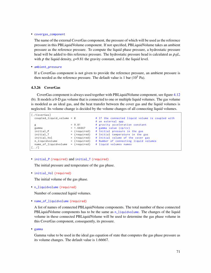
• covergas_component

The name of the external CoverGas component, the pressure of which will be used as the referencepressure in this PBLiquidVolume component. If not specified, PBLiquidVolume takes an ambientpressure as the reference pressure. To compute the liquid phase pressure, a hydrostatic pressurehead will be added to this reference pressure. The hydrostatic pressure head is calculated as ρgL,with ρ the liquid density, g=9.81 the gravity constant, and L the liquid level.

• ambient_pressure

If a CoverGas component is not given to provide the reference pressure, an ambient pressure isthen needed as the reference pressure. The default value is 1 bar (105 Pa).

4.3.26 CoverGas

CoverGas component is always used together with PBLiquidVolume component, see figure 4.12(b). It models a 0-D gas volume that is connected to one or multiple liquid volumes. The gas volumeis modeled as an ideal gas, and the heat transfer between the cover gas and the liquid volumes isneglected. Its volume change is decided by the volume changes of all connecting liquid volumes.

[./ CoverGas]coupled_liquid_volume = 0 # If the connected liquid volume is coupled with

# an external app.g = 9.81 # gravity acceleration constantgamma = 1.66667 # gamma value (cp/cv)initial_P = (required) # Initial pressure in the gasinitial_T = (required) # Initial temperature in the gasinitial_Vol = (required) # Initial volume of the cover gasn_liquidvolume = (required) # Number of connecting liquid volumesname_of_liquidvolume = (required) # liquid volumes names

[../]

• initial_P (required) and initial_T (required)

The initial pressure and temperature of the gas phase.

• initial_Vol (required)

The initial volume of the gas phase.

• n_liquidvolume (required)

Number of connected liquid volumes.

• name_of_liquidvolume (required)

A list of names of connected PBLiquidVolume components. The total number of these connectedPBLiquidVolume components has to be the same as n_liquidvolume. The changes of the liquidvolume in these connected PBLiquidVolume will be used to determine the gas phase volume inthis CoverGas component, consequently, its pressure.

• gamma

Gamma value to be used in the ideal gas equation of state that computes the gas phase pressure asits volume changes. The default value is 1.66667.

71

• coupled_liquid_volume

This input parameter specifies if the connected liquid volume is coupled with an external app. Thedefault value is false.

• g

Gravity acceleration constant. The pressure difference between the gas phase and its connectedPBLiquidVolume liquid phase is ρgL, with ρ the liquid density, g the gravity acceleration con-stant, and L the liquid level in PBLiquidVolume component.

4.3.27 PBPump

PBPump is another special junction component, and it simulates a pump, in which the pumphead can be dependent on a pre-defined function, or can be automatically adjusted to match user-specified mass flow rate. It inherits from the PBBranch component, and therefore assumes thevolume of the pump is neglectable. More complex pump models will be developed in future SAMenhancements. Pumping power can be modeled and considered in the energy conservation of thejunction.

Its input parameters are listed as follows:[./ PBPump]

Area = (required) # See PBBranchK = (required) # See PBBranchK_B = (no_default) # See PBBranchK_B_reverse = (no_default) # See PBBranchK_C = (no_default) # See PBBranchK_C_reverse = (no_default) # See PBBranchK_reverse = (no_default) # See PBBrancheos = (required) # See PBBranchinitial_P = (no_default) # See PBBranchinitial_T = (no_default) # See PBBranchinitial_V = (no_default) # See PBBranchinputs = (no_default) # See PBBranchjoint_model = 1 # See PBBranchnodal_Tbc = 0 # See PBBranchoutputs = (no_default) # See PBBranchscale_factors = '1 1 1e-06' # See PBBranch

Head = 0 # Pump headHead_fn = (no_default) # Name of the pressure head functionpump_heating = 0 # if pump heating is included in the energy conservation

Desired_mass_flow_rate = (no_default) # The desired mass flow rate of the pump.# flow rate and the desired one.

Mass_flow_rate_tolerance = 0.0001 # Relative tolerance between the pump delivered# mass flow rate and the desired one.

Response_interval = 1 # The time interval between two consecutive pump# head adjustments.

[../]

• Head

This input parameter specifies the pump head value, in [Pa]. The default value is 0.

• Head_fn

This input parameter specifies the function name to compute pump head value.

72

• pump_heating

This input parameter specifies if pump heating effect should be considered in energy balance. Thedefault is false.

• Desired_mass_flow_rate

This input parameter accepts a user-specified mass flow rate, such that the pump will automati-cally adjust the pump head to match this value. If specified, the pump head specified in the Head

input parameter is used as the initial guessing value to start with the automatical adjustment.

• Mass_flow_rate_tolerance

When a user-specified mass flow rate is given, this input parameter the absolute relative tolerancebetween the real pump mass flow rate compared with the user-specified one. If within this tol-erance, the pump stops to adjust its pump head as it is deemed that the desired mass flow ratealready achieved. The default value is 10-4.

• Response_interval

When a user-specified mass flow rate is given, this input parameter specifies the how fast, i.e., thetime internal between two consecutive pump head adjustments. The default value is 1 second.

4.3.28 StagnantVolume

StagnantVolume models a stagnant liquid volume, which has no connections to 1-D fluid com-ponents but is allowed to connect to a 0-D volume or 1-D or 2-D heat structures for heat transfer.It is assumed that there is no net mass transfer between StagnantVolume and the connecting 0-Dvolumes. Its input parameters are listed as follows:

[./ StagnantVolume]center = (required) # geometric center of the volumecoupled_volume = (no_default) # Coupled volume component nameeos = (required) # The name of equation of state object to use.height = (no_default) # Height of the componentinitial_T = (required) # initial temperature of the componentmass_flow = 0. # Function name for the exchanged flow between volumesorientation = '0 0 1' # Orientation vector of the componentposition = '0 0 0' # Origin (start) of the componentrotation = 0 # Rotation of the component (in degrees)volume = (required) # Volume of the componentwidth = (no_default) # Width of the component

[../]

• center (required)

The geometric center of the volume. It overrides the values given in position (if ever specified),and is used to generate mesh for display purpose.

• eos (required)


• initial_T (required)

The initial fluid temperature of the component.

73

• height and width

These input parameters specify the height and width of the component, both of which are to beused to generate mesh for display purpose. The default value for both parameters are 1 m.

• coupled_volume

The name of coupled volume, e.g., another StagnantVolume, which this StagnantVolume compo-nent exchanges energy with. The energy exchange between these two volumes is computed asmcp∆T , in which m is the mixing mass flow rate (see mass_flow), cp is the specific heat com-puted at the average temperature between the two mixing volume, ∆T the temperature differencebetween the two mixing volume.

• mass_flow

If a coupled volume is specified, this input parameter specifies the mixing mass flow rate betweenthe two mixing volume. It can be either a number or a function name.

• orientation, position, and rotation

Parameters not used.

4.3.29 LiquidTank

The LiquidTank component of SAM simulates a PBVolumeBranch (or PBLiquidVolume) andthe heat structure (modeled as PBCoupledHeatStructure) attached to it in order to capture this addi-tional thermal inertia. The input parameters of the LiquidTank component requires those to describethe PBVolumeBranch (or PBLiquidVolume) and those to describe the PBCoupledHeatStructure at-tached to it.

The LiquidTank component automatically create a PBLiquidVolume component, if a CoverGascomponent is connected to determine its gas phase pressure; otherwise, a PBVolumeBranch com-ponent is create. It assumes that the PBVolumeBranch (or PBLiquidVolume) is connected to theleft-side surface of PBCoupledHeatStructure, and additional boundary condition input parametersare required for the right-side surface of PBCoupledHeatStructure.

The list of input parameters are given in the following list. Part of them are required to de-scribe the PBVolumeBranch (or PBLiquidVolume) component, which could be referred to section4.3.24 (or section 4.3.25); and part of them are required to describe the PBCoupledHeatStructurecomponent, which could be referred to section 4.3.12.

[./ LiquidTank]Area = (required) # See PBVolumeBranch (PBBranch)K = (required) # See PBVolumeBranch (PBBranch)Steady = 0 # See PBVolumeBranchcenter = (required) # See PBVolumeBranchdisplay_pps = 0 # See PBVolumeBrancheos = (required) # See PBVolumeBranchheight = (no_default) # See PBVolumeBranchinitial_P = (no_default) # See PBVolumeBranch (PBBranch)initial_T = (no_default) # See PBVolumeBranch (PBBranch)initial_V = (no_default) # See PBVolumeBranch (PBBranch)inputs = (no_default) # See PBVolumeBranchrotation = 0 # See PBVolumeBranchscale_factors = '1 1 1e-06' # See PBVolumeBranchvolume = (required) # See PBVolumeBranch

74

width = (no_default) # See PBVolumeBranchnodal_Tbc = 1 # See PBVolumeBranch (PBBranch)orientation = '0 0 1' # See PBVolumeBranchoutputs = (no_default) # See PBVolumeBranchposition = '0 0 0' # See PBVolumeBranch

HS_BC_type_right = (required) # See HS_BC_type of PBCoupledHeatStructureHT_surface_area_density_right = (no_default) # See PBCoupledHeatStructureHw = (no_default) # See Hw_left of PBCoupledHeatStructureHw_right = (no_default) # See PBCoupledHeatStructureT_amb_right = 300 # See PBCoupledHeatStructureT_bc_right = 600 # See PBCoupledHeatStructureTs_init = (no_default) # See PBCoupledHeatStructuredim_hs = 2 # See PBCoupledHeatStructureelem_number_axial = 1 # See PBCoupledHeatStructureelem_number_radial = (required) # See PBCoupledHeatStructureeos_right = (no_default) # See PBCoupledHeatStructureheat_source_solid = 0 # See PBCoupledHeatStructureheat_transfer_area = (no_default) # See heat_transfer_area_left

# of PBCoupledHeatStructureheat_transfer_area_right = (no_default) # See PBCoupledHeatStructurehs_names = (no_default) # See PBCoupledHeatStructurehs_type = cylinder # See PBCoupledHeatStructurelength = (required) # See PBCoupledHeatStructurematerial_hs = (required) # See PBCoupledHeatStructurename_comp_right = (no_default) # See PBCoupledHeatStructureqs_right = (no_default) # See PBCoupledHeatStructureradius_i = (no_default) # See PBCoupledHeatStructurewidth_of_hs = (required) # See PBCoupledHeatStructure

initial_level = (no_default) # See PBLiquidVolumecovergas_component = (no_default) # See PBLiquidVolume

mesh_disp_gap = 0.1 # Axial offset for mesh generation[../]

Some details of the input parameters as discussed as follows.

• mesh_disp_gap

This input parameter specifies mesh offset in the y-direction, with respect to the fluid componentmesh, when creating heat structure meshes. The default value for this parameter is 0.1 [m]. If‘cylinder‘ is specified for hs_type, this mesh offset value will be overridden by half of radius_ivalue.

4.3.30 ReactorCore

The ReactorCore component describes a pseudo three-dimensional reactor core by connectingbypass channels to their neighboring core channels (with duct walls). Its input parameters are listedbelow.

[./ ReactorCore]n_bypasschan = (required) # Number of BypassChannelsn_corechan = (required) # Number of CoreChannelsname_of_bypasschan = (required) # BypassChannel namesname_of_corechan = (required) # CoreChannel names

[../]

• n_bypasschan (required)

75

The total number of bypass channels in this ReactorCore component.

• n_corechan (required)

The total number of core channels in this ReactorCore component.

• name_of_bypasschan (required)

The names of all bypass channels.

• name_of_corechan (required)

The names of all core channels.

4.3.31 SurfaceCoupling

The SurfaceCoupling component models the heat transfer between two solid surfaces, suitablefor radiation heat transfer or gap heat transfer between them.

[./ SurfaceCoupling]area_ratio = 1 # Area ratio between the two surfacescoupling_type = RadiationHeatTransfer(required) # Heat transfer coupling typeeos = (no_default) # The name of EOS to useepsilon_1 = 1 # Surface 1 emissivityepsilon_2 = 1 # Surface 2 emissivityh_gap = (no_default) # gap conductancelength = (no_default) # gap lengthradius_1 = (no_default) # Surface 1 radiussurface1_name = (required) # The name of the Surface 1surface2_name = (required) # The name of the Surface 2use_displaced_mesh = 1 # Whether or not this object should use the

# displaced mesh for computation.view_factor = 1 # View factor from surface master (1) to

# surface slave (2)width = (no_default) # gap width

[../]

• surface1_name (required) and surface2_name (required)

The name of surface 1 (2) that participates in the radiation or gap heat transfer.

• coupling_type (required)

The heat transfer mechanism type of the heat transfer, either ‘RadiationHeatTransfer’ for radia-tion heat transfer, or ‘GapHeatTransfer’ for gap heat transfer. The default value is ‘Radiation-HeatTransfer’.

• area_ratio

The ratio of surface 1 area to surface 2 area, which is only required for radiation heat transfer tocompute the heat flux between the two surfaces. If not specified, the default value is 1.

• radius_1

The radius of surface 1, if surface 1 is of cylindrical type.

76

• epsilon_1 and epsilon_2

The emissivity of surface 1 (2), only required for radiation heat transfer mechanism. Both param-eters have the same default value 1.

• view_factor

This parameter defines the view factor between surfaces 1 and 2, only required for radiation heattransfer mechanism. The default value is 1.

• h_gap

For gap heat transfer mechanism, if user-specified value is desired for the gap heat transfer coef-ficient, this input parameter specifies such a value. If not specified, SAM will compute the gapheat transfer coefficient from other input parameters.

• eos

The equation of state that will be used to compute gap heat transfer coefficient, only required whenthe heat transfer mechanism is gap heat transfer, and when user-specified heat transfer coefficientis not given.

• width and length

Gap width (length), only required when the heat transfer mechanism is gap heat transfer, andwhen user-specified heat transfer coefficient is not given.

• use_displaced_mesh

This parameter specifies that if displaced mesh to be used. The default value is true, and it is safeto use this default value.

4.3.32 ReactorPower

ReactorPower is a non-geometric component for describing the total reactor power, which canbe dependent on either user-defined functions (such as describing the decay heat curve), or com-puted externally from SAM’s PointKinetics component (see section 4.3.33). The total reactor powervariable is used in core components such as PBCoreChannel and PBBypassChannel.[./ ReactorPower]

decay_heat = (no_default) # Function (name) that provides decay heat curvedecay_heat_channel_name = (no_default) # Define the channel/bypass names with decay

# heat curvesinitial_power = (required) # Initial reactor powerpke = (no_default) # The name of the point kinetics component that

# computes reactor powerpoint_kinetics_power = (no_default) # Point -Kinetics model power

[../]

• initial_power (required)

This input parameter specifies the initial power of the reactor.

• decay_heat

If a decay heat curve is to be used to compute the reactor power, this input parameter specifies thedecay heat curve function name.

77

• pke

If an external PointKinetics component is to be used to compute the reactor power, this inputparameter specifies the name of the PointKinetics component.

• point_kinetics_power

If an external PointKinetics component is to be used to compute the reactor power, this inputparameter specifies the PointKinetics power.

• decay_heat_channel_name

This input parameter specifies the core channel and/or bypass channel names with decay heatcurves.

4.3.33 PointKinetics

The PointKinetics component is the build-in point kinetics model of SAM, which models thetransient behaviors of reactor fission power, delayed-neutron precursors, as well as reactivity feed-back from other components, e.g., core channels. In case of modeling molten-salt reactors, wheredrifting delayed neutron precursors effect cannot be ignored, PointKinetics component also takeaccount into the net flow in (out) effect as an additional source (sink) term. The net flow in (out)effect is captured in a coupled PBMoltenSaltChannel component.

[./ PointKinetics]Delay_neutron_precursor_name = (required) # Delay neutron precursor namesInitial_DNP_value = (no_default) # Define the initial value for delay

# neutron precursorLAMBDA = (required) # Prompt neutron lifetimeMoving_DNP_bypass_channels = (no_default) # Define the bypass channels for moving

# delay neutron precursorMoving_DNP_name = (no_default) # Define the moving delay neutron

# precursor namesNormalized_fission_power = (required) # Normalized fission power namebetai = (required) # Delay neutron fraction for group

# icore_radial_expansion_reactivity_coefficients = (no_default) # Core radial expansion

# reactivity coefficients# (delta_k / k per kg)

core_radial_expansion_reactivity_feedback = 0 # Enable core radial expansion# reactivity feedback.

core_radial_expansion_weights = (no_default) # Weights for core constraint# system on the radial expansion# reactivity.

core_radial_thermal_expansion_coefficient = (no_default) # Thermal expansion# coefficients for# core constraint system# at different locations.

coupled_radial_displacements_pps = (no_default) # coupled radial displacements for# radial expansion reactivity.

coupled_radial_temperatures_pps = (no_default) # coupled temperature for radial# expansion reactivity.

feedback_components = (no_default) # Components which have Thermal# -Hydraulics feedback on reactivity

feedback_start_time = 0 # The time that the reactivity# feedback starts.

lambda = (required) # Delay neutron precursor# decay constant

n_radial_constraint_system = (no_default) # Number of radial constraint system

78

# for core radial expansion reactivity# feedback.

rho_fn_name = (no_default) # External reactivity (delta k per# k)

use_external_radial_displacement = 0 # Enable coupled radial displacement# from external thermo -mechanical# module.

[../]

• Delay_neutron_precursor_name (required)

This input parameter specifies a list of names for delayed neutron precursors.

• Initial_DNP_value

This input parameter specifies a list of initial values for delayed neutron precursor populations.The total number of list values have to be the same as the total number of delayed neutron pre-cursor names. However, if not specified, delayed neutron precursor populations are initializedas:

Ci,initial =βi

Λλi

in which, βi is the delayed neutron precursor fraction for group i (see betai), Λ the prompt neutronlifetime (see LAMBDA), λi the delayed neutron precursor decay constant for group i (see lambda).

• LAMBDA (required)

This input parameter specifies the prompt neutron lifetime.

• lambda (required)

This input parameter specifies a list of decay constants for delayed neutron precursors. The totalnumber of list values have to be the same as the total number of delayed neutron precursor names.

• betai (required)

This input parameter specifies a list of delayed neutron precursor fractions. The total number oflist values have to be the same as the total number of delayed neutron precursor names.

• Normalized_fission_power (required)

This input parameter specifies the name of the normalized fission power variable.

• rho_fn_name

This input parameter specifies the function name to introduce an external reactivity, additional tothose from reactor feedbacks, to the PointKinetics model. If not specified, this external reactivityis 0.

• feedback_components

Besides external reactivity function, the other main reactivity feedback mechanism is thermal-hydraulics feedback from reactor core channel components. This input parameter specifies a listof components from which reactivity feedback will be computed.

79

• feedback_start_time

The time that reactor core channel components start to compute reactivity feedback. The defaultvalue is 0 second.

• core_radial_expansion_reactivity_feedback

This input parameter specifies if core radial expansion reactivity feedback should be modeled.The default value is false. If modeled, the total reactivity feedback due to core radial expansion iscomputed as,

∆Rradialexpansion =N

∑i=1

(∆LL

)iwiρi

in which,

N is the the total number of radial sections to compute reactivity feedback;see n_radial_constraint_system.

(∆L/L)i is the radial core displacement value in the i-th radial section;

wi is the weight value of the i-th radial section; see core_radial_expansion_weights.

ρi is core radial expansion coefficient at the i-th radial section;see core_radial_expansion_reactivity_coefficients.

Currently, SAM provides two ways to model core radial expansion, i.e., a simple built-in functionor coupled from external simulations. The simpler one is a built-in function, which computes thei-th radial expansion as, (

∆LL

)i= αi (Ti−T0,i)

in which,

αi is the thermal expansion coefficient of the constraint structure at the i-th radial section, seethermal_expansion_coefficient.

Ti is the core temperatures in the i-th radial section;see coupled_radial_temperatures_pps.

T0,i is the initial, i.e., when reactor core channel components start to compute reactivity feedback,core temperatures in the i-th radial section.

The radial core displacement can also be modeled from an external code, and then coupled withSAM to compute the reactivity feedback value (use_external_radial_displacement = true).

• use_external_radial_displacement

This input parameter specifies if core radial displacement should be modeled from an externalsimulation and their values are provided as coupled values. The default value is false. If specifiedtrue, externally computed core radial expansion displacement is expected from user input, seecoupled_radial_displacements_pps.

80

• n_radial_constraint_system

If core radial expansion reactivity feedback is modeled, this input parameter specifies the numberof radial constraint system, i.e., number of core radial sections, for core radial expansion reactivityfeedback.

• core_radial_expansion_reactivity_coefficients

This input parameter specifies a list of core radial expansion reactivity feedback coefficient values.The total number of this list of values has to be the same as the number of core radial sections(see n_radial_constraint_system).

• core_radial_expansion_weights

This input parameter specifies a list of values for core radial expansion reactivity feedback weights.The total number of this list of values has to be the same as the number of core radial sections(see n_radial_constraint_system).

• thermal_expansion_coefficient

If radial expansion is modeled used SAM’s built-in function, this input parameter specifies alist of thermal expansion coefficients to compute radial core displacement values. The totalnumber of this list of values has to be the same as the number of core radial sections (seen_radial_constraint_system).

• coupled_radial_temperatures_pps

If radial expansion is modeled used SAM’s built-in function, this input parameter specifies alist of Postprocessor names that compute core temperatures in each radial section. The to-tal number of this list of names has to be the same as the number of core radial sections (seen_radial_constraint_system).

• coupled_radial_displacements_pps

If core radial displacement should be modeled from an external simulation and their values areprovided as coupled values, this input parameter specifies a list of Postprocessor names that com-pute core radial displacement at each radial section. The total number of this list of names has tobe the same as the number of core radial sections (see n_radial_constraint_system).

• Moving_DNP_bypass_channels

If drifting delayed neutron precursors effect should be considered, this input parameter specifiesthe PBMoltenSaltChannel component name, from which the net flow in (out) of drifting delayedneutron precursors are computed.

• Moving_DNP_name

If drifting delayed neutron precursors effect should be considered, this input parameter specifiesthe names of these delayed neutron precursors.

81

4.3.34 ReferenceBoundary

ReferenceBoundary component provides a fixed value boundary condition to a one-dimensionalfluid type of component. This boundary condition can be applied to normal flow parameters, suchas pressure, velocity, and temperature, as well as scalar variables.

[./ ReferenceBoundary]coupled_var = (no_default) # coupled variable at bcinput = (no_default) # Names of the connected componentsvalue = (no_default) # Given variable value on boundaryvariable = (required) # variable to be set at bc

[../]

• input

This input parameter specifies where this boundary condition should be applied, e.g., input =

'pipe-1(in)'.

• variable (required)

This input parameter specifies which variable this boundary condition should be applied, e.g.,variable = pressure. In principle, this can be any field variable, but pressure is commonly usedto setup the system reference pressure.

• value

This input parameter specifies the value to be applied to the variable in this boundary condition.

• coupled_var

This input parameter specifies a coupled variable, whose value is to be applied to the variable inthis boundary condition.

4.3.35 PipeChain

PipeChain is a non-geometric component for sequentially connecting a number of fluid compo-nents. It automatically generates the needed PBSingleJunction components between the specifiedfluid components. The purpose of this component for user friendliness.

There are only two input parameters required for this component:

• eos (required)

Equation of state to be used for all automatically-generated PBSingleJunctions.

• component_names

This input parameter specifies a list of N sequentially connected fluid components, and N − 1PBSingleJunctions will be automatically generated to connect them.

4.3.36 ChannelCoupling

ChannelCoupling is a non-geometric component for coupling two 1-D fluid components (withenergy exchange). It is intended to model the flow mixing between two parallel channels.

82

[./ ChannelCoupling]beta = (required) # turbulent mixing parametereos = (required) # The name of EOS to usegap_width = (required) # The gap widthpipe1_name = (no_default) # The name of the Pipe 1pipe2_name = (no_default) # The name of the Pipe 2var_scaling_factor = 0.001 # turbulent mixing flux variable scaling factor

[../]

• pipe1_name and pipe2_name

The names of the two pipes where this flow mixing is happening.

• eos (required)

Equation of state to be used in this ChannelCoupling component.

• gap_width (required)

Gap width between the two pipes where this flow mixing is happening.

• beta (required)

This input parameter specifies the turbulent mixing coefficient value to be used to compute theinter-channel mass flux due to turbulent mixing, which will then be used to compute the inter-channel energy flux due to turbulent mixing.

• var_scaling_factor

This input parameter specifies the scaling factor for the variable for computing the inter-channelmass flux due to turbulent mixing.

4.3.37 HeatPipe and HeatPipeArray

Both components are currently under development, which will be included in future versions ofthis user’s guide.

4.4 ComponentInputParameters

Independent to the [Components] input block, SAM also provides a separate [ComponentInput-

Parameters] input block, where users could provide input template for certain types of SAM com-ponents. Note that this input block only provides component ‘template’, and by itself, no realcomponents will created. There are two common usages of this input block: 1) to provide the com-mon features of a type of component, which will be used as reference to build real components inthe [Components] input block; and 2) to provide a completely predefined component that will bereferred to and created as a sub-component of a composite-type of component. The two commonusages are to be discussed in the remaining part of this section. Currently, the SAM componentsthat supports such a feature is listed in Table 4.1.

The first usage is to provide common features for components input. When preparing SAMinput files to perform thermal-hydraulics analysis, it is typical to observe that many componentsshare common features, for example, a test loop with the majority of it built from a type of standard

83

Table 4.1: SAM components that supports ComponentInputParameters feature

ComponentInputParameters SAM Component NameDuctedFuelAssemblyParameters DuctedFuelAssemblyHeatPipeParameters HeatPipeHeatStructureParameters HeatStructureMultiChannelRodBundleParameters MultiChannelRodBundlePBCoreChannelParameters PBCoreChannelPBOneDFluidComponentParameters PBOneDFluidComponentPBPipeParameters PBPipe

ASME pipe. In this case, [ComponentInputParameters] can be used to provide the abstracted com-mon features of such a type of components, and [Components] only provides component-specificparameters and refers to these common features to generate the complete input parameter list.With this approach, it greatly reduces users’ burden to type in the same parameters for manytimes, and also reduces the possibility of input error. Note that input parameters specified in the[Components] input blocks can override what has been provided as common features provided inthe [ComponentInputParameters] input block. An example is given as follows:

[ComponentInputParameters]# This sub -block provides component input parameter with common features[./ Schedule -10-w-insulation]

type = PBPipeParameterseos = eosA = 6.097763E-04heat_source = 0Dh = 2.786380E-02hs_type = cylinderTwall_init = 2.981500E+02heat_source_solid = '0 0'dim_wall = 2wall_thickness = '0.0027686 0.0508 'n_wall_elems = '2 4'material_wall = 'SS -304 Fiberglass 'HS_BC_type = TemperatureT_wall = 2.981500E+02HT_surface_area_density = 355.5 # This parameter will be overridden

# in one of the two components[../]

[]

[Components][./pipe -1]

type = PBPipeinput_parameters = Schedule -10-w-insulation # This refers to the PBPipeParameters

# with common featureslength = 1position = '0 0 0'orientation = '1 0 0'n_elems = 20initial_V = -0.1

[../]

[./pipe -2]type = PBPipeinput_parameters = Schedule -10-w-insulation # This refers to the PBPipeParameters

84

# with common featureslength = 2position = '1 0 0'orientation = '0 0 1'n_elems = 25initial_V = -0.1HT_surface_area_density = 100.0 # This parameter overrides what has been

# provided in Schedule -10-w-insulation[../]

[]

The other usage is to provide needed input parameters, which predefines a component that willbe referred to and created as a sub-component of a composite-type of component. Currently, thisonly happens to a special component, HexLatticeCore, which relies on several predefined compo-nents to create its sub-components (see section 4.3.11 for more details). An example is given asfollows:[ComponentInputParameters]

[./F1] # Predefined PBCoreChanneltype = PBCoreChannelParameterseos = eosA = 0.005105685Dh = 0.003446961length = 0.8n_elems = 20HT_surface_area_density = 1068.182718dim_hs = 2name_of_hs = 'fuel gap clad'Ts_init = 628.15n_heatstruct = 3fuel_type = cylinderwidth_of_hs = '0.003015 0.000465 0.00052 'elem_number_of_hs = '5 1 1'material_hs = 'fuel -mat gap -mat clad -mat'power_shape_function = ppf_axial

[../]

[./ reference_hs] # Predefined heat strucutres for intra -assembly duct walls and gaptype = HeatStructureParametershs_type = platelength = 0.8dim_hs = 2elem_number_axial = 20elem_number_radial = '2 2 2'width_of_hs = '0.003 0.004 0.003 'material_hs = 'duct -mat gap -mat duct -mat'hs_names = 'duct_i gap duct_o 'Ts_init = 628.15HS_BC_type = 'Coupled Coupled 'eos_left = eoseos_right = eosHT_surface_area_density_left = 15.3766HT_surface_area_density_right = 15.3766

[../]

[./ duct_wall] # Predefined heat strucutres for duct walltype = HeatStructureParametershs_type = platelength = 0.8dim_hs = 2elem_number_axial = 20elem_number_radial = 2width_of_hs = '0.003 '

85

material_hs = 'duct -mat'hs_names = 'duct'Ts_init = 628.15eos_left = eosHS_BC_type = 'Coupled Adiabatic 'HT_surface_area_density_left = 15.3766

[../][]

[Components][./ core]

type = HexLatticeCoreposition = '0 0 0'orientation = '0 0 1'n_side = 2assem_pitch = 0.14598assem_Dft = 0.13598radial_power_peaking = '1 1 1 1.5 1 1 0.5'

assem_layout = 'F1 F1 F1 F1 F1 F1 F1' # F1 refers to the predefined# PBCoreChannelParameters

ref_hs = reference_hs # This refers to a predefined heat structureref_duct = duct_wall # This refers to a predefined duct wall heat structure

[../][]

4.5 PostProcessors

4.5.1 ComponentBoundaryEnergyBalance

This Postprocessor is designed to monitor the energy flux balance between two selected pipeends. A common usage is to monitor the energy balance of a pipe component on its two ends, andcompare it with the total heat source applied to this pipe.

[./ ComponentBoundaryEnergyBalance]eos = (required) # The name of equation of state object to use.execute_on = TIMESTEP_END # The list of flag(s) indicating when this object should

# be executed , the available options include NONE , INITIAL ,# LINEAR , NONLINEAR , TIMESTEP_END ,# TIMESTEP_BEGIN , FINAL , CUSTOM.

input = (required) # Name of the components and boundaries[../]

• input (required)

This input parameter specifies a list of two pipe ends, where energy fluxes are to be compared tocompute an energy balance between them:

(ρuhA)2− (ρuhA)1 .

The input syntax is similar to those for junction type of component, e.g., input = 'pipe-1(in)

pipe-1(out)' or input = 'IHX(secondary_in) IHX(secondary_out)'.

• eos (required)

Equation of state used in the pipe component.

86

• execute_on

This is an input parameter inherited from MOOSE framework, it specifies how often this Postpro-cessor should perform a computation. It is common to all Postprocessors to be discussed in thissection, and in general, it is safe to not specify anything.

4.5.2 ComponentBoundaryFlow

This Postprocessor is simply monitors the mass flow rate, ρuA, of a pipe end.

[./ ComponentBoundaryFlow]input = (required) # Name of the components and boundariesscale_factor = 1 # Scale factor to be applied to the ordinate values

[../]


This input parameter specifies a pipe and one of its ends, where mass flow rate is to be com-puted as ρuA. The input syntax is similar to those for junction type of component, e.g., input =

pump_pipe(in).

• scale_factor

This is a scaling factor to be multiplied to the mass flow rate. The default value is 1.

4.5.3 ComponentBoundaryScalarFlow

This Postprocessor is similar to ComponentBoundaryFlow, and it simply monitors the flow rateof a passive scalar, ρuAφ , of a pipe end.

[./ ComponentBoundaryScalarFlow]input = (required) # Name of the components and boundariesvariable = (required) # Name of the particlescale_factor = 1 # Scale factor to be applied to the ordinate values

[../]


This input parameter specifies a pipe and one of its ends, where the flow rate of a passive scalaris to be computed as ρuAφ . The input syntax is similar to those for junction type of component,e.g., input = pump_pipe(in).


The name of the passive scalar variable.

• scale_factor

This is a scaling factor to be multiplied to the flow rate of the passive scalar. The default value is1.

87

4.5.4 ComponentBoundaryVariableValue

This Postprocessor returns the value of a specified variable at a pipe end.[./ ComponentBoundaryVariableValue]

input = (required) # Name of the components and boundariesvariable = (required) # Name of the variablescale_factor = 1 # Scale factor to be applied to the ordinate values

[../]


The same as in ComponentBoundaryScalarFlow.


The name of the variable, such as “pressure”, “temperature”, “velocity”, “rho” (fluid density),“enthalpy”, “heat˙transfer˙coefficient” (if modeled), and passive scalars (if modeled).

• scale_factor

This is a scaling factor to be multiplied to the variable value. The default value is 1.

4.5.5 ComponentNodalVariableValue

This Postprocessor returns the value of a specified variable on a specified node in a pipe.[./ ComponentNodalVariableValue]

input = (required) # Name of the components and boundariesvariable = (required) # Name of the variablescale_factor = 1 # Scale factor to be applied to the ordinate values

[../]


This input parameter specifies a pipe and a node id, where the value of the specified variable willbe returned. The input syntax is, for example, input = pipe(0) or input = IHX:primary_pipe(10).Note that node id starts from 0.


The same as in ComponentBoundaryVariableValue.

• scale_factor

This is a scaling factor to be multiplied to the variable value. The default value is 1.

4.5.6 ConductionHeatRemovalRate

This Postprocessor computes the integral heat removal rate from a side of a two-dimensionalheat structure.[./ ConductionHeatRemovalRate]

boundary = (required) # The list of boundary IDs from# the mesh where this boundary# condition applies

heated_perimeter = (required) # The length of the HeatExchanger heated perimeter[../]

88

• boundary (required)

This input parameter specifies the boundary name where the integral heat removal rate to becomputed, for example, boundary = ’hp0:cond_wall’.

• heated_perimeter (required)

The heated perimeter of the boundary to compute the integral heat removal rate,

Q =∫−k∇T PhdL

in which, −k∇T is the local surface heat flux, dL is the length along the boundary side, and Ph isthis heated perimeter input parameter.

4.5.7 HeatExchangerHeatRemovalRate

This Postprocessor computes the integral heat removal rate from the wall heat structure of a heatexchanger to a specified pipe, e.g., the primary or the secondary side pipe.

[./ HeatExchangerHeatRemovalRate]block = (required) # The list of block ids (SubdomainID)

# that this object will be appliedheated_perimeter = (required) # The length of the HeatExchanger heated perimeter

[../]

• block (required)

This input parameter specifies the block name where the integral heat removal rate to be com-puted, for example, block = 'DHX:primary_pipe'.

• heated_perimeter (required)

The heated perimeter of the boundary to compute the integral heat removal rate,

Q =∫

h(Tf −Twall)PhdL

in which, h is the local heat transfer coefficient, Tf is the local fluid temperature, Twall is the localwall surface temperature, dL is the length along the pipe, and Ph is this heated perimeter inputparameter.

4.6 TimeSteppers

4.6.1 CourantNumberTimeStepper

The CourantNumberTimeStepper is a TimeStepper inherited from PostprocessorDT, which com-putes time step size based on a Postprocessor value, in this case, MaxCourantNumber. Its inputparameters are listed as follows:

[./< CourantNumberTimeStepper >]Courant_number = 10 # Target Courant numberdt = (no_default) # Initial value of dtfactor = 0 # Add a factor to the

# supplied postprocessor

89

# value.postprocessor = Simulation:MaxCourantNumber(required) # The name of the postprocessor

# that computes the dtreset_dt = 0 # Use when restarting

# a calculation to force# a change in dt.

scale = 1 # Multiple scale and# supplied postprocessor# value.

type = CourantNumberTimeStepper[../]

Input parameters are discussed as follows:

• Courant_number

This TimeStepper adjusts the time step size to match this given Courant number as a userinput parameter. The default value is 10.

• dt

The initial value of time step size for this TimeStepper to start with. If not specified, the codeuses a default value of 0.01 second.

• factor and scale

These two input parameters are not used.

• postprocessor

You do NOT and should NOT specify this input parameter. A default value, Simulation:MaxCourantNumber, has been automatically generated and given to this parameter.

• reset_dt (advanced MOOSE option)

Use when restarting a calculation to force a change in dt. By default, it is false (0).

An example input of the CourantNumberTimeStepper block is shown below.

[./ TimeStepper]type = CourantNumberTimeStepperdt = 0.02Courant_number = 0.5

[../]

This input block should be used as an sub-block of the Executioner input block.

4.7 Preconditioning

The Preconditioning block describes the preconditioner to be used by the preconditioned JFNKsolver (available through PETSc). Two options are currently available, the single matrix precondi-tioner (SMP) and the finite difference preconditioner (FDP). The FDP option uses numerical Jaco-bian by doing direct finite differences of the residual terms. It is normally slow, and only intendedfor debugging purposes. The SMP option is more efficient and the recommended option. The inputparameters of the Preconditioning block are shown below. An example input block follows.

90

[Preconditioning][./*]

active = __all__ # If specified only the blocks named will be# visited and made active

line_search = default # Specifies the line search type (Note:# none = basic)

petsc_options = # Singleton PETSc optionspetsc_options_iname = # Names of PETSc name/value pairspetsc_options_value = # Values of PETSc name/value pairs (must

# correspond with "petsc_options_iname"solve_type = # PJFNK: Preconditioned Jacobian -Free Newton

# Krylov JFNK , NEWTON , FD, LINEAR[../]

[./ FDP]control_tags = # Adds user -defined labels for accessing

# object parameters via control logic.enable = 1 # Set the enabled status of the MooseObject.full = 0 # Set to true if you want the full set of

# couplings.implicit_geometric_coupling = 0 # Set to true if you want to add entries into

# the matrix for degrees of freedom that might# be coupled by inspection of the geometric# search objects.

line_search = default # Specifies the line search type (Note:# none = basic)

off_diag_column = # The off diagonal column you want to add into# the matrix , it will be associated with an# off diagonal row from the same position in# off_diag_row.

off_diag_row = # The off diagonal row you want to add into# the matrix , it will be associated# with an off diagonal column from the same# position in off_diag_colum.

pc_side = right # Preconditioning sidepetsc_options = # Singleton PETSc optionspetsc_options_iname = # Names of PETSc name/value pairspetsc_options_value = # Values of PETSc name/value pairs (must


# Krylov JFNK , NEWTON , FD, LINEARtype = FDP

[../]

[./ SMP]control_tags = # Adds user -defined labels for accessing

# object parameters via control logic.coupled_groups = # List multiple space separated groups of

# comma separated variables. Off -diagonal# jacobians will be generated for all pairs# within a group.

enable = 1 # Set the enabled status of the MooseObject.full = 0 # Set to true if you want the full set of

# couplings.line_search = default # Specifies the line search type (Note:

# none = basic)off_diag_column = # The off diagonal column you want to add into

# the matrix , it will be associated with an# off diagonal row from the same position in# off_diag_row.

off_diag_row = # The off diagonal row you want to add into# the matrix , it will be associated# with an off diagonal column from the same

91

# position in off_diag_colum.pc_side = right # Preconditioning sidepetsc_options = # Singleton PETSc optionspetsc_options_iname = # Names of PETSc name/value pairspetsc_options_value = # Values of PETSc name/value pairs (must


# Krylov JFNK , NEWTON , FD, LINEARtype = SMP

[../][]

[Preconditioning]active = 'SMP_PJFNK '

[./ SMP_PJFNK]type = SMP # Single -Matrix Preconditionerfull = true # Using the full set of couplings among all variablessolve_type = 'PJFNK ' # Using Preconditioned JFNK solution methodpetsc_options_iname = '-pc_type ' # Names of PETSc name/value pairspetsc_options_value = 'lu' # Values of PETSc name/value pairs

[../]

[]

4.8 Executioner

The Executioner block describes the calculation process flow used in the simulation. The com-mon MOOSE Executioners are also listed here, and the associated input parameters of the Execu-tioner block are shown below. An example of the Executioner input block is also followed. Com-mon SAM MOOSE Executioner types include: CoupledCFDExecutioner (for coupled simulationwith CFD codes), CoupledSASTransient (for coupled SAS/SAM transient simulations), Steady (forsteady state simulation), and Transient (for transient simulations).[./< Executioner >][Executioner]

active = __all__ # If specified only the blocks named will be# visited and made active

petsc_options_iname = # petsc options namespetsc_options_value = # petsc options valuesscheme = bdf2 # Time integration scheme used.

[./<type >][./ CoupledCFDExecutioner]

CFD_scaling_factor = 1 # the scaling factor in the CFD modelSYSCFDBoundaryConsistency = (required) # if the SYS and CFD Boundaries are

# consistentabort_on_solve_fail = 0 # abort if solve not converged rather than

# cut timestepcompute_initial_residual_before_preset_bcs = 0 # Use the residual norm computed

# *before* PresetBCs are imposed in relative# convergence check

control_tags = # Adds user -defined labels for accessing# object parameters via control logic.

dt = 1 # The timestep size between solvesdtmax = 1e+30 # The maximum timestep size in an adaptive rundtmin = 2e-14 # The minimum timestep size in an adaptive runenable = 1 # Set the enabled status of the MooseObject.end_time = 1e+30 # The end time of the simulationinput_data_file = (required) # Input data file from external coupling

92

isRestarting = 0 # if it is a restart coupled code simulationl_abs_step_tol = -1 # Linear Absolute Step Tolerancel_max_its = 10000 # Max Linear Iterationsl_tol = 1e-05 # Linear Toleranceline_search = default # Specifies the line search type

# (Note: none = basic)n_in_parameter = (required) # Number of coupling input parametersn_out_parameter = (required) # Number of coupling output parametersn_startup_steps = 0 # The number of timesteps during startupname_of_in_components = (required) # Names of coupling input componentsname_of_in_parameters = (required) # Parameter names of coupling input

# componentsname_of_out_components = (required) # Names of coupling output componentsname_of_out_parameters = (required) # Variable names of coupling output

# componentsnames_of_CFD_boundary = (required) # names of coupled CFD boundariesnl_abs_step_tol = 1e-50 # Nonlinear Absolute step Tolerancenl_abs_tol = 1e-50 # Nonlinear Absolute Tolerancenl_max_funcs = 10000 # Max Nonlinear solver function evaluationsnl_max_its = 50 # Max Nonlinear Iterationsnl_rel_step_tol = 1e-50 # Nonlinear Relative step Tolerancenl_rel_tol = 1e-08 # Nonlinear Relative Toleranceno_fe_reinit = 0 # Specifies whether or not to reinitialize

# FEsnum_steps = 4294967295 # The number of timesteps in a transient runoutput_data_file = (required) # Output data file for external couplingpetsc_options = # Singleton PETSc optionspetsc_options_iname = # Names of PETSc name/value pairspetsc_options_value = # Values of PETSc name/value pairs (must

# correspond with "petsc_options_iname"picard_abs_tol = 1e-50 # The absolute nonlinear residual to shoot

# for during Picard iterations. This check is# performed based on the Master app's# nonlinear residual.

picard_max_its = 1 # Number of times each timestep will be# solved. Mainly used when wanting to do# Picard iterations with MultiApps that# are set to execute_on# timestep_end or timestep_begin

picard_rel_tol = 1e-08 # The relative nonlinear residual drop# to shoot for during Picard iterations.# This check is performed based on the Master# app's nonlinear residual.

reset_dt = 0 # Use when restarting a calculation to force# a change in dt.

restart_file_base = # File base name used for restartscheme = # Time integration scheme used.solve_type = # PJFNK: Preconditioned Jacobian -Free Newton

# Krylov JFNK , NEWTON , FD, LINEARsplitting = # Top -level splitting defining a hierarchical

# decomposition into subsystems to help# the solver.

ss_check_tol = 1e-08 # Whenever the relative residual changes by# less than this the solution# will be considered to be at steady state.

ss_tmin = 0 # Minimum number of timesteps to take before# checking for steady state conditions.

start_time = 0 # The start time of the simulationtime_period_ends = # The end times of time periodstime_period_starts = # The start times of time periodstime_periods = # The names of periodstimestep_tolerance = 2e-14 # the tolerance setting for final timestep

# size and sync timestrans_ss_check = 0 # Whether or not to check for steady state

93

# conditionstype = CoupledCFDExecutioneruse_multiapp_dt = 0 # If true then the dt for the simulation will

# be chosen by the MultiApps. If false# (the default) then the minimum over the# master dt and the MultiApps is used

verbose = 0 # Print detailed diagnostics on timestep# calculation

[../]

[./ CoupledSASTransient]abort_on_solve_fail = 0 # abort if solve not converged rather than

# cut timestepcompute_initial_residual_before_preset_bcs = 0 # Use the residual norm computed

# *before* PresetBCs are imposed in relative# convergence check


coupling_components = (required) # Names of coupling componentsdt = 1 # The timestep size between solvesdtmax = 1e+30 # The maximum timestep size in an adaptive rundtmin = 2e-14 # The minimum timestep size in an adaptive runenable = 1 # Set the enabled status of the MooseObject.end_time = 1e+30 # The end time of the simulationinput_fifo = (required) # Input data named pipe from external

# couplingl_abs_step_tol = -1 # Linear Absolute Step Tolerancel_max_its = 10000 # Max Linear Iterationsl_tol = 1e-05 # Linear Toleranceline_search = default # Specifies the line search type

# (Note: none = basic)n_startup_steps = 0 # The number of timesteps during startupnl_abs_step_tol = 1e-50 # Nonlinear Absolute step Tolerancenl_abs_tol = 1e-50 # Nonlinear Absolute Tolerancenl_max_funcs = 10000 # Max Nonlinear solver function evaluationsnl_max_its = 50 # Max Nonlinear Iterationsnl_rel_step_tol = 1e-50 # Nonlinear Relative step Tolerancenl_rel_tol = 1e-08 # Nonlinear Relative Toleranceno_fe_reinit = 0 # Specifies whether or not to reinitialize

# FEsnum_steps = 4294967295 # The number of timesteps in a transient runoutput_fifo = (required) # Output data named pipe from external

# couplingpetsc_options = # Singleton PETSc optionspetsc_options_iname = # Names of PETSc name/value pairspetsc_options_value = # Values of PETSc name/value pairs (must






restart_file_base = # File base name used for restartscheme = # Time integration scheme used.

94

solve_type = # PJFNK: Preconditioned Jacobian -Free Newton# Krylov JFNK , NEWTON , FD, LINEAR

splitting = # Top -level splitting defining a hierarchical# decomposition into subsystems to help# the solver.





# conditionstype = CoupledSASTransientuse_multiapp_dt = 0 # If true then the dt for the simulation will



[../]

[./ Steady]compute_initial_residual_before_preset_bcs = 0

# Use the residual norm computed *before*# PresetBCs are imposed in relative# convergence check


enable = 1 # Set the enabled status of the MooseObject.l_abs_step_tol = -1 # Linear Absolute Step Tolerancel_max_its = 10000 # Max Linear Iterationsl_tol = 1e-05 # Linear Toleranceline_search = default # Specifies the line search type

# (Note: none = basic)nl_abs_step_tol = 1e-50 # Nonlinear Absolute step Tolerancenl_abs_tol = 1e-50 # Nonlinear Absolute Tolerancenl_max_funcs = 10000 # Max Nonlinear solver function evaluationsnl_max_its = 50 # Max Nonlinear Iterationsnl_rel_step_tol = 1e-50 # Nonlinear Relative step Tolerancenl_rel_tol = 1e-08 # Nonlinear Relative Toleranceno_fe_reinit = 0 # Specifies whether or not to reinitialize

# FEspetsc_options = # Singleton PETSc optionspetsc_options_iname = # Names of PETSc name/value pairspetsc_options_value = # Values of PETSc name/value pairs (must

# correspond with "petsc_options_iname"restart_file_base = # File base name used for restartsolve_type = # PJFNK: Preconditioned Jacobian -Free Newton



type = Steady[../]

[./ Transient]abort_on_solve_fail = 0 # abort if solve not converged rather than

# cut timestep

95


dt = 1 # The timestep size between solvesdtmax = 1e+30 # The maximum timestep size in an adaptive rundtmin = 2e-14 # The minimum timestep size in an adaptive runenable = 1 # Set the enabled status of the MooseObject.end_time = 1e+30 # The end time of the simulation

l_abs_step_tol = -1 # Linear Absolute Step Tolerancel_max_its = 10000 # Max Linear Iterationsl_tol = 1e-05 # Linear Toleranceline_search = default # Specifies the line search type

# (Note: none = basic)n_startup_steps = 0 # The number of timesteps during startupnl_abs_step_tol = 1e-50 # Nonlinear Absolute step Tolerancenl_abs_tol = 1e-50 # Nonlinear Absolute Tolerancenl_max_funcs = 10000 # Max Nonlinear solver function evaluationsnl_max_its = 50 # Max Nonlinear Iterationsnl_rel_step_tol = 1e-50 # Nonlinear Relative step Tolerancenl_rel_tol = 1e-08 # Nonlinear Relative Toleranceno_fe_reinit = 0 # Specifies whether or not to reinitialize

# FEsnum_steps = 4294967295 # The number of timesteps in a transient runpetsc_options = # Singleton PETSc optionspetsc_options_iname = # Names of PETSc name/value pairspetsc_options_value = # Values of PETSc name/value pairs (must






restart_file_base = # File base name used for restartscheme = # Time integration scheme used.solve_type = # PJFNK: Preconditioned Jacobian -Free Newton







# conditionstype = Transientuse_multiapp_dt = 0 # If true then the dt for the simulation will

96



[../]

[./ Quadrature]active = __all__ # If specified only the blocks named will be

# visited and made activeelement_order = AUTO # Order of the quadrature for elementsorder = AUTO # Order of the quadratureside_order = AUTO # Order of the quadrature for sidestype = GAUSS # Type of the quadrature rule

[../]

[./ TimeStepper]active = __all__ # If specified only the blocks named will be

# visited and made active[./<type >]

[./ ContinueOnDtMinTimeStepper]control_tags = # Adds user -defined labels for accessing

# objectparameters via control logic.enable = 1 # Set the enabled status of the MooseObject.growth_factor = 2 # Maximum ratio of new to previous timestep

# sizes following a step that required the# time step to be cut due to a failed solve.

interpolate = 1 # Whether or not to interpolate DT between# times. This is true by default for# historical reasons.

min_dt = 0 # The minimal dt to take.reset_dt = 0 # Use when restarting a calculation to force

# a change in dt.time_dt = # The values of dttime_t = # The values of ttype = ContinueOnDtMinTimeStepper

[../]

[./ CourantNumberTimeStepper]Courant_number = 10 # Target Courant numbercontrol_tags = # Adds user -defined labels for accessing

# object parameters via control logic.dt = # Initial value of dtenable = 1 # Set the enabled status of the MooseObject.postprocessor = Simulation:MaxCourantNumber

# The name of the postprocessor that# computes the dt


type = CourantNumberTimeStepper[../]

[./ FunctionDT]control_tags = # Adds user -defined labels for accessing

# object parameters via control logic.enable = 1 # Set the enabled status of the MooseObject.growth_factor = 2 # Maximum ratio of new to previous timestep

# sizes following a step that required the# time step to be cut due to a failed solve.

interpolate = 1 # Whether or not to interpolate DT between# times. This is true by default for# historical reasons.

min_dt = 0 # The minimal dt to take.reset_dt = 0 # Use when restarting a calculation to force

97

# a change in dt.time_dt = # The values of dttime_t = # The values of ttype = FunctionDT

[../]

[./ PostprocessorDT]control_tags = # Adds user -defined labels for accessing

# object parameters via control logic.dt = # Initial value of dtenable = 1 # Set the enabled status of the MooseObject.postprocessor = (required) # The name of the postprocessor that computes

# the dtreset_dt = 0 # Use when restarting a calculation to force

# a change in dt.type = PostprocessorDT

[../][../]

[../][]

[../]

[Executioner]type = Transient # This is a transient simulation

dt = 1e-1 # Targeted time step sizedtmin = 1e-10 # The allowed minimum time step size

petsc_options_iname = '-ksp_gmres_restart ' # Additional PETSc settings , name listpetsc_options_value = '300' # Additional PETSc settings , value list

nl_rel_tol = 1e-7 # Relative nonlinear tolerance for each Newton solvenl_abs_tol = 1e-6 # Relative nonlinear tolerance for each Newton solvenl_max_its = 30 # Number of nonlinear iterations for each Newton solve

l_tol = 1e-6 # Relative linear tolerance for each Krylov solvel_max_its = 100 # Number of linear iterations for each Krylov solve

start_time = 0.0 # Physical time at the beginning of the simulationnum_steps = 100 # Max. simulation time stepsend_time = 100. # Max. physical time at the end of the simulation

[./ Quadrature]type = TRAP # Using trapezoid integration ruleorder = FIRST # Order of the quadrature

[../][]

4.9 Outputs

The Outputs block specifies various settings of different output types (screen display and files)in the simulation. The input parameters of common MOOSE Outputs are shown below, with anexample Outputs block followed. Common MOOSE output types include:

• CSV: write post-processor and scalar variables to a separate comma-separated-values file,

• Checkpoint: save snapshots of the simulation data including all meshes, solutions, and statefulobject data,

98

• Console: output to screen with runtime information,

• Exocdus: write all mesh and solution data to an ExodusII file.

[Outputs]active = __all__ # If specified only the blocks named will be

# visited and made active[./ CSV]

additional_execute_on = # This list of output flags is added to the# existing flags (initial|linear|nonlinear|# timestep_end|timestep_begin|final|# failed|custom)# to execute only at that moment

align = 0 # Align the outputted csv data by padding# the numbers with trailing whitespace

append_date = 0 # When true the date and time are appended# to the output filename.

append_date_format = # The format of the date/time to append ,# if not given UTC format used (see# http ://www.cplusplus.com/reference# /ctime/strftime ).

append_restart = 0 # Append existing file on restartcontrol_tags = # Adds user -defined labels for accessing

# object parameters via control logic.delimiter = # Assign the delimiter (default is ','enable = 1 # Set the enabled status of the MooseObject.end_time = # Time at which this output object stop

# operatingexecute_elemental_variables = 1 # Enable/disable the output of elemental

# variablesexecute_input = 1 # Enable/disable the output of input file

# informationexecute_nodal_variables = 1 # Enable/disable the output of nodal

# variablesexecute_on = 'INITIAL TIMESTEP_END ' # Set to

# (none|initial|linear|nonlinear|# timestep_end|timestep_begin|final|# failed|custom)# to execute only at that moment

execute_postprocessors_on = # Control of when postprocessors are outputexecute_scalar_variables = 1 # Enable/disable the output of aux scalar

# variablesexecute_scalars_on = # Control the output of scalar variablesexecute_system_information = 1 # Enable/disable the output of the simulation

# informationexecute_vector_postprocessors = 1 # Enable/disable the output of vector

# postprocessorsexecute_vector_postprocessors_on = # Enable/disable the output of

#VectorPostprocessorsfile_base = # The desired solution output name without an

# extensionhide = # A list of the variables and postprocessors

# that should NOT be output to the Exodus# file (may include Variables ,# ScalarVariables , and Postprocessor names).

interval = 1 # The interval at which time steps are output# to the solution file

linear_residual_dt_divisor = 1000 # Number of divisions applied to time step# when outputting linear residuals

linear_residual_end_time = # Specifies an end time to begin output on# each linear residual evaluation

linear_residual_start_time = # Specifies a start time to begin output on# each linear residual evaluation

99

linear_residuals = 0 # Specifies whether output occurs on each# linear residual evaluation

nonlinear_residual_dt_divisor = 1000 # Number of divisions applied to time step# when outputting non -linear residuals

nonlinear_residual_end_time = # Specifies an end time to begin output on# each nonlinear residual evaluation

nonlinear_residual_start_time = # Specifies a start time to begin output on# each nonlinear residual evaluation

nonlinear_residuals = 0 # Specifies whether output occurs on each# nonlinear residual evaluation

output_if_base_contains = # If this is supplied then output will only# be done in the case that the output base# contains one of these strings. This is# helpful in outputting only a subset of# outputs when using MultiApps.

output_linear = 0 # Specifies whether output occurs on each# linear residual evaluation

output_nonlinear = 0 # Specifies whether output occurs on each# nonlinear residual evaluation

output_postprocessors = 1 # Enable/disable the output of postprocessorsprecision = 14 # Set the output precisionshow = # A list of the variables and postprocessors

# that should be output to the Exodus file# (may include Variables , ScalarVariables ,# and Postprocessor names).

start_time = # Time at which this output object begins to# operate

sync_only = 0 # Only export results at sync timessync_times = # Times at which the output and solution is

# forced to occurtime_data = 0 # When true and VecptorPostprocessor data

# exists , write a csv file containing# the timestep and time information.

time_tolerance = 1e-14 # Time tolerance utilized checking start and# end times

type = CSVuse_displaced = 0 # Enable/disable the use of the displaced

# mesh for outputting[../]

[./ Checkpoint]additional_execute_on = # This list of output flags is added to the

# existing flags (initial|linear|nonlinear|# timestep_end|timestep_begin|final|# failed|custom)# to execute only at that moment



binary = 1 # Toggle the output of binary filescontrol_tags = # Adds user -defined labels for accessing

# object parameters via control logic.enable = 1 # Set the enabled status of the MooseObject.end_time = # Time at which this output object stop

# operatingexecute_on = 'INITIAL TIMESTEP_END ' # Set to


file_base = # The desired solution output name without an

100

# extensioninterval = 1 # The interval at which time steps are output

# to the solution filelinear_residual_dt_divisor = 1000 # Number of divisions applied to time step

# when outputting linear residualslinear_residual_end_time = # Specifies an end time to begin output on

# each linear residual evaluationlinear_residual_start_time = # Specifies a start time to begin output on

# each linear residual evaluationlinear_residuals = 0 # Specifies whether output occurs on each

# linear residual evaluationnonlinear_residual_dt_divisor = 1000 # Number of divisions applied to time step

# when outputting non -linear residualsnonlinear_residual_end_time = # Specifies an end time to begin output on

# each nonlinear residual evaluationnonlinear_residual_start_time = # Specifies a start time to begin output on

# each nonlinear residual evaluationnonlinear_residuals = 0 # Specifies whether output occurs on each

# nonlinear residual evaluationnum_files = 2 # Number of the restart files to saveoutput_if_base_contains = # If this is supplied then output will only

# be done in the case that the output base# contains one of these strings. This is# helpful in outputting only a subset of# outputs when using MultiApps.



padding = 4 # The number of for extension suffix (e.g.,# out.e-s002)


suffix = cp # This will be appended to the file_base to# create the directory name for checkpoint# files.


# forced to occurtime_data = 0 # When true and VecptorPostprocessor data

# exists , write a csv file containing# the timestep and time information.


type = Checkpointuse_displaced = 0 # Enable/disable the use of the displaced


[./ Console]additional_execute_on = # This list of output flags is added to the


all_variable_norms = 0 # If true , all variable norms will be printed# after each solve



append_restart = 0 # Append existing file on restart

101


enable = 1 # Set the enabled status of the MooseObject.end_time = # Time at which this output object stop

# operatingexecute_elemental_variables = 1 # Enable/disable the output of elemental


# informationexecute_input_on = # Enable/disable the output of the input fileexecute_nodal_variables = 1 # Enable/disable the output of nodal






# postprocessorsexecute_vector_postprocessors_on = # Enable/disable the output of

#VectorPostprocessorsfile_base = # The desired solution output name without an

# extensionfit_mode = ENVIRONMENT # Specifies the wrapping mode for post

# -processor tables that are printed to# the screen# (ENVIRONMENT: Read "MOOSE_PPS_WIDTH" for# desired width , AUTO: Attempt to determine# width automatically (serial only), <n>:# Desired width

hide = # A list of the variables and postprocessors# that should NOT be output to the Exodus# file (may include Variables ,# ScalarVariables , and Postprocessor names).






max_rows = 15 # The maximum number of postprocessor/scalar# values displayed on screen# during a timestep (set to 0 for unlimited)





outlier_multiplier = '0.8 2' # Multiplier utilized to determine if a# residual norm is an outlier. If the# variable residual is less than

102

# multiplier [0] times the total# residual it is colored red. If the# variable residual is# less than multiplier [1] times# the average residual it is colored yellow.

outlier_variable_norms = 1 # If true , outlier variable norms will be# printed after each solve

output_file = 0 # Output to the fileoutput_if_base_contains = # If this is supplied then output will only

# be done in the case that the output base# contains one of these strings. This is# helpful in outputting only a subset of# outputs when using MultiApps.



output_postprocessors = 1 # Enable/disable the output of postprocessorsoutput_screen = 1 # Output to the screenpadding = 4 # The number of for extension suffix (e.g.,

# out.e-s002)perf_header = # Print the libMesh performance log header

# (requires that 'perf_log = true ')perf_log = 0 # If true , all performance logs will be

# printed. The individual log settings will# override this option.

perf_log_interval = 0 # If set , the performance log will be printed# every n time steps

print_mesh_changed_info = 0 # When true , each time the mesh is changed# the mesh information is printed

scientific_time = 0 # Control the printing of time and dt in# scientific notation

setup_log = # Toggles the printing of the 'Setup# Performance ' log

setup_log_early = 0 # Specifies whether or not the Setup# Performance log should be printed before# the first time step. It will still be# printed at the end if perf_log# is also enabled and likewise disabled# if perf_log is false

show = # A list of the variables and postprocessors# that should be output to the Exodus file# (may include Variables , ScalarVariables ,# and Postprocessor names).

show_multiapp_name = 0 # Indent multiapp output using the# multiapp name

solve_log = # Toggles the printing of the 'Moose Test# Performance ' log



# forced to occursystem_info = 'AUX EXECUTION FRAMEWORK MESH NONLINEAR '

# List of information types# to display ('framework ', 'mesh ', 'aux ',# 'nonlinear ', 'execution ', 'output ')

time_data = 0 # When true and VecptorPostprocessor data# exists , write a csv file containing# the timestep and time information.

time_precision = # The number of significant digits that are# printed on time related outputs


103

type = Consoleuse_displaced = 0 # Enable/disable the use of the displaced

# mesh for outputtingverbose = 0 # Print detailed diagnostics on timestep

# calculation[../]

[./ Exodus]additional_execute_on = # This list of output flags is added to the




append_oversample = 0 # Append '_oversample ' to the output# file base


enable = 1 # Set the enabled status of the MooseObject.end_time = # Time at which this output object stop

# operatingexecute_elemental_on = # Control the output of elemental variablesexecute_elemental_variables = 1 # Enable/disable the output of elemental


# informationexecute_input_on = # Enable/disable the output of the input fileexecute_nodal_on = # Control the output of nodal variablesexecute_nodal_variables = 1 # Enable/disable the output of nodal






# postprocessorsfile = # The name of the mesh file to read , for

# oversamplingfile_base = # The desired solution output name without an

# extensionhide = # A list of the variables and postprocessors

# that should NOT be output to the Exodus# file (may include Variables ,# ScalarVariables , and Postprocessor names).





104






output_if_base_contains = # If this is supplied then output will# only be done in the case that the output# base contains one of these strings. This# is helpful in outputting only a subset of# outputs when using MultiApps.


output_material_properties = 0 # Flag indicating if material properties# should be output


output_postprocessors = 1 # Enable/disable the output of postprocessorsoversample = 0 # Set to true to enable oversamplingoverwrite = 0 # When true the latest timestep will

# overwrite the existing file , so only# a single timestep exists.

padding = 3 # The number of for extension suffix (e.g.,# out.e-s002)

position = # Set a positional offset , this vector will# get added to the nodal coordinates to move# the domain.

refinements = 0 # Number of uniform refinements for# oversampling (refinement levels beyond# any uniform refinements)

scalar_as_nodal = 0 # Output scalar variables as nodalsequence = # Enable/disable sequential file output

# (enabled by default when 'use_displace# = true ', otherwise defaults to false

show = # A list of the variables and postprocessors# that should be output to the Exodus file# (may include Variables , ScalarVariables ,# and Postprocessor names).

show_material_properties = # List of materialproperties that should be# written to the output



# forced to occurtime_tolerance = 1e-14 # Time tolerance utilized checking start and

# end timestype = Exodususe_displaced = 0 # Enable/disable the use of the displaced

# mesh for outputtinguse_problem_dimension = # Use the problem dimension to the mesh

# output. Set to false when outputting lower# dimensional meshes embedded in a higher# dimensional space.

[../]

[./ VariableResidualNormsDebugOutput]additional_execute_on = # This list of output flags is added to the

# existing flags (initial|linear|nonlinear|# timestep_end|timestep_begin|final|

105

# failed|custom)# to execute only at that moment


delimiter = # Assign the delimiter (default is ','enable = 1 # Set the enabled status of the MooseObject.end_time = # Time at which this output object stop

# operatingexecute_on = 'INITIAL TIMESTEP_END ' # Set to













#start_time = # Time at which this output object begins to

# operatesync_only = 0 # Only export results at sync timessync_times = # Times at which the output and solution is

# forced to occurtime_tolerance = 1e-14 # Time tolerance utilized checking start and

# end timestype = VariableResidualNormsDebugOutputuse_displaced = 0 # Enable/disable the use of the displaced


[]

[Outputs][./ checkpoint]

type = Checkpoint # Save snapshots of the simulation data[../][./ console]

type = Console # Screen outputperf_log = true # Output the performance log

[../][./ out_displaced]

type = Exodus # Output simulation data to an ExodusII fileuse_displaced = true # Use displaced meshexecute_on = 'initial timestep_end ' # Output data at the begining of the simulation

# and each time stepsequence = false # Don't save sequential file output per

106

# time step[../]

[]

107

5 Example Problems

In this section, several examples are given to demonstrate that how SAM is used to performnuclear reactor safety related thermal-hydraulics analysis with input file also provided.

5.1 Heat Conduction Problem

The 2-D radial and axial steady-state conduction equation was solved for a generic long solidrod, as illustrated in Figure 5.1. The same case is also included in the TRACE fundamental valida-tion cases [16]. The heat structure has a length of 20 cm and radius of 5 mm. It has a uniform heatsource of 1000 W distributed within the rod, and constant thermal conductivity of 2 W/mK. Thesolid rod is immersed in a pool of water having a constant temperature of 300 K in the bottom 10cm and 500 K in the top 10 cm. A constant heat transfer coefficient of 1000 W/m2K is applied tothe outer surface of the rod. The tabulated analytical solution values from Table A.1.2 of Reference[16] are used here in Table 5.1 for comparison to the temperatures calculated by SAM.

q”=0

T1=300Kz

r

T2=500K

Figure 5.1: SAM model of the 2-D heat conduction problem.

108

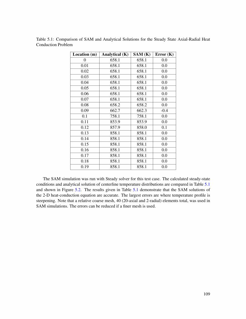
Table 5.1: Comparison of SAM and Analytical Solutions for the Steady State Axial-Radial HeatConduction Problem

Location (m) Analytical (K) SAM (K) Error (K)0 658.1 658.1 0.0

0.01 658.1 658.1 0.00.02 658.1 658.1 0.00.03 658.1 658.1 0.00.04 658.1 658.1 0.00.05 658.1 658.1 0.00.06 658.1 658.1 0.00.07 658.1 658.1 0.00.08 658.2 658.2 0.00.09 662.7 662.3 -0.40.1 758.1 758.1 0.00.11 853.9 853.9 0.00.12 857.9 858.0 0.10.13 858.1 858.1 0.00.14 858.1 858.1 0.00.15 858.1 858.1 0.00.16 858.1 858.1 0.00.17 858.1 858.1 0.00.18 858.1 858.1 0.00.19 858.1 858.1 0.0

The SAM simulation was run with Steady solver for this test case. The calculated steady-stateconditions and analytical solution of centerline temperature distributions are compared in Table 5.1and shown in Figure 5.2. The results given in Table 5.1 demonstrate that the SAM solutions ofthe 2-D heat-conduction equation are accurate. The largest errors are where temperature profile issteepening. Note that a relative coarse mesh, 40 (20-axial and 2-radial) elements total, was used inSAM simulations. The errors can be reduced if a finer mesh is used.

109

600

650

700

750

800

850

900

0 0.05 0.1 0.15 0.2

Centerlin

eTem

perature(K)

AxialPosition

Analytical

SAM

Figure 5.2: Comparisons of centerline temperature distributions of the heated rod, 2D conduction.

The input file of this example problem is shown as follows:[GlobalParams]

global_init_T = 400Tsolid_sf = 1e-1[./ PBModelParams]

p_order = 2[../]

[]

[Functions][./ T_amb_fn]

type = PiecewiseLinearx = '0 0.099 0.101 0.2'y = '300 300 500 500'axis = x

[../][]

[MaterialProperties][./fuel -mat]

type = SolidMaterialPropsk = 2Cp = 100rho = 1.0e3

[../][]

110

[Components][./ hs1]

type = PBCoupledHeatStructureposition = '0 0 0'orientation = '0 0 1'hs_type = cylinder

length = 0.2radius_i = 0.0width_of_hs = 0.005elem_number_radial = 2elem_number_axial = 20dim_hs = 2material_hs = 'fuel -mat'

heat_source_solid = 6.3661977 e7

Ts_init = 400HS_BC_type = 'Adiabatic Convective 'T_amb_right = T_amb_fnHw_right = 1e3

[../][]

[Postprocessors][./ max_T]

type = NodalMaxValueblock = 'hs1:hs'variable = T_solid

[../][]

[VectorPostprocessors][./ Tsolid]

type = NodalValueSamplerblock = 'hs1:hs'variable = T_solidsort_by = y

[../][]


[./ SMP_PJFNK]type = SMPfull = truesolve_type = 'PJFNK '

[../][] # End preconditioning block

[Executioner]type = Steady

petsc_options_iname = '-ksp_gmres_restart -pc_type 'petsc_options_value = '100 lu'

nl_rel_tol = 1e-9nl_abs_tol = 1e-6nl_max_its = 10


[./ Quadrature]type = SIMPSON

111

order = SECOND[../]

[] # close Executioner section

[Outputs]perf_graph = trueprint_linear_residuals = false[./ out_displaced]

type = Exodususe_displaced = trueexecute_on = 'initial timestep_end 'sequence = false

[../][./ csv]

type = CSV[../][./ console]

type = Console[../]

[]

112

5.2 Single Channel Flow

A simple pipe flow problem is presented here, with fixed constant or time-varying boundaryconditions. The inlet temperature of the one-meter pipe is fixed at 628 K, or oscillates following asinusoidal distribution, Tin(t) = 628+100sin(πt); the inlet velocity is fixed, uin(t)=0.5 m/s; and theinitial pipe temperate is at 628 K. After executing the test problems, the results can be imported intoParaview for visualization, as shown in Figure 5.3. The transient responses of the inlet temperaturewave propagation problem are shown in Figure 5.4, where the code predictions agreed very wellwith the analytical solutions. This is because of the high-order accuracy in both spatial and temporal(BDF2) discretizations used in SAM.

Figure 5.3: Example of SAM results shown in Paraview.

The input file of this example problem is shown as follows:

[GlobalParams]global_init_P = 1.0e5 # Global initial fluid pressureglobal_init_V = 0.5 # Global initial temperature for fluid and solidglobal_init_T = 628.15 # Global initial fluid velocityscaling_factor_var = '1 1e-3 1e-6' # Scaling factors for fluid variables (p, v, T)

[]

[EOS][./ eos] # EOS name

type = PBSodiumEquationOfState # Using the sodium equation -of-state[../]

[]

113

Figure 5.4: Transient responses of the pipe under inlet temperature oscillation, BDF2.

[Functions][./ tin_sine] # Function name

type = ParsedFunction # Parsed functionvalue = 628+100* sin(pi*t) # Parsed function formula

[../][]

[Components][./ pipe1]

type = PBOneDFluidComponenteos = eos # The equation -of-state nameposition = '0 0 0' # The origin position of this componentorientation = '0 0 1' # The orientation of the componentheat_source = 0 # Volumetric heat sourcef=0.01 # Specified friction coefficientDh = 0.02 # Equivalent hydraulic diameterlength = 1 # Length of the componentn_elems = 100 # Number of elements used in discretizationA = 3.14e-4 # Area of the One -D fluid component

[../]

[./ inlet]type = PBTDJinput = 'pipe1(in)' # Name of the connected components and the end typeeos = eos # The equation -of-statev_bc = 0.5 # Velocity boundary conditionT_bc = 628 # or T_fn = tin_sine # Temperature boundary condition

[../]

[./ outlet]

114

type = PressureOutletinput = 'pipe1(out) ' # Name of the connected components and the end typeeos = eos # The equation -of-statep_bc = '1.0e5' # Pressure boundary condition

[../][]


[./ SMP_PJFNK]type = SMP # Single -Matrix Preconditionerfull = true # Using the full set of couplings among all variablessolve_type = 'PJFNK ' # Using Preconditioned JFNK solution methodpetsc_options_iname = '-pc_type ' # PETSc option , using preconditiongpetsc_options_value = 'lu' # PETSc option , using 'LU' precondition type

# in Krylov solve[../]

[] # End preconditioning block

[Executioner]type = Transient # This is a transient simulation

dt = 0.02 # Targeted time step sizedtmin = 1e-5 # The allowed minimum time step size

petsc_options_iname = '-ksp_gmres_restart ' # Additional PETSc settings , name listpetsc_options_value = '100' # Additional PETSc settings , value list

nl_rel_tol = 1e-7 # Relative nonlinear tolerance for each Newton solvenl_abs_tol = 1e-6 # Relative nonlinear tolerance for each Newton solvenl_max_its = 20 # Number of nonlinear iterations for each Newton solve


start_time = 0.0 # Physical time at the beginning of the simulationnum_steps = 200 # Max. simulation time stepsend_time = 100. # Max. physical time at the end of the simulation

[./ Quadrature]type = TRAP # Using trapezoid integration ruleorder = FIRST # Order of the quadrature

[../][] # close Executioner section

[Outputs][./ console]

type = Console # Screen outputperf_log = true # Output the performance log


type = Exodus # Output simulation data to an ExodusII fileuse_displaced = true # Use displaced meshexecute_on = 'initial timestep_end ' # Output data at the beginning of the simulation

# and each time stepsequence = false # Don't save sequential file output per time step

[../][]

115

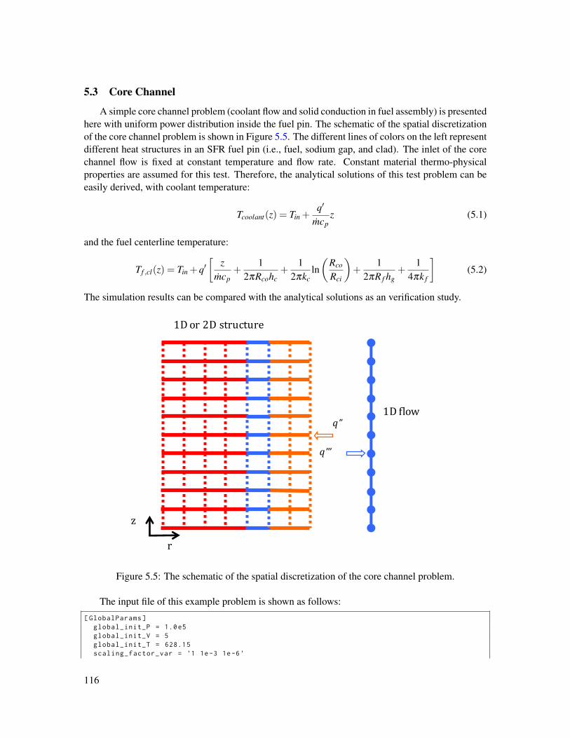
5.3 Core Channel

A simple core channel problem (coolant flow and solid conduction in fuel assembly) is presentedhere with uniform power distribution inside the fuel pin. The schematic of the spatial discretizationof the core channel problem is shown in Figure 5.5. The different lines of colors on the left representdifferent heat structures in an SFR fuel pin (i.e., fuel, sodium gap, and clad). The inlet of the corechannel flow is fixed at constant temperature and flow rate. Constant material thermo-physicalproperties are assumed for this test. Therefore, the analytical solutions of this test problem can beeasily derived, with coolant temperature:

Tcoolant(z) = Tin +q′

mcpz (5.1)

and the fuel centerline temperature:

Tf ,cl(z) = Tin +q′[

zmcp

+1

2πRcohc+

12πkc

ln(

Rco

Rci

)+

12πR f hg

+1

4πk f

](5.2)

The simulation results can be compared with the analytical solutions as an verification study.

1Dflow

1Dor2Dstructure

r

z

q’’’

q”

Figure 5.5: The schematic of the spatial discretization of the core channel problem.


[GlobalParams]global_init_P = 1.0e5global_init_V = 5global_init_T = 628.15scaling_factor_var = '1 1e-3 1e-6'

116

Tsolid_sf = 1e-3 # Scaling factors for solid temperature[]

[EOS][./ eos] # EOS name

type = PTConstantEOSp_0 = 1e5 # Pa, reference pressurerho_0 = 865.51 # kg/mˆ3, reference densitybeta = 2.7524e-4 # Kˆ{-1}, thermal expansion coefficientcp = 1272.0 # specific heat;h_0 = 7.9898 e5 # J/kg, enthalpy at reference temperatureT_0 = 628.15 # K, reference temperaturemu = 2.6216e-4 # Pa-s, dynamic viscosityk = 72 # W/K/m, thermal conductivity

[../][]

[Materials][./fuel -mat] # Material name

type = SolidMaterialPropsk = 16 # Thermal conductivityCp = 191.67 # Specific heatrho = 1.4583 e4 # Density

[../][./gap -mat] # Material name

type = SolidMaterialPropsk = 64 # Thermal conductivityCp = 1272 # Specific heatrho = 865 # Density

[../][./clad -mat] # Material name

type = SolidMaterialPropsk = 26 # Thermal conductivityCp = 638 # Specific heatrho = 7.646e3 # Density

[../][./duct -mat] # Material name

type = SolidMaterialPropsk = 26 # Thermal conductivityCp = 638 # Specific heatrho = 6e3 # Density

[../][]

[Functions]active = 'uniform '[./ uniform] # Function name

type = PiecewiseLinear # Function typeaxis = 0 # X-co-ordinate is used for xx = '0 0.8' # The x abscissa valuesy = '1 1' # The y abscissa values

[../][]

[Components][./ reactor]

type = ReactorPowerinitial_power = 3e4 # Initial total reactor power

[../][./ CH1] # Component name

type = PBCoreChannel # PBCorechannel componenteos = eos # The equation -of-state nameposition = '0 0 0'orientation = '0 0 1'

117

A = 2e-05Dh = 3.1830989e-3length = 0.8n_elems = 16

f = 0.017 # User specified friction coefficientHw = 1.6e5 # User specified heat transfer coefficientHT_surface_area_density = 1256.637 # Heat transfer surface area density , Ph/Ac

name_of_hs = 'fuel gap clad' # Heat structure namesTs_init = 628.15 # Initial structure temperaturen_heatstruct = 3 # Number of heat structuresfuel_type = cylinder # Fuel geometric type , cylinder or platewidth_of_hs = '0.003015 0.000465 0.00052 ' # The width of all heat structureselem_number_of_hs = '20 2 2' # The element numbers of all heat structuresmaterial_hs = 'fuel -mat gap -mat clad -mat' # The material used for all heat structurespower_fraction = '1.0 0.0 0.0' # The power fractions of all heat structurespower_shape_function = uniform # the axial power shape function name

[../]

#Boundary components[./ inlet]

type = PBTDJinput = 'CH1(in)'v_bc = 8.6654T_bc = 628.15eos = eos

[../][./ outlet]

type = PBTDVinput = 'CH1(out)'p_bc = '2.0e5'T_bc = 728.15eos = eos

[../][]

[Postprocessors][./ max_Tcoolant] # Output maximum fluid temperature of block CH1:pipe

type = NodalMaxValueblock = 'CH1:pipe'variable = temperature

[../][./ max_Tw] # Output maximum wall temperature of block CH1:pipe

type = NodalMaxValueblock = 'CH1:pipe'variable = Tw

[../][./ max_Tclad] # Output maximum solid temperature of block CH1:solid:clad

type = NodalMaxValueblock = 'CH1:solid:clad'variable = T_solid

[../][./ max_Tf] # Output maximum solid temperature of block CH1: solid:fuel

type = NodalMaxValueblock = 'CH1:solid:fuel'variable = T_solid

[../][]


118

[./ SMP_PJFNK]type = SMPfull = truesolve_type = 'PJFNK 'petsc_options_iname = '-pc_type 'petsc_options_value = 'lu'

[../]



petsc_options_iname = '-ksp_gmres_restart 'petsc_options_value = '300'


l_tol = 1e-5l_max_its = 50

[./ Quadrature]type = TRAPorder = FIRST


[Outputs][./ out]

type = Checkpoint # Save snapshots of the simulation data[../][./ console]

type = Consoleperf_log = true



[../][]

119

5.4 Heat Exchanger

An example of a counter-current heat exchanger problem is presented here. The inlet tempera-tures are 783 K and 606 K for the primary and secondary pipes. The mass flow rates are also fixed atthe inlets of the two sides. Because the flow rates are very close for the two sides, linear temperaturedistributions are expected for the two sides, as the code predictions shown in Figure 5.6.

600620640660680700720740760780800

0 1 2 3

Tem

pera

ture

(K

)

Axial Position (m)

primarysecondary

Figure 5.6: Temperature distribution of a counter-current heat exchanger.


global_init_P = 1.0e5global_init_V = 1global_init_T = 628.15scaling_factor_var = '1 1e-3 1e-6'Tsolid_sf = 1e-3

[]

[EOS][./ eos]

type = PBSodiumEquationOfState[../]

[]

[Materials][./ss -mat]

type = SolidMaterialPropsk = 10Cp = 638rho = 6e3

[../][]

[Components][./ IHX]

120

type = PBHeatExchangereos = eos # EOS of the primary sideeos_secondary = eos # EOS of the secondary sideposition = '0 0 0'orientation = '1 0 0'A = 0.766 # Flow area of the primary sideA_secondary = 0.517 # Flow area of the secondary sideDh = 0.0186 # Hydraulic diameter of the primary sideDh_secondary = 0.014 # Hydraulic diameter of the secondary sidelength = 3.71n_elems = 20

Hw = 1.6129 e5 # User specified heat transfer coefficient# for primary pipe

Hw_secondary = 1.6129 e5 # User specified heat transfer coefficient# for secondary pipe

HTC_geometry_type = Pipe # Geometry type of the primary pipe ,# pipe or bundle

HTC_geometry_type_secondary = Pipe # Geometry type of the secondary pipeHT_surface_area_density = 729 # Heat transfer surface area of the

# primary side , Ph/AcHT_surface_area_density_secondary = 1080.1 # Heat transfer surface area of the

# secondary side , Ph/Ac

f = 0.022 # User specified friction coefficient for primary pipef_secondary = 0.022 # User specified friction coefficient for secondary pipeinitial_V_secondary = -2 # Initial velocity for secondary pipe

Twall_init = 628.15 # Initial wall temperaturewall_thickness = 0.0033 # Wall thickness

dim_wall = 1 # Dimensions of the wall , 1D or 2Dmaterial_wall = ss-mat # Wall materialn_wall_elems = 2 # The number of elements in the radial direction

[../]

[./ inlet1]type = PBTDJinput = 'IHX(primary_in)'eos = eosv_bc = 2T_bc = 783.15

[../]

[./ outlet1]type = PressureOutletinput = 'IHX(primary_out)'eos = eosp_bc = 1.0e5

[../]

[./ inlet2]type = PBTDJinput = 'IHX(secondary_in)'eos = eosv_bc = -2T_bc = 606.15

[../]

[./ outlet2]type = PressureOutletinput = 'IHX(secondary_out)'eos = eosp_bc = 1.0e5

121

[../][]



[../]


[Postprocessors]# The total heat removal rate at the primary side of IHX[./ heat_removal_primary]

type = HeatExchangerHeatRemovalRateblock = IHX:primary_pipeheated_perimeter = 558.414

[../]# The total heat removal rate at the secondary side of IHX[./ heat_removal_secondary]

type = HeatExchangerHeatRemovalRateblock = IHX:secondary_pipeheated_perimeter = 558.414

[../][]

[Executioner]type = Transient # try Steady solver as well

dt = 0.2dtmin = 1e-4




start_time = 0.0num_steps = 10end_time = 100.



[Outputs][./ out_displaced]


[../]

122

[./ console]type = Consoleperf_log = true

[../][]

123

5.5 Volume Branch

An example problem with a VolumeBranch component included is presented here. The bound-ary and the initial conditions of the five pipes are shown in Figure 5.7 and Figure 5.8. Note thatvery different inlet orifice coefficients have been used for the connecting nodes. The volume of thePBVolumeBranch is 0.0314 m3, and the initial temperature of the volume is at 628.15 K. BecausePipe 3 has very high inlet flow rate but low inlet temperature, the temperature at the VolumeBranch,outlet of Pipes 4 and 5 will decrease correspondingly, as shown in Figure 5.9.

PBVolumeBranchPout

Pout

Vin,Tin

Vin,Tin

Vin,Tin Pipe3

Pipe2

Pipe1

Pipe4

Pipe5

Figure 5.7: The three-pipe-in and two-pipe-out VolumeBranch test model.

124

Component Pipe 1 Pipe 2 Pipe 3 Pipe 4 Pipe 5

Length (m) 1 1 1 1 1

Diameter (m) 0.02 0.02 0.02 0.02 0.02

Boundary Type Flow inlet Flow inlet Flow inlet Pressure

outlet Pressure outlet

Orifice Coeff. to

VolumeBranch 0.01 0.01 0.01 0.01 100

Z-coordinate of the node

connected to

VolumeBranch (m)

0 0.25 0.75 1 0.5

Boundary Conditions

Vin =1 m/s

Tin =

628.15K

Vin =1 m/s

Tin =

628.15K

Vin =10 m/s

Tin =

528.15K

Pout = 105 Pa

Tout =

628.15K

Pout = 1.5 ×105

Pa

Tout = 628.15K

Initial Conditions

Pressure (Pa) 1.5×105

Velocity (m/s) 1

Temperature (K) 628.15

Figure 5.8: Input parameters of the three pipe in and two pipe out VolumeBranch test model.

610

612

614

616

618

620

622

624

626

628

630

0 0.5 1 1.5 2

Temperature(K

)

Time(s)

VolumeBranch

Pipe4Outlet

Pipe5Outlet

Figure 5.9: Transient temperature response at the VolumeBranch and pipe outlets.


125

global_init_P = 1.2e5global_init_V = 1global_init_T = 628.15scaling_factor_var = '1 1e-3 1e-6'

[]

[EOS]active = 'eos'[./ eos]


[]


type = PBOneDFluidComponenteos = eosposition = '0 0 0'orientation = '0 0 1'

A = 3.14e-4Dh = 0.02length = 1n_elems = 10f = 0.01Hw = 0

[../]

[./ pipe2]type = PBOneDFluidComponenteos = eosposition = ' -1.5 0 1.25'orientation = '1 0 0'


[../]

[./ pipe3]type = PBOneDFluidComponenteos = eosposition = ' -1.5 0 1.75'orientation = '1 0 0'initial_T = 528.15


[../]

[./ pipe4]type = PBOneDFluidComponenteos = eosposition = '0 0 2'orientation = '0 0 1'

A = 3.14e-4

126

Dh = 0.02length = 1n_elems = 10f = 0.01Hw = 0

[../]

[./ pipe5]type = PBOneDFluidComponenteos = eosposition = '0.5 0 1.5'orientation = '1 0 0'


[../]

[./ branch1]type = PBVolumeBrancheos = eoscenter = '0 0 1.5' # The center or reference position of the volume branch

inputs = 'pipe1(out) pipe2(out) pipe3(out)'# The input connections of the volume branchoutputs = 'pipe4(in) pipe5(in)' # The output connections of the volume branchK = '0.01 0.01 0.01 0.01 100' # The form loss coefficient at all connections

Area = 3.14e-2 # Reference flow areavolume = 3.14e-2 # Total volumeinitial_T = 628.15 # Initial volume temperature

[../]

[./ inlet1]type = PBTDJinput = 'pipe1(in)'eos = eosv_bc = 1.0T_bc = 628.15

[../][./ inlet2]

type = PBTDJinput = 'pipe2(in)'eos = eosv_bc = 1.0T_bc = 628.15

[../][./ inlet3]

type = PBTDJinput = 'pipe3(in)'eos = eosv_bc = 10.0T_bc = 528.15

[../][./ outlet1]

type = PBTDVinput = 'pipe4(out)'eos = eosp_bc = '1.0e5'T_bc = 628.15

[../][./ outlet2]

127

type = PBTDVinput = 'pipe5(out)'eos = eosp_bc = '1.5e5'T_bc = 628.15

[../][]

[Preconditioning][./ SMP_PJFNK]

type = SMPfull = truesolve_type = 'PJFNK 'petsc_options_iname = '-pc_type 'petsc_options_value = 'lu'


[Executioner]type = Transient

dt = 1e-1dtmin = 1e-5

# setting time step range# Time step size is controlled by this TimeStepper[./ TimeStepper]

type = FunctionDTtime_t = ' 0 0.1 0.2 20 21 100 101 1e5' # Physical timetime_dt ='0.01 0.01 0.1 0.1 0.5 0.5 1 1' # Time step size dependent on

# the physical time[../]




start_time = 0.0num_steps = 100end_time = 2.



[Outputs][./ out_displaced]


[../]


128

[../][]

129

5.6 A Simple Loop Model

An example problem with a simple loop problem is presented here. It consists of six 1-Dpipes (PBOneDFluidComponent) and a heat exchanger (PBHeatExchanger). One pipe is internallyheated, as shown in Figure 5.10. The primary loop (including the heat exchanger) is connected by aset of PBSingleJunctions, a PBBranch, and a Pump. The secondary side of the heat exchanger hasfixed inlet velocity and temperature and fixed outlet pressure boundary conditions. Note that if thePump is replaced by a PBBranch, the loop will be derived by natural circulation.

TDV

TDJ

TDV

Pump%

Heated%

HX%

Figure 5.10: Schematics of the a test loop problem.


global_init_P = 1.1e5global_init_V = 0.1global_init_T = 628.15Tsolid_sf = 1e-1

[./ PBModelParams]pbm_scaling_factors = '1 1e-3 1e-6'

[../][]

[EOS][./ eos]


[]

[Materials][./ss -mat]

130

type = SolidMaterialPropsk = 20Cp = 638rho = 6e3

[../][]


type = PBOneDFluidComponenteos = eosposition = '0 1 0'orientation = '0 -1 0'

A = 0.44934Dh = 2.972e-3length = 1n_elems = 10f = 0.001

[../]

[./ CH1]type = PBOneDFluidComponenteos = eosposition = '0 0 0'orientation = '0 0 1'

A = 0.44934Dh = 2.972e-3length = 0.8n_elems = 10

f = 0.022 #McAdamsheat_source = 5e7

[../]

[./ pipe2]type = PBOneDFluidComponenteos = eosposition = '0 0 0.8'orientation = '0 0 1'

A = 0.44934Dh = 2.972e-3length = 5.18n_elems = 10f = 0.001

[../]

[./ pipe3]type = PBOneDFluidComponenteos = eosposition = '0 0 5.98'orientation = '0 1 0'

A = 0.44934Dh = 2.972e-3length = 1n_elems = 10f = 0.001

[../]

[./ IHX]type = PBHeatExchanger

131

eos = eoseos_secondary = eos

position = '0 0.976 5.98'orientation = '0 0 -1'A = 0.44934Dh = 0.0186A_secondary = 0.44934Dh_secondary = 0.0186length = 0.8n_elems = 20f = 0.022

initial_V_secondary = -0.2

HT_surface_area_density = 1e3HT_surface_area_density_secondary = 1e3

Twall_init = 628.15wall_thickness = 0.004

dim_wall = 1material_wall = ss-matn_wall_elems = 2

[../]

[./ pipe4]type = PBOneDFluidComponenteos = eosposition = '0 1.0 5.18'orientation = '0 0 -1'

A = 0.44934Dh = 2.972e-3length = 5.18n_elems = 10f = 0.001

[../]

[./ Branch1]type = PBSingleJunctioninputs = 'pipe1(out)'outputs = 'CH1(in) 'eos = eos

[../][./ Branch2]

type = PBSingleJunctioninputs = 'CH1(out) 'outputs = 'pipe2(in)'eos = eos

[../][./ Branch3]

type = PBBranchinputs = 'pipe2(out)'outputs = 'pipe3(in) pipe5(in)'K = '0.0 0.0 10.0'Area = 0.44934initial_P = 1e5eos = eos

[../][./ Branch4]

type = PBSingleJunctioninputs = 'pipe3(out)'outputs = 'IHX(primary_in)'

132

eos = eos[../][./ Branch5]

type = PBSingleJunctioninputs = 'IHX(primary_out)'outputs = 'pipe4(in)'eos = eos

[../]

###### switch between Brach6 and Pump_p for natural circulation or forced flow

# [./ Pump_p]# type = PBPump # This is a PBPump component# eos = eos# inputs = 'pipe4(out)'# outputs = 'pipe1(in)'# K = '1. 1.' # Form loss coefficient at pump inlet and outlet# Area = 0.44934 # Reference pump flow area# initial_P = 1.5e5 # Initial pressure# Head = 5e3 # Pump head , Pa# [../]

[./ Branch6]type = PBSingleJunctioninputs = 'pipe4(out)'outputs = 'pipe1(in)'eos = eos

[../]

[./ pipe5]type = PBOneDFluidComponenteos = eosposition = '0 0 5.98'orientation = '0 0 1'A = 0.44934Dh = 2.972e-3length = 0.1n_elems = 2f = 0.001

[../][./ p_out]

type = PressureOutletinput = 'pipe5(out)'eos = eosp_bc = '1e5'

[../]

[./ inlet2]type = PBTDJinput = 'IHX(secondary_in)'eos = eosv_bc = -1T_bc = 606.15

[../]

[./ outlet2]type = PressureOutletinput = 'IHX(secondary_out)'eos = eosp_bc = 1.0e5

[../][]

[Postprocessors]

133

# Output mass flow rate at inlet of CH1[./ CH1_flow]

type = ComponentBoundaryFlowinput = CH1(in)

[../][]

[Preconditioning]active = 'SMP_PJFNK '[./ SMP_PJFNK]

type = SMPfull = truesolve_type = 'PJFNK 'petsc_options_iname = '-pc_type -ksp_gmres_restart 'petsc_options_value = 'lu 101'

[../][]


nl_rel_tol = 1e-8nl_abs_tol = 1e-7nl_max_its = 20l_tol = 1e-6l_max_its = 100


[../][]

[Outputs]print_linear_residuals = false[./ out_displaced]


[../]


[../][]

134

5.7 A Simplified SFR Model

A typical pool-type SFR test problem is presented here, based on the design information of theAdvanced Burner Test Reactor (ABTR) conceptual design [17]. Figure 5.11 shows the schematicsof the test SFR model. The primary coolant system consists of the downcomers (pump outlet andpump discharge), the lower plenum, the reactor core model, the upper plenum, and the intermediateheat exchanger. Five PBCoreChannels are used to describe the reactor core. PBLiquidVolume com-ponents are used to represent the cold pool and the upper plenum. Both are connected to a CoverGascomponent. Different components are connected with junction Components. The intermediate loop,the secondary loop, and the DRACS loop are modeled with great simplicities. Single-phase countercurrent heat exchanger models (PBHeatExchanger) are used to mimic the function of the intermedi-ate loop heat exchanger (IHX), DRACS heat exchanger (DHX), and secondary loop heat exchanger(SHX) to transfer heat among the primary, intermediate, secondary, and the DRACS loops.

TDV$

TDJ$

DHX$

Cold$Pool$Inlet$Plenum$

Outlet$Plenum$(Hot$Pool)$

TDV$

TDJ$

Pump$

IHX$ Na9CO2$HX$

Core$Channels$

TDV$

Figure 5.11: Schematics of the a simple pool-type SFR model.


[GlobalParams]global_init_P = 2e5global_init_V = 0.1global_init_T = 628.15Tsolid_sf = 1e-3

[./ PBModelParams]pbm_scaling_factors = '1 1e-3 1e-6'

135

pspg = falsep_order = 2

[../][]

[EOS][./ eos]


[]

[Functions][./ ppf_axial]

type = PiecewiseLinearx = '0.0 0.0200 0.0600 0.100 0.140 0.180 0.220 0.260 0.300 0.340 0.380

0.420 0.460 0.500 0.540 0.580 0.620 0.660 0.700 0.740 0.780 0.800'y = '7.818e-1 8.12035e-1 8.72501e-1 9.43054e-1 1.01107 1.04739 1.09779 1.137901.16662 1.17569 1.18022

1.17255 1.15267 1.13305 1.08829 1.03142 9.62681e-1 9.08601e-1 8.11380e-17.04156e-1 5.90929e-1 5.34316e-1'

axis = 0[../]

[./ power_history]type = PiecewiseLinear

x =' -1.000E+03 5.000E-01 1.000E+00 1.500E+00 2.000E+00 2.500E+00 3.000E+003.500E+00 4.000E+00 4.500E+00

5.000E+00 5.500E+00 6.000E+00 6.500E+00 7.000E+00 7.500E+00 8.000E+00 8.500E+009.000E+00 9.500E+00

1.000E+01 1.050E+01 1.100E+01 1.150E+01 1.200E+01 1.250E+01 1.300E+01 1.350E+011.400E+01 1.450E+01

1.500E+01 1.550E+01 1.600E+01 1.650E+01 1.700E+01 1.750E+01 1.800E+01 1.850E+011.900E+01 1.950E+01

2.000E+01 2.500E+01 3.000E+01 3.500E+01 4.000E+01 4.500E+01 5.000E+01 5.500E+016.000E+01 6.500E+01

7.000E+01 7.500E+01 8.000E+01 8.500E+01 9.000E+01 9.500E+01 1.000E+02 1.100E+021.200E+02 1.300E+02

1.400E+02 1.500E+02 1.600E+02 1.700E+02 1.800E+02 1.900E+02 2.000E+02 2.100E+022.200E+02 2.300E+02

2.400E+02 2.500E+02 2.600E+02 2.700E+02 2.800E+02 2.900E+02 3.000E+02 3.200E+023.400E+02 3.600E+02

3.800E+02 4.000E+02 4.500E+02 5.000E+02 5.500E+02 6.000E+02 6.500E+02 7.500E+021.000E+03 2.000E+03

4.000E+03 6.000E+03 8.000E+03 1.000E+04 1.500E+04 2.000E+04 2.500E+04 3.000E+043.500E+04 4.000E+04 1e5'

y ='1.000E+00 1.000E+00 9.969E-01 9.892E-01 9.784E-01 1.537E-01 1.390E-011.292E-01 1.215E-01 1.152E-01

1.097E-01 1.050E-01 1.008E-01 9.710E-02 9.377E-02 9.077E-02 8.807E-02 8.561E-028.337E-02 8.132E-02

7.944E-02 7.771E-02 7.611E-02 7.463E-02 7.325E-02 7.197E-02 7.077E-02 6.964E-026.858E-02 6.758E-02

6.663E-02 6.574E-02 6.489E-02 6.408E-02 6.331E-02 6.258E-02 6.187E-02 6.120E-026.055E-02 5.993E-02

5.933E-02 5.431E-02 5.049E-02 4.741E-02 4.485E-02 4.267E-02 4.078E-02 3.914E-023.769E-02 3.640E-02

3.526E-02 3.425E-02 3.334E-02 3.252E-02 3.178E-02 3.111E-02 3.051E-02 2.946E-022.858E-02 2.784E-02

2.720E-02 2.665E-02 2.617E-02 2.575E-02 2.537E-02 2.502E-02 2.471E-02 2.443E-022.417E-02 2.393E-02

2.370E-02 2.349E-02 2.329E-02 2.310E-02 2.292E-02 2.276E-02 2.259E-02 2.229E-022.201E-02 2.175E-02

2.151E-02 2.128E-02 2.076E-02 2.029E-02 1.987E-02 1.948E-02 1.912E-02 1.847E-021.715E-02 1.395E-02

136

1.112E-02 9.789E-03 8.994E-03 8.448E-03 7.579E-03 7.040E-03 6.657E-03 6.359E-036.117E-03 5.911E-03 4e-3'

[../]

[./ pump_p_coastdown]type = PiecewiseLinear

x =' -1.000E+03 0.00E+00 4.00E-01 8.00E-01 1.20E+00 1.60E+00 2.00E+00 2.40E+002.80E+00 3.20E+00 3.60E+00

4.00E+00 4.40E+00 4.80E+00 5.20E+00 5.60E+00 6.00E+00 6.40E+00 6.80E+007.20E+00 7.60E+00

8.000E+00 1.000E+01 2.000E+01 3.000E+01 4.000E+01 5.000E+01 6.000E+01 7.000E+018.000E+01 9.000E+01

1.000E+02 1.100E+02 1.200E+02 1.300E+02 1.400E+02 1.500E+02 1.600E+02 1.700E+021.800E+02 1.900E+02

2.000E+02 2.100E+02 2.200E+02 2.300E+02 2.400E+02 2.500E+02 2.600E+02 2.700E+022.800E+02 2.900E+02

3.000E+02 3.100E+02 3.200E+02 3.300E+02 3.400E+02 3.500E+02 3.600E+02 3.700E+023.800E+02 3.900E+02

4.000E+02 4.100E+02 4.200E+02 1.00E+05'

y ='1.000E+00 1.000E+00 9.671E-01 9.355E-01 9.050E-01 8.757E-01 8.476E-018.205E-01 7.945E-01 7.695E-01 7.455E-01

7.225E-01 7.004E-01 6.792E-01 6.590E-01 6.395E-01 6.209E-01 6.031E-01 5.860E-015.697E-01 5.540E-01

5.396E-01 4.749E-01 2.753E-01 1.773E-01 1.219E-01 8.812E-02 6.655E-02 5.206E-024.181E-02 3.425E-02

2.850E-02 2.401E-02 2.043E-02 1.754E-02 1.516E-02 1.317E-02 1.151E-02 1.009E-028.869E-03 7.816E-03

6.898E-03 6.094E-03 5.382E-03 4.752E-03 4.192E-03 3.692E-03 3.253E-03 2.814E-032.480E-03 2.132E-03

1.866E-03 1.621E-03 1.397E-03 1.190E-03 9.999E-04 8.248E-04 6.642E-04 5.175E-043.841E-04 2.637E-04

1.558E-04 5.989E-05 0 0'

scale_factor = 415100[../]

[./ pump_s_coastdown]type = PiecewiseLinear

x =' -1.000E+03 0.00E+00 4.00E-01 8.00E-01 1.20E+00 1.60E+00 2.00E+00 2.40E+002.80E+00 3.20E+00 3.60E+00

4.00E+00 4.40E+00 4.80E+00 5.20E+00 5.60E+00 6.00E+00 6.40E+00 6.80E+007.20E+00 7.60E+00

8.000E+00 1.000E+01 2.000E+01 3.000E+01 4.000E+01 5.000E+01 6.000E+01 7.000E+018.000E+01 9.000E+01

1.000E+02 1.100E+02 1.200E+02 1.300E+02 1.400E+02 1.500E+02 1.600E+02 1.700E+021.800E+02 1.900E+02

2.000E+02 2.100E+02 2.200E+02 2.300E+02 2.400E+02 2.500E+02 2.600E+02 2.700E+022.800E+02 2.900E+02

3.000E+02 3.100E+02 3.200E+02 3.300E+02 3.400E+02 3.500E+02 3.600E+02 3.700E+023.800E+02 3.900E+02

4.000E+02 4.100E+02 4.200E+02 1.00E+05'

y ='1.000E+00 1.000E+00 9.671E-01 9.355E-01 9.050E-01 8.757E-01 8.476E-018.205E-01 7.945E-01 7.695E-01 7.455E-01

7.225E-01 7.004E-01 6.792E-01 6.590E-01 6.395E-01 6.209E-01 6.031E-01 5.860E-015.697E-01 5.540E-01

5.396E-01 4.749E-01 2.753E-01 1.773E-01 1.219E-01 8.812E-02 6.655E-02 5.206E-024.181E-02 3.425E-02

2.850E-02 2.401E-02 2.043E-02 1.754E-02 1.516E-02 1.317E-02 1.151E-02 1.009E-028.869E-03 7.816E-03

6.898E-03 6.094E-03 5.382E-03 4.752E-03 4.192E-03 3.692E-03 3.253E-03 2.814E-032.480E-03 2.132E-03

1.866E-03 1.621E-03 1.397E-03 1.190E-03 9.999E-04 8.248E-04 6.642E-04 5.175E-04

137

3.841E-04 2.637E-041.558E-04 5.989E-05 0 0'

scale_factor = 40300[../]

[./ flow_secondary]type = PiecewiseLinearx =' -1.000E+03 0 1 1e5'y = ' -1259 -1259 0 0'scale_factor = 0.002216 # 1/rhoA

[../]

[./ flow_dhx]type = PiecewiseLinearx =' -1.000E+03 0 1 1e5'y = '0 0 -6.478 -6.478'scale_factor = 0.046 # 1/rhoA

[../][]

[Materials][./fuel -mat]

type = HeatConductionMaterialPropsk = 29.3Cp = 191.67rho = 1.4583 e4

[../][./gap -mat]

type = HeatConductionMaterialPropsk = 64Cp = 1272rho = 865

[../][./clad -mat]

type = HeatConductionMaterialPropsk = 26.3Cp = 638rho = 7.646e3

[../][./ss -mat]

type = HeatConductionMaterialPropsk = 26.3Cp = 638rho = 7.646e3

[../][]

[Components][./ reactor]

type = ReactorPowerinitial_power = 250e6decay_heat = power_history

[../]

###### Primary Loop ######

[./ CH1]type = PBCoreChanneleos = eosposition = '0 -1 0'orientation = '0 0 1'

A = 4.9237e-3

138

Dh = 2.972e-3length = 0.8n_elems = 4

lam_factor = 1.406turb_factor = 1.12933HTC_geometry_type = Pipe # pipe modelHT_surface_area_density = 1107.8

dim_hs = 1name_of_hs = 'fuel gap clad'Ts_init = 628.15n_heatstruct = 3fuel_type = cylinderwidth_of_hs = '0.003015 0.000465 0.00052 'elem_number_of_hs = '2 1 1'material_hs = 'fuel -mat gap -mat clad -mat'

power_fraction = '0.02248 0.0 0.0'power_shape_function = ppf_axial

[../]

[./ CH1_LP]type = PBPipeeos = eosposition = '0 -1 -0.6'orientation = '0 0 1'

A = 4.9237e-3Dh = 2.972e-3length = 0.6n_elems = 2radius_i = 0.02

lam_factor = 1.406turb_factor = 1.12933HTC_geometry_type = Pipe # pipe model

dim_wall = 1Twall_init = 628.15wall_thickness = 0.0005 #0.002n_wall_elems = 1HT_surface_area_density_wall = 1107.8material_wall = ss-matHS_BC_type = Adiabatic

[../]

[./ CH1_UP]type = PBPipeeos = eosposition = '0 -1 0.8'orientation = '0 0 1'

A = 4.9237e-3Dh = 2.972e-3length = 1.5n_elems = 2radius_i = 0.02


dim_wall = 1

139

Twall_init = 628.15wall_thickness = 0.0005n_wall_elems = 1HT_surface_area_density_wall = 1107.8material_wall = ss-matHS_BC_type = Adiabatic

[../][./ Branch_CH1_L]

type = PBSingleJunctioninputs = 'CH1_LP(out)'outputs = 'CH1(in)'eos = eos

[../][./ Branch_CH1_U]

type = PBSingleJunctioninputs = 'CH1(out)'outputs = 'CH1_UP(in)'eos = eos

[../]

[./ CH2]type = PBCoreChanneleos = eosposition = '0 -0.5 0'orientation = '0 0 1'





[../][./ CH2_LP]

type = PBPipeeos = eosposition = '0 -0.5 -0.6'orientation = '0 0 1'

A = 0.11323Dh = 2.972e-3length = 0.6n_elems = 2radius_i = 0.02


140

dim_wall = 1Twall_init = 628.15wall_thickness = 0.0005n_wall_elems = 1HT_surface_area_density_wall = 1107.8material_wall = ss-matHS_BC_type = Adiabatic

[../][./ CH2_UP]

type = PBPipeeos = eosposition = '0 -0.5 0.8'orientation = '0 0 1'








[../]

[./ CH3]type = PBCoreChanneleos = eosposition = '0 0 0'orientation = '0 0 1'



dim_hs = 1name_of_hs = 'fuel gap clad'Ts_init = 628.15

141

n_heatstruct = 3fuel_type = cylinderwidth_of_hs = '0.003015 0.000465 0.00052 'elem_number_of_hs = '2 1 1'material_hs = 'fuel -mat gap -mat clad -mat'


[../][./ CH3_LP]

type = PBPipeeos = eosposition = '0 0 -0.6'orientation = '0 0 1'




[../][./ CH3_UP]

type = PBPipeeos = eosposition = '0 0 0.8'orientation = '0 0 1'







142


[../]

[./ CH4]type = PBCoreChanneleos = eosposition = '0 0.5 0'orientation = '0 0 1'





[../][./ CH4_LP]

type = PBPipeeos = eosposition = '0 0.5 -0.6'orientation = '0 0 1'




[../][./ CH4_UP]

type = PBPipeeos = eosposition = '0 0.5 0.8'orientation = '0 0 1'

143








[../]

[./ CH5]type = PBCoreChanneleos = eosposition = '0 1 0'orientation = '0 0 1'


HTC_geometry_type = Pipe # pipe modelHT_surface_area_density = 2113.6

dim_hs = 1name_of_hs = 'fuel clad'Ts_init = 628.15n_heatstruct = 2fuel_type = cylinderwidth_of_hs = '6.32340e-3 7.0260e-4'elem_number_of_hs = '2 1'material_hs = 'fuel -mat clad -mat'

power_fraction = '0.02860 0.0'power_shape_function = ppf_axial

[../][./ CH5_LP]

type = PBPipeeos = eosposition = '0 1 -0.6'orientation = '0 0 1'

144


HTC_geometry_type = Pipe # pipe modelHT_surface_area_density_wall = 2113.6

dim_wall = 1Twall_init = 628.15wall_thickness = 0.001 #0.0035n_wall_elems = 1material_wall = ss-matHS_BC_type = Adiabatic

[../][./ CH5_UP]

type = PBPipeeos = eosposition = '0 1 0.8'orientation = '0 0 1'

A = 0.153955129Dh = 1.694e-3

length = 1.5n_elems = 2radius_i = 0.02

HTC_geometry_type = Pipe # pipe modelHT_surface_area_density_wall = 2113.6

dim_wall = 1Twall_init = 628.15wall_thickness = 0.001 #0.0035n_wall_elems = 1material_wall = ss-matHS_BC_type = Adiabatic





[../]

[./ IHX]type = PBHeatExchangereos = eoseos_secondary = eosposition = '0 1.5 5.88'orientation = '0 0 -1'A = 0.766A_secondary = 0.517Dh = 0.0186Dh_secondary = 0.014length = 3.71

145

n_elems = 4initial_V_secondary = -2

HTC_geometry_type = Pipe # pipe modelHTC_geometry_type_secondary = PipeHT_surface_area_density = 729HT_surface_area_density_secondary = 1080.1

Twall_init = 628.15wall_thickness = 0.0033


[../]

[./ pump_pipe]type = PBOneDFluidComponenteos = eosposition = '0 -1.5 3.61'orientation = '0 0 -1'

A = 0.132Dh = 0.34length = 4.38n_elems = 4f = 0.001Hw = 0

[../]

[./ pump_discharge]type = PBOneDFluidComponenteos = eosposition = '0 -1.5 -0.77'orientation = '0 1 0'

A = 5.36Dh = 1length = 1.26n_elems = 2f = 0.001Hw = 0

[../]

[./ inlet_plenum]type = PBVolumeBranchcenter = '0 0 -0.77'inputs = 'pump_discharge(out)'outputs = 'CH1_LP(in) CH2_LP(in) CH3_LP(in) CH4_LP(in) CH5_LP(in)'K = '0.2 0.5 5.2 6.0 13.8 12480'Area = 0.44934volume = 3.06

initial_P = 3e5initial_T = 628.15eos = eosdisplay_pps = truenodal_Tbc = true

[../]

[./ hot_pool]type = PBLiquidVolumecenter = '0 0 6.45'

146

inputs = 'CH1_UP(out) CH2_UP(out) CH3_UP(out) CH4_UP(out) CH5_UP(out)'outputs = 'IHX(primary_in)'K = '0.5 0.5 0.5 0.5 0.5 5.0'Area = 11.16volume = 92.51

initial_level = 2.16 #3.59initial_T = 783.15initial_V = 0.00356display_pps = trueeos = eoscovergas_component = 'cover_gas '

[../]

[./ cold_pool]type = PBLiquidVolumecenter = '0 0 2.3'inputs = 'IHX(primary_out) DHX(primary_out)'outputs = 'pump_pipe(in) DHX(primary_in)'

K = '0.1 0.1 0.2 0.1 'Area = 23.96volume = 152.97

initial_level = 5initial_T = 628.15initial_P = 3e5display_pps = trueeos = eoscovergas_component = 'cover_gas '

[../][./ cover_gas]

type = CoverGasn_liquidvolume =2name_of_liquidvolume = 'hot_pool cold_pool 'initial_P = 1e5initial_Vol = 66.77initial_T = 783.15

[../][./ Pump_p]

type = PBPumpeos = eosinputs = 'pump_pipe(out)'outputs = 'pump_discharge(in)'

K = '1. 1.'Area = 0.055initial_P = 3e5

Head = 415100Head_fn = pump_p_coastdown

[../]

###### Secondary Loop ######[./ pipe8]

type = PBOneDFluidComponenteos = eosposition = '0 2.7 2.17'orientation = '0 -1 0'

A = 0.092Dh = 0.34length = 1n_elems = 2

147

f = 0.001Hw = 0

[../]

[./ pipe9]type = PBOneDFluidComponenteos = eosposition = '0 1.7 5.88'orientation = '0 1 0'

A = 0.092Dh = 0.34length = 1n_elems = 2f = 0.001Hw = 0

[../]

[./ NaHX]type = PBHeatExchangereos = eoseos_secondary = eosposition = '0 2.7 5.88'orientation = '0 0 -1'A = 0.766A_secondary = 0.517Dh = 0.0186Dh_secondary = 0.014length = 3.71n_elems = 4initial_V_secondary = -2.8

HTC_geometry_type = Pipe # pipe modelHTC_geometry_type_secondary = PipeHT_surface_area_density = 729HT_surface_area_density_secondary = 1080.1

Twall_init = 628.15wall_thickness = 0.0008 #0.00174 , 0.00087


[../]

[./ Branch8]type = PBBranchinputs = 'pipe8(out)'outputs = 'IHX(secondary_in)'K = '0.05 0.05'Area = 0.092initial_P = 2e5eos = eos

[../]

[./ Branch9]type = PBBranchinputs = 'IHX(secondary_out)'outputs = 'pipe9(in)'K = '0.0 0.0'Area = 0.092initial_P = 2e5eos = eos

[../]

148

[./ Branch10]type = PBBranchinputs = 'pipe9(out) 'outputs = 'NaHX(primary_in)'K = '0.01 0.01 'Area = 0.092initial_P = 2e5eos = eos

[../]

[./ Pump_s]type = PBPumpeos = eosinputs = 'NaHX(primary_out)'outputs = 'pipe8(in)'

K = '0.1 0.1'Area = 0.766

initial_P = 2e5

Head = 40300Head_fn = pump_s_coastdown

[../]

[./ secondary_p]type = ReferenceBoundaryinput = 'NaHX(primary_in)'variable = 'pressure 'value = 1e5

[../]

###### Power conversion loop ######

[./ NaLoop_in]type = PBTDJinput = 'NaHX(secondary_in)'v_fn = flow_secondaryT_bc = 596.75eos = eosweak_bc = true

[../]

[./ NaLoop_out]type = PressureOutletinput = 'NaHX(secondary_out)'p_bc = '1e5'eos = eos

[../]

###### DRACS loop ######[./ DHX]

type = PBHeatExchangereos = eoseos_secondary = eosposition = '0 -1.5 6.04'orientation = '0 0 -1'A = 0.024A_secondary = 0.024Dh = 0.037Dh_secondary = 0.037length = 2.35n_elems = 4

149

HTC_geometry_type = Pipe # pipe modelHTC_geometry_type_secondary = PipeHT_surface_area_density = 108.1HT_surface_area_density_secondary = 108.1

Twall_init = 628.15dim_wall = 1wall_thickness = 0.0045material_wall = ss-mat

n_wall_elems = 1[../]

[./ DRACS_inlet]type = PBTDJinput = 'DHX(secondary_in)'v_fn = flow_dhxT_bc = 450.3eos = eoswall_bc = true

[../][./ DRACS_outlet]

type = PressureOutletinput = 'DHX(secondary_out)'p_bc = 1.3e5eos = eos

[../][]

[Postprocessors][./ pump_flow]

type = ComponentBoundaryFlowinput = pump_pipe(in)

[../][./ IHX_primaryflow]

type = ComponentBoundaryFlowinput = IHX(primary_in)

[../][./ IHX_secondaryflow]

type = ComponentBoundaryFlowinput = IHX(secondary_in)

[../][./ DHX_flow]

type = ComponentBoundaryFlowinput = DHX(primary_in)

[../][./ IHX_inlet_T]

type = ComponentBoundaryVariableValueinput = IHX(primary_in)variable = temperature

[../][./ CH1_velocity]

type = ComponentBoundaryVariableValueinput = CH1(in)variable = velocity




type = ComponentBoundaryVariableValue

150

input = CH3(in)variable = velocity





[../][./ CH1_outlet_flow]

type = ComponentBoundaryFlowinput = CH1_UP(out)









[../][./ CH1_outlet_T]

type = ComponentBoundaryVariableValueinput = CH1_UP(out)variable = temperature









[../][./ max_Tcoolant_core]

type = NodalMaxValueblock = 'CH1:pipe CH2:pipe CH3:pipe CH4:pipe'variable = temperature

[../][./ max_Tco_core]

151

type = NodalMaxValueblock = 'CH1:pipe CH2:pipe CH3:pipe CH4:pipe'variable = Tw

[../][./ max_Tci_core]

type = NodalMaxValueblock = 'CH1:solid:clad CH2:solid:clad CH3:solid:clad CH4:solid:clad'variable = T_solid

[../][./ max_Tf_core]

type = NodalMaxValueblock = 'CH1:solid:fuel CH2:solid:fuel CH3:solid:fuel CH4:solid:fuel'variable = T_solid

[../][./ max_Tcoolant_Ref]

type = NodalMaxValueblock = 'CH5:pipe'variable = temperature

[../][./ max_Tco_Ref]

type = NodalMaxValueblock = 'CH5:pipe'variable = Tw

[../][./ max_Tci_Ref]

type = NodalMaxValueblock = 'CH5:solid:clad'variable = T_solid

[../][./ max_Tf_Ref]

type = NodalMaxValueblock = 'CH5:solid:fuel'variable = T_solid

[../]

[./ DHX_heatremoval]type = HeatExchangerHeatRemovalRateblock = 'DHX:primary_pipe 'heated_perimeter = 2.5944

[../][./ IHX_heatremoval]

type = HeatExchangerHeatRemovalRateblock = 'IHX:primary_pipe 'heated_perimeter = 558.414

[../][./ NaHX_heatremoval]

type = HeatExchangerHeatRemovalRateblock = 'NaHX:secondary_pipe 'heated_perimeter = 558.414

[../][]




[Executioner]

152

type = Transientdt = 0.1dtmin = 1e-3

# setting time step range[./ TimeStepper]

type = FunctionDTtime_t = ' -1000 -499.9 -499.8 -499 -498 -450 -449 -1 0 2 3

10 11 380 381 440 441 1e5'time_dt =' 0.02 0.02 0.2 0.2 0.5 0.5 2 2 0.2 0.2 0.5

0.5 2 2 2 2 2 2'min_dt = 1e-3

[../]


l_tol = 1e-4l_max_its = 100line_search = basic

start_time = -500num_steps = 10000end_time = 0

[./ Quadrature]type = SIMPSONorder = SECOND


[Outputs]print_linear_residuals = false[./ out_displaced]


[../][./ checkpoint]

type = Checkpointnum_files = 1

[../][./ console]

type = Consoleperf_log = true

[../][./ csv]

type = CSV[]

[]

153

ACKNOWLEDGMENTS

This work is funded by U.S. Department of Energy Office Nuclear Energy Advanced Modelingand Simulation (NEAMS) program.

REFERENCES

[1] R. Hu. SAM Theory Manual. Technical Report ANL/NE-17/4, Argonne National Laboratory,2017.

[2] R. Hu. Three-dimensional flow model development for thermal mixing and stratification mod-eling in reactor system transients analyses. Nuclear Engineering and Design, 345:209–215,2019.

[3] G. Hu, G. Zhang, and R. Hu. Reactivity Feedback Modeling in SAM. Technical ReportANL-NSE-19/1, Argonne National Laboratory, 2019.

[4] G. Hu, R. Hu, and L. Zou. Development of Heat Pipe Reactor Modeling in SAM. TechnicalReport ANL-NSE-19/9, Argonne National Laboratory, 2019.

[5] D. Gaston, C. Newman, G. Hansen, and D. Lebrun-Grandie. MOOSE: A parallel compu-tational framework for coupled systems of nonlinear equations. Nuclear Engineering andDesign, 239:1768–1778, 2009.

[6] B.S. Kirk, J.W. Peterson, R.H. Stogner, and F.C. Graham. libMesh: A C++ Library for ParallelAdaptive Mesh Refinement/Coarsening Simulations. Engineering with Computers, 22:237–254, 2006.

[7] PETSc. PETSc Web page., 2017. URL http://www.mcs.anl.gov/petsc.

[8] D. A. Knoll and D. E. Keyes. Jacobian-free Newton-Krylov Methods: a Survey of Approachesand Applications. Journal of Computational Physics, 193:357–397, 2004.

[9] R.A. Berry, J.W. Peterson, H. Zhang, R.C. Martineau, H. Zhao, L. Zou, D. Andrs, andJ. Hansel. RELAP-7 Theory Manual. Technical Report INL/EXT-14-31366/Revision 3, IdahoNational Laboratory, 2018.

[10] R. Hu, J.W. Thomas, E. Munkhzul, and T.H. Fanning. Coupled System and CFD Code Simu-lation of Thermal Stratification in SFR Protected Loss-Of-Flow Transients. In Proceedings ofICAPP 2014, 2014.

[11] T.H. Fanning and R. Hu. Coupling the System Analysis Module with SAS4A/SASSYS-1.Technical Report ANL/NE-16/22, Argonne National Laboratory, 2016.

[12] R. Martineau, D. Andrs, J. Hansel, C. Permann, M. Bernard, R. Johns, R. Hu, J. Wolf,H. Zhang, and R. Szilard. Extending the Capability of Nuclear Plant Systems Analysis withAdvanced Tightly-Coupled Nuclear Fuels Performance. In 2018 American Nuclear SocietyAnnual Meeting, 2018.

154

http://www.mcs.anl.gov/petsc

[13] HYPRE Web page. URL https://computation-rnd.llnl.gov/linear solvers/.

[14] MPICH2 Web page. URL http://www.mcs.anl.gov/mpich2.

[15] TBB Web page. URL https://www.threadingbuildingblocks.org/.

[16] U.S. NRC. TRACE 5.0 Assessment Manual-Appendix A: Fundamental Validation Cases.Technical report, U. S. Nuclear Regulatory Commission, 2008.

[17] Y.I. Chang, P.J. Finck, and C. Grandy. Advanced Burner Test Reactor Preconceptual De-sign Report. Technical Report ANL-ABR-1 (ANL-AFCI-173), Argonne National Laboratory,2006.

155

https://computation-rnd.llnl.gov/linear_solvers/

http://www.mcs.anl.gov/mpich2

https://www.threadingbuildingblocks.org/

Nuclear Science & Engineering DivisionArgonne National Laboratory9700 South Cass Avenue, Bldg. 208Argonne, IL 60439

www.anl.gov

Argonne National Laboratory is a U.S. Department of Energylaboratory managed by UChicago Argonne, LLC

Documents

SAM User’s Guide