samples of utility functions but never a complete analytical

Abstract of “Learning Equilibria of Simulation-Based Games: Applications to Empirical Mechanism

Design” by Enrique Areyan Viqueira, Ph.D., Brown University, May 2021.

In this thesis, we first contribute to the empirical-game theoretic analysis (EGTA) literature both

from a theoretical and a computational perspective. Theoretically, we present a mathematical frame-

work to precisely describe simulation-based games and analyze their properties. In a simulation-

based game, one only gets to observe samples of utility functions but never a complete analytical

description. We provide results that complement and strengthen previous results on guarantees of

the approximate Nash equilibria learned from samples. Computationally, we find and thoroughly

evaluate Probably Approximate Correct (PAC) learning algorithms, which we show make frugal use

of data to provably solve simulation-based games, up to a user’s given error tolerance.

Next, we turn our attention to mechanism design. When mechanism design depends on EGTA,

it is called empirical mechanism design (EMD). Equipped with our EGTA framework, we further

present contributions to EMD, in particular to parametric EMD. In parametric EMD, there is an

overall (parameterized) mechanism (e.g., a second price auction with reserve prices as parameters).

The choice of parameters then determines a mechanism (e.g., the reserve price being $10 instead of

$100). Our EMD contributions are again two-fold. From a theoretical point of view, we formulate

the problem of finding the optimal parameters of a mechanism as a black-box optimization problem.

For the special case where the parameter space is finite, we present an algorithm that, with high

probability, provably finds an approximate global optimal. For more general cases, we present a

Bayesian optimization algorithm and empirically show its e�ectiveness.

EMD is only as e�ective as the set of heuristic strategies used to optimize a mechanism’s parame-

ters. To demonstrate our methodology’s e�ectiveness, we developed rich bidding heuristics in one

specific domain: electronic advertisement auctions. These auctions are an instance of combinatorial

auctions, a vastly important auction format used in practice to allocate many goods of interest (e.g.,

electromagnetic spectra). Our work on designing heuristics for electronic advertisement led us to

contribute heuristics for the computation of approximate competitive (or Walrasian) equilibrium,

work of interest in its own right.

Learning Equilibria of Simulation-Based Games: Applications to Empirical Mechanism Design

by

Enrique Areyan Viqueira

Sc. M., Brown University, 2017

MAT., Indiana University, 2015

Sc. M., Indiana University, 2013

Licenciado en Computación, Universidad Central de Venezuela, 2010

A dissertation submitted in partial fulfillment of the

requirements for the Degree of Doctor of Philosophy

in the Department of Computer Science at Brown University

Providence, Rhode Island

May 2021

© Copyright 2021 by Enrique Areyan Viqueira

This dissertation by Enrique Areyan Viqueira is accepted in its present form by

the Department of Computer Science as satisfying the dissertation requirement

for the degree of Doctor of Philosophy.

DateAmy Greenwald, Director

Recommended to the Graduate Council

DateGeorge Konidaris, Reader

DateBenjamin Lubin, Reader

DateSerdar Kadioglu, Reader

Approved by the Graduate Council

DateAndrew G. Campbell

Dean of the Graduate School

iii

��

3/16/2021

3/15/2021

��

��

Vita

In his home country, Venezuela, Enrique Areyan Viqueira attended Universidad Central de Venezuela,

where he received a Licenciado en Computación (Sc.B. in Computer Science). He then moved to

the United States and attended graduate school at Indiana University, where he received a Master

of Science in Computer Science and a Master of Arts for Teachers with a major in Mathematics. He

then attended Brown University, receiving a Masters in Computer Science en route to his Ph.D.

At Brown, Enrique was the sole instructor for CS3: Introduction to Computation for the Hu-

manities and Social Sciences and co-instructor for CS1410: Introduction to Artificial Intelligence.

He also actively developed content for CS1951k: Algorithmic Game Theory, including hands-on lab-

oratories where students developed automated trading agents for advertisement exchange models.

He received the Paris Kanellakis fellowship for the academic year 2018-2019. In 2017, 2018, and

2019, Enrique was a summer research scientist intern for Amazon.

Together with his advisor, Dr. Amy Greenwald, Enrique spent a year in Tokyo, Japan, working

as a researcher at the National Institute of Advanced Industrial Science and Technology (AIST).

At AIST, Enrique actively contributed to the Automated Negotiating Agents Competition (ANAC)

to further develop automated negotiation. He designed and developed an agent that reached the

Supply Chain Management League’s finals in 2019 and 2020, which lead to Enrique coauthoring

Supply Chain Management World [87].

During his Ph.D., Enrique published the following papers: Principled Autonomous Decision

Making for Markets [3], On Approximate Welfare-and Revenue-Maximizing Equilibria for Size-

Interchangeable Bidders [4, 5], Learning Simulation-Based Games from Data [7, 6], Improved Algo-

rithms for Learning Equilibria in Simulation-Based Games [8], Parametric Mechanism Design under

Uncertainty [125] ,and Learning Competitive Equilibria in Noisy Combinatorial Markets [9, 126].

iv

Para Karina, Calena y Pepe

v

AcknowledgementsThis thesis would not have existed without the guidance of my advisor, Dr. Amy Greenwald. There

is not enough space here to properly thank her. But I know there will be plenty of opportunities to

thank her in the future as we remain close friends and collaborators.

I am blessed to have been part of wonderful institutions where I was lucky enough to meet the

following mentors who contributed to my intellectual and personal growth.

During high school, I met Hernan Rosas, who graciously allowed me (a kid at the time) to

contribute to the development of VenezuelaTuya.com, which was then a small website to promote

tourism in our home country. Hernan later included me in other ventures from which I learned a

great deal. I am grateful to Hernan for those opportunities and happy to have him as a friend.

During my senior year at my alma mater, Universidad Central de Venezuela, I knew I wanted to

do my undergraduate thesis in AI but didn’t know how to begin. Ignacio Calderón, the instructor

for the undergraduate introduction to AI, was kind enough to be my thesis advisor. He suggested

we studied Ant Colony optimization, and I truly enjoyed it. With my undergraduate thesis, my

interest in AI sparked, and so I am genuinely grateful to Ignacio for his guidance.

During a time of turmoil in Venezuela, a keen sense of adventure and some luck landed us at

Indiana University to pursue graduate education. Living outside one’s home country for the first

time is not easy. Indiana University was our home for four beautiful years, and there I met Dr.

Esfandiar Haghverdi. He became my mentor and friend while pursuing graduate studies at the

Mathematics department. I am grateful for Dr. Haghverdi’s continued guidance and friendship.

During my Ph.D. I was thrice a research scientist intern for Amazon. Each of these opportunities

was amazing and allowed me to peek at the complexity of modern companies. I also met absurdly

talented people, including my mentor Dr. Jayash Koshal. Jayash has tremendous technical talent,

but more importantly, he deeply cares for the success of others. Without his guidance, my internships

would have been significantly more challenging. I am thankful for his mentoring and friendship.

vi

I would also like to thank my dissertation committee members: Dr. George Konidaris, Dr.

Benjamin Lubin, and Dr. Serdar Kadioglu. They each set aside significant portions of their valuable

time to advise me during my time at Brown. I learned a great deal from them, and without them,

my experience at Brown would not have been as wonderful as it was.

I am eternally in debt to a wonderful group of collaborators with whom I truly enjoyed tackling

di�cult research questions: Dr. Cyrus Cousins, Dr. Yasser Mohammad, Marilyn George, and

Denizalp Goktas. I am especially in debt to Cyrus, who contributed much of the formalism that

resulted in several joint publications and eventually in this thesis. Thank you, Cyrus.

The following professors helped me a great deal through grad school. It is not exaggerated to

say that without their help, sometimes unbeknownst to them, finishing my Ph.D. would not have

been possible or at least significantly more challenging: Dr. Chris Judge, Dr. Geo�rey Brown, Dr.

Hernan Awad, Dr. Luis Rocha, and Dr. Melanie Wu.

I would also like to thank friends that made a positive impact in my life and were there for me

through happy and challenging times: Dr. Dave Abel, Dr. Archita Argawal, Dr. Kavosh Asadi, Jose

Alfredo De Bastos, Joshua Blevins, Lauren Clarke, Luke Camery, Dr. Suyog Chandramouli, Josh

Cusano, Hani Dawoud, Hao Li, Dr. Patricia Medina, Takehiro Oyakawa, Patricia Reyes-Cooksey,

Dr. Shiva Sinha, Dr. Chris Tanner, Diego Vargas, Jose Villalta, and Dr. Bryce Weaver. I also want

to make a special mention to Carlos Castro, whose life journey is a steady source of inspiration.

Without my family any achievement would seriously lack any meaning: Karina, Calena, Pepe,

Papa, Mama, Edu, Mariana, La Nata, Kathy, and Enrique (Gruber). My sincere hope is that we get

to celebrate this and so many other achievements we have yet to celebrate in a free and prosperous

Venezuela.

Finally, much has been said about how hard and challenging it is to complete a Ph.D. I won’t

repeat any of that here. What I do want to say is that, without my wife Karina, things would have

been very di�erent in at least two ways. First, I would have probably had a much harder time in

already tiring times as I navigated the ups and downs of the Ph.D. program. Second, and more

importantly, Karina kept me grounded but also gave me the freedom to pursue my dreams.

Karina, I look forward to continuing to build a family together that we can both come home to

every single day. Te amo.

vii

Glossary

AI Artificial intelligence

AdX Advertisement exchange

BCOwNM Budget-constrained optimization with noisy measurements

BO Bayesian optimization

BRG Better response graph

CE Competitive equilibrium (synonym of WE)

CM Combinatorial market

EGTA Empirical game-theoretic analysis

EMD Empirical mechanism design

FAP First-price auction

GP Gaussian process

GS Global sampling

LEFP Limited envy-free pricing

NCM Noisy combinatorial markets

OwNM Optimization with noisy measurements

PAC Probably approximate correct

PSP Progressive sampling with Pruning

pySEGTA Python library for statistical EGTA

SCC Strongly connected component

TAC Trading agent competition

WE Walrasian equilibrium (synonym of CE)

viii

Code Repositories 1

Project URL Brief Description

EGTA,

Chapter 3github.com/eareyan/pysegta EGTA Python library.

EMD,

Chapter 4github.com/eareyan/emd-adx EMD Python library.

AdX Simulator,

Chapter 5github.com/eareyan/adxgame

AdX one-day game Java simulator.

Capability of running online tournaments.

AdX Bidding,

Chapter 5github.com/eareyan/envy-free-prices Combinatorial markets Java library.

NCM,

Chapter 6github.com/eareyan/noisyce Noisy combinatorial markets Python library.

1Permanent links to all repos can be found at www.enriqueareyan.com/phd

ix

https://github.com/eareyan/pysegta

https://github.com/eareyan/emd-adx

https://github.com/eareyan/adxgame

https://github.com/eareyan/envy-free-prices

https://github.com/eareyan/noisyce

www.enriqueareyan.com/phd

Contents

List of Tables xiii

List of Figures xiv

1 Introduction 1

1.1 Empirical Game-Theoretic Analysis . . . . . . . . . . . . . . . . . . . . . . . . . . . 2

1.2 Empirical Mechanism Design . . . . . . . . . . . . . . . . . . . . . . . . . . . . . . . 4

1.3 Heuristic Bidding for Electronic Ad Auctions . . . . . . . . . . . . . . . . . . . . . . 6

1.4 Noisy Combinatorial Markets . . . . . . . . . . . . . . . . . . . . . . . . . . . . . . . 7

2 Prior Work 10

2.1 Prior Work: Empirical Game-Theoretic Analysis . . . . . . . . . . . . . . . . . . . . 10

2.2 Prior Work: Empirical Mechanism Design . . . . . . . . . . . . . . . . . . . . . . . . 12

2.3 Prior Work: Bidding for Electronic Ad Auctions . . . . . . . . . . . . . . . . . . . . 13

2.4 Prior Work: Noisy Combinatorial Markets . . . . . . . . . . . . . . . . . . . . . . . . 14

3 Empirical Game-Theoretic Analysis 15

3.1 Game Theory Background . . . . . . . . . . . . . . . . . . . . . . . . . . . . . . . . . 15

3.2 A Framework for EGTA . . . . . . . . . . . . . . . . . . . . . . . . . . . . . . . . . . 16

3.2.1 Learning Framework . . . . . . . . . . . . . . . . . . . . . . . . . . . . . . . . 19

3.2.2 Learning Algorithms . . . . . . . . . . . . . . . . . . . . . . . . . . . . . . . . 27

3.3 Experiments . . . . . . . . . . . . . . . . . . . . . . . . . . . . . . . . . . . . . . . . . 32

3.3.1 Simulation-Based Game Design . . . . . . . . . . . . . . . . . . . . . . . . . . 33

3.3.2 Experimental Setup . . . . . . . . . . . . . . . . . . . . . . . . . . . . . . . . 33

x

3.3.3 Sample E�ciency of GS . . . . . . . . . . . . . . . . . . . . . . . . . . . . . . 34

3.3.4 Empirical Regret of GS . . . . . . . . . . . . . . . . . . . . . . . . . . . . . . 34

3.3.5 Sample E�ciency of PSP . . . . . . . . . . . . . . . . . . . . . . . . . . . . . 36

3.3.6 Limitations of PSP . . . . . . . . . . . . . . . . . . . . . . . . . . . . . . . . . 38

3.3.7 pySEGTA . . . . . . . . . . . . . . . . . . . . . . . . . . . . . . . . . . . . . . 40

3.4 Chapter Summary . . . . . . . . . . . . . . . . . . . . . . . . . . . . . . . . . . . . . 41

4 Empirical Mechanism Design 42

4.1 Preliminaries . . . . . . . . . . . . . . . . . . . . . . . . . . . . . . . . . . . . . . . . 42

4.2 Best-Response Graphs and Strongly Connected Components . . . . . . . . . . . . . 44

4.3 Black-Box Optimization with Noisy Measurements . . . . . . . . . . . . . . . . . . . 48

4.3.1 Exhaustive Search . . . . . . . . . . . . . . . . . . . . . . . . . . . . . . . . . 50

4.3.2 Heuristic Search . . . . . . . . . . . . . . . . . . . . . . . . . . . . . . . . . . 51

4.4 EMD: Putting it all together . . . . . . . . . . . . . . . . . . . . . . . . . . . . . . . 53

4.5 Experiments . . . . . . . . . . . . . . . . . . . . . . . . . . . . . . . . . . . . . . . . . 55

4.5.1 First-price Auctions . . . . . . . . . . . . . . . . . . . . . . . . . . . . . . . . 56

4.5.2 Advertisement Exchange . . . . . . . . . . . . . . . . . . . . . . . . . . . . . . 57

4.5.3 Experimental Setup . . . . . . . . . . . . . . . . . . . . . . . . . . . . . . . . 59

4.5.4 Experimental Results . . . . . . . . . . . . . . . . . . . . . . . . . . . . . . . 61

4.6 Chapter Summary . . . . . . . . . . . . . . . . . . . . . . . . . . . . . . . . . . . . . 63

5 Heuristic Bidding for Electronic Ad Auctions 64

5.1 Preliminaries . . . . . . . . . . . . . . . . . . . . . . . . . . . . . . . . . . . . . . . . 64

5.2 Game Elements . . . . . . . . . . . . . . . . . . . . . . . . . . . . . . . . . . . . . . . 65

5.3 Game Dynamics . . . . . . . . . . . . . . . . . . . . . . . . . . . . . . . . . . . . . . 69

5.4 Strategies . . . . . . . . . . . . . . . . . . . . . . . . . . . . . . . . . . . . . . . . . . 70

5.4.1 Static Market Model . . . . . . . . . . . . . . . . . . . . . . . . . . . . . . . . 70

5.4.2 Walrasian Equilibrium Bidding Strategy . . . . . . . . . . . . . . . . . . . . . 71

5.4.3 Waterfall Bidding Strategy . . . . . . . . . . . . . . . . . . . . . . . . . . . . 74

5.5 Chapter Summary . . . . . . . . . . . . . . . . . . . . . . . . . . . . . . . . . . . . . 76

xi

6 Noisy Combinatorial Markets 77

6.1 Preliminaries . . . . . . . . . . . . . . . . . . . . . . . . . . . . . . . . . . . . . . . . 77

6.2 Model . . . . . . . . . . . . . . . . . . . . . . . . . . . . . . . . . . . . . . . . . . . . 78

6.3 Learning Methodology . . . . . . . . . . . . . . . . . . . . . . . . . . . . . . . . . . . 81

6.3.1 Baseline Algorithm . . . . . . . . . . . . . . . . . . . . . . . . . . . . . . . . . 83

6.3.2 Pruning Algorithm . . . . . . . . . . . . . . . . . . . . . . . . . . . . . . . . . 84

6.4 Experiments . . . . . . . . . . . . . . . . . . . . . . . . . . . . . . . . . . . . . . . . . 88

6.4.1 Experimental Setup. . . . . . . . . . . . . . . . . . . . . . . . . . . . . . . . . 89

6.4.2 Unit-demand Experiments . . . . . . . . . . . . . . . . . . . . . . . . . . . . . 91

6.4.3 Value Models . . . . . . . . . . . . . . . . . . . . . . . . . . . . . . . . . . . . 94

6.5 Chapter Summary . . . . . . . . . . . . . . . . . . . . . . . . . . . . . . . . . . . . . 98

6.5.1 Experimental Technical Details . . . . . . . . . . . . . . . . . . . . . . . . . . 99

7 Conclusions and Future Directions 101

xii

List of Tables

3.1 Bimatrix for the diner’s dilemma game. . . . . . . . . . . . . . . . . . . . . . . . . . 21

3.2 Bimatrix for the expected normal-form diner’s dilemma game . . . . . . . . . . . . . 23

3.3 PSP’s sample e�ciency . . . . . . . . . . . . . . . . . . . . . . . . . . . . . . . . . . 39

4.1 Classification of some solution concepts . . . . . . . . . . . . . . . . . . . . . . . . . 43

6.1 Unit-demand markets utility-maximization loss . . . . . . . . . . . . . . . . . . . . . 92

6.2 Value models results . . . . . . . . . . . . . . . . . . . . . . . . . . . . . . . . . . . . 96

xiii

List of Figures

1.1 A simulation-based game schematic . . . . . . . . . . . . . . . . . . . . . . . . . . . . 3

1.2 An Schematic view of empirical mechanism design . . . . . . . . . . . . . . . . . . . 5

3.1 Quality of Learned Games . . . . . . . . . . . . . . . . . . . . . . . . . . . . . . . . . 35

3.2 Average Maximum Regret . . . . . . . . . . . . . . . . . . . . . . . . . . . . . . . . . 37

4.1 Parametric EMD as a bilevel search problem . . . . . . . . . . . . . . . . . . . . . . 43

4.2 Prisoners’ Dilemma’s better-response graph . . . . . . . . . . . . . . . . . . . . . . . 45

4.3 An example showing that sink equilibria are inapproximable . . . . . . . . . . . . . . 46

4.4 Gaussian approximation of a 90% confidence interval . . . . . . . . . . . . . . . . . . 48

4.5 First-price auction results . . . . . . . . . . . . . . . . . . . . . . . . . . . . . . . . . 56

4.6 AdX results . . . . . . . . . . . . . . . . . . . . . . . . . . . . . . . . . . . . . . . . . 60

5.1 Sigmoidal for a campaign that demands 200 impressions. . . . . . . . . . . . . . . . . 69

6.1 Unit-demand results . . . . . . . . . . . . . . . . . . . . . . . . . . . . . . . . . . . . 93

xiv

Chapter 1

Introduction

The analysis of systems inhabited by multiple strategic agents has a long-standing tradition dating

back to the 1700s with the discovery of what we know today as a mixed strategy solution for the

French card game le Hère [18]. In these kinds of systems, multiple agents make choices whose

consequences will –crucially– a�ect not only themselves, but other agents as well. The analysis of

such systems could take many forms, but our focus here is on a particular kind of analysis embodied

by game theory. The goal of a game-theoretic analysis is to solve multi-agent systems, where solving

a system means to find or characterize its equilibria, i.e., the steady states where each agent in the

system has no incentive to behave otherwise.

More concretely, game theory refers to particular kinds of mathematical models used to analyze

multi-agent systems. Its modern treatment is rooted in the seminal work of Von Neumann and

Morgenstern [127]. At the heart of this treatment is the theoretical notion of a game. In a game,

each player (also referred to as an agent) chooses a strategy from a set of strategies and earns a

utility which, in general, depends on the profile (i.e., vector) of strategies chosen by all the agents.

In a traditional game-theoretic analysis, the analyst has access to a complete description of the

game of interest, including the number of players, their strategy sets, and their utilities. Moreover,

stylized assumptions are often made about the strategic situation so that the ensuing game lends

itself to theoretical analysis. For example, in analyzing auctions, one might assume that bidders

have quasilinear utilities on prices [51, 73, 135, 137], and then proceed to solve for equilibria, with

the hope of arriving at closed-form solutions [51, 89, 127].

1

2

1.1 Empirical Game-Theoretic Analysis

More recently, driven by the pervasive use of modern computational devices and electronic net-

works [135, 137], researchers have developed methodologies to analyze multi-agent systems for which

a complete game-theoretic characterization is either too expensive or too di�cult to obtain. First,

agents usually have access to large strategy spaces. These spaces are often exponential in some

natural parameterization of the system, and thus, a naïve game-theoretic analysis becomes quickly

intractable. Moreover, even if strategy spaces are tractable, numerous stochastic elements that in-

teract in complex ways impede computing players’ payo�s in closed-form. To make matters worst,

many multi-agent systems of interest have both exponential strategy spaces and complex stochastic

elements. Hence, the need for methodologies to analyze them e�ciently.

One such methodological e�ort is dubbed empirical game-theoretic analysis (EGTA) [134]. An

EGTA of a multi-agent system takes as input a system’s simulator. Fixing the agents’ strategic

choices, the simulator yields samples of agents’ payo�s by simulating the system’s stochastic el-

ements. The goal then is to analyze the equilibria behavior of a system’s game-theoretic model.

These game models are known in the literature as both simulation-based games [129] and black-box

games [100], precisely because one only gets to observe samples of utility functions but never a

complete analytical description of them.

Figure 1.1 illustrates, at a high level, a simulation-based game. On the left, the figure shows a

(tabular) normal-form game that defines the number of players (in this case two: the row player and

the column player) and the strategies available to them (say m strategies, Srow1 , . . . , S

rowm , for the row

player and n strategies, Scol1 , . . . , S

coln , for the column player). Note that the utilities of this game

are not directly observable. Instead, on the right, the figure shows a game’s simulator, depicted as a

black-box, which takes as input a strategy profile (one choice of strategy for each player, Srowi , S

colj )

and outputs samples of utilities for that profile. In the figure, each sample is a list with two entries,

with each entry corresponding to the observed utility for one of the two players.

EGTA methodology has been applied in a variety of practical settings for which simulators

are readily available. Some of these settings include trading agent analyses in supply chains [66,

130, 136], ad auctions [65], ad exchanges [116, 125], and energy markets [70]; designing network

routing protocols [138]; adversarial planning [113]; strategy selection in real-time games [120]; and

the dynamics of RL algorithms, like AlphaGo [121].

3

Figure 1.1: A simulation-based game consists of a set of players and strategies available to players(two-player game, left), and a game’s simulator depicted here as a black-box (right).

In this thesis, we first contribute to the EGTA literature both from a theoretical and a compu-

tational point of view [6, 7, 8]. Theoretically, we present a mathematical framework1 to precisely

describe simulation-based games and analyze their properties. We provide results that complement

and strengthen previous results on guarantees of the approximate Nash equilibria learned from sam-

ples. We also present novel approximation results for a relaxation of sink equilibria that considers

only the strongly connected components of a game’s best-response graph. Computationally, we find

and thoroughly evaluate Probably Approximate Correct (PAC) learning algorithms, which we show

make frugal use of data to provably solve simulation-based games, up to a user’s given error tolerance

with high probability.

Producing a robust empirical evaluation of any EGTA methodology is, at first, a daunting

task, as the space of possible games is vast. Moreover, computing equilibria is computationally

intractable [39] even for games in closed form, so one can only employ heuristics without run-time

guarantees [54, 55, 71, 102]. Fortunately, researchers have devised tools to address these issues.

The first, GAMUT, is a state-of-the-art suite of game generators capable of producing a myriad of

games with rich strategic structure [93]. The second, Gambit, is a state-of-the-art solver to compute

Nash equilibria [86] where possible. We use both GAMUT and Gambit to evaluate the performance

of our algorithms. Furthermore, to allow other researchers to build on our work, we developed a

Python library called pySEGTA, for statistical EGTA2. Our library, pySEGTA, interfaces with both

GAMUT and Gambit, exposing simple interfaces by which users can generate games (GAMUT),

learn them (via our learning algorithms, for example), and solve them (Gambit).1This mathematical framework was developed jointly with fellow Ph.D. student Cyrus Cousins.

2pySEGTA is publicly accessible at http://github.com/eareyan/pysegta.

http://github.com/eareyan/pysegta

4

1.2 Empirical Mechanism Design

Game-theoretic models of multi-agent systems assume that the rules of interaction among agents

are fixed and known in advance to all agents3. The goal then is to solve a multi-agent system by

describing the equilibria of a game that models it. The equilibria of a game is a solution in the

sense that it serves as a prediction(s) of the state(s) one can reasonably hope the system to arrive at

after agents have had a chance to interact. A natural consideration at this point is whether one can

design a game whose ensuing equilibria are desirable according to some well-defined metric. The

design of such games is the object of study in mechanism design [26].

Examples of mechanism design problems abound. Here, we will mention just a few. Perhaps

the best-known example of a mechanism design problem from the microeconomics literature is the

problem of auction design [73]. When designing an auction, an auctioneer might want to maximize

the welfare of all participants [33, 57, 124] or might want to maximize only its own revenue [88].

Another example from the microeconomics literature is the problem of designing negotiation proto-

cols [111] by which self-interested parties will interact to reach an agreement, usually prescribing the

division or exchange of goods or services. A broad class of problems known as matching problems

also falls into the category of mechanism design. In these problems, a set of scarce resources must

be allocated among agents, each of which has di�erent (and often conflicting) preferences over the

resources [107, 108]. Concrete examples include the design of college admission systems [47], the

assignment of medical students to hospitals [106], etc.

Like in traditional game-theoretic analysis, economists have traditionally approached mechanism

design problems by making significant simplifying assumptions about the environment for which they

are designing the mechanism, and then proceeding to study its analytical properties. While said

simplifying assumptions serve an essential role in our understanding of multi-agent systems, it can

be the case that the resulting analysis does not match reality, resulting in frail (i.e., non-robust)

mechanisms [37, 97].

In an e�ort to find more robust mechanisms, researchers have turned their attention to statistical

and algorithmic methodologies and tools to design mechanisms. One such e�ort is dubbed empirical

mechanism design (EMD) [98, 99, 130]4. Like traditional mechanism design, in EMD, a designer3And that agents know that other agents know all that they know. In turn, other agents know this, and so on.

This assumption is known as the common knowledge assumption [141].4Not to be confused with automated mechanism design, see related work in Section 2.2

5

wishes to design systems where the behavior of participants leads to desirable outcomes, as measure

by some well-defined metric. Unlike traditional mechanism design, in EMD, the designer relies solely

on gameplay observations. Thus, EMD itself relies on EGTA methodologies. In particular, the EMD

methodology we present in this thesis relies on our EGTA methodology (Section 1.1). Still, it could

be extended to incorporate other available EGTA methodologies, albeit perhaps not with the same

guarantees. Figure 1.2 shows a schematic view of EMD.

The design of mechanisms via EMD is challenging as the space of potential mechanisms is vast.

To gain some traction, we concentrate on parametric EMD [125, 130]. In parametric EMD, there

is an overall (parameterized) mechanism, e.g., a second price auction with a reserve price as a

parameter. The choice of parameters then determines a particular instance of this mechanism,

which we refer to simply as a mechanism, e.g., a second price auction with a reserve price of $10.

This simplification allows us to contribute to the literature on EMD first, from a theoretical point of

view, by formulating the problem of finding the optimal parameters of a mechanism as a black-box

optimization problem. While for many mechanisms of interest, the space of parameters remains

vast, so that it would seem like we have not made not much progress, our second contribution is a

Bayesian optimization algorithm that can search this space e�ciently in practice.

Figure 1.2: An Schematic view of empirical mechanism design. A mechanism designer has accessto �, a set of available mechanisms where each element ◊ œ � (e.g., di�erent immigration policies)defines a mechanism (an immigration policy). Associated with each mechanism ◊, there is a game,Game(◊), whose utilities are accessible only through (possibly noisy) observations. The designer’sgoal is then to select ◊

ú that maximizes some objective function f : � æ R (e.g., f might be thepopulation’s welfare). The designer assumes that players reach an (approximate) equilibrium forany Game(◊) (e.g., after observing ◊, each member of the population decides where to immigrate).

6

We thoroughly evaluate our Bayesian optimization algorithm both in simple settings where the

optimal mechanism can be derived analytically and in richer settings closer to systems deployed in

practice for which an optimal mechanism is not readily available. We first show that our algorithm

recovers optimal mechanisms when they are known more e�ciently than existing baselines. We

also show that our algorithm can produce higher-quality mechanisms more e�ciently than standard

baselines in richer settings.

To evaluate our EMD methodology, which itself uses our EGTA methodology, we study a

rich model of electronic advertisement auctions. Concretely, we investigate the problem of find-

ing revenue-maximizing reserve prices as an example of a task a mechanism designer might want

to undertake. But, observe that the mechanisms derived from any EMD methodology are only as

e�ective as the set of heuristic strategies used by the participating agents when optimizing the mech-

anisms’ parameters. Consequently, to demonstrate the e�ectiveness of our methods, we also present

work leading to the development of bidding heuristics5 for electronic advertisement auctions.

1.3 Heuristic Bidding for Electronic Ad Auctions

Digital advertising earnings in the U.S. keep reaching new highs, a recent one being $57.9 billion

during the first six months of 2019, the highest earnings in history for the first semester of the

year [63]. Central to the functioning of this massive market are advertisement (ad) exchanges and

on-line ad networks. An ad exchange is a centralized platform that promotes the buying and selling

of on-line ads, usually through the use of auctions. An on-line ad network is a company that serves

as an intermediary between advertisers and websites that publish ads.

Digital ads can serve a variety of purposes, e.g., they can persuade customers to buy a product

directly [2], or they can create and maintain brand awareness for future sales [1]. The majority of ad

revenue stems from ads displayed alongside web content, aimed at creating and maintaining brand

awareness [83]. In this thesis, we consider the challenge faced by ad networks as they attempt to

fulfill brand awareness advertisement campaigns through ad exchanges.

An advertising campaign is a contract between an advertiser and an ad network. In this contract,

the ad network commits to displaying at least a certain number of ads on behalf of the advertiser

to users of specific demographics in exchange for a fixed budget that is set beforehand.5Our EMD algorithms and heuristics are publicly available in a Python library at https://github.com/eareyan/

emd-adx.



7

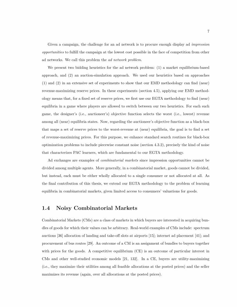
Given a campaign, the challenge for an ad network is to procure enough display ad impression

opportunities to fulfill the campaign at the lowest cost possible in the face of competition from other

ad networks. We call this problem the ad network problem.

We present two bidding heuristics for the ad network problem: (1) a market equilibrium-based

approach, and (2) an auction-simulation approach. We used our heuristics based on approaches

(1) and (2) in an extensive set of experiments to show that our EMD methodology can find (near)

revenue-maximizing reserve prices. In these experiments (section 4.5), applying our EMD method-

ology means that, for a fixed set of reserve prices, we first use our EGTA methodology to find (near)

equilibria in a game where players are allowed to switch between our two heuristics. For each such

game, the designer’s (i.e., auctioneer’s) objective function selects the worst (i.e., lowest) revenue

among all (near) equilibria states. Now, regarding the auctioneer’s objective function as a black-box

that maps a set of reserve prices to the worst-revenue at (near) equilibria, the goal is to find a set

of revenue-maximizing prices. For this purpose, we enhance standard search routines for black-box

optimization problems to include piecewise constant noise (section 4.3.2), precisely the kind of noise

that characterizes PAC learners, which are fundamental to our EGTA methodology.

Ad exchanges are examples of combinatorial markets since impression opportunities cannot be

divided among multiple agents. More generally, in a combinatorial market, goods cannot be divided,

but instead, each must be either wholly allocated to a single consumer or not allocated at all. As

the final contribution of this thesis, we extend our EGTA methodology to the problem of learning

equilibria in combinatorial markets, given limited access to consumers’ valuations for goods.

1.4 Noisy Combinatorial Markets

Combinatorial Markets (CMs) are a class of markets in which buyers are interested in acquiring bun-

dles of goods for which their values can be arbitrary. Real-world examples of CMs include: spectrum

auctions [36] allocation of landing and take-o� slots at airports [15]; internet ad placement [41]; and

procurement of bus routes [29]. An outcome of a CM is an assignment of bundles to buyers together

with prices for the goods. A competitive equilibrium (CE) is an outcome of particular interest in

CMs and other well-studied economic models [21, 132]. In a CE, buyers are utility-maximizing

(i.e., they maximize their utilities among all feasible allocations at the posted prices) and the seller

maximizes its revenue (again, over all allocations at the posted prices).

8

While CEs are a static equilibrium concept, they can sometimes arise as the outcome of a dynamic

price adjustment process (e.g., [32]). In such a process, prices might be adjusted by an imaginary

auctioneer, who poses demand queries to buyers: i.e., asks them their demands at given prices.

Similarly, we imagine that prices in a CM are set by a market maker, who poses value queries to

buyers: i.e., asks them their values on select bundles.

One of the defining features of CMs is that they a�ord buyers the flexibility to express complex

preferences, which in turn has the potential to increase market e�ciency. However, the extensive

expressivity of these markets presents challenges for both the market maker and the buyers. With

an exponential number of bundles in general, it is infeasible for a buyer to evaluate them all. We

thus present a model of noisy buyer valuations: e.g., buyers might use approximate or heuristic

methods to obtain value estimates [45]. In turn, the market maker chooses an outcome in the face

of uncertainty about the buyers’ valuations. We call these markets noisy combinatorial markets

(NCM) to emphasize that buyers do not have direct access to their values for bundles, but instead

can only noisily estimate them.

In this thesis, we formulate a mathematical model of NCMs. Our goal is then to design learning

algorithms with rigorous finite-sample guarantees that approximate the competitive equilibria of

NCMs. First, we present tight lower- and upper-bounds on the set of CE, given uniform approxi-

mations of buyers’ valuations. We then present two learning algorithms. The first one—Elicitation

Algorithm; EA—serves as a baseline. It uses Hoe�ding’s inequality [62] to produce said uniform

approximations. Our second algorithm—Elicitation Algorithm with Pruning; EAP—leverages the

first welfare theorem of economics to adaptively prune value queries when it determines that they

are provably not part of a CE.

After establishing the correctness of our algorithms, we evaluate their empirical performance

using both synthetic unit-demand valuations and two spectrum auction value models. The former

are a class of valuations central to the literature on economics and computation [79], for which

there are e�cient algorithms to compute CE [58]. In the spectrum auction value models, the

buyers’ valuations are characterized by complements, which complicate the questions of existence

and computability of CE. In all three models, we measure the average quality of learned CE via our

algorithms, compared to the CE of the corresponding certain market (i.e., here, “certain” means

lacking uncertainty), as a function of the number of samples. We find that EAP often yields better

error guarantees than EA using far fewer samples, because it successfully prunes buyers’ valuations

9

(i.e., it ceases querying for buyers’ values on bundles of goods that a CE provably does not comprise),

even without any a priori knowledge of the market’s combinatorial structure.

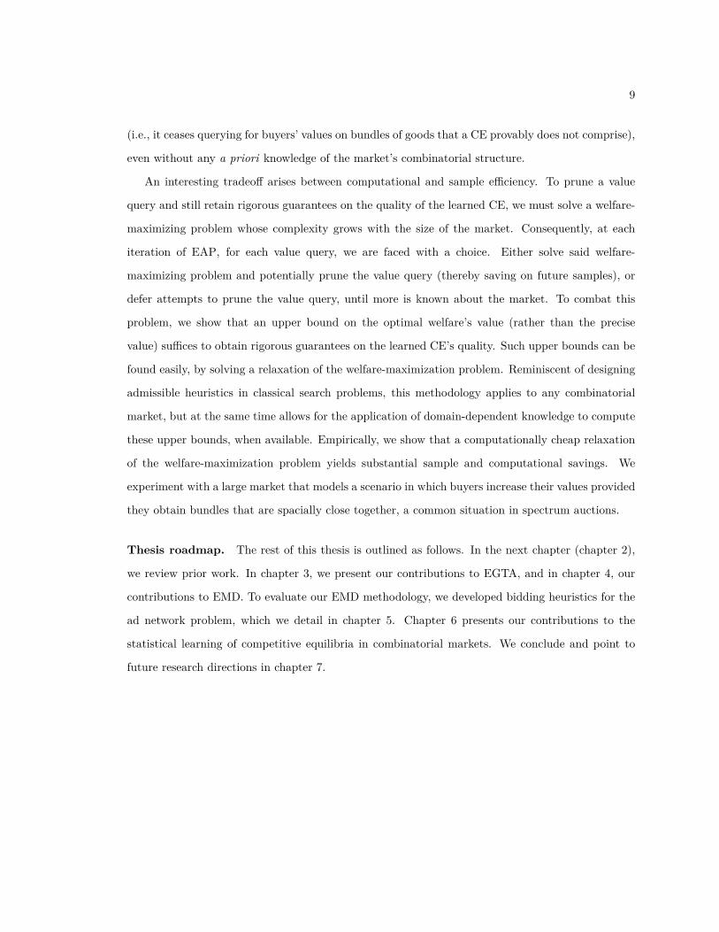
An interesting tradeo� arises between computational and sample e�ciency. To prune a value

query and still retain rigorous guarantees on the quality of the learned CE, we must solve a welfare-

maximizing problem whose complexity grows with the size of the market. Consequently, at each

iteration of EAP, for each value query, we are faced with a choice. Either solve said welfare-

maximizing problem and potentially prune the value query (thereby saving on future samples), or

defer attempts to prune the value query, until more is known about the market. To combat this

problem, we show that an upper bound on the optimal welfare’s value (rather than the precise

value) su�ces to obtain rigorous guarantees on the learned CE’s quality. Such upper bounds can be

found easily, by solving a relaxation of the welfare-maximization problem. Reminiscent of designing

admissible heuristics in classical search problems, this methodology applies to any combinatorial

market, but at the same time allows for the application of domain-dependent knowledge to compute

these upper bounds, when available. Empirically, we show that a computationally cheap relaxation

of the welfare-maximization problem yields substantial sample and computational savings. We

experiment with a large market that models a scenario in which buyers increase their values provided

they obtain bundles that are spacially close together, a common situation in spectrum auctions.

Thesis roadmap. The rest of this thesis is outlined as follows. In the next chapter (chapter 2),

we review prior work. In chapter 3, we present our contributions to EGTA, and in chapter 4, our

contributions to EMD. To evaluate our EMD methodology, we developed bidding heuristics for the

ad network problem, which we detail in chapter 5. Chapter 6 presents our contributions to the

statistical learning of competitive equilibria in combinatorial markets. We conclude and point to

future research directions in chapter 7.

Chapter 2

Prior Work

In this chapter, we first review prior work on empirical game-theoretic analysis, followed by prior

work on empirical mechanism design. Then, we review prior work on electronic advertisement

markets, which serves as our primary application throughout. We conclude with a summary of

literature concerning the learning of competitive equilibria in combinatorial markets.

2.1 Prior Work: Empirical Game-Theoretic Analysis

The EGTA literature, while relatively young, is growing rapidly, with researchers actively con-

tributing methods for myriad game models. Some of these methods are designed for normal-form

games [120, 129], and others, for extensive-form games [49, 84, 142]. Most of these methods ap-

ply to games with finite strategy spaces, but some apply to games with infinite strategy spaces

[84, 131, 140]. Our methodology applies to normal-form games with either finite or infinite strategy

spaces.

We take [134] as our starting point from a methodological point of view. The author proposes

a high-level, architectural view of EGTA made up of three components: (1) parameterization of

strategy spaces, (2) estimation of empirical games, and (3) analysis of empirical games. To illus-

trate the methodology, he deploys it in the Supply Chain Management game of the Trading Agent

Competition (TAC/SCM) game [66]. In this thesis, we present contributions to (2) and (3). An

exciting future research direction is to extend our methodologies to address problems related to the

parameterization of strategy spaces.

10

11

To analyze simulation-based games (component (3)), one first defines a notion of approximate

equilibrium amenable to statistical estimation. Most prior work centers around Á-Nash equilib-

rium [66, 67, 120, 121, 122, 130], an approximation of Nash equilibrium up to an additive error of

Á, following the long-standing tradition of using Nash equilibria as the de facto solution concept to

analyze non-cooperative games [51]. We follow this tradition.

Having defined the notion of equilibria of interest, the search problem is now a combination

of components (2) and (3), where an algorithm both estimates and analyzes an empirical game

simultaneously. The search space in EGTA refers to the space of strategy profiles. Jordan et al. [67]

make the interesting distinction between two models of search: (a) the revealed-utility model, where

each search step determines the exact utility for a designated pure-strategy profile; and (b) the noisy-

utility model, where each search step draws a stochastic sample corresponding to such a utility. Our

work falls into model (b).

Most EGTA methodologies share the same goal, namely, to estimate an equilibrium of the game

(except for a few notable exceptions [121, 128, 139]). In this thesis’ EGTA methodology, we aim to

bound the regret over all equilibria of a simulation-based instead of one equilibrium. Hence, strictly

speaking, we do not directly address the search problem as previously stated. Nonetheless, we tackle

an analogous search problem for our setting. Specifically, our problem is to minimize the number of

queries to the game’s simulator while maintaining robust guarantees over all the game’s equilibria.

Towards this end, we contribute two learning algorithms: global sampling (GS), and progressive

sampling with pruning (PSP). Global sampling uniformly samples all utilities of a simulation-based

game to obtain, with high probability, a desired degree of accuracy. Progressive sampling with

pruning dynamically allocates samples to minimize the number of queries to the game’s simulator.

In contexts other than EGTA, prior art [42, 104, 105] has used progressive sampling to obtain a

desired accuracy given a failure probability by guessing an initial sample size, computing (statistical)

bounds, and repeating with larger sample sizes until said accuracy is attained. Our work applies

this idea to EGTA and complements it with pruning: at each iteration, utilities of strategy profiles

that have already been su�ciently well estimated for the task at hand (here, equilibrium estimation)

are pruned as subsequent iterations of PSP do not refine their bounds. Pruning represents both a

statistical and computational improvement over earlier progressive sampling techniques.

12

Finally, is worth mentioning that EGTA methodologies have been applied in a variety of prac-

tical settings. Some of these include trading agent analyses in supply chains [66, 130, 136], ad

auctions [65], ad exchanges [116, 125], and energy markets [70]; designing network routing proto-

cols [138]; adversarial planning [113]; strategy selection in real-time games [120]; and the dynamics

of RL algorithms, like AlphaGo [121].

2.2 Prior Work: Empirical Mechanism Design

Mechanism design is concerned with the design of games in which the strategic behavior of par-

ticipants leads to desired outcomes. Traditional mechanism design lies within the realm of game

theory, itself an area of economics. Traditionally, a mechanism designer would first manually design

a game, guided by domain-specific expertise, and would then try to prove that the ensuing outcomes

satisfy certain criteria [88]. However, with the advent of strategic autonomous agents, particularly

in e-commerce settings, there has been a surge of interest in computational mechanism design within

the computer science community [38, 91, 96, 115].

In the artificial intelligence community, at least two approaches to mechanism design have

emerged. The first is automated mechanism design [35, 59, 115], where a mechanism is automati-

cally created by an algorithm that searches through a space of mechanisms constrained by standard

mechanism design criteria, such as individual rationality and incentive compatibility. The second is

empirical mechanism design (EMD) [130], where the designer is interested in optimizing a mecha-

nism’s parameters (e.g., reserve prices in auctions) relative to some objective function of interest,

(e.g., revenue), under the assumption of (e.g., Nash) equilibrium play. Crucially, and like in EGTA,

in EMD, we assume no direct access to players’ utilities under di�erent choices of mechanism; we

instead assume access to a simulator capable of producing samples of utilities. One distinguishing

feature of our EMD work vis à vis the existing literature is that we formulate the search for a

mechanism’s optimal parameters as a black-box optimization problem, and then leverage Bayesian

optimization techniques to carry out the search.

13

2.3 Prior Work: Bidding for Electronic Ad Auctions

Our work on bidding heuristics for electronic advertisement markets was initially inspired by the ad

exchange (AdX) game [116], one of many games played as part of the Trading Agent Competition

(TAC) [137], a tournament in which teams of programmers from around the world build autonomous

agents that trade in market simulations. Application domains for these games have ranged from

travel [56] to supply chain management [112] to ad auctions [65] to energy markets [70].

In the TAC AdX game, agents representing ad networks bid to fulfill ad campaigns, which they do

by acquiring opportunities to show impressions to users from di�erent demographics. Bidding repeats

over a series of simulated days, and agents’ reputations for successfully fulfilling past campaigns

impact their ability to procure future campaigns. Our focus is on the ad network problem only: i.e.,

how to bid to most profitably fulfill one campaign. Hence, we define a one-day AdX game, consisting

of only a single simulated day. Nonetheless, ours is a complex game. In the simulation, auctions

are held repeatedly over the course of the day, as users visit web sites. Each such user/impression

opportunity is allocated via a second-price auction with reserve. But agents submit their bids

upfront, and cannot change them over the course of the day. At decision time, agents know only the

distribution and the expected number of users of each demographic, not the particular realizations.

The richness of this game implies that it is unlikely to be solved analytically. Hence, we devise

bidding heuristics for it.

The market induced by the one-day AdX game description has indivisible goods since impression

opportunities are either entirely allocated to an agent or not. One of our bidding heuristics consists of

computing a competitive equilibrium of said market, using it as a prediction for allocation and prices,

and bidding accordingly. The study of competitive equilibria has a long standing tradition, starting

from the seminal work of French economist Léon Walras [132]. In his work, Walras considered

divisible goods, i.e., goods that can be allocated to consumers in fractional amounts. More recently,

authors have extended Walras’ work to markets with multiple, indivisible goods [21, 46, 68]. These

markets are a class of markets where buyers are interested in acquiring packages or bundles of goods.

These markets underlie a variety of mechanisms that are fundamental to modern economies. Some

examples of such mechanisms include: spectrum auctions, of which the 2014 Canadian 700 MHZ

raised upwards of $5 billion [133], allocation of landing and take-o� slots at airports [15], Internet

ad placement [41], procurement of bus routes [29], among others [40, 95].

14

2.4 Prior Work: Noisy Combinatorial Markets

The inspiration for the model of noisy combinatorial markets introduced in this thesis stemmed

from the work on abstraction in Fisher markets by Kroer et al. [74]. There, the authors tackle

the problem of computing equilibria in large markets by creating an abstraction of the market,

computing equilibria in the abstraction, and lifting those equilibria back to the original market.

Likewise, we develop a pruning criterion which in e�ect builds an abstraction of any combinatorial

market. Given this abstraction, we then compute a competitive equilibrium (CE) of it, which we

show is provably also an approximate CE in the original market.

Jha and Zick [64] have also tackled the problem of learning CE in combinatorial markets1.

Whereas our approach is to accurately learn only those components of the buyers’ valuations that

determine a CE (up to PAC guarantees), their approach bypasses the learning of agent preferences

altogether, going straight for learning a solution concept, such as a CE. It is an open question as to

whether one approach dominates the other, in the context of noisy combinatorial markets.

Another related line of research is concerned with learning valuation functions from data [13,

14, 78]. In contrast, our work is concerned with learning buyers’ valuations only in so much as it

facilitates learning CE. Indeed, our main conclusion is that CE often can be learned from just a

subset of the buyers’ valuations.

There is also a long line of work on preference elicitation in combinatorial auctions (e.g., [34]),

where an auctioneer aims to pose value queries in an intelligent order so as to minimize the compu-

tational burden on the bidders, while still clearing the auction.

Whereas intuitively, a basic pruning criterion for games is arguably more straightforward—simply

prune dominated strategies—the challenge in this case was to discover a pruning criterion that would

likewise prune valuations that are provably not part of a CE. Our pruning criterion relies on a novel

application of the first welfare theorem of economics. While prior work has connected economic the-

ory with algorithmic complexity [110], this work connects economic theory with statistical learning

theory.

1The market structure they investigate is not identical to the structure studied here. Thus, at present, our results

are not directly comparable.

Chapter 3

Empirical Game-Theoretic

Analysis

In this chapter, we present our contributions to the empirical game-theoretic analysis literature.

The contents of this chapter are an extended version of the following published papers: Learn-

ing Simulation-Based Games from Data [7] (arXiv version Learning Equilibria of Simulation-Based

Games [6]), and Improved Algorithms for Learning Equilibria in Simulation-Based Games [8].

3.1 Game Theory Background

We first o�er some necessary background on game theory. Central to our work is the fundamental

notion of a normal-form game, which we formally define next.

Definition 1 (Normal-form game)

A normal-form game � .= ÈP, {Sp | p œ P}, u(·)Í consists of a finite set of agents P , with pure

strategy set Sp available to agent p œ P . We define S.= S1 ◊ · · · ◊ S|P | to be the pure strategy

profile space of �, and then u : S æ R|P | is a vector-valued utility function (equivalently, a

vector of |P | scalar utility functions up).

Given a normal-form game �, we let Sùp denote the set of distributions over Sp; this set contains

p’s mixed strategies. We define Sù = Sù1 ◊ · · · ◊ S

ù|P |, and then, overloading notation, we write u(s)

15

16

to denote the expected utility of a mixed strategy profile s œ Sù.

A solution to a normal-form game is a prediction of how strategic agents will play the game. One

solution concept that has received a great deal of attention in the literature is Nash equilibrium [90],

a (pure or mixed) strategy profile at which each agent selects a utility-maximizing strategy, fixing all

other agents’ strategies. In our work, we are concerned with Á-Nash equilibrium, an approximation

of Nash equilibrium that is amenable to statistical estimation.

Given a game �, fix an agent p and a mixed strategy profile s œ Sù. Let T ùp,s be the set of all

mixed strategy profiles in which the strategies of all agents q ”= p are fixed at sq. Mathematically,

T ùp,s

.= {t œ Sù| tq = sq, ’q ”= p}.

Definition 2 (Regret)

Given a game � with utility u, fix an agent p and a mixed strategy profile s œ Sù. We

define Adjùp,s.= {t œ Sù

| tq = sq, ’q ”= p}. In words, Adjùp,s is the set of adjacent mixed

strategy profiles: i.e., those in which the strategies of all agents q ”= p are fixed at sq. Agent p’s

regret at s is defined as: Regùp(u, s) .= supsÕœAdjù

p,sup(sÕ) ≠ up(s). By restricting s and Adjùp,s

to pure strategy profiles, agent p’s pure regret Regp(u, s) can be defined similarly, with respect

to Adjp,s.

Note that Regùp(u, s), Regp(u, s) Ø 0, since agent p can deviate to any strategy s

Õœ Sp, including

sp itself. A strategy profile s that has regret at most Á Ø 0, for all p œ P , is an Á-Nash equilibrium:

Definition 3 (Á-Nash equilibrium)

Given Á Ø 0, a mixed strategy profile s œ Sù in a game � is an Á-Nash equilibrium if,

for all p œ P , Regùp(u, s) Æ Á. At a pure strategy Á-Nash equilibrium s œ S, for all p œ P ,

Regp(u, s) Æ Á. We denote by EùÁ(u) the set of mixed Á-Nash equilibria, and by EÁ(u), the set

of pure Á-Nash equilibria. Note that EÁ(u) ™ EùÁ(u).

3.2 A Framework for EGTA

Our first contribution towards a complete framework for EGTA is to show that the equilibria of a

game can be approximated with bounded error, given only a uniform approximation of the game’s

17

utility functions. Specifically, our theorem establishes perfect recall1: the approximate game contains

all true positives: i.e., all (exact) equilibria of the original game. It also establishes approximately

perfect precision: all false positives in the approximate game are approximate equilibria in the

original game.

Building towards this result, we first define the metric by which we will measure the error between

games, i.e., the ¸Œ-norm. The error measurement holds only between games with the same agents

sets P and strategy profile spaces, but whose utilities functions are not necessarily the same. We

call such games compatible games. Later on, we will see that associated with a ground-truth game

(whose utility functions we do not get to observe), there are empirical games (whose utility functions

we get to observe via samples). An empirical game is compatible with its ground-truth counterpart,

and thus, it makes sense to measure the error between them.

Definition 4 (¸Œ-norm of games)

We define the ¸Œ-norm between two compatible games, with the same agents sets P and

strategy profile spaces S, and with utility functions u, uÕ, respectively, as follows:

Î� ≠ �ÕÎŒ

.= Îu(·) ≠ uÕ(·)ÎŒ.= sup

pœP,sœS|up(s) ≠ uÕ

p(s)|

While the Œ-norm as defined applies only to pure normal-form games, it is in fact su�cient to

use this metric even to show that the utilities of mixed strategy profiles approximate one another.

We formalize this claim in the next lemma.

Lemma 1 (Approximations in Mixed Strategies). If �, �Õ are compatible games, i.e., they di�er

only in their utility functions, u, uÕ, then

suppœP,sœSù

|up(s) ≠ uÕp(s)| = Î� ≠ �Õ

ÎŒ

Proof. For any agent p and mixed strategy profile t œ Sù, up(t) =q

sœS t(s)up(s), where t(s) =r

pÕœP tpÕ(spÕ). So, up(t) ≠ uÕp(t) =

qsœS t(s)(up(s) ≠ uÕ

p(s)) Æ supsœS |up(s) ≠ uÕp(s)|, by Hölder’s

inequality. Hence, suptœSù |up(t) ≠ uÕp(t)| Æ supsœS |up(s) ≠ uÕ

p(s)|, from which it follows that1We use the term recall in the information retrieval sense. The juxtaposition of the two words “perfect” and

“recall” is not a reference to extensive-form games.

18

suppœP,tœSù |up(t) ≠ uÕp(t)| Æ Î� ≠ �Õ

ÎŒ. Equality holds for any p and s that realize the supremum

in Î� ≠ �ÕÎŒ, as any such pure strategy profile is also mixed.

Central to our work is the notion of uniform Á-approximation between games. We make this

notion precise in the next definition.

Definition 5 (Á-Uniform approximation of games)

�Õ is said to be a uniform Á-approximation of � when Î� ≠ �ÕÎŒ Æ Á.

In an Á-uniform approximation of �Õ by �, the bound between utility deviations in �Õ and �

(and, symmetrically, in � and �Õ) holds uniformly over all players and strategy profiles. Hence

the name uniform approximation. We can now present our theorem that characterizes the approx-

imation guarantees on the set of Nash equilibria of a game given an Á-uniform approximation of

it. Looking ahead, we rely on this theorem to show good approximations between simulation-based

games (definition 7) and their empirical counterparts (definition 8).

Theorem 1 (Approximate Equilibria). Given normal-form games �, �Õ, with utility functions u

and uÕ, respectively, such that Î� ≠ �ÕÎ Œ Æ Á, the following hold:

1. E(u) ™ E2Á(uÕ) ™ E4Á(u), and

2. Eù(u) ™ Eù2Á(uÕ) ™ Eù

4Á(u).

Proof. First note the following: if A ™ B, then C fl A ™ C fl B. Hence, since any pure Nash equilib-

rium is also a mixed Nash equilibrium, taking C to be the set of all pure strategy profiles, we need

only show 2. We do so by showing Eù“(u) ™ Eù

2Á+“(uÕ), for “ Ø 0, which implies both containments,

taking “ = 0 for the lesser, and “ = 2Á for the greater.

Suppose s œ Eù“(u), for all p œ P . We will show that s is (2Á + “)-optimal in �Õ, for all p œ P .

Fix an agent p, and recall Adjùp,s.= {t œ Sù

| tq = sq, ’q ”= p}. Now take súœ arg maxtœAdjù

p,sup(t)

and sÕúœ arg maxtœAdjù

p,suÕ

p(t). Then:

Regùp(uÕ

, s) = uÕp(sÕú) ≠ uÕ

p(s)

Æ (up(sÕú) + Á) ≠ (up(s) ≠ Á)

Æ (up(sú) + Á) ≠ (up(s) ≠ Á)

Æ (up(sú) + Á) ≠ (up(sú) ≠ Á ≠ “) = 2Á + “

19

The first line follows by definition. The second holds by Lemma 1 and the fact that �Õ is a uniform

Á-approximation of �, the third as sú is optimal for p in �, and the fourth as s is a “-Nash in �.

We note that part of this theorem was concurrently proved by other researchers [121], albeit in

a di�erent formalism than ours. We now briefly explain their results in the language of our work.

They showed the set containment E(u) ™ E2Á(uÕ). We complement this result by further observing

that E2Á(uÕ) ™ E4Á(u). We also provide a machine learning interpretation in the language perfect

recall and approximately perfect precision.

3.2.1 Learning Framework

We move on from approximating equilibria in games to learning them. We first present a learning

framework where we define our model of simulation-based games (definitions 6 and 7). We then define

empirical games (definition 8) which are the games we ultimately get to observe by sampling a game’s

simulator. In the next section, we present algorithms that learn so-called empirical games, which

comprise estimates of the expected utilities of simulation-based games. We further derive uniform

convergence bounds, PAC-style guarantees proving that our algorithms output empirical games

that uniformly approximate their expected counterparts, with high probability. By Theorem 1, the

equilibria of these empirical games thus approximate those of the corresponding simulation-based

games, with high probability.

Definition 6 (Conditional Normal-Form Game)

A conditional normal-form game �X.= ÈX , P, {Sp | p œ P}, u(·)Í consists of a set of condi-

tions X , a set of agents P , with pure strategy set Sp available to agent p, and a vector-valued

conditional utility function u : S ◊ X æ R|P |.

In the definition above, it is convenient to imagine a condition x œ X as pertaining to the set

P ◊S. Given such a condition, u(·; x) yields a standard utility function of the form S æ R|P |, which

evaluates as usual, returning the vector u(s; x) when given a strategy profile s œ S.

Associated with a conditional normal-form game, we define, for a fixed distribution D over

condition set X , its corresponding expected normal-form game as follows. Finally, we define the

empirical normal-form games, which are games obtained by drawing samples from X .

20

Definition 7 (Expected Normal-Form Game)

Given a conditional normal-form game �X together with distribution D , we also define

the expected utility function u(s; D) = Ex≥D [u(s; x)], and the expected normal-form game as

�D.= ÈP, {Sp | p œ P}, u(·; D)Í.

Definition 8 (Empirical Normal-Form Game)

Given a conditional normal-form game �X together with a distribution D from which we

can draw sample conditions X = (x1, . . . , xm) ≥ Dm, we define the empirical utility function

u(s; X) .= 1m

qmj=1 u(s; xj).

The corresponding empirical normal-form game is then �X.= ÈP, {Sp | p œ P}, u(·; X)Í.

Together, conditional and expected normal-form games constitute our mathematical model of

simulation-based games. In a simulation-based game, players’ utilities depend not only on the

strategies at play but also on unobserved exogenous elements, often stochastic. Abstractly, we model

these elements condition set X that, together with the chosen strategies2, defines the corresponding

conditional normal-form game. By repeatedly querying a simulator, we observe samples of utilities

that then form an empirical normal-form game. Our goal is to approximate, from empirical normal-

form games, the equilibria of the corresponding expected normal-form game for fixed distribution

D over condition set X . The expected normal-form game resolves all uncertainty and thus, serves

as our ground-truth game for strategic analysis.

The following simple example illustrates our mathematical model of simulation-based games.

Example 1 (Conditional, Expected, and Empirical Normal-Form Game)

Consider the following simplified version of the diner’s dilemma gamea. You and your

friend decide to go out to eat together. Since you are friends (and maybe a bit careless!), you

decide, before ordering, to split the bill in half. To keep this example simple, suppose that

your restaurant of choice o�ers only two options: a cheap dish that costs $2 and an expensive

dish that costs $8. You and your friend grew up together, so naturally, you have similar tastes.

2In this thesis, we assume a fixed set of strategies is given to us prior to any strategic analysis. This condition holds

in meta-games like Starcraft [121], for example, where agents choices comprise a few high-level heuristic strategies,

not intractably many low-level game-theoretic strategies.

21

In particular, you both share the same (monetary) values of $5 and $10 for the cheap and

expensive dish, respectively. In this example, the utility associated with a dish is the value of

the dish minus the payment, i.e., half the bill for the entire meal.

Given that both you and your friends are utility-maximizing agents, the central strategic ques-

tion now is: what dish should you (your friend) choose considering what your friend (you)

might choose? To help us answer this question, we can write the normal-form game that mod-

els this strategic situation. Let C denote the choice of a cheap dish and E the choice of an

expensive dish. If both you and your friend chose a cheap dish, then each receives utility 3,

u(C, C) = [5 ≠ (2 + 2) / 2, 5 ≠ (2 + 2) / 2] = [3, 3]. If you both chose expensive meals,

then each receives 2, u(E, E) = [10 ≠ (8 + 8) / 2, 10 ≠ (8 + 8) / 2] = [2, 2]. Finally, if the

choices are not the same, the cost of half the bill is (2 + 8) / 2 = 5, which means that whoever

chose the cheap dish receives 0 utility and the other 5, u(C, E) = [5 ≠ 5, 10 ≠ 5] = [0, 5].

The following table summarizes the utility of all possible choices of meals in this game.

C E

C 3, 3 0, 5

E 5, 0 2, 2

Table 3.1: Bimatrix for the diner’s dilemma game.

Note that the table above completely characterizes the game you and your friend face, given

that both of you have perfect information about all essential elements to make a decision. The

reader can verify that the game’s unique 0-Nash equilibrium is when both players chose to

order the expensive dish. In this case, both make a utility of 2. However, a higher-utility state

for both agents would be when both chose the cheap dish, but alas, the incentives are so that

choosing the expensive deal is a better strategic choice. Hence, each player faces a dilemma

between choosing the cheap dish and hoping their friend does the same, thereby maximizing

both of their utilities; or following the strictly rational choice and selecting the expensive dish

to maximize its own utility regardless of its friend choice.

22

But now, suppose that the situation complicates slightly. It is still the case that you (and your

friend) value the expensive dish at $10, but only when the restaurant’s cook is in a good mood.

In this case, the cook puts all his e�orts into making the expensive dish, resulting in a delicious

meal. Otherwise, if the cook is not in a good mood, he spends less e�ort preparing itb, and the

result is not so delicious. In this case, your (and your friend’s) value for the dish drops to $8.

Since the cheap dish is much easier to prepare, your value for the cheap dish remains at $5,

regardless of the cook’s mood. The cost of both dishes is the same as beforec. We can model

the conditional normal-form associated with this situation as follows.

Define set of conditions X = {Good Mood, Bad Mood}. The conditional utility function is

then given by u(C, C; Good Mood) = u(C, C; Bad Mood) = u(C, C) = [3, 3], in case both

chose the cheap dish. In case they both choose the expensive dish, u(E, E; Good Mood) =

u(E, E) = [2, 2], and u(E, E; Bad Mood) = [8 ≠ (8 + 8)/ 2, 8 ≠ (8 + 8)/ 2] = [0, 0].

Note that, in this case, the players’ utilities depend not only on the players’ choices but also

on the (possibly unobserved) cook’s mood. Finally, if you go with the cheap dish while your

friend goes with the expensive cheap, then u(C, E; Good Mood) = u(C, E) = [0, 5] and

u(C, E; Bad Mood) = [5 ≠ 5, 8 ≠ 5] = [0, 3]. This completely defines the conditional

normal-form game.

How should you decide what to do in this more complicated situation? Suppose that your

decision complicates by the fact that you can’t tell precisely the mood of the cook. However,

you might have observed (say, from past visits to the restaurant) that the cook is in a good mood

most of the time. Your goal is to make a good strategic decision most of the time (say, on future

visits with your friend to the restaurant). In that case, we can further model your lack of certain

knowledge about the cook’s mood by positing the existence of distribution, D , over the cook’s

mood. For example, suppose that your observations indicate that PrD(Good Mood) = 3/4

and PrD(Bad Mood) = 1/4. Given this information, we can model the expected normal-

form game as the game whose utilities are given by taking expectations of the corresponding

conditional normal-form game’s utilities over D . For example, let us compute the utility of the

expected normal-form game in case you and your friend chose the expensive dish:

23

u(E, E; D) = Ex≥D

[u(E, E; x)]

= 3/4u(E, E; Good Mood) + 1/4u(E, E; Bad Mood)

= 3/4[2 , 2] + 1/4[0, 0]

= [3/2 , 3/2]

(3.1)

The reader can verify that computing utilities for all strategies profiles yields the following

expected-normal form game,

C E

C 3, 3 0, 9/2

E 9/2, 0 3/2, 3/2

Table 3.2: Bimatrix for the expected normal-form diner’s dilemma game

Estimating the equilibria of the above game is our EGTA methodology’s goal. This goal would

reduce to a purely computational problem if we had access to the bimatrix above. Note,

however, that per our setup, we never get to observe said bimatrix. In fact, in most cases of

practical importance, we never get to observe neither X nor D . Instead, we only get to observe

utility samples that we can collect into empirical normal-form games. In the case of your choice

of meal, samples might come from multiple visits to the restaurant where both you and your

friend select a dish, pay the bill, and measure your utilities. In practice, samples come from a

game’s simulator.aA diner’s dilemma game can also be understood as a n-player prisoner’s dilemma game [94].

bBeing angry requires some e�ort!

cThe restaurant would be wise then to keep the cook in a good mood!

Having established our learning framework, our present goal, then, is to “uniformly learn” empir-

ical games (i.e., obtain uniform convergence guarantees) from finitely many samples. This learning

problem is non-trivial because it involves multiple comparisons. Tuyls et al. [121] use Hoe�ding’s

inequality to estimate a single utility value, and then apply a äidák correction to estimate all utility

values simultaneously, assuming independence among agents’ utilities. Similarly, one can apply a

Bonferroni correction (i.e., a union bound) to Hoe�ding’s inequality, which does not require inde-

pendence, but yields a slightly looser bound.

24

Theorem 2 (Finite-Sample Bounds via Hoe�ding’s Inequality). Consider finite, conditional normal-

form game �X together with distribution D and index set I ™ P ◊ S such that for all x œ X and

(p, s) œ I, it holds that up(s; x) œ [≠c/2, c/2], where c œ R. Then, with probability at least 1 ≠ ” over

X ≥ Dm, it holds that

sup(p,s)œI

|up(s; D) ≠ up(s; X)| Æ c

Ûln( 2|I|

” )2m

Proof. By Hoe�ding’s inequality [62],

Pr(|up(s; D) ≠ up(s; X)| Ø Á) Æ 2e≠2m

1Á

c

22

(3.2)

Now, applying union bound over all events |up(s; D) ≠ up(s; X)| Ø Á where (p, s) œ I,

Pr

Q

a€

(p,s)œI

|up(s; D) ≠ up(s; X)| Ø Á

R

b Æ

ÿ

(p,s)œI

Pr (|up(s; D) ≠ up(s; X)| Ø Á) (3.3)

Using bound (3.2) in the right-hand side of (3.3),

Pr

Q

a€

(p,s)œI

|up(s; D) ≠ up(s; X)| Ø Á

R

b Æ

ÿ

(p,s)œI

2e≠2m( Á

c )2= 2|I|e

≠2m

1Á

c

22

(3.4)

Where the last equality follows because the summands on the right-hand size of eq. (3.4) do not

depend on the summation index. Now, note that eq. (3.4) implies a lower bound for the event that

complementst

(p,s)œI |up(s; D) ≠ up(s; X)| Ø Á,

Pr

Q

a€

(p,s)œI

|up(s; D) ≠ up(s; X)| Æ Á

R

b Ø 1 ≠ 2|I|e≠2m

1Á

c

22

(3.5)

The eventu

(p,s)œI |up(s; D) ≠ up(s; X)| Æ Á is equivalent to the event max(p,s)œI |up(s; D) ≠

up(s; X)| Æ Á. Setting ” = 2|I|e≠2m( Á

c )2 and solving for Á yields Á = c

ln(2|I|/”)/2m.

The results follows by substituting Á in eq. (3.5).

Remark Given a game, we state all theorems and algorithms for an arbitrary index set I. Taking

I = P ◊ S, we bound Îu(·; D) ≠ u(·; X)ÎŒ.

25

Consider X1:m independent and identically distributed random variables, and their mean X. (In

our case, Xj = u(s; xj).) Hoe�ding’s inequality for bounded random variables can be used to obtain

tail bounds on the probability that an empirical mean di�ers greatly from its expectation. One way

to characterize such bounds is to compare them to well-studied cases of common random variables.

We focus on the case of upper tails, as we apply only symmetric two-tail bounds in this work.

Random variables that obey the Gaussian Cherno� bound can be characterized as ‡2N -sub-

Gaussian: i.e.,

Pr!X Ø E[X] + Á

"Æ exp

3≠mÁ

2

2‡2N

4≈∆ Pr

AX Ø E[X] +

Ú2‡

2N ln( 1

” )m

BÆ ”

Here, ‡2N is deemed a variance proxy. Using this characterization, Hoe�ding’s inequality reads “If

Xi has range c, then Xi is c2/4-sub-Gaussian,” because, by Popoviciu’s inequality [101], V[Xi] Æ c2

/4.

Thus, Hoe�ding’s inequality yields sub-Gaussian tail bounds.

This result is not entirely satisfying, however, as it is stated in terms of the worst-case variance;

when V[Xi] π c2/4, tighter bounds should be possible. We might hope that knowledge of the

variance ‡2 would imply ‡

2-sub-Gaussian, but it does not; taking the range c to Œ allows Xi to

exhibit arbitrary tail behaviors. A (‡2�, c)-sub-gamma [27] random variable obeys

Pr

AX Ø E[X] +

c ln( 1” )

3m+

Ú2‡

2� ln( 1

” )m

BÆ ”

While the form of such bounds is more complicated than in the sub-Gaussian case, there is an

intuitive interpretation of the tail behavior as sample size increases. The key is to observe that

the additive error consists of a hyperbolic c ln( 1” )/3m term and a root-hyperbolic

2‡

2N ln( 1

” )/m

term, which in learning theory are often called fast and slow terms, respectively. Sub-gamma

random variables then yield mixed convergence rates, which initially decay quickly while the c-term

dominates, before slowing to the root-hyperbolic rate when the ‡2N term comes to dominate.

Bennett’s inequality 1962, while usually stated as a sub-Poisson bound, immediately implies

that if Xi has range c and variance ‡2, then Xi is (‡2

, c)-sub-gamma. Bennett’s inequality, how-

ever, assumes the range and variance are known. Various empirical Bennett bounds have been

shown [10, 11, 85], which all essentially operate by bounding the variance of a random variable

in terms of its empirical variance and range, and then applying Bennett’s inequality. Simply put,

26

Bennett’s inequality gives us Gaussian-like tail bounds, where the scale-dependent term acts as

an asymptotically negligible correction for working with non-Gaussian distributions and empirical

estimates of variance. Asymptotic central-limit-theorem bounds behave similarly, but lack corre-

sponding finite-sample guarantees.

Our work di�ers from previous applications in that we require confidence intervals of uniform

width, and thus our bounds are limited by the maximum variance over all parameters being estimated.

The maximum variance over a set of random variables is known as the wimpy variance [27]. We

apply a sub-gamma bound to the wimpy variance in terms of an empirical estimate, and then

apply Bennett’s inequality to the upper and lower tails of each utility function using the wimpy

variance bound, as this, by definition, upper bounds the variance of each utility. This strategy yields

uniform-width confidence intervals over all utilities, and requires a union bound over m upper tails,

m lower tails, and the wimpy variance, whereas bounding each variance separately would require a

union bound over m upper, m lower, and m variance bounds. Thus, our method outperforms such

strategies, yielding tighter confidence intervals.

We now present a novel concentration inequality that combines both Hoe�ding’s and Bennett’s

inequalities3.

Theorem 3 (Bennett-Type Variance-Sensitive Finite-Sample Bounds). Suppose as in Theorem 2.

Takev

.= sup(p,s)œI

1m ≠ 1

mÿ

j=1(up(s; xj) ≠ up(s; X))2 ;

Áv.=

c ln( 3” )

m ≠ 1 +

Û1

c ln( 3” )

m ≠ 1

22+

2v ln( 3” )

m ≠ 1 ; and

Áµ.= min

Ac

Ûln( 3|I|

” )2m¸ ˚˙ ˝

Hoeffding

,c ln( 3|I|

” )3m

+

Û2(v + Áv) ln( 3|I|

” )m¸ ˚˙ ˝

Empirical Bennett

B.

Then, with probability at least 1 ≠ ” over X ≥ Dm, it holds that

sup(p,s)œI

|up(s; D) ≠ up(s; X)| Æ Áµ .

3This inequality is the sole contribution of fellow Ph.D. student Cyrus Cousins and its proof can be found in

https://github.com/eareyan/pysegta.

https://github.com/eareyan/pysegta

27

From the definition of Áµ, we see that when v is ¥c2

4 (near-maximal), the Hoeffding term

applies, so this bound matches Theorem 2 to within constant factors (in particular, ln( 3|I|” ) instead

of ln( 2|I|” )). On the other hand, when v is small, Theorem 3 is much sharper than Theorem 2. A

few simplifying inequalities yield

Áµ Æ7c ln( 3|I|

” )3(m ≠ 1) +

Û2v ln( 3|I|

” )m

which matches the standard sub-gamma Bennett’s inequality up to constant factors, with dependence

on v instead of v. In the extreme, when v ¥ 0 (i.e., the game is near-deterministic), then Theorem 3

improves asymptotically over Theorem 2 by a �(Ò

ln( |I|” )/m) factor.

3.2.2 Learning Algorithms

We are now ready to present our algorithms. Specifically, we discuss two Monte-Carlo sampling-

based algorithms that can be used to uniformly learn empirical games, and hence ensure that the

equilibria of the games they are learning are accurately approximated with high probability. Note

that our algorithms apply only to finite games, as they require an enumeration of the index set I.

A conditional normal form game �X , together with distribution D , serves as our mathematical

model of a simulator from which the utilities of a simulation-based game can be sampled. Given

strategy profile s, we assume the simulator outputs a sample up(s, x), for all agents p œ P , after

drawing a single condition value x ≥ D .

Our first algorithm, global sampling (GS), is a straightforward application of Thms. 2 and 3. The

second, progressive sampling with pruning (PSP), is a progressive-sampling-based approach [104,

105], which iteratively prunes strategies, and thereby has the potential to expedite learning by

obtaining tighter bounds than GS, given the same number of samples. We explore PSP’s potential

savings in our experiments, Section 3.3.

GS (Algorithm 1), samples all utilities of interest, given a sample size m and a failure probability

”, and returns the ensuing empirical game together with an Á determined by either Thm. 2 or 3 that

guarantees an Á-uniform approximation.

More specifically, GS takes in a conditional game �X , a black box from which we can sample

distribution D , an index set I ™ P ◊ S, a sample size m, a utility range c such that utilities are

required to lie in [≠c/2, c/2], and a bound type Bd, and then draws m samples to produce an empirical

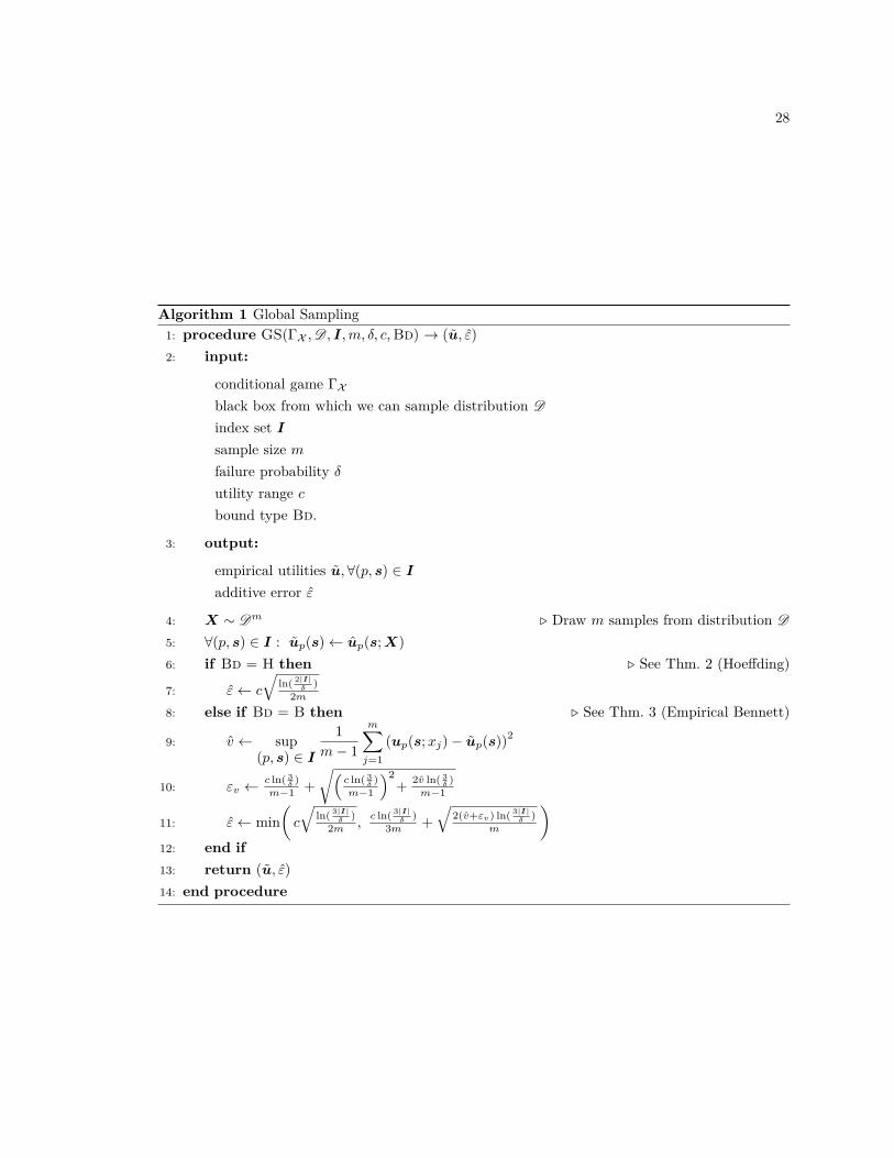
28

Algorithm 1 Global Sampling1: procedure GS(�X , D , I, m, ”, c, Bd) æ (u, Á)2: input:

conditional game �X

black box from which we can sample distribution D

index set I

sample size m

failure probability ”

utility range c

bound type Bd.

3: output:

empirical utilities u, ’(p, s) œ I

additive error Á

4: X ≥ DmÛ Draw m samples from distribution D

5: ’(p, s) œ I : up(s) Ω up(s; X)6: if Bd = H then Û See Thm. 2 (Hoe�ding)

7: Á Ω c

Òln( 2|I|

” )2m

8: else if Bd = B then Û See Thm. 3 (Empirical Bennett)

9: v Ω sup(p, s) œ I

1m ≠ 1

mÿ

j=1(up(s; xj) ≠ up(s))2

10: Áv Ωc ln( 3

” )m≠1 +

Ú1c ln( 3

” )m≠1

22+ 2v ln( 3

” )m≠1

11: Á Ω min3

c

Òln( 3|I|

” )2m ,

c ln( 3|I|” )

3m +Ò

2(v+Áv) ln( 3|I|” )

m

4

12: end if13: return (u, Á)14: end procedure

29

game �X , represented by u(·), as well as an additive error Á, with the following guarantee:

Theorem 4 (Approximation Guarantees of Global Sampling). Consider conditional game �X to-

gether with distribution D and take index set I ™ P ◊ S such that for all x œ X and (p, s) œ I,

up(s; x) œ [≠c/2, c/2], for some c œ R.

If GS(�X , D , I, m, ”, c, Bd) outputs pair (u, Á), then with probability at least 1 ≠ ”, it holds that

sup(p,s)œI

|up(s; D) ≠ up(s)| Æ Á .

Proof of Theorem 4. Use Theorem 2 when Bound = Hoeffding and Theorem 3 when Bound =

Bennett.

Next, we present PSP (Algorithm 2), which, using GS as a subroutine, draws progressively

larger samples, refining the empirical game at each iteration, and stopping when the equilibria

are approximated to the desired accuracy, or when the sampling budget is exhausted. Although

performance ultimately depends on a game’s structure, PSP can potentially learn equilibria using

vastly fewer resources than GS.

As the name suggests, PSP is a pruning algorithm. The key idea is to prune (i.e., cease estimating

the utilities of) strategy profiles that (w.h.p.) are provably not equilibria. Recall that s œ EÁ(u) if

and only if Regp(u, s) Æ Á, for all p œ P . Thus, if there exists p œ P such that Regp(u, s) > Á, then

s ”œ EÁ(u). In the search for pure equilibria, such strategy profiles can be pruned.

A strategy s œ Sp is said to Á-dominate another strategy sÕ

œ Sp if for all s œ S, taking

sÕ = (s1, . . . , sp≠1, sÕp, sp+1, . . . , s|P |), it holds that up(s) ≠ Á Ø up(sÕ). Given a game � with utility

function u, the Á-rationalizable strategies RatÁ(u) are those that remain after iteratively removing all

Á-dominated strategies. This set can easily be computed via the iterative elimination of Á-dominated

strategies. Only strategies in RatÁ(u) can have nonzero weight in a mixed Á-Nash equilibrium [51];

thus eliminating strategies not in RatÁ(u) is a natural pruning criterion for mixed equilibria.

If a strategy s œ Sp is Á-dominated by another strategy sÕ

œ Sp, then p always regrets playing

strategy s, regardless of other agents’ strategies. Consequently, the mixed pruning criterion is more

conservative than the pure, which means more pruning occurs when learning pure equilibria.

Like GS, PSP takes in a conditional game �X , a black box from which we can sample distribution

D , a utility range c, and a bound type Bd. Instead of a single sample size, however, it takes in a

30

sampling schedule M in the form of a (possibly infinite) strictly increasing sequence of integers; and

instead of a single failure probability, it takes in a failure probability schedule ”, with each ”t in this

sequence and their sum in (0, 1). These two schedules dictate the number of samples to draw and

the failure probability to use at each iteration. PSP also takes in a boolean Pure that indicates

whether the equilibria of interest are pure or mixed, and an error threshold Á, which enables early

termination as soon as equilibria of the desired sort are estimated to within the additive factor Á.

Algorithm 2 Progressive Sampling with Pruning1: procedure PSP(�X , D , M , ”, c, Bd, Pure, Á) æ ((u, Á), (E, Á), ”)2: input:

conditional game �X

black box from which we can sample distribution D

sampling schedule M

failure probability schedule ”

utility range c

bound type Bdequilibrium type Pureerror threshold Á

3: output:

Empirical utilities u, ’(p, s) œ P ◊ S

utility error Á

empirical equilibria E

equilibria error Á


4: I Ω P ◊ S Û Initialize index set5: ’(p, s) œ I : (up(s), Áp(s)) Ω (0, c/2), Û Initialize outputs6: for t œ 1, . . . , |M | do Û Progressive sampling iterations7: (u, Á) Ω GS(�X , D , I, Mt, ”t, c, Bd) Û Improve utility estimates8: ’(p, s) œ I : Áp(s) Ω Á Û Update confidence intervals9: if Á Æ Á or t = |M | then Û Termination condition

10: E Ω

IPure : E2Á(u)

¬Pure : Eù2Á(u)

11: return ((u, Á), (E, Á),qt

i=1 ”i)12: end if

13: I Ω

IPure : {(p, s) œ I | Regp(u, s) Æ 2Á}

¬Pure : {(p, s) œ I | ’q œ P : sq œ Rat2Á(u)}14: end for15: end procedure

31

Theorem 5 (Approximation Guarantees of Progressive Sampling with Pruning). Suppose condi-

tional game �X and distribution D such that for all x œ X and (p, s) œ P ◊ S, up(s; x) œ [≠c/2, c/2]

for some c œ R. If PSP(�X , D , M , ”, c, Bd, Pure, Á) outputs!(u, Á), (E, Á), ”

", it holds that:

1. ” Æq

”tœ” ”t, ” œ (0, 1)

2. If limtæŒ ln(1/”t)/Mt = 0, then Á Æ Á.

Furthermore, if PSP terminates, then with probability at least 1 ≠ ”, the following hold simultane-

ously:

3. |up(s; D) ≠ up(s)| Æ Áp(s), for all (p, s) œ P ◊ S

4. If Pure, then E(u) ™ E2Á(u) ™ E4Á(u)

5. If ¬Pure, then Eù(u) ™ Eù2Á(u) ™ Eù

4Á(u).

Proof of Theorem 5. To see 1, note that ” is computed on line 11 as a partial sum of ”, each addend

and the sum of which are all by assumption on (0, 1); thus the result holds.

To see 2, note that if limtæŒ ln(1/”t)/Mt = 0, then both the Hoe�ding’s and Bennett’s bounds

employed by GS tend to 0, as both decay asymptotically (in expectation) as O(

ln(1/”t)/Mt) (see

Theorems 2 and 3). For infinite sampling schedules, the termination condition of line 9 (Á Æ Á) is

eventually met, as Á is the output of GS, and thus 2 holds.

To establish 3, we show the following: assuming termination occurs at timestep n, with proba-

bility at least 1 ≠ ”, at every t in {1, . . . , n}, it holds that sup(p,s)œP ◊S |up(s; D) ≠ up(s)| Æ Áp(s).

This property follows from the GS guarantees of Theorem 4, as at each timestep t, the guarantee

holds with probability at least 1 ≠ ”t; thus by a union bound, the guarantees hold simultaneously

at all time steps with probability at least 1 ≠qn

i=1 ”t = 1 ≠ ”. That the GS guarantees hold for

unpruned indices should be clear; for pruned indices, since only error bounds for indices updated on

line 7 are tightened on line 8, it holds by the GS guarantees of previous iterations.

Without pruning, 4 and 5 would follow directly from 3 via Theorem 1, but with pruning, the

situation is a bit more involved. To see 4, observe that at each time step, only indices (p, s) such

that Regp

!u(·), s

"> 2Á are pruned (line 13), thus we may guarantee that with probability at least

1 ≠ ”, Regp

!u(·; D), s

"> 0. Increasing the accuracy of the estimates of these strategy profiles is

thus not necessary, as they do not comprise pure equilibria (w.h.p.), and they will never be required

to refute equilibria, as these will never be a best response for any agent from any strategy profile.

32

5 follows similarly, except that nonzero regret implies that a pure strategy profile is not a pure

Nash equilibrium, but it does not imply that it is not part of any mixed Nash equilibrium. Con-

sequently, we use the more conservative pruning criterion of strategic dominance4, requiring 2Á-

dominance in u, as this implies nonzero dominance in u.

Finally, we propose two possible sampling and failure probability schedules for PSP, M and

”, depending on whether the sampling budget is finite or infinite. Given a finite sampling budget

m < Œ, a neutral choice is to take M to be a doubling sequence such thatq

MiœM Mi Æ m,

with M1 su�ciently large so as to possibly permit pruning after the first iteration (iterations that

neither prune nor achieve Á-accuracy are e�ectively wasted), and to take ”t = ”/|M |, where ” is some

maximum tolerable failure probability. This strategy always respects the sampling budget, but

may fail to produce the desired Á-approximation, as it may exhaust the sampling budget first. To

guarantee a particular Á-”-approximation, then we can take M to be an infinite doubling sequence,

and ” to be a geometrically decreasing sequence such thatqŒ

t=1 ”t = ”, for which the conditions of

item 2 of Theorem 5 hold.

3.3 Experiments

We now set out to evaluate the strength of our methodology to learn simulation-based games and

their equilibria from samples. The empirical performance of an algorithm can vary dramatically

under di�erent distributions of inputs; in particular, the success of game-theoretic solvers can vary

dramatically even within the same class of games [80, 93]. Consequently, we employ GAMUT [93],

a state-of-the-art suite of game generators that is capable of producing a wide variety of interesting

game inputs of varying scales with rich strategic structure, thereby a�ording us an opportunity to

conduct a robust evaluation of our methodology. Furthermore, we employ Gambit [86], a state-of-

the-art equilibrium solver. We bundled both of these packages together with our statistical learning

algorithms in a python library for empirical game-theoretic analysis, pySEGTA, to make it easier

for other EGTA researchers to benchmark their algorithms against ours.4A strategy is dominated if it is not rationalizable.

33

3.3.1 Simulation-Based Game Design

In all our experiments, we use GAMUT to generate what we call ground-truth games. Ground-truth

games are ordinarily inaccessible; however, we rely on them here to measure the loss experienced by

our algorithms: i.e., the regrets in a learned game as compared those in the corresponding ground-

truth game. To simulate a simulation-based game, we simply add noise drawn from a zero-centered

distribution to the utilities of a ground-truth game. We detail this construction presently.

Let � be a realization of a ground-truth game drawn from GAMUT, and let up(s) be the utility

of player p at profile s in �. Fix a condition set X = [a, b], where a < b. In the conditional game

�X , up(s; xp,s) = up(s) + xp,s, for xp,s œ X . Conditional game �X together with distribution D on

X is then our model for a simulation-based game. For simplicity, all noise xp,s ≥ D is drawn i.i.d..

We only consider noise distributions where D is zero-centered. Consequently, the expected-

normal form game �D , which is the object of our algorithms’ estimation, exactly coincides with �:

i.e., it holds that for every p and s:

up(s; D) = Exp,s≥D

[up(s; xp,s)] = Exp,s≥D

[up(s) + xp,s] = up(s) + Exp,s≥D

[xp,s] = up(s)

where the last equality follows because up(s) is constant and D is zero-centered.

3.3.2 Experimental Setup

We normalize the utilities generated by GAMUT to lie in the range [-10, 10]. We experiment

with three di�erent noise regimes, high, medium, and low variance. Letting U [a, b] be a uni-

form distribution over [a, b], we model high, medium, and low variance noise by distributions

U [≠2.5, 2.5], U [≠.5, .5], and U [≠.1, .1], respectively.

We test both GS, Algorithm 1, and PSP, Algorithm 2. These algorithms take as input a flag Bd œ

{H, B}, indicating which bound, Hoe�ding’s (Theorem 2) or empirical Bennett-type (Theorem 3),

to use. Henceforth, to refer to an algorithm that uses bound Bd, we write GS(Bd) and PSP(Bd).

Throughout our experiments, we fix ” = 0.05.

34

3.3.3 Sample E�ciency of GS

In this experiment, we investigate the sampling e�ciency of our algorithms; that is, the quality of

the games learned, as measured by Á, as a function of the number of samples needed to achieve said

guarantee. We tested ten di�erent classes of GAMUT games, all of them two-player, with varying

numbers of strategies, either indicated in parentheses next to the game’s name, or two by default.

For each class of games, we draw 60 random ground-truth games from GAMUT, and for each such

draw, we run GS 20 times for each of sample sizes m œ {10, 20, 40, 80, 160, 320, 640, 1280, 2560, 5120},

measuring Á for all possible combinations of these parameters. We then average the measured values

of Á, fixing the number of samples. Figure 3.1 plots, in a log-log scale, these averages, comparing

the performance of GS given Hoe�ding’s bound and our empirical Bennett-type bound, for the cases

of high and low variance. In all cases, we found that our empirical Bennett-type bound produces

better estimates for the same number of samples, as measured by Á. Note the initial 1/m decay rate,

later slowing to 1/Ôm, in the Bennett bounds, reflecting the fast c term and slow ‡

2 terms of the

sub-gamma bounds.

3.3.4 Empirical Regret of GS

In this experiment, we investigate the quality of the equilibria learned by our algorithms. To compute

the equilibria of a game, we use Gambit [86], a state-of-the-art equilibrium solver. The goal of these

experiments is to provide empirical evidence for Theorem 1, namely that our algorithms are capable

of learning games that approximately preserve the Nash equilibria of simulation-based games. The

goal is not to test the quality of di�erent equilibrium solvers—we refer the reader to [93] for an

evaluation along those lines. Hence, we fix one such solver throughout, namely, Gambit’s GNM

solver, a global Newton method that computes Nash equilibria [54].

To measure the quality of learned equilibria, given a game � with utility function u and a subset

of the strategy profile space SÕ™ Sù, we define the metric

Max-Regret(u, SÕ) = supsœSÕ

maxpœP

Regùp(u, s)

i.e, the maximum regret of any player p at any profile s in SÕ. Note that, given two compatible

games � and �Õ, and SÕ, we can measure Max-Regret of either game, since the strategy profile

space is shared by compatible games. This is useful because, given a ground-truth game � and

35

Figure 3.1: Quality of Learned Games.

36

a corresponding empirical estimate �X , we can measure the maximum regret of a set of Nash

equilibrium profiles in �, say Sú, in its empirical estimate �X . Theorem 1 implies that, given an

Á-uniform approximation �X of � with utility function u, we should observe Max-Regret(u, Sú) Æ

2Á. Theorem 4 then implies that if said Á-uniform approximation holds with probability 1 ≠ ”, then

we should likewise observe Max-Regret(u, Sú) Æ 2Á with probability 1 ≠ ”.

We empirically measure Max-Regret, where equilibria are computed using Gambit, for the

same ten di�erent classes of games as in the previous experiment, again over 60 draws for each class,

where for each such draw, we run GS 10 times for each of sample sizes m œ {10, 20, 40, 80, 160},

measuring Max-Regret for all possible combinations of these parameters. We then average the

measured values of Max-Regret, fixing the number of samples. Figure 3.2 plots, in a log-log scale,

both these averages (the markers) and the theoretical guarantees (the lines). This plot comple-

ments our theory, establishing experimentally that our algorithms are capable of preserving equi-

libria of simulation-based games. This learning is robust to various classes of games, for example,

for dominance-solvable games (such as Prisoners’ Dilemma), games with guaranteed pure-strategy

equilibria (such as congestion games), as well as other games with no guarantee on their equilibria

other than existence (such as random and zero-sum games). This learning is also robust to di�erent

levels of noise, with our algorithms consistently achieving higher accuracy in practice than in theory,

all across the board.

3.3.5 Sample E�ciency of PSP

In this experiment, we investigate the sample e�ciency of PSP as compared to GS. We say that

algorithm A has better sample e�ciency than algorithm B if A requires fewer samples than B to

achieve a desired accuracy Á.

Our experimental design is as follows. Fixing a game, and the following values of Á œ {0.125,

0.25, 0.5, 1.0}, we compute the number of samples m(Á) that would be required for GS(H) to achieve

accuracy Á. We then run both GS(H) and GS(B) with m(Á) samples.

For PSP, we use the doubling strategy, M(m(Á)) = [m(Á)/4, m(Á)/2, m(Á), 2m(Á)], as a sampling

schedule, rounding to the nearest integer as necessary. For ”, we use a uniform schedule such

thatq

”tœ” ”t = ”: i.e., ” = [0.0125, 0.0125, 0.0125, 0.0125]. Using these schedules, we run both

PSP(H) and PSP(B) until completion by setting the desired accuracy to zero. We prune using the

mixed-strategy criterion, namely the set of rationalizable strategies.

37

Figure 3.2: Average Maximum Regret.

38

We ran this experiment on three di�erent classes of games: congestion games (2 players, and 2,

3, 4, and 5 facilities; game sizes 18, 98, 450, and 1,922 respectively), random games (2 players, and

5, 10, 20, and 30 strategies each; game sizes 50, 200, 800, and 1,800 respectively), and zero-sum

games (2 players, and 5, 10, 20, and 30 strategies; game sizes 50, 200, 800, and 1,800 respectively).

As with our other experiments, we draw multiple games for each class of games (in this case 30) and

multiple runs (in this case 10 for each draw of each game). We consider medium variance only.

For all algorithms, we measure the total number of samples across all players and strategy

profiles. If and when it prunes, PSP requires progressively fewer and fewer samples, with the

number decreasing each iteration to the size of the unpruned game.

Table 3.3 summarizes the results of these experiments for select games. In all cases, we simply

report the total number of samples, averaged across all experiments. The theory tells us that given

this number of samples, GS must achieve at least the desired Á œ {0.125, 0.25, 0.5, 1.0}. Although

there is no such guarantee for PSP, in these experiments PSP always achieved a strictly greater

accuracy than GS (these accuracies are also reported in Table 3.3, under the columns labeled ÁPSP).

Moreover, PSP tends to exhibit significantly better sample e�ciency than GS; notable exceptions

include cases where either the games are small or the Á guarantee is loose (e.g., Á Æ 1.0). These

results demonstrate the promise of PSP as an algorithm for learning black-box games, as its sample

e�ciency generally exceeds that of GS.

3.3.6 Limitations of PSP

While our experiments demonstrate that PSP can yield substantial savings when learning games in

many di�erent classes, in some GAMUT games, our simple doubling schedule yielded no such gains.

We found Grab The Dollar to be a particularly di�cult game. In Grab The Dollar, there is a prize

(or "dollar") that two players are free to grab at any time, and there are two utility values, one high

and one low. If both players grab for the dollar at the same time, it will rip; so the players earn the

low utility. If one grabs the dollar before the other, then that player wins the dollar (and thus high

utility), while the other player earns utility somewhere between the high and the low values.

The utility structure of this game is such that the player’s utilities are the same across many

di�erent strategy profiles—in particular, whenever one player “Grabs The Dollar” before their op-

ponent. As a result, there are few Á-dominated strategies, which in turn makes pruning ine�ective.

PSP is most e�ective in cases where utilities between neighboring strategy profiles (i.e., where only

39

ÁÆ

0.12

5Á

Æ0.

25Á

Æ0.

5Á

Æ1.

0

Bou

ndH

oe�d

ing

Emp.

Ben

nett

Hoe

�din

gEm

p.B

enne

ttH

oe�d

ing

Emp.

Ben

nett

Hoe

�din

gEm

p.B

enne

tt

Gam

e/A

lgor

ithm

GS;

PSP;

ÁP

SPG

S;PS

P;Á

PSP

GS;

PSP;

ÁP

SPG

S;PS

P;Á

PSP

GS;

PSP;

ÁP

SPG

S;PS

P;Á

PSP

GS;

PSP;

ÁP

SPG

S;PS

P;Á

PSP

Con

gest

ion

Gam

es(5

faci

litie

s)3,

051;

1,65

4;0.

083,

051;

1,44

9;0.

0076

2;46

4;0.

1776

2;36

4;0.

0119

0;14

6;0.

3419

0;93

;0.0

147

;58;

0.70

47;2

5;0.

04

Zero

-Sum

Gam

es(3

0st

rate

gies

)2,

841;

1,69

1;0.

082,

841;

1,38

3;0.

0071

0;50

2;0.

1771

0;34

9;0.

0117

7;16

6;0.

3517

7;90

;0.0

144

;62;

0.71

44;2

5;0.

04

Ran

dom

Gam

es(3

0st

rate

gies

)2,

841;

1,66

6;0.

082,

841;

1,37

5;0.

0071

0;49

1;0.

1771

0;34

7;0.

0117

7;15

9;0.

3517

7;90

;0.0

144

;58;

0.71

44;2

5;0.

04

Con

gest

ion

Gam

es(4

faci

litie

s)62

2;49

2;0.

0962

2;43

8;0.

0015

6;13

8;0.

1715

6;11

0;0.

0139

;41;

0.35

39;2

8;0.

0110

;15;

0.71

10;8

;0.0

4

Zero

-Sum

Gam

es(2

0st

rate

gies

)1,

171;

829;

0.09

1,17

1;70

8;0.

0029

3;24

0;0.

1729

3;17

9;0.

0173

;77;

0.35

73;4

6;0.

0118

;28;

0.71

18;1

3;0.

04

Ran

dom

Gam

es(2

0st

rate

gies

)1,

171;

809;

0.09

1,17

1;69

8;0.

0029

3;23

2;0.

1729

3;17

6;0.

0173

;73;

0.35

73;4

5;0.

0118

;25;

0.71

18;1

2;0.

04

Con

gest

ion

Gam

es(3

faci

litie

s)11

4;14

5;0.

0911

4;13

5;0.

0029

;40;

0.18

29;3

4;0.

017;

12;0

.36

7;9;

0.02

2;4;

0.73

2;2;

0.05

Zero

-Sum

Gam

es(1

0st

rate

gies

)25

4;26

8;0.

0925

4;24

2;0.

0063

;73;

0.18

63;6

1;0.

0116

;22;

0.36

16;1

5;0.

024;

7;0.

734;

4;0.

05

Ran

dom

Gam

es(1

0st

rate

gies

)25

4;25

4;0.

0925

4;23

3;0.

0063

;69;

0.18

63;5

9;0.

0116

;21;

0.36

16;1

5;0.

024;

7;0.

724;

4;0.

05

Con

gest

ion

Gam

es(2

faci

litie

s)17

;37;

0.09

17;3

7;0.

004;

10;0

.19

4;9;

0.01

1;3;

0.38

1;2;

0.02

1;1;

0.76

1;1;

0.05

Zero

-Sum

Gam

es(5

stra

tegi

es)

54;9

4;0.

0954

;89;

0.00

13;2

5;0.

1813

;22;

0.01

3;7;

0.37

3;6;

0.02

1;2;

0.75

1;1;

0.05

Ran

dom

Gam

es(5

stra

tegi

es)

54;8

3;0.

0954

;90;

0.00

13;2

2;0.

1813

;20;

0.01

3;6;

0.37

3;5;

0.02

1;2;

0.74

1;1;

0.05

Tabl

e3.

3:PS

P’s

sam

ple

e�ci

ency

.N

umbe

rsof

sam

ples

are

repo

rted

inte

nsof

thou

sand

s.T

heva

lues

inbo

ldar

esm

alle

rth

anth

eir

coun

terp

arts

;as

Áis

fixed

,the

yin

dica

teth

em

ore

sam

ple

e�ci

ent

algo

rithm

s.

40

one player’s strategy di�ers) are distinct enough that pruning is possible. Arguably, this kind of

structure is common in practice, where, fixing all other players’ strategies, one player’s strategy (like

defect in the Prisoners’ Dilemma) can yield very di�erent utilities than neighboring strategies (like

cooperate). Finally, our PSP algorithm does not compare favorably to the baseline in games where

there are few strategies, and hence few opportunities to prune.

3.3.7 pySEGTA

We carried out our experiments in a Python library we developed and named pySEGTA, for statistical

EGTA. 5 pySEGTA interfaces with both GAMUT and Gambit, exposing simple interfaces by which

users can generate games (GAMUT), learn them (via our learning algorithms, for example), and

solve them (Gambit). As the logic concerning game implementation is entirely separate from game

learning and/or solving, pySEGTA can be used to analyze arbitrarily complex simulation-based

games with arbitrarily complex strategies. pySEGTA already a�ords access to most GAMUT games,

and is designed to be easily extensible to interface with other game generators. To do so only

requires describing a game’s structure (number of players, and per-player numbers of strategies), and

implementing one query method, which takes as input a strategy profile and returns sample utilities

for all players at the given strategy profile. pySEGTA also includes parameterizable implementations

of both GS and PSP, and was designed with extensibility in mind, so that other users can incorporate

their learning algorithms as they are developed. Our intent is that pySEGTA ease the work of

benchmarking empirical game-theoretic learning algorithms.

5pySEGTA is publicly accessible at http://github.com/eareyan/pysegta.

http://github.com/eareyan/pysegta

41

3.4 Chapter Summary

In this chapter, we presented and evaluated a methodology for learning games that cannot be ex-

pressed analytically. On the contrary, it is assumed that a black-box simulator is available that

can be queried to obtain noisy samples of utilities. In many simulation-based games of interest,

a running assumption is that queries to the simulator are exceedingly expensive, so that the time

and e�ort required to obtain su�ciently accurate utility estimates dwarves that of any other rel-

evant computations, including equilibrium computations. This condition holds in meta-games like

Starcraft [121], for example, where agents choices comprise a few high-level heuristic strategies, not

intractably many low-level game-theoretic strategies. Thus, our primary concern is to limit the need

for sampling, while still guaranteeing that we are estimating a game well.

We developed an algorithm that progressively samples a game, all the while pruning strategy

profiles: i.e., ceasing to estimate those strategy profiles that provably (with high probability) do not

comprise any (approximate) equilibria. In extensive experimentation over a broad swath of games, we

show that this algorithm makes frugal use of samples, often requiring far fewer to learn to the same—

or even a better—degree of accuracy than a variant of the sampling algorithm in Tuyls et al. [121]’s,

which serves as a baseline. Finally, we develop pySEGTA, a Python library that interfaces with state-

of-the-art game-theory software, and which can serve as a standard benchmarking environment in

which to test empirical-game theoretic algorithms.

While we consider games with no (or prohibitively expensive) analytical description in this chap-

ter, we still assume that their rules remain fixed in our analysis. In other words, the rules of a

simulation-based game do not change between calls to their simulation. Our goal then was to es-

timate their equilibria. A natural question then arises: can we design games such that agents’

equilibria behavior leads to desirable outcomes, even if there is no analytical description for either

the game or the equilibria? We tackle this question in the next chapter, where we detail our empirical

mechanism design methodology.

Chapter 4

Empirical Mechanism Design

In this chapter, we present our contributions to the empirical mechanism design literature. The

contents of this chapter are an extended version of the published paper Parametric Mechanism

Design under Uncertainty [125].

4.1 Preliminaries

In chapter 3, we developed an EGTA framework for approximating the equilibria of simulation-based

games. In this chapter, we extend our EGTA framework into a methodology for parametric empirical

mechanism design (EMD). In parametric EMD, there is an overall (parameterized) mechanism (e.g.,

a second price auction with reserve prices as parameters). The choice of parameters then determines

a mechanism (e.g., the reserve price being $10 instead of $100). Given a mechanism, the equilibria

of the ensuing game serve as a prediction of the state one can reasonably hope the system to arrive

at after agents have had a chance to interact. The designer can then evaluate how desirable an

equilibrium is according to some well-defined metric (e.g., the welfare accrued at equilibrium in

a second price auction with some reserve price). In what follows, we refer to this metric as the

designer’s objective function.

At a high level, the above description of parametric EMD can be viewed as bilevel search problem.

First, the problem of searching for the optimal mechanism’s parameter. Second, for each candidate

parameter, the search for equilibria of the ensuing game. Abstractly, letting ◊i denote a mechanism’s

parameter and f the designer’s objective function, Figure 4.1 shows an schematic view of parametric

42

43

Figure 4.1: Parametric EMD as a bilevel search problem. First, the problem of searching throughthe mechanism’s parameter space � to maximize some objective function f . Second, for each

parameter ◊ œ �, one must solve for the game’s equilibria, itself a search problem.

EMD. Note that for each candidate mechanism parameter, ◊i, we depict the search for equilibria

and measurement of f(◊i) as the result of querying a black-box. More specifically, said black-box’s

output could be given by the methodology in chapter 3, where we focused on approximating Nash

equilibria of simulation-based games.

Nash equilibria, however, are not guaranteed to exist, except in mixed strategies (i.e., by al-

lowing for the possibility randomization), and mixed strategy equilibria are notoriously di�cult to

compute [39]. Since equilibria computation is an integral part of parametric EMD where equilibria

might need to be computed a large number of times, we next explore alternative solutions concepts

that are both amenable to Á-uniform approximations and computationally tractable.

Solution concept Existence?Computationally

Tractable?

Statistically

Tractable?

Nash Always No Yes1

Pure Nash Sometimes Yes Yes

Sink Always Yes No2

Strongly Connected Components Always Yes Yes3

Table 4.1: Classification of some solution concepts. A solution concept is computationallytractable if it can be found in time polynomial in the input game’s size. A solution concept existsfor a class of games if every game in the class exhibits it. Statistical tractability varies by solution

concept, see theorem 1 and theorem 6.1See theorem 1 which also covers the case of pure Nash equilibria.

2See example 3.

3In a sense to be made precise in theorem 6.

44

4.2 Best-Response Graphs and Strongly Connected Compo-

nents

To conduct mechanism design (empirical or not), one must decide the class of solution concept

used to predict player’s equilibria behavior. If we hope to scale empirical mechanism design to

real-world applications, we must pay attention not only to a solution concept’s existence but also to

its computational and statistical tractability. Table 4.1 summarizes key properties of some solution

concepts of interest in this thesis. Concretely, the table shows whether the given solution concept

exists and its computational and statistical tractability. Note that we deem a solution concept

computationally tractable if it can be found in time polynomial in the input game’s size4, but

di�erent solution concepts might have di�erent requirements to be considered statistically tractable5.

As shown in Table 4.1, an alternative to (mixed) Nash that is easier to compute and always

exist are sink equilibria [52]. The sink equilibria are the sinks (i.e., strongly connected components

without any outgoing edges) of what is called the game’s better-response graph (BRG). This is a

directed graph whose nodes are strategy profiles (one strategy per agent), and where each edge

indicates that an agent would deviate from that node to the one to which it points. It turns out that

sink equilibria, while e�ciently computable, are not readily amenable to Á-uniform approximations,

as shown in example 3. Nonetheless, we next show that if we take as our solution concept the larger

set of all strongly connected components (SCCs) of a game’s BRG, we find a solution concept that

is both approximable and computationally tractable (Theorem 6).

Remark. Our main motivation for using SCC was to demonstrate our rich methodology end-

to-end without diving too deeply into any one solution concept’s intricacies. For this purpose, we

wanted a solution concept that was both approximable and relatively easy to compute. Hence,

we devised SCC, a generalization of sink equilibrium, which is both approximable (sink is not)

and amenable to fast computation (Nash is not). We want to stress that our general methodology

extends to other solution concepts, but so far, we have found that one would either have to give up

either approximability (which is undesirable from a statistical point of view) or e�cient computation

(which is undesirable if we wish to scale EMD to real-world scenarios).4Consistent with our methodology in chapter 3, we assume a fixed set of strategies, and thus, computational

tractability is with respect to the size of the game with this fixed strategy set.5Nash equilibria are statistically tractable in the sense of theorem 6. Sink equilibria are not statistically tractable

as shown in example 3, but strongly connected components (SCC) are, in the sense of theorem 6.

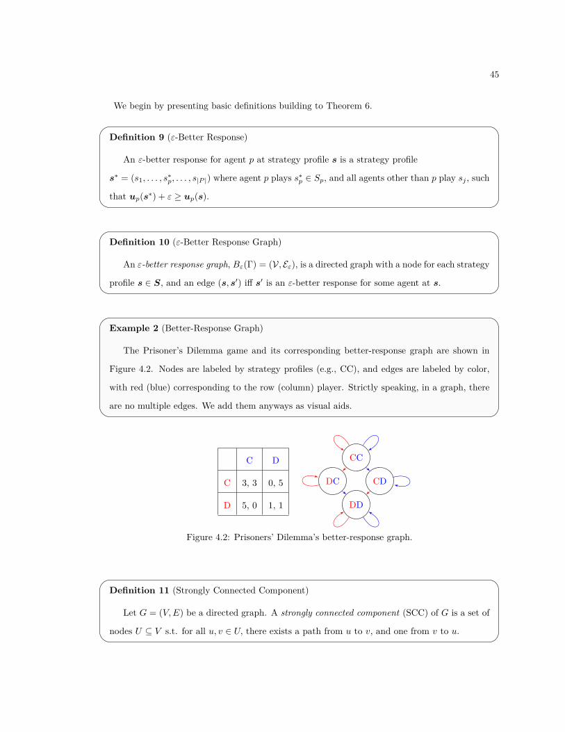
45

We begin by presenting basic definitions building to Theorem 6.

Definition 9 (Á-Better Response)

An Á-better response for agent p at strategy profile s is a strategy profile

sú = (s1, . . . , súp, . . . , s|P |) where agent p plays s

úp œ Sp, and all agents other than p play sj , such

that up(sú) + Á Ø up(s).

Definition 10 (Á-Better Response Graph)

An Á-better response graph, BÁ(�) = (V, EÁ), is a directed graph with a node for each strategy

profile s œ S, and an edge (s, sÕ) i� sÕ is an Á-better response for some agent at s.

Example 2 (Better-Response Graph)

The Prisoner’s Dilemma game and its corresponding better-response graph are shown in

Figure 4.2. Nodes are labeled by strategy profiles (e.g., CC), and edges are labeled by color,

with red (blue) corresponding to the row (column) player. Strictly speaking, in a graph, there

are no multiple edges. We add them anyways as visual aids.

C D

C 3, 3 0, 5

D 5, 0 1, 1

CC

DC CD

DD

Figure 4.2: Prisoners’ Dilemma’s better-response graph.

Definition 11 (Strongly Connected Component)

Let G = (V, E) be a directed graph. A strongly connected component (SCC) of G is a set of

nodes U ™ V s.t. for all u, v œ U, there exists a path from u to v, and one from v to u.

46

1 + Á, 1 + Á

1 ≠ Á, 1 ≠ Á

1 ≠ Á, 1 ≠ Á

1 ≠ Á, 1 ≠ Á

(a) BRG of game �a with 2 players and 2 strategies

1, 1

1, 1

1, 1

1, 1

(b) BRG of game �b with 2 players and 2 strategies

Figure 4.3: An example showing that sink equilibria are inapproximable. To avoid clutter, we donot draw self-loops in the best-response graphs.

Example 3 (Inapproximability of sink equilibria)

Recall that a game’s sink equilibrium is a strongly connected component of its corresponding

better-response graph with no outgoing edges, i.e., edges that connect to other components.

Figure 4.3 shows two games, �a and �b. Game �a (subfigure (a)) is compatible with game �b

(subfigure (b)), and they are uniform approximations of each other, i.e., Î�a ≠ �bÎŒ Æ Á. Note

that �a has two sink equilibria: one consisting of the top-left profile and another consisting of

the remaining three profiles. The entire BRG of �b is the unique sink equilibrium of �b.

It is not hard to see that this example can extend arbitrarily so that the top-left strategy

profile of �a remains its unique sink equilibrium. Coupled with a game analogous to �b where

all utilities but those in top-left are 1≠Á, we see that a sink equilibrium can degrade arbitrarily.

More precisely, we see that, even if a game is close to another, the sink equilibria given by some

approximation can contain an arbitrary number of profiles not in the original sink.

In example 3, we see that the requirement of having no outgoing edges can be easily lost in an

approximated game, even if the approximation is very close. In fact, the example shows that this

is the case for any Á > 0. Instead, we next consider Á-SCC equilibrium as a weaker notion of sink

equilibria that lifts the requirements of components having no outgoing edges. Formally, an Á-SCC

equilibrium is a SCC of an Á-better response graph. We denote by SCCÁ(�) the set of all Á-SCC

equilibria of �. Similarly, an Á-sink equilibrium is a SCC of an Á-better response graph.

47

Theorem 6 (Approximate Equilibria). Let Á > 0. If �Õ is a uniform Á-approximation of �, then

SCC0(�) SCC2Á(�Õ) SCC4Á(�), where A B means that for all A œ A, there exist B œ B,

such that A ™ B.

The keen reader might find similarities between Theorem 6 (approximation guarantees for SCC)

and Theorem 1 (approximation guarantees for Nash equilibria). We show Theorem 6 via a lemma

concerning the edge set of the better-responses graphs of uniform approximations.

Lemma 2 (Á-BRG edges containment.). Let Á > 0. If �Õ is a uniform approximation of �, then

E0(�) ™ E2Á(�Õ) ™ E4Á(�).

Proof. If (s, t) œ E0(�), then there exists p such that up(t) Ø up(s). The following chain of reasoning

then holds: uÕp(t) + Á Ø up(t) Ø up(s) Ø uÕ

p(s) ≠ Á, where the first and last inequalities follow from

the uniform approximation assumption. Hence, uÕp(t) Ø uÕ

p(s) ≠ 2Á, and thus (s, t) œ E2Á(�).

Now, starting from the assumption that (s, t) œ E2Á(�), the following chain of reasoning also holds:

up(t) + Á Ø uÕp(t) Ø uÕ

p(s) ≠ 2Á Ø (up(s) ≠ Á) ≠ 2Á = up(s) ≠ 3Á. Hence, up(t) Ø up(s) ≠ 4Á, and

thus (s, t) œ E4Á(�).

Proof of Theorem 6. We now show that Theorem 6 follows from Lemma 2. We must show that any

SCC of B0(�) remains strongly connected in B2Á(�Õ). Consider Z œ B0(�). Since all the edges in

E0(�) are also present in E2Á(�Õ), it follows that any path connecting two nodes in Z is preserved

in E2Á(�Õ). Consequently, Z remains strongly connected in B2Á(�Õ). Similarly, any SCC of B2Á(�Õ)

remains strongly connected in B4Á(�).

Having shown that SCCs are statistically tractable, we now tackle the problem of optimizing

the designer’s objective function when viewed as a black-box optimization problem. The designer

function maps a strategy profile to a number that measures the designer’s satisfaction if the game

reaches said strategy profile at equilibrium. In the next section, we set aside equilibria estimation

and focus on optimizing the designer’s function for noisy measurements. Later, in section 4.4, we

present our final EMD methodology, which combines both our EGTA methodology, using SCC as

our solution concept, with the methods of the next section to find near-optimal mechanisms.

48

Figure 4.4: The Gaussian approximation of a 90% confidence interval on [0.1, 0.6] where F rangesover [0, 1].

4.3 Black-Box Optimization with Noisy Measurements

In this section, we define two generic black-box optimization problems, and two corresponding

algorithmic solutions. The first algorithm is primarily of theoretical interest; the second is heuristic,

but more practical. Later, using the fact that empirical mechanism design is an instance of black-box

optimization, we apply our heuristic approach to two EMD applications.

Definition 12 (Optimization with noisy measurements (OwNM))

Given a design space �, an objective function F : � æ R, a noise model D , and a measure-

ment operator M : � æ PF , where PF is the space of all possible probability distributions over

the range of F , find ◊ú

œ arg max◊œ� F (◊).

We are concerned with a specific form of measurements, which produce piecewise constant uni-

form noise. This noise model is that which results from probably approximately correct (PAC)-style

guarantees of the form, “accuracy is achieved up to additive error Á with probability 1 ≠ ”” [123].

More formally, we assume the measurement operator M returns F (◊) along with an additive

error bound Á that holds with probability 1 ≠ ”. In other words, the algorithm outputs a 1 ≠ ”

confidence interval [c1, c2] of width 2Á centered at F (◊). Now assuming the range of F (◊) is [c≠, c+],

and letting � .= c+ ≠ c≠, we take as a sample measurement of the pdf pF (x) the following:

49

pF (x) =

Y__________]

__________[

”�≠2Á c≠ Æ x < c1

1≠”2Á c1 Æ x Æ c2

”�≠2Á c2 < x Æ c+

0 otherwise

, (4.1)

Figure 4.4 depicts an example of such a distribution. Intuitively, this distribution captures our

complete ignorance about the value of the objective function, except that it lies somewhere in the

interval [c1, c2] with probability 1 ≠ ”, and elsewhere with probability ”. This model is only valid if

both lower and upper bounds of the objective function are known and finite, but we use this same

information to achieve our PAC guarantees anyway.

Algorithm 3 PAC-OwNM1: procedure PAC-OwNM(�, F, D , Á, ”, �) æ (◊ú

, F (◊ú))2: input:

finite design space �designer’s parameterized black-box objective function F

distribution D

error tolerance Á


range �

3: output:

maximizing parameter ◊ú

designer’s approximate black-box objective value F (◊ú).

4: m Ω

Ï(�/Á)2 ln(2|�|/”)/2

ÌÛ Hoe�ding bound

5: X Ω DmÛ Draw m samples from D

6: for ◊ œ � do7: F [◊] Ω Measure(◊, F, X)8: end for9: ◊

úΩ arg max◊œ� F [◊]

10: return (◊ú, F [◊ú])

11: end procedure

50

4.3.1 Exhaustive Search

In the special case where the parameter space is finite and is searched exhaustively, it is straightfor-

ward to extend PAC guarantees on multiple independent measurements to a global guarantee across

the search space. Algorithm 3 presents such an exhaustive search, and Theorem 7, which again

invokes Hoe�ding’s inequality, describes the guarantee it achieves.

Consider a design space � and an objective function F : � ‘æ [c≠, c+], with � .= c+ ≠ c≠. Let

F1(◊), . . . , Fm(◊) be a sequence of m i.i.d. samples of F (◊) drawn from distribution D .

Hoe�ding’s inequality [62] upper bounds the probability that the absolute di�erence between the

empirical mean and its expected value exceeds Á as

PrX≥D

Q

a

------ED

[F (◊)] ≠1m

mÿ

j=1Fj(◊)

------Ø Á

R

b Æ 2e≠2Á2m/�2

Theorem 7 (PAC-Exhaustive). Consider an OwNM problem s.t. ◊ú

œ arg max◊œ� F (◊), and as-

sume the measurement noise is uniform piecewise constant. Algorithm 3 applied to such a problem

outputs parameter ◊ú and value F [◊ú] such that

---F (◊ú) ≠ F [◊ú]--- Æ Á with probability at least 1 ≠ ”,

where ” =q

◊œ� 2e≠2Á2m/�2 .

Proof. Algorithm 3 explores the entire parameter space. By applying a union bound to Hoe�ding’s

inequality, it follows that all confidence intervals (CI) hold simultaneously, with probability 1 ≠ ”.

The algorithm then returns the maximum measurement, namely F [◊ú]. We can bound the

di�erence between this output and the optimal value F (◊)ú as follows:

≠Á Æ F (◊ú) ≠ (F (◊ú) + Á) Æ F (◊ú) ≠ F [◊ú] Æ (F [◊ú] + Á) ≠ F [◊ú] Æ Á

On the left, we used the CI around F [◊ú] and the fact that F (◊ú) is optimal; on the right, we used

the CI around F [◊ú] and the fact that F [◊ú] Ø F [◊ú]. Therefore,---F (◊ú) ≠ F [◊ú]

--- Æ Á.

To summarize, given Á, ”, and �, Algorithm 3 calculates the requisite number of samples m to

ensure that the output is accurate up to additive error Á with probability 1 ≠ ”.

51

4.3.2 Heuristic Search

Algorithm 3 exhaustively searches the whole design space. But this is impossible for uncountable and

continuous spaces, and becomes computationally prohibitive very fast even for countable, discrete

finite spaces. Hence, we seek a methodology that can find a good approximation of ◊ú using limited

computational resources. That is the search problem we address presently. The problem can be

stated in general terms as follows:

Definition 13 (Budget-constrained optimization with noisy measurements (BCOwNM))

Given a design space �, an objective function F : � æ R, a noise model D , and a measure-

ment operator M : � æ PF , where PF is the space of all possible probability distributions over

the range of F , approximate

◊ú

œ arg max◊œ�

F (◊)

as well as possible, invoking M no more than some budget B œ N times.

Bayesian optimization (BO) is a common tool used to solve BCOwNM problems. BO works by

constructing and maintaining a probabilistic model of the objective function. After sampling, the

probabilistic model is updated accordingly. This model is used to decide where to take the next

measurement, until the budget is exhausted.

Most implementations of BO employ a Gaussian Process (GP) to model the uncertainty sur-

rounding the objective function. Technically, a GP is a collection of random variables, any finite

number of which are jointly distributed by a Gaussian [103]. BO with a GP model has been shown to

outperform state-of-the-art global optimization methods in a number of benchmark problems (e.g.,

[118]).

Standard GPs can handle measurements with i.i.d. Gaussian noise by adding a diagonal term to

the covariance matrix [103]. But there is no easy way to incorporate general noise models into GPs.

We incorporate piecewise constant uniform noise into a GP, heuristically, using the Gaussian that

best approximates pF (x), by minimizing the Kullback-Leibler divergence, DKL.

52

Definition 14 (Best Approximating Gaussian)

Given a continuous (discrete) random variable x with pdf (pmf) p, the best approximating

Gaussian qú is one s.t.

qú(x) œ arg min

q(x)DKL [p(x), q(x)]

The following proposition is straightforward.

Proposition 1. Given any distribution pF (x) in the form of Equation 4.1, the best approximating

Gaussian has mean µú = c1 and variance ‡

ú = 0 when c1 = c2, otherwise they are given by:

µú = –

2!c

21 + c

2+ ≠ c

2≠ ≠ c

22"

+ —

2!c

22 ≠ c

21"

‡ú =

Ú–

2!c

31 + c

3+ ≠ c

3≠ ≠ c

23"

+ —

3 (c32 ≠ c

31) ≠ µú2

where –.= ”

�≠2Á and —.= 1≠”

2Á . It is easy to show that µú and ‡

ú are precisely the mean and variance

of pF (x).

For any valid confidence interval (i.e., one that lies completely within the range of the function

F ), the square root operand is necessarily positive, which means that a real-valued solution always

exists. The singular case where Á = 0 (i.e., c1 = c2) occurs only if c1 = c+ or c2 = c≠.

There are (at least) two ways to utilize Proposition 1 within BO. The first is to assume Gaussian

noise with mean µú and variance ‡

ú, i.e., take µú as the measured value and ‡

ú as the noise in

the measurement process. This is the best possible white noise approximation. We refer to this

approach as GP-N .

One shortcoming of GP-N is that repeated measurements at the same value of ◊ are likely to

produce very similar confidence intervals that do not significantly improve the accuracy of the prob-

abilistic model. Nonetheless, we consider GP-N as a baseline. As an alternative heuristic approach,

we assume Gaussian noise with mean µú and variance 0, thereby avoiding repeated measurements.

We refer to this approach as GP-M.

GP-M may seem incorrect as compared to GP-N , but the width of the confidence interval, 2Á,

is independent of ◊ and known, given the mean of the GP, so it is possible to recover the correct

posterior at any point by adding to the posterior at that point a diagonal matrix that encodes the

disregarded variance. But as we use the GP only to guide the search, this correction is not required.

53

The main advantage of GP-M over the more straightforward GP-N approach is improved ex-

ploration. As a second heuristic approach in this same spirit, we consider a third variant, which

we call GP, in which the variance is again zero, but the mean is set to the mean of the confidence

interval, namely F (◊). This approach, while simple and intuitive, is not the best possible Gaussian

approximation, since µú need not equal F (◊).

4.4 EMD: Putting it all together

Next, we describe how EMD can be viewed as an instance of black-box optimization. We then

proceed to apply the aforementioned BO heuristics to two EMD applications.

Let � be an abstract design space over which a mechanism designer is free to choose parameters

◊ œ �. Conditioned on ◊, we denote by �◊ the ensuing ◊-parameterized game where, in the definition

of a normal-form game (def. 1), we augment all strategies and utilities to depend on ◊. We define

�◊.= ÈP, S◊, u◊(·)Í, where S◊ and u◊(·) denote the dependency of strategies and utilities on ◊.

Overloading notation, we write f(s(◊); �◊) to denote the value of the designer’s objective in

game �◊ at strategy profile s(◊). In optimizing f , the designer assumes that players will play at (or

near) equilibrium. So, as ◊ varies, the value of f likewise varies, as s(◊) potentially moves from one

equilibrium to another.

While solution concepts are meant to be predictive—that is, to predict the outcome of a game—

most yield sets of equilibria, rather than unique predictions. Accordingly, a mechanism designer

often faces a choice. In this work, we assume they choose a worst-case outcome, minimizing the

value of f over the set E(�◊) of equilibria of �◊. We denote this worst-case objective by FE(◊; �◊) =

minsœE(�◊) f(s; �◊). More generally, for Á Ø 0, letting EÁ(�◊) denote the set of equilibria of �◊ up to

Á, we define FEÁ (◊; �◊) = minZœEÁ(�◊) minsœZ f(s; �◊). (N.B. We usually write s œ S◊, suppressing

the dependency of strategies on ◊, because strategies always depend on ◊, and ◊ is usually clear from

context.)

The worst-case EMD problem is to optimize the black-box, worst-case objective function FE(◊; �◊).

Our approach to this problem is to learn the designer’s objective f up to some additive error Á, and

then optimize the corresponding objective FEÁ (◊; �◊). We now argue that this approach is reasonable,

assuming SCCs as the equilibria.

54

Definition 15 ((◊, Á)-approximable objective function)

Let �◊ and �Õ◊ be two ◊-parameterized games, and let f be a designer’s objective. If

max◊œ�,sœS◊ |f(s; �◊) ≠ f(s; �Õ◊)| Æ Á, then we say that the objective f is Á-approximable.

The next theorem states that, for Á > 0, when f is Á-approximable, a solution to the Á-worst-case

EMD problem is an Á-approximate solution to the exact problem, assuming SCC as the equilibrium.

Theorem 8. Let ◊ú optimize F

SCC(◊; �◊), and let ◊úÁ optimize F

SCC

Á (◊; �◊), for Á > 0. If f is

Á-approximable, then--F SCC(◊ú; �◊) ≠ F

SCC

Á (◊úÁ ; �◊)

-- Æ Á.

We show Theorem 8 via an intermediate lemma, which shows that when f is Á-approximable,

FEÁ (◊; �) well approximates F

E(◊; �), assuming E = SCC: i.e.,

FE(�) .= F

SCC(◊; �) = minZœE(◊;�)

minsœZ

f(s; �)

Lemma 3. If f is Á-approximable, then for all ◊ œ �,--F SCC(◊; �◊) ≠ F

SCC

Á (◊; �Õ◊)

-- Æ Á.

Proof. First, note that the strongly connected components of a graph partition its vertices. There-

fore, for all Á Ø 0, it holds that,

FSCCÁ (◊; �◊) = min

ZœSCCÁ(�◊)minsœZ

f(s; �◊) = minsœS◊

f(s; �◊)

Now,F

SCC(◊; �◊) ≠ FSCCÁ (◊; �Õ

◊) = minsœS◊

f(s; �◊) ≠ minsœS◊

f(s; �Õ◊)

Æ minsœS◊

f(s; �◊) ≠ minsœS◊

(f(s; �◊) ≠ Á)

= Á.

A similar argument shows that FSCC(◊; �◊) ≠ F

SCCÁ (◊; �Õ

◊) Ø ≠Á, which completes the proof.

(Proof of Theorem 8). First, observe the following: FSCC(◊ú; �◊) Ø F

SCC(◊Õ; �◊) Ø FSCCÁ (◊Õ; �Õ

◊)≠Á.

The first inequality follows from the fact that ◊ú maximizes F , and the second, from Lemma 3. Via

analogous reasoning, FSCCÁ (◊Õ; �Õ

◊) Ø FSCCÁ (◊ú; �Õ

◊) Ø FSCC(◊ú; �◊)≠Á, assuming ◊

Õ maximizes FSCCÁ .

Together, these two inequalities imply the result.

55

Note that Theorem 8 also holds for the best-case EMD problem, assuming SCC as the equilib-

rium, which is to optimize FSCC = max

ZœSCCÁ(�◊)maxsœZ

f(s; �◊).

Algorithm 4 EMD_Measure1: procedure EMD_Measure(�◊, f, X) æ F (◊)2: input:

parameterized simulation-based game �◊

designer’s objective function f

m samples X

3: output:

Designer’s approximate black-box, worst-case objective value F (◊)

4: for p œ P and s œ S◊ do5: up(s) Ω

1m

qmj=1 up(xj , s)

6: end for7: �◊ Ω ÈP, S◊, u(·)Í Û Empirical parameterized game8: SCCÁ(�◊) Ω FindSCCs(�◊, Á) Û Find SCCs of empirical game9: F (◊) Ω min

ZœSCCÁ(�◊)minsœZ

f(s; �◊)

10: return F (◊)11: end procedure

In sum, it su�ces to approximate f up to Á to obtain an Á-approximation of FSCC(◊; �). Further-

more, it su�ces to optimize FSCCÁ (◊; �◊) up to Á to obtain an Á-approximate solution to the worst-case

EMD problem. Such estimates can be computed with high probability via Algorithm 3, using the

measurement procedure defined in Algorithm 4. But to obtain the usual guarantees, the number

of samples m calculated in Line 4 of Algorithm 3 must be updated toÏ

(�/Á)2 ln(2(|�|+|�|)/”)/2Ì

to

account for a union bound over both the mechanism’s and the game’s parameters.

4.5 Experiments

In this section, we present experimental results using our equilibrium estimation and BO search

methodology. We note that all BO algorithms use a Mattern Kernel [103] in the underlying Gaussian

Process and the expected improvement [118] acquisition function. We use GP-N , GP, and uniform

sampling over the range [0.5, 1.5]8 as our baselines. Note that uniform sampling is a competitive

search strategy for hyper-parameter optimization [20].

56

0 5 10 15 20# of reserve prices searched

0.34

0.36

0.38

0.40

0.42

Run

ning

max

.re

venu

e

� = 0.02

algo

random

gp

gpm

gpn


� = 0.01

algo

random

gp

gpm

gpn

Figure 4.5: FPA search for optimal reserve price, ” = 0.1

We experiment with our methodology in two settings. The first is in first-price auctions where

analytical solutions are known, and the condition of Definition 15 holds, as the revenue curve is a

known to be a continuous function of the reserve price. The second is in a setting with no known

analytical solutions, and with no guarantees as to whether condition of Definition 15 holds or not.

Nonetheless, we report anecdotally that an empirical analog of the condition is often met in our

experiments.

4.5.1 First-price Auctions

As our first application domain, we consider first-price auctions in the standard independent, private

value model [73]. There is one good up for auction, and n bidders, with bidders’ values drawn from

some joint distribution G. Bidders submit bids b1, . . . , bn, and the highest bidder wins and pays

his bid. As a proof of concept, we apply our BO search heuristics in this domain, in attempt to

maximize revenue as a function of a reserve price, r, below which the good will not be sold.

In this controlled setting, analytical solutions are known in certain special cases. For example,

when bidders’ valuations are drawn i.i.d. uniformly on [0, 1], the (unique) symmetric Bayes-Nash

strategy [73] is given by:

s(v) .= (v Ø r) [rn/vn≠1 + (n≠1)(vn≠rn)/nvn≠1]

57

Assuming n = 2 bidders play this equilibrium, the optimal reserve price is 1/2, which yields a revenue

of 5/12.

Figure 4.5 depicts a comparison of GP-M and GP against the baselines, GP-N and uniform

sampling, for Á œ {0.02, 0.01}. We note that a similar behavior was observed for Á = 0.03. Specifi-

cally, we plot a running maximum of revenue as a function of the number of reserve prices searched.

Each point is an average over 30 trials, where a single trial consists of exploring 20 di�erent reserve

prices with di�erent initial random points. All the BO heuristics are initialized with the same three

initial random points.

Our BO heuristic GP-M consistently outperforms uniform sampling and GP-N (whose predicted

anomalous behavior was explained in Section 4.3), taking fewer measurements to achieve near-

optimal values of revenue. The close performance between GP-M and GP can be explained by the

fact that ” is so small that the mean of a measurement’s confidence interval is close to µú.

4.5.2 Advertisement Exchange

In this section, we illustrate our EMD methodology in a one-shot advertisement exchange game,6

a game rich enough that analytic solutions are not readily available, but nonetheless amenable to

probabilistic analysis through sampling and simulation. The game is designed to model a scenario

common in electronic advertisement platforms, such as Google’s AdWords© and Amazon Sponsored

Brands©.

We begin by describing, at a high-level,7 the elements and dynamics of the game, and the

strategies used by agents. We conclude with experiments showing that our algorithms more quickly

accrue higher revenue than a baseline in an 8-dimensional parameter space.

AdX game in a nutshell.

In the AdX game, agents play the role of advertising networks competing in an exchange for op-

portunities to show Internet users impressions (i.e., advertisements) needed to fulfill advertising

campaigns. These impression opportunities (henceforth, impressions) are sold in real-time sequen-

tial auctions, as users arrive, but agents submit their bids in advance, placing potentially di�erent

bids for di�erent classes of users.6A simplification of TAC AdX [116].

7A complete mathematical formalization of this game is given in chapter 5.

58

Users are characterized by attributes: e.g. Gender, Income, Age, etc., each of which is char-

acterized by a set of attribute values: e.g., {Young, Old}. Each user belongs to a market segment,

which is a list of values for (not necessarily all) attributes: e.g., ÈFemale, YoungÍ.

A market segment M matches another market segment MÕ if all the attribute values in MÕ are

present in M. For example, the market segments ÈFemale, Young, High IncomeÍ and ÈFemale,

Young, Low IncomeÍ both match ÈFemale, YoungÍ; however, ÈFemaleÍ does not match ÈFemale,

YoungÍ, since attribute value Young is missing from the former.

In the AdX game, agents target (i.e., aim to display advertisements to) some market segments,

but not others, as described by their (single) advertising campaign. Each advertising campaign

Cj = ÈIj ,Mj , RjÍ demands Ij œ N impressions in total, procured from users belonging to any

market segment MÕ that matches the campaign’s desired market segment Mj . A campaign’s budget

Rj œ R+ is the maximum amount the advertiser is willing to spend on those impressions. From the

agent’s point of view, the budget maps to its potential revenue.

To a first approximation then, agent j’s goal, is to procure at least Ij impressions matching

market segment Mj to fulfill Cj ’s so that it can earn revenue, which depends on Rj . (Note that

impressions in market segments other than Mj yield no value.) More specifically, the value of a

number of procured impressions z is determined via a sigmoidal function that maps z to a percentage

of the budget: i.e., small values of z yield a small percentage of Rj , while values close to Ij yield

values close to Rj . The non-linearity inherent in this function models complementarities, 8 because

it incentivizes agents to focus either on completely satisfying a campaign’s demand, or not to bother

satisfying it at all.

The AdX game is a one-shot game. To play, agents submit bids and spending limits for each

market segment. Then, simulated users arrive at random, from the various market segments. For

each user that arrives from market segment M, a second-price auction with a publicly known reserve

price rM œ R+ is held among all agents whose bids match M, and who have not yet reached their

spending limit in M. Agent j’s utility is computed as the di�erence between its revenue and its

expenditure for all auctions.8A good is a complement of another if the value of acquiring both is strictly greater than the value of acquiring

either one of them but not the other: e.g., the value of acquiring a pair of shoes (left and right) is usually greater

than the value of only the left or the right one.

59

Strategies.

Designing bidding strategies for electronic ad exchanges (and ad auctions, more generally) is an

active research area (e.g. [30, 43, 50]). The goal of these experiments is not to investigate the

performance of state-of-the art bidding strategies, though this is certainly an interesting future

research direction, but rather to test the methodology developed in this thesis. Toward this end, we

devised two heuristics which, we call Walrasian Equilibrium (WE) and Waterfall (WF). Detailed

descriptions of these heuristics are provided in chapter 5. Here, we present only their main ideas.

At a high level, both heuristics work by building an o�-line model of the market induced by the

AdX game, which is then used to compute an allocation (assignment of impressions to campaigns)

and prices (for impressions), based on which bids and limits are determined. The strategies di�er

in how this outcome—the allocation and prices—are computed. In a nutshell, the WE strategy

searches for an outcome which forms a near-Walrasian equilibrium, i.e., an outcome whose prices

provide little incentive for agents to relinquish their allocation. The study of equilibria and near-

equilibrium computation in combinatorial markets (ad exchanges, being one example) is an active

research area (e.g., [25, 44, 48]) with promising applications (e.g., [4, 79, 82]). The WF strategy works

by simulating the arrival of impression opportunities in a fixed order that is endogenously determined

by the campaigns present in the market. We call this strategy Waterfall because impressions are

allocated to campaigns in descending order of budget-per-impression, and from market segments

in ascending order of second-highest budget-per-impression. Hence, the final bid prices can be

visualized as a descending waterfall-like structure.

4.5.3 Experimental Setup

We assumed three user attributes: gender, age, and income level, each with two values. We then

simulated a fixed number of impression opportunities, namely K = 500, distributed over 8 market

segments, corresponding to all the possible combinations of attribute values: {Male, Female} ◊

{Young, Old} ◊ {Low Income, High Income}. The distribution fi over these impression oppor-

tunities was constructed from statistical data at www.alexa.com [116].

Each agent’s campaign Cj = ÈIj ,Mj , RjÍ is determined as follows: A market segment Mj is drawn

uniformly over all 20 possible market segments corresponding to combinations of user attributes of

size 2 (e.g., ÈMale, YoungÍ) and 3 (e.g., ÈMale, Young, Low IncomeÍ). Given Mj , the demand

www.alexa.com

60

Ij := KfiMj/N, where KfiMj is the expected size of market segment Mj , and N is the number of

agents in the game. Given Ij , the budget Rj is a noisy signal of the demand modeled by a beta

distribution: Rj ≥ Ij(B(– = 10, — = 10) + 0.5).

The task is to find an 8-dimensional vector of reserve prices r œ R8, consisting of one reserve

price per market segment, that maximizes the auctioneer’s revenue, up to a desired accuracy Á and

specified failure probability ”. We experiment with N = 4 agents, and two possible strategies; in

particular, for all p, Sp = {WE, WF}. Since by construction these strategies never bid higher than a

campaign’s budget-per-impression, Rj/Ij = B(– = 10, — = 10) + 0.5 œ [0.5, 1.5], we bound the search

for each reserve price to this same range, and hence search the space [0.5, 1.5]8.

Even in this bounded region, the complexity of this task is substantial: for each candidate vector

of reserve prices, we must first learn the corresponding game it induces, and then solve for the

equilibria of this game. In this thesis, we use Algorithm 4 for this purpose, which finds the set SCCÁ

using Tarjan’s algorithm [119], and then returns the minimum revenue among all SCCÁ equilibria.

This is a computationally intensive task. Indeed, it took approximately 5 days to obtain these

results using 4 machines, each with an E5-2690v4 (2.60GHz, 28Core) Xeon processor, and 1,536 GB

of memory.


0.23

0.25

0.28

0.30

0.33

0.35

0.38

0.40

Run

ning

max

.re

venu

e

� = 0.03

algo

random

gp

gpm

gpn


� = 0.02

algo

random

gp

gpm

gpn

Figure 4.6: AdX search for optimal reserve prices, ” = 0.1

61

Algorithm 5 Experimental Procedure1: procedure ExperimentalProcedure(�r, f, X, nt, ni, ns) æ {µs}

nss=1

2: input:

simulation-based game parameterized by reserve prices �r

designer’s objective function f

samples X

number of trials nt

number of initial reserves ni

number of search steps ns

3: output:

running maximum, {µs}nss=1, for ns search steps, averaged across nt trials.

4: for t = 1, . . . , nt do Û nt trials.5: � = {r1, . . . , rni} Ω GetInitialReservePrices(t) Û Get ni initial reserve price vectors.6: N.B. rj =

+r1

j , . . . , r8j

,œ R, where rM

j is the reserve price in market segment M.7: for r œ R do8: Ft(r) Ω EMD_Measure(�r, Revenue, X) Û Call to Algorithm 49: end for

10: Gt Ω InitializeGaussianProcess({r, Ft(r)}rœR)11: ‹t = [] Û Store trial t’s running maximum in a list12: for s = 1, . . . , ns do Û ns search steps.13: rt

s Ω AcquisitionFunction(Gt) Û We use Expected Improvement14: Ft(rt

s) Ω EMD_Measure(�rts, Revenue, X) Û Call to Algorithm 4

15: ‹t[s] = maxkÆs Ft(rtk) Û Compute current running maximum

16: Gt Ω UpdateGaussianProcess(Gt, {rts, Ft(rt

s)})17: end for18: end for19: for s = 1, . . . , ns do20: µs Ω 1

nt

qnt

t=1 ‹t[s] Û Averaging across trials21: end for22: return {µs}ns

s=1

23: end procedure

4.5.4 Experimental Results

Experimental results in Figure 4.6 were obtained by running the procedure described in Algorithm 5,

for each of GP, GP-M, and GP-N . This procedure takes as input a simulator for parameterized

game �◊, a designer’s objective function f (in this case, revenue), samples X, a number of trials nt,

a number of initial reserve prices ni, and a number of search steps ns. It then outputs a sequence

of length ns, {µs}nss=1, where each µs is the running maximum of the revenue obtained by to step

s, averaged across nt independent trials. More specifically, letting t index trials and s index steps,

62

µs = 1nt

qnt

t=1 maxkÆs Ft(rtk), where Ft(rt

k) is the revenue assuming reserve prices rtk, which denotes

the reserve prices explored during the kth step of the tth trial.

Figure 4.6 summarizes our AdX results. Specifically, we plot a running maximum of revenue

as a function of the number reserve prices evaluated so far. Each plot is an average over 30 trials,

where a single trial consists of exploring 100 di�erent vectors of reserve prices, initialized at random.

To ensure a fair comparison, all search algorithms are fed the same 10 initial points during each

trial. These results are compared to uniform sampling. As in the first-price auction experiment,

our BO heuristic GP-M outperforms uniform sampling and GP-N , taking fewer measurements to

achieve higher values of revenue. GP-M’s performance is on par with that of GP, which once

again can be explained by a su�ciently small value of ”. Note, however, the apparent di�culty in

optimizing revenue in this game; GP-M and GP take significantly more measurements to outperform

the baselines. Nonetheless, these results show that, even under a fairly constrained budget, our BO

heuristics are e�ective as compared to our baselines.

63

4.6 Chapter Summary

Our EMD methodology tackles the fundamental problem of optimizing a designer’s objective function

in parametric systems inhabited by strategic agents. The fundamental assumptions are: 1) players

play equilibria among an a priori known set of strategies, which in general depend on the parameters

of the system; and 2) there is no analytical description available of either the strategies or the system,

but only a simulator (i.e., a procedural description) capable of producing data about game play. This

framework captures modern, computationally intensive systems, such as electronic advertisement

exchanges. The challenge then is two-fold: first, one must learn equilibria of a game for a fixed

setting of parameters, and second, one must search the space of parameters for those that maximize

the designer’s function.

Our main contribution is a PAC-style framework to solve the former, while for the latter we

enhance standard search routines for black-box optimization problems to include piecewise constant

noise, precisely the kind of noise that characterizes PAC learners. We prove theoretical guarantees

on the quality of the learned parameters when the parameter space is finite. We also demonstrate

the practical feasibility of our methodology, first in a setting with known analytical solutions, and

then in a stylized but rich model of advertisement exchanges with no known analytical solutions—

precisely the kind of setting for which we devised our methodology—and show that we can find

solutions of higher quality than standard baselines.

We emphasize that evaluating the quality of a mechanism produced by our EMD methodology

is itself a challenging task. In addition to developing an ad exchange model, we created two bidding

heuristic strategies that operate in it. Beyond using them in our experimental evaluations in this

chapter, this model and heuristics are intricate and of interest on their own. Thus, we detailed them

in the next chapter.

Chapter 5

Heuristic Bidding for Electronic

Ad Auctions

In this chapter, we present our contributions to the design of heuristic bidding strategies for electronic

advertisement auctions. The contents of this chapter are complementary to the following published

papers: Principled Autonomous Decision Making for Markets [3], and On Approximate Welfare-and

Revenue-Maximizing Equilibria for Size-Interchangeable Bidders [4] (arXiv version [5]).

5.1 Preliminaries

This chapter presents a detailed mathematical description of the one-day electronic advertisement

game (one-day AdX) that we devised and used to evaluate our EMD methodology in section 4.5.2.

We call this simplified game the one-day AdX to remark that our game models a single day (or any

other arbitrary unit of time) of the more challenging TAC AdX game [116]. Still, the challenge faced

by agents (or ad networks) in our one-day AdX game is substantial. Namely, given a campaign, the

challenge for an ad network is to procure enough display ad impression opportunities to fulfill the

campaign at the lowest cost possible in the face of competition from other ad networks. We call this

problem the ad network problem. The one-day AdX game is a simplified version of the TAC AdX

that allows us to focus more clearly on the ad network problem.

64

65

Towards developing bidding heuristics for the ad network problem, we first model the market

induced by ad exchanges as a combinatorial market [12, 16, 31, 81]. In our formulation, we model

impression opportunities as the supply side of the market and ad networks as the demand side. Since

demographics characterize impression opportunities, we model each demographic as a single type of

good for which there are potentially multiple units available to consumers.

Having modeled the ad exchange market, we then turn our attention to designing bidding heuris-

tics for the ad network problem. At a high level, our heuristics first compute a prediction of the

market outcome, which consists of an allocation of impression opportunities to ad networks together

with prices for each impression opportunity. An agent that uses our heuristic bidding strategies

submits bids and budget limits to the ad exchange based on said predictions.

We present two di�erent approaches to compute predictions of market outcomes, (1) a market-

equilibrium-based approach (WE heuristic), and (2) an auction-simulation approach (WF heuristic).

In approach (1), our goal is to compute a (near) competitive equilibrium of the market as defined

classically for markets with divisible goods by French economist Léon Walras [132] and more recently

extended to markets with indivisible goods (known in the literature as combinatorial markets [21]).

In approach (2), we simulate the workings of an ad exchange by computing an allocation and

bids that simulate the second-price auctions used to place an advertisement on the internet1. For

tractability, we assume users arrive grouped by their market segments, but the order of arrival is

endogenous, meaning determined by the algorithm.

5.2 Game Elements

An advertising campaign C = ÈI,M, RÍ demands I œ N impressions in total, procured from users

belonging to any market segment MÕœ M that matches the campaign’s desired market segment

M œ M . (The match function, and market segments, are defined precisely below.) A campaign’s

budget R œ R+ is the maximum amount the advertiser is willing to spend on those impressions.

The one-shot AdX game is played by a set A of agents, where each j œ A is endowed with a

campaign Cj = ÈIj ,Mj , RjÍ.

The AdX game is a game of incomplete information. In general, agents do not know one another’s

campaigns. Consequently, agent j’s strategy set consists of all functions mapping agent j’s campaign1For example, Google’s

®AdSense https://www.google.com/adsense/.

https://www.google.com/adsense/

66

Cj (i.e., its private information) to tuples of the form+bj

, lj,. The first component of this tuple

is a bid vector bj =e

bj1, b

j2, · · · , b

j|M |

f, where b

jM œ R+ is agent j’s bid for impressions that match

market segment M. The second component is a limit vector lj =e

lj1, l

j2, · · · , l

j|M |

f, where l

jM œ R+

is agent j’s spending limit on impressions that match M.

Example 4 (A two-player, one-shot AdX game)

The following is an example of a two-player (A = {1, 2}), one-shot AdX game. Let M =

{M1,M2,M3} be a set of three market segments. The first agent’s campaign is defined as

C1 = È10,M1, 100Í. In other words, given a budget of $100, the first agent’s goal is to procure

at least ten di�erent impression opportunities, i.e., ten opportunities to show advertisements to

users. Crucially, each advertisement must be shown to a user that matches market segment M1.

The second agent’s campaign is defined as C2 = È5,M3, 25Í. Likewise, agent 2 has a budget

of $25, and its goal is to show advertisement impressions to at least five users, each of which

matches market segment M3.

Agent’s j œ A = {1, 2} strategy in this game is a function, Cj ‘æ

eeb

j1, b

j2, b

j3

f,

elj1, l

j2, l

j3

ff,

from its campaign to bids and limits. For example, suppose that agent 1 wishes to bid, for each

impression it demands, an amount proportional to its budget. Suppose also that the agent is

only interested in procuring impressions that match M1 (for simplicity, suppose in this example

that Mk matches only with itself for k = 1, 2, 3). Additionally, the agent is unwilling to spend

any amount above its budget for impressions that match its market segment. For impressions

that do not match its market segment, the agent is unwilling to spend any positive amount of

its budget. The agent can realize this strategy with the following mapping,È10,M1, 100Í ‘æ ÈÈ$100/10, 0, 0Í , È$100, 0, 0ÍÍ

Note that the following mapping implements the same kind of strategy for agent 2,È5,M3, 25Í ‘æ ÈÈ0, 0, $25/5Í , È0, 0, $25ÍÍ

We now proceed to define utilities. We start by more precisely defining what it means for a user’s

impression to match an advertiser’s campaign. Let A = {A1, . . . , Ak} be a set of k attributes. Each

attribute is defined as a discrete set of attribute values. A market segment M is defined as a vector

of attribute values, M = Èa1, . . . , akÍ, where ai œ Ai.

67

Example 5 (Attributes, attribute values, and market segments)

Consider the following set of attributes A = {Gender, Income, Age}.

Define, for each attribute, values as follows,

Gender = {Male, Female}, Income = {High, Low}, and Age = {Old, Young}.

In this case, there are 23 = 8 possible market segments, namely, M =

{ÈMale, High, OldÍ , ÈMale, High, YoungÍ , ÈMale, Low, OldÍ , ÈMale, Low, YoungÍ ,

ÈFemale, High, OldÍ , ÈFemale, High, YoungÍ , ÈFemale, Low, OldÍ , ÈFemale, Low, YoungÍ}

We augment each attribute Ai with a special symbol ú to create the augmented attribute Aúi =

Ai fi {ú}. An augmented market segment Mú is a vector of augmented attributes’ values, Mú =

Èaú1, . . . , a

úkÍ, where a

úi œ A

úi . We denote by M the set of all possible augmented market segments.

Given two augmented market segments M and MÕ, we say that M matches MÕ, and write M ∞ MÕ,

if and only if for i = 1, . . . , k, if aÕi ”= ú, then a

Õi = ai. In words, M ∞ MÕ if and only if

1. In case the i-th attribute value of MÕ is the special symbol ú, the i-th attribute value of M is

allowed to be any value.

2. In case the i-th attribute value of MÕ is not ú, the i-th attribute value of MÕ is the same as the

i-th attribute value of M.

Example 6 (Matching market segments)

Using attributes as defined in example 5, the following are matches:

1. ÈFemale, High, YoungÍ ∞ È*, *, *Í.

2. ÈFemale, High, YoungÍ ∞ È*, High, YoungÍ and

ÈMale, High, YoungÍ ∞ È*, High, YoungÍ .

3. ÈFemale, Low, YoungÍ ∞ ÈFemale, *, YoungÍ and

ÈFemale, High, YoungÍ ∞ ÈFemale, *, YoungÍ.

The following are not matches:

1. ÈFemale, High, YoungÍ ”∞ ÈMale, *, *Í, since Female ”= Male.

2. ÈMale, High, YoungÍ ”∞ ÈMale, *, OldÍ, since Young ”= Old.

68

The above definitions are intended to be used to describe which users’ impressions match which

advertisers’ campaigns. Users belong to market segments (and thus, augmented market segments),

and campaigns can be specified in the language of augmented market segments,2 so these defi-

nitions are su�cient for matching impressions with campaigns. Hereafter, we drop the qualifier

“augmented,” as we only ever consider augmented markets segments.

Denote by y =+y1, y2, . . . , y|M |

,a bundle of impressions, where yM œ N denotes the number of

impressions from market segment M in bundle y. The utility uj of agent j, as a function of bundle

y, is given by:

uj(y, Cj) = fl(µ(y, Cj), Cj) ≠ p(y) (5.1)

Here p(y) is the total cost of bundle y, and µ(y, Cj) =q

MœM yM {M ∞ Mj} is a filtering function,

which, given a bundle of impressions and a campaign, calculates the number of impressions in the

bundle that match the campaign. Finally,

fl(z, Cj) =3

2Rj

b

4 3arctan

3bz

Ij≠ a

4≠ arctan(a)

4,

where, for any nonzero k œ R, a = b + k and b is the unique solution to the equation

arctan(k) ≠ arctan(≠b)1 + b

= 11 + k2

Following Schain and Mansour [116], we use k = 1, which implies a ¥ ≠3.08577 and b ¥ 4.08577.

Intuitively, fl(z, Cj) maps a number of impressions z to a percentage of Rj in a sigmoidal fashion:

i.e., small values of z yield a small percentage of Rj , while values close to Ij yield values close to

Rj . The non-linearity inherent in this function models complementarities,3 because it incentivizes

agents to focus either on completely satisfying a campaign’s demand, or not to bother satisfying it

at all. Figure 5.1 depicts a sample sigmoidal, for a campaign that demands 200 impressions. Note

that from an agent’s point of view, its campaign’s budget maps to its potential revenue.

This concludes our description of agents’ types (i.e., their private information), their strategies,

and their utilities in the one-shot AdX game.2Augmented market segments are also a natural way to describe users, since not all user attributes are revealed,

in general.3A good is a complement of another if the value of acquiring both is strictly greater than the value of acquiring

either one of them but not the other: e.g., the value of acquiring a pair of shoes (left and right) is usually greater

than the value of only the left or the right one.

69

Figure 5.1: Sigmoidal for a campaign that demands 200 impressions.

5.3 Game Dynamics

As the one-shot AdX game is a one-shot game, bids and spending limits are submitted to the ad

exchange only once. Still, the game unfolds in four stages.

Stage 0: The agents learn their campaigns. In the current experiments (Section 4.5.2), we

assume agents are well versed in their competition, and thus they also learn one another’s campaigns.

As such, we model the agents playing a complete-, rather than an incomplete-, information game.

Stage 1: The ad exchange announces a vector of reserve prices r œ RM+ , i.e., prices above which

agents must bid to participate in the various auctions, where rM œ R+ is a price above which agents

must bid to participate in auctions for impressions belonging to market segment M œ M .

Stage 2: All agents submit their bids and their spending limits for all auctions: i.e., agent j

submits tuple+bj

, lj,. As the name suggests, this limit is the maximum the agent is willing to spend

on impressions that match M. In case there are multiple matches, the minimum among spending

limits is enforced.

Stage 3: Some random number of impressions K ≥ U [Kl, Ku] arrive in a random ordereM

f=

+M1

,M2, . . . ,MK

,, where Mi

≥ fi =+fi1, fi2, . . . , fi|M |

,, and fiM is the probability of M. For each

impression that arrives from market segment M, a second-price auction with reserve price rM œ R+

is held among all agents whose bids are matched by M, and who have not yet reached their spending

limit in M. If an agent submits multiple matching bids, it does not compete against itself; the

70

maximum of its matching bids is entered into the auction.

Stage 4: The output of stage 3 is, for each agent j, a bundle of impressions

yj =e

yj1, y

j2, . . . , y

j|M |

f, which is used to compute agent j’s utility according to Equation (5.1).

The auctioneer’s revenue is defined asq

j p(yj).

5.4 Strategies

We devised two heuristic strategies for the one-day AdX game. The first heuristic is a market

equilibrium-based approach which we call Walrasian Equilibrium (WE). The second is an auction-

simulation approach which we call Waterfall (WF)4. At a high level, both heuristics work by

collapsing the dynamics of the one-day AdX game into a static market model, which is then used to

compute an allocation (assignment of impressions to campaigns) and prices (for impressions), based

on which bids and limits are determined.

5.4.1 Static Market Model

The static market model employed by both heuristics is an augmented bipartite graph M =

ÈM, C, E, N , I, RÍ, with a set of n œ N market segments M ; a set of c œ N campaigns C; a set

of edges E from market segments to campaigns indicating which segments match to which cam-

paigns; supply vector N = ÈN1, . . . , NnÍ, where Ni œ N is the number of available impressions from

market segment i œ M ; demand vector I = ÈI1, . . . , IcÍ, where Ij œ N is the number of impressions

demanded by campaign j œ C; and reward vector R = ÈR1, . . . , RcÍ, where Rj œ R+ is campaign j’s

reward.

Let’s look at an example of this construction.

4Not to be confused with waterfalling, the process by which publishers try to sell remnant inventory; see https:

//clearcode.cc/blog/what-is-waterfalling/.

https://clearcode.cc/blog/what-is-waterfalling/

https://clearcode.cc/blog/what-is-waterfalling/

71

Example 7 (Static market as a bipartite graph)

As in example 4, suppose that there are two campaigns defined as C1 = È10,M1, 100Í and

C2 = È5,M3, 25Í. Further suppose that M = {M1,M2,M3} and that Mk matches only with

itself for k = 1, 2, 3. To fully specified a market M from this input, we still have to define

the number of available impressions for each market segment. Suppose that there are seven

impressions of M1, three of M2, and six of M3. We can now fully specify M.

Concretely, M = ÈM, C, E, N , I, RÍ where

M = {M1,M2,M3}, C = {C1, C2}, E = {{C1,M1}, {C2,M3}},

N = È7, 3, 6Í, I = È10, 5Í, R = È$100, $25Í

Given a market M, our goal is to compute both an allocation of impression opportunities to cam-

paigns and prices that serve as predictions for bidding strategies. We denote by X œ Zn+ ◊ Zc

+

an allocation matrix, where entry xij is the allocation (i.e., number of impressions) from market

segment i assigned to campaign j. We also denote by p œ Rn+ a price vector, with price pi per im-

pression from market segment i. Pair (X, p) is an outcome of market M in the sense that it resolves

the utility that each agent receives in the game. As defined, this outcome is anonymously-priced

because agents face the same price per impression, pi, for market segment i. We also consider the

case of personalized-priced outcomes where agents might face di�erent prices per impression in the

same market segment. Formally, let P œ Rn+ ◊ Rc

+ be a price matrix, with price pij per impression

from market segment i to campaign j. Then, pair (X, P ) is a personalized-priced outcomes.

5.4.2 Walrasian Equilibrium Bidding Strategy

An anonymously-priced5 Walrasian (or competitive) equilibrium (WE or CE) is a class of market

outcomes of particular interest in mathematical economic theory, with a rich history that extends

as far back as Walras’ work. [132]. In a CE, buyers are utility-maximizing (i.e., they maximize their

utilities among all feasible allocations at the posted prices) and the seller maximizes its revenue

(again, over all allocations at the posted prices). A competitive equilibrium serves as an idealized

prediction of a market outcome6, and thus, our motivation to use it as a predictive model for our

WE heuristic.5If there are multiple copies of some homogeneous good, all copies must have the same price.

6Under a number of assumptions whose validity for the AdX market need to be investigated in future work.

72

Unfortunately, an anonymously-priced WE always exist only for a small class of combinatorial

markets [69] and, consequently, there is a rich line of work dedicated to devising CE relaxations that

retain some of their nice properties [28, 44, 60]. In previous work [4], we noted that a WE outcome

is not guaranteed to exist in a static market model of the one-day AdX game. Still, motivated by

the desired to compute outcomes close to competitive equilibria, we proposed a novel relaxation

of CE, which we called limited envy-free pricing [4, 5].7. We further derived a polynomial-time8

heuristic that computes an approximate revenue-maximizing, limited envy-free pricing. A (slight)

modification of that algorithm forms the core of the WE bidding heuristic.

Next, we summarize the WE bidding heuristic we devised for the ad network problem. We defer

a more in-depth treatment of competitive equilibrium theory in combinatorial markets9, and our

contributions from a statistical learning perspective, to the next chapter.

The WE bidding heuristic works as follow. First, we solve for an approximate welfare-maximizing

allocation (Algorithm 6). A welfare-maximizing allocation is an allocation that maximizes the sum

of agents’ values. Fixing the allocation, we solve for a revenue-maximizing limited envy-free pricing,

abbreviated LEFP (Algorithm 7)10. A LEFP relaxes the requirement that all agents maximize their

utilities at the posted prices and instead insists that only agents that received a non-empty bundle

maximize their utilities. The agent then bids the LEFP price of any market segment for which it has

been allocated and places a limit proportional to its total spending in the segment. In summary, an

agent employing the WE bidding heuristic11 runs Algorithms 6 and 7; then, given (Xr, p), it bids

pi in all market segments i for which xij > 0, and places limits xijpi in all market segments i.

We provided justification for the WE heuristic in previous work [4]. Concretely, we showed in

extensive experimentation using real-world web usage data obtained from www.alexa.com that the

above two-step procedure results in market outcomes that are very close to WE. More specifically, in

a setup akin to the one-day AdX game’s static model, we experimentally showed that the constraints

that define WE are violated with small additive errors, on average, over multiple runs.7Our relaxation, in turn, builds on a previously proposed relaxation known as an envy-free pricing [60]. We also note

that after we proposed our relaxation, researchers have further studied it under the name of buyer preselection [23, 24].8Since electronic advertisement markets operate under tight time requirements, computational tractability is of

paramount importance.9In a combinatorial market, goods cannot be divided, but instead, each must be either wholly allocated to a single

consumer or not allocated at all. The one-day AdX static market M is an example of a combinatorial market since

impression opportunities cannot be divided among multiple agents.10

Note that Algorithms 6 and 7 slightly generalize those presented in [4], in that they handle a vector of reserve

prices, one per market segment.

11As currently described, supply vector N remains undefined. In our experiments, we use the expected number of

available impressions for each market segment. This number ignores the order of arrival of impressions and instead

assumes that there are enough of them so that the exact order is not of importance but their total quantity.

www.alexa.com

73

Algorithm 6 Greedy allocation algorithm1: procedure GreedyAllocation(M, r)æ Xr

2: input:

market M

reserve prices r œ Rn+

3: output:

Allocation Xr

4: for all i, j, initialize xij = 05: for j œ C do Û Loop through j in descending order of bang-per-buck, i.e., Rj/Ij.6: Let Ej = {i œ M | {i, j} œ E and

qcj=1 xij < Ni}

7: ifq

iœEjNi ≠

qcj=1 xij Ø Ij then Û “enough supply remains to satisfy j”

8: for i œ Ej do Û Loop through Ej in descending order of supply.9: xij = min{Ij ≠

qni=1 xij , Ni ≠

qcj=1 xij}

10: end for11: if

qni=1 rixij > Rj then Û “campaign j cannot a�ord the assigned bundle”

12: for all i: xij = 0 Û Unallocate j.13: end if14: end if15: end for16: return Xr

17: end procedure

Algorithm 7 Linear program that computes (near) revenue-maximizing LEFP1: procedure LEFP(M, r, Xr)æ p

2: input:

Market M

reserve prices r œ Rn+

allocation Xr

3: output:

A pricing p

4: maximizep,–q

jœC,iœM xijpi ≠q

jœC,(i,k)œM◊M –jik, subject to:5: (1) ’j œ C : If

qni=1 xij > 0, then

qni=1 xijpi Æ Rj

6: (2) ’i œ M, ’j œ C :If xij > 0 then ’k œ M : If {k, j} œ E and xkj < Nk then pi Æ pk + –jik

7: (3) ’i œ M : pi Ø ri

8: (4) ’j œ C, ’(i, k) œ M ◊ M : –jik Ø 09: return p

10: end procedure

74

5.4.3 Waterfall Bidding Strategy

The Waterfall heuristic (WF) is designed to simulate the dynamics of the one-shot AdX game. In the

game, the highest bid in a market segment stands for some period of time, namely until the spending

limit of the winning campaign is reached, or the campaign is satisfied. Hence, prices in each market

segment remain constant for some period of time at the current highest bid. As the game unfolds,

more and more impressions are allocated, consuming the budgets of the winning campaigns in each

market segment, until the winners drop out, and the second highest bidder is promoted. The bid of

the campaign that drops out is by definition higher than the new winning bid, which again stands

for some further period of time. The resulting prices thus resemble a waterfall: i.e., decreasing, and

constant between decreases.

An agent employing the WF heuristic computes an allocation X and a price matrix P via

Algorithm 8, given a market M and reserve prices r. The algorithm works by simulating n second-

price auctions assuming agents bid Rj/Ij, and then allocating impressions to winning campaigns from

market segments sorted in ascending order by their second highest bids (breaking ties randomly),12

and promoting campaigns as previous winners’ budgets are exhausted. Given (X, P ), an agent then

bids pij in all market segments i for which xij > 0, and places limits xijpij in all market segments i.

Example 8 (An example run of the WF algorithm (algorithm 8))

Consider market M defined as follows,M = È{M1,M2}, {C1, C2}, {{M1, C1}, {M2, C1}, {M1, C2}, {M2, C2}}, [8, 7], [10, 5], [100, 25]Í

Note that M consists of two market segments and two campaigns, and all market segments

match all campaigns’ market segments. Further consider reserve prices r = [1/200, 1/400].

When run on input (M, r), algorithm 8 outputs X, P such that,

X =

Q

ca3 5

2 0

R

db , P =

Q

ca1/200 1/10

1/400 0

R

db

The algorithm first selected C2 since its reward-to-demand ratio, 5/25, is higher than that of C1’s,

10/100. Campaign C2 competes with C! on both market segments, so the algorithm (arbitrarily)

selects to allocate all of C2’s demand from M1. Finally, the algorithm allocates to C1.

12This ordering is arbitrary; another possibility is to sort market segments in descending order by their second

highest bids.

75

Algorithm 8 Waterfall Algorithm1: procedure Waterfall(M, r) æ X, P

2: input: A market M and reserve prices r œ Rn+

3: output: An allocation matrix Xr and a pricing matrix Pr

4: N = N Û a copy of the supply vector5: C = C Û a copy of the campaigns6: ’i, j : xij = 0 Û initialize an empty allocation matrix7: ’i, j : pij = Œ Û initialize an infinite price matrix8: while C is not empty do9: for j œ C do

10: ifq

{i|(i,j)œE} Ni < Ij then Û “j cannot be fulfilled with remaining supply”11: C = C \ {j} Û remove j from the set of candidate campaigns12: end if13: end for14: Choose j

úœ arg maxjœC {Rj/Ij}

15: for i œ {i | (i, jú) œ E and Ni > 0} do

16: Initialize bid vector bi.17: for j œ C do18: if (i, j) œ E then19: Insert bid Rj/Ij in bi

20: end if21: end for22: Insert the 2nd-highest bid in bi into vector 2nd_HIGHEST_BIDS.23: Insert the reserve ri into vector 2nd_HIGHEST_BIDS.24: end for25: i

úœ arg mini{2nd_HIGHEST_BIDS[i]} Û select a segment with the lowest 2nd highest bid

26: piújú = 2nd_HIGHEST_BIDS[iú]27: xiújú = min{Niú , Ijú ≠

qni=1 xijú} Û to satisfy the campaign, allocate the lessor of the

impressions as needed or the remaining supply28: Niú = Niú ≠ xiújú Û decrement the supply29: if j

ú is satisfied (i.e.,qn

i=1 xij = Ij) then30: C = C \ {j}

31: end if32: end while33: return X, P

34: end procedure

76

5.5 Chapter Summary

An ad exchange is a centralized platform that matches web users to advertisers who wish to promote

their brand to the users. The sheer number of web users means that there is an immense oppor-

tunity to make a substantial economic impact, provided ad exchanges operate e�ectively. An ad

exchange is e�ective if it matches brands to users likely to engage with it, at the lowest cost for the

advertisers, while making as much profit as possible. We contend that devising precise mathematical

and algorithmic models of ad exchanges’ inner workings is crucial to improve them.

In this chapter, we contributed to the mathematical and algorithmic modeling of ad exchanges

by proposing a stylized-but-rich model of an ad exchange’s dynamics. We further contribute two

heuristic bidding strategies for our ad exchange model. Our bidding heuristics rely on an additional

static model of an ad exchange which agents then use to compute expected price predictions that

guide their bidding behavior. We leverage insides from the literature on competitive equilibria, along

with our own previous work, to design our first bidding heuristic. This heuristic computes (near)

competitive equilibria of the static market model as price predictions. For our second heuristic, we

take a di�erent approach where we simulate the ad exchange dynamics to obtain price predictions.

Crucially, both of our heuristics run in polynomial-time on the input market’s size, a requirement

of predominant importance for their applicability to real-world ad exchanges which operate under

tight time requirements.

Ad exchanges are just one example of a combinatorial market where goods are indivisible. In

the next chapter, we dive deeper into competitive equilibrium theory in combinatorial markets and

present our contributions to it from a statistical learning perspective.

Chapter 6

Noisy Combinatorial Markets

In this chapter, we present our contributions to the statistical learning literature in the context of

combinatorial markets. The contents of this chapter are an extended version of the published paper

Learning Competitive Equilibria in Noisy Combinatorial Markets [9] (arXiv version [126]).

6.1 Preliminaries

In this chapter, we formulate a mathematical model of noisy combinatorial markets (NCM). Our

goal is then to design learning algorithms with rigorous finite-sample guarantees that approximate

the competitive equilibria of NCMs. First, we present tight lower- and upper-bounds on the set of

CE, given uniform approximations of buyers’ valuations. We then present two learning algorithms.

The first one—Elicitation Algorithm; EA—serves as a baseline. It uses Hoe�ding’s inequality [62] to

produce said uniform approximations. Our second algorithm—Elicitation Algorithm with Pruning;

EAP—leverages the first welfare theorem of economics to adaptively prune value queries when it

determines that they are provably not part of a CE. Finally, after establishing our algorithms’

correctness, we evaluate their empirical performance using both synthetic unit-demand valuations

and two spectrum auction value models.

77

78

6.2 Model

We write X+ to denote the set of positive values in a numerical set X including zero. Given an

integer k œ Z, we write [k] to denote the first k integers, inclusive: i.e., [k] = {1, 2, . . . , k}. Given a

finite set of integers Z µ Z, we write 2Z to denote the power set of Z.

A combinatorial market is defined by a set of goods and a set of buyers. We denote the set

of goods by G = [N ], and the set of buyers by N = [n]. We index an arbitrary good by j œ G,

and an arbitrary buyer by i œ N . A bundle of goods is a set of goods S ™ G. Each buyer i is

characterized by their preferences over bundles, represented as a valuation function vi : 2Gæ R+,

where vi(S) œ R+ is buyer i’s value for bundle S. We assume valuations are normalized so that

vi(ÿ) = 0, for all i œ N . Using this notation, a combinatorial market—market, hereafter—is a tuple

M = (G, N, {vi}iœN ).

Given a market M, an allocation S = (S1, . . . , Sn) denotes an assignment of goods to buyers,

where Si ™ G is the bundle assigned to buyer i. We consider only feasible allocations. An allocation

S is feasible if Si fl Sk = ÿ for all i, k œ N such that i ”= k. We denote the set of all feasible

allocations of market M by F(M). The welfare of allocation S is defined as w(S) =q

iœN vi(Si).

A welfare-maximizing allocation Sú is a feasible allocation that yields maximum welfare among

all feasible allocations, i.e., Sú

œ arg maxSœF(M) w(M). We denote by wú(M) the welfare of any

welfare-maximizing allocation Sú, i.e., w

ú(M) = w(Sú) =q

iœN vi(Súi ).

A pricing profile p = (P1, . . . , Pn) is a vector of n pricing functions, one function Pi : 2Gæ R+

for each buyer, each mapping bundles to prices, Pi(S) œ R+. The seller’s revenue of allocation

S given a pricing p isq

iœN Pi(Si). We refer to pair (S, p) as a market outcome—outcome, for

short. Given an outcome, buyer i’s utility is di�erence between its attained value and its payment,

vi(Si) ≠ Pi(Si), and the seller’s utility is equal to its revenue.

In this chapter, we are interested in approximations of one market by another. We now define

a mathematical framework in which to formalize such approximations. In what follows, whenever

we decorate a market M, e.g., MÕ, what we mean is that we decorate each of its components: i.e.,

MÕ = (GÕ

, NÕ, {v

Õi}iœN Õ).

It will be convenient to refer to a subset of buyer–bundle pairs. We use the notation I ™ N ◊ 2G

for this purpose.

79

Definition 16 (Compatible Markets)

Markets M and MÕ are compatible if G = G

Õ and N = NÕ.

Note that whenever a market M is compatible with a market MÕ, an outcome of M is also an

outcome of MÕ.

Definition 17 (Market Norm)

Given two compatible markets M and MÕ, we measure the di�erence between them at I as

ÎM ≠ MÕÎ I = max(i,S)œI |vi(S) ≠ v

Õi(S)|. When I = N ◊ 2G, this di�erence is precisely the

infinity norm.

Equipped with a notion of distance between markets, we can now precisely define what it means

for a market to be close to another.

Definition 18 (Á-Approximate Markets)

Given Á > 0, M and MÕ are called Á-approximations of one another if the di�erence between

them is small: i.e., ÎM ≠ MÕÎ Œ Æ Á.

The solution concept of interest in this chapter is competitive equilibrium1. A competitive equilib-

rium consists of two conditions: the utility-maximization (UM) condition and the revenue-maximization

(RM) condition. UM ensures that the allocation maximizes buyers’ utilities given the pricings, while

RM ensures that the seller maximizes its utility. Together, both conditions constitute an equilibrium

of the market, i.e., an outcome where no agent has an incentive to deviate by, for example, relin-

quishing its allocation. We now formalize this solution concept, followed by its relaxation, central

when working with approximate markets.

Definition 19 (Competitive Equilibrium)

Given a market M, an outcome (S, p) is a competitive equilibrium (CE) if:

(UM) ’i œ N, T ™ G : vi(Si) ≠ Pi(Si) Ø vi(T ) ≠ Pi(T )

(RM) ’SÕœ F(M) :

qiœN Pi(Si) Ø

qiœN Pi(SÕ

i)

1For arbitrary pricing functions, a competitive equilibrium is always guaranteed to exist [22].

80

In a situation reminiscent of simulation-based games and Nash equilibria (chapter 3), we now need

to relax competitive equilibria so that it is amenable to perturbation in a sense to be precise in

theorem 9. A correct selection of approximate equilibria is crucial, as not all equilibria concepts are

preserved even when introducing a small (Á > 0) additive noise (see chapter 4’s example 3).

Definition 20 (Approximate Competitive Equilibria)

Let Á > 0. An outcome (S, p) is a Á-competitive equilibrium (Á-CE) if it is a CE in which

UM holds up to Á:

Á-(UM) ’i œ N, T ™ G : vi(Si) ≠ Pi(Si) + Á Ø vi(T ) ≠ Pi(T )

For – Ø 0, we denote by CE–(M) the set of all –-approximate CE of M, i.e., CE–(M) = {(S, p) :

(S, p) is a –-approximate CE of M}. Note that CE0(M) is the set of (exact) CE of market M,

which we denote CE(M).

Theorem 9 (Competitive Equilibrium Approximation). Let Á > 0. If M and MÕ are compatible

markets such that ÎM ≠ MÕÎ Œ Æ Á, then CE(M) ™ CE2Á(MÕ) ™ CE4Á(M).

Proof. We prove that: CE–(M) ™ CE–+2Á(MÕ), for – Ø 0. This result then implies CE(M) ™

CE2Á(MÕ) when – = 0; likewise, it (symmetrically) implies CE2Á(MÕ) ™ CE4Á(M) when – = 2Á.

Let M and MÕ be compatible markets s.t. ÎM ≠ M

ÕÎ Œ Æ Á. Suppose (S, p) is a –-competitive

equilibrium of M. Our task is to show that (S, p), interpreted as an outcome of MÕ, is a (– + 2Á)-

competitive equilibrium of MÕ.

First, note that the RM condition is immediately satisfied, because S and p do not change when

interpreting (S, p) as an outcome of MÕ. Thus, we need only show that the approximation holds for

the UM condition:

vÕi(Si) ≠ Pi(Si) Ø vi(Si) ≠ Pi(Si) ≠ Á, ’i, Si (6.1)

Ø vi(T ) ≠ Pi(T ) ≠ – ≠ Á, ’T ™ G (6.2)

Ø vÕi(T ) ≠ Pi(T ) ≠ – ≠ 2Á, ’T ™ G (6.3)

where (6.1) and (6.3) follow because ÎM ≠ MÕÎ Œ Æ Á, and (6.2) follows because (S, p) is a –-

approximate CE of M.

81

6.3 Learning Methodology

Extending our formalism for learning simulation-based games (chapter 3), we now present a for-

malism in which to model noisy combinatorial markets. Intuitively, a noisy market is one in which

buyers’ valuations over bundles are not known precisely; rather, only noisy samples are available.

Note that our setup generalizes the standard model of combinatorial markets by allowing buyers’

values to be drawn from (possibly unknown) probability distributions. In the standard model, these

distributions would be known and degenerate.

Definition 21 (Conditional Combinatorial Markets)

A conditional combinatorial market MX = (X , G, N, {vi}iœN ) consists of a set of conditions

X , a set of goods G, a set of buyers N , and a set of conditional valuation functions {vi}iœN ,

where vi : 2G◊ X æ R+.

Given a condition x œ X , the value vi(S, x) is i’s value for bundle S ™ G.

Definition 22 (Expected Combinatorial Market)

Let MX = (X , G, N, {vi}iœN ) be a conditional combinatorial market and let D be a distri-

bution over X .

For all i œ N , define the expected valuation function vi : 2Gæ R+ by vi(S, D) =

Ex≥D [vi(S, x)], and the corresponding expected combinatorial market as MD = (G, N, {vi}iœN ).

The goal of this chapter is to design algorithms that learn the approximate CE of expected com-

binatorial markets. We will learn their equilibria given access only to their empirical counterparts,

which we define next.

Definition 23 (Empirical Combinatorial Market)

Let MX = (X , G, N, {vi}iœN ) be a conditional combinatorial market and let D be a distri-

bution over X . Denote by x = (x1, . . . , xm) ≥ D a vector of m samples drawn from X according

to distribution D .

For all i œ N , we define the empirical valuation function vi : 2Gæ R+ by vi(S) =

82

1m

qmj=1 vi(S, xj), and the corresponding empirical combinatorial market Mx = (G, N, {vi}iœN ).

Learnability Let MX be a conditional combinatorial market and let D be a distribution over

X . Let MD and Mx be the corresponding expected and empirical combinatorial markets. If, for

some Á, ” > 0, it holds that Pr

1...MD ≠ Mx

... Æ Á

2Ø 1 ≠ ”, then the competitive equilibria of MD

are learnable: i.e, any competitive equilibrium of MD is a 2Á-competitive equilibrium of Mx with

probability at least 1 ≠ ”.

Theorem 9 implies that CE are approximable to within any desired Á > 0 guarantee. The

following lemma shows we only need a finitely many samples to learn them to within any ” > 0

probability.

Lemma 4 (Finite-Sample Bounds for Expected Combinatorial Markets via Hoe�ding’s Inequality).

Let MX be a conditional combinatorial market, D a distribution over X , and I ™ N ◊ 2G an index

set. Suppose that for all x œ X and (i, S) œ I, it holds that vi(S, x) œ [0, c] where c œ R+. Then,

with probability at least 1 ≠ ” over samples x = (x1, . . . , xm) ≥ D , it holds that...MD ≠ Mx

... I Æ

c

ln(2|I|/”)/2m, where ” > 0.

Proof. The keen reader will find that this proof closely resembles the proof of theorem 2.

Let MX be a conditional combinatorial market, D a distribution over X , and I ™ N ◊ 2G an

index set. Let x = (x1, . . . , xm) ≥ D be a vector of m samples drawn from D . Suppose that for all

x œ X and (i, S) œ I, it holds that vi(S, x) œ [0, c] where c œ R+. Let ” > 0 and Á > 0. Then, by

Hoe�ding’s inequality [62],

Pr(|vi(S) ≠ vi(S)| Ø Á) Æ 2e≠2m( Á

c )2(6.4)

Now, applying union bound over all events |vi(S) ≠ vi(S)| Ø Á where (i, S) œ I,

Pr

Q

a€

(i,S)œI

|vi(S) ≠ vi(S)| Ø Á

R

b Æ

ÿ

(i,S)œI

Pr (|vi(S) ≠ vi(S)| Ø Á) (6.5)

Using bound (3.2) in the right-hand side of (3.3),

Pr

Q

a€

(i,S)œI

|vi(S) ≠ vi(S)| Ø Á

R

b Æ

ÿ

(i,S)œI

2e≠2m( Á

c )2= 2|I|e

≠2m( Ác )2

(6.6)

83

Where the last equality follows because the summands on the right-hand size of eq. (3.4) do not

depend on the summation index. Now, note that eq. (3.4) implies a lower bound for the event that

complementst

(i,S)œI |vi(S) ≠ vi(S)| Ø Á,

Pr

Q

a‹

(i,S)œI

|vi(S) ≠ vi(S)| Æ Á

R

b Ø 1 ≠ 2|I|e≠2m( Á

c )2(6.7)

The eventu

(i,S)œI |vi(S) ≠ vi(S)| Æ Á is equivalent to the event max(i,S)œI |vi(S) ≠ vi(S)| Æ Á.

Setting ” = 2|I|e≠2m( Á

c )2 and solving for Á yields Á = c

ln(2|I|/”)/2m.

The results follows by substituting Á in eq. (3.5).

Hoe�ding’s inequality is a convenient and simple bound, where only knowledge of the range of

values is required. However, the union bound can be ine�cient in large combinatorial markets. This

shortcoming can be addressed via uniform convergence bounds and Rademacher averages [7, 17, 72].

Furthermore, we showed in chapter 3 that sharper empirical variance sensitive bounds can improve

the sample complexity in learning the Nash equilibria of simulation-based games. In particular,

to obtain a confidence interval of radius Á in a combinatorial market with index set I = N ◊ 2G,

Hoe�ding’s inequality requires t œ O(c2|G|/Á2 ln |N |/”) samples. Uniform convergence bounds can

improve the |G| term arising from the union bound, and variance-sensitive bounds can largely replace

dependence on c2 with variances. Nonetheless, even without these augmentations, our methods are

statistically e�cient in |G|, requiring only polynomial sample complexity to learn exponentially large

combinatorial markets.

6.3.1 Baseline Algorithm

EA (Algorithm 9) is a preference elicitation algorithm for combinatorial markets. The algorithm

places value queries, but is only assumed to elicit noisy values for bundles. The following guarantee

follows immediately from lemma 4.

Theorem 10 (Elicitation Algorithm Guarantees). Let MX be a conditional market, D be a distri-

bution over X , I an index set, m œ N>0 a number of samples, ” > 0, and c œ R+. Suppose that

for all x œ X and (i, S) œ I, it holds that vi(S, x) œ [0, c]. If EA outputs ({vi}(i,S)œI , Á) on input

(MX , D , I, m, ”, c), then, with probability at least 1≠”, it holds that...MD ≠ Mx

... I Æ c

ln(2|I|/”)/2m.

Proof. The result follows from lemma 4.

84

Algorithm 9 Elicitation Algorithm (EA)1: procedure EA(MX , D , I, m, ”, c.) æ (vi(S), Á), for all (i, S) œ I.2: input:

conditional combinatorial market MX ,distribution D over X ,an index set I,sample size m,failure probability ”,valuation range c.

3: output:

valuation estimates vi(S), for all (i, S) œ I,and an approximation error Á.

4: (x1, . . . , xm) ≥ D Û Draw m samples from D

5: for (i, S) œ I do6: vi(S) Ω

1m

qmj=1 vi(S, xj)

7: end for8: Á Ω c

ln(2|I|/”)/2m Û Compute error

9: return ({vi}(i,S)œI , Á)10: end procedure

6.3.2 Pruning Algorithm

EA elicits buyers’ valuations for all bundles, but in certain situations, some buyer valuations are

not relevant for computing a CE—although bounds on all of them are necessary to guarantee strong

bounds on the set of CE (Theorem 9). For example, in a first-price auction for one good, it is

enough to accurately learn the highest bid, but is not necessary to accurately learn all other bids,

if it is known that they are lower than the highest. Since our goal is to learn CE, we present

EAP (Algorithm 10), an algorithm that does not sample uniformly, but instead adaptively decides

which value queries to prune so that, with provable guarantees, EAP’s estimated market satisfies

the conditions of Theorem 9.

EAP (Algorithm 10) takes as input a sampling schedule M , a failure probability schedule ”, and

a pruning budget schedule fi. The sampling schedule M is a sequence of |M | strictly decreasing

integers m1 > m2 > · · · > m|M |, where mk is the total number of samples to take for each (i, S) pair

during EAP’s k-th iteration. The failure probability schedule ” is a sequence of the same length as

M , where ”k œ (0, 1) is the k-th iteration’s failure probability andq

k ”k œ (0, 1) is the total failure

85

probability. The pruning budget schedule fi is a sequence of integers also of the same length as M ,

where fik is the maximum number of (i, S) pruning candidate pairs. The algorithm progressively

elicits buyers’ valuations via repeated calls to EA. However, between calls to EA, EAP searches for

value queries that are provably not part of a CE; the size of this search is dictated by the pruning

schedule. All such queries (i.e., buyer–bundle pairs) then cease to be part of the index set with

which EA is called in future iterations.

In what follows, we prove several intermediate results, which enable us to prove the main result

of this section, Theorem 12, which establishes EAP’s correctness. Specifically, the market learned by

EAP—with potentially di�erent numbers of samples for di�erent (i, S) pairs—is enough to provably

recover any CE of the underlying market.

Lemma 5 (Optimal Welfare Approximations). Let M and MÕ be compatible markets such that they

Á-approximate one another. Then |wú(M) ≠ w

ú(MÕ)| Æ Án.

Proof. Let Sú be a welfare-maximizing allocation for M and U

ú be a welfare-maximizing allocation

for MÕ. Let w

ú(M) be the maximum achievable welfare in market M. Then, The first inequality

follows from the optimality of Sú in M, and the second from the Á-approximation assumption, i.e.,

ÎM ≠ MÕÎ Œ Æ Á. Likewise, w

ú(MÕ) Ø wú(M) ≠ Án, so the result holds.

The key to this work was the discovery of a pruning criterion that removes (i, S) pairs from

consideration if they are provably not part of any CE. Our check relies on computing the welfare of

the market without the pair: i.e., in submarkets.

Definition 24 (Submarket)

Given a market M and buyer–bundle pair (i, S), the (i, S)-submarket of M, denoted by

M≠(i,S), is the market obtained by removing all goods in S and buyer i from market M. That

is, M≠(i,S) = (G \ S, N \ {i}, {vk}kœN\{i}).

86

Algorithm 10 Elicitation Algorithm with Pruning (EAP)1: procedure EAP(MX , D , M , ”, c, Á.) æ (vi(S), Ái,S), for all (i, S) œ I, and (”, Á).2: input:

conditional combinatorial market MX ,distribution D over X ,a sampling schedule M ,a failure probability schedule ”,a pruning budget schedule fi,valuation range c, andtarget approximation error Á.

3: output:

valuation estimates vi(S), for all (i, S) œ I,approximation errors Ái,S ,failure probability ”, andCE error Á.

4: I Ω N ◊ 2GÛ Initialize index set

5: (vi(S), Ái,S) Ω (0, c/2), ’(i, S) œ I Û Initialize outputs6: for k œ 1, . . . , |M | do7: ({vi}(i,S)œI , Á) Ω EA(MX , D , I, mk, ”k, c) Û Call algorithm 98: Ái,S Ω Á, ’(i, S) œ I Û Update error rates9: if Á Æ Á or k = |M | or I = ÿ then Û Check termination conditions

10: return ({vi}iœN , {Ái,S}(i,S)œN◊2G ,qk

l=1 ”l, Á)11: end if12: Let M be the market with valuations {vi}(i,S)œI

13: Iprune Ω ÿ Û Initialize set of indices to prune14: Icandidates Ω a subset of I of size at most fik Û Select some active pairs as pruning

candidates15: for (i, S) œ Icandidates do16: Let M≠(i,S) be the (i, S)-submarket of M.17: Let w

ù(i,S) an upper bound of w

ú(M≠(i,S)).18: if vi(S) + w

ù(i,S) + 2Án < w

ú(M) then19: Iprune Ω Iprune fi (i, S)20: end if21: end for22: I Ω I \ Iprune

23: end for24: end procedure

87

Lemma 6 (Pruning Criteria). Let M and MÕ be compatible markets such that ÎM ≠ M

ÕÎ Œ Æ Á.

In addition, let (i, S) be a buyer, bundle pair, and MÕ≠(i,S) be the (i, S)-submarket of M

Õ. Finally,

let wù(i,S) œ R+ upper bound w

ú(MÕ≠(i,S)), i.e., w

ú(MÕ≠(i,S)) Æ w

ù(i,S). If the following pruning

criterion holds, then S is not allocated to i in any welfare-maximizing allocation of M:

vÕi(S) + w

ù(i,S) + 2Án < w

ú(MÕ) . (6.8)

Proof. Let Sú, U

ú, and U

ú≠(i,S) be welfare-maximizing allocations of markets M, M

Õ, and M

Õ≠(i,S),

respectively. Then,

wú(M) Ø w

ú(MÕ) ≠ Án (6.9)

> vÕi(S) + w

ù(i,S) + Án (6.10)

Ø vÕi(S) + w

ú(MÕ≠(i,S)) + Án (6.11)

Ø vi(S) ≠ Á + wú(M≠(i,S)) ≠ Á(n ≠ 1) + Án (6.12)

= vi(S) + wú(M≠(i,S)) (6.13)

The first inequality follows from Lemma 5. The second follows from Equation (6.8) and the third

because wù(i,S) is an upper bound of w

ú(MÕ≠(i,S)). The fourth inequality follows from the assumption

that ÎM ≠ MÕÎ Œ Æ Á, and by Lemma 5 applied to submarket M≠(i,S). Therefore, the allocation

where i gets S cannot be welfare-maximizing in market M.

Lemma 6 provides a family of pruning criteria parameterized by the upper bound wù(i,S). The

closer wù(i,S) is to w

ú(MÕ≠(i,S)), the sharper the pruning criterion, with the best pruning criterion

being wù(i,S) = w

ú(MÕ≠(i,S)). However, solving for w

ú(MÕ≠(i,S)) exactly can easily become a bot-

tleneck, as the pruning loop requires a solution to many such instances, one per (i, S) pair (Line

15 of Algorithm 10). Alternatively, one could compute looser upper bounds, and thereby trade o�

computation time for opportunities to prune more (i, S) pairs, when the upper bound is not tight

enough. In our experiments, we show that even relatively loose but cheap-to-compute upper bounds

result in significant pruning and, thus, savings along both dimensions—computational and sample

complexity.

To conclude this section, we establish the correctness of EAP. For our proof we rely on the

following generalization of the first welfare theorem of economics, which handles additive errors.

88

Theorem 11 (First Welfare Theorem [109]). For Á > 0, let (S, p) be an Á-competitive equilibrium

of M. Then, S is a welfare-maximizing allocation of M, up to additive error Án.

Theorem 12 (Elicitation Algorithm with Pruning Guarantees). Let MX be a conditional market,

let D be a distribution over X , and let c œ R+. Suppose that for all x œ X and (i, S) œ I, it holds

that vi(S, x) œ [0, c], where c œ R. Let M be a sequence of strictly increasing integers, and ” a

sequence of the same length as M such that ”k œ (0, 1) andq

k ”k œ (0, 1).

If EAP outputs ({vi}iœN , {Ái,S}(i,S)œN◊2G , 1 ≠q

k ”k, Á) on input (MX , D , M , ”, c, Á), then the

following holds with probability at least 1 ≠q

k ”k:

1....MD ≠ M

... I Æ Ái,S

2. CE(MD) ™ CE2Á(M) ™ CE4Á(MD)

Here M is the empirical market obtained via EAP, i.e., the market with valuation functions

given by {vi}iœN .

Proof. To show part 1, note that at each iteration k of EAP, Line 8 updates the error estimates

for each (i, S) after a call to EA (Line 7 of EAP) with input failure probability ”k. Theorem 10

implies that each call to EA returns estimated values that are within Á of their expected value with

probability at least 1 ≠ ”k. By union bounding all calls to EA within EAP, part 1 then holds with

probability at least 1 ≠q

k ”k.

To show part 2, note that only pairs (i, S) for which Equation (6.8) holds are removed from

index set I (Line 17 of EAP). By Lemma 6, no such pair can be part of any approximate welfare-

maximizing allocation of the expected market, MD . By Theorem 11, no such pair can be a part of

any CE. Consequently, M contains accurate enough estimates (up to Á) of all (i, S) pairs that may

participate in any CE. Part 2 then follows from Theorem 9.

6.4 Experiments

The goal of our experiments is to robustly evaluate the empirical performance of our algorithms. To

this end, we experiment with a variety of qualitatively di�erent inputs. In particular, we evaluate our

algorithms on both unit-demand valuations, the Global Synergy Value Model (GSVM) [53], and the

Local Synergy Value Model (LSVM) [117]. Unit-demand valuations are a class of valuations central

89

to the literature on economics and computation [79] for which e�cient algorithms exist to compute

CE [58]. GSVM and LSVM model situations in which buyers’ valuations encode complements; CE

are not known be e�ciently computable, or even representable, in these markets.

While CE are always guaranteed to exist (e.g., [22]), in the worst case, they might require person-

alized bundle prices. These prices are computationally complex, not to mention out of favor [61]. A

pricing p = (P1, . . . , Pn) is anonymous if it charges every buyer the same price, i.e., Pi = Pk = P for

all i ”= k œ N . Moreover, an anonymous pricing is linear if there exists a set of prices {p1, . . . , pN },

where pj is good j’s price, such that P (S) =q

jœS pj . In what follows, we refer to linear, anonymous

pricings as linear prices.

Where possible, it is preferable to work with linear prices, as they are simpler, e.g., when bidding

in an auction [76]. In our present study—one of the first empirical studies on learning CE—we thus

focus on linear prices, leaving as future research the empirical 2 e�ect of more complex pricings.3

To our knowledge, there have been no analogous attempts at learning CE; hence, we do not

reference any baseline algorithms from the literature. Rather, we compare the performance of EAP,

our pruning algorithm, to EA, investigating the quality of the CE learned by both, as well as their

sample e�ciencies.

6.4.1 Experimental Setup.

We first explain our experimental setup, and then present results. We let U [a, b] denote the contin-

uous uniform distribution over range [a, b], and U{k, l}, the discrete uniform distribution over set

{k, k + 1, . . . , l}, for k Æ l œ N.

Simulation of Noisy Combinatorial Markets. We start by drawing markets from experimental

market distributions. Then, fixing a market, we simulate noisy value elicitation by adding noise

drawn from experimental noise distributions to buyers’ valuations in the market. We refer to a

market realization M drawn from an experimental market distribution as the ground-truth market.

Our experiments then measure how well we can approximate the CE of a ground-truth market M

given access only to noisy samples of it.

Fix a market M and a condition set X = [a, b], where a < b. Define the conditional market MX ,

where vi(S, xiS) = vi(S) + xiS , for xiS œ X . In words, when eliciting i’s valuation for S, we assume2Note that all our theoretical results hold for any pricing profile.

3Lahaie and Lubin [77], for example, search for prices in between linear and bundle.

90

additive noise, namely xiS . The market MX together with distribution D over X is the model

from which our algorithms elicit noisy valuations from buyers. Then, given samples x of MX , the

empirical market Mx is the market estimated from the samples. Note that Mx is the only market

we get to observe in practice.

We consider only zero-centered noise distributions. In this case, the expected combinatorial

market MD is the same as the ground-truth market M since, for every i, S œ N ◊ 2G it holds

that vi(S, D) = ED [vi(S, xiS)] = ED [vi(S) + xiS ] = vi(S). While this noise structure is admittedly

simple, we robustly evaluate our algorithms along another dimension, as we study several rich market

structures (unit-demand, GSVM, and LSVM). An interesting future direction would be to also study

richer noise structures, e.g., letting noise vary with a bundle’s size, or other market characteristics.

Utility-Maximization (UM) Loss To measure the quality of a CE (yÕ, pÕ) computed for a

market MÕ in another market M, we first define the per-buyer metric UM-LossM,i as follows,

UM-LossM,i(yÕ, pÕ) = max

S™G(vi(S) ≠ P

Õ(S)) ≠ (vi(SÕi) ≠ P

Õ(SÕi)),

i.e., the di�erence between the maximum utility i could have attained at prices pÕ and the utility i

attains at the outcome (yÕ, pÕ). Our metric of interest is then UM-LossM defined as,

UM-LossM(yÕ, pÕ) = max

iœNUM-LossM,i(yÕ

, pÕ),

which is a worst-case measure of utility loss over all buyers in the market. Note that it is not useful

to incorporate the SR condition into a loss metric, because it is always satisfied.

In our experiments, we measure the UM loss that a CE of an empirical market obtains, evaluated

in the corresponding ground-truth market. Thus, given an empirical estimate Mx of M, and a CE

(y, p) in Mx, we measure UM-LossM(y, p), i.e., the loss in M at prices p of CE (y, p). Theorem 9

implies that if Mx is an Á-approximation of M, then UM-LossM(y, p) Æ 2Á. Moreover, Theorem 10

yields the same guarantees, but with probability at least 1 ≠ ”, provided the Á-approximation holds

with probability at least 1 ≠ ”.

Sample E�ciency of EAP. We say that algorithm A has better sample e�ciency than algorithm

B if A requires fewer samples than B to achieve at least the same Á accuracy.

91

Fixing a condition set X , a distribution D over X , and a conditional market MX , we use the

following experimental design to evaluate EAP’s sample e�ciency relative to that of EA. Given a

desired error guarantee Á > 0, we compute the number of samples m(Á) that would be required for

EA to achieve accuracy Á. We then use the following doubling strategy as a sampling schedule for

EAP, M(m(Á)) = [m(Á)/4, m(Á)/2, m(Á), 2m(Á)], rounding to the nearest integer as necessary, and the

following failure probability schedule ” = [0.025, 0.025, 0.025, 0.025], which sums to 0.1.

Finally, the exact pruning budget schedules will vary depending on the value model (unit demand,

GSVM, or LSVM). But in all cases, we denote an unconstrained pruning budget schedule by fi =

[Œ, Œ, Œ, Œ], which by convention means that at every iteration, all active pairs are candidates for

pruning. Using these schedules, we run EAP with a desired accuracy of zero. We denote by ÁEAP(Á)

the approximation guarantee achieved by EAP upon termination.

6.4.2 Unit-demand Experiments

A buyer i is endowed with unit-demand valuations if, for all S ™ G, vi(S) = maxjœS vi({j}). In

a unit-demand market, all buyers have unit-demand valuations. A unit-demand market can be

compactly represented by matrix V, where entry vij œ R+ is i’s value for j, i.e., vij = vi({j}). In

what follows, we denote by V a random variable over unit-demand valuations.

We construct four di�erent distributions over unit-demand markets: Uniform, Preferred-

Good, Preferred-Good-Distinct, and Preferred-Subset. All distributions are parameter-

ized by n and N , the number of buyers and goods, respectively. A uniform unit-demand market

V ≥ Uniform is such that for all i, j, vij ≥ U [0, 10]. When V ≥ Preferred-Good, each buyer

i has a preferred good ji, with ji ≥ U{1, . . . , N} and viji ≥ U [0, 10]. Conditioned on viji , i’s

value for good k ”= ji is given by vik = viji/2k. Distribution Preferred-Good-Distinct is sim-

ilar to Preferred-Good, except that no two buyers have the same preferred good. (Note that

the Preferred-Good-Distinct distribution is only well defined when n Æ N .) Finally, when

V ≥ Preferred-Subset, each buyer i is interested in a subset of goods iG ™ G, where iG is drawn

uniformly at random from the set of all bundles. Then, the value i has for j is given by vij ≥ U [0, 10],

if j œ iG; and 0, otherwise.

In unit-demand markets, we experiment with three noise models, low, medium, and high,

by adding noise drawn from U [≠.5, .5], U [≠1, 1], and U [≠2, 2], respectively. We choose n, N œ

{5, 10, 15, 20}2.

92

Á = 0.05 Á = 0.2

Distribution pmin pmax pmin pmax

Uniform 0.0018 0.0020 0.0074 0.0082

Preferred-Good 0.0019 0.0023 0.0080 0.0094

Preferred-Good-Distinct 0.0000 0.0020 0.0000 0.0086

Preferred-Subset 0.0019 0.0022 0.0076 0.0090

Table 6.1: Average UM-Loss for Á œ {0.05, 0.2}.

Unit-demand Empirical UM Loss of EA. As a learned CE is a CE of a learned market, we

require a means of computing the CE of a market—specifically, a unit-demand market V. To do so,

we first solve for the4 welfare-maximizing allocation yúV of V, by solving for the maximum weight

matching using Hungarian algorithm [75] in the bipartite graph whose weight matrix is given by V.

Fixing yúV, we then solve for prices via linear programming [22]. In general, there might be many

prices that couple with yúV to form a CE of V. For simplicity, we solve for two pricings given y

úV,

the revenue-maximizing pmax and revenue-minimizing pmin, where revenue is defined as the sum of

the prices.

For each distribution, we draw 50 markets, and for each such market V, we run EA four times,

each time to achieve guarantee Á œ {0.05, 0.1, 0.15, 0.2}. EA then outputs an empirical estimate V

for each V. We compute outcomes (yúV, pmax) and (yú

V, pmin), and measure UM-LossV(yúV, pmax)

and UM-LossV(yúV, pmin). We then average across all market draws, for both the minimum and

the maximum pricings. Table 6.1 summarizes a subset of these results. The error guarantees are

consistently met across the board, indeed by one or two orders of magnitude, and they degrade

as expected: i.e., with higher values of Á. We note that the quality of the learned CE is roughly

the same for all distributions, except in the case of pmin and Preferred-Good-Distinct, where

learning is more accurate. For this distribution, it is enough to learn the preferred good of each

buyer. Then, one possible CE is to allocate each buyer its preferred good and price all goods at zero

which yields near no UM-Loss. Note that, in general, pricing all goods at zero is not a CE, unless

the market has some special structure, like the markets drawn from Preferred-Good-Distinct.

4Since in all our experiments, we draw values from continuous distributions, we assume that the set of markets

with multiple welfare-maximizing allocations is of negligible size. Therefore, we can ignore ties.

93

Figure 6.1: Mean EAP sample e�ciency relative to EA, Á = 0.05. Each (i, j) pair is annotatedwith the corresponding % saving.

Unit-demand Sample E�ciency We use pruning schedule fi = [Œ, Œ, Œ, Œ] and for each (i, j)

pair, we use the Hungarian algorithm [75] to compute the optimal welfare of the market without

(i, j). In other words, in each iteration, we consider all active (i, j) pairs as pruning candidates

(Algorithm 10, Line 14), and for each we compute the optimal welfare (Algorithm 10, Line 17).

For each market distribution, we compute the average of the number of samples used by EAP

across 50 independent market draws. We report samples used by EAP as a percentage of the number

of samples used by EA to achieve the same guarantee, namely, ÁEAP(Á), for each initial value of Á.

Figure 6.1 depicts the results of these experiments as heat maps, for all distributions and for Á = 0.05,

where darker colors indicate more savings, and thus better EAP sample e�ciency.

A few trends arise, which we note are similar for other values of Á. For a fixed number of buyers,

EAP’s sample e�ciency improves as the number of goods increases, because fewer goods can be

allocated, which means that there are more candidate values to prune, resulting in more savings.

On the other hand, the sample e�ciency usually decreases as the number of buyers increases; this

is to be expected, as the pruning criterion degrades with the number of buyers (Lemma 6). While

savings exceed 30% across the board, we note that Uniform, the market with the least structure,

achieves the least savings, while Preferred-Subset and Preferred-Good-Distinct achieve

the most. This finding shows that EAP is capable of exploiting the structure present in these

distributions, despite not knowing anything about them a priori.

Finally, we note that sample e�ciency quickly degrades for higher values of Á. In fact, for high

enough values of Á (in our experiments, Á = 0.2), EAP might, on average, require more samples than

EA to produce the same guarantee. Most of the savings achieved are the result of pruning enough

(i, j) pairs early enough: i.e., during the first few iterations of EAP. When Á is large, however, our

sampling schedule does not allocate enough samples early on. When designing sampling schedules

for EAP, one must allocate enough (but not too many) samples at the beginning of the schedule.

94

Precisely how to determine this schedule is an empirical question, likely dependent on the particular

application at hand.

6.4.3 Value Models

In this next set of experiments, we test the empirical performance of our algorithms in more com-

plex markets, where buyers valuations contain synergies. Synergies are a common feature of many

high-stakes combinatorial markets. For example, telecommunication service providers might value

di�erent bundles of radio spectrum licenses di�erently, depending on whether the licenses in the

bundle complement one another. For example, a bundle including New Jersey and Connecticut

might not be very valuable unless it also contains New York City.

Specifically, we study the Global Synergy Value Model (GSVM) [53] and the Local Synergy Value

Model (LSVM) [117]. These models or markets capture buyers’ synergies as a function of buyers’

types and their (abstract) geographical locations. In both GSVM and LSVM, there are 18 licenses,

with buyers of two types: national or regional. A national buyer is interested in larger packages

than regional buyers, whose interests are limited to certain regions. GSVM has six regional bidders

and one national bidder and models geographical regions as two circles. LSVM has five regional

bidders and one national bidder and uses a rectangular model. The models di�er in the exact ways

buyers’ values are drawn, but in any case, synergies are modeled by suitable distance metrics. We

refer the interested reader to [117] for a detailed explanation of the models. In our experiments,

we draw instances of both GSVM and LSVM using SATS, a universal spectrum auction test suite

developed by researchers to test algorithms for combinatorial markets [133].

Experimental Setup. On average, the value a buyer has for an arbitrary bundle in either GSVM

or LSVM markets is approximately 80. We introduce noise i.i.d. noise from distribution U [≠1, 1]

whose range is 2, or 2.5% of the expected buyer’s value for a bundle. As GSVM’s buyers’ values are

at most 400, and LSVM’s are at most 500, we use valuation ranges c = 402 and c = 502 for GSVM

and LSVM, respectively. We note that a larger noise range yields qualitatively similar results with

errors scaling accordingly.

For the GSVM markets, we use the pruning budget schedule fi = [Œ, Œ, Œ, Œ]. For each (i, S)

pair, we solve the welfare maximization problem using an o�-the-shelf solver. 5 In an LSVM market,5We include ILP formulations and further technical details in the section 6.5.1.

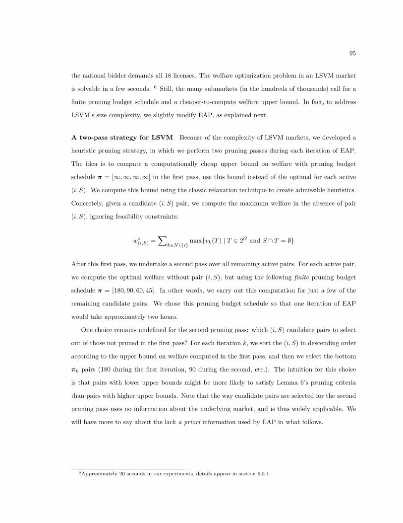
95

the national bidder demands all 18 licenses. The welfare optimization problem in an LSVM market

is solvable in a few seconds. 6 Still, the many submarkets (in the hundreds of thousands) call for a

finite pruning budget schedule and a cheaper-to-compute welfare upper bound. In fact, to address

LSVM’s size complexity, we slightly modify EAP, as explained next.

A two-pass strategy for LSVM Because of the complexity of LSVM markets, we developed a

heuristic pruning strategy, in which we perform two pruning passes during each iteration of EAP.

The idea is to compute a computationally cheap upper bound on welfare with pruning budget

schedule fi = [Œ, Œ, Œ, Œ] in the first pass, use this bound instead of the optimal for each active

(i, S). We compute this bound using the classic relaxation technique to create admissible heuristics.

Concretely, given a candidate (i, S) pair, we compute the maximum welfare in the absence of pair

(i, S), ignoring feasibility constraints:

wù(i,S) =

ÿkœN\{i}

max{vk(T ) | T œ 2G and S fl T = ÿ}

After this first pass, we undertake a second pass over all remaining active pairs. For each active pair,

we compute the optimal welfare without pair (i, S), but using the following finite pruning budget

schedule fi = [180, 90, 60, 45]. In other words, we carry out this computation for just a few of the

remaining candidate pairs. We chose this pruning budget schedule so that one iteration of EAP

would take approximately two hours.

One choice remains undefined for the second pruning pass: which (i, S) candidate pairs to select

out of those not pruned in the first pass? For each iteration k, we sort the (i, S) in descending order

according to the upper bound on welfare computed in the first pass, and then we select the bottom

fik pairs (180 during the first iteration, 90 during the second, etc.). The intuition for this choice

is that pairs with lower upper bounds might be more likely to satisfy Lemma 6’s pruning criteria

than pairs with higher upper bounds. Note that the way candidate pairs are selected for the second

pruning pass uses no information about the underlying market, and is thus widely applicable. We

will have more to say about the lack a priori information used by EAP in what follows.

6Approximately 20 seconds in our experiments, details appear in section 6.5.1.

96

GSV

MLS

VM

ÁEA

EAP

ÁE

AP

UM

Loss

EAEA

PÁ

EA

PU

MLo

ss

1.25

2,64

272

0±

100.

73±

0.01

0.00

22±

0.00

0233

0,49

7±

386

270,

754

±14

,15

40.

89±

0.00

0.00

11±

0.00

03

2.50

660

226

±10

1.57

±0.

020.

0041

±0.

0005

82,62

4±

9673

,73

3±

3,62

91.

78±

0.00

0.00

18±

0.00

03

5.00

165

117

±11

3.41

±0.

030.

0063

±0.

0008

20,65

6±

2422

,05

4±

933

3.59

±0.

010.

0037

±0.

0005

10.0

4169

±4

7.36

±0.

040.

0107

±0.

0010

5,16

4±

67,

580

±21

17.

27±

0.01

0.00

72±

0.00

11

Tabl

e6.

2:G

SVM

(left

grou

p)an

dLS

VM

(rig

htgr

oup)

resu

lts.

Each

grou

pre

port

ssa

mpl

ee�

cien

cyan

dU

Mlo

ss.

Each

row

ofth

eta

ble

repo

rts

resu

ltsfo

ra

fixed

valu

eof

Á.

Res

ults

are

95%

confi

denc

ein

terv

als

over

40G

SVM

mar

ket

draw

san

d50

LSV

Mm

arke

tdr

aws,

exce

ptfo

rEA

’snu

mbe

rof

sam

ples

inth

eca

seof

GSV

Mw

hich

isa

dete

rmin

istic

quan

tity

(aG

SVM

mar

ket

isof

size

4,48

0).

The

valu

esin

bold

indi

cate

the

mor

esa

mpl

ee�

cien

tal

gorit

hm.

Num

bers

ofsa

mpl

esar

ere

port

edin

mill

ions

.

97

Results. Table 6.2 summarizes the results of our experiments with GSVM and LSVM markets.

The table shows 95% confidence intervals around the mean number of samples needed by EA and

EAP to achieve the indicated accuracy (Á) guarantee for each row of the table. The table also shows

confidence intervals around the mean Á guarantees achieved by EAP, denoted ÁEAP, and confidence

intervals over the UM loss metric. Several observations follow.

Although ultimately a heuristic method, on average EAP uses far fewer samples than EA and

produces significantly better Á guarantees. We emphasize that EAP is capable of producing these

results without any a priori knowledge about the underlying market. Instead, EAP autonomously

samples those quantities that can provably be part of an optimal solution. The EAP guarantees

are slightly worse in the LSVM market than for GSVM, where we prune all eligible (i, S) pairs.

In general, there is a tradeo� between computational and sample e�ciency: at the cost of more

computation, to find more pairs to prune up front, one can save on future samples. Still, even

with a rather restricted pruning budget fi = [180, 90, 60, 45] (compared to hundreds of thousands

potentially active (i, S) pairs), EAP achieves substantial savings compared to EA in the LSVM

market.

Finally, the UM loss metric follows a trend similar to those observed for unit-demand markets,

i.e., the error guarantees are consistently met and degrade as expected (worst guarantees for higher

values of Á). Note that in our experiments, all 40 GSVM market instances have equilibria with linear

and anonymous prices. In contrast, only 18 out of 32 LSVM market do, so the table reports UM

loss over this set. For the remaining 32 markets, we report here a UM loss of approximately 12 ± 4

regardless of the value of Á. This high UM loss is due to the lack of CE in linear pricings which

dominates any UM loss attributable to the estimation of values.

98

6.5 Chapter Summary

In this chapter, we propose a simple extension of the standard model of combinatorial markets that

allows buyers’ values to be drawn from (possibly unknown) probability distributions. Even though

valuations are not known with complete certainty, we assume that noisy samples can be obtained,

for example, by using approximate methods, heuristics, or truncating the run-time of a complete

algorithm. For this model, we tackle the problem of learning CE. We first show tight lower- and

upper-bounds on the buyers’ utility loss, and hence the set of CE, given a uniform approximation

of one market by another. We then develop learning algorithms that, with high probability, learn

said uniform approximations using only finitely many samples.

Leveraging the first welfare theorem of economics, we define a pruning criterion under which

an algorithm can provably stop learning about buyers’ valuations for bundles, without a�ecting

the quality of the set of learned CE. We embed these conditions in an algorithm that we show

experimentally is capable of learning CE with far fewer samples than a baseline. Crucially, the

algorithm need not know anything about this structure a priori; our algorithm is general enough

to work in any combinatorial market. Moreover, we expect substantial improvement with sharper

sample complexity bounds; in particular, variance-sensitive bounds can be vastly more e�cient when

the variance is small, whereas Hoe�ding’s inequality essentially assumes the worst-case variance.

99

6.5.1 Experimental Technical Details

For our experiments, we solve for CE in linear prices. To compute CE in linear prices, we first

solve for a welfare-maximizing allocation yú and then, fixing y

ú, we solve for CE linear prices. Note

that, if a CE in linear prices exists, then it is supported by any welfare-maximizing allocation [110].

Moreover, since valuations in our experiments are drawn from continuous distributions, we assume

that the set of welfare-maximizing allocations for a given market is of negligible size.

Mathematical Programs Next, we present the mathematical programs we used to compute

welfare-maximizing allocations and find linear prices. Given a combinatorial market M, integer

linear program (6.14) [92] computes a welfare-maximizing allocation yú.

maximizeÿ

iœN,S™G

vi(S)xiS

subject toÿ

iœN,S|jœS

xiS Æ 1, j = 1, . . . , N

ÿ

S™G

xiS Æ 1, i = 1, . . . , n

xiS œ {0, 1}, i œ N, S ™ G

(6.14)

Given a market M and a solution yú to (6.14), the following set of linear inequalities, (6.15), define

all linear prices that couple with allocation yú to form a CE in M. The inequalities are defined over

variables P1, . . . , PN where Pj is good j’s price. The price of bundle S is thenq

jœS Pj .

vi(S) ≠q

jœS Pj Æ vi(Súi ) ≠

qjœSú

iPj , i œ N, S ™ G

If j /œ fiiœN Súi , then Pj = 0, j = 1, . . . , N

Pj Ø 0, j œ G

(6.15)

The first set of inequalities of (6.15) enforce the UM conditions. The second set of inequalities states

that the price of goods not allocated to any buyer in yú must be zero. In the case of linear pricing,

this condition is equivalent to the RM condition. In practice, a market might not have CE in linear

pricings, i.e., the set of feasible solutions of (6.15) might be empty. In our experiments, we solve

linear program (6.16), a relaxation of (6.15) where we introduce slack variables –iS to relax the UM

constraints. We define as objective function the sum of all slack variables,q

iœN,S™G –iS , which we

wish to minimize.

100

minimizeÿ

iœN,S™G

–iS

subject tovi(S) ≠

qjœS Pj ≠ –iS Æ vi(Sú

i ) ≠q

jœSúi

Pj , i œ N, S ™ G

If j /œ fiiœN Súi , then Pj = 0, j = 1, . . . , N

Pj Ø 0, j œ G

–iS Ø 0, i œ N, S ™ G

(6.16)

As reported in section 6.4.3, for each GSVM market we found that the optimal solution of (6.16) was

such thatq

iœN,S™G –iS = 0, which means that an exact CE in linear prices was found. In contrast,

for LSVM markets only 18 out of 50 markets had linear prices (q

iœN,S™G –iS = 0) whereas 32 did

not (q

iœN,S™G –iS > 0).

Further technical details We used the COIN-OR [114] library, through Python’s PuLP 7 inter-

face, to solve all mathematical programs. We wrote all our experiments in Python, and all code is

available at https://github.com/eareyan/noisyce. We ran our experiments in a cluster of two

Google’s GCloud c2-standard-4 machines. Unit-demand experiments took approximately two days

to complete, GSVM experiments approximately four days, and LSVM experiments approximately

eight days.

7https://pypi.org/project/PuLP/

https://github.com/eareyan/noisyce

https://pypi.org/project/PuLP/

Chapter 7

Conclusions and Future Directions

Our work contributed computational and statistical learning tools for analyzing and designing sys-

tems inhabited by multiple strategic agents. We first focused on developing and thoroughly evaluat-

ing methods that permit game-theoretic analysis of multi-agent systems whose complete description

is prohibitively expensive. Game-theoretic models of such systems are known as simulation-based

games because we only get to observe samples of utility functions by running the game’s simulator

but never a complete analytical description of them. We first proved tight bounds on the equilibria

error of a game’s uniform approximation and proposed algorithms that in practice e�ciently learn

said uniform approximations for simulation-based games. In extensive experimentation, we showed

that our algorithms produce high-quality uniform approximations that preserve the game’s equilibria

making frugal use of data or calls of the game’s simulator – a major computational bottleneck when

analyzing simulation-based games in practice.

Equipped with algorithms capable of learning the equilibria of simulation-based games, we intro-

duced a methodology to optimize the performance of multi-agent systems given a designer’s objective

function – a well-defined success metric mapping a state of the system to a number. Our methods

formalize the design of mechanisms as a search problem within the parameter space of an overall

parameterized mechanism. For example, when auctioning online advertisements, an advertisement

exchange’s goal is to maximize its revenue by setting reserve prices, i.e., prices below which it will

not allocate ads. The challenge then is to find a set of reserve prices such that, at equilibrium,

the ad exchange maximizes its revenue. In addition to facing a massive search space, this task is

challenging because the ad exchange does not have access to agents’ strategies but only to samples of

101

102

their behavior. Having access only to samples of agent’s behavior is a feature of modern multi-agent

systems, and we believe our methodological contributions are a step towards their e�cient analysis.

To evaluate our empirical mechanism design methodology, we developed a stylized-but-rich model

of an electronic advertisement exchange’s dynamics, paying particular attention to the exchange’s

ability to set di�erent reserve prices based on user demographic data. Since the quality of the reserve

prices found via our empirical mechanism design methods depends on the quality of the heuristic

strategies used to find them in the first place, we further contributed two heuristic bidding strategies

for our ad exchange model. Crucially, these heuristics are responsive to di�erent reserve price choices

by the ad exchange, allowing us to simulate sophisticated bidders’ behavior. We showed that our

empirical mechanism design methodology recovers optimal mechanisms when they are known more

e�ciently than existing baselines. For our ad exchange model, we experimentally demonstrated that

our methods produce reserve prices that, at equilibrium, yield higher revenue more e�ciently (with

fewer samples) than standard baselines.

Ad exchanges are one example of a broader class of markets known as combinatorial markets. In

a combinatorial market, goods are indivisible, meaning that a seller must allocate each good entirely

to a single buyer. These markets are pervasive and fundamental to modern economies; examples

include the allocation of online advertisement, the allocation of rights to use radio spectrum, etc.

The combinatorial nature of buyers’ preferences complicates their analysis, particularly buyers’ abil-

ity to completely characterize their preferences in the presence of exponentially many bundles of

goods. Our final contribution is a simple but powerful model that allows buyers to express their

uncertainty over bundles of goods and learning algorithms that, with high probability, preserve the

market’s approximate competitive equilibria where the approximation error is a function of buyer’s

uncertainty over bundles of goods. Extensive experimentation on spectrum auction value models

shows the e�cacy of our learning algorithms. Moreover, our experiments illustrate the various trade-

o�s a market maker faces between an outcome’s quality and the required amount of computational

resources when implementing a market for which bidders have uncertain values.

Much work remains to make the methods developed in this thesis fully usable in practice. We

hope that this thesis e�ectively introduced key theoretical and experimental insights that researchers

can build upon to make further contributions of their own and eventually products and services that

improve quality of life everywhere.

We conclude by pointing out future research directions we believe will lead to fruitful results.

103

Future WorkOur work opens new and exciting future research directions. We mention some of them next.

Equilibria Subset. In our work, we paid particular attention to algorithms that rigorously learn,

up to some user-desired approximation error, a simulation-based game’s equilibria set, or a noisy

combinatorial market’s competitive equilibria set. A consequence of this choice is that, in practice,

our methods sometimes require a prohibitively large number of samples. One possibility to lessen this

high-sampling requirement would be to adapt our methods to learn only some equilibria subset. The

challenge would be to identify relevant parts of the equilibria space and discard the rest. Another

possibility would be to relax the method’s rigorousness and instead settle for weaker guarantees

achievable with fewer samples and computational resources.

Heuristic concentration inequalities. Empirically, we found that concentration inequalities such

as Hoe�ding’s or Bennett’s are often too pessimistic in the number of samples they require. In

practice, over the set of games we tested, the number of samples needed for these inequalities to

retain strict guarantees on learned games or mechanisms’ quality is far superior to the actual number

of samples necessary. While this phenomenon might be due to our sometimes admittedly simple noise

models, an interesting future direction would be to investigate heuristic relaxations of these worst-

case inequalities and evaluate them in practice. Said practical evaluation would require designing

more sophisticated noise models or collecting samples directly from real-world applications, both of

which we believe are fruitful research directions.

Simulation-based game-theoretic solution concepts. Our current empirical mechanism design uses

a parameterized simulation-based game’s strongly connected components to predict agents’ behav-

ior. While the strongly connected components are statistically and computationally tractable, work

remains to evaluate their predictive power in simulation-based games. Furthermore, the strongly

connected components are a relaxation of sink equilibria itself statistically intractable but computa-

tionally tractable. The question remains whether we can find other solution concepts “in-between”

the strongly connected components and sink equilibria that are both computationally and statisti-

cally tractable. It would also be worthwhile to investigate di�erent solution concepts, e.g., correlated

equilibria, and their applicability in our empirical mechanism design methodology.

Empirical mechanism design by competitive equilibria. Finally, when designing combinatorial

markets, an alternative to learning game-theoretic solution concepts for agent’s predictive behavior

would be to learn competitive equilibria as demonstrated in chapter 6.

Bibliography

[1] amazon.com. Amazon display ads. https://advertising.amazon.com/products/

display-ads, 2020. Accessed: 2020-04-05.

[2] amazon.com. Amazon sponsored products. https://advertising.amazon.com/products/

sponsored-products, 2020. Accessed: 2020-04-05.

[3] E. Areyan Viqueira. Principled autonomous decision making for markets. In Proceedings of

the 16th Conference on Autonomous Agents and MultiAgent Systems, pages 1869–1870, 2017.

[4] E. Areyan Viqueira, A. Greenwald, and V. Naroditskiy. On approximate welfare-and revenue-

maximizing equilibria for size-interchangeable bidders. In Proceedings of the 16th Conference

on Autonomous Agents and MultiAgent Systems, pages 1466–1468. International Foundation

for Autonomous Agents and Multiagent Systems, 2017.

[5] E. Areyan Viqueira, A. Greenwald, and V. Naroditskiy. On approximate welfare-and revenue-

maximizing equilibria for size-interchangeable bidders. arXiv preprint arXiv:1708.03097, 2017.

[6] E. Areyan Viqueira, C. Cousins, E. Upfal, and A. Greenwald. Learning equilibria of simulation-

based games. arXiv preprint arXiv:1905.13379, 2019.

[7] E. Areyan Viqueira, A. Greenwald, C. Cousins, and E. Upfal. Learning simulation-based games

from data. In Proceedings of the 18th International Conference on Autonomous Agents and

MultiAgent Systems, pages 1778–1780. International Foundation for Autonomous Agents and

Multiagent Systems, 2019.

[8] E. Areyan Viqueira, C. Cousins, and A. Greenwald. Improved algorithms for learning equilibria

in simulation-based games. In Proceedings of the 19th International Conference on Autonomous

Agents and MultiAgent Systems, pages 79–87, 2020.

104

https://advertising.amazon.com/products/display-ads

https://advertising.amazon.com/products/display-ads

https://advertising.amazon.com/products/sponsored-products

https://advertising.amazon.com/products/sponsored-products

105

[9] E. Areyan Viqueira, C. Cousins, and A. Greenwald. Learning competitive equilibria in noisy

combinatorial markets. In Proceedings of the 20th International Conference on Autonomous

Agents and MultiAgent Systems, 2021.

[10] J.-Y. Audibert, R. Munos, and C. Szepesvári. Tuning bandit algorithms in stochastic environ-

ments. In International conference on algorithmic learning theory, pages 150–165. Springer,

2007.

[11] J.-Y. Audibert, R. Munos, and C. Szepesvári. Variance estimates and exploration function in

multi-armed bandit. In CERTIS Research Report 07–31. Citeseer, 2007.

[12] M. Babaio�, N. Nisan, and R. Paes Leme. Price competition in online combinatorial markets.

In Proceedings of the 23rd international conference on World wide web, pages 711–722, 2014.

[13] M. Balcan and N. J. A. Harvey. Learning submodular functions. In L. Fortnow and S. P.

Vadhan, editors, Proceedings of the 43rd ACM Symposium on Theory of Computing, STOC

2011, San Jose, CA, USA, 6-8 June 2011, pages 793–802. ACM, 2011. doi: 10.1145/1993636.

1993741. URL https://doi.org/10.1145/1993636.1993741.

[14] M. Balcan, F. Constantin, S. Iwata, and L. Wang. Learning valuation functions. In S. Mannor,

N. Srebro, and R. C. Williamson, editors, COLT 2012 - The 25th Annual Conference on

Learning Theory, June 25-27, 2012, Edinburgh, Scotland, volume 23 of JMLR Proceedings,

pages 4.1–4.24. JMLR.org, 2012. URL http://proceedings.mlr.press/v23/balcan12b/

balcan12b.pdf.

[15] M. Ball, G. Donohue, and K. Ho�man. Auctions for the safe, e�cient, and equitable allocation

of airspace system resources. Combinatorial auctions, 1, 2006.

[16] Y. Bartal, R. Gonen, and N. Nisan. Incentive compatible multi unit combinatorial auctions.

In Proceedings of the 9th conference on Theoretical aspects of rationality and knowledge, pages

72–87, 2003.

[17] P. L. Bartlett and S. Mendelson. Rademacher and gaussian complexities: Risk bounds and

structural results. Journal of Machine Learning Research, 3(Nov):463–482, 2002.

[18] D. R. Bellhouse, N. Fillion, et al. Le her and other problems in probability discussed by

bernoulli, montmort and waldegrave. Statistical Science, 30(1):26–39, 2015.

https://doi.org/10.1145/1993636.1993741

http://proceedings.mlr.press/v23/balcan12b/balcan12b.pdf

http://proceedings.mlr.press/v23/balcan12b/balcan12b.pdf

106

[19] G. Bennett. Probability inequalities for the sum of independent random variables. Journal of

the American Statistical Association, 57(297):33–45, 1962.

[20] J. Bergstra and Y. Bengio. Random search for hyper-parameter optimization. Journal of

Machine Learning Research, 13(Feb):281–305, 2012.

[21] S. Bikhchandani and J. W. Mamer. Competitive equilibrium in an exchange economy with

indivisibilities. Journal of economic theory, 74(2):385–413, 1997.

[22] S. Bikhchandani, J. M. Ostroy, et al. The package assignment model. Journal of Economic

theory, 107(2):377–406, 2002.

[23] V. Bilò, M. Flammini, G. Monaco, and L. Moscardelli. On the impact of buyers preselection in

pricing problems. In Proceedings of the 17th International Conference on Autonomous Agents

and MultiAgent Systems, pages 1871–1873. International Foundation for Autonomous Agents

and Multiagent Systems, 2018.

[24] V. Bilò, M. Flammini, G. Monaco, and L. Moscardelli. Pricing problems with buyer prese-

lection. In 43rd International Symposium on Mathematical Foundations of Computer Science

(MFCS 2018). Schloss Dagstuhl-Leibniz-Zentrum fuer Informatik, 2018.

[25] L. Blumrosen and N. Nisan. Combinatorial auctions. Algorithmic game theory, 267:300, 2007.

[26] T. Börgers. An introduction to the theory of mechanism design. Oxford University Press, USA,

2015.

[27] S. Boucheron, G. Lugosi, and P. Massart. Concentration inequalities: A nonasymptotic theory

of independence. Oxford university press, 2013.

[28] E. Budish. The combinatorial assignment problem: Approximate competitive equilibrium from

equal incomes. Journal of Political Economy, 119(6):1061–1103, 2011.

[29] E. Cantillon and M. Pesendorfer. Auctioning bus routes: The london experience. ., 2006.

[30] M. Cary, A. Das, B. Edelman, I. Giotis, K. Heimerl, A. R. Karlin, C. Mathieu, and M. Schwarz.

Greedy bidding strategies for keyword auctions. In Proceedings of the 8th ACM conference on

Electronic commerce, pages 262–271. ACM, 2007.

107

[31] Y. Chen, S. Goel, and D. M. Pennock. Pricing combinatorial markets for tournaments. In

Proceedings of the fortieth annual ACM symposium on Theory of computing, pages 305–314,

2008.

[32] Y. K. Cheung, R. Cole, and N. R. Devanur. Tatonnement beyond gross substitutes? gradient

descent to the rescue. Games and Economic Behavior, 123:295–326, 2020.

[33] E. H. Clarke. Multipart pricing of public goods. Public choice, pages 17–33, 1971.

[34] W. Conen and T. Sandholm. Preference elicitation in combinatorial auctions. In M. P. Wellman

and Y. Shoham, editors, Proceedings 3rd ACM Conference on Electronic Commerce (EC-2001),

Tampa, Florida, USA, October 14-17, 2001, pages 256–259. ACM, 2001. doi: 10.1145/501158.

501191. URL https://doi.org/10.1145/501158.501191.

[35] V. Conitzer and T. Sandholm. An algorithm for automatically designing deterministic mech-

anisms without payments. In Proceedings of the Third International Joint Conference on

Autonomous Agents and Multiagent Systems, 2004. AAMAS 2004., pages 128–135. IEEE,

2004.

[36] P. Cramton et al. Spectrum auctions. Handbook of telecommunications economics, 1:605–639,

2002.

[37] R. W. Crandall. New zealand spectrum policy: A model for the united states? The Journal

of Law and Economics, 41(S2):821–840, 1998.

[38] R. K. Dash, N. R. Jennings, and D. C. Parkes. Computational-mechanism design: A call to

arms. IEEE intelligent systems, 18(6):40–47, 2003.

[39] C. Daskalakis, P. W. Goldberg, and C. H. Papadimitriou. The complexity of computing a

nash equilibrium. SIAM Journal on Computing, 39(1):195–259, 2009.

[40] S. De Vries and R. V. Vohra. Combinatorial auctions: A survey. INFORMS Journal on

computing, 15(3):284–309, 2003.

[41] B. Edelman, M. Ostrovsky, and M. Schwarz. Internet advertising and the generalized second-

price auction: Selling billions of dollars worth of keywords. American economic review, 97(1):

242–259, 2007.

https://doi.org/10.1145/501158.501191

108

[42] T. Elomaa and M. Kääriäinen. Progressive Rademacher sampling. In AAAI/IAAI, pages

140–145, 2002.

[43] E. Even Dar, V. S. Mirrokni, S. Muthukrishnan, Y. Mansour, and U. Nadav. Bid optimization

for broad match ad auctions. In Proceedings of the 18th international conference on World

wide web, pages 231–240. ACM, 2009.

[44] M. Feldman, N. Gravin, and B. Lucier. Combinatorial walrasian equilibrium. SIAM Journal

on Computing, 45(1):29–48, 2016.

[45] Y. Fujishima, K. Leyton-Brown, and Y. Shoham. Taming the computational complexity of

combinatorial auctions: Optimal and approximate approaches. In T. Dean, editor, Proceedings

of the Sixteenth International Joint Conference on Artificial Intelligence, IJCAI 99, Stockholm,

Sweden, July 31 - August 6, 1999. 2 Volumes, 1450 pages, pages 548–553. Morgan Kaufmann,

1999. URL http://ijcai.org/Proceedings/99-1/Papers/079.pdf.

[46] D. Gale. Equilibrium in a discrete exchange economy with money. International Journal of

Game Theory, 13(1):61–64, 1984.

[47] D. Gale and L. S. Shapley. College admissions and the stability of marriage. The American

Mathematical Monthly, 69(1):9–15, 1962.

[48] R. Garg, S. Kapoor, and V. Vazirani. An auction-based market equilibrium algorithm for the

separable gross substitutability case. In Approximation, Randomization, and Combinatorial

Optimization. Algorithms and Techniques, pages 128–138. Springer, 2004.

[49] N. Gatti and M. Restelli. Equilibrium approximation in simulation-based extensive-form

games. In The 10th International Conference on Autonomous Agents and Multiagent Sys-

tems - Volume 1, AAMAS ’11, page 199–206, Richland, SC, 2011. International Foundation

for Autonomous Agents and Multiagent Systems. ISBN 0982657153.

[50] S. Gerakaris and S. Ramamoorthy. Learning best response strategies for agents in ad ex-

changes. In European Conference on Multi-Agent Systems, pages 77–93. Springer, 2018.

[51] R. Gibbons. Game theory for applied economists. Princeton University Press, 1992.

http://ijcai.org/Proceedings/99-1/Papers/079.pdf

109

[52] M. Goemans, V. Mirrokni, and A. Vetta. Sink equilibria and convergence. In Foundations

of Computer Science, 2005. FOCS 2005. 46th Annual IEEE Symposium on, pages 142–151.

IEEE, 2005.

[53] J. K. Goeree and C. A. Holt. Hierarchical package bidding: A paper & pencil combinatorial

auction. Games and Economic Behavior, 70(1):146–169, 2010.

[54] S. Govindan and R. Wilson. A global newton method to compute nash equilibria. Journal of

Economic Theory, 110(1):65–86, 2003.

[55] S. Govindan and R. Wilson. Computing nash equilibria by iterated polymatrix approximation.

Journal of Economic Dynamics and Control, 28(7):1229–1241, 2004.

[56] A. Greenwald, V. Naroditskiy, and S. J. Lee. Bidding heuristics for simultaneous auctions:

Lessons from tac travel. In Agent-Mediated Electronic Commerce and Trading Agent Design

and Analysis, pages 131–146. Springer, 2010.

[57] T. Groves. Incentives in teams. Econometrica: Journal of the Econometric Society, pages

617–631, 1973.

[58] F. Gul and E. Stacchetti. Walrasian equilibrium with gross substitutes. Journal of Economic

theory, 87(1):95–124, 1999.

[59] M. Guo and V. Conitzer. Computationally feasible automated mechanism design: General

approach and case studies. In Twenty-Fourth AAAI Conference on Artificial Intelligence,

2010.

[60] V. Guruswami, J. D. Hartline, A. R. Karlin, D. Kempe, C. Kenyon, and F. McSherry. On profit-

maximizing envy-free pricing. In Proceedings of the sixteenth annual ACM-SIAM symposium

on Discrete algorithms, pages 1164–1173. Society for Industrial and Applied Mathematics,

2005.

[61] O. Hinz, I.-H. Hann, and M. Spann. Price discrimination in e-commerce? an examination of

dynamic pricing in name-your-own price markets. Mis quarterly, pages 81–98, 2011.

[62] W. Hoe�ding. Probability inequalities for sums of bounded random variables. Journal of the

American statistical association, 58(301):13–30, 1963.

110

[63] iab.com. U.s. digital ad revenue climbs to $57.9 billion in first half 2019, up 17%

yoy, according to iab internet advertising revenue report. https://www.iab.com/news/

u-s-digital-ad-revenue-climbs-to-57-9-billion-in-first-half-2019/, 2020. Ac-

cessed: 2020-05-09.

[64] T. Jha and Y. Zick. A learning framework for distribution-based game-theoretic solution

concepts. In Proceedings of the 21st ACM Conference on Economics and Computation, pages

355–377, 2020.

[65] P. R. Jordan and M. P. Wellman. Designing an ad auctions game for the trading agent compe-

tition. In Agent-Mediated Electronic Commerce. Designing Trading Strategies and Mechanisms

for Electronic Markets. Springer, 2010.

[66] P. R. Jordan, C. Kiekintveld, and M. P. Wellman. Empirical game-theoretic analysis of the tac

supply chain game. In Proceedings of the 6th international joint conference on Autonomous

agents and multiagent systems, page 193. ACM, 2007.

[67] P. R. Jordan, Y. Vorobeychik, and M. P. Wellman. Searching for approximate equilibria in

empirical games. In Proceedings of the 7th international joint conference on Autonomous agents

and multiagent systems-Volume 2, pages 1063–1070. International Foundation for Autonomous

Agents and Multiagent Systems, 2008.

[68] M. Kaneko and Y. Yamamoto. The existence and computation of competitive equilibria in

markets with an indivisible commodity. Journal of Economic Theory, 38(1):118–136, 1986.

[69] A. S. Kelso Jr and V. P. Crawford. Job matching, coalition formation, and gross substitutes.

Econometrica: Journal of the Econometric Society, pages 1483–1504, 1982.

[70] W. Ketter, M. Peters, and J. Collins. Autonomous agents in future energy markets: The 2012

power trading agent competition. In AAAI, 2013.

[71] D. Koller, N. Megiddo, and B. Von Stengel. E�cient computation of equilibria for extensive

two-person games. Games and economic behavior, 14(2):247–259, 1996.

[72] V. Koltchinskii. Rademacher penalties and structural risk minimization. IEEE Transactions

on Information Theory, 47(5):1902–1914, 2001.

https://www.iab.com/news/u-s-digital-ad-revenue-climbs-to-57-9-billion-in-first-half-2019/

https://www.iab.com/news/u-s-digital-ad-revenue-climbs-to-57-9-billion-in-first-half-2019/

111

[73] V. Krishna. Auction theory. Academic press, 2009.

[74] C. Kroer, A. Peysakhovich, E. Sodomka, and N. E. S. Moses. Computing large market

equilibria using abstractions. In A. Karlin, N. Immorlica, and R. Johari, editors, Proceed-

ings of the 2019 ACM Conference on Economics and Computation, EC 2019, Phoenix, AZ,

USA, June 24-28, 2019, pages 745–746. ACM, 2019. doi: 10.1145/3328526.3329553. URL

https://doi.org/10.1145/3328526.3329553.

[75] H. W. Kuhn. The hungarian method for the assignment problem. Naval research logistics

quarterly, 2(1-2):83–97, 1955.

[76] A. M. Kwasnica, J. O. Ledyard, D. Porter, and C. DeMartini. A new and improved design for

multiobject iterative auctions. Management science, 51(3):419–434, 2005.

[77] S. Lahaie and B. Lubin. Adaptive-price combinatorial auctions. In A. Karlin, N. Immorlica, and

R. Johari, editors, Proceedings of the 2019 ACM Conference on Economics and Computation,

EC 2019, Phoenix, AZ, USA, June 24-28, 2019, pages 749–750. ACM, 2019. doi: 10.1145/

3328526.3329615. URL https://doi.org/10.1145/3328526.3329615.

[78] S. Lahaie and D. C. Parkes. Applying learning algorithms to preference elicitation. In J. S.

Breese, J. Feigenbaum, and M. I. Seltzer, editors, Proceedings 5th ACM Conference on Elec-

tronic Commerce (EC-2004), New York, NY, USA, May 17-20, 2004, pages 180–188. ACM,

2004. doi: 10.1145/988772.988800. URL https://doi.org/10.1145/988772.988800.

[79] B. Lehmann, D. Lehmann, and N. Nisan. Combinatorial auctions with decreasing marginal

utilities. Games and Economic Behavior, 55(2):270–296, 2006.

[80] K. Leyton-Brown, E. Nudelman, and Y. Shoham. Learning the empirical hardness of optimiza-

tion problems: The case of combinatorial auctions. In International Conference on Principles

and Practice of Constraint Programming, pages 556–572. Springer, 2002.

[81] B. Lubin and D. C. Parkes. Combinatorial markets in theory and practice: Mitigating incen-

tives and facilitating elicitation. Citeseer, 2010.

[82] J. K. MacKie-Mason, A. Osepayshvili, D. M. Reeves, and M. P. Wellman. Price prediction

strategies for market-based scheduling. AAAI, 2004.

https://doi.org/10.1145/3328526.3329553

https://doi.org/10.1145/3328526.3329615

https://doi.org/10.1145/988772.988800

112

[83] magnaglobal.com. Global advertising forecast. https://www.magnaglobal.com/wp-content/

uploads/2016/12/MAGNA-December-Global-Forecast-Update-Press-Release.pdf, 2017.

Accessed: 2017-11-15.

[84] A. Marchesi, F. Trovò, and N. Gatti. Learning Probably Approximately Correct Maximin

Strategies in Simulation-Based Games with Infinite Strategy Spaces, page 834–842. Interna-

tional Foundation for Autonomous Agents and Multiagent Systems, Richland, SC, 2020. ISBN

9781450375184.

[85] A. Maurer and M. Pontil. Empirical bernstein bounds and sample variance penalization. arXiv

preprint arXiv:0907.3740, 2009.

[86] R. McKelvey, A. McLennan, and T. Turocy. Gambit: Software tools for game theory, version

16.0.1., 2019. URL http://www.gambit-project.org.

[87] Y. Mohammad, E. A. Viqueira, N. A. Ayerza, A. Greenwald, S. Nakadai, and S. Morinaga.

Supply chain management world. In International Conference on Principles and Practice of

Multi-Agent Systems, pages 153–169. Springer, 2019.

[88] R. B. Myerson. Optimal auction design. Mathematics of operations research, 6(1):58–73, 1981.

[89] R. B. Myerson. Game theory. Harvard university press, 2013.

[90] J. F. Nash. Equilibrium points in n-person games. Proceedings of the national academy of

sciences, 1950.

[91] N. Nisan and A. Ronen. Algorithmic mechanism design. Games and Economic behavior, 35

(1-2):166–196, 2001.

[92] N. Nisan, T. Roughgarden, E. Tardos, and V. V. Vazirani. Algorithmic game theory, 2007.

Google Scholar Google Scholar Digital Library Digital Library, 2007.

[93] E. Nudelman, J. Wortman, Y. Shoham, and K. Leyton-Brown. Run the gamut: A compre-

hensive approach to evaluating game-theoretic algorithms. In Proceedings of the Third Inter-

national Joint Conference on Autonomous Agents and Multiagent Systems-Volume 2, pages

880–887. IEEE Computer Society, 2004.

https://www.magnaglobal.com/wp-content/uploads/2016/12/MAGNA-December-Global-Forecast-Update-Press-Release.pdf

https://www.magnaglobal.com/wp-content/uploads/2016/12/MAGNA-December-Global-Forecast-Update-Press-Release.pdf

http://www.gambit-project.org.

113

[94] J. O’Donovan, R. Jones, L. R. Marusich, Y. Teng, C. Gonzalez, and T. Höllerer. A model-

based evaluation of trust and situation awareness in the diner’s dilemma game. In Proceedings

of the 22th Behavior Representation in Modeling & Simulation (BRIMS) Conference, pages

11–14, 2013.

[95] D. C. Parkes. Iterative combinatorial auctions. MIT press, 2006.

[96] D. C. Parkes. Computational mechanism design. In Lecture Notes of Tutorials Presented at the

10th Conference on Theoretical Aspects of Rationality and Knowledge (TARK-05). Institute

of Mathematical Sciences, University of Singapore, 2008.

[97] D. C. Parkes. When analysis fails: Heuristic mechanism design via self-correcting procedures.

In International Conference on Current Trends in Theory and Practice of Computer Science,

pages 62–66. Springer, 2009.

[98] S. Phelps, S. Parsons, P. McBurney, and E. Sklar. Co-evolution of auction mechanisms and

trading strategies: Towards a novel approach to microeconomic design. In In GECCO-02

Workshop on Evolutionary Computation in Multi-Agent Systems. Citeseer, 2002.

[99] S. Phelps, S. Parsons, E. Sklar, and P. McBurney. Using genetic programming to optimise

pricing rules for a double auction market. In Proceedings of the workshop on Agents for

Electronic Commerce, 2003.

[100] V. Picheny, M. Binois, and A. Habbal. A bayesian optimization approach to find nash equi-

libria. arXiv preprint arXiv:1611.02440, 2016.

[101] T. Popoviciu. Sur les équations algébriques ayant toutes leurs racines réelles. Mathematica, 9:

129–145, 1935.

[102] R. Porter, E. Nudelman, and Y. Shoham. Simple search methods for finding a nash equilibrium.

Games and Economic Behavior, 63(2):642–662, 2008.

[103] C. E. Rasmussen. Gaussian processes in machine learning. In Summer School on Machine

Learning, pages 63–71. Springer, 2003.

[104] M. Riondato and E. Upfal. Mining frequent itemsets through progressive sampling with

Rademacher averages. In Proceedings of the 21th ACM SIGKDD International Conference

on Knowledge Discovery and Data Mining, pages 1005–1014. ACM, 2015.

114

[105] M. Riondato and E. Upfal. Abra: Approximating betweenness centrality in static and dynamic

graphs with Rademacher averages. ACM Transactions on Knowledge Discovery from Data

(TKDD), 12(5):61, 2018.

[106] A. E. Roth. On the allocation of residents to rural hospitals: a general property of two-sided

matching markets. Econometrica: Journal of the Econometric Society, pages 425–427, 1986.

[107] A. E. Roth. Deferred acceptance algorithms: History, theory, practice, and open questions.

international Journal of game Theory, 36(3-4):537–569, 2008.

[108] A. E. Roth and M. Sotomayor. Two-sided matching. Handbook of game theory with economic

applications, 1:485–541, 1992.

[109] T. Roughgarden. Algorithmic game theory. Commun. ACM, 53(7):78–86, 2010. doi: 10.1145/

1785414.1785439. URL https://doi.org/10.1145/1785414.1785439.

[110] T. Roughgarden and I. Talgam-Cohen. Why prices need algorithms. In T. Roughgarden,

M. Feldman, and M. Schwarz, editors, Proceedings of the Sixteenth ACM Conference on Eco-

nomics and Computation, EC ’15, Portland, OR, USA, June 15-19, 2015, pages 19–36. ACM,

2015. doi: 10.1145/2764468.2764515. URL https://doi.org/10.1145/2764468.2764515.

[111] A. Rubinstein. Perfect equilibrium in a bargaining model. Econometrica: Journal of the

Econometric Society, pages 97–109, 1982.

[112] N. Sadeh, R. Arunachalam, J. Eriksson, N. Finne, and S. Janson. Tac-03–a supply-chain

trading competition. AI magazine, 24(1):92, 2003.

[113] F. Sailer, M. Buro, and M. Lanctot. Adversarial planning through strategy simulation. In

2007 IEEE symposium on computational intelligence and games, pages 80–87. IEEE, 2007.

[114] M. J. Saltzman. Coin-or: an open-source library for optimization. In Programming languages

and systems in computational economics and finance, pages 3–32. Springer, 2002.

[115] T. Sandholm. Automated mechanism design: A new application area for search algorithms. In

International Conference on Principles and Practice of Constraint Programming, pages 19–36.

Springer, 2003.

https://doi.org/10.1145/1785414.1785439

https://doi.org/10.1145/2764468.2764515

115

[116] M. Schain and Y. Mansour. Ad exchange–proposal for a new trading agent competition game.

In Agent-Mediated Electronic Commerce. Designing Trading Strategies and Mechanisms for

Electronic Markets, pages 133–145. Springer, 2013.

[117] T. Sche�el, G. Ziegler, and M. Bichler. On the impact of package selection in combinatorial

auctions: an experimental study in the context of spectrum auction design. Experimental

Economics, 15(4):667–692, 2012.

[118] J. Snoek, H. Larochelle, and R. P. Adams. Practical bayesian optimization of machine learning

algorithms. In Advances in neural information processing systems, pages 2951–2959, 2012.

[119] R. Tarjan. Depth-first search and linear graph algorithms. SIAM journal on computing, 1(2):

146–160, 1972.

[120] A. Tavares, H. Azpurua, A. Santos, and L. Chaimowicz. Rock, paper, starcraft: Strategy se-

lection in real-time strategy games. In The Twelfth AAAI Conference on Artificial Intelligence

and Interactive Digital Entertainment (AIIDE-16), 2016.

[121] K. Tuyls, J. Perolat, M. Lanctot, J. Z. Leibo, and T. Graepel. A generalised method for

empirical game theoretic analysis. arXiv preprint arXiv:1803.06376, 2018.

[122] K. Tuyls, J. Perolat, M. Lanctot, E. Hughes, R. Everett, J. Z. Leibo, C. Szepesvári, and

T. Graepel. Bounds and dynamics for empirical game theoretic analysis. Autonomous Agents

and Multi-Agent Systems, 34(1):7, 2020.

[123] L. G. Valiant. A theory of the learnable. Communications of the ACM, 27(11):1134–1142,

1984.

[124] W. Vickrey. Counterspeculation, auctions, and competitive sealed tenders. The Journal of

finance, 16(1):8–37, 1961.

[125] E. A. Viqueira, C. Cousins, Y. Mohammad, and A. Greenwald. Parametric mechanism design

under uncertainty. In To Appear on the Thirty-Fifth Conference on Uncertainty in Artificial

Intelligence, UAI 2019, Tel Aviv, Israel, July 22-25, 2019, 2019.

[126] E. A. Viqueira, C. Cousins, and A. Greenwald. Learning competitive equilibria in noisy

combinatorial markets. arXiv preprint arXiv:2101.09551, 2021.

116

[127] J. Von Neumann, O. Morgenstern, and H. W. Kuhn. Theory of games and economic behavior

(commemorative edition). Princeton university press, 2007.

[128] Y. Vorobeychik. Probabilistic analysis of simulation-based games. ACM Transactions on

Modeling and Computer Simulation (TOMACS), 20(3):16, 2010.

[129] Y. Vorobeychik and M. P. Wellman. Stochastic search methods for nash equilibrium approxi-

mation in simulation-based games. In Proceedings of the 7th international joint conference on

Autonomous agents and multiagent systems-Volume 2, pages 1055–1062. International Foun-

dation for Autonomous Agents and Multiagent Systems, 2008.

[130] Y. Vorobeychik, C. Kiekintveld, and M. P. Wellman. Empirical mechanism design: methods,

with application to a supply-chain scenario. In Proceedings of the 7th ACM conference on

Electronic commerce. ACM, 2006.

[131] Y. Vorobeychik, M. P. Wellman, and S. Singh. Learning payo� functions in infinite games.

Machine Learning, 67(1-2):145–168, 2007.

[132] L. Walras. Elements of Pure Economics: Or the Theory of Social Wealth. Elements of Pure

Economics, Or the Theory of Social Wealth. Routledge, 2003. ISBN 9780415313407. URL

https://books.google.com/books?id=hwjRD3z0Qy4C.

[133] M. Weiss, B. Lubin, and S. Seuken. Sats: A universal spectrum auction test suite. In Pro-

ceedings of the 16th Conference on Autonomous Agents and MultiAgent Systems, pages 51–59.

International Foundation for Autonomous Agents and Multiagent Systems, 2017.

[134] M. P. Wellman. Methods for empirical game-theoretic analysis. In AAAI, pages 1552–1556,

2006.

[135] M. P. Wellman. Trading agents. Synthesis Lectures on Artificial Intelligence and Machine

Learning, 5(3):1–107, 2011.

[136] M. P. Wellman, P. R. Jordan, C. Kiekintveld, J. Miller, and D. M. Reeves. Empirical game-

theoretic analysis of the tac market games. In AAMAS-06 Workshop on Game-Theoretic and

Decision-Theoretic Agents, volume 10, 2006.

[137] M. P. Wellman, A. Greenwald, and P. Stone. Autonomous bidding agents: Strategies and

lessons from the trading agent competition. Mit Press, 2007.

https://books.google.com/books?id=hwjRD3z0Qy4C

117

[138] M. P. Wellman, T. H. Kim, and Q. Duong. Analyzing incentives for protocol compliance in

complex domains: A case study of introduction-based routing. arXiv preprint arXiv:1306.0388,

2013.

[139] B. Wiedenbeck. Approximate game theoretic analysis for large simulation-based games.

In Proceedings of the 2014 International Conference on Autonomous Agents and Multi-

agent Systems, AAMAS ’14, pages 1745–1746, Richland, SC, 2014. International Foun-

dation for Autonomous Agents and Multiagent Systems. ISBN 978-1-4503-2738-1. URL

http://dl.acm.org/citation.cfm?id=2615731.2616156.

[140] B. Wiedenbeck, F. Yang, and M. P. Wellman. A regression approach for modeling games with

many symmetric players. In 32nd AAAI Conference on Artificial Intelligence, 2018.

[141] S. Zamir et al. Bayesian games: Games with incomplete information. Technical report, N/A,

2008.

[142] B. H. Zhang and T. Sandholm. Finding and certifying (near-) optimal strategies in black-box

extensive-form games. arXiv preprint arXiv:2009.07384, 2020.

http://dl.acm.org/citation.cfm?id=2615731.2616156

Documents

samples of utility functions but never a complete analytical