SAMPLING TECHNIQUES FORMEASURING AND FORECASTING

CROP YIELDS

rc ECONOMICS, STATISTICS, AND_ COOPERATIVES SERVICE

u.s. DEPARTMENTOF AGRICULTURE

ESCSNo. 09

SAMPLING TECHNIQUES FOR

MEASURING AND FORECASTING CROP YIELDS

By

Harold F. HuddlestonEconomics, Statistics, and Cooperatives Service

U.S. Departmentof Agriculture

August 1978

PREFACE

The purpose of this manual is to call attention to some of thesampling techniques for estimating crop yields. Many of the impor-tant changes that have occurred in the techniques of measuring andforecasting crop yields during the past 30 years have been introducedinto practice, some of them in countries with moderate resources.

This manual assembles information on mathematical modeling con-cerning crop yields in a single document for domestic and foreignusers of crop statistics. In providing technical assistance tocountries in the collection of agricultural data, it has been clearthat measuring crop yields is extremely important for decisions affect-ing imports and exports as well as recommendations for improved croptechniques. Frequently, techniques have been attempted by or recom-mended for countries which require a historical base of data that isnonexistent. Consequently, yield and production information derivedunder these circumstances can be quite unreliable for many years andgenerate little factual information about crops.

In this manual, major emphasis is placed on forecasting of current-year yield per acre prior to harvest, since both market and cropmanagement problems necessitate time to formulate strategies or plans.It is hoped this document will serve as a basis for training coursesas well as a reference manual for countries developing or modifyingagricultural data systems. However, it is necessary to emphasize thatthis manual is not expected to serve as a training module without aninstructor or consultant experienced in crop sampling and yield model-ing. Also, participants or agricultural officials are assumed to havehad or will receive training in sampling and data collection, since alltechniques assume inferences are to be made with respect to a specificcrop and population of units.

In presenting these techniques, there are three major topicswhich emerge: (1) determining the yield at harvest, (2) predictingyield from plant characteristics observed during the growing season,

i

and (3) predicting yield from environmental factors observed during thegrowing season. The first chapter is devoted largely to topic (1), butthis topic is also related to the discussions in sections 2.3, 2.5.2,2.7.3, 3.4, 3.5.4, 3.7.8, and 3.8.2. The second major topic is dis-cussed and illustrated in chapters 2 and 3, sections 2.5.3, 2.5.5, 2.6,2.7, 3.5, 3.6, 3.7, and 3.9. The third topic is covered in chapters 2and 3, sections 2.4, 2.6, and 3.8.

An alternative presentation of this material by these three topicswould have been logical. However, yield forecasting techniques usedfor large geographic areas require a means of measuring harvested yields(or final yields) and data sets that are appropriate for estimating andverifying the model parameters. For these reasons, it is believedthese topics should be interwoven rather than considered separatelyin developing forecasting techniques. Likewise, the data collectiontask needs to combine or include the different concepts to insure thatvalid data sets are obtained in order to develop reliable models forcommercial fields.

It is hoped that readers will obtain a better understanding of theimportance of measuring yields accurately at maturity as a prerequisitefor yield forecasting, yield projections, and historical ana1vses ofagricultural production.

ii

CONTENTS

Page

CHAPTER 1 - A REVIEW OF YIELD MEASUREMENT TECHNIQUES1.1 Introduction 11.2 Grower-Reported Yields 31.3 Market- or Processor-Reported Production 91.4 Determination of Harvested Yields by Crop Cutting 14

1.4.1 Sample Selection 151.4.2 Plot Size and Location 18

CHAPTER 2 - MODELS FOR FORECASTING YIELDS BASED ON PLANT RESPONSE2.1 Introduction 212.2 Mathematical Models 232.3 Grower Subjective Appraisal Systems 282.4 Crop-Weather Relations for Predicting Yields 34

2.4.1 Introduction 342.4.2 Joint Precipitation and Temperature Effects 342.4.3 Agrometeoro1ogica1 Forecasting of Crop Yields 422.4.4 Auxiliary Environmental Variables and Yields 45

2.5 Estimating Crop Yields From Plant Characteristics 492.5.1 Introduction 492.5.2 Preharvest Measurement of Yields 512.5.3 Forecasting Corn Yields Based on Plant Parts 552.5.4 Forecasts Based on Growth Models for Yield

Components 672.5.5 Forecasting Methodology for'Citrus Yields 74

2.6 Simulation Models Based on Plant Physiology 892.6.1 Introduction 892.6.2 The Model 892.6.3 Data Input 972.6.4 Example of Model Results for Observed Plant

Data 98

iii

2.7 Forecasting Yields for Small Geographic Areas2.7.1 Introduction2.7.2 Sampling Methodology2.7.3 Yield Estimation Model

2.8 Summary of Yield Modeling for Forecasting

CHAPTER 3 - DATA COLLECTION CONCEPTS USED IN FORECASTS FORSPECIFIC CROPS

Page

100100100101105

3.1 Introduction 1123.2 Sample Design Considerations 113

3.2.1 Introduction 1133.2.2 Selection of Farm Holdings and Fields 114

3.3 Determining Land Area in Yield Surveys 1183.3.1 Introduction 1183.3.2 Deriving Net Area From Gross Area Planted 1183.3.3 Deriving Net Area When Planted Area Is Not

Known 1193.4 Yields From Crop-Cutting Surveys 1203.5 Forecasting Corn Yields From Plant Parts 123

3.5.1 Listing of Crop Fields for Area Sampling Units 1273.5.2 Selection of Sample Fields 1293.5.3 Selection of Units Within Field 1303.5.4 Concepts for Collection of Plot Data 1323.5.5 Plant Growth Models 1433.5.6 Corn Yield Forecasts 1473.5.7 Corn Yield Forecast Based on Within-Year

Growth Model 1483.6 Grower Yield-Appraisal Models 151

3.6.1 Introduction 1513.6.2 Dry Bean Yield Based on Growers' Appraisals 155

3.7 Forecasting Walnut Yields 1583.7.1 Introduction 1583.7.2 Block and Tree Selection 158

iv

3.9 Forecasting Citrus Yields3.9.1 Introduction3.9.2 Block and Tree Selection3.9.3 Limb Selection3.9.4 Fruit Drop Surveys3.9.5 Size of Fruit3.9.6 Florida Citrus Forecast3.9.7 Costs of Objective Yield Surveys, 1967-68

3.10 Conclusions

Forecast Based on Tree Data and Market Pro-duction Records

3.7.9 Forecast Based on Objective Tree DataForecasting Yields from Historical Crop and WeatherData

3.8

3.7.33.7.43.7.53.7.6

3.7.73.7.8

3.8.13.8.2

Measurement of Tree SpacingLimb SelectionCounting NutsSelecting Subsamp1es of Nuts for Sizing andWeighingNut Measurements

IntroductionCorn Yield Forecast

v

Page

159161164

166167

175178

179179179182182182183183185189191192

CHAPTER 1 - A REVIEW OF YIELD MEASUREMENT TECHNIQUES

1.1 Introduction

In recent years, there has been a renewed interest in the model-ing of crop yields. This is the result of the great importance offood and feed crops in meeting the needs of an increasing world popula-tion, as well as coping with inflated prices and imbalances in supply.Under these conditions, there has been considerable emphasis on fore-casting yields, and knowing harvested yields for model building. Anunusual amount of attention has been given to those techniques whichemploy secondary or environmental data that can be related to harvestedyields based on previous years' data, without proper recognition of thefact that harvested yields must be measured as a prerequisite. Thisconsideration is also important where the emphasis is on making yieldprojections a year in advance.

For some developing countries, no efforts are made to measure har-vested areas and yields on a reliable and timely basis because of lackof resources. This circumstance may severely limit the choice of modelswhich can be employed. In other countries, harvested yield data aresubject to moderate errors at the country level, and even large errorsfor geographic regions within the countries. In addition, availablesecondary and environmental data do not relate to the same units as theyield data, which can lead to biases in the model parameters being esti-mated for the forecasting or projection of yields. Greater attentionmust be given to this modeling problem as well as the population beingsampled in order to properly evaluate and reduce forecasting errors.

For a long time the accurate measurement of the production of cropswas believed possible only for those crops which were completely mar-keted or processed off the farm. In general, this was true for onlyrelatively few crops in those countries with highly organized and modernmeans of crop handling and processing. However, the development and useof sampling theory in the last 35 years have made it possible to accuratelyestimate production of most crops based on sample surveys of crop acreage(or hectarage) and yield per acre.

Accurate annual estimates (i.e., with known sampling errors) ofcrop acreage and yield per acre are dependent only on possession ofsufficient financial resources and adequately trained personnel. Inmany countries, this goal has been achieved for major crops and pro-duction areas. Unfortunately, accurate annual food and feed productionestimates have not existed for many countries when improved forecastsof yields have been sought. Where acreage and yields have been measuredannually, economic planners and others have employed various techniquesto project acreage, yields, and production one to five years in advanceof harvest. These projections are dependent on various scenarios whichseem appropriate to the analysis and to the existence of acreage andyield data measured accurately over a period of years as a basis forprojections.

This manual does not propose to discuss or evaluate these techniquesof projecting yields over years but rather to examine methods of mea-suring yields for individual crop years that are needed in developingthe historical basis for yield projections.

For many crops, estimates of harvested areas and yields do notexist, and only forecasts based on opinions of a panel of agriculturalofficials are available. The ability to evaluate crop growth conditionsprior to harvest can be useful in crop management for evaluating optimumplanting date, fertilizer application rates and timing, irrigationamounts and scheduling, insect control, and choosing varieties oralternative crops. Crop yields also affect market management. Yieldforecasts can affect the price and sales policies of agricultural commodi-ties, associated storage, and handling requirements on farms as well asat national and international terminal points and the cost of transport-ing or shipping to markets.

The principal yield-measurement techniques in common usage formature or ripe crops are: (1) grower-reported yields, (2) marketed orprocessed quantities divided by area planted or harvested, and (3) crop-cutting surveys. These techniques are discussed in this chapter.

2

1.2 Grower-Reported Yields

Annual yield data are generally obtained by sampling farms orfields which are known to grow the crop(s) of interest based on landuse 0+ acreage surveys conducted during the crop season. Probabilityacreage surveys immediately after crop planting and up to harvest pro-vide a basis for selecting subsamples of farms or fields for cropyield surveys. Nonprobabi1ity surveys of farmers or fields are some-times used to obtain yield data based on the assumption that biases inreported yields will be small either because the yields do not varygreatly within an area or the nonrepresentativeness (i.e., bias) of thesampling procedure is not important. Nonprobability surveys for yieldsare not likely to be satisfactory unless independent yield or produc-tion data become available after the crop has been marketed to adjustthe yields for biases or to verify the assumption of little variabilityin yields over the area. Reports by volunteer growers, participationof farms in improvement programs, and sampling of fields along roadsare data-collection techniques widely used in nonprobabi1ity surveys.

Probability surveys of farms or crop fields provide the only satis-factory direct means of insuring accurate and unbiased methods ofmeasuring crop yields. Even though a probability survey of farms grow-ing the crop of interest is the only method of data collection whichcan provide a direct estimate for the agricultural population of concern,there are many factors under the heading of nonsamp1ing errors which mayresult in biased estimating or reporting techniques.

Growers may not know their yields even after harvest or may notreport accurately for various reasons, including: (1) fear of taxation,(2) fear of confiscation of part of their crop, (3) desire to affectprice (cash-crop bias), (4) desire to impress persons with their successin growing the crop, and (5) desire to establish a high production basein event of production controls. Despite these possible limitations,growers are probably the most reliable source of data on yields afterharvest if independent check data (i.e., yield or production) are avail-able on a periodic basis for adjusting for biases.

3

Even without check data, farmers' reports of harvested yields basedon quantities taken from their fields are fairly reliable when based onprobability surveys (nonsampling errors or biases are no greater thansampling error for moderate-size samples, 100 < n ~ 400), even thoughcounter examples have been cited based on sampling from inappropriatebut convenient populations by reporters or officials usually using non-probability sampling techniques. Surveys of local governmental officials,bank officers, and locally informed cooperators do not constitute samplesof the population being estimated for and can, at best, only provideopinions on yields or production for their locality.

Growers should be asked to report on individual fields, parcels,or farms under their management. The reporting basis used depends onthe number of fields per farm. If other types of crop data are desired,such as the area interplanted with other crops, the reporting basis willdepend on the detail with which the farmer is familiar for the particularcrop.

The content of the reported data from these surveys will vary de-pending on whether acres harvested, yield per harvested acre, or totalproduction for harvested acreage is sought. The yield-per-acre data maybe reported directly or may be derived from harvested acres and produc-tion. For most crops, yields reported by growers are based on a volumemeasurement in terms of an available commercial-size container ratherthan on weight, because scales are seldom available. In addition, theuse of different kinds or sizes of containers leads to some inaccuracyin the tabulated yields as well as some fuzziness in the definition ofthe yield. The users of yield data frequently change the volume unitsto corresponding weights based on generally accepted trade or industryconversion factors.

For some crops which are marketed at elevators, or processed bygins or oil crushers, the yield (or production) can be obtained on aweight basis from the growers after they obtain a delivery ticket orcrop payment based on weight. Yield surveys which seek crop informa-tion derived from delivery tickets or payment records generally arequite accurate. However, these yields tend to be in terms of marketed

4

volumes or weights, or total monetary value after allowances for grade,moisture, or foreign material rather than quantities harvested in thefield by the grower.

Frequently, the concept of the yield may differ because of theharvesting equipment or method used and/or the marketing practice forthe crop. Consequently, it may be necessary to obtain information onvarious possible utilizations the grower may have for the crop, suchas: used for seed, destroyed to comply with marketing quotas, fed toanimals, stored in field or on plant, used as household food, or soldto other farmers or dealers, if total crop yield (or production) isdesired. Crops for which weight information could be obtained in majorproducing countries are: wheat, soybeans, oil crops, cotton, rice,tobacco, sugar, coffee, and a few fruit and vegetable crops.

The differences in yields reported by a volunteer sample of far-mers and by a probability sample of farmers can be moderately large.For several years, large samples of both types of surveys were avail-able in the U.S. for corn, which is a crop with poor independent marketcheck data. The nonprobability sample yields were 6 percent below theprobability sample yields on the average, but the results varied byregions. In the Midwest, the difference was about 5 percent, but inthe Southeastern States the differences were close to 15 percent. Theprobability sample of farmer-reported yields averaged 3 to 4 percentbelow crop-cutting yields (after adjustment for harvesting losses) forthe same farmer fields, but there were important regional variations.In the Midwest, the farmer-reported yields were about 4 percent belowcrop-cutting yields, and in the Southeastern States the farmer-reportedyields averaged about 4 percent above crop-cutting yields.

In other situations, the yield cannot be measured accurately aftermaturity, because of planting or harvesting practices. In some coun-tries or primitive agricultural societies, the area of land planted toa crop may not be known by the farmer. The farmer can merely identifythe field or area cleared for planting of crops. In some cases, theamount of crop harvested will depend on the needs of the household or

5

farm animals. Consequently, the crop may be harvested only as neededwith the unharvested portion being stored on the plant in the field.Under these circumstances, the grower may not be able to report accu-rately the total yield per area.

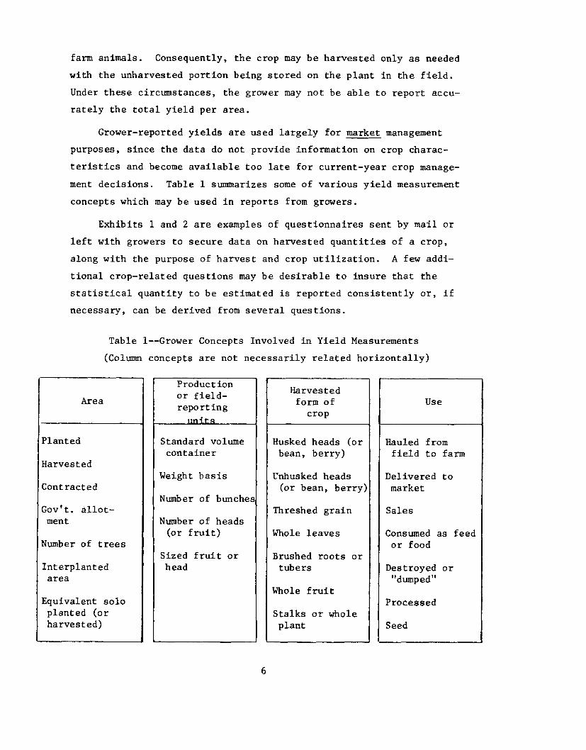
Grower-reported yields are used largely for market managementpurposes, since the data do not provide information on crop charac-teristics and become available too late for current-year crop manage-ment decisions. Table 1 summarizes some of various yield measurementconcepts which may be used in reports from growers.

Exhibits land 2 are examples of questionnaires sent by mail orleft with growers to secure data on harvested quantities of a crop,along with the purpose of harvest and crop utilization. A few addi-tional crop-related questions may be desirable to insure that thestatistical quantity to be estimated is reported consistently or, ifnecessary, can be derived from several questions.

Table l--Grower Concepts Involved in Yield Measurements(Column concepts are not necessarily related horizontally)

AreaProductionor £ield-reporting

l1T'lit-Q

Harvestedform of

cropUse

Planted

Harvested

Contracted

Gov't. allot-ment

Number of trees

Interplantedarea

Equivalent soloplanted (orharvested)

Standard volumecontainer

Weight basis

Number of bunches

Number of heads(or fruit)

Sized fruit orhead

6

Husked heads (or Hauled frombean, berry) field to farm

Unhusked heads Delivered to(or bean, berry) market

Threshed grain Sales

Whole leaves Consumed as feedor food

Brushed roots ortubers Destroyed or

"dumped"Whole fruit

ProcessedStalks or wholeplant Seed

EXHIBIT 1 - E~~PLE OF DATA COLLECTED FROM GROWERS ON GRAIN CROPS

ACREAGE AND PRODUCTION OF CROPS - 197

INSTRUCTIONS: Report for the land you are operating, including land rented from others.In reporting acres harvested and total production, include acres thatstill remain to be harvested and probable production.

REPORT FOR CROPS GROWN IN 197Give the information as accurately and completely as

possible. Where acreages and production are not definitelyknown, make careful estimates.

Totalproductionharvested

and to beharvested

FIELD CROPS

1. Corn planted for all purposes .

2. Corn harvested and to be harvested for grain .

3. Corn cut for silage .............•................................

4. Corn cut for fodder, pastured and hogged down (without husking) ..

5. Corn abandoned (will not be harvested or pastured) .

6. Soybeans planted for all purposes .

7. Soybeans harvested and to be harvested for beans .8. Sovbeans used for hay, silage, pasture only, plowed under or

abandoned .

9. Wheat planted for all purposes last fall and this spring .

LO. Wheat harvested for grain .Ll. Wheat used for hay, silage, pasture only, plowed under or

abandoned ..•.....................................................

12. Barley planted for all purposes last fall and this spring .

13. Barley harvested for grain .14. Barley used for hay, silage, pasture only, plowed under or

abandoned .

7

Bu.

EXHIBIT 2 - COMMON USES REPORTED FOR SOYBEAN CROP

SOYBEAN INQUIRYREPORT FOR THE FARM YOU OPERATE

1973 CROP PRODUCTION AND PURCHASES

1. oybeans HARVESTED for beanson this farm, last year's crop •.•....•• Bushels

2. IsoYbeans BOUGHT FOR SEEDI to plant the 1974 crop .....•••.....••.. Bushels

3. ITOTAL harvested and bought(sum of items 2 and 3) ...••••••....•... Bushe 1s

USE AND SALE OF ABOVE SOYBEANS

4. Soybeans SOLD AND TO BE SOLD betweenSept. 1, 1973 and Sept. 1, 1974 Bushels

s. Soybeans USED FOR SEED on this farmfor planting the 1974 cr,op Bushels

6. Soybeans FED AND TO BE FEDto livestock on this farm (beansfed whole or ground) betweenSept. 1, 1973 and Sept. 1, 1974...•..... Bushels

7. Old-crop soybeans expected to beon hand Sept. 1 this year .........•...•• Bushels

8. TOTAL (sum of items 4,5,6, and 7should equal item 8) •.......•........... Bushels

9. 1973- CROP SOYBEANS SOLD in eachof the following months:

Sold in 1973

September ..•.........•.•.....•••....• Bushe 1 s

8

AnswerhereJ,

1.3 Market- or Processor-Reported Production

For crops which are marketed or processed through commercialchannels, government or trade sources frequently report quantitieshandled monthly by elevators, gins, mills, oil processors, or crushers.Accurate data on the volume or weight delivered are available whenthe crop marketing is complete. While this is too late for eithercurrent-year market or crop management, the information is very use-ful in verifying the crop production, which serves as a basis foradjusting or revising crop acreage and/or yield estimates that areused in future yield forecasts and planning decisions.

The crop area harvested, in practically all cases, is estimatedfrom grower-reported data, or in some instances from land contractedfor specific crops by processing or marketing firms. In some cases,the acreage is based on production guidelines established by a govern-mental agency. Data on planted crop areas based on politically pre-scribed or suggested guidelines are usually unreliable. The yield isobtained preferably by dividing the market production by the grower-reported harvested acreage. The existence of these marketing datagenerally results in development of reliable yield data for historicalcrop series.

However, the yield concept is frequently altered, when these dataare used, to refer to reported marketed quantities rather than toamounts harvested by the farmer for all purposes. Such yield seriesmay be useful for determining marketed quantities, but may fall con-siderably short of measuring total quantities harvested. For cropsconsumed as food or feed without commercial processing this differ-ence can be important. For crops where utilization information fromfarmers can be obtained, it is possible to determine accurately thetotal yield harvested by combining the two sources of information.

The following table 2 presents some examples of the reporting ofquantities marketed or processed through government or trade sourcesin various countries.

9

Table 2--Some Crops Marketed or Processed(Column concepts are not necessarily related horizontally)

Crop

Cotton

Soybeans

Rice

Coffee

Oranges

Grapes

Cherries

Tobacco

Wheat

Sugar beets

Datasource

Gins

Crushers

Mills

Exporters

Gov't. inspec-tion andgrading

Wineries

Private pro-cessors totrade assoc.

Private auc-tions

Flour mills

Sugar facto-ries

Unitsreported

No. bales, grossor net weight

Oil, cake ormeal

Milled

Roasted

Juice, freshfruit

Tons crushedfor wine

Containerspacked

"Hands"

Milled

Tons of brushedroots, orsugar

Frequency

Monthly

For season

Seasonal

Semimonthly

Exhibits 3 and 4 are reports used by processors in reporting har-vested quantities of cotton and soybeans to a governmental agency.Exhibit 5 is a summary from weekly reports designed for state inspec-tors and graders of citrus. The individual weekly totals are accumulatedto give a running total for the season to date. This type of crop datais extremely valuable in checking the overall validity of yield andproduction models.

10

EXHIBIT 3: BALE WEIGHT REPORT OF COTTON GINNED PRIOR TO OCTOBER 1Crop of 1976

Total balesL. a • Total number of bales of cotton ginned from this crop •prior to October 1

Total weight

h. Total weight of the bales reported in item la above •• lbs •

c. The weight reported above is: [] NET (Excludes bagging and ties)

[] GROSS (Includes bagging and ties)

Average weight of ,baggingand ties used per bale

Z. Enter the AVERAGE weight of bagging and ties used per bale here_ lbs.3. If you are unable to report the total weight of bales ginned in item 1 above, please read the

following instructions and enter the necessary information in the columns below. Be sure tocheck above the column headings whether the weights reported for each bale are NET or GROSS.

a. If you ginned less than 1,000 b. If you ginned between 1,000 c. If you ginned ~ore thanbales: and 5,000 bales: 5,000 bales:

List each bale bearing tag List each b~le bearing tag List each bale bearingnumbers ending with 5 in numbers ending with 15, 35, tag numbers ending withcolumn (a) and enter bale 55, 75, and 95, in column 15 or 65 in column (a)weight in column (b). (a), and enter the bale and enter the bale

weight in column (b). weight in column (b).

The bale weights listed below are: 0 NET 0 GROSS

Bale Bale Bale Bale Bale Bale Bale Bale Bale BaleLine number weight number weight number weight number weight number weigh tNo. (Pounds) (Pounds) (Pounds) (Pounds) (Pounds)

(a) (b) (a) (b) (a) (b) (a) (b) (a) (b)1

2

3

4

5

6

7

11

EXHIBIT 4: SOYBEANS MONTHLY REPORT OF PRIMARY PROCESSORS

OItSEEDS, BEANS. AND NUTS

Report period - Mll'k UJith an "x" the box 1.Jhich January February March Aprilbest descl'ibes each l'epol'ting pel'iod -----.

1 Cal. Mo . 1 Cal. Mo. 1 Cal.Mo. 1 Cal.Mo.Product Item description Unit of Item 4 Weeks 4 Weeks 4 Weeks 4 Weekscode measure code

5 Weeks 5 Weeks 5 Weeks 5 WeeksSOYBEAN

0011611 Beans, crushed S. tons 0100

Crude oil produced2075111 (degummed weight) M. 1bs. 0105

2075113 Cake Animal feed S. 0111and tonsmealproducedfor - Edible pro-

2075115 tein products S. tons 0112

2075142 Lecithin produced S. tons 0114

2075261 Millfeed produced S. tons 0115

0011611 beans S. tons 0120

2075111 Stocks crude oil M. 1bs. 0125

2075211 cake and meal S. tons 0130

2075261 mi11feed S. tons 0135

12

EXHIBIT 5: FLORIDA WEEKLY REPORTS FOR CITRUS

PRELIMINARY WEEKLY PROGRESSIVE REPORT OF FRUIT RECEIVED AT PROCESSING PLANTSWeek Ending March 27 In units of 1-3/5 bu.)

Early-Mid Late Navel HoneyGrapefruit Oranges Oranges Oranges Tangerines Temples Tangelos K Early Tangerines Total435,359 188,110 616,710 140 13,296 3,220 9,193 1,266,028461,125 151,990 761,736 14,558 141 8,859 1,398,409345,970 75,391 651,119 5,275 279 5,280 1,083,374337,623 110,431 601,549 6,332 273 5,035 1,061,243489,835 106,828 732,804 6,281 4,134 1,339,882470,171 154,744 1,193,716 16,625 59 13,078 1,848,393

Total 2,540,083 787,494 4,557,634 140 62,367 3,972 45,579 7,997,329Previous

total 18,581,654 106,436,990 6,998,148 415,120 983,328 2,310,907 2,496,868 137,862 847 ,012 139,207,889GRAND TOTAL 21,121,737 107,224,484 11,555,782 415,260 983,328 2,373,274 2,500,840 137,862 892,591 147,205,218Correspond-ing totallast season 21,346,681 91,761,636 3,500,654 360,538 1,036,844 2,960,135 3,252,563 127,098 672,322 125,018,471

t-'W

Week Ending March 27 PRELIMINARY WEEKLY PROGRESSIVE REPORT OF FRUIT RECEIVED AT PACKING HOUSES In units of 4/5 bu.)Early-Mid Late Navel Honey

Grapefruit Oranges Oranges Oranges Tangerines Temples Tangelos K Early Tangerines Total121,175 575 63,287 654 21 5,992 191,704146,129 937 53,038 18 2,334 202,456209,078 370 45,705 1,159 1,515 257,827192,599 39,106 2,521 234,226190,282 54,831 777 7,345 253,235165,783 44 ,113 1,198 211,094

Total 1,025,046 1,882 300,080 2,608 21 20,905 1,350,542Previous

total 23,276,523 7,997,408 1,576,450 2,894,293 4,443,968 1,967,601 4,235,430 842,445 502,990 47,737,108GRAND TOTAL 24,301,569 7,999,290 1,876,530 2,894,293 4,443,968 1,970,209 4,235,451 842,445 523,895 49,087,650Correspond-ing totallast season 27,829,266 9,308,093 2,721,786 2,247,688 4,526,250 .4,221,881 4,158,512 438,453 2,076,323 57,528,252

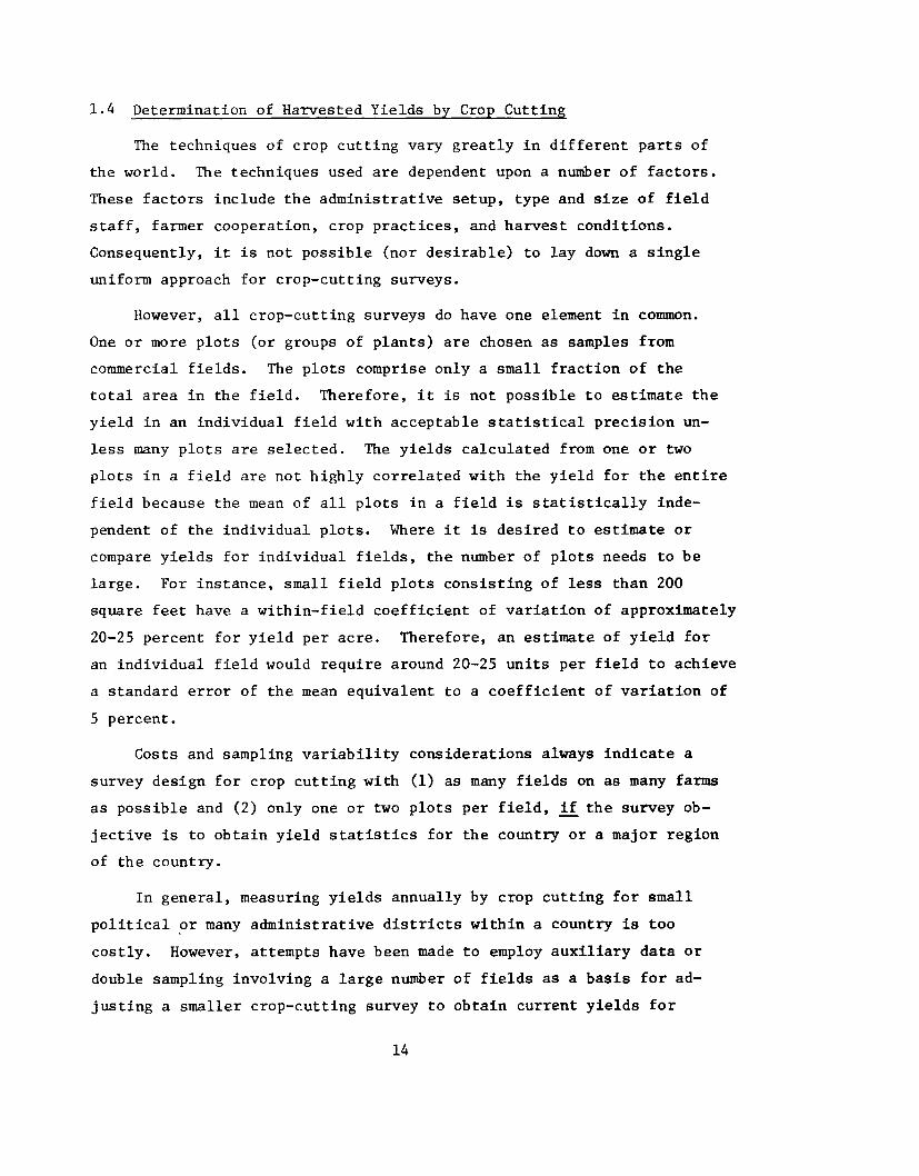
1.4 Determination of Harvested Yields by Crop Cutting

The techniques of crop cutting vary greatly in different parts ofthe world. The techniques used are dependent upon a number of factors.These factors include the administrative setup, type and size of fieldstaff, farmer cooperation, crop practices, and harvest conditions.Consequently, it is not possible (nor desirable) to lay down a singleuniform approach for crop-cutting surveys.

However, all crop-cutting surveys do have one element in common.One or more plots (or groups of plants) are chosen as samples fromcommercial fields. The plots comprise only a small fraction of thetotal area in the field. Therefore, it is not possible to estimate theyield in an individual field with acceptable statistical precision un-less many plots are selected. The yields calculated from one or twoplots in a field are not highly correlated with the yield for the entirefield because the mean of all plots in a field is statistically inde-pendent of the individual plots. Where it is desired to estimate orcompare yields for individual fields, the number of plots needs to belarge. For instance, small field plots consisting of less than 200square feet have a within-field coefficient of variation of approximately20-25 percent for yield per acre. Therefore, an estimate of yield foran individual field would require around 20-25 units per field to achievea standard error of the mean equivalent to a coefficient of variation of5 percent.

Costs and sampling variability considerations always indicate asurvey design for crop cutting with (1) as many fields on as many farmsas possible and (2) only one or two plots per field, if the survey ob-jective is to obtain yield statistics for the country or a major regionof the country.

In general, measuring yields annually by crop cutting for smallpolitical ~r many administrative districts within a country is toocostly. However, attempts have been made to employ auxiliary data ordouble sampling involving a large number of fields as a basis for ad-justing a smaller crop-cutting survey to obtain current yields for

14

small geographic regions. The auxiliary data needs to be acquired quitecheaply and to be highly correlated with the yield from the crop-cuttingplots. Typically, eye estimates of yield per acre are made for manyfields (or trees) and a random subsample of fields for crop cutting istaken. Under favorable costs and moderate-to-high correlation betweenthe two data sources, annual crop-cutting surveys can provide yieldstatistics for small areas. However, the number of instances wherethese techniques have been successfully employed for small-area yieldstatistics is very small, because costs and correlations of the two datasources have not been favorable.

Yield measurement by crop cutting has been largely confined to majorfood or export crops in India, Europe, and the United States. In theUnited States, industry marketing programs for specialty fruit and nutcrops have employed crop-cutting techniques for yield information.

1.4.1 Sample SelectionThe measurement of yields by crop cutting involves the selec-

tion of a representative (probability) sample of fields or blocksof trees. The process of plot selection within the field alsorequires very careful location, measurement of plot size, delin-eation of the plants associated with the plot as well as carefulhandling of the plant parts that are used to derive the yield perarea. The following table illustrates the major steps requiredin the selection process for a field crop.

15

Table 3(a)--Sample Field and Plot Selection

Selection Step Information Needed

1. Random selection of farms List of farms having crop for whichyield is to be estimated

2. Random selection of Number of fields or area of each tofields determine probabilities of selection

for individual fields

3. Subdivision of field Dimensions of field or number ofinto plots crop rows in field, used to deter-

mine plots of a given size and shape

4. Random selection of Identification of randomly selectedplots fixed-size plots to be measured or

marked off by a preconstructed frame

5. Selection of certain An enumeration of all the plantplant parts for measure- parts (normally the basic yieldment components)

6. Selection of some plant Weight or other measure of heads orparts for cutting other plant parts

7. Selection of grain to be Determination of grain fraction,forwarded for laboratory moisture and, in some cases,analysis quality factors

8. Selection of plants and Number of heads and weight of grainarea to be gleaned after attached to heads as well as loosecommercial or normal grains on ground missed or lost fromharvest procedure harvesting equipment

16

A corresponding table for a tree crop would be as follows:

Table 3(b)--Sample Block and Tree-Part Selectionfor Data Collection

Selection Step Information Needed

1. Random selection of farms List of farms or commercial plant-ings with tree crop

2. Random selection of Number of trees, age, variety forblocks of trees all blocks for deriving probabili-

ties for selecting individual blocks

Rows of trees and trees per row are3. Random selection of trees used to determine selection proba-

bili ties

4. A random selection of a The main trunk and primary-limbsmall portion of tree isto be made since complete sizes and number, as basis forharvesting is costly selection probabilities

5. Terminal limb selection Identification of terminal limbs(and possibly paths to from which to count fruitlimbs)

6. Random selection of fruitor clusters to be removed Weight and/or size of fruit removedfrom tree

7. Random selection of fruit Ratio of fruit ''berry''or nut "meat""berry" or nut "meat" atspecial field stations weight to total fruit weight

8. Random selection of trees Number of fruit and weight ofand ground area to be berries on trees and ground missedgleaned after commercial or lost in harvestingharvest

17

1.4.2 Plot Size and Location

Variations in plot size are primarily dependent upon costsand the magnitude of variance components between and withinfields. In some countries the ability of the workers to layout and harvest plant materials in plots according to specifi-cations is an additional factor which is considered in choosingthe plot size. The smallest plot sizes for field crops are usedin the U.S. where an area as small as 0.0001 acre (approximately)has been used. Much larger plot sizes are found in India whereplot sizes as large as 0.1 acre have been used.

Table 4 gives some examples of plot sizes and shapes whichhave been used throughout the world. Table 5 lists some of thecrops in various countries where crop-cutting surveys have beenemployed. Neither table is complete, but they do suggest thewide application of this technique.

18

Table 4--Size and Shape of Plots Used for Field Crops

Plot size

2, 4, 5, 8 ft diameter3 meters diameter5 ft 3 in. (1/2000 acre)33 ft x l6~ ft (1/80 acre)

(50 x 25 (links»l6~ ft x l6~ ft (1/160 acre)33 x 16 (1/80 acre)5 x 10 meters1.5 sq meters.3 sq meter15 ft x 2 rows7 x 7 yd (1/100 acre)6 ft 7 in. (1/1000 acre)33 ft16 ft 6 in.8 ft 3 in.24 in. x 26.136 in. (1/10,000

acre)21.6 in. x 3 rows1 sq meter

Entire field

19

Shape

CircularCircularCircularRectangular

RectangularRectangularRectangularRectangularRectangularRectangularSquareSquareTriangular (Equilateral)Triangular (Equilateral)Triangular (Equilateral)U-shaped frame

Length-af-row frameSquare frame with closingbarIn terraced areas wherevery small parcels areseeded

Table 5--Crop-Cutting Surveys by Countries

Crop Country

Wheat India, U.S., W. GermanyRice IndiaCotton India, U.S.Sugarcane IndiaCoconuts IndiaAlmonds U.S.Walnuts U.S.Citrus U.S.Peaches U.S.Pears U.S.Lemons U.S.Grapes U.S.Cherries U.S.Cranberries U.S.Soybeans U.S.Tobacco U.S.Corn U.S., BasutolandSorghum U.S., BasutolandPeas BasutolandBarley BasutolandOats BasutolandBeans BasutolandRye W. GermanyPotatoes W. Germany, U.S.

20

CHAPTER 2 - MODELS FOR FORECASTING YIELDS BASED ON PLANT RESPONSE

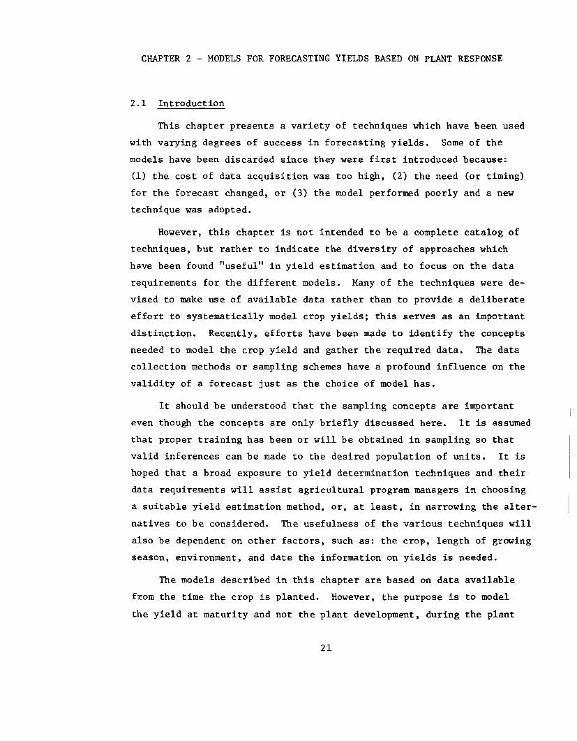
2.1 Introduction

This chapter presents a variety of techniques which have been usedwith varying degrees of success in forecasting yields. Some of themodels have been discarded since they were first introduced because:(1) the cost of data acquisition was too high, (2) the need (or timing)for the forecast changed, or (3) the model performed poorly and a newtechnique was adopted.

However, this chapter is not intended to be a complete catalog oftechniques, but rather to indicate the diversity of approaches whichhave been found "useful" in yield estimation and to focus on the datarequirements for the different models. Many of the techniques were de-vised to make use of available data rather than to provide a deliberateeffort to systematically model crop yields; this serves as an importantdistinction. Recently, efforts have been made to identify the conceptsneeded to model the crop yield and gather the required data. The datacollection methods or sampling schemes have a profound influence on thevalidity of a forecast just as the choice of model has.

It should be understood that the sampling concepts are importanteven though the concepts are only briefly discussed here. It is assumedthat proper training has been or will be obtained in sampling so thatvalid inferences can be made to the desired population of units. It ishoped that a broad exposure to yield determination techniques and theirdata requirements will assist agricultural program managers in choosinga suitable yield estimation method, or, at least, in narrowing the alter-natives to be considered. The usefulness of the various techniques willalso be dependent on other factors, such as: the crop, length of growingseason, environment, and date the information on yields is needed.

The models described in this chapter are based on data availablefrom the time the crop is planted. However, the purpose is to modelthe yield at maturity and not the plant development, during the plant

21

life unless this is necessary to model the yield at maturity. Severaldifferent models are discussed in sufficient detail so the reader willbe able to grasp the data collection and modeling concepts.

In some cases, the examples cited may provide a basis for startingnew work on the same or similar crops. An acreage inventory survey isassumed to have been completed after planting so sample farms or fieldsmay be selected for observation. Likewise, the acreage sample is ex-pected to provide validation of harvested yields or yield componentsas well as permit the derivation of production based on yield andacreage. Most of the models presented were developed on a farm, field,plot, or plant basis. For some yield models, especially those involvinga historical series of data, averages derived from several discretelocations are attributed to large geographic areas rather than indi-vidual fields or plots.

Grower observations on reporting units are generally in terms ofyield per harvested area for either the farm or individual fields. Insome instances, public-minded growers may be willing to cooperate byobserving plots or plants for governmental or industrial organizations.Models using plant counts and yield-component-measurement techniqueswhich are carried out by volunteer or paid cooperators usually are ona plot or plant basis. The models based on plot or individual plantdata are expressed in terms of a standard unit for conversion to a peracre or per hectare basis by the sponsoring agency for publication.

22

2.2 Mathematical ModelsThe choice of model is a basic forecasting step. In general, the

techniques commonly used do not consider the data as a time series fromwhich forecasts are made, but as a series of independent data pointswhere a new observation(s) is generated each year; neither is it likelythat purely mathematical rules can be found which will be adequate todescribe the phenomena.

The models rarely describe the real world, owing to random ornatural variation shown by most data from commercial crop plantings andplots. Thus, the forecasting methods that have been developed areeither statistical in nature or require statistical estimates of keyparameters for successful implementation. Some of the models aredeterministic, but these generally require statistical estimates ofsome of the model parameters for implementation in large areas. Inaddition, the models are generally incomplete because some importantfactor has been omitted due to either our incomplete understanding ofthe phenomena or the cost of including it in the model. Often we usethe models, not in the belief that they describe exactly the underlyingstructure of the situation, but in the faith that, at least for therecent past and the near future, they give a reasonable description ofthe underlying situation.

We consider several situations. In the first situation, the struc-ture is regarded as highly stable over years and the chosen modelrepresents the underlying structure of the data. The model in thiscase will be referred to as a between-year or global model.

In the second situation, the structure is believed to be stable inthe short run but not necessarily in the long run. Slow changes in themodel structure or parameter values may occur which will not affect thedata adversely enough to invalidate the forecast for only one year ahead(or a short period). In this case, the model will be referred to as atransitory or local model.

23

In a third situation, the structure may be unstable over the shortrun. The model in this situation is referred to as a within-year orindividual crop-year model.

Experience suggests that using transitory models often leads tobetter forecasts, because we have many more replications in time forevaluation of the method, while the between-year or global model may beviewed as a single observation of the process or phenomenon. The within-year or individual crop year phenomenon is recognized, but too oftenthere are little data available to model the situation. Frequently,there is no difference in the mathematical or statistical formulationof these models, but the differences lie in the way in which we make useof or interpret the parameters represented in the models.

Several basic statistical models are described before examiningtechniques which have been developed and put in use. The simpleststatistical model is the constant-mean model:

x = ~ + Et t

where x = past data for the tth period (usually years) fort

a yield characteristic xl' x2' •.., Xt

E = the normal random error for time tt

~ = a constant mean

and we wish to forecast the characteristic for time t+k.

The forecast for time t+k is given by the sample mean

The model might be appropriate for weight of grain per head, or weightof grain per kernel where x is for a series of years; that is, an over-

tyears model might be appropriate for certain characteristics of theplant even though it might not be appropriate for yield per area.

24

Another formula for the constant mean which might be used when atransitory model is appropriate is that which assigns weights to thedata points as follows (for computation of coefficients see page 102):

- 2xt+k = (l-a)(xt + a xt_l + a xt_2 + ...)

where "a" is a number between 0 and 1. Typical values of "a" for yieldwork would be between 1/3 and 2/3. This model has the effect of alwaysgiving the greatest weight (or importance) to the last observed datapoint. The above formula can be rewritten so it is more convenient touse for calculation purposes, as

x = (l-a)x + a xt+k t t-l,k

This is a type of moving average, but gives variable weights to theyears, in contrast to the simple moving average, which gives an equalweight to each year. Again, this model might be appropriate for cer-tain plant characteristics or yield per area.

Where neither a between-year nor transitory model is appropriate,a within-year or logistic-type growth model may represent the dataapproximately:

where xt given data value for time t in a sequence of timesduring crop season for a yield characteristic

a,8,p, = constants or model parameters

£ = random error for time tt

and we wish to forecast the characteristic for time t+k.

Some of the other models commonly encountered are as follows:

Xt = a + 8t

Linear regression: Xt = a + 8Zt where Zt is another variable.

Linear trend: for all t (i.e., the time variable).

25

Autoregression: xt

a + Bx 1 where x 1 is the previous valuet- t-

of x.

Exponential growth: Xt BtaE: fo r all t.

First-order movingaverage: x = E - BE:t t t-l where e is a constant between

-1 and 1.

The linear-trend model to be employed can be either global or local.The ideas are similar to those in the constant-mean model in that theleast squares line can be altered by assigning different weights (orimportance) to the errors to be minimized in estimating the modelparameters. This has the effect of forcing the trend line to fit themost recent data points more closely. Similar ideas, likewise, carryover to the linear-regression model; however, the regression model alsorequires attention to the selection of the other variable. In most ofthe models the forecast time is t+l, except for the growth model, wheret+k is "quite large" compared with t.

During the past few years, a major emphasis has been given to de-veloping yield models in which the parameters are derived from thecurrent year for use prior to harvest. That is, a deliberate efforthas been made to make the techniques less dependent on a historicalseries of data as a prerequisite to being able to forecast the yield.Models that achieve this independence are referred to as "within-yearmodels" and are considered to be more desirable than between-year modelsif each year is different from the preceding years or there are tech-nological changes taking place which cannot be evaluated. The fact thatthese models do not require a historical series of similar informationbefore yield forecasts can be started is considered quite important whenstarting work on a new crop or developing a system for a country withouta crop-forecasting system.

However, the models which do not depend on historical series ofyields require greater understanding of the relations of plant responsesor growers' knowledge of harvested yields. This type of model has been

26

considered for yield forecasts based on both grower subjective yieldforecasts or appraisals as well as objective yield methods. It is help-ful to start with a look at grower yield appraisals (or probable yields),which are used for many crops.

The fact that relatively few crops have been included in yieldforecasting, based on plant characteristic or crop-cutting programs forcountries with official published series, suggests that this approachshould be examined carefully. In addition, opportunities for use ofgrower appraisals exist in technical assistance work when startingcurrent statistical programs in crop-yield and crop-production fore-casting.

The remainder of this chapter is devoted to a discussion of varioustechniques which have been tried. In general, no attempt has been madeto evaluate each method or compare it with all competing models, sincethe necessary information for doing this was not available. However,it is hoped that by the end of the manual the reader will recognize someof the differences in the model assumptions, data needs, and the abilityto validate the forecasts and model parameters as factors to take intoconsideration when comparing forecast models.

27

2.3 Grower Subjective Appraisal Systems

A common approach used by governmental agencies and private fore-casters is the charting or deriving of relations between grower forecastsof probable yields and harvested yields obtained at the end of the sea-son. This approach is based on the relations over years. being the samefor a period of 5-10 years. but is frequently put in use after yieldshave been collected for only 3-5 years. In most cases. yield charts orrelationships are based on voluntary reports from growers or cooperativeagents who report by mail. telephone. radio. or messenger. Consequently.the reported probable yields frequently may not be representative of thepopulation and/or the reporters may not be able to forecast the cropaccurately for their village. district, region. or some area withvaguely defined boundaries. In either case, the probable yields requireadjustment or correction for various kinds of unknown biases. Frequently.there appear to be different relations indicated for different periodsof years. The dashed lines in Figure 1 indicate approximately the natureof two different regressions, and the solid line the least squares re-gression line over both periods. This chart illustrates some of thecommon problems associated with between-year or global regression lines.There may be a strong trend and neither the representativeness of thesample nor the ability of the growers to forecast their yields is mea-sured or known. The same information is frequently analyzed by employinga time trend chart and plotting the residuals or deviations from theforecasted yields against time.

Table 6 indicates the correlation and nature of the linear relationbetween growers' forecasts and their reported harvested yields for sev-eral crops. The relations found for cotton and soybeans in both yearsin adjoining States are similar. but the relations for corn are differ-ent in each of the years in adjoining States. In general, the rangesin the average yields over years based on probability surveys of growersand crop-cutting surveys agree closely. but the levels of the growers'average yield are several percent lower.

28

FIGURE 1 - CORN HARVESTED YIELD VS. GROWER PROBABLE55 YIELD - AUGUST 1

195<) - 19737~~

67/50 /

/45 ~6/.71

/ 70

40 / 59-65~ ~9 /"< 61t"1

/tfl /...,t"1 YN 0 35\0 ...:: 66-73H

63 ,/t"1b

/59 6430

60 62

25

5550454035302520

20

GROWER PROBABLE YIELD

INDIVIDUAL YEAR DATAREGRESSION LINE FOR YEARGROUPINGSREGRESSION LINE FOR ALL YEARS

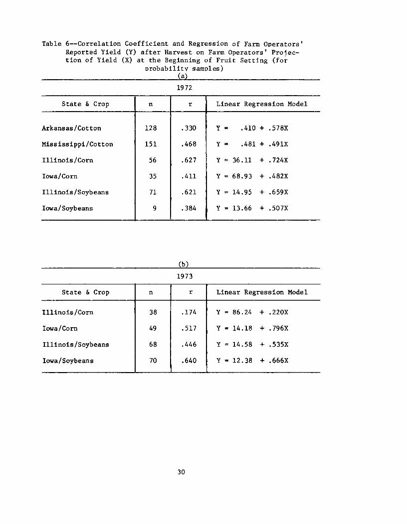
Table 6--Correlation Coefficient and Regression of Farm Operators'Reported Yield (Y) after Harvest on Farm Operators' Projec-tion of Yield (X) at the Beginning of Fruit Setting (for

probability samples)(a)

1972

State & Crop n r Linear Regression Model

Arkansas/Cotton 128 .330 Y = .410 + .578X

Mississippi/Cotton 151 .468 Y = .481 + .491X

1111nois/Corn 56 .627 Y = 36 .11 + .724X

Iowa/Corn 35 .411 Y = 68.93 + .482X

Illinois/Soybeans 71 .621 Y = 14.95 + .659X

Iowa/Soybeans 9 .384 Y = 13 •66 + .507X

(b)

1973

State & Crop n r Linear Regression Model

Illinois/Corn 38 .174 Y = 86.24 + .220X

Iowa/Corn 49 .517 Y = 14.18 + .796X

Illinois/Soybeans 68 .446 Y = 14.58 + .535X

Iowa/Soybeans 70 .640 Y = 12.38 + .666X

30

Sometimes a different approach is needed to overcome shortcomingsdue to trend, changing relations over time, or even the influence ofprevious crops on the current year's appraisal. An approach will bediscussed which provides at least partial answers to some of theseproblems. The method is referred to as the "grower-graded yieldappraisal." It seeks to determine the following: (1) What does thegrower expect the yield of a specific planting of a crop to be?(2) How does the grower rate (or evaluate) the expected yield of thisplanting of the crop according to five descriptive categories? Theacreages (or areas) planted are then summarized by the five categoriesand the average or expected yield (or expected production) is derivedby weighting the yields with the acreages or percent of acreages re-ported by categories.

The descriptive ratings provided by the growers are assumed to bedistributed normally, as in the grading system commonly used by teacherswhen a large number of students are to be graded. Thus, the name"grower-graded yield appraisal" is given to the method, since thegrower, in effect, "grades" his own yield appraisal. This gradingscheme and its relation to the normal distribution is illustrated byChart 1 on page 33.

Some experience with this approach in Central America has indicatedthat the growers do grade their yields in approximately this manner.That is, 40-50 percent of the acreage is reported by growers early incrop season to have an expected yield which is "average." The remainingexpected yields are either one category above or below the average.These results suggest most growers report an average yield early in thecrop season. The interpretation of the expected yield as prophesizingthe harvested yield may be in serious error in any year that is notaverage or normal. Stated another way, many growers may not be skill-ful forecasters or do not wish to forecast a yield different from theaverage for purposes of reporting to public agencies. The most usefulinformation comes from those growers who report a yield which is notaverage.

31

The procedure for reporting yield prospects to user agencies,private or public, for the coming harvest is as follows: (1) Fromland use surveys, the estimated acreage is summarized as the percentof acreage reported for the grade categories used; (2) The growers areasked to report their expected yield; and (3) The within-year averageyield in (2) is derived from the categories by the percentage of theacreage in (1). The rationale behind this approach is that it may bedesirable to provide the grower's expected yield, the descriptiveappraisals, and the derived within-year average yield so that theusers may review this data along with other information that theymay have from other sources and years. Expected production can alsobe reported to the user in place of yield if this is preferable. If thewithin-year derived average yield differs from the grower's last year'saverage yield (or a five-year average), the user is aware of this dif-ference and may wish to place a somewhat different interpretation orevaluation on crop prospects.

For application to specific crops, the normal distribution may beskewed slightly if a portion of the crop is grown on either dry1and orirrigated land (this may be handled by altering the tail probabilitiesand X-scale values of the model). When a large fraction is grown onboth irrigated land and dry1and, a separate yield forecast should bemade for the acreage of each. In the Dominican Republic, coffee andrice are expected to have crop failures less frequently, and outstand-ing crops more frequently, than shown in Chart 1. This is the resultof increased management inputs, established trees or areas in the caseof coffee, and availability of water for rice. Consequently, the prob-ability in the right-hand tail was increased. In contrast, corn andbeans are two crops which would be expected to have their distributionsskewed in an opposite manner from coffee and rice.

32

Chart 1: Grower-Graded-Yield-Appraisal Curve for a Large Number of Fields

Below Above MuchPossible Crop Average abovefailure average averagecrop averagedescrip- Very Poor Normal Good Very

tion poor crop crop crop goodcorres- crop crop

ponding No Outstandingto grades harvest ExcellentStandardized

Grade Scale

(uniform) o

F

.4

D

.8

C

1.2

B

1.6

A

2.0yield scale

Midpoint of .2 .6 1.0 1.4 1.8interval Xi

The range of the yield scale is 0 to 2.0 and each of the 5 grades coversone-fifth of the X axis (uniform scale).

5E(X) = E PiXi = 1.00 (average yield)

1

Alternative scaie values developed for use in the Dominican Republic were basedon the approximate center of the probability assigned to the interval ratherthan on a uniform X scale. The me~its of alternative scales to the uniformscale have not been fully verified but the ones proposed have ~iven accept-able results.

Center ofprobability in .08 .32 1.00 1.68 1.92interval Zi

33

2.4 Crop-Weather Relations for Predicting Yields

2.4.1 Introduction

Crop-weather relations have been studied by many investigatorsas a means of forecasting crop yields. This approach is based onthe premise that a network of weather stations has been recordingtemperature and precipitation for a number of years and data onharvested yields are available for the same period. In most cases,the yields have no known measure of accuracy available, and thetechnique is largely heuristic.

In some instances the network of weather stations coincideswith important regional population centers rather than being dis-tributed geographically to coincide with the crop acreage. Underthese circumstances, the crop-weather relations may be distortedand not well suited to forecasting of individual crops, unless theweather variables are rather uniform over broad areas so that aspecial network of stations providing paired observations is notneeded. The utility of these techniques depends on the climatebeing critical at one or more phenological stages of the crop forthe area or country. Many of the applications of this techniqueinvolve crops which also have marked technological trends thatexplain a portion of the year-to-year variations in yields, whilethe weather variables account for departures from expected yields.Generally, little or no phenological information on the crop isavailable.

2.4.2 Joint Precipitation and Temperature Effects

One of the problems in crop-weather research is that ofmeasuring the joint effect of various weather factors simultaneous-ly. For example, the effect of an inch of rain on the final yieldof a crop depends to a large extent on the temperature and otherweather factors associated with that rainfall during a criticalstage of development.

34

One part of a crop-weather project in the U.S. was the attemptby Hendricks and Scholl to develop approaches to measuring thejoint effects of several weather factors. The method involved theuse of monthly temperature and precipitation data as an indicatorof the departure of the yield of corn from the expected yield.The use of monthly averages may be unsatisfactory without a modelparameter or factor which incorporates the occurrence of unusualshort-duration events of the variables having a critical impact onyield. In these cases, the error term in the model will drasticallyunderstate the expected error. Modification of the model valuesfor the weather variable must frequently be based on special con-trolled experiments, since these phenomena occur infrequently andtheir effects on yield are difficult to measure quantitatively.The parameters should provide for modification by an event multi-plier such as E = (1 + 0)n, where 101«1 (i.e., much less than 1)is the effect of a single occurrence of the event and n is thenumber of times the event occurs in the month or period averaged.Generally, the event E is assumed to occur infrequently over yearsand only once or twice a period, so that n is a small integer.In general, the occurrences of unfavorable events are better known,because the critical growth stages occur early in the developmentof the crop and the events are better reported by the press andagricultural industry.

The charts (pages 38-41) for the State of Illinois illustratethe techniques developed in 1951 by Scholl and Huddleston for anarea where the climatic factors are generally not critical buttechnology is important. Following is a brief description of howthe method was developed. The method was first used in graphicform, but later was expressed in equations.

The first step is that of computing the lO-year movingaverages (other periods could have been used) of corn yields(Chart 2) to eliminate the effects of all nonweather factors(1.e., "technology") on yields so that the net effects of weather

35

could be better evaluated. Obviously, one disadvantage of using10-year averages is the necessity of projecting the trend ornormal yield so that it may be used currently for forecasting.

The next step involves constructing the isograms on a chartfor each month during the critical period of crop growth (June,July and August). These charts are prepared by plotting themonthly rainfall (i.e., daily precipitation accumulated for themonth) data on the X axis, and temperature values (i.e., dailymean temperatures averaged) on the Y axis. The departures of thefinal annual yields from the 10-year moving average were insertedat these points. For example, assume a monthly temperature of75 degrees and rainfall of 3.00 inches for one of the June monthsin the series; also, assume a departure of yield from the trendline of +5.0 bushels for this particular year. The line coin-ciding with 3 inches of rainfall on the horizontal scale of theJune Weather Chart (No.3) is followed up until it intersects theline coinciding with 75 degrees on the vertical scale. At thispoint the figure +5.0 is entered. This is repeated for each Junein the series of years. Isograms which best represent equaldeparture values of yields are then drawn on the chart. Obviously,judgment or subjectivity is involved in drawing these lines. Iteven may be necessary to ignore partially some of the individualdata points in drawing the isograms. A period of 40 years wasused in the study.

In drawing these isograms it is assumed that the most radicaldepartures in final yields are the accumulated results of weatherduring several months, since a crop failure has never been experi-enced in any major geographic area of Illinois. Therefore, thefull amount of such departures should not be allowed for in anyindividual month. It appears that perhaps no ~ than half theextreme departures should be indicated by the isograms for anindividual month. For example, the isograms on the July chartmight indicate a range from -6 to +6 bushels; whereas, the actualdepartures for some individual years are considerably larger.

36

The same types of joint relations between rainfall, temperature,and yields were also investigated more rigorously through mathemat-ical models, such as:

y a + bT + cR + d(TR) (1)

or y = a + bT + cR + d(TR) + gT2 + hR2 (2)

where T average monthly temperatureR = monthly rainfall

and a, b, c, d, g, and h are regression parameters.

The individual monthly charts giving the estimated joint effectsof temperature and rainfall, after removal of trend, are shown asCharts 3, 4, and 5 for equation (1). These charts were generated bya computer plotter.

In order to limit the effects on yields attributable to anindividual month, the departures from the mean yield for each monthmight be divided by two or three, as was done for the graphic approach.This is equivalent to dividing the calculated slope parameters (b, c,g, h) for a month by 2 or 3 in the alternative form of the regressionequation (1).

yt

y + ~ (Tt - T) + ~ (Rt - R) + ~ (TR - TR) (3)

where y = is the normal yield based on trend (or base-periodaverage yield if no trend is present)

T, R, and TR are the averages for the base period

Tt' Rt' and TR are the monthly values for year t .

An alternative way of adjusting the slope parameters for a monthis to multiply by the correlation coefficient squared, R:, divided by

1

3L R: , where R2 is the multiple-correlation coefficient squared for

i=l 1 i

an individual month. However, June and July were the key months.The relation for August was the least important, since after corntasseling in July the plant is fully developed and soil moisture isless important.

37

CHART 2 - ILLINOIS CORN - TE:~-YEAR SIMPLE MOVING

AVERAGES OF YIELD ?ER ACRE

90

80

70

600<Hrrt

bw "d00 rrt 50llll

>nllll~

45

40

35

1910 1915 1920 1925 1930 1935 1940 1945 1950 1960 1970

CHART 3 - YIELD DEPARTURE ISOGRAMS BASED ON JUNE RAINFALL AND TEMPERATURE

REGRESSION EQUATION: Y' = 173.801-43.275R-2.475T+O.6208RT

:JII

Lf1J0)1I

i01

0,1, ,!

f6lI

Lf1~

:jI

Lf1...,.\----.-, ----~I ----I ------r----.--.----,-="0.0 2.0 4.0 6.0 8.0 10.0 12.0RAINFALL (INCHES)

39

CHART 4 - YIELD DEPARTURE ISOGRAMS BASED ON JULY RAINFALL AND TEMPERATURE

REGRESSION EQUATION: Y' = 89.939-21.nnR-l.2h3T+O.3397RTL()a

~L-~~,u. I I I I

~O.O 2.0 4.0 6.0 8.0 10.0 12.0RAINFALL (INCHES)40

,

:ST'~~T~~ + -12 I

x -10

~: I-4-2

o24

6

810

12 :....J

:r

I!J

ot.D

oo

~1~l

~~~•..... IlL::r: iz~0:::0~co~v:.~

I~

\p:::c;.n~f'

Lc::

~0:::;:::;E-<o;;:if'~p...::;::;~E-<

'J)(D

CHART 5 - YIELD DEPARTURE ISOGRAMS BASED ON AUGUST RAINFALL AND TEMPERATURE

REGRESSION EQUATION: Y' = 114.710-16.328R-l.559T+O.2261RT

If)0-••.• 1

I

y

)(

z

•

L£GE.N[J ,

"""-, T' I

I ~ I :1n-4 !

I

-2 Io I

2

468

10

12 I

J

J....---~I---~I---~I----I----I-----'~O.O 2.0 4.0 6.0 8.0 10.0 12.0RAINFALL (INCHES)

4]

2.4.3 Agrometeorological Forecasting of Crop Yields

In the USSR great attention has been paid to the scientificinvestigations aimed at finding the relations between the pro-ductivity of basic crops and the agrometeorological conditions.Methods have been developed by Ulanova and other workers for theagrometeorological forecasting of crop yields and the preparationof outlook guidance for the yields of crops. The relations dis-covered between the cereal crop productivity and agrometeorologicalconditions also are used to divide the territory of a state or en-tire country into agrometeorological areas in estimating the extentof favorable climatic resources for the growth of a crop. Relationshave been found for the basic cereal crops, spring and winter wheat,as well as for corn.

Quantitative relations have been found between the yield ofwinter wheat and the soil water storage in spring. It was foundthat the main inertial factors for the future winter-wheat yieldin the black-earth zone are the water storage in the upper one-meter layer of the soil and the number of stems of winter wheat persquare meter in the spring. Summer precipitation is of less impor-tance, and the dependence of the winter-wheat yield on the summerprecipitation (without taking into account the soil moisture andwinter-wheat state) is low.

The temperature during the spring-summer period in the black-earth regions of the USSR is completely sufficient (i.e., notcritical) for the winter wheat.

The analysis of a long series of data shows that, althoughwinter-wheat yields in the Ukraine and the North Caucasus dependmainly on spring water storage during many years, a good forecast-ing relation between crop yields and spring water storage can befound by taking into account the number of stems that survivedthe winter.

42

It is known that the number of stems of the winter wheat duringthe period of spring-summer vegetation does not remain constant, butthe number of stems in spring may be considered as an indicator ofthe probable number of eared stems in the future.

As a result of field observations of winter wheat carried outby hydrometeorological and agrometeorological stations, a ratherclose relation between the number of eared stems of waxen ripeness(mature heads) (Y) and the number of stems in spring (X) of thedifferent kinds of winter wheat was found.

For the winter wheat of Belotserkovskaya 198 kind (i.e., vari-ety), the equation of the relation is:

Y = 0.22X + 199.0 r = 0.75

And for the winter wheat of Bezostaya 1 kind

Y = 0.24X + 241.2 r = 0.79

In winter wheat of Odesskaya varieties 3, 12 and 16, thequantitative relations between spring-effective soil moisturesupply and the number of stems in spring are given below for high-quality agrotechniques on the same fallow in black soils of steppeand forest-steppe zones of the Ukraine and the North Caucasus.

The equations are given for most probable crop yields (Y) tobe expected and also for the highest (Yh) and the lowest (YL) yieldsthat are predicted from the soil moisture (X) in millimeters in thetop meter of soil during April, May, and June.

The regression equations of winter-wheat yield on springmoisture supply in years of favorable autumn-winter conditionswhen the number of stems of winter wheat in spring was 1,000 to2,000 per square meter, have the following outlook:

(a) lowest crop yields (YL) under unfavorable weather con-ditions of April, May, and June:

YL = 0.24X - 16.0

43

(b) highest yields (Yh) under the most favorable weatherconditions of April, May, and June:

Yh = 0.24x - 4.4

(c) the most probable winter-wheat yields (Y) in a particularyear:

Y = 0.24X - 10.2

The coefficient of correlation of this relation is r = 0.86. Anerror of the equation of regression is S = + 3.4 centner/ha.

y

The relation of winter-wheat yield of Odesskaya 3, 12, and16 to spring supply of moisture in years of unfavorable autumn orwinter conditions with a small number of stems in spring (400-900per square meter) is presented by the following equations:

(a) the lowest yields (YL) under unfavorable conditions ofweather of April, May, and June are as follows:

YL = 0.2X - 15.0

(b) the highest yields (Yh) under the most favorable weatherconditions of April, May, and June have an outlook:

Yh = O.2X - 7.2

(c) the most probable expected yields (Y) have the outlook:

Y 0.2X - 11.1

The coefficient of correlation is r = 0.89. An error of theequation of regression is S

yequations X is the productive moisture supply (mrn) under winter

+ 2.9 centner/ha. In the

wheat in a one-meter soil layer at a mean daily air temperatureof +5° in the spring, where all the equations act in the rangeof the values of spring moisture supply from 100 to 200 mm. Thetechnique is based on forecasting yield from the soil water duringApril, May, and June after "conditioning" yield on the expectednumber of stems per square meter.

44

2.4.4 Auxiliary Environmental Variables and Yields

Variables such as hourly or daily temperature, rainfall, solarradiation, minutes of sunshine, dew point, and others are used toderive new parameters directly identifiable with plant growthprocesses. The physical and physiological variables which arecommonly derived are photosynthesis, available soil water, evapora-tion-transpiration, light interception, albedo, and canopy tempera-ture. While it would be possible to measure some of these variablesdirectly, the cost of instrumentation and data collection for anextensive network of locations is beyond the normal budgetary meansof most users of crop yield data. Consequently, most of thesevariables are estimated or approximated through relations withweather data normally collected by an established experimentstation or meteorological network. However, these networks aregenerally too sparse or the location of equipment is not representa-tive of the plant environment for a widely dispersed commercial crop.These two factors introduce errors into the "independent" or pre-dictor variables which lead to bias in the estimated parameters inthe model, as mentioned earlier.

The idea of relating crop yields to derived variables such asevapotranspiration is not new. One model is presented, but therehave been many attempts during this century to employ evapotrans-piration. The basic assumptions are that (1) water is the majorlimiting factor in most crop production situations and (2) astranspiration is decreased by water stress, photosynthesis isproportionally decreased and thus affects yield. Hence, pertinenttranspiration relations should reflect relative photosynthateproduction (yield).

A versatile and effective ET model has been described byKanemasu. This model has been adapted and tested for winter wheatacross Kansas with some success, and applied to soybeans with betterresults. The yield (actual) and ET model data were available forseveral sites for the crop years 1974-75 and 1975-76. Selected

45

sites were used as calibration points, and regression analyses ofvarious model formulations for yield prediction were evaluated.Wheat yield differences were related to the number of days in eachgrowth stage--the greater yields occurring in lengthened seasons.

The model most physically acceptable that gave reasonable R2values between the observed yield and predicted yields was asfollows:

3Y = A II

n=l

where Y = bushels winter wheat per acre

nl = period from emergence to jointing

n2 period from jointing to heading

n3 = period from heading to soft dough

A growth-stage weighting factornT = actual transpiration (daily)

E potential evapotranspiration from a wet soil (daily)0

A = multiplier constant

The fitted model is as follows:

Y = 2.856 (E(T/Eo))i172 .

and R2 = .54

(E(T/E )).104o 2 (E(T/E )).646

o 3

However, the yields for 75-76 appear to be at a slightlyhigher level than 74-75, which suggests some other factor(s) ofimportance has been omitted from the model. A graph of predictedvalues versus observed values across Kansas is given in Chart 6.It can be seen that prediction follows the range of observed valuesreasonably well.

46

CBAJ:r 6 - OBSERVED VERSUS PREDICTED WINTER-WHEATYIELDS, USING ET MODEL

.-----,.-,----,,-----..,-,----.-,----r-,----,

• - 75-76 DATA

-/

//

//

//. /. /././

/'/

./'* /

• / ;#I

//

/. //

//

* //.

//

///*.

//

//

//

//

//

/

....•••••u•...•.::Ie

60 -

50 I-

40-

30-

20 _

10 _

• - 74-75 DATA

I10

I20

••

I

30

••

*•fr

•

I

40

*

o

I

50

-

-

-

-

-

PREDICTED GRAIN YIELD {bu/acre}

47

A second model based on derived weather indices and managementinputs is illustrated for wheat in Turkey. Weather variables usedin the yield equations required mean monthly temperatures and monthlyprecipitation for January, February, May, and June from the Ankaraweather station. Monthly aridity indices were found according toI = 12P/(T + 10), where P represents precipitation in millimetersand T represents temperature in degrees celsius. For example, theJanuary 1970 temperature of 4.20 C, with precipitation of 47.5millimeters, gives 570/14.2 or 40.1. By the same method an indexvalue of 49.4 is obtained for February. For May and June 1970,the indices are 6.9 and 12.0, respectively. In combining the months,the monthly values are weighted by the ratio of their variances,which for January and February is approximately 2.5:1. For May andJune, the ratio is 2:1. These ratios are assumed not to changefrom year to year. Thus, the January-February index is 45.4--(2.5 x 47.5 + 40.1)/3.5 = 45.4. Similarly, for May and June, thevalue is 8.6--(2 x 6.9 + 12.0)/3 = 8.6. By the same method, the1969 January-February index is 85.7 and the May-June index is 21.4.These values are now used in the estimation equations.

If an estimate is desired before June data are available, aJune index value calculated from the long-term average temperatureof 20.00 C and precipitation of 30.6 mm can be used, since they arethe expected values based on the historical series. The resultingJune index of 9.2 can then be used until June data are available.The complete yield model is as follows:

y = 9.18 + 0.00098F - 0.0148JF + 0.0706MJ

quintals of wheat per hectarefertilizer used (in 1,000-metric-ton units)Jan.-Feb. De Martoneau aridity index for AnkaraMay-June De Martoneau aridity index for Ankara

SD = standard error of estimate at the historical meansof the predicting variables

R2 = correlation coefficient.

and R2

where y

F =

JF =

MJ =

0.70 SD = 1.074

48

2.5 Estimating Crop Yields From Plant Characteristics

2.5.1 IntroductionThe prediction of crop yields from plant counts and measure-

ments in lieu of farmers' reports on expected yield and cropcondition has at least two major advantages: (1) by-productinformation that is available, or obtainable by making minormodifications in data collection, and (2) greater objectivity inthe data and yield concepts. Possible useful by-product informa-tion includes crop quality characteristics as well as trends incrop techniques (i.e., components or attributes of yield overtime) and comparisons among varieties or cultural practices.With regard to objectivity, forecasts based on human judgment,such as farmers' appraisals, tend to be conservative in that theyare too high in poor years and too low in good years. That is,the appraisals reflect the average of past yields to too great anextent. Also, farmers' appraisals may not include an accuratecurrent reflection of the impact of changes in varieties orcultural practices. Although changing farm practices may alterthe parameters in the models based on plant characteristics, theimpact of such changes on fruit counts and size are measuredcurrently. A forecasting system based on plant counts and measure-ments is generally believed to be more responsive to changes infarm practices than are farmers' appraisals.

Within each sample field small plots are selected, essentiallyby use of random coordinates. These plots are frequently markedoff in a system whereby the same plots may be visited from timeto time during the growing season to obtain the data needed forrelating plant characteristics to harvested yield components de-signed to forecast yields. The plots are harvested as soon as thecrop is mature for purposes of estimating the yield of the entiregeographic area. Immediately after harvest, the fields are againvisited, using another sample of plots, in order to measurecommercial harvesting losses, that is, the amount left in thefield.

49

In the development of statistical models. three periodsmight be considered. because each presents a different problem.The first is the short period just prior to harvest called pre-harvest (after physiological maturity) when the problem islimited to developing appropriate sampling and estimationtechniques. as forecasting is not involved. These techniqueswere discussed earlier under the general heading of crop cutting.Not all fields may mature at the same time. therefore the datesfor this preharvest period can vary from field to field, whichrequires advance knowledge about when each sample field is likelyto be harvested. This is known from the observations taken dur-ing the growing season on stage of development and from contactswith. or information supplied by the farmers in the local areas.

The second time period might be called late season or dry-*matter accumulation in the "fruit." It begins with the date

when all fruit has been set or the time when. if any additionalfruit is to be set. the probability of its contributing to theyield is zero for practical purposes. Hence. for the secondperiod as just defined. the problem can be stated as that ofpredicting the survival of the fruit and predicting the averagesize or weight of fruit (or the fruit parts) of commercial inter-est at the time of harvest.

The third or early-season period is the time after the planthas developed a portion of its leaf structure up to bud floweringor ear silking. This period is the active vegetative period whenthe plant structure is being established. and hence plant sur-vival is no longer in doubt due to natural causes. There is afourth period immediately after sowing or prior to spring green-up of winter grains (in the colder climates) which is beset

* In this paper "fruit" is used in a botanical sense and includesthe developing parts that have potential for contributing tothe product for harvest.

50

with too many uncertainties to develop a reliable relation basedprimarily on plant vegetative characteristics that are helpfulin predicting the size or weight of yield components.

2.5.2 Preharvest Measurement of Yields

As already indicated, the problem of preharvest estimates isessentially one of sampling and estimation, not forecasting.Nevertheless, experience has indicated that preharvest yield esti-mates (adjusted for harvesting losses) may be on a different levelthan estimates derived from reports from farmers. Which, if either,is correct? Since potential biases are inherent in any procedure,it is important that provision be made for ascertaining the validi-ty of the preharvest sampling and estimating techniques. Theprobability of selection of each plot is very small, so an unusualamount of attention must be given to avoidance of nonrandom errors.Field workers may not be completely objective in the process oflocating sampling plots. Or, if plots are subsamp1ed for certaincharacteristics, there may be opportunity for bias in the techniquesof subsamp1ing. Also, instances may occur where the definition ofthe fruit to be harvested is replaced by a worker's own personaldefinition or interpretation. Thus, workers must be trained todevelop an attitude toward the work such that the execution ofoperational tasks conforms to the model and an unbiased estimateof the parameter can be derived.

In the U.S., the Statistical Reporting Service had in opera-tion beginning with the 1965 crop season a program of preharvestsampling for winter wheat, corn, cotton, and soybeans, as summarizedin Table 7. In addition, measurements for forecasting are takenon May 1, June 1, and July 1 for winter wheat and on August 1,September 1, and October 1 for the spring-planted crops (corn,cotton, and soybeans).

51

Table 7--Preharvest Sampling in 1965

Number Approxi- Approximate size Standardof mate size of population error of

Crop sample of plot Acres Percent estimatedin acres in of U.S. yieldfields 1/ millions total per acre

Winter wheat 2,300 0.0001 31.4 91 0.25 buCorn 3,000 0.0023 54.5 95 0.70 bu

Soybeans 1,900 0.0004 27.2 95 0.30 buCotton 2,600 0.0015 13.9 97 7.50 lb

]j Two plots are selected in each field.

There are various ways of getting a valid yield check,depending upon the crop. Take corn as an example. Farmers gen-erally do not have weight measurements of the amount harvestedand often have only approximate measures of volume, thus a newand more rigorous concept of yield per acre is being defined andintroduced for checking purposes. To obtain a good independentcheck, special arrangements might be made with a small number ofselected farmers for getting the total weight and other relevantmeasurements for the entire crop harvested from particular fields.Sample plots in these fields should be selected and harvested,using procedures identical to those used in the survey. The num-ber of plots per field and in total would need to be large enoughto give estimates having low sampling errors, so that any appre-ciable bias could be detected even at the field level. Adjustmentsmay be necessary for such factors as differences in moisture per-centage at the time of the preharvest sampling and at the time ofharvest. Also, when comparing yield estimates and actual yieldfrom the entire harvested field, one should be alert for incon-sistencies in concepts of acreage. One of the problems arisesfrom the possible difference between the actual land area of the

52

field from which sample plots are selected and what a farmerreports as the acreage in a field. However, the introductionof a yield concept based on weight is unlikely to present prob-lems for a country without prior official yield series, since achange in concept is not involved. Table 8 shows some resultsof a validation study for preharvest fields of corn. The vali-dation study suggests that the preharvest crop-cutting procedureresults in yields which are slightly higher than the regularcommercial harvesting procedure. However, except for the oneState, the differences are within the sampling errors. Thereis no substantial evidence to suggest the reason for this differ-ence, but the most likely yield component is the weight of grainper ear. A strong suspicion is that the difference is due tothe amount of grain recovered per ear, or the scales possiblygetting out of adjustment in the crop-cutting operation. Agreater difference would have been found in the yields if theacreage had not been measured, since the same area was used toderive both the crop-cutting and commercially harvested yield.In the U.S. Corn Belt, the difference between grower reportedacreage figures and measured net acreage occupied by the plantsis about 2 to 3 percent. Earlier results from Sweden indicatethe agreement between the biological yield adjusted for waste andfarmers' estimates of yields to be quite good.

53

Table 8--Va1idation Study for Corn

Preharvest Survey CommercialHar- Grain H2O Gross Net harvest

~umber vested Pairs Ears Stan- ofState of of weight content yield yield dard grainacres per of of grain of grain'"felds (mea- plots plot per ear withwith grain with with error

sured) per (60' 15.5% in 15.5% 15.5% net 15.5%field row) H,O field H2O H2O yield H2O

(lb) (pet) (bu) (bu) (bu) (bu)

Illinois 13 340 18 57.4 .420 24.3 92.3 86.9 1.5 85.3

Indiana 16 245 18 66.0 .519 25.4 134.4 123.5 1.2 117.1

Iowa 16 325 18 60.2 .399 22.2 91.9 84.7 1.1 84.6

Missouri 16 271 18 53.0 .414 18.8 84.2 74.9 1.0 72.4

2.5.3 Forecasting Corn Yields Based on Plant Parts

The development of objective yield forecasting formulas thatapply to specific forecast dates usually rest upon observable plantcharacteristics and sufficient knowledge of the fruiting behaviorof the plant, so that plant characteristics observed on any datecan be translated into an indication of yield. The studies re-ported here relate to the forecast dates August 1, September 1,and October 1. Field observations, in each instance, were takenduring the previous week. In general, the techniques can beapplied to most grain crops with minor variations. The basicyield models are the same. The yield per area is defined interms of its components:

Y = plants per acre x fruit per plant x grains per fruit x weightper grain (adjusted for commercial harvesting loss)

Each component in this model would be based on a specific setof linear or nonlinear prediction equations or, in computer termi-nology, different subroutines. Alternative models for corn, notbased on yield components but on plant characteristics, could alsobe considered. Such a model might include the plant characteristicsof basal area of stalk, height of plant at tasseling, leaf numberand size. It is likely that within-year correlations of thesecharacteristics with harvested yield might be moderately high, butwould differ by varieties and areas.

Early in the season, "ears" (ear shoots) that may already bepresent can be counted in sample plots. But when counts are madebefore all "ears" have had time to emerge, other observable plantcharacteristics must be used which will indicate the rate of "ear"emergence or silking.

As the crop matures, ears attain their maximum length beforethe dough stage, so that the average size of the ears that will beharvested can be ascertained by direct measurement. The ~veragequantity of ripe grain that will be produced per ear is closely

55

related to the length (or size as indicated by length timesdiameter) of ear at maturity. Maximum ear length is attainedwell before the grain is ripe. In order to ascertain whetheran ear has reached its maximum length on a given forecast date,the stage of maturity or age of the ear must be considered.Many studies on corn show that ears in the milk stage havereached their maximum length. Consequently, measurements ofears in the milk stage were used to forecast the average weightof grain per ear at harvesttime.

When corn is already ripe on a forecast date, sample earscan be harvested, weighed, and subjected to laboratory analysisto compute the average weight of grain per ear at a standardmoisture content.

On August 1, not all "ears" have appeared in all fields inthe main region growing corn in the U.S. An August 1 model mustfirst provide a forecast of the number of ears that will be pres-ent at harvesttime. However, the ears which have not appeared byAugust 1 contribute very little to harvested production in mostyears. It is also necessary to forecast the quantity of grainthat will be produced per ear.

By September 1, all ears that have a chance of reachingmaturity are present and most are well developed, so the presenceof grain is discernible. But in many fields the ears have not yetlaid down all the dry matter in the grain. The kernel weightlevels off at a maximum by the time the moisture content of thekernel has decreased to 30 percent, or 60 to 70 days have elapsedsince silking.

By October 1, virtually all ears have attained the dry-mattercontent of grain that can be expected at harvest, except in thevery latest maturing fields. In parts of the Northern States, theaccumulation of dry matter may be stopped by killing frost beforethe full yield potential is realized. If frost occurs late enough,the ears may still be harvested for grain, but the grain will be

56

lighter than if development had not been arrested by frost. Iffrost occurs earlier, the ears may be so immature that the cropmust be diverted to uses other than for harvest as grain. Ifthis occurs, the contribution of these ears to the total pro-duction of grain may be zero or unimportant for yield, since theacreage is now for another use.

2.5.3.1 Relations for the August 1 Yield Forecast

The relations which are set forth in this and subsequentsections are intended to illustrate approaches which have beentried and found useful at different stages in a program that hasbeen operating since 1960 over large geographic areas. If anoptimum model was desired for each individual State or small area,separate parameters would be required for the small area. Theforecast of number of ears to be produced is considered first.An observable ear or ear shoot is defined as one that has alreadydeveloped to the stage where some silks are protruding from thehusk. By August 1, all ears or ear shoots that have a chance ofmaturing are already present on the plants in the Southern States.In a few fields in the more northern portions of the SouthernStates, and in the North Central States, the ears and ear shootspresent are less than the number that will be found at maturity.

The plant observations were made in two double IS-foot rowsections in each sample field. If the ears in these small plotshave already reached the milk stage, there is little chance ofany additional ears appearing later. The ear count representsall ears that will be formed. But if no ears have yet reachedthe milk stage, the total number of ears to be formed must beforecast. Two methods of making this forecast are described.

The first approach involves counting the stalks in the mea-sured plots and assuming a constant number of ears per stalk fromyear to year. The second approach assumes a fixed linear relationbetween the fraction of stalks with ears on August 1 and the ratio

57

of ears already present to the total number of mature ears thatwill be produced. Both approaches gave about the same results,and the same type of relations appears to hold in both regions.The second approach might be preferable if the number of earsproduced per stalk were subject to greater variation from yearto year. However, the introduction of new varieties or markedchanges in plant density per area may well invalidate the parametervalues for both approaches. In this case, a transitory or indi-vidual-year model would be indicated for this component.

Data collected over a period of years showed that the numberof mature ears produced in 60 feet (i.e., two plots) of a row isrelated to the August 1 stalk count, as shown in Table 9. Thedata in this and several subsequent tables are based on free-hand regression lines drawn on scatter diagrams in which theoriginal data and group averages were plotted.

Table 9--Number of Mature Ears Produced per 60 Feet of Row,and Relation to August 1 Stalk Count

August 1 Mature August 1 Maturestalk ears stalk earscount produced count produced

10 10 45 45

15 16 50 50

20 21 55 55

25 26 60 59

30 31 65 64

40 41

On the average, about 1.05 mature ears are produced in theSouthern Region for each stalk counted on August 1. In the NorthCentral Region, where yields are higher and the ears larger, the

58

average is 0.98. This difference is not inconsistent with therelation in Table 9t which holds for both regions.

When the fraction of stalks that have ears or ear shoots onAugust 1 is used to forecast the number of mature ears that willbe producedt relations in the South differ somewhat from thosein the North Central Region. The ratio of ears and ear shootscounted on August 1 in the Southern Region to mature ears pro-duced is about 1.4 times the fraction of stalks having ears orear shoots on August 1. For the North Central Regiont the rela-tion is as shown in Table 10.

Table 10--Ratio of "Ears" Counted August 1 to Mature EarsProducedt in Relation to Stalks with "Ears" on August It

North Central States

Stalks Ratio of Stalks Ratio ofwith August 1 with August 1

"ears" "ear" count "ears" "ear" countAugust 1 to mature August 1 to mature

ears produced ears produced(pet) (pet)

5 .10 60 .87

10 .23 70 1.00

20 .36 80 1.14

30 .49 90 1.27

40 .62 100 1.40

50 .74

Whenever the August 1 percentage of stalks with ears is verylow and ears have emerged in only a few fieldst it is preferableto assume a fixed number of ears per stalk (1.05 in the South or0.98 in the North Central States)t rather than to use the observedAugust 1 "ear" count and divide by the appropriate ratio shown in

59

Table 10. In practice, it is desirable to consider fields in whichno ears have yet emerged separately from those in which some earshave emerged. If there are fewer than 20 sample fields in thesecond group, Table 10 may fail to give a good indication of fruit-ing potential, even for the fields in that group.

The weight of grain produced per ear did not vary much fromyear to year during the period in which these initial studies wereconducted. But a method of forecasting weight per ear early inthe season might be desirable, since it may provide a clue of adeparture from average. In much of the South, most ears havereached the milk stage, and their maximum length, by August 1.The length of the entire ear, or of the part of the ear that iscovered by kernels, can then be used to predict the average weightof grain per ear at maturity. It is more convenient and quickerto measure the length of the entire cob over the husk. This pro-cedure also avoids damage to the ear, but may not work very wellif the kernel-row length is quite variable. In this case, pullingback the husk is preferable.

For ears that have reached their full length, but are notripe, the linear regression of weight of grain produced per earon length of ear, measured over the husk, was given by:

y 0.0854X - 0.304 (4)

In this equation, X is the total length of cob in inches, measuredover the husk, and Y is the weight of grain produced in pounds,adjusted to 15.5 percent moisture content.

For ears that are already mature (maximum dry matter attained),the regression equation becomes:

Y 0.0886X - 0.310

60

(5)

The difference in the two equations that arises is believed to befrom ears shrinking slightly by the time they ripen due to dryingout.

An alternative approach is to consider the weight of the grainpredicted in some other way. A relation between the number ofmature ears produced in 60 feet of row and weight of grain wasused. If the planting system in any area is relatively unchangedfrom one year to another, variations in ear counts reflect differ-ences in growing conditions. Favorable growing conditions areconducive to good stands and the formation of large numbers ofears. These conditions are also conducive to good developmentof the ears. This view is consistent with the behavior of othercrops that were studied in the research program on objective yieldforecasting. The data in Table 11 indicate that this is also truefor corn. As the number of mature ears expected can be forecastedfairly well, this offers some chance of predicting the change inthe quantity of grain to be produced.

Table 11 is used directly to forecast the weight of grainwhen the number of ears per 60 feet of row is known. However,the curve describing the relation is at a different level fordifferent States; consequently, it is more accurate to use thetable to indicate change from a previous year if small-area orState yield estimates are desired. If the number of mature earsper 60 feet of row and the weight of the grain are known for aprevious year, the change in the weight associated with the changein the number of ears as indicated by Table 11 can be applied tothe grain weight for the previous year.

61

Table 11--Re1ation of Weight of Grain per 60 Feet of Rowto Number of Ears with Grain

Weight of grain atEars with grain 15.5% moisture

per 60 feet North Southernof row Central StatesStates(no.) (lb) (lb)

5 1.0 0.8

10 2.0 1.6

15 3.7 3.0

20 5.7 4.5

25 8.0 6.4

30 10.5 8.5

35 13.2 11.0

40 16.0 13.7

45 18.5 16.4

50 21.5 19.1

55 25.0

60 28.2

65 31.5

70 34.8

62

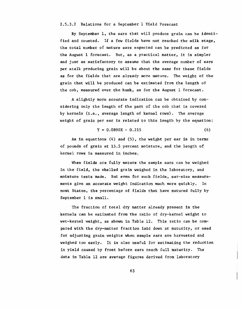
2.5.3.2 Relations for a September 1 Yield Forecast

By September 1, the ears that will produce grain can be identi-fied and counted. If a few fields have not reached the milk stage,ilietotal number of mature ears expected can be predicted as forthe August 1 forecast. But, as a practical matter, it is simpler~d just as satisfactory to assume that the average number of earsper stalk producing grain will be about the s~e fur these fieldsas for the fields that are already more mature. The weight of thegrain that will be produced can be estimated from the length ofthe cob, measured over the husk, as for the August 1 forecast.

A slightly more accurate indication can be obtained by con-sidering only the length of the part of the cob that is coveredby kernels (i.e., average length of kernel rows). The averageweight of grain per ear is related to this length by the equation:

Y = 0.0890X - 0.215 (6)

As in equations (4) and (5), the weight per ear is in termsof pounds of grain at 15.5 percent moisture, and the length ofkernel rows is measured in inches.

When fields are fully mature the sample ears can be weighedin the field, the shelled grain weighed in the laboratory, andmoisture tests made. But even for such fields, ear-size measure-ments give an accurate weight indication much more quickly. Inmost States, the percentage of fields that have matured fully bySeptember 1 is small.

The fraction of total dry matter already present in thekernels can be estimated from the ratio of dry-kernel weight towet-kernel weight, as shown in Table 12. This ratio can be com-pared with the dry-matter fraction laid down at maturity, or usedfor adjusting grain weights when sample ears are harvested andweighed too early. It is also useful for estimating the reductionin yield caused by frost before ears reach full maturity. Thedata in Table 12 are average figures derived from laboratory

63

studies for the North Central States during the early 1960's.Table 12 gives the relation between averages for large numbersof ears. Although anyone ear for which the ratio of dry-kernelweight to wet-kernel weight is 70 percent will have already laiddown all of its dry matter, a group of ears for which the averageratio is 70 percent must obviously include some ears for whichthe ratio is less than 70 percent. For this reason, the data inTable 12 indicate a slightly different relation than would havebeen observed for individual ears. Tables 13 and 14 are basedon individual ear data.

Table l2--Relation Between Ratio of Dry-Kernel Weight to Wet-Kernel Weight and Fraction of Total Dry Matter Laid Down

Average ratio Average Average ratio Averagefraction of fraction ofof dry-kernel total dry of dry-kernel total dryweight to wet- matter weight to wet- matterkernel weight laid down kernel weight laid down

(pet) (pet) (pet) (pet)

10 5 50 70

20 15 60 85

30 30 70 95

40 50 80 100

64

2.5.3.3 Characteristics Useful in Forecasting Kernel and EarWeight

Tables 13 and 14 show some correlation between various char-acteristics for corn. The tables suggest some of the possibleatlernative approaches which could be considered for corn on anyof the three dates, based on stage of development.

Table l3--Typical Kernel Characteristics and Correlation WithDry-Ear Weight by Days After Silking

Number Dry Wet Correlation betweenDays kernels dry-ear weight andafter per weight weight Number Dry- Wet-

silking ear per per of kernel kernelII kernel kernel kernels weight weight

(gm) (gm)

15 790 .048 .198 .45 ~I ~I

25 760 .120 .280 .45 ~I ~I

40 610 .225 .385 .90 .55 .4255 605 .255 .385 .80 .40 .3070 600 .260 .360 .84 .40 .30

85 600 .260 .355 .80 .25 .10

11 Based on a count of kernel with evidence of fluids orcoloring appropriate to stage of development.

~I Too few data points.

65

Table l4--Typical Correlation of Ear Characteristics With Dry-Ear Weight by Days After Silking

Maximum Kernel Total Cob SurfaceDays circum. surface length area Jjafter (after area !./ earsilking husk (husk weight over (over

removed) removed) (wet) husk husk)

15 .70 .75 .70 .60 .65

25 .50 .75 .75 .65 .75

40 .50 .85 .85 .75 .75

55 .65 .85 .90 .75 .85

70 .65 .90 .90 .82 .92

85 .65 .90 .90 .70 .85

!./ Average kernel-row length times maximum circumference.

l/ Cob length times maximum circumference.

2.5.3.4 Relations for an October 1 Yield Forecast

By October 1 all dry kernel weight has been laid down inmost fields. But, in a few fields, the weight of grain per earmust be estimated by ear-size measurements or other means.

The most accurate indication can be obtained by weighingsample ears and applying the relations in Table 12 to adjust theobserved grain weight to a weight at maturity. But if the pro-duction of dry matter is halted by a killing frost before theears have a chance to reach maturity, an allowance must be madefor the resulting reduction in yield. When the moisture contentis known, Table 12 can be used for this purpose.

66

2.5.4 Forecasts Based on Growth Models for Yield Components

Within-year growth models for forecasting components havebeen investigated. These methods rely on plant data only fromthe current year. As such, they have the opportunity of reflect-ing unique characteristi6s of the crop year for which the forecastis desired. However, the same type of growth model is assumedeach year and statistical estimates of the model parameters arederived for the current year.

Within-year models depend on relating a response (the com-ponent to be forecast) to values of a second variable which has aknown value at maturity. Various measures of time or a variablewhich reflects the aging of the component provide a suitableindependent variable for this purpose. In fact, Table 12 is anexample of a relative growth model based on percent of dry matteras a time or aging variable.

In modeling the average weight of grain per ear per plant forcorn, "days since silking" has been considered as the time variable.Note the uniformity of weight after physiological maturity inTable 13. The model provides an estimate of grain weight at anygiven time after silk emergence. The forecast is dependent on howwell the model represents the actual situation and on our abilityto know what value of time corresponds to maturity and how to mea-sure these accurately. In this case, the time value at maturityis any value in the plateau region.

Within-year models for survival (the complement of the growthmodel) of the fruit, ears, or other characteristics may also bedeveloped. The forecast of the number of ears is then combinedwith the growth model for weight per ear. The dependence of asurvival ratio on days since a base date for plants with ears peracre is used to forecast number of ears at maturity. The base dateof plants with ears per acre is defined to be day zero for the sur-vival ratio. The forecasted survival ratio at maturity is multipliedby the base estimate of plants per acre with ears to adjust it to

67

number of units at harvest. Under conditions in the U.S., thisratio is about .98 to .95 for corn ears and has no known relationto the yield estimates.

Research on both growth and survival models has also beenfound applicable to several crops. For example, survival modelshave been investigated to forecast the portion of papayas set eachweek surviving to harvest (some five to six months later), as wellas used as a growth model to forecast weight per grape. Becauseprevious year data are required for developing over-the-year models,within-year methods may be more applicable in developing and imple-menting objective yield forecast procedures for new crops. However,it is assumed that the basic models are known from other studiesor research.

The general form of the logistic growth model which is commonlyutilized is:

yt

An alternative but equivalent form is:

yt

This is a nonlinear model, where t is the independent time variable,Y is the dependent variable, and a, e and p are the parameterst

which can be estimated from data sets of the form:

68

In the application discussed here, Y is the estimated mean dryt

weight of corn per ear or per kernel at time t. The variable tis the time (days) after one of the phenological events: tasselemerged, silks emerged, silks starting to dry, silks finisheddrying; or the "time" variable can be dry matter fraction of thegrain when sampled.

The basic model uses repeated observations from the currentyear to estimate the parameters needed to predict the dependentvariable (dry weight of grain per ear, per plant or per kernel)at maturity. The model parameters may be updated at various timesduring the growing season as more data become available for laterstages of growth. The same type of model is used each year, butthe parameters derived from the data would relate to: (1) thecurrent year, and (2) a given cutoff time within the growth period.Since three parameters are to be estimated, at least three observa-tions within a season are required.

The role of the three parameters in the growth model can bedescribed in terms of various phases of growth.

1. The initial phase or base weight is at t = O. Since p(whatever its value) raised to the power t = 0, is 1,

Y =o1

a + Sestimates the base weight or initial weight.

2. The final phase or mature forecast weight of the depen-dent variable is the most important in forecasting finalcorn yield. Assuming that O<p<l, we see that the fore-

cast harvest weight is Ym

lim Yt-+oo t

1=-;::-. That is, for

the point estimate, a", is the fore-

large values of t, Y depends upon a Therefore, thet

parameter a is termed the primary parameter. For thealternative form of the logistic growth model,

a1 + B .. ~ .. t

cast of dry-kernel weight per plant at maturity.

69

3. The intermediate phases of growth follow the initial phaseand continue until maturity, when the large values of tare reached. The value of p reflects the rapidity of theweight increase from YO to Ym as t increases. For O<p<lthe model is indeed a growth model and p can be termed therate-of-growth parameter. If p is near zero the growth isvery rapid. If p is near unity, growth at a gradual rateis indicated. The ratio of

Y(3m 1 +-= AA

Yo exdetermines the range of the Y scale.

t

set were ex = .006, (3 = .08, and p = .87.

The computer programs utilized to derive the parameters fromthe data require approximate starting values, since fitting non-linear equations is based on iterative algorithms. For the dependentvariable dry weight per ear, the starting values used for the data

For Y = dry weight pert

kernel at time t~,the initial or starting values used were ex = 3.8,(3 = 130, and p .87. Normally, the values from a previous yearcould be used to start the iterative algorithm.

Each set of parameter estimates defines a specific model ata given time. For example, for 1973 in Central Iowa, Y = dry

tweight (gm) per ear at t days after silks begin to dry, and wehave the following parameter estimates for data sets availableafter various field visits given in Table 15.

70

Table l5--Estimates of Model Parameters Based Upon All DataAvailable After Various Field Visits

No. of visits (during season)Parameter Four Six Seven Eight Nine

(IV) (VI) (VII) (VIII) (IX)

0. .0059597 .0061557 .0062934 .0063149 .0063487

13 .12777 .12930 .14616 .14869 .15380

p .88271 .88108 .87514 .87428 .87267

Thust the specific model based upon data obtained on fieldvisits I-VII is

Y :0:t

1

.0062934 + .146l6(.875l4)t

where Yt is the estimated dry weight (gm) of grain per ear att days after silks began to dry. For Y ~ :0: estimated dry weight

t(gm) per kernel at t~ days after silks emerged, based upon datafrom visits I-VII, the model is

y ~t

1

3.8654 + 333.95(.87113)t~

Numerical values of the dependent variables for variousvalues of the two time variables are shown in Table 16 for thesetwo models.

71

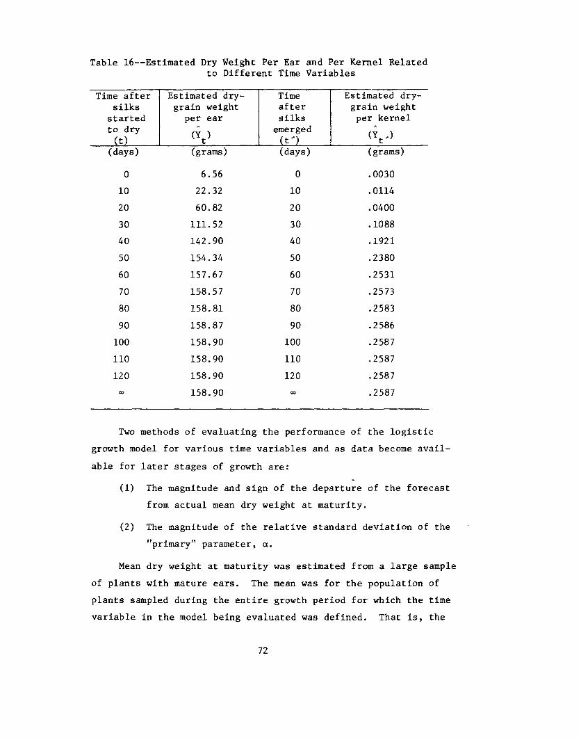
Table l6--Estimated Dry Weight Per Ear and Per Kernel Relatedto Different Time Variables

Time after Estimated dry- Time Estimated dry-silks grain weight after grain weight

started per ear silks per kernelto dry ~ emerged ~

(Y ) (Y ,)(t) t (t') t(days) (grams) (days) (grams)

0 6.56 0 .003010 22.32 10 .011420 60.82 20 .040030 111.52 30 .108840 142.90 40 .192150 154.34 50 .238060 157.67 60 .253170 158.57 70 .257380 158.81 80 .258390 158.87 90 .2586

100 158.90 100 .2587no 158.90 110 .2587120 158.90 120 .2587

co 158.90 co .2587

Two methods of evaluating the performance of the logisticgrowth model for various time variables and as data become avail-able for later stages of growth are:

(1) The magnitude and sign of the departure of the forecastfrom actual mean dry weight at maturity.

(2) The magnitude of the relative standard deviation of the"primary" parameter, a.

Mean dry weight at maturity was estimated from a large sampleof plants with mature ears. The mean was for the population ofplants sampled during the entire growth period for which the timevariable in the model being evaluated was defined. That is, the

72

model forecast and estimated mean weight make valid inferences aboutthe same subpopulation. The relative standard deviation is the esti-mated standard deviation divided by the estimate of the primary

(1( _a.)parameter n

For the two examples previously discussed, departures of theforecast from the actual mean dry weight and ,the relative standarddeviations are shown below.

Table l7--Percentage Difference Between Forecast and Harvest Weightand Between Relative Error in Primary Model Parameters

RelativeInde- Departure of standard

Dependent pendent Data from forecast from deviation ofvariable time visits actual mean estimate of

variable dry weight primaryparameter (a)

(pet) (pet)

Dry Days I(only) (No convergence to mode1)weight after I & II +22.0 34.46of silk I - III +0.7 6.96grain starting I - IV +7.8 4.32per to dry I - V +8.5 2.74ear (t) I - VI +4.4 1.74(Y ) I - VII +2.1 1.29t I VIII +1. 7 1.16-

I - IX +2.2 1.02I - X +1.2 0.92

--------------------------------------------------------------------

Dry Days I(only) -89.6 16.07weight after I & II -71.4 12.09of silk I - III -37.3 10.10grain emerged I - IV +4.6 6.61per (t") I - V -6.0 2.24kernel I - VI -1.8 1.59(Y .•) I - VII +0.4 1.37t I VIII +0.5 1.15-

I - IX +0.9 0.98I - X +1.2 0.86

73

2.5.5 Forecasting Methodology for Citrus Yields

2.5.5.1 Introduction

The program for estimating the citrus crop in Florida wasdeveloped in the late 1950's. The yield estimating portion ofthe program as it was originally developed and put into opera-tion is discussed in this section. Most of the methodology anddata concepts have remained unchanged.

The inventory of trees by type, age, and location is veryimportant in the forecasting of current yield and productionbecause of the dynamics of the industry. It is needed to pro-vide a complete and efficient sampling frame of trees for samplesurveys designed to estimate the number of fruit per tree. Theinitial yield survey each year is used to estimate the averagenumber of fruit per tree. This survey begins August 1 and con-tinues to September 15. It is referred to as the "limb countsurvey."

2.5.5.2 Estimating Average Number of Fruit Per Tree

Number of fruit per tree varies considerably due to differ-ent ages and locations. Most citrus trees start bearing about3 to 4 years after planting. Production increases rapidly forabout 10 years, tapers off, and reaches maximum about 25 to 30years after planting. These tree characteristics and the vitalknowledge of tree numbers by age and area allow considerablereduction in estimator variances by using a stratified sampledesign. Prior knowledge of fruit counts by age of tree was usedto construct strata.

Stratum

1234

74

Age of Tree(years)

4- 910-1415-2425 and older

The relatively small counts on trees in stratum 1 and thesmaller variances of these counts combined with the large influxof young trees into the universe allow increased efficiency byusing optimum allocation of sample to age strata.

Since the age-type blocks are too large to be feasible unitsfor counting fruit, the groves are subsampled to obtain a clusterof trees. From variances on complete tree mappings (i.e., censuseson individual trees), it was determined that a limb of area equiva-lent to 10 to 20 percent of the main trunk area could be countedand the count expanded to obtain a fairly efficient estimate offruit population for the total tree. The sample sizes of numberof groves and number of trees per grove were determined from ex-panded counts made on randomly selected limbs which constitutedapproximately 10 percent of the main trunk area as determined bymeasuring the circumference with a tape. Data were summarizedusing analysis-of-variance techniques for a hierarchical classi-fication. Computed variances were used for optimum allocation ofsample to age strata.

B. W. Kelly conducted the pilot survey work on 50 trees in1956, providing estimates of variance components, required samplesize, and optimum allocation. The results are presented in Table 18.Subsequent analyses of variance on estimated fruit per tree from thelimb count surveys indicated the pilot survey to be relativelyaccurate.

An aerial tree census is the source of the list of all blocksof each major type of citrus in the State from which the blocksare selected. A block of citrus is not defined by ownership butrather is defined as being a relatively homogeneous planting withat least 90 percent of the trees being of the same age and citrustype. The block identification, tree numbers, and accumulatedtree numbers are listed by county and by date of planting for eachtype of fruit (a type consists of one or more similar varieties).A sample of blocks is selected for each type of citrus.

75

Table l8--Estimated Limb-Count Variance Components, 1956

Components of variance 1/ Indicated'VIndicated

Type of (nested design) optimumfruit sample trees

County Age Grove Tree size pergrove

OrangesMidseason 0 43 118 360 519 3.5Late 7 84 162 93 463 1.5

All 499

GrapefruitSeedy 12 0 20 218 294 6.5Seedless 20 3 69 152 418 3.0

All 370

11 Variance components for number of fruit per tree estimated bylimb count method. Variance components rounded to nearestthousand.

II Indicated number of groves required for a maximum of 4 percentsampling error (coefficient of variation at .95 level of con-fidence), assuming 4 sample trees per sample grove.

After the sample groves are selected, a "pivot tree" ischosen in each sample grove. The pivot tree in each case specifiestwo sample clusters of four trees each; clusters are rotated tominimize the effects of working in the trees to make fruit counts.The procedure used to designate pivot trees allows the proper pro-portions of outside trees to be selected. Due to demise, or toimproper age or type, it is sometimes necessary to substitute fora sample tree using a predetermined substitution pattern.

The third and final stage of sampling pertains to selection ofa portion of the tree on which the fruit is to be counted. Countsare made on sample limbs selected by the random-path technique.When this multiple-stage process terminates, the selected limb(branch or group of branches) has a probability of selection pro-portional to limb cross-sectional area (c.s.a.). The reciprocalof this probability of selection affords an unbiased method of

76

expanding sample counts to estimated total fruit on the tree and,due to the positive correlation between c.s.a. measurements oflimb size and number of fruit, is a fairly efficient method ofsampling. Proof of the unbiasedness of the estimator, (x./P.),

1 1

and derivation of the probability, (Pi)' are given elsewhere.

Application of the random path selection method is fairlysimple. Branches of the primary tree scaffold (first majorbranching) are measured with a tape which shows c.s.a. in squareinches. The c.s.a. and cumulative c.s.a. square inches are re-corded for each limb on the field sheet where "limb" is definedas being a branch or grouping of adjacent branches totaling 10percent or more of the cumulative total c.s.a. at the firstscaffold level. A number selected from a random-number tabledetermines the individual portion selected. A logical alternativeto the 10-percent sample limb would be two 5-percent limbs. How-ever, smaller limbs appear to have a lower correlation betweenc.s.a. and fruit count.

The principle involved in the "limb count" selection isdepicted in Figure 2 on page 84. The procedure by stages includesmeasurement of the first scaffold c.s.a. to determine that approxi-mately a 19-inch limb (10 percent of 190 square inches) is neededto provide the sample unit. The route toward the sample limb isdetermined by a random number from 1 to 190 and the accumulatedc.s.a. measurements. In the example, the 100-inch limb wasselected by the random number. This limb had a probability ofselection of 100/(100 + 90). At the second scaffold the illus-trated selection was the 20-inch limb, and the 187 fruit on thatlimb were counted. The probability of selection at the secondstage was the first-stage probability times the second-stageprobability, given that the first-stage selection is known. Inthe example, then, the probability of the 20-inch limb's beingthe sample limb is:

100 20 100 20 20100 + 90 x 20 + 40 + 50 = 190 x 110 = 209

77

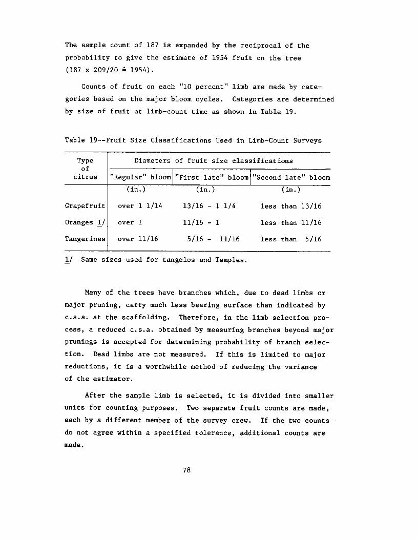
The sample count of 187 is expanded by the reciprocal of theprobability to give the estimate of 1954 fruit on the tree(187 x 209/20 = 1954).

Counts of fruit on each "10 percent" limb are made by cate-gories based on the major bloom cycles. Categories are determinedby size of fruit at limb-count time as shown in Table 19.

Table 19--Fruit Size Classifications Used in Limb-Count Surveys

Typeof

citrus

Diameters of fruit size elassifications

"Regular" blooml"First late" blooml"second late" bloom(in.) (in.) (in.)

Grapefruit

Oranges 1..1

Tangerines

over 1 1/14

over 1

over 11/16

13/16 - 1 1/4

11/16 - 1

5/16 - 11/16

less than 13/16

less than 11/16

less than 5/16

1/ Same sizes used for tangelos and Temples.

Many of the trees have branches which, due to dead limbs ormajor pruning, carry much less bearing surface than indicated byc.s.a. at the scaffolding. Therefore, in the limb selection pro-cess, a reduced c.s.a. obtained by measuring branches beyond majorprunings is accepted for determining probability of branch selec-tion. Dead limbs are not measured. If this is limited to majorreductions, it is a worthwhile method of reducing the varianceof the estimator.

After the sample limb is selected, it is divided into smallerunits for counting purposes. Two separate fruit counts are made,each by a different member of the survey crew. If the two countsdo not agree within a specified tolerance, additional counts aremade.

78

A random selection of one of the 10-percent limbs in a 10-percent random subsample of limb-count groves is made as a qualitycheck of the original counts. These quality checks indicate thatthe method provides a fairly consistent undercount of about 1 per-cent.

2.5.5.3 Forecasting Fruit Drop

A measure of fruit mortality prior to harvest must be intro-duced into computed crop forecasts, because initial estimates ofthe average number of fruit per tree are established from countsin August and September. Natural loss of fruit, from August untilthe month in which each type of fruit is considered mature, ismeasured by a sequence of monthly surveys. Maturity is consideredto be reached in predetermined cutoff months which precede theheaviest harvest period. Cutoff months are: December for tangelosand tangerines, January for early and midseason oranges, Februaryfor Temples and grapefruit, and April for late-season oranges.

The sample trees for droppage surveys are drawn from a specialor a restricted portion (blocks along roads) of the frame used forthe limb count. Blocks along this route frame are readily accessiblefor monthly observations. This sample frame consists of all bearingcommercial groves fronting on a 1,500-mile route which traversesproducing areas of the most important counties. This microcosm ofthe citrus population provides a satisfactory base for samplingdrop and other relatively uniform characteristics.

The sample for each variety is stratified into four areas(homogeneous county groupings) and the four age groups previouslydiscussed. The sample size within strata is based on productivityin a base year.

A sample limb approximately two percent of the trunk c.s.a.is selected near shoulder height, on a designated side of the tree.This limb is tagged and all fruit beyond the tag are counted during

79

successive surveys. The differences between the initial surveycounts and later survey counts indicate the droppage to the timeof the survey. The average drop for each age-area is computed andthen combined by production weights into the average drop for theState. The sample counts are weighted, because groves are selectedwith probability proportionate to production and the "two percent"limb sample survey tends to put a disproportionate part of thesample in older, more productive trees.

The monthly drop rates are adjusted by the estimated propor-tion of total crop harvested by the survey date. The accumulatedfruit drop represents only those groves not yet harvested. Theadjusted monthly droppage is projected to the cutoff month to esti-mate seasonal drop rate for use in the forecast models.

The 2,000-tree sample in 1966-67 indicated the proportion oforanges remaining for harvest with a maximum error of three per-cent at the .95 level of confidence. The sampling errors of thedrop survey are expressed as the coefficient of variation for theproportion of fruit remaining to be harvested, since this is theerror contribution to the production forecast.

Prior to the 1970-71 season, monthly projections of fruit lossexpected to occur prior to the cutoff month were made by graphicinterpretation of charts similar to those in Figure 3 on page 85.Although this procedure was satisfactory during years in whichloss of fruit was within the normal range, experiences in recentseasons suggested that visual interpretation was not sufficient,particularly when the rate of drop was much higher or lower thanusual. Starting in 1970, multiple-regression formulas have pro-vided additional means of estimating total fruit loss.

80

2.5.5.4 Forecasting Average Harvest Size of Fruit

The fruit-size survey coincides with the drop survey. More-over, the same subsample of trees in sample groves drawn from theroute frame is used for both sets of monthly observations. In thesize survey, 10 sample fruit per tree are measured from a two-treecluster per sample grove. Frequency distributions of standardfresh-fruit sizes and the estimated average size are obtained eachmonth.

The fruit to be measured are determined by a "random grab"or point on the tree about shoulder height. This point on thetree is tagged and, for each survey, horizontal circumferencesare measured on the 10 regular bloom fruit nearest the tag.

These circumference measurements are entered as a tally onthe 240-cell field form. Summarization is done in volume, whichis linearly correlated with weight and, therefore, is additive.The weight-to-volume relation has a correlation coefficient squared(r2) 0f 96 hi hi· d···. , w c s pert1nent to a pro uct10n est1mate, S1ncemost of the citrus crop is received or purchased on a weight basis.

Figure 4 on page 86 depicts the growth rates of two citrustypes. The dates shown are the months in which surveys were con-ducted; usually surveys were near the third week of each month.The annual growth curves generally parallel each other, therebyallowing these relationships to be a fairly effective tool inforecasting size at maturity. It should be noted that fruit mea-sured on-tree does not reflect harvest size. (Early observationsare of immature fruit, and measurements for forecasts usually ceaseprior to the main or volume harvest.) The size of fruit at maturityis defined as the average size of fruit in groves in a specificmonth. These cutoff months are the same as in the drop surveys.Prior to the cutoff month, it is necessary to estimate the averagesize that fruit will attain in the cutoff month.

81

A regression using three variables is used to forecast size(volume per fruit) at the cutoff month:

X 4.34 + .964Xl - .159X2 - .002X3 (for early-mid oranges

on the October 1 forecast date)

and r = .95, where the three variables are (1) current month'saverage size in cubic inches, (2) growth during the preceding month,and (3) average number of fruit per tree for that type. The multi-ple regression has provided a sounder indication of final size thana subjective evaluation of the importance of these factors inarriving at a forecast size. In 1967-68 a subsample of fruit on1,200 sample trees used in size surveys provided a maximum errorat the .95 level of confidence of about 1.5 percent in averagefruit size for all oranges.

The citrus check data, with which the forecast must be com-pared, is the number of certified boxes harvested--90-pound boxesfor oranges, tangelos and Temples; 95-pound boxes for tangerines;and 85-pound boxes for grapefruit. The forecasted average volumeper fruit is converted to number of fruit constituting a box bygraphic means, as shown in Figure 5 for grapefruit. This numberdepends upon type of fruit, size of fruit and whether the fruitis sold for the fresh market or is used in processing. Curvilinearrelationships were also fitted by equations of the form

S = a + bX + i 'where S is the average number of fruit per boxand X is the average size of fruit. For early-mid oranges theequation is:

S = 53.77 - 1.696X+ 22i9.5

Coefficients for the fresh and processed lines are then weightedtogether by utilization of the crop (previous season's proportion)to provide a basis for converting average volume of each type to"fruit per box." This method of converting volume to fruit perbox also compensates for the deviation from spherical shape inconverting circumference to volume.

82

2.5.5.5 Forecasting Yield Per Tree

Two models have been used to combine the components whichdetermine citrus yields: A direct expansion estimator and therelative change estimator. Only the direct expansion estimatoris given; that is,

Y = F x HS

whereY = yield per tree in boxes of fruit

F = number fruit per tree at time of limb-count survey

H = proportion of fruit to be harvested

S = harvest size of fruit expressed in fruit per box

The relative importance of the factors contributing to changesin production is shown in Figure 6 on page 88.

83

Figure 2: Random Limb Selection With Probability Proportional to Cross-Sectional Area

100P ••1 100+ 90

(187

~ ( Fruit

\. ,20"

""-- "'-P2 20

20 + 40 + 50-

Estimated Fruit per Tree

F i Co 1 1 187 100+ 90 20 + 40 + 50 •ru t unt x - x - •• x ---- x ------- ••P1 P2 100 20 1954

84

Figure 3:

PercentDrop

Fruit Drop CurvesExtreme Years and Average of 1963 - 1969 Seasons

Early - Midseason OranRes1969-70

1816141210

8

6

4

2

o

PercentDrop

Sept. Oct.

Valencia Oranges

85

Nov. Dec.

1969-70

Average

1968-69

Figure 4: Fruit Growth CurvesExtreme Years and Average of 1963-1969 Seasons

Size(cu. in.)

EarlY-Midseason Oran~e8

13

9

8

7

6

~-----------------------------------

1966-67- - - Average....•...•..• - ...

1965-66

Dec.Nov.Oct.

10

Size(cu. in.)

Valencia Oran~e.

-- - ---- - - - Average---- - - - 1969-70,-~,,..,

",,,,....,....,.'

1963-64

I

Mar.I

Feb.I

Jan.I

Dec.,

Nov.

,Oct.Sept,

I

Aug.

6

5'l

86

Figure 5: Converting Volume to Fruit per ~ox. Seedless Grapefruit

Fruitper Box

120

110

100

90

80

70

60y

p•.Y - .46 Yp + .54 I,

L ,....L.------''------ -----------y-,25 30 35 40 4S

Size of Average Fruit (Cubic Inches)

87

Figure 6: Relative Importance of Factors Affecting AverageAnnual Change in Florida Citrus Production

1960-61 to 1967-68

Early and Midseason Oranges Valencia Oranges

Seedless Grapefruit

88

2.6 Simulation Models Based on Plant Physiology

2.6.1 IntroductionCrop-growth simulation models which consider the soil-plant-

atmosphere continuum have only recently been introduced. Theimpetus to develop crop-growth models involving the plant environ-ment resulted from the successful modeling of photosynthesis. Todate such models have been developed for corn, sorghum, cotton,alfalfa, barley, and wheat. The utility of these models has beenas crop management and research tools. However, the modificationof these deterministic models to forecasting crop yields for largeareas requires knowing the plant environment for each day of theentire growing season, as well as detailed knowledge of the plantand how it functions in this environment. These relations arebased on how the major plant parts respond each day to theirenvironment.

A brief account is presented of an approach due to Arkin,Vanderlip, and Ritchie for calculating the daily growth and develop-ment of an average sorghum plant in a field stand. The appearanceof leaves, their growth rate, and the timing of these events aregrowth characteristics incorporated in the model. It should beclear that the objective is to model the entire plant cycle andnot just the reproductive phase of the plant's life. Consequently,the adaptation of these models to forecasting yield requires veryexact modeling of the yield components and realistic simulation ofthe daily climatic inputs for the entire growing season.

2.6.2 The Model

The physical and physiological processes of light interception,photosynthesis, respiration, and water use are independently modeledand used as submodels. The accumulated dry weight (or yield) forthe crop is the product of the plant population and the modeledweight for the "average" plant. Most of the equations describingthese processes are empirically derived from field and controlled

89

Figure 7: Flow Chart for Sorghum Simulation Model

PlantFeedback

Calculate DailyLight

Interce tion

Calculate DailyPotential

Photos nthesis

Calculate DailyDry-Matter Gainof Plant Parts

90

Table 20--Input Data Required for Sorghum Simulation Model

A. For Model Without Feedback Data

Plant DataLeaf number: total number of leaves produced 2Leaf area: maximum area of each individual leaf, cm

Planting DataPlanting date: month, day, yearPlant population: p1ants/haRow width in cmRow direction in degrees

Climatic Data (daily from planting to maturity)Maximum temperature, °c

°Minimum temperature, CSolar radiation, 1y/dayRainfall, cm/day

Soil DataAvailable water-holding capacity, cmInitial available water content, cm

Location DataLatitude in degrees

B. For Model With Plant Feedback Data - for Specific Date(s)During Growing Season

Number of leaves fully expandedNumber of leaves emerged but not fully expandedLeaf weightCulm weightHead weightGrain weightRoot weigh tSoil waterLeaf area indexLeaf area of individual leaves

91

experiment measurements. The model operates on a daily basis, and,therefore, only daily climatic inputs are required. Other inputsare initialized (i.e., assumed) at the outset of the modeling run.A generalized flow diagram of the model is given in Figure 7. Theinputs required are shown in Table 20.

2.6.2.1 Seedling Emergence

Seeds imbibe water at very low soil-water contents. There-fore, seedling emergence as calculated is assumed to be dependenton temperature only. Mean air temperature is used in the com-putations of days until emergence. It was determined thatapproximately loDe is the threshold soil temperature belowwhich seedling emergence will not occur. The relationshipbetween heat units above the threshold derived from averagetemperature (i.e., (max + min)/2) and day of emergence islinear.

2.6.2.2 Leaf Number and Area Development

To determine the amount of light (photosynthetically activeradiation (PAR) in the .4 to .7 ~ wave band) intercepted by thegrain sorghum plant canopy, the leaf area per plant must be known,since the amount of intercepted light is primarily dependent onleaf area. In turn, plant dry-matter accumulation (weight gain),mainly a consequence of photosynthesis, is light dependent. Leafarea per plant is also needed for calculating transpiration whenthe plant canopy provides only a partial ground cover.

Leaf area development was modeled from inputs of number ofleaves produced by the hybrid planted and the maximum area of aleaf. Both field and phytotron studies have shown that the rateat which leaves appear out of the whorl on the grain sorghumplant and the rate at which leaves expand out of the whorl arerelated to mean daily temperature (or heat units) when plantsare adequately watered.

92

Leaf appearance rate is calculated by summing daily heatounits above a base temperature of 7 C. A new leaf is initiated

each time 50 heat units are accumulated. Leaf extension rateis computed in a somewhat similar fashion. Daily leaf area iscalculated by summing the new leaf area each day for the expand-ing leaves and the leaf area of the plant computed the day before.Leaf senescence (death or "firing") results in a reduction of leafarea.

2.6.2.3 Canopy Light Interception

Leaves on the plant overlap one another and neighboringplants may shade one another. Thus, not all of the plant's leafarea is actually intercepting light. Shading in the plant canopyis dynamic and changes with the sun's altitude and azimuth andwith plant size. To account for these interactions, a mathematicalmodel for computing ligh~ interception in a grain sorghum plantcanopy was developed. The light interception by a plant in thecanopy is computed using a modification of the Bouguer-Lambertequation (commonly referred to as Beer's Law).

2.6.2.4 Potential Net Photosynthesis

Potential net photosynthesis, defined as the net CO2 fixedduring the daylight hours on a ground area basis for nonlimitingwater and temperature cor.ditions,was calculated using relationsdeveloped from data obtained from a canopy gas-exchange chamberand simultaneous light interception measurements.

2.6.2.5 Daily Net Photosynthesis

A series of efficiency functions which reflect the effectsof nonoptimum ambient temperature and soil-water conditions onplant growth are used in the model. Each efficiency parameteris a dimensionless fraction with a value from 0 to 1. A multi-plicative relation is developed for computing net photosynthesis.This expression for net photosynthesis was based on the hypothesi~

93