1

San Diego Bay Terrain Model

FINAL REPORT

Richard M. Gersberg, Ph.D, Principal Investigator San Diego State University Research Foundation

A Project Supported by the San Diego Unified Port District

January, 2014

2

ABSTRACT A seamless bathymetric/topographic Digital Terrain Model was developed for the first time for San Diego Bay. This model combined the new (2012) LiDAR DEM that was available from LiDAR data for 2009-2011 by NOAA’s Digital Coast, Coastal LiDAR Project and the latest high resolution bathymetry data generated by Dr. Neal Driscoll at the Scripps Institute of Oceanography (SIO). We then used this Digital Terrain Model to better quantify the impact of sea level rise on coastal wetland habitats. Using the SLAMM (Sea Level Affects Marshes) Model, we delineated the effect of sea level rise on San Diego Bay’s ’s wetlands including the jurisdictional wetlands of the San Diego Unified Port District. Additionally, we used SLAMM to predict future alterations of the San Diego Bay National Wildlife Refuge including the Sweetwater Marsh Unit and the South Bay Unit. This modeling allows the prediction of wetland inundation (and associated habitat change) under the range of plausible sea level rise scenarios. This in turn allows a better understanding of how these habitats will be altered in the future, and how these changes will impact the plants, birds, and fish they support, and supports adaptive management and planning strategies. We also used the seamless Digital Terrain Model developed specifically for San Diego Bay to define the potential impacts of sea level rise on the eelgrass habitats of San Diego Bay, and specifically, and to delineate the specific effects of sea-level rise on submerged eelgrass beds in San Diego Bay.

3

INTRODUCTION

Estuaries, with their shallow water (saltmarsh and eelgrass) habitats, are at the boundaries of land and ocean. Because of their unique position in the landscape, they provide many important ecological services that maintain and improve the health of our environment. These shallow water estuarine ecosystems provide nursery grounds and foraging habitat for hundreds of species of fish, shellfish, birds, and mammals. However, occupying the coastal fringe as they do, these habitats will also be among the first to suffer the impacts of sea level rise. Under a rising sea level associated with global climate change, some aquatic habitat types are likely to gain in extent as the intertidal zone becomes submerged, while certain intertidal marshes and submerged types of aquatic vegetation (e.g. eelgrass) will be lost. Such loss of these habitat types is of real concern in the San Diego region in part due to relatively small acreage remaining, their vulnerability to development activity, and their relatively high value as habitat. Furthermore, the larger the changes and rate of change, the harder it will be for most fish and wildlife species to adapt to the impacts of global warming.

Sea level rise may be attributed to two main factors: the thermal expansion of ocean waters due to increased global temperature, and the increased discharge of water from melting glaciers and the Greenland and Antarctic ice sheets. If a natural coastal marsh cannot build itself vertically (through accretion) to keep up with the rising sea level, then eventually it will be totally inundated and be converted to tidal mudflats or open water. Accretion rates vary spatially among wetlands, and are dependent on both autochthonous productivity within the wetlands itself, but also, upon sediment delivery from upland processes and transport. Sea level rise impacts on a coastal wetlands also depend on the wetland’s potential for inland migration. Given the appropriate slope/elevation and land use condition, wetlands can migrate landward as a response to sea level rise. That is, if a wetland can keep pace vertically with sea level rise and there are no barriers to inland migration (such as sea walls, naturally occurring cliffs, or roadways), then over time the landward wetland boundary will migrate inland as uplands are converted to wetlands. So depending upon the elevational landform of the coast as well as the land use patterns of the near-coastal upland areas, the total wetlands area may increase, decrease, or remain the same as the marsh migrates inland.

Additionally, in San Diego Bay, eelgrass beds are considered to be a valuable shallow-water habitat, providing numerous ecological services including: shelter, nutrient cycling, or breeding habitat for many species of invertebrates, fishes, and some waterfowl. Eelgrass beds also stabilize sediments and provide organic material to nearshore environments. These plants grow in relatively few locations within the Bay and require special conditions to flourish.

Sea-level rise will have a variety of effects on eelgrass habitat. Increased water depth will restrict the amount of light reaching eelgrasses, and depending on the bathymetry of the Bay and topography of the surrounding landscape, change the geographic distribution of the eelgrass habitat. Based upon our current understanding of eelgrass distribution, it does indeed seem likely that sea level rise will move the maximum depth of eelgrass growth and abundance closer to the current shoreline.

Key concerns include sea level rise, coastal wetland alteration, possible eelgrass habitat loss, and San Diego’s adaptation to sea level rise. The IPCC’s (Intergovernmental Panel on Climate Change) latest Assessment Report 5 (IPCC, 2013), estimates that the likely range of sea level rise in 2100 for the highest climate change scenario is 52 to 98 centimeters (20 to 38 inches). In the same report, the risk of exceeding 98 cm is considered to be 17%, which brings the upper end closer to about 1.2 m. Furthermore, the IPCC adds in the caveat that “several tenths of a meter of sea level rise during the 21st century” could be added to this if a collapse of marine-based sectors of the Antarctic ice sheet is initiated. Thus, looking at the upper value of the likely range, we end up with an estimate for the upper limit by 2100 as closer 1.5 meters

4

However, at the same time, a number of semi-empirical model projections of sea level rise have recently been developed. Many of these studies suggest that the upper end of the range of sea level rise projections by 2100 could be significantly higher than the IPCC projections (Nicholls et al., 2011). For example, using a correlation between observations of past changes in sea level with post-industrial era temperature changes, Rahmstorf (2007) projected a 0.5-1.4 m rise of sea level by 2100. Vermeer and Rahmstrorf (2009) refined this method with a rapid-response term which yielded an upper value of 1.9 m by 2100. Rohling et al. (2008) conducted a paleo-climate reconstruction and concluded that 2.4 m was an upper constraint to sea level rise by the end of the twenty-first century, and Lowe et al. (2009) using the research of Rohling et al. (2008) adopted a maximum global sea level rise of 2.5 m by 2100. Moreover, Pfeffer et al. (2008) considering kinematic constraints on glacial conditions, concluded that a sea level rise of 2m by 2100 could occur under physically possible glaciological conditions, and that the 2m value could well be considered the plausible upper end of the range for sea level rise by 2100.

SPECIFIC OBJECTIVES

Specific objectives of the San Diego Bay Terrain Model project include:

1. Develop a seamless San Diego Bay Digital Elevation Model in order to better quantify the impact of sea level rise on coastal wetland habitats.

In order to predict changes to coastal habitats in response to sea level rise, an accurate, and high-resolution terrain model is needed for San Diego Bay. In order to do this we coupled a new high-resolution LiDAR digital elevation model of San Diego Bay (recently made available by NOAA through Digital Coast), with the high resolution bathymetry developed by Dr. Neal Driscoll at SIO, to generate a relatively seamless digital map of San Diego Bay’s terrain

2. Using the SLAMM (Sea Level Affects Marshes) Model, delineate the effect of sea level rise on San Diego Bay’s ’s wetlands including the jurisdictional wetlands of the San Diego Unified Port District, as well as the wetlands of the National Wildlife Refuge including the Sweetwater Marsh Unit and the South Bay Unit. This modeling will allow prediction of wetland inundation (and associated habitat change) under the range of plausible sea level rise scenarios. This will allow a better understanding of how these habitats will be altered in the future, and in turn, how these changes will impact the plants, birds, and fish they support.

3. Using our coupled seamless Digital Elevation Model of San Diego Bay, define the potential impacts of sea level rise on the eelgrass habitats of San Diego Bay, and specifically, to delineate the specific effects of sea level rise on submerged eelgrass beds in San Diego Bay.

5

METHODS Development of Seamless San Diego Bay Digital Elevation Model The original Seamless San Diego Bay Elevation Model was created as a mosaic of both Bathymetry and Elevational Models. The new San Diego Bay DEM was created from three different sets of data. All of the datasets were converted to NAD 83 UTM Zone 11 (meters) as the horizontal coordinate system and their vertical datum was converted to NAVD 88 (feet). The datasets are identified as follows: times_mos_li1- this dataset was originally derived from the Corps Lidar data. It was mosaicked and then its horizontal coordinate system was converted from Geographic NAD83, GRS80 to NAD83 UTM (meters). Its vertical datum was in NAVD88 already. The vertical units were converted to feet. The cell size is 1 meter but was converted to 10 meters during the mosaic process. Minus_bathy_1- this dataset was originally derived from SDBay_Bathy_2008_MLLW_M&A_ASCII.txt. The horizontal coordinate system was already in NAD83 UTM (feet). The vertical datum was MLLW (feet) and was converted to NAVD88 feet by subtracting 0.18 (feet). The cell size that was established during the ascii to raster process is 10 meters. Asciit1_clip- this data set was originally derived from asciito_elev raster. The horizontal coordinate system was already in NAD83 UTM (feet). The vertical datum was already NAVD88 (feet). The cell size is 10 meters. The output mosaic for the above datasets is called SD_Mosaicked. Spatial Coordinate System properties are as follows: Horizontal Coordinate System- NAD83 UTM Zone 11 (meters) Vertical Datum- NAVD88 (feet) Cell Size- 10 meters San Diego Bay Digital Terrain Model Mosaic An updated seamless bathymetric/topographic digital elevation model (DEM) was developed in for San Diego Bay. In order to do this, we first needed to replace the high resolution terrain model that we had generated from a 2006 LiDAR flight for the City of San Diego by a new LiDAR DEM generated in 2009-2011 by NOAA (Digital Coast, Coastal LiDAR Project). This hydro-flattened surface was then merged seamlessly with the bathymetry.The latest high resolution bathymetry data was obtained by Dr. Driscoll at SIO. The 7 ASCII files for the SIO bathymetry have been merged into a single grid with a 1-meter resolution. This grid was projected from the WGS84 coordinate space into the UTM NAD83 coordinate space. We first converted the bathymetry data into ArcGIS format, smoothed the data to remove sinks and peaks and QA/QC’d the data, and then merged/mosaicked the bathymetry tiles. We next processed the data for gaps in the bathymetry (shallow areas and the South Bay). The surface was recorded with RTK which is a satellite technique used to enhance the precision of position data derived from satellite-based positioning systems, being usable in conjunction with GPS to provide real-time corrections, and provided up to centimeter-level accuracy. Then the GEOID09 model was used to create a surface relative to NAVD88. This format allowed the recent bathymetry created by Dr. Neal Driscoll’s group at SIO to then be merged with the NOAA Digital Coast LiDAR (flown 2009-2011) data to produce the updated seamless terrain model.

6

Sea Level Affects Marshes Model (SLAMM)

SLAMM is a mathematical model which uses digital elevation data and other information to simulate potential impacts of long-term sea level rise on wetlands and shorelines. SLAMM has been used in several geographies and applications across the nation since its development in the mid-1980s. The SLAMM model incorporates accretion rates and addresses various wetland processes scenarios, including inundation, erosion, overwash, saturation, and salinity

Within SLAMM, there are five primary processes that affect wetland fate under different scenarios of sea level rise:

Inundation: The rise of water levels and the salt boundary are tracked by reducing elevations of each cell as sea levels rise, thus keeping mean tide level (MTL) constant at zero. The effects on each cell are calculated based on the minimum elevation and slope of that cell.

Erosion: Erosion is triggered based on a threshold of maximum fetch and the proximity of the marsh to estuarine water or open ocean. When these conditions are met, horizontal erosion occurs at a rate based on site- specific parameters.

Overwash: Barrier islands of under 500 meters width are assumed to undergo overwash due to storms. Beach migration and transport of sediments are calculated. Because hurricanes do not occur in the San Diego region, the overwash portion of SLAMM was not utilized.

Saturation: Coastal swamps and freshwater marshes can migrate onto adjacent uplands as a response to a rising water table as sea level rises close to the coast.

Salinity: In a defined estuary, the effects of salinity progression up an estuary and the resultant effects on marsh type may be tracked. This optional sub-model assumes an estuarine salt-wedge and calculates the influence of the freshwater head vs. the saltwater head in a particular cell. This model was derived in the large estuaries of southeastern United States and is not yet general for all geographical areas. Therefore, the salinity component of SLAMM was not used in this analysis.

For a thorough accounting of each of these processes and the underlying assumptions and equations see the SLAMM 5.0 technical documentation (Clough and Park, 2008). Additional information on the development of the SLAMM model is available in the technical documentation, which may be downloaded from SLAMM website (URL: http://www.warrenpinnacle.com/prof/SLAMM/). We used this 2m value for the SLAMM modeling presented in this study as a physically plausible upper bound to sea level rise and habitat alterations that may be expected as a result by the end of the twenty-first century. The study area for the SLAMM model was San Diego Bay and was covered with high quality LiDAR elevation data (developed by methods given in previous section). The National Wetlands Inventory for the study area is based on a photo date of 2002. Developed lands were differentiated on the basis of the 2001 National Land Cover Dataset. The tide range at this site was estimated at 1.745 meters for San Diego Bay.

Site-specific accretion data for San Diego Bay wetlands are somewhat limited. The majority of studies in the San Diego Region have been located in Tijuana Slough (Weis et al 2001, Cahoon

7

et al.,1996). However, sediment inputs into Tijuana Estuary are greater than regional averages and this is likely driving the high accretion rates. According to accretion expert Dr. John Callaway (University of San Francisco) other Southern California sites are probably much more variable with respect to accretion rates, although data availability is sparse. Additional data were available from San Elijo Lagoon indicating a marsh accretion rate of 6.1 mm/year (Thum et al. 2000). The report notes that “This is approximately 2 to 3 times the historical sedimentation rate, and can be attributed to accelerated soil erosion due to urban development and farming inland.” Noting nothing substantially unique about the watershed for this estuary, we assumed that the accretion rates in San Elijo Lagoon are representative of the entire site (excluding Tijuana Slough). Therefore, for the majority of this site, accretion rates in regularly flooded (salt) and irregularly flooded (brackish) marshes were set to 6.1 mm/yr and to 5.9 in tidal fresh marshes. The cell-size used for this analysis was 10 meter by 10 meter cells. This is a higher horizontal precision than is often utilized by the SLAMM model (which has a 30 meter cell “default” resolution). Elevation data are usually available in a vertical datum of NAVD88 and needs to be converted to a mean tide level datum for SLAMM calculations. For this site we applied an MTL to NAVD88 elevation correction on a cell by cell basis using the USGS VDATUM. The parameters used for the SLAMM modeling of San Diego Bay are shown in Table 1.

TABLE 1. SUMMARY OF SLAMM INPUT PARAMETERS FOR SAN DIEGO BAY

Description

San Diego Bay

DEM Source Date (yyyy) 2005

NWI_photo_date (yyyy) 2002

Direction_OffShore (N|S|E|W) W

Historic_trend (mm/yr) 2.065

NAVD88_correction (MTL-NAVD88 in meters) VDatum

Water Depth (m below MLW- N/A) 2

TideRangeOcean (meters: MHHW-MLLW) 1.745

TideRangeInland (meters) 1.745

Mean High Water Spring (m above MTL) 1.396

MHSW Inland (m above MTL) 1.396

Marsh Erosion (horz meters/year) 1.8

Swamp Erosion (horz meters/year) 1

TFlat Erosion (horz meters/year) 0.5

Salt marsh vertical accretion (mm/yr) 6.1

Brackish March vert. accretion (mm/yr) 6.1

Tidal Fresh vertical accretion (mm/yr) 5.9

Beach/T.Flat Sedimentation Rate (mm/yr) 1

Frequency of Large Storms (yr/washover) 0

Use Elevation Preprocessor for Wetlands TRUE An important input parameter for the SLAMM model is the “Mean High Water Spring.” Within the conceptual model, this parameter designates the salt boundary, the boundary between wet lands and dry lands or saline wetlands and fresh water wetlands. As such, this value may be

8

best derived by examining historical tide gage data. Based on professional judgment, we defined the salt boundary as the elevation above which inundation is predicted less than once per month. Based on this analysis we set SLAMM mean high water spring (MHWS) to 165% of MHHW. This changed the MHWS from 1.08 to 1.3 for the San Diego Bay site. Given the extent of the LIDAR coverage for this site, we were able to closely examine the elevation range assumptions contained within the SLAMM model. For the most part, the LIDAR data closely matched the default SLAMM elevation ranges for each wetland class.

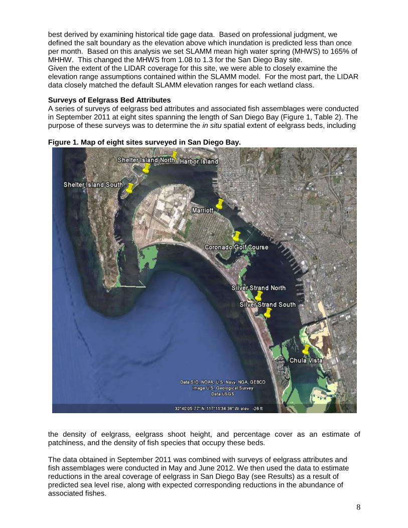
Surveys of Eelgrass Bed Attributes A series of surveys of eelgrass bed attributes and associated fish assemblages were conducted in September 2011 at eight sites spanning the length of San Diego Bay (Figure 1, Table 2). The purpose of these surveys was to determine the in situ spatial extent of eelgrass beds, including Figure 1. Map of eight sites surveyed in San Diego Bay.

the density of eelgrass, eelgrass shoot height, and percentage cover as an estimate of patchiness, and the density of fish species that occupy these beds. The data obtained in September 2011 was combined with surveys of eelgrass attributes and fish assemblages were conducted in May and June 2012. We then used the data to estimate reductions in the areal coverage of eelgrass in San Diego Bay (see Results) as a result of predicted sea level rise, along with expected corresponding reductions in the abundance of associated fishes.

9

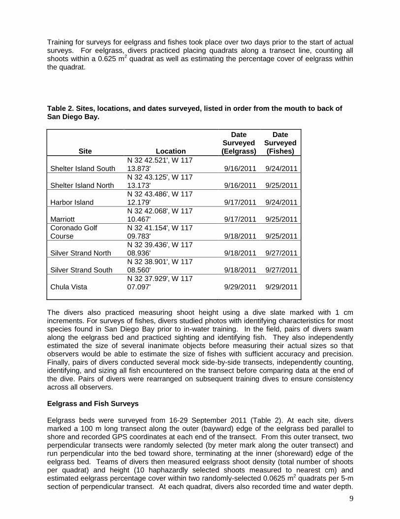
Training for surveys for eelgrass and fishes took place over two days prior to the start of actual surveys. For eelgrass, divers practiced placing quadrats along a transect line, counting all shoots within a 0.625 m2 quadrat as well as estimating the percentage cover of eelgrass within the quadrat. Table 2. Sites, locations, and dates surveyed, listed in order from the mouth to back of San Diego Bay.

Site Location

Date Surveyed (Eelgrass)

Date Surveyed (Fishes)

Shelter Island South N 32 42.521', W 117 13.873' 9/16/2011 9/24/2011

Shelter Island North N 32 43.125', W 117 13.173' 9/16/2011 9/25/2011

Harbor Island N 32 43.486', W 117 12.179' 9/17/2011 9/24/2011

Marriott N 32 42.068', W 117 10.467' 9/17/2011 9/25/2011

Coronado Golf Course

N 32 41.154', W 117 09.783' 9/18/2011 9/25/2011

Silver Strand North N 32 39.436', W 117 08.936' 9/18/2011 9/27/2011

Silver Strand South N 32 38.901', W 117 08.560' 9/18/2011 9/27/2011

Chula Vista N 32 37.929', W 117 07.097' 9/29/2011 9/29/2011

The divers also practiced measuring shoot height using a dive slate marked with 1 cm increments. For surveys of fishes, divers studied photos with identifying characteristics for most species found in San Diego Bay prior to in-water training. In the field, pairs of divers swam along the eelgrass bed and practiced sighting and identifying fish. They also independently estimated the size of several inanimate objects before measuring their actual sizes so that observers would be able to estimate the size of fishes with sufficient accuracy and precision. Finally, pairs of divers conducted several mock side-by-side transects, independently counting, identifying, and sizing all fish encountered on the transect before comparing data at the end of the dive. Pairs of divers were rearranged on subsequent training dives to ensure consistency across all observers. Eelgrass and Fish Surveys Eelgrass beds were surveyed from 16-29 September 2011 (Table 2). At each site, divers marked a 100 m long transect along the outer (bayward) edge of the eelgrass bed parallel to shore and recorded GPS coordinates at each end of the transect. From this outer transect, two perpendicular transects were randomly selected (by meter mark along the outer transect) and run perpendicular into the bed toward shore, terminating at the inner (shoreward) edge of the eelgrass bed. Teams of divers then measured eelgrass shoot density (total number of shoots per quadrat) and height (10 haphazardly selected shoots measured to nearest cm) and estimated eelgrass percentage cover within two randomly-selected 0.0625 m2 quadrats per 5-m section of perpendicular transect. At each quadrat, divers also recorded time and water depth.

10

Finally, one diver recorded the depth and time of the outer edge of the eelgrass bed every 5 m along the outer transect, measured perpendicular to the transect at each point if the actual bed edge deviated from the transect line. Fish surveys were conducted from 24-29 September 2011 (Table 2). Divers placed a transect line perpendicular to shore from the outer edge of the eelgrass bed to the inner edge. The transect line was located between and roughly equidistant from the two GPS coordinates marking the ends of the 100 m eelgrass survey outer transect to ensure that the same portion of the bed was surveyed. Four 30 m x 2 m wide x 2 m high transects (120 m3) were surveyed at each of three strata within the eelgrass bed: the outer edge, middle of the bed (location estimated by halving the bed width along the perpendicular transect), and inner edge. Divers began at the perpendicular transect and swam parallel to shore at a slow to moderate pace while counting, identifying, and visually estimating the size of all fishes in the transect area. At the end of this first transect, the divers then swam an additional 10 m before beginning the second transect to avoid sampling the same area or the same individual fish. After completing two transects the divers returned to the perpendicular transect and repeated the procedure, conducting two transects in the other direction parallel to shore. For each transect, divers noted the depth and water temperature, estimated the percentage cover of eelgrass along the entire transect, and qualitatively described current speed (low, moderate, or high). Water visibility was also measured as the farthest distance from which the diver was able to discern the ridged texture of the rebar stake used to hold the transect lines in place. Due to the often low visibility (1.5 m or less), demersal fish were occasionally encountered but swam out of sight before they could be identified or sized, leaving a cloud of sediment behind. Divers therefore also counted the frequency of these sediment clouds on each transect. RESULTS Original San Diego Bay Digital Terrain Model Mosaic A seamless bathymetric/topographic digital elevation model (DEM) was first developed in this project for San Diego Bay (Figure 2) .The gridding and merging of the bathymetric and topographic data were accomplished using the data conversion, buffering, clipping, interpolation, mosaicking, and smoothing tools available in the ArcInfo GIS package. The resulting merged bathymetric/topographic model was output in the ArcInfo GRID format.

11

Figure 2. The Seamless San Diego Bay Digital Terrain Model Mosaic

12

Updated San Diego Bay Digital Terrain Model Mosaic An updated seamless bathymetric/topographic digital elevation model (DEM) was first developed in this project for San Diego Bay using the LiDAR DEM that we had generated from 2006 LiDAR flights by the City of San Diego. This was then coupled with existing bathymetry developed for the San Diego Unified Port District. However in 2012, a new LiDAR DEM was made available from LiDAR data for 2009-2011 by NOAA (Digital Coast, Coastal LiDAR Project). So we next replaced the original 2006 LiDAR flight for the City of San Diego by the new NOAAA LiDAR DEM. This hydro-flattened surface was then merged seamlessly with the bathymetry The latest high resolution bathymetry data generated by Dr. Neal Driscoll at Scripps Institute of Oceanography was also used in this updated DEM. The 7 ASCII files for the Scripps bathymetry have been merged into a single grid with a 1-meter resolution. This grid was projected from the WGS84 coordinate space into the UTM NAD83 coordinate space. We first converted the bathymetry data into ArcGIS format, smoothed the data to remove sinks and peaks and QA/QC’d the data, and then merged/mosaicked the bathymetry tiles. We next processed the data for gaps in the bathymetry (shallow areas and the South Bay) and then merged the bathymetry with the NOAA Digital Coast LiDAR data to produce the seamless terrain model (Figure 3).

13

Figure 3. The area within the blue boundary on the PDF is the area of extent for the Scripps bathymetry of Dr. Driscoll.The grey area inside the black line on the map is the 2008 bathymetry from the Port District merged into Dr. Driscoll’s bathymetry.

14

SLAMM Modeling of San Diego Bay We first delineated (with the help of Eileen Maher of Port Staff) the specific wetlands that are under the jurisdiction of the San Diego Unified Port District (Figure 4). We then modeled the changes in each of the coastal wetland habitats delineated in Figure 3.These alterations were modeled by SLAMM to yield a prediction of habitat alteration by the year 2100 assuming a 2 meter sea level rise. Tables 3-8 show the habitat change for each of these Port’s jurisdictional sites assuming a 2m sea level rise by 2100. Table 9 shows the change in habitat under the 2 meter sea level rise scenario (as compared to the present) for the total area of coastal wetlands under the jurisdiction of the Port District. Our modeling results show that salt marsh (and brackish marsh) will decline by nearly 90% under the sea level rise scenario used (2 meter rise). This will have significant implications on habitat loss and preservation of certain sensitive/endangered species in the future. Table 3. Modeled habitat alteration of Port jurisdictional site #1 (refer to map on Figure 4). Blue color represents increase in habitat area, and red a decrease in habitat area by 2100.

Name VALUE_ COUNT_ Square meters

hectares Initial coverage(%)

Hectares in 2100 @ 2m)

Percent Change

Developed dryland

1 8 800 0.08 3.56 0.08 0

Undeveloped dryland

2 1 100 0.01 0.44 0 -100

Saltmarsh 8 165 16500 1.65 73.33 1.65 0

Estuarine beach

10 13 1300 0.13 5.78 0.14 7.7

Brackish marsh

20 38 3800 0.38 16.89 0.38 0

Total 225 22500 2.25 100 2.25

Table 4. Modeled habitat alteration of Port jurisdictional site #2 (refer to map on Figure 4). Blue color represents increase in habitat area, and red a decrease in habitat area by 2100.

Name VALUE_ COUNT_ square meters

hectares Initial coverage (%)

hectares in 2100 @2m

Percent change (%)

Developed dryland

1 29 2900 0.29 19.73 0.29 0

Undeveloped Dryland

2 23 2300 0.23 15.65 0 -100

Saltmarsh 8 57 5700 0.57 38.78 0.01 -98.2

Estuarine Beach 10 38 3800 0.38 25.85 0.22 -42.1

Tidal Flat 11 0 0 0 0.00 0.01 na

Estuarine Openwater

17 0 0 0 0.00 0.94 na

Total 14700 1.47 100.00 1.47

15

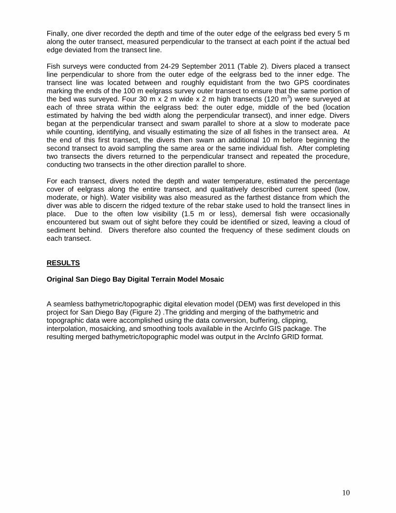
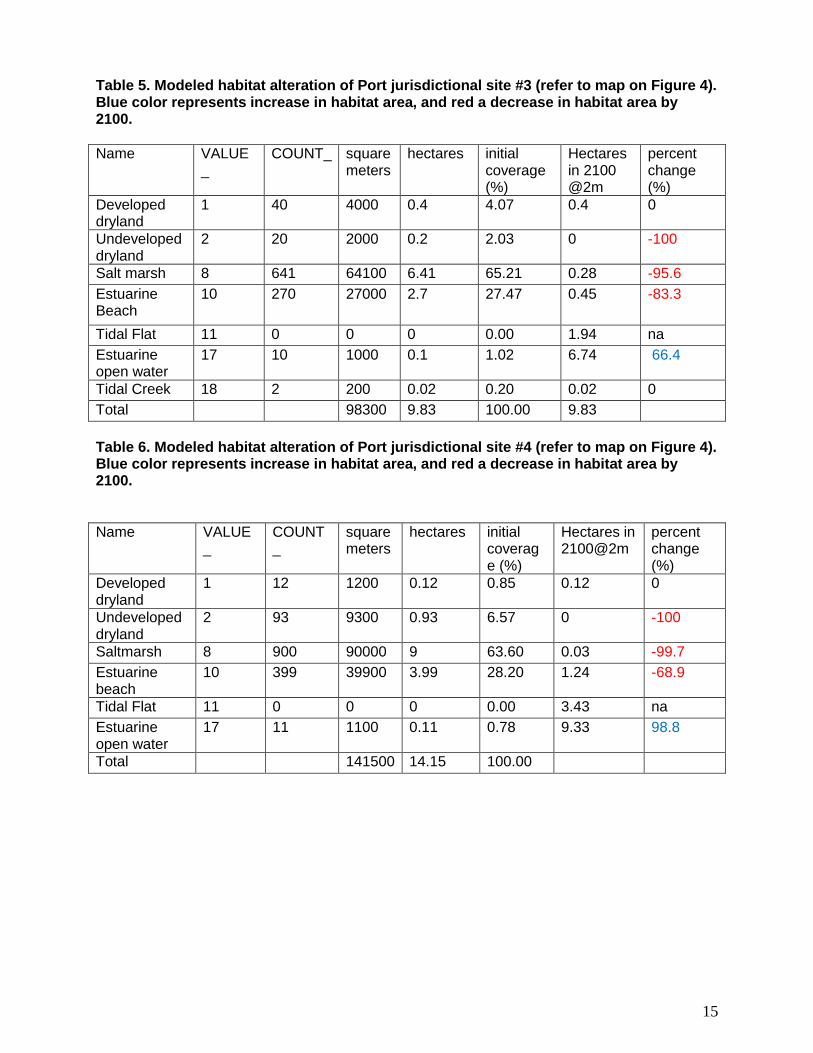
Table 5. Modeled habitat alteration of Port jurisdictional site #3 (refer to map on Figure 4). Blue color represents increase in habitat area, and red a decrease in habitat area by 2100.

Name VALUE_

COUNT_ square meters

hectares initial coverage (%)

Hectares in 2100 @2m

percent change (%)

Developed dryland

1 40 4000 0.4 4.07 0.4 0

Undeveloped dryland

2 20 2000 0.2 2.03 0 -100

Salt marsh 8 641 64100 6.41 65.21 0.28 -95.6

Estuarine Beach

10 270 27000 2.7 27.47 0.45 -83.3

Tidal Flat 11 0 0 0 0.00 1.94 na

Estuarine open water

17 10 1000 0.1 1.02 6.74 66.4

Tidal Creek 18 2 200 0.02 0.20 0.02 0

Total 98300 9.83 100.00 9.83

Table 6. Modeled habitat alteration of Port jurisdictional site #4 (refer to map on Figure 4). Blue color represents increase in habitat area, and red a decrease in habitat area by 2100.

Name VALUE_

COUNT_

square meters

hectares initial coverage (%)

Hectares in 2100@2m

percent change (%)

Developed dryland

1 12 1200 0.12 0.85 0.12 0

Undeveloped dryland

2 93 9300 0.93 6.57 0 -100

Saltmarsh 8 900 90000 9 63.60 0.03 -99.7

Estuarine beach

10 399 39900 3.99 28.20 1.24 -68.9

Tidal Flat 11 0 0 0 0.00 3.43 na

Estuarine open water

17 11 1100 0.11 0.78 9.33 98.8

Total 141500 14.15 100.00

16

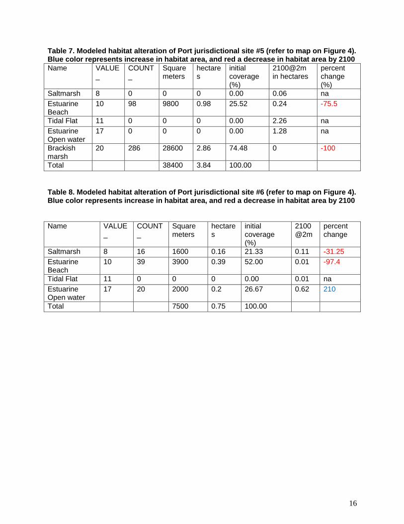
Table 7. Modeled habitat alteration of Port jurisdictional site #5 (refer to map on Figure 4). Blue color represents increase in habitat area, and red a decrease in habitat area by 2100

Name VALUE_

COUNT_

Square meters

hectares

initial coverage (%)

2100@2m in hectares

percent change (%)

Saltmarsh 8 0 0 0 0.00 0.06 na

Estuarine Beach

10 98 9800 0.98 25.52 0.24 -75.5

Tidal Flat 11 0 0 0 0.00 2.26 na

Estuarine Open water

17 0 0 0 0.00 1.28 na

Brackish marsh

20 286 28600 2.86 74.48 0 -100

Total 38400 3.84 100.00

Table 8. Modeled habitat alteration of Port jurisdictional site #6 (refer to map on Figure 4). Blue color represents increase in habitat area, and red a decrease in habitat area by 2100

Name VALUE_

COUNT_

Square meters

hectares

initial coverage (%)

2100 @2m

percent change

Saltmarsh 8 16 1600 0.16 21.33 0.11 -31.25

Estuarine Beach

10 39 3900 0.39 52.00 0.01 -97.4

Tidal Flat 11 0 0 0 0.00 0.01 na

Estuarine Open water

17 20 2000 0.2 26.67 0.62 210

Total 7500 0.75 100.00

17

Figure 4. Coastal wetlands (numbered #1 through #6) under the jurrisdiction of the San Diego Unified Port District.

18

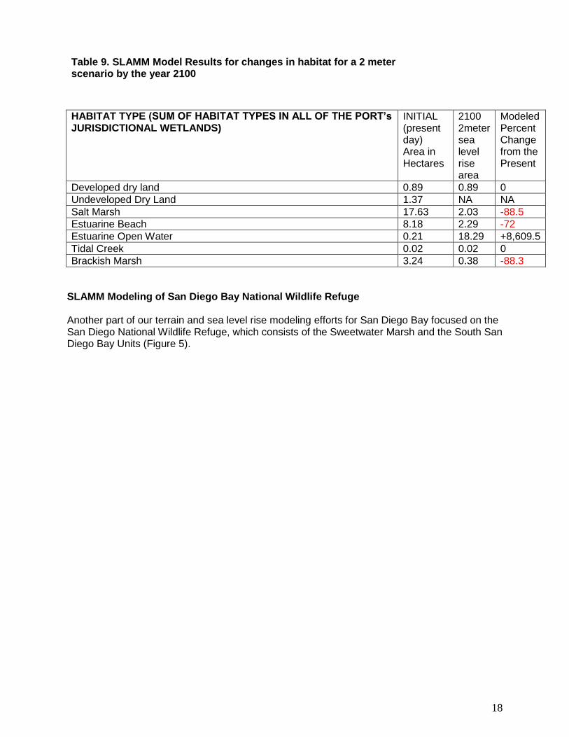
Table 9. SLAMM Model Results for changes in habitat for a 2 meter sea level rise scenario by the year 2100

HABITAT TYPE (SUM OF HABITAT TYPES IN ALL OF THE PORT’s JURISDICTIONAL WETLANDS)

INITIAL (present day) Area in Hectares

2100 2meter sea level rise area

Modeled Percent Change from the Present

Developed dry land 0.89 0.89 0

Undeveloped Dry Land 1.37 NA NA

Salt Marsh 17.63 2.03 -88.5

Estuarine Beach 8.18 2.29 -72

Estuarine Open Water 0.21 18.29 +8,609.5

Tidal Creek 0.02 0.02 0

Brackish Marsh 3.24 0.38 -88.3

SLAMM Modeling of San Diego Bay National Wildlife Refuge Another part of our terrain and sea level rise modeling efforts for San Diego Bay focused on the San Diego National Wildlife Refuge, which consists of the Sweetwater Marsh and the South San Diego Bay Units (Figure 5).

19

Figure 5. San Diego Bay National Wildlife Refuge

20

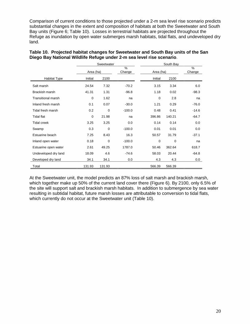
Comparison of current conditions to those projected under a 2-m sea level rise scenario predicts substantial changes in the extent and composition of habitats at both the Sweetwater and South Bay units (Figure 6; Table 10). Losses in terrestrial habitats are projected throughout the Refuge as inundation by open water submerges marsh habitats, tidal flats, and undeveloped dry land. Table 10. Projected habitat changes for Sweetwater and South Bay units of the San Diego Bay National Wildlife Refuge under 2-m sea level rise scenario.

Sweetwater

South Bay

Area (ha)

% Change

Area (ha)

% Change

Habitat Type Initial 2100

Initial 2100

Salt marsh 24.54 7.32

-70.2

3.15 3.34

6.0

Brackish marsh 41.31 1.31

-96.8

1.18 0.02

-98.3

Transitional marsh 0 1.62

na

0 2.8

na

Inland fresh marsh 0.1 0.07

-30.0

1.21 0.29

-76.0

Tidal fresh marsh 0.2 0

-100.0

0.48 0.41

-14.6

Tidal flat 0 21.98

na

396.86 140.21

-64.7

Tidal creek 3.25 3.25

0.0

0.14 0.14

0.0

Swamp 0.3 0

-100.0

0.01 0.01

0.0

Estuarine beach 7.25 8.43

16.3

50.57 31.79

-37.1

Inland open water 0.18 0

-100.0

0 0

na

Estuarine open water 2.61 49.25

1787.0

50.46 362.64

618.7

Undeveloped dry land 18.09 4.6

-74.6

58.03 20.44

-64.8

Developed dry land 34.1 34.1 0.0 4.3 4.3 0.0

Total 131.93 131.93 566.39 566.39

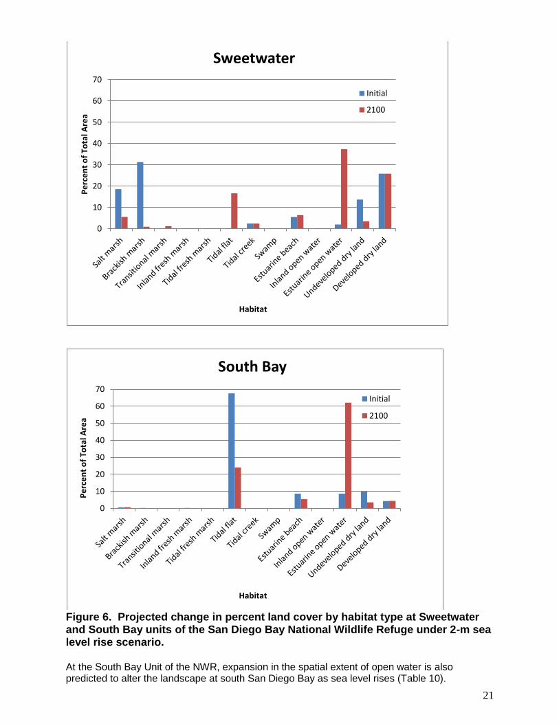
At the Sweetwater unit, the model predicts an 87% loss of salt marsh and brackish marsh, which together make up 50% of the current land cover there (Figure 6). By 2100, only 6.5% of the site will support salt and brackish marsh habitats. In addition to submergence by sea water resulting in subtidal habitat, future marsh losses are attributable to conversion to tidal flats, which currently do not occur at the Sweetwater unit (Table 10).

21

Figure 6. Projected change in percent land cover by habitat type at Sweetwater and South Bay units of the San Diego Bay National Wildlife Refuge under 2-m sea level rise scenario. At the South Bay Unit of the NWR, expansion in the spatial extent of open water is also predicted to alter the landscape at south San Diego Bay as sea level rises (Table 10).

0

10

20

30

40

50

60

70P

erc

en

t o

f To

tal A

rea

Habitat

Sweetwater

Initial

2100

0

10

20

30

40

50

60

70

Pe

rce

nt

of

Tota

l Are

a

Habitat

South Bay

Initial

2100

22

Currently, open water makes up less than 9% of the land cover, but by 2100 will make up 62%. Sea water will submerge large expanses of tidal flats, which cover nearly 70% of the site currently, and will reduce cover of this habitat type to 24% by 2100 (Figure 6). Effect of Sea Level Rise on Eelgrass Habitat in San Diego Bay Results of Eelgrass and Fish Assemblage Survey All data from the fall 2011 led to estimates of eelgrass attributes (Table 11) and densities of fishes (Table 12) have been compiled by site. These data were combined with data obtained from spring 2012 surveys that will take place to provide estimates of the spatial extent of eelgrass beds, eelgrass parameters (shoot density, shoot height, and percentage cover), and the density and biomass of fishes. To determine fish biomass, estimated lengths of fish will be converted to biomass using established length-weight regressions in reports and publications from existing literature. Table 11. Eelgrass shoot density, percentage cover, and shoot height among sites in San Diego Bay, with respective standard deviations (± 1 Std. Dev.).

Site Shoot

density SD % cover SD Shoot height SD

Shelter Island South 67.3 46.0 33.7 29.7 46.5 16.4 Shelter Island North 48.5 66.3 24.2 15.3 31.6 18.6 Harbor Island 31.8 32.1 15.7 22.5 46.5 18.4 Marriott 410.9 283.3 53.6 38.4 26.0 6.0 Coronado Golf Course 163.1 158.7 46.7 37.0 27.6 10.4 Silver Strand North 48.1 66.0 27.2 36.0 29.6 15.6 Silver Strand South 17.3 44.1 7.2 17.1 24.4 11.4 Chula Vista 76.5 43.7 33.2 23.8 31.9 8.0

Table 12. Numerical densities (no. / 500 m3) of seven common fishes among sites in San Diego Bay.

Site Round

ray Spotted

bass Kelp bass

Black surfperch

Shiner surfperch

Giant kelpfish Silversides

Shelter Island South 0 1.7 4.9 25.7 15.6 3.1 81.3 Shelter Island North 5.9 3.8 0 0 0 3.1 81.6 Harbor Island 2.1 1.7 5.9 5.9 0.7 4.5 45.1 Marriott 2.8 1.7 0.0 0.3 0 3.5 3.5 Coronado Golf Course 7.3 2.4 0 0 0 9.4 0 Silver Strand North 2.8 0.7 0 0 0 0 0 Silver Strand South 1.7 0.3 0 0 0 0 0 Chula Vista 6.3 4.5 0 0 0 0 0

23

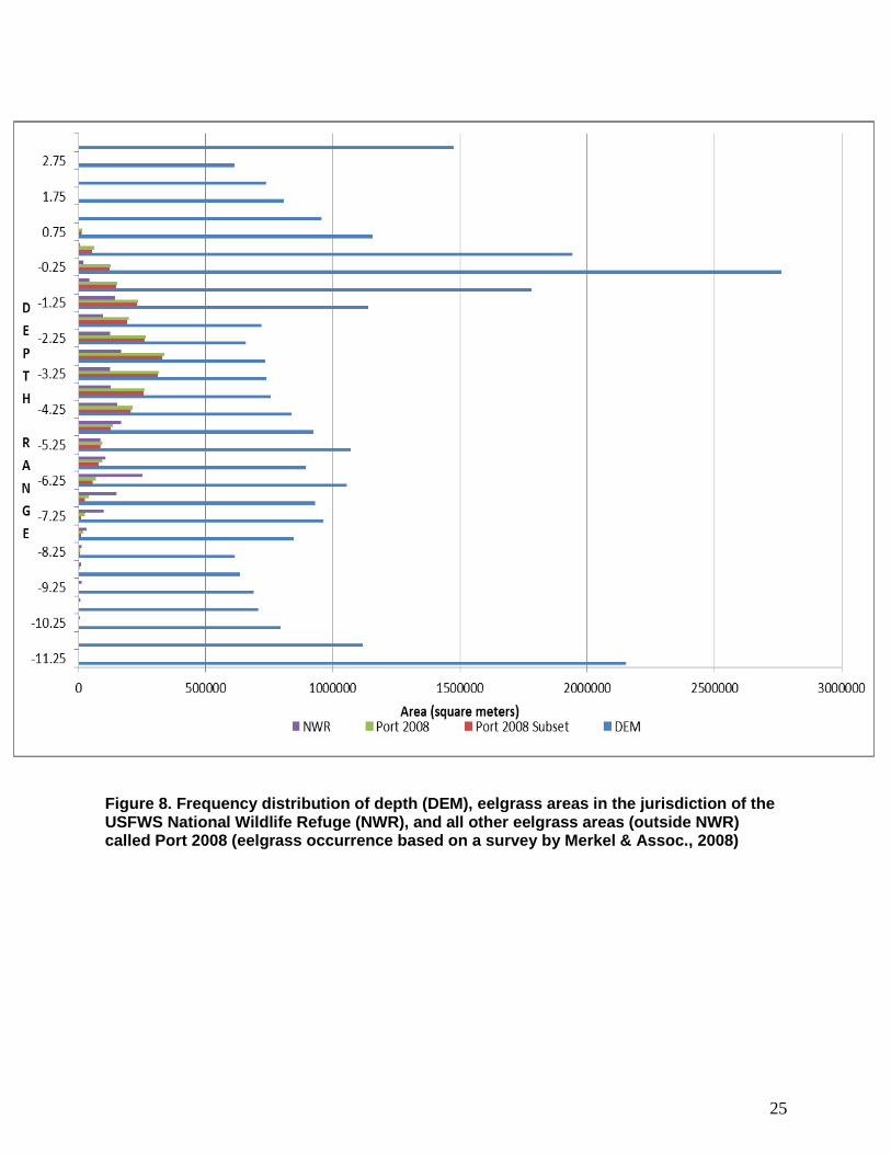
Figure 7 shows a graphic of the eelgrass areas in San Diego Bay draped onto our terrain model for San Diego Bay that were modeled for our analysis. The terrain model is symbolized with the elevation ranges (in feet of water depth) by frequency distributions of eelgrass occurrence in Figures 8 and 9. Shown on these Figures are the frequency distributions of depth (DEM), eelgrass areas in the jurisdiction of the USFWS National Wildlife Refuge (NWR), and all other eelgrass areas (outside NWR) called Port 2008 (eelgrass occurrence based on a survey for the San Diego Unified Port District done by Merkel & Assoc., 2008). It can be seen from Figure 8 that the most frequent depth in south Saqn Diego Bay is between 3.75-4.75 feet. Furthermore, the most frequent depth of eelgrass occurrence within the National Wildlife Refuge is about the same (3.75-4.75 ft.), while the most frequent depth for all other eelgrass areas (Port 2008) in south San Diego Bay is shallower (between 1.75-2.75 feet).

24

Figure 7. Eelgrass occurrence draped onto the San Diego Bay terrain model

25

Figure 8. Frequency distribution of depth (DEM), eelgrass areas in the jurisdiction of the USFWS National Wildlife Refuge (NWR), and all other eelgrass areas (outside NWR) called Port 2008 (eelgrass occurrence based on a survey by Merkel & Assoc., 2008)

26

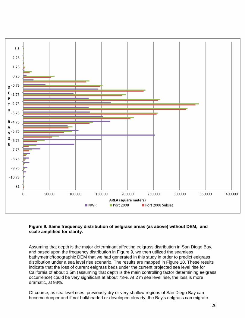
Figure 9. Same frequency distribution of eelgrass areas (as above) without DEM, and scale amplified for clarity. Assuming that depth is the major determinant affecting eelgrass distribution in San Diego Bay, and based upon the frequency distribution in Figure 9, we then utilized the seamless bathymetric/topographic DEM that we had generated in this study in order to predict eelgrass distribution under a sea level rise scenario. The results are mapped in Figure 10. These results indicate that the loss of current eelgrass beds under the current projected sea level rise for California of about 1.5m (assuming that depth is the main controlling factor determining eelgrass occurrence) could be very significant at about 73%. At 2 m sea level rise, the loss is more dramatic, at 93%. Of course, as sea level rises, previously dry or very shallow regions of San Diego Bay can become deeper and if not bulkheaded or developed already, the Bay’s eelgrass can migrate

0 50000 100000 150000 200000 250000 300000 350000 400000

-31

-10.75

-9.75

-8.75

-7.75

-6.75

-5.75

-4.75

-3.75

-2.75

-1.75

-0.75

0.25

1.25

2.25

3.5

AREA (square meters)

D

E

P

T

H

R

A

N

G

E

NWR Port 2008 Port 2008 Subset

27

inland to these new areas. We next used the seamless model to estimate areas for potential migration of eelgrass under sea level rise scenarios.

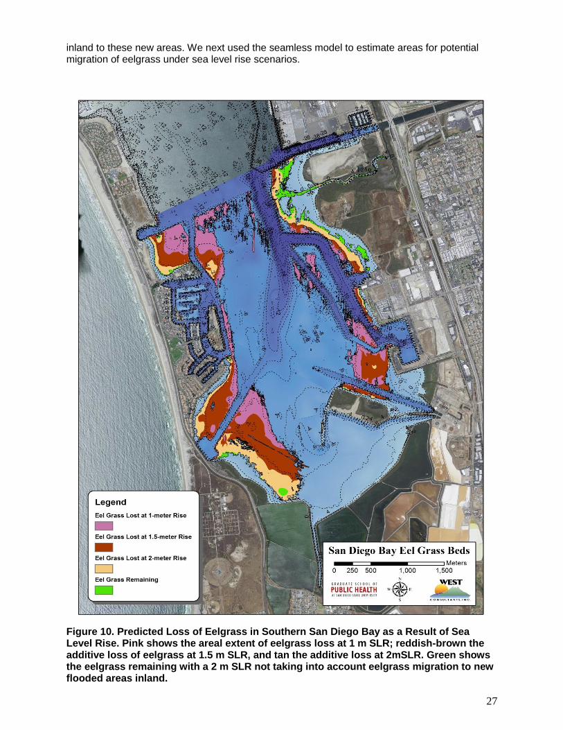
Figure 10. Predicted Loss of Eelgrass in Southern San Diego Bay as a Result of Sea Level Rise. Pink shows the areal extent of eelgrass loss at 1 m SLR; reddish-brown the additive loss of eelgrass at 1.5 m SLR, and tan the additive loss at 2mSLR. Green shows the eelgrass remaining with a 2 m SLR not taking into account eelgrass migration to new flooded areas inland.

28

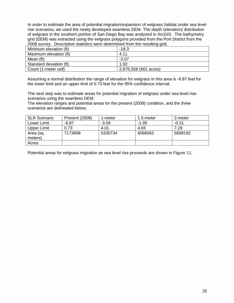
In order to estimate the area of potential migration/expansion of eelgrass habitat under sea level rise scenarios, we used the newly developed seamless DEM. The depth (elevation) distribution of eelgrass in the southern portion of San Diego Bay was analyzed in ArcGIS. The bathymetry grid (DEM) was extracted using the eelgrass polygons provided from the Port District from the 2008 survey. Descriptive statistics were determined from the resulting grid.

Minimum elevation (ft) -18.3

Maximum elevation (ft) 4.11

Mean (ft) -3.07

Standard deviation (ft) 1.92

Count (1-meter cell) 2,675,558 (661 acres)

Assuming a normal distribution the range of elevation for eelgrass in this area is -6.87 feet for the lower limit and an upper limit of 0.73 feet for the 95% confidence interval. The next step was to estimate areas for potential migration of eelgrass under sea level rise scenarios using the seamless DEM. The elevation ranges and potential areas for the present (2008) condition, and the three scenarios are delineated below:

SLR Scenario Present (2008) 1-meter 1.5-meter 2-meter

Lower Limit -6.87 -3.59 -1.95 -0.31

Upper Limit 0.73 4.01 4.65 7.29

Area (sq. meters)

7173698 5335734 6068562 5699192

Acres

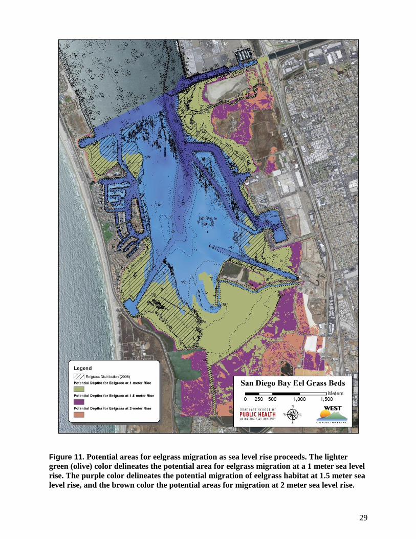
Potential areas for eelgrass migration as sea level rise proceeds are shown in Figure 11.

29

Figure 11. Potential areas for eelgrass migration as sea level rise proceeds. The lighter

green (olive) color delineates the potential area for eelgrass migration at a 1 meter sea level

rise. The purple color delineates the potential migration of eelgrass habitat at 1.5 meter sea

level rise, and the brown color the potential areas for migration at 2 meter sea level rise.

30

DISCUSSION The development of an updated high resolution and seamless San Diego Bay bathymetic/topographic model (also known as digital terrain model) (Figure 3), has resulted in a prototype digital product that that can be employed for San Diego Bay GIS and coastal zone management applications. It demonstrates how disparate spatial data can be utilized together if they are first transformed to a common reference coordinate system. This is the first up-to-date merged seamless elevation model whose use as a base data layer facilitates overlay and incorporation of other spatially referenced coastal and marine datasets. The base DEM can easily be converted to support mapping and other GIS applications, enhanced for data visualization, used for input to 2-D and 3-D environmental models, and employed in a predictive fashion to model the habitat (as we have done for coastal wetlands and eelgrass) and infrastructure effects of sea level rise. Additionally, we used this digital terrain model of San Diego Bay to predict the changes in each of the coastal wetland habitats delineated in Figure 4 that are under the jurisdiction of the Port District. These wetlands were modeled by SLAMM to yield a prediction of habitat alteration by the year 2100 assuming a 2 meter sea level rise. Table 9 shows the change in habitat under the 2 meter sea level rise scenario (as compared to the present) for the total area of coastal wetlands under the jurisdiction of the Port. Our modeling results show that salt marsh (and brackish marsh) will decline by nearly 90% under the sea level rise scenario used (2 meter rise). This will have significant implications on habitat loss and preservation of certain sensitive/endangered species in the future. We also used SLAMM to model the changes to the San Diego Bay National Wildlife Refuge with sea level rise. This Refuge is situated at the south end of San Diego Bay, and is surrounded by urban development within the Cities of National City, Chula Vista, San Diego, Imperial Beach and Coronado. The Refuge encompasses approximately 2,620 acres of land and water in and around San Diego Bay. The 316 acre Sweetwater Marsh supports tidally influenced salt marsh habitat, disturbed upland habitat and the D street Fill, an old dredge disposal site that provides nesting habitat for terns and western snowy plovers (USFWS, 2006). However the most significant habitat on this Refuge Unit is coastal salt marsh. This habitat supports the Federally-endangered light-footed clapper rail, and the state endangered Belding’s savannah sparrow. The clapper rail depends almost entirely on salt marsh habitat for feeding and nesting. Belding’s savannah sparrow is found throughout the salt marsh area of this Refuge unit, and forage within salt marsh and intertidal mudflat habitat. The South San Diego Bay Unit currently includes about 2,300 acres including portions of open bay (eelgrass habitat), salt ponds, and the Otay River floodplain. The saltponds provide resting and foraging habitat for a wide variety of avian species, while the levees are important nesting habitat for seven species of ground nesting seabirds. Eelgrass beds in the subtidal habitat of the South San Diego Bay Unit provide highly productive microhabitats for a variety of invertebrates and fish. San Diego Bay’s population of green sea turtles also relies on eelgrass as an important food source. Our model predicts declines in several species of conservation concern by the end of the 21st century. At the Sweetwater unit, the model predicts an 87% loss of salt marsh and brackish marsh, which together make up 50% of the current land cover there (Figure 6). By 2100, only 6.5% of the site will support salt and brackish marsh habitats. At the South Bay Unit of the NWR, expansion in the spatial extent of open water is also predicted to alter the landscape at south San Diego Bay as sea level rises (Table 10). However, it is likely that habitat declines will occur sooner than the permanent loss of their preferred habitats. As global climate changes, predictions are that tidal range may increase

31

faster than mean sea level, increasing the frequency and duration of extreme high tides that cause over-marsh flooding (Takekawa et al. 2006). Prolonged marsh inundation could increase nest mortality for marsh nesting species, and make marshes unavailable for foraging and roosting, forcing birds into uplands where they may be more vulnerable to predators and may experience inferior feeding conditions Sea-level rise will have a variety of effects on eelgrass habitat. Increased water depth will restrict the amount of light reaching eelgrasses, and depending on the bathymetry of the Bay and topography of the surrounding landscape, change the geographic distribution of the eelgrass habitat. In addition, changes in tidal dynamics (e.g., water current speed, circulation flow patterns, tidal range) could have a range of impacts including reductions in light, an increase in water column turbidity, and alterations of the temperature regime. Based upon our current understanding of eelgrass distribution, it does indeed seem likely that sea level rise will move the maximum depth of eelgrass growth and abundance closer to the current shoreline. The aim of the current effort is to use the seamless San Diego Bay Digital Elevation Model to better quantify this impact of sea level rise. Our modeling using the seamless bathymetric/topographic DEM that we have generated shows future alteration of eelgrass beds that are mapped on the attached Figure 10. These results indicate that assuming depth is the major determinant affecting eelgrass distribution in San Diego Bay, then the loss of current eelgrass beds under the current projected sea level rise for California of about 1.5m (assuming that depth is the main controlling factor determining eelgrass occurrence) could be very significant at about 73%. At 2 m sea level rise, the loss is more dramatic, at 93%. Sea level rise and its effects will have profound implications for both the coastal habitats (coastal wetlands and eelgrass beds) of San Diego Bay as well as the surrounding human communities and their infrastructure. We have used our main product of this project- the seamless bathymetric/digital elevation model of San Diego Bay to predict the future changes to the coastal habitats. Our models now predict major losses in habitat of both saltmarsh and eelgrass, so with this in mind it is imperative that steps are taken to safeguard if possible, and mitigate in these low-lying coastal ecosystems against the worst impacts of sea level rise, not just for wildlife, but also for human societies. REFERENCES

Cahoon, D. R., J. C. Lynch, and A. N. Powell. 1996. Marsh vertical accretion in a southern California estuary, U.S.A. Estuarine, Coastal and Shelf Science 43:19-32.

Clough, J.S. and R.A. Park, 2007, Technical Documentation for SLAMM 5.0.1 February 2008, Jonathan S. Clough, Warren Pinnacle Consulting, Inc, Richard A. Park, Eco Modeling. http://warrenpinnacle.com/prof/SLAMM

IPCC. 2013. Climate Change 2013: Fifth Assessment Report. Intergovernmental Panel on Climate Change.

Merkel & Assoc. 2008. San Diego Bay Eelgrass Survey. Conducted in cooperation with Naval Facilities Engineering Command Southwest Natural Resources and Port of San Diego.

32

Nicholls, R.J., Marinova, N., Lowe, J., Brown, S., Vellinga, P., de Gusmao, D., Hinkel, J. and R. S.J. Tol. 2010 Sea-level rise and its possible impacts given a ‘beyond 4°C world’ in the twenty-first. Phil. Trans. of Royal Soc. http://dx.doi.org/10.1098/rsta.2010.0291

Pfeffer, Harper, O'Neel, 2008. Kinematic Constraints on Glacier Contributions to 21st-Century Sea-Level Rise. Science, Vol. 321, No. 5894. (5 September 2008), pp. 1340-134

Rahmstorf, Stefan 2007, “A Semi-Empirical Approach to Projecting Future Sea-Level Rise,” Science 2007 315: 368-370.

Rohling, E.J, Grant, K., Hemleben, Ch., Siddall, M., Hoogakker, B.A.A., Bolshaw, M.and M. Kucera. 2008. High rates of sea-level rise during the last interglacial period Nat. Geosci. 1: 38–42

Takekawa, J. Y., I. Woo, H. Spautz, N. Nur, J. L. Grenier, K. Malamud-Roam, J. J. Nordby, An N. Cohen, F. Malamud-Roam, and S. E. Wainwright-de la Cruz. 2006. Environmental threats to tidal-marsh vertebrates of the San Francisco Bay Estuary. Studies in Avian Biology 32:176-197.

Thum, Alan, PhD, Gibson, Doug, Laton, Richard, and Foster, John. 2000.Sediment Quality And Depositional Environment Of San Elijo Lagoon, Technical Report Prepared for: Coastal Conservancy and U.S. Fish & Wildlife Service.

Vermeer, M. and S. Rahmstorf. 2009. PNAS Global sea level linked to global temperature. Proc. Nat. Acad. Sci. 106: 21527-21532.

Weis, D. A., Callaway, A. B. and Gersberg, R. M., 2001.Vertical accretion rates and heavy metal chronologies in wetland sediments of the Tijuana Estuary. Estuaries, 24(6A), 840-850.