SAN DIEGO RIVER WATERSHED MONITORING AND …

SAN DIEGO RIVER WATERSHED MONITORING AND ASSESSMENT PROGRAM

Submitted to the

San Diego Regional Water Quality Control Board

by

Brock B. Bernstein

January 20, 2014

April 9, 2014 Item No. 6

Supporting Document No. 4

Acknowledgments This project was funded by the San Diego Regional Water Quality Control Board (SRWQCB) using regional Surface Water Ambient Monitoring Program (SWAMP) funds. The content of the report was contributed over the course of 2011 – 2013 by a workgroup consisting of regulated, regulatory, environmental, and research organizations. Members who participated for all or part of this effort included: Agency

Staff

California Department of Fish and Wildlife Russell Barabe Bryand Duke Peter Ode Paul Schlitt California Department of Transportation May Alsheikh Ken Johansson Constantine Kontaxis City of El Cajon Jaime Campos City of San Diego Ruth Kolb Jeff Pasek Andre Sonksen City of Santee Helen Davies Julie Procopio Cleveland National Forest Jason Jimenez EcoLayers Clay Clifton Joe Purohit Facilitator Brock Bernstein Helix Water District Mark Umphres Padre Dam Municipal Water District Gary Canfield Arne Sandvik San Diego Coastkeeper Travis Pritchard San Diego County Steven DiDonna Stephanie Gaines Jo Ann Weber San Diego Regional Water Quality Control Board Christine Arias Lilian Busse Jody Ebsen Cynthia Gorham Cathryn Henning

Carey Nagoda Chad Loflen

Bruce Posthumus Barry Pulver Deborah Woodward San Diego River Conservancy Mike Nelson San Diego River Park Foundation Shannon Quigley-Raymond

Gary Strawn San Diego State University Matt Rahn San Diego Stream Team Bob Stafford



Southern California Coastal Water Research Project Eric Stein Martha Sutula Tijuana National Estuarine Research Reserve Jeff Crooks TRL Jerome Jaminet US Army Corps of Engineers Peggy Bartels US Geological Survey Greg Mendez In addition to these workgroup members, invited experts provided valuable information and advice on a number of key issues.



Table of Contents Acknowledgments .......................................................................................................................................... i Executive Summary ...................................................................................................................................... v

1.0 Introduction ............................................................................................................................................. 1

1.1 Background ......................................................................................................................................... 1

1.2 Workgroup approach .......................................................................................................................... 2

1.3 Implementation ................................................................................................................................... 2

1.4 Regional setting .................................................................................................................................. 3

2.0 Watershed Boundaries and Management Questions ............................................................................... 7

2.1Boundaries of the watershed ................................................................................................................ 7

2.2 Key management questions ................................................................................................................ 7

2.3.1 Beneficial uses ............................................................................................................................. 7

2.3.2 Management questions ................................................................................................................. 7

2.3 Watershed report card ......................................................................................................................... 8

3.0 Watershed Report Card ......................................................................................................................... 12

3.1. Need for a watershed report card ..................................................................................................... 12

3.2 Report card structure ......................................................................................................................... 12

3.2.1 Example report card structure .................................................................................................... 12

3.2.2 Scoring by indicator and management question ........................................................................ 13

3.2.3 Spatial scale(s) of assessment .................................................................................................... 13

3.2.4 Thresholds and scoring .............................................................................................................. 13

3.3 Report card categories ....................................................................................................................... 14

3.4 Confidence in the assessment ........................................................................................................... 15

3.5 Next steps .......................................................................................................................................... 16

4.0 Question 1: Are Our Aquatic Ecosystems Healthy? ............................................................................. 22

4.1 Design approach ................................................................................................................................ 23

4.1.1 Probabilistic watershed monitoring............................................................................................ 24

4.1.2 Targeted monitoring ................................................................................................................... 27

4.1.3 Indicators .................................................................................................................................... 27

4.2 Coordination ..................................................................................................................................... 31

5.0 Question 2: Is It Safe to Swim in Our Waters? ..................................................................................... 41

5.1 Monitoring questions and data products ........................................................................................... 41

5.1 Design approach ................................................................................................................................ 42

5.2 Indicators........................................................................................................................................... 43



5.3 Thresholds and scoring ..................................................................................................................... 44

5.4 Coordination with other efforts ......................................................................................................... 45

6.0 Question 3: Is It Safe to Eat Fish and Shellfish From Our Waters?...................................................... 52

6.1 Monitoring questions and data products ........................................................................................... 52

6.1 Design approach ................................................................................................................................ 53

6.2 Indicators........................................................................................................................................... 55

6.2.1 Target species ............................................................................................................................. 55

6.2.2 Tissue analyses ........................................................................................................................... 55

6.3 Thresholds and scoring ..................................................................................................................... 56


7.0 Question 4: Is Our Water Safe to Drink? ............................................................................................. 63

7.1 Design approach ................................................................................................................................ 64

7.1.1 Reservoir dynamics and watershed modeling ............................................................................ 64

7.1.2 Mass loadings ............................................................................................................................. 65

7.1.3 Source identification .................................................................................................................. 65

7.2 Indicators........................................................................................................................................... 66


8.0 Assessment, Data Management, and Program Stewardship ................................................................. 69

8.1 Assessment and reporting ................................................................................................................. 69

8.2 Data management and integration..................................................................................................... 70

8.3 Program stewardship ......................................................................................................................... 70

9.0 References ............................................................................................................................................. 71

Appendix 1: Converting to Report Card Scoring Ranges ........................................................................... 73



Executive Summary This report presents a design for an integrated monitoring program for the San Diego River watershed, the San Diego River Watershed Monitoring and Assessment Program (SDRWMAP). Development of this program design was supported by SWAMP funds allocated to the San Diego Regional Water Quality Control Board (Region 9) and fulfills the fundamental purpose of providing a framework for monitoring at the watershed scale in three ways: • Providing a framework for periodic and comprehensive assessments of watershed condition • Expanding the monitoring of ambient conditions related to key beneficial uses to the entire watershed

and to a broader range of indicators • Improving the coordination and cost-effectiveness of disparate monitoring efforts The program design was developed by a multi-stakeholder workgroup and was modeled on analogous efforts in other watersheds in southern California, the San Gabriel River Regional Monitoring Program (SGRRMP), the Los Angeles River Watershed Monitoring Program (LARWMP), and the Santa Clara River Watershed Monitoring Program (SCRWMP). The SDRWMAP addresses four key management questions: • Question 1: Are our aquatic ecosystems healthy? • Question 2: Is it safe to swim in our waters? • Question 3: Is it safe to eat fish and shellfish from our waters? • Question 4: Is our water safe to drink? While there is a wide range of beneficial uses defined in the Water Quality Control Plan for the San Diego Region (Basin Plan) that are broadly applicable to the San Diego River watershed and the key management questions, the recommended watershed monitoring program focuses on a subset of these beneficial uses that relate primarily to habitat conditions and to recreational use of the watershed: • Cold Freshwater Habitat (COLD) • Warm Freshwater Habitat (WARM) • Wildlife Habitat (WILD) • Preservation of Rare and Endangered Species (RARE) • Municipal and Domestic Supply (MUN) • Water Contact Recreation (REC1) • Commercial and Sport Fishing (COMM) These captured the regulatory, management, and public interest priorities of the stakeholders represented on the workgroup, as well as reflecting the primary objectives of traditional permit monitoring in the watershed. The workgroup used a watershed report card approach to evaluate the design of existing monitoring programs and the information they currently produce. This evaluation demonstrated that only Question 3 is being answered with any degree of completeness, through the Surface Water Ambient Monitoring Program’s (SWAMP) bioaccumulation study. For example, there are insufficient monitoring locations and/or data integration efforts to assess ecological condition throughout the watershed (Question 1) and there is no routine monitoring of bacterial indicators at popular swimming sites needed for answering Question 2 (swimming safety).



The overall program design, summarized in Table Ex. 1, addresses each of the four key management questions in turn, providing the rationale for the recommended design approach, selection of indicators and monitoring frequency, appropriate data products, and coordination with other efforts. Monitoring designs for each management question are based on clear statements of rationale and criteria for decision making. Program implementation began in 2013 for some components. Additional components will be phased in during 2014 pending further workgroup discussions to allocate sampling responsibilities, confirm collaborative arrangements with other programs, and complete agreements needed to structure financial and reporting arrangements among the parties to the program. In addition, the workgroup will evaluate and choose among alternatives for managing the watershed program over the longer term. These building blocks provide tools that can be used to adapt the SDRWMP over time in response to improved knowledge and/or shifting management information needs. The watershed monitoring program described here reflects substantial input from and discussion among a broadly representative group of stakeholders in the watershed. It represents a significant advance towards the broader integration of monitoring efforts and data for the purpose of assessing watershed condition. However, it is important to recognize that, while the program will enhance the ability to assess the status of some beneficial uses, it will not provide the means, across the entire watershed, for fully determining compliance with water quality objectives, defining impairment, or meeting all requirements of the 303(d) listing/delisting process. Such purposes require more spatially and temporally intensive sampling efforts that may be fulfilled only to some extent by some of the components of the proposed monitoring program.



Table Ex.1. Summary of the recommended SDRWMAP design to address each of the four key management questions. Question

Approach Sites Indicators Frequency

Q1: Ecosystem health

Randomized design for streams in entire watershed

Targeted design for unique areas

6 / year • MSCP sites in aquatic

habitat • MS4 sites for urban

discharge • Park Foundation sites on

mainstem • CA Dept. F&W mainstem

Bioassessment, algae, fish, amphibians, invasives (plants, algae, macroinvertebrates, amphibians), water chemistry, PHAB

Higher level taxa (e.g., birds, amphibians, reptiles) Bioassessment, algae, water chemistry, bacteria,

toxicity, hydromodification Water chemistry, stressors (invasive plants,

invasive mussels, trash) Fish, invasive mussels

Annually, in spring Varies Once every 5 years (dry &

wet weather Varies Varies

Q2: Safe to swim Preliminary use survey Focus on high-use areas

6 streams 2 lake 6 stream Sentinel TBD Mass loading TBD

Intensity of use Fecal coliforms, E. coli, Enterococcus Fecal coliforms, E. coli, Enterococcus Fecal coliforms, E. coli, Enterococcus Fecal coliforms, E. coli, Enterococcus

2 / week in swim season Weekly in swim season Weekly in swim season TBD TBD

Q3: Safe to eat fish

Focus on: • Popular fishing sites • Commonly caught species • High-risk chemicals

7 lakes 3 streams

Commonly caught fish at each location Mercury, DDTs, PCBs, selenium

Annually in summer

Q4: Safe to drink Estimate loadings to reservoirs Identify sources Model reservoir dynamics to

estimate assimilative capacity

Direct inputs to reservoirs Key inputs to river / stream

Reservoir loads of N/P compounds Drainage area loads of N/P compounds to streams Source ID of N/P compounds Model integration

TBD TBD TBD TBD



1.0 Introduction

1.1 Background This effort to develop an integrated watershed-scale assessment, and to improve the coordination and efficiency of monitoring programs that could contribute data to such an assessment, stems from fundamental policy goals of the San Diego Regional Water Quality Control Board (SDRWQCB), including: • Shift attention toward management of watersheds and/or waterbodies and away from management

only of individual discharges and discharge types and their compliance with regulations • Improve the ability to assess and describe the condition of beneficial uses, water bodies, and

ecosystems by balancing the current emphasis on aquatic chemistry and/or basic measures of management activity (e.g., numbers of inspections or 303(d) listings) with additional biological indicators and a watershed report card that integrates multiple measures of condition

• Implement the SDRWQCB Framework for Monitoring and Assessment’s (Busse and Posthumus 2012) and the Surface Water Ambient Monitoring Program (SWAMP) Assessment Framework’s (Bernstein 2010) call for question-driven monitoring that moves through a sequence of questions from impact assessment to source identification and causal assessment, and then to evaluating the effectiveness of management actions taken to address problems

• Ensure that permit-mandated monitoring programs (including but not limited to NPDES, Waste Discharge Requirements, waiver programs, TMDLs, and 401 certifications) are designed to support watershed-scale assessment and management

• Develop and maintain collaborative relationships with other entities and programs conducting related monitoring and assessments in the watershed

These goals reflect a growing awareness that watersheds involve habitats, physical features, and processes (both human and natural) that stretch across typical regulatory and management boundaries and are not well captured by compliance monitoring systems focused on individual discharges and/or constituents. This means that management priorities, regulatory approaches, and the monitoring and assessment efforts that support them, must all adapt to fit this evolving context, a key component of which is the ability to think and manage at watershed and larger regional scales. This was a significant challenge ten years ago but in the past decade many aspects of federal, state, and regional management and monitoring programs have been moving in this direction. Both the US Environmental Protection Agency (USEPA) and the State Water Board support larger-scale monitoring efforts that produce assessments at the national, regional, and statewide scales (e.g., USEPA National Condition Assessments, Surface Water Ambient Monitoring Program (SWAMP)). These and other related programs are being further organized and extended under the auspices of the California Water Quality Monitoring Council (CWQMC). Such statewide programs, as well as regional programs, such as those developed for the San Gabriel River and Los Angeles River watersheds and San Francisco Bay, by the respective Multispecies Conservation Programs’ (MSCP) subarea plans, and by southern California’s Stormwater Monitoring Coalition (SMC), are filling gaps left by routine compliance monitoring. In addition, the State Water Board has developed criteria for sediment quality in enclosed bays and estuaries, and is developing additional criteria for nutrients in freshwater streams and coastal estuaries, and biological condition in perennial streams. These new policies focus directly on biological conditions related to beneficial uses. At the operational level, significant progress has been achieved in the past decade in defining coordinated monitoring designs and widely accepted procedures for field sampling and laboratory analysis. With the continued development of data reporting, access, and retrieval capabilities



such as the California Environmental Data Exchange Network (CEDEN) and the State Water Board’s My Water Quality data portal, managers, permittees, and other interested parties will soon have the tools needed to find and combine data from multiple sources in order to create assessments at watershed and larger spatial scales. This will be particularly important for issues such as total dissolved solids (TDS) / chlorides and nutrients that are being addressed in larger regional programs (e.g., Salt and Nutrient Management Program).

1.2 Workgroup approach In order to build on these shifts in management and monitoring philosophy, staff at SDRWQCB formed a collaborative workgroup to implement the Framework for Monitoring and Assessment (Busse and Posthumus 2012) in the prototype San Diego River Watershed Monitoring and Assessment Program (SDRWMAP). Once implemented, this can act as a model for analogous assessments in other watersheds in the region. The workgroup included representatives from state and federal regulatory agencies, key permittees in the watershed, other resource management agencies, academic institutions, and conservation organizations active in the watershed (see Acknowledgements).The workgroup identified and evaluated adjustments and additions to current monitoring programs in the San Diego River watershed that would increase coordination and efficiency and improve the capability to conduct watershed-scale assessment. The workgroup identified three boundary conditions to help structure and direct this effort. First, efforts focused on receiving water monitoring and did not include monitoring of effluent from either wastewater treatment plants or stormdrains. Second, the workgroup did not include the estuary in its definition of the watershed, defining a lower boundary where the San Diego River channel crosses Interstate 5. Third, as described in the following subsection, the workgroup did not develop a detailed implementation plan. However, the workgroup did make recommendations about revisions to monitoring and reporting efforts, as well as additional watershed assessment efforts that would continue to build the basis for the watershed monitoring and assessment program.

1.3 Implementation The watershed monitoring and assessment program described below is structured around a set of key management questions that reflect specific concerns about different aspects of the San Diego River watershed and how they are impacted by human activities. For each question, the SDRWMAP describes a monitoring approach, including a basic design and rationale, indicators to be measured, and expected data products. The SDRWMAP also identifies recommended modifications to some existing efforts that would bring them into line with the proposed monitoring and assessment program for the San Diego River watershed. The proposed program clearly recognizes that any final decisions about modifications to existing monitoring efforts and/or about the initiation of new efforts will depend on detailed negotiations among the major stakeholders (Regional Water Board, NPDES permittees, conservation groups, other potential partners such as state and federal resource agencies) in the watershed. Thus, decisions about certain design details, coordination among related efforts, available resources and funding, logistics, phasing, and reporting remain to be resolved by the parties during subsequent detailed implementation efforts. This is a realistic acknowledgement of the diversity of key questions, the large number of stakeholders, and the range of existing monitoring efforts, some permit-based and some not. Thus, the proposed regional monitoring program described below is intended as a carefully considered starting point for detailed implementation discussions among an expanded group of stakeholders.



1.4 Regional setting The San Diego River watershed (Figure 1.1) is 440 mi2 in extent and is drained by the San Diego River which enters the Pacific Ocean south of Mission Bay through the San Diego River estuary, although some water passes through the marshes of Famosa Slough which, as of January 2012, is a designated State Marine Conservation Area (SMCA). Major tributaries include Los Coches Creek, Chocolate Creek, San Vicente Creek, Boulder Creek, and Conejos Creek. The El Capitan Dam and Reservoir are situated on the mainstem of the San Diego River and, because little if any water is released from the reservoir into the river, these facilities divide the watershed into two hydrologically distinct units. The San Diego River represents an important source of drinking water for the residents of San Diego County. Dams throughout the watershed have created several major reservoirs, supplying water to over 700,000 people in the City of San Diego. The largest of these reservoirs is El Capitan (on the mainstem), followed by San Vicente (on San Vicente Creek). Smaller reservoirs and groundwater storage represent additional water resources. Several municipalities have jurisdiction over portions of the watershed. The City of San Diego occupies the largest portion of the watershed (16.8%), followed by Santee (3.8%), El Cajon (3.3%) La Mesa (1.1%) and Poway (0.2%). However, the majority of the watershed (74.7%) is unincorporated and is under the jurisdiction of the County of San Diego. Most of the watershed (72%) is undeveloped open space. Developed urban land covers 26%. A small portion of the watershed (2%) is used for agriculture. Important protected areas include the Cleveland National Forest, Cuyamaca Rancho State Park, and Mission Trails Regional Park, operated by the City of San Diego. The headwaters are protected by the Santa Ysabel Open Space Preserve, operated by the County of San Diego. The California Department of Transportation is a major landowner within the watershed, with jurisdiction over all major freeways and highways. Other major landowners include several Indian reservations, including the Capitan Grande, Barona, Inaja, and Cosmit Reservations. Beneficial uses designated for the San Diego River watershed include municipal, agriculture; industry; recreation; warm and cold freshwater habitat; wildlife habitat; rare, threatened, or endangered species; and spawning habitat. Some streams in the San Diego River watershed have been exempted from municipal uses. Several water bodies in the San Diego River watershed are listed as impaired, with many that requireTMDLs, on the 303(d) list of water quality limited segments (Table 1.1). In many cases, the source(s) of the stressors causing the impairment are unknown.



Table 1.1. Water bodies in the San Diego River watershed on the 2008-2010 CWA Section 303(d) list . Water body

Reason for listing Extent of listing

Sources of pollutant/pollution TMDL schedule

Alvarado Creek Boulder Creek Cedar Creek Chocolate Creek Conejos Creek

Selenium Benthic community

effects Toxicity Benthic community

effects Benthic community

effects Nitrogen Phosphorus Sulfates Benthic community

effects

5.08 miles 21 Miles 14 Miles 4.5 Miles 11 Mies

Other urban runoff - - - - - - - - - -

2021 - - - - - - - - - -

Famosa Slough & Channel

Eutrophic 32 acres Nonpoint source, point source, urban runoff / storm sewers

2019

Forester Creek Fecal coliform pH Selenium & TDS Phosphorus

6.36 miles Spills, unknown nonpoint source, unknown points source, urban runoff / storm sewers

Habitat modification, industrial point sources, spills, unknown nonpoint source, unknown point source

Agricultural return flows, flow regulation / modification, unknown nonpoint source, unknown point source, urban runoff / storm sewers

Agricultural return flows, unknown nonpoint source, unknown point source, urban runoff / storm sewers

2005 2019 2019 2019 2019

El Capitan Lake Los Coches Creek

Color Manganese Phosphorus Total Nitrogen N pH Selenium

1454 acres 8.8 miles

Unknown Unknown Other urban runoff Other urban runoff Unknown Unknown

2019 2019 2021 2021 2019 2019

Murray Reservoir Nitrogen pH

119 acres Natural sources, unknown nonpoint source, urban runoff / storm sewers

Unknown

2021 2019

San Diego River (lower)

Enterococcus Fecal coliform Low DO

16 miles Nonpoint source, point source, urban runoff / storm sewers Nonpoint source, point source, urban runoff / storm sewers,

wastewater

2021 2009 2019



Nitrogen Phosphorus TDS Toxicity

Unknown nonpoint source, unknown point source, urban runoff / storm sewers

Nonpoint source, point source, urban runoff / storm sewers Unknown nonpoint source, unknown point source, urban runoff /

storm sewers Flow regulation / modification, natural sources, unknown nonpoint

source, unknown point source, urban runoff / storm sewers Nonpoint source, other urban runoff, unknown point source

2021 2019 2019 2021

San Diego River (upper) San Vicente Creek

Sulfates Benthic community

32 Miles 16 miles

-

-

San Vicente Reservoir Sycamore Canyon

Chloride Color pH Sulfates Total nitrogen Chloride

1058 acres 8.3 Miles

Unknown, unknown nonpoint source, water diversions Unknown nonpoint source, water diversions Unknown nonpoint source, water diversions Unknown nonpoint source, water diversions Unknown nonpoint source, urban runoff / sewers -

2019 2019 2019 2019 2021 -



a)

b)

Figure 1.1. The San Diego River watershed, showing a) major waterways and jurisdictions and b) subwatershed areas.



2.0 Watershed Boundaries and Management Questions The SDRWMAP will address a specific set of core management questions at the watershed scale, with the intent of integrating data from current efforts with new data collected for the SDRWMAP into a watershed report card.

2.1Boundaries of the watershed The SDRWMAP includes the watershed down to the point where the San Diego River channel crosses Interstate 5. In terms of watershed boundaries, the older CalWater 2.2.1 (state) boundaries are nearly exactly the same as those for the newer national Watershed Boundaries Database (WBD) for the San Diego River watershed. Sample draws for the southern California Stormwater Monitoring Coalition (SMC) and statewide Perennial Stream Assessment (PSA) surveys are based on the NHD+ (National Hydrography Dataset) flowlines (i.e., streams) (i.e., 1:100k version) and the CalWater 2.2.1 watershed boundaries are more closely integrated with the this version of NHD+ than with the higher resolution (i.e., 1:24k) version of NHD+. Thus, the most technically sound approach that maintains comparability with larger regional and statewide approaches is to use the CalWater database to define boundaries for the watershed and its four major subbasins (Figure 1.1), while using the NHD+ (1:100k) flow lines database to define sample draws and sample site locations. In addition, the SMC’s operational definitions of perennial and ephemeral streams will provide the starting point for the SDRWMAP and will be modified as needed to remain compatible with developing regional and statewide monitoring and assessment policies and procesures.

2.2 Key management questions

2.3.1 Beneficial uses The workgroup identified a subset of the beneficial uses in the region’s Basin Plan to serve as the central focus for the proposed regional monitoring design. This selection focuses management attention and monitoring and assessment effort on those uses that are the highest priority and those places where these uses have the highest value and/or are more threatened. The seven selected beneficial uses relate primarily to ecosystem conditions and to recreational use of the watershed: • Cold Freshwater Habitat (COLD) • Warm Freshwater Habitat (WARM) • Wildlife Habitat (WILD) • Preservation of Rare and Endangered Species (RARE) • Municipal and Domestic Supply (MUN) • Water Contact Recreation (REC1) • Commercial and Sport Fishing (COMM) The beneficial uses captured the regulatory, management, and public interest priorities of the stakeholders represented on the workgroup. While there is groundwater storage and pumping in the watershed as part of the water supply infrastructure, pumped groundwater goes directly into the piped water supply infrastructure and not directly to surface water (although it may enter surface water indirectly as runoff after use). The workgroup thus agreed it would be more feasible to focus initially on surface water issues and defer attention to groundwater until the program is more fully developed.

2.3.2 Management questions The workgroup articulated management questions within the structure established by the SDRWQCB’s Framework for Monitoring and Assessment (Busse and Posthumus 2012) and the SWAMP Assessment



Framework (Bernstein 2010), which together identify two levels of broad assessment questions. At the top level, four questions are associated with core beneficial uses: • Question 1: Are habitats and ecosystems healthy? • Question 2: Is water quality safe for swimming? • Question 3: Are fish and shellfish safe to eat? • Question 4: Is water safe to drink? For each of these questions there is a second level of more specific assessment questions about beneficial uses that provide additional focus for monitoring designs and assessment approaches (Figure 2.1). Answers to each question provide the basis for addressing the next: M1: Conditions monitoring and assessment • What is the quality of waters relative to beneficial uses (i.e., are uses impaired)? • What is the magnitude and extent of the problems? M2: Stressor identification monitoring • What are the primary stressors causing unsatisfactory conditions? M3: Source identification monitoring • What are major sources of the primary stressors? M4: Performance monitoring • Are management actions working? • Are conditions getting better or worse? (which cycles back to M1) These questions follow a logical sequence and form an ongoing cycle, with the results of performance monitoring (M4) providing input and a starting point for the next phase of conditions monitoring (M1). In general, the identification of impacts is a necessary prerequisite before focusing on stressors and sources and the effectiveness of management decisions and solutions. Depending on the question and the specific beneficial use or impact, the scale of monitoring can range from the strictly site-specific to the drainage area, the entire watershed, or the larger southern California region as a whole. Questions related to sources and causes (M2 and M3) are often most usefully addressed by special studies designed for the specifics of a particular impact. At any point in time, depending on the completeness of past monitoring information, planned future monitoring may begin at one or another of the steps in the progression from M1 through M4. As the workgroup articulated management concerns and identified existing information within the context of the management questions listed above, three patterns became readily apparent. First, the large majority of specific questions related to the status of aquatic resources, reflecting the inherent complexity of this issue. Second, the availability of monitoring data and assessment tools varied widely across both questions and portions of the watershed, reflecting the past absence of a watershed perspective in most monitoring efforts. Finally, monitoring and assessment in categories M2 – M4, related to stressor and source identification and to performance assessment, has been sporadic and not well integrated into all monitoring programs.

2.3 Watershed report card The workgroup chose to approach the evaluation and redesign of current monitoring efforts by means of a watershed report card that synthesizes data across the watershed as a whole. By combining data from multiple sources, the report card will enable a variety of audiences (managers, scientists, public) to view monitoring data from a more holistic perspective and to relate it more directly to the high priority management questions. A wide range of report cards have been developed by various groups to serve



different audiences and purposes (e.g., USFS 2011; USEPA 2007, 2011; Watershed Council 2011, NEIWPCC and USEPA 2010). The Massachusetts report card was originally developed for Massachusetts rivers and streams and has since been evaluated by other states and for its applicability for lake assessments. This report card includes monitoring information from multiple stations and is organized by stream segment and by indicator groups that reflect key beneficial uses (e.g., aquatic life use, recreation, fish edibility) (Figure 2.2). The goal of the report card is to show conditions and trends in waterbodies and watersheds, to coordinate monitoring, to communicate monitoring results to the public, and to guide management decisions. As a high-level summary product for the Massachusetts report card illustrates (Figure 2.2), sampling areas appear in the left-hand column with indicators used for assessment listed across the top. The status of each indicator is shown by color coding: • Blue: excellent, comparable to reference conditions • Green: good, meets criteria • Yellow: threatened, meets criteria but quality is declining • Orange: fair, partially meets or usually meets criteria • Red poor, does not meet criteria • Gray: not assessed, information lacking The Massachusetts report card’s overall approach meets the objectives for assessing and presenting assessment information developed by the SDRWMAP, as demonstrated by a preliminary application of the report card to five two-year increments of monitoring data from the Surface Water Ambient Monitoring Program (SWAMP), stormwater management programs, and non-profit organizations. However, this exercise also highlighted data gaps associated with poor spatial and temporal coverage, a lack of effective indicators for some beneficial uses, the absence of appropriate thresholds for evaluating monitoring data, and weak mechanisms for coordinating data and findings across multiple programs. As detailed in the next section, the workgroup used the results of this preliminary effort to adapt the Massachusetts report card to the specific management needs and environmental features of the San Diego River watershed.



Are habitats and ecosystems

healthy?

Is water quality safe for

swimming?

Are fish and shellfish safe to

eat?

Is water safe to drink?

M1Are uses impaired?

M2What are the primary

stressors causing unsatisfactory conditions?

M3What are major sources of the

primary stressors?

M4Are management actions effective?

Figure 2.1. The four levels of assessment questions (M1 – M4) are applicable to all management questions relating to all waterbody types, all beneficial uses, and all spatial scales. The M1 – M4 questions should be addressed separately and in sequence for each of the four management questions in the top row related to beneficial uses.



Figure 2.2. Example summary (Figure 6-1) from the NEIWPCC and USEPA (2010) regional assessment report. Stream segments are listed in the first column and indicator groups representative of key beneficial uses in the rows across the top. Cells are colored according to condition assessments, as shown in the key in the upper left corner.



3.0 Watershed Report Card

3.1. Need for a watershed report card The workgroup agreed that monitoring data would be evaluated and reported for each top-level management question by means of a hierarchical watershed report card approach (Figure 3.1) that will provide overall summary conclusions about each management question as well as more detailed and fine-scaled information for individual indicators, sites, and sampling periods. In addition, users will ultimately be able to use the report card’s online version (when it is developed) to directly access the raw monitoring data used in the assessment. The report card will thus be instrumental in meeting the program’s core goals of: • Creating watershed-scale assessments of condition and enhancing the ability to readily track changes

in condition over time • Producing a variety of information products tailored to specific audiences • Providing the flexibility needed to allow for changes to indicators, thresholds, and scoring methods

over time The watershed report card supports the coordination and integration of monitoring efforts because it quickly and clearly focuses attention on those indicators and data types that are most relevant to each management question. Given the number of monitoring programs and related organizations, the volume and variety of data, and the diversity of related databases and data systems, it would be difficult to identify data most appropriate to the watershed assessment without the report card’s conceptual structure. In addition, the report card promotes transparency by helping to visualize the progression from raw data through indices (where available), the subsequent application of thresholds, and the development of scores and other final assessment results. Finally, the report card’s visible, stepwise structure helps clarify gaps in spatial coverage, missing indicators, and data gaps related to incomplete or missing assessment criteria. The report card described below, and detailed in the subsequent sections related to each major management question, is structured to readily include assessment methods and scoring tools developed elsewhere. This “plug and play” development philosophy will dramatically reduce the cost of developing the watershed monitoring and assessment approach and improve its ability to capture a more comprehensive set of monitoring data and assessment results.

3.2 Report card structure

3.2.1 Example report card structure Numerous report cards were developed by various agencies for several different purposes (e.g. Los Angeles and San Gabriel Watershed Council, US Forest Service, Massachusetts Department of Environmental Protection). The Massachusetts report card was originally developed for Massachusetts rivers and streams by Warren Kimball from the Massachusetts Department of Environmental Protection. It is also currently been tested by other states, and for its applicability for lake assessment reporting. The report card includes monitoring information from several sampling stations, and is organized by response indicator groups based on beneficial uses (Figure 3.1). The indicator groups represent aquatic life use, recreation, and fish edibility. The goal of the report card is to show conditions and trends in waterbodies and watersheds, to coordinate monitoring, to communicate monitoring results to the public, and to guide management decisions.



Figure 2.2 shows an example for the Massachusetts report card. The left-hand column lists the different sampling areas/locations. The indicators being used for assessment are itemized across the top of the report card. Each indicator is reported by color coding: (1) Blue = excellent, comparable to reference conditions, (2) Green = good, meets criteria, (3) Yellow = threatened, meets criteria but quality is declining, (4) Orange = fair, partially meets or usually meets criteria, (5) Red = poor, does not meet criteria, and (6) Gray=not assessed, information lacking. The colors represent best professional judgment of the assessor, based on the standardized rules for the 305(b) assessment. The Massachusetts report card fits the goals and objectives for the San Diego River report card system. We were successful in applying the Massachusetts report card model in the San Diego River watershed. Five separate report cards based on 2-year increments were developed, and data from different monitoring programs, such as the Surface Water Ambient Monitoring Program (SWAMP), stormwater discharge monitoring, and monitoring by non-profit organizations are currently being evaluated and incorporated into the report cards. We therefore suggest using the Massachusetts report card system for the San Diego River, applying the indicators, criteria, categories, and QA that were developed by the San Diego River coordination program.

3.2.2 Scoring by indicator and management question The San Diego River watershed report card includes an overall condition result, or score, for each separate management question (Figure 3.1), with technical products associated with each step in the monitoring and assessment process. Raw data related to each management question, and its related beneficial use(s), are processed through one or more scoring algorithms in order to produce an overall report card score or grade for each management question. While scores for individual management questions will not be aggregated into an overall score for the watershed, they can provide the basis for a narrative conclusion about overall watershed condition.

3.2.3 Spatial scale(s) of assessment Because dams create a hydrological separation between the upper and lower watersheds, and because the degree of development and direct anthropogenic impact is much larger in the lower watershed, the report card will be applied separately to the upper and lower watersheds (Figure 1.1), thus creating separate scores for each management question for each portion of the watershed. However, report card scores for the four watershed subbasins (Figure 1.1) and/or for individual river and stream segments at finer spatial scales will also be of interest to managers and the public. Applying the report card initially at the scale of the upper and lower watersheds will be more feasible because of the cost of sampling all indicators in all segments and because not all subbasins and/or stream segments include suitable sampling locations for all indicators. However, portions of the report card could be applied in the future to subbasins and/or individual stream segments where additional data are available from historical sources and/or more spatially intensive studies conducted in the future. Segments could be defined based on physical and hydrologic features (e.g., stream order, magnitude of flow, streambed characteristics), water quality characteristics (e.g., conductivity, levels of pollutants), or habitat (e.g., type of riparian vegetation, biological communities). The criteria for defining such segments will depend on the question(s) being addressed and the availability of data.

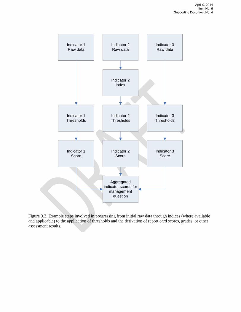
3.2.4 Thresholds and scoring Depending on the indicator, raw monitoring data may be evaluated directly by comparison to assessment thresholds, or may be converted first to an index which is then compared to assessment thresholds (Figure 3.2). Some data types, such as benthic macroinvertebrates and algae, have assessment tools that convert many separate measurements (e.g., counts of individual macroinvertebrate species) into an index of condition that can then be scored based on thresholds. Others, such as some chemical parameters, have



thresholds (including regulatory criteria) that can be applied directly to the raw data themselves. In both cases, the final result for each separate indicator will be a score or grade (as shown in Figure 3.2). Each of the four management questions includes multiple indicators. Scores for multiple indicators will be combined, or aggregated, to produce the overall score for the management question (e.g., bottom box in Figure 3.2). The workgroup considered alternative methods of weighting indicators for this final aggregation step, but concluded that all weighting approaches involve some subjective bias and that the most straightforward approach would be to treat each indicator equally (i.e., equal weights). Thus, the final management question score is based on the simple average of its component indicator scores. Because each indicator is scored on the 0 – 100 scale, the final score for the management question will also be on the 0 – 100 scale. Comparability across all indicators and management questions will be achieved by converting all indicator results to a 0 – 100 point scale. This approach has been adopted by other report card systems (e.g., CCME 2001, Council for Watershed Health 2011, USEPA 2013) and achieves the benefits of simple and consistent scaling. In addition, it allows for straightforward conversion among different scoring systems (Figure 3.3). This will be required when assessment results from other programs are integrated into the watershed report card and it is not feasible to return to and rescore the original raw data. Converting between, for example, narrative and numeric scores (as illustrated in Figure 3.3) will reduce the resolution of the scores to some extent, but has the advantage of allowing the watershed report card to integrate results from other monitoring and assessment efforts when this would otherwise not be possible. Converting numeric scoring ranges from other assessment tools to the SDRWMAP categories described in the next section may require some recalculation as described in Appendix 1.

3.3 Report card categories As described briefly above and in the following sections that detail the monitoring designs and assessment methods for each management question, all indicators will be scored on a 0 – 100 scale. While this consistent scale has the benefits of simple scaling, it does not by itself communicate conclusions about beneficial use condition. This requires translating the numeric score into narrative categories (e.g., Excellent, Good) that reflect judgments about relative condition. The workgroup therefore identified four categories of condition that are similar to those used in many other assessment and report card efforts (e.g., CCME 2001, Council for Watershed Health 2011, USEPA 2011, USFS 2011): • Excellent: Comparable with reference; absence of threat or impairment • Good: Consistently meets criteria with only rare departures from desired conditions;

beneficial uses protected with only minor threat or impairment • Fair: Usually meets criteria but beneficial uses occasionally threatened or impaired • Poor: Frequently or never meets criteria; beneficial uses frequently or usually threatened or

impaired The numeric ranges for each condition are adapted from the Canadian Water Quality Index (CCME 2001), which have also been independently derived and adopted by the Central Coast Regional Water Quality Control Board for their watershed report card (Worcester et al. in prep.). The numeric ranges were identified through an iterative process of applying index / assessment calculations using alternative thresholds and then comparing these results to the judgments and expectations of experts familiar with the monitoring data and the water bodies they were collected from. The category scoring ranges are not equally spaced along the 0 – 100 scale because, as with academic grades, only a small upper portion of the entire distribution is considered exceptional, while a much larger portion of the lower end of the distribution is considered to be performing poorly. • Excellent: 95 – 100



• Good: 80 – 94 • Fair: 65-79 • Poor: 0 – 64 In the four categories above, “Poor” results from the combination of Marginal and Poor in the CCME and Poor and Very Poor in the Central Coast Water Board’s respective report cards. In addition to these categories, which are based directly on indicator scores, the workgroup defined a separate “At Risk” descriptor that would apply to situations where enough data exist to determine they meet one or more quantitative and/or qualitative criteria suggestive of a recent or impending worsening of condition: • Significant worsening of condition as evidenced by a downward trend in assessment scores (even if

condition is not Poor) • Significant increase in stressors (e.g., recent fire or drought, upsurge in use within a specific area,

influx of invasive species, changed flow pattern) • Increased potential for intensified stress in near future (e.g., planned new development, greater access

to previously undisturbed area, likely arrival of invasive species in near future) Any assessment of At Risk will depend on the availability of trend data and the ability to integrate a variety of other types of information about condition (e.g., major events, future development plans). As a result, the application of this category may be deferred until the program is more mature.

3.4 Confidence in the assessment The aggregation and synthesis involved in scoring indicator data for the report card can obscure important data characteristics that can affect users’ confidence in the assessment results for individual indicators, aggregated indices that include multiple indicators, and the final assessment result for each management question. These characteristics include factors such as compliance with sampling and laboratory analysis protocols, the relative rigor of sampling / measurement methods, and study design elements such as the amount of data (e.g., spatial and temporal coverage). The ultimate goal of documenting such factors is to ensure users that monitoring and assessment results accurately reflect actual environmental conditions, and to provide enough information that they can intelligently interpret and apply these results. Raw monitoring data and its associated quality assurance (QA) information is typically stored in information management systems otherwise known as databases. The workgroup consulted with the QA Research Group at the Moss Landing Marine Laboratories to develop a simple scoring system (Table 3.1) to address two critical aspects of monitoring data that affect confidence in any assessments based on them: • Traditional quality control Definition

o Precision A measure of agreement among repeated measurements of the same property under identical, or substantially similar, conditions

o Accuracy A measure of the overall agreement of a measurement to a known value o Completeness A measure of the amount of valid data obtained from a measurement

system o Comparability A measure of the confidence with which one data set or method can be

compared to another o Sensitivity The capability of a method or instrument to discriminate between

measurement responses representing different levels of a variable of



interest • Study design

o Representativeness The measure of the degree to which data accurately and precisely represent a characteristic of a population, parameter variations at a sampling point, a process condition, or an environmental condition

o Design integration The extent to which the assessment questions, underlying statistical model, monitoring design, and data analysis methods are functionally linked

Concerns related to traditional quality control are typically addressed in Quality Assurance Project Plans (QAPPs) or Standard Operating Procedures (SOPs) that include data management, data assessment, and documentation, along with field and laboratory procedures. Concerns related to study design adequacy should be addressed in monitoring plans or study designs that link statistical models and sampling designs to data analyses that address motivating questions, and that control for key sources of variance and bias. The two scores in Table 3.1 (i.e., quality control and study design) would be applied to the final score or assessment result (e.g., the final, bottom box in Figure 3.1) for each management question for each time span the assessment is conducted. For example, assuming the report card assessment is conducted annually, the two confidence scores would be assigned annually to the Safe to Eat, Safe to Swim, Safe to Drink, and Aquatic Ecosystems Healthy management questions. The confidence scores in Table 3.1 would be used to judge the validity and robustness of these conclusions, to help evaluate the At Risk category, and as input to recommendations about potential management responses to assessment findings. The two confidence scores for each management question would not be combined (e.g., summed or averaged) because they provide distinctly different information about the usability or confidence of monitoring data, as illustrated in the example below: Quality

control

Study design

Average Possible judgment

Example 1 4 1 2.5 Low confidence despite high quality control because data not representative

Example 2 1 4 2.5 Moderate confidence despite low quality control because data representative

Interpretation of the quality control and study design scores, and judgments about how they would affect users’ confidence in using the data for different purposes, will necessarily depend on the goal(s) of the specific assessment. For example, screening assessments to identify the likely presence of a problem, trend assessments to determine if conditions have changed over time, and causal assessments to identify the likely source(s) of documented problems will all have distinct requirements related to data quality. The confidence scores are therefore intended as a guide to decisions about whether and how to use monitoring data in assessments, rather than as determinative standards.

3.5 Next steps Details of scoring methods and thresholds for specific indicators are included in the following chapters on each management question. As these discussions reveal, scoring methods for some indicators, particularly those being created by other parties, are pending further development and integration into the watershed report card. In addition, data for some indicators have been collected in the past by existing monitoring programs while data for new indicators (e.g., fish community structure) will be available only after the SDRWMAP has been implemented.





Table 3.1. Checklist for assessment confidence ratings for data characteristics that reflect traditional quality control (QC) concerns and a separate set of concerns related to study design. The two scores will be reported separately because they capture very different aspects of the data and would have distinct influences on decisions about the usability of monitoring data and the confidence in assessment results. Some terms such as “current data” and “adequate replication” have deliberately been left undefined because a more precise definition will depend on the specifics of the data type(s), assessment question(s), ecosystem process(es), and data analysis method(s). Confidence score

1 2 3 4 Traditional QC Informal QAPP / SOP X Formal QAPP / SOP X X Laboratory accreditation X X X Use establishedlaboratory methods X X Use established field methods X X Informal data management plan X Formal data management plan X X Data verification protocol X X Staff training program X X X Field and/or laboratory intercalibration exercises X Peer-reviewed publication(s) using data X Data entered into CEDEN or equivalent X Study design Old or limited data X Some current data X Current data X X Complete statistical model X X Reference condition defined X X X Adequate replication X Data analysis methods defined X



Safe to drink?Aquatic

ecosystems healthy?

Safe to swim? Safe to eat fish?

Comparison to thresholds,

indicator scoring & aggregation

Aquatic ecosystems score Safe to swim score Safe to eat fish

score Safe to drink score

Summary watershed assessment

Monitoring designs and raw data

Management questions

Technical program documents, links to databases

Technical reports

Beneficial use assessmentsProgram assessment reports







Figure 3.1. Basic hierarchical structure of the report card. Indicators related to each management question are scored separately and then aggregated into a score for that management question. Management question scores then provide the basis for beneficial use assessments. While the separate scores for each management question are NOT combined into a single overall score for the watershed, they can contribute to a summary of overall water condition.



Indicator 1Raw data

Indicator 1Thresholds

Indicator 1Score

Indicator 2Raw data


Indicator 2Score

Indicator 3Raw data


Indicator 3Score

Indicator 2index

Aggregated indicator scores for

management question

Figure 3.2. Example steps involved in progressing from initial raw data through indices (where available and applicable) to the application of thresholds and the derivation of report card scores, grades, or other assessment results.



100

75

50

25

0

A

B

C

D

F

Excellent

Good

Fair

Poor

100

75

50

25

0

Likely impcted

Unimpacted

Likely unimpacted

Possibly impacted

Clearly impacted

100

75

50

25

0

100

75

50

25

0

17.9

Figure 3.3. Illustration of how a numeric score that ranges from 0 – 100 can readily be converted to and from a variety of other report card scoring approaches, including narrative categories as well as letter grades. This can be accomplished by, for example, defining a numeric range for Fair (e.g., 35 – 60) and assuming that a Fair grade can be represented by the midpoint of the range, i.e., a numeric score of 47.5. While such conversions will lose resolution compared to returning to and rescoring the original raw data, they will nevertheless provide a means of readily integrating other assessment results into the watershed report card when it would be infeasible to rescore the original raw data.



4.0 Question 1: Are Our Aquatic Ecosystems Healthy? This question focuses on four beneficial uses: • Warm Freshwater Habitat (WARM) • Cold Freshwater Habitat (COLD) • Preservation of Rare and Endangered Species (RARE) • Wildlife Habitat (WILD) The question addresses concerns related to the status of streams and associated aquatic habitat in the watershed as a whole. This management question includes a number of potential assessment questions that can be grouped into the four M1 – M4 monitoring categories defined in the SDRWQCB’s Framework for Monitoring and Assessment (Busse and Posthumus 2012) and the SWAMP Assessment Framework (Bernstein 2010): • M1: Conditions monitoring and assessment

o What is the background biotic integrity in perennial streams in the watershed, as measured by indicators such as aquatic macroinvertebrates, algae, fish, and key amphibians?

• M2: Stressor identification o What are the stressors of primary concern? o What are physical / riparian habitat conditions in the watershed? o What is the distribution and abundance of aquatic invasive species in the watershed? o How much trash has accumulated in streams? o What are spatial and temporal patterns in water quality parameters, including potentially toxic

constituents, nutrients, and TDS? o Are water quality parameters above or below standardized thresholds for given sampling events? o What is the frequency of exceedances of water quality criteria?

• M3: Source identification o What are the major sources and loads of contaminant stressors? o What are the major causes of habitat modification?

• M4: Performance monitoring o Are management actions working to reduce sources of stressors? o Are conditions getting better or worse?

This information could be used by the SDRWQCB, permittees, land managers, and citizen monitoring groups to assess overall conditions in the watershed and to identify the magnitude and causes of problems in specific locations. It will also be useful in tracking progress toward meeting a range of water quality objectives. However, the SDRWMAP will begin with a focus on M1 and M2 questions related to tracking condition, status, and stressors; as such data accumulate over time they can be used in the future to focus M3 questions about sources (best addressed through special studies) and address M4 questions about trends in stressors and condition, and the performance of management actions/decisions. In overview, the monitoring design proposed to address such questions has the following main elements: • Probabilistic sampling

o Will include the entire watershed down to the upper boundary of the estuary o Treats the watershed as a single stratum, with subpopulations defined for the four subbasins

shown in Figure 1.1; subpopulations are intended to ensure a representative distribution of sampling sites across the watershed



• Targeted sampling o Sites of unique value, with an initial emphasis on combining multiple indicators at individual

sites of interest to more than one program participant o Sites along mainstem and some major tributaries to assess specific areas and issues of concern,

conducted by River Park Foundation in cooperation with other program partners o Sites to assess impacts of urban discharges, conducted by the MS4 stormwater program primarily

in the urbanized portions of the watershed • Methods and indicators

o Monitoring occurring in the spring that includes benthic macroinvertebrates, algae, basic water chemistry including nutrients, with the addition of fish communities at some sites

o Measures of physical habitat characteristics collected coincident with these indicators using the SWAMP method for measuring instream physical habitat (PHAB)

o Periodic monitoring of aquatic invasive species and trash along the mainstem and some key tributaries

o Major MS4 outfalls isnpected vidually for dry weather flows. Monitor at least five MS4 outfalls during wet weather for nutrients and conventionals, metals, and indicator bacteria. Beginning on Year 3 of the permit term, monitor highest priority MS4 outfalls with persistent flows during dry weather twice a year; during wet weather, monitor once a year. Monitoring includes field parameters (pH, temperature, specific conductivity, DO, turbidity), nutrients, conventionals, metals, and indicator bacteria. Copermittees may adjust analytical monitoring as needed if they can demonstrate that analysis for a given constituent is not necessary

Several types of data products resulting from this monitoring design are appropriate for answering Question 1 (Are our aquatic ecosystems healthy?): • From probabilistic monitoring

o Cumulative frequency distribution plots of key individual indicators or metrics and of synthesized assessment results or condition scores

o Estimates of the stream reach miles in the watershed above/below benchmarks of interest for key indicators and for synthesized assessment results

o Maps of the areal distribution of monitoring sites in the watershed above/below benchmarks of interest for key indicators and for synthesized monitoring results

o Estimates of difference in status between subpopulations o Trends over time in the estimates of watershed condition

• From targeted monitoring o Trends over time in the values of key indicators or metrics o Site-by-site comparisons in the values of key indicators or metrics o Site-by-site comparisons of indicator values and/or metrics to benchmark or reference conditions

The following subsections provide details on the design approach selected, on the several separate components of the overall approach, as well as on the recommended indicators and the sampling frequencies. A critical role for the regional program will be to coordinate the several different sampling efforts described below and to integrate their data into an overall picture of the watershed using the report card approach.

4.1 Design approach Table 4.1 illustrates the monitoring elements that will contribute to answering questions about the health of aquatic ecosystems in the watershed. Responsibility for implementation will vary depending on the program element, with the watershed program playing a central coordinating and synthesis role. The following subsections describe available technical detail for each program element. Because existing



monitoring programs have been developed for the most part independently and to answer different questions, the spatial distribution of probabilistic and targeted stations is not balanced across the entire watershed. As a result, data from both types of designs cannot simply be combined in the report card assessment without some allowance for the statistical properties of each type of monitoring data. The workgroup will address this issue as the report card is implemented and evaluated during 2014.

4.1.1 Probabilistic watershed monitoring A random, probability-based design (Table 4.1.a) is best suited to address management questions about the status of the watershed’s streams as a whole. In probability based designs, such as used by the SMC, SWAMP, U.S. EPA’s EMAP, and the Bight Program, stations are located randomly in order to provide the ability to draw statistically valid inferences about an area as a whole, rather than about just the site itself. With a probabilistic approach, conditions at site that were not sampled can be estimated. Such designs can allocate monitoring sites randomly throughout the entire region, or can subdivide the region into a number of strata or subpopulations that are relatively homogeneous. For example, the SMC’s regional (across southern California) watershed assessment program (SMC 2007) has defined three broad strata of open, agricultural, and urbanized land uses. Whatever the stratification scheme, the basic design principle is that samples are allocated randomly among strata, with the number of samples per stratum based on a consistent weighting factor (e.g., area or number of stream miles within each stratum). While probabilistic designs support conclusions about conditions across the entire watershed and about any strata defined within the watershed, they do not support conclusions about conditions at specific sites. Such sites are addressed by other program elements that include targeted sampling. The presence of multiple programs in southern California conducting condition assessments at different scales presents opportunities for coordination as well as duplication of effort and inefficiencies. Watershed programs such as the San Gabriel River Regional Monitoring Program (SGRRMP)(http://watershedhealth.org/programsandprojects/sgrrmp.aspx) and the Los Angeles River Watershed Monitoring Program (LARWMP)(http://watershedhealth.org/programsandprojects/larwmp.aspx) focus on questions at the watershed scale, the regional SMC program is focusing on the southern California region as a whole, and the State Water Board’s SWAMP looks primarily at the entire state. To prevent duplication of effort and achieve maximum sampling efficiency, the selection of randomized samples for the SDRWMAP will be based on a comprehensive sample set maintained by the Southern California Coastal Water Research Project (SCCWRP) and used by probabilistic assessment programs throughout southern California. The following subsections define: • The target population and sampling frame • Stratification and subpopulations • Sampling frequency and intensity Target population and sampling frame. The target population is the ecological resource about which information is desired and is defined by three criteria: • The San Diego River watershed down to the upper end of the estuary • Where flowing surface water exists at the time site reconnaissance is performed in the spring (an

operational definition of “perennial” used by SWAMP and the SMC pending results of ongoing work to develop a more reliable categorization of nonperennial streams and related indicators of condition)

• Channels (both natural and modified) that fit the definition of “waters of the US” along with the adjacent riparian vegetation that would typically fall under the jurisdiction of the California Department of Fish and Wildlife



More detailed definitions and descriptions of these boundary conditions follow below. Focusing strictly on freshwater simplifies the selection of sampling sites and indicators for Question 1, because it removes the need to create a separate sampling stratum and a parallel set of indicators for brackish water in the San Diego River estuary. The boundary between the San Diego River and the estuary for purposes of this program is situated at the generally accepted limit of tidal influence, which is just east of the I-5 overpass and west of the railroad right of way. However, major freshwater impoundments in the watershed were excluded from the target population, including Lake Cuyamaca, El Capitan Reservoir, San Vicente Reservoir, Lake Jennings, Santee Lakes, and Lake Murray. These are artificial water bodies and how concepts of ecosystem health would or should be applied to them requires more discussion. At present, they remain a lower priority for monitoring than natural water bodies. The target population is also defined as those portions of the watershed’s stream network where flowing water exists at the time site reconnaissance is performed in the spring. Flowing surface water was defined to include water from all sources, including natural (local) and imported water, urban runoff, and treated effluent from water reclamation plants. While this may result in the inclusion of some segments that would otherwise naturally be dry, it is difficult if not impossible to cleanly distinguish such segments and they do have the potential to support beneficial uses. Including all streams with flowing surface water (despite its source) also complies with the target population defined in the State Water Board’s developing policy for biological objectives in perennial wadeable streams. Basing the target population definition on the presence of flowing water during the spring site reconnaissance period means that 1st order streams are included in the target population. There is significant value in including 1st order streams because they make up such a large percentage of the watershed’s stream network. While these can be more difficult to access and can sometimes be dry, both the SGRRMP and LAWRMP have successfully included 1st order streams in their target populations for the past several years. Including both 1st and 2nd order streams in the target population can require additional reconnaissance effort to determine the accessibility of these smaller streams and their suitability for sampling. However, the SGRRMP and LAWRMP have found that this has not unduly increased the reconnaissance and sampling effort. They estimate that only about 10% of the streams coded as 1st or 2nd order are inaccessible. A two-step reconnaissance process would be suitable in this situation. The first step would be a desk reconnaissance based on review of maps and aerial photographs and utilizing local knowledge. The suitability of candidate streams remaining after this first step would then be further assessed with field reconnaissance. Because the amount and location of flowing water in the watershed can shift seasonally, the definition of the sampling frame (a representation of the target population used to select the sample sites and that must have the attributes needed to implement the monitoring design) should also include a time frame. Probabilistic designs based on the suite of bioassessment indicators (including algae) have standardized over the past several years on a spring sampling period for a range of reasons related to flow, the status of biological communities, and the availability of assessment tools. The proposed probabilistic watershed monitoring design thus recommends sampling in the spring, after an antecedent dry period long enough to ensure that a benthic invertebrate community is likely to have developed after any scouring from wet season storm flows. Access to some of the western portions of the watershed (i.e., San Vicente subbasin) is so difficult that they cannot be sampled within a single day. This means that it may not feasible to sample constituents with holding time constraints (particularly nutrients) at sites in these areas. Such areas might be excluded from routine sampling, sampled with a modified constituent list, or sampled periodically with a concerted effort.



Strata, subpopulations, and sampling requirements. Stratification can be used to subdivide the watershed into more homogeneous sections to better answer questions about differences between distinct portions of the watershed. However, sampling requirements in randomized designs increase linearly with the number of strata. For example, at the commonly used criterion for probabilistic assessment designs in California of 30 samples per stratum (SMC 2007), each additional stratum would require 30 additional samples for a reliable assessment. Thus, the value of increased resolution must be balanced against the associated increase in cost and effort, because each stratum requires a full complement of sampling sites. Where sampling resources are an issue, an alternative to stratification is to subsample specific areas of the watershed, i.e., subpopulations, yet still treat the watershed as a single stratum. This approach ensures representation of all subpopulations by distributing samples in desired proportions across the various sections of the watershed. The advantage of this approach is that it does not require a complete set of samples for each area of interest but instead allocates the 30 samples for the entire watershed in a way that ensures areas of interest receive adequate sampling effort. The disadvantage is that it does not allow comparison between the subpopulations of the watershed until an adequate number of samples have been accumulated. The subpopulation approach used in the SGGRMP and LARWMP (i.e., mainstem, urban tributaries, natural open space) is not feasible in the San Diego River watershed below El Capitan Dam because the majority of the mainstem is not wadeable and therefore not suitable for the standard bioassessment sampling methods. The workgroup therefore agreed on identifying the four hydrologic subbasins (Figure 1.1) as subpopulations. These reflect natural hydrologic features and substantial differences in morphology, habitat, and water quality, as well as separating urbanized from natural portions of the watershed. The four subbasins are: • Lower San Diego • San Vicente • El Capitan • Boulder Creek Sampling frequency and intensity. Sampling frequency and intensity should be selected to balance the twin goals of achieving the assessment threshold of 30 sites as quickly as possible, while also keeping in mind the longer-term relevant management timeframes. Relevant management timeframes (e.g., permit renewals, integrated 303(d)/305(b) reports) are several years long and longer-term monitoring of the results of natural processes that affect the watershed does not necessarily require frequent monitoring on an annual timescale. Thus, a complete assessment of the entire watershed on an annual basis is not necessary. Other watershed programs in southern California have adopted the following approach, which is recommended for the SDRWMAP: • Sampling the entire watershed over a five-year timeframe • Producing a new set of 30 sites on a five-year schedule appropriate to management timeframes, or an

average of six sites per year • Spreading sampling out over a number of years, which would tend to smooth or average year-to-year

variability • Keeping the level of effort to a level that realistically could be funded



4.1.2 Targeted monitoring A targeted sampling approach is best suited to answering management questions about site-specific conditions that cannot be addressed at the aggregate watershed scale, for tracking local trends, and for assessing resources and/or problems of particular concern. Depending on the question(s) being addressed, targeted monitoring designs can use a variety of statistical models to allocate sampling sites and sampling frequencies. Unlike the probabilistic component of the program, which has a consistent underlying design philosophy and statistical model, the targeted elements of the program (Table 4.1.b) have for the most part been developed independently. In addition, these programs are exclusively in the lower watershed. Programs with significant targeted monitoring elements include: • MS4 stormwater monitoring program focusing on characterizing discharges from the MS4 to

receiving waters and collecting trend data for the receiving waters • San Diego River Park Foundation River Watch program focusing on water quality • San Diego River Park Foundation RiverBlitz program for invasive plants • California Department of Fish and Wildlife fish community monitoring • California Department of Fish and Wildlife / San Diego River Park Foundation Quagga Mussel

monitoring

4.1.3 Indicators Monitoring to address Question 1 related to aquatic ecosystem health will include a number of response and stressor indicators (Figure 4.1). Some will be measured by probabilistic monitoring, some by targeted monitoring, and some by both (Table 4.1). The following paragraphs provide summary descriptions of sampling and assessment / scoring methods for each of several indicators contributing to the overall assessment of aquatic ecosystem status. Response indicators – benthic macroinvertebrates. Bioassessment, a measure of the structure of one or more components of the instream biological community, provides a direct measure, from one perspective, of the ecological status of instream communities, and it is the basis for the State Water Board’s development of biological objectives for perennial wadeable streams. Stream bioassessment programs in California have standardized around the current SWAMP bioassessment protocol which focuses on benthic macroinvertebrates, and more recently also on algae. The Southern California Index of Biotic Integrity (IBI) for benthic macroinvertebrates (Ode et al. 2005) provides a means of scoring the abundance of “bugs” in each of several taxonomic categories to derive an overall numeric score that is then categorized as illustrated in Table 4.2. These IBI scores will then be converted to the SDRWMAP’s scoring categories as described in Appendix 1. The State Water Board is expected to release a revised scoring tool, the California Stream Condition Index (CSCI), as the means of implementing biological objectives for perennial wadeable streams. While field sampling methods will remain the same, the CSCI will include different assessment algorithms as well as scoring categories and ranges. Until the CSCI is formally released, the SDRWMAP will continue using the Southern California IBI. Although the IBI is based on a 0 – 100 scale, its ranges differ from those for the watershed report card and would therefore be converted to the SDRWMAP’s scoring categories as described in Appendix 1. Efforts are underway to determine the relationship between IBI and CSCI scores, which will enable historical IBI values from part monitoring to be integrated with CSCI scores. Response indicators – algae. The amount of attached algae in a stream (i.e., percent algal cover, biomass, chlorophyll a), and its taxonomic composition, are useful indicators of nutrient overenrichment, and overall biological health in general. An recently completed Algae Index of Biotic Integrity for southern California is (Fetscher et al. 2013) is similar in structure to the benthic macroinvertebrate IBI



and includes measures of the proportion of the algal population in eight separate taxonomic categories (e.g., sedimentation tolerant, nitrogen heterotrophs) that encompass both diatoms and soft bodied algae. However, because of the challenges associated with taxonomic identification, particularly for soft bodied algae, the algae IBI will offer options that would include, for example, only diatoms or diatoms and a reduced level of taxonomic resolution for soft bodied algae. A manual of standard operating procedures for field collections was released in 2009 (Fetscher et al. 2009). The algae IBI will be scaled from 0 – 100, but its ranges are likely to differ from those for the watershed report card and would therefore be converted to the SDRWMAP’s scoring categories as described in Appendix 1. Response indicators – fish. Characteristics of the fish community can provide information about the health and functioning of the aquatic ecosystem. Indices used to evaluate the health of fish and related communities in California’s streams (e.g., Moyle and Marchetti 1999, Moyle and Randall 1998, Purdy et al. 2012) typically include metrics and scoring algorithms that measure departure from pristine conditions, particularly in terms of the distribution of native species and the prevalence of invasive species. Because the fish community in the San Diego River watershed is made up primarily of invasive or introduced (i.e., rainbow trout) species, because this situation is not likely to be reversed, and because accurate historical data are not available, the direct application of such indices would be of little value to managers. Genetics studies currently underway on upper watershed rainbow trout populations may show that one or more of these populations are descended from steelhead and are therefore native. For the present, the program’s working assumption is that all fish in the watershed are invasive or introduced, although this assumption may change as additional surveys in the upper watershed are conducted. Despite this, the current fish community in the watershed does fulfill some ecological functions and provides important beneficial uses to recreational and subsistence fishers. Thus, changes in the fish community such as increases / decreases in overall abundance or the number of species, or dramatic shifts in the age distribution, can indicate changes in the functioning of the ecosystem due to a range of natural and anthropogenic stressors, for example, the expected spread of Quagga Mussels into the lower watershed. In order to measure such changes over time, the workgroup adapted several metrics from indices used in the studies referenced above to develop an index to track changes in the fish community in the watershed over time (Table 4.3). Each metric is scored on a 1 – 5 scale and scores for the five metrics will be summed and standardized to a 0 – 100 scale (by multiplying the sum x 4) as in Moyle and Randall (1998). As in the three studies referenced above, higher scores for each metric (e.g., greater number of species) are assumed to represent better conditions. Fish index scores will be converted to the SDRWMAP’s scoring categories as described in Appendix 1. Sites will be sampled in both the upper and lower watershed. Sites in the upper watershed will be part of the probabilistic sampling design and sites in the lower watershed will be part of the targeted program component. Sites in both the upper and lower watershed will be sampled primarily with backpack electrofishing gear. The morphology and shoreline features of most of the lower river, with the possible exception of the larger RCP Block & Brick ponds between Santee and Lakeside that are currently being restored) make it impossible to access by a boat of sufficient size to carry electrofishing equipment and there are no shoreline locations suitable for using beach seines. As a result, fish surveys are not expected to sample the entire suite of species, sizes, and age classes present in the watershed and will thus provide data that can best be used to track major changes and trends in the watershed’s fish community. The fish community index includes the following five metrics: • Total number of species

o Approximately ten species present in watershed, but all habitats cannot be sampled because of accessibility constraints

o Likely to see at most six species



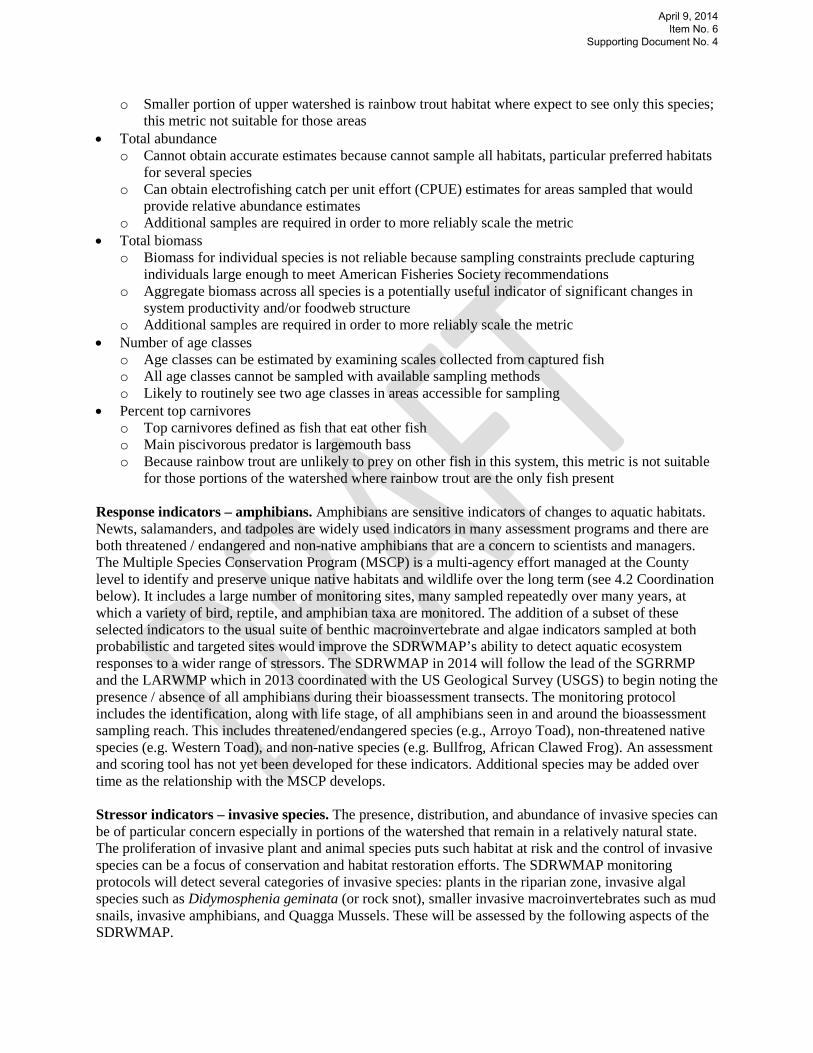
o Smaller portion of upper watershed is rainbow trout habitat where expect to see only this species; this metric not suitable for those areas

• Total abundance o Cannot obtain accurate estimates because cannot sample all habitats, particular preferred habitats

for several species o Can obtain electrofishing catch per unit effort (CPUE) estimates for areas sampled that would

provide relative abundance estimates o Additional samples are required in order to more reliably scale the metric

• Total biomass o Biomass for individual species is not reliable because sampling constraints preclude capturing

individuals large enough to meet American Fisheries Society recommendations o Aggregate biomass across all species is a potentially useful indicator of significant changes in

system productivity and/or foodweb structure o Additional samples are required in order to more reliably scale the metric

• Number of age classes o Age classes can be estimated by examining scales collected from captured fish o All age classes cannot be sampled with available sampling methods o Likely to routinely see two age classes in areas accessible for sampling

• Percent top carnivores o Top carnivores defined as fish that eat other fish o Main piscivorous predator is largemouth bass o Because rainbow trout are unlikely to prey on other fish in this system, this metric is not suitable

for those portions of the watershed where rainbow trout are the only fish present Response indicators – amphibians. Amphibians are sensitive indicators of changes to aquatic habitats. Newts, salamanders, and tadpoles are widely used indicators in many assessment programs and there are both threatened / endangered and non-native amphibians that are a concern to scientists and managers. The Multiple Species Conservation Program (MSCP) is a multi-agency effort managed at the County level to identify and preserve unique native habitats and wildlife over the long term (see 4.2 Coordination below). It includes a large number of monitoring sites, many sampled repeatedly over many years, at which a variety of bird, reptile, and amphibian taxa are monitored. The addition of a subset of these selected indicators to the usual suite of benthic macroinvertebrate and algae indicators sampled at both probabilistic and targeted sites would improve the SDRWMAP’s ability to detect aquatic ecosystem responses to a wider range of stressors. The SDRWMAP in 2014 will follow the lead of the SGRRMP and the LARWMP which in 2013 coordinated with the US Geological Survey (USGS) to begin noting the presence / absence of all amphibians during their bioassessment transects. The monitoring protocol includes the identification, along with life stage, of all amphibians seen in and around the bioassessment sampling reach. This includes threatened/endangered species (e.g., Arroyo Toad), non-threatened native species (e.g. Western Toad), and non-native species (e.g. Bullfrog, African Clawed Frog). An assessment and scoring tool has not yet been developed for these indicators. Additional species may be added over time as the relationship with the MSCP develops. Stressor indicators – invasive species. The presence, distribution, and abundance of invasive species can be of particular concern especially in portions of the watershed that remain in a relatively natural state. The proliferation of invasive plant and animal species puts such habitat at risk and the control of invasive species can be a focus of conservation and habitat restoration efforts. The SDRWMAP monitoring protocols will detect several categories of invasive species: plants in the riparian zone, invasive algal species such as Didymosphenia geminata (or rock snot), smaller invasive macroinvertebrates such as mud snails, invasive amphibians, and Quagga Mussels. These will be assessed by the following aspects of the SDRWMAP.



Invasive plants in the riparian zone are quantitatively monitored twice each year along nearly the entire length of the lower San Diego River by the San Diego River Park Foundation’s RiverBlitz program (San Diego River Park Foundation 2012). Each of ten river sections is scored on a 0 – 100 scale based on the canopy cover of eight key invasive plant species and the October scores from each year are used to assign a grade as illustrated in Table 4.4. The RiverBlitz protocol is applied to targeted segments of the lower mainstem and will be applied to probabilistic sites in conjunction with bioassessment. The RiverBlitz scores and grades will be converted to the SDRWMAP’s scoring categories as described in Appendix 1. Invasive algae will be monitored as part of the algae monitoring protocol described above. Smaller invasive macroinvertebrates will be monitored as part of the bioassessment monitoring protocol described above. Invasive amphibians will be monitored as part of the amphibian monitoring protocol described above. Quagga Mussels are a potentially damaging invasive species that are present in some reservoirs in the watershed and there is concern that they will eventually escape the reservoirs and spread through the mainstem and tributaries in the lower watershed. The San Diego River Park Foundation, in cooperation with the California Department of Fish and Wildlife, has emplaced mussel traps at three locations along the mainstem, with plans for additional sites in the future. Monitoring requirements for this indicator preclude the use of a probabilistic design because traps must be placed in sites with a specific depth range, low light, low flow, and safe access for monthly monitoring and maintenance. The three existing targeted sites are co-located with San Diego River Park Foundation River Watch monitoring sites. Metrics and scoring systems for invasive species other than invasive plants have not yet been developed. Stressor indicators – physical habitat.The SWAMP bioassessment protocol (Ode 2007) includes physical habitat metrics (PHAB) (Table 4.5) that focus primarily on the instream physical features that are useful in explaining patterns in macroinvertebrate community structure. In addition, amphibians are sensitive to specific habitat features such as specific conductance, turbidity, and stream bed / sediment characteristics. Specific conductance and turbidity will be measured as part of the conventional water quality indicator (see below) and the needed streambed / sediment metrics may be captured as part of the PHAB protocol (this has not yet been resolved). SWAMP is developing a physical habitat index based on the PHAB measurements that should be released shortly and there are habitat suitability indices for key amphibian groups (e.g., newts, salamanders). These indices have not yet been completed / identified; however, their values would be converted to the SDRWMAP’s scoring categories as described in Appendix 1. Stressor indicators – trash. Trash is currently sampled in the watershed by several programs: • MS4 copermittees at stormdrain outfalls • San Diego River Park Foundation within 30 river segments mostly in the lower watershed • San Diego Coastkeeper at one site in the lower watershed • SMC for the past two years at a combination of mostly probabilistic and some targeted sites across

the watershed The first three programs are ongoing programs and the SMC program is undergoing review and its long-term design has not yet been determined. In addition to these programs, the Bight ’13 program conducted trash monitoring for the first time as part of its regional design. The SMC and Bight ’13 efforts had comparable goals of characterizing trash across broad areas, using primarily probabilistic sampling across the entire watershed. In contrast, the other three programs have



different goals, use related but somewhat different sampling methods, and use different scoring methods to summarize and assess their results (Table 4.6). The MS4 program focuses on sites at the discharge points of MS4 outfalls with the goal of quantifying the amount of trash due to MS4 outfalls. The River Park Foundation samples trash along segments of the mainstem in the lower watershed with the goal of characterizing trash along the length of the lower mainstem and prioritizing areas for cleanup. In addition to monitoring in the lower watershed, the River Park Foundation plans to extend trash sampling into the upper watershed at probabilistic bioassessment monitoring sites. The San Diego Coastkeeper program focuses on tracking trends in trash that may be impacting coastal beaches. There are a number of possibilities for improving the sampling coordination among these programs as well as the comparability of their assessment results. These will be addressed during the 2014 implementation phase of the SDRWMAP. In the interim each trash metric will be converted to the SDRWMAP’s scoring categories as described in Appendix 1 for the initial implementation of the watershed report card. Stressor indicators – water quality. Three ongoing monitoring efforts track different aspects of water quality in the watershed: • MS4 copermittees at a variety of sites • The San Diego River Park Foundation at 15 fixed sites in the lower watershed • SMC at probabilistic sites throughout the watershed as part of the regional bioassessment program The constituents measured by each program differ and the three programs thus present different but complementary pictures of water quality: • MS4: field observations (temperature, pH, dissolved oxygen, specific conductivity, turbidity),

nutrients, conventionals (TDS, TSS, total hardness, TOC, DOC, sulfate, MBAS, total phosphorus, orthophosphate, nitrite, nitrate, TKN, ammonia), total and dissolved metals (arsenic, cadmium, chromium, copper, iron, lead, mercury, nickel, selenium, thallium, zinc), pesticides (organophosphates and pyrethroids), indicator bacteria (total coliform, fecal coliform, Enterococcus), bioassessment, toxicity, and hydromodification.

• San Diego River Park Foundation: temperature, pH, dissolved oxygen, specific conductivity, nitrate, phosphate

• SMC: conventionals (temperature, pH, conductivity, dissolved oxygen, alkalinity, hardness), nutrients (ammonia, nitrite, nitrate), pyrethroid pesticides

The San Diego River Park Foundation has developed a scoring index that integrates its water quality parameters, but scoring metrics for the MS4 and SMC parameters have not yet been developed. One goal of the implementation effort in 2014 will be to develop a means of integrating the various water quality monitoring results into a more comprehensive assessment at the watershed scale. One approach might be the method based on frequency and magnitude of exceedances of threshold values, as described in Section 5.3 below.

4.2 Coordination As Table 4.1 and the preceding discussion make clear, completion of an assessment report card for the entire watershed will require coordinating the respective monitoring and assessment efforts of multiple programs and then integrating their data into an overall assessment framework. Thus, unlike other watershed programs in the Los Angeles, San Gabriel, and Santa Clara Rivers watersheds that are implemented primarily by a single entity (albeit with the support of stakeholder workgroups), the SDRWMAP will necessarily include a much greater degree of outreach, coordination, and data



integration. For example, the State Water Board’s Biological Objectives for Perennial Streams and Nutrient Numeric Endpoints (NNE) policies will define expectations or endpoints that will fill gaps in the watershed report card related to assessment criteria. These could be combined or integrated with the indicator scoring criteria in the Forest Service’s Watershed Condition Framework to achieve a set of comparable assessment criteria watershed wide. The San Diego are MSCP is another likely candidate for further coordination. The MSCP is a subregional plan under the Natural Communities Conservation Planning Act, which is implemented through local subarea plans. The California Department of Fish and Wildlife administers the Natural Community Conservation Planning (NCCP) program, a California regional habitat conservation planning program. Both the City and County of San Diego participate in the NCCP program by implementing their respective MSCP Subarea Plan (SAP). In addition to sharing indicators and monitoring methods as described above, there is potential for collaboration on integrated sampling designs, assessment methods, and report card approaches. Table 4.1 also identifies several management questions related to site-specific concerns and/or stressor identification that could be answered with information produced by site-specific special studies, results of the stressor response modeling being conducted by the Biological Objectives policy development team, or the results of the stressor identification case study that was conducted for the San Diego River watershed in 2012 and 2013.



Table 4.1.a.Design overview for the probabilistic component of the regional monitoring program for aquatic ecosystem health. Design element

Description Details

Design approach Probabilistic All channels with flowing water, including 1st and 2nd order streams Excludes impoundments and lakes Watershed treated as one stratum with three subpopulations (mainstem, urban tributaries,

natural open space)

Number of sites 6 per year All sites selected randomly, representative distribution across three subpopulations

Sampling frequency Yearly in spring

Standard SWAMP index period

Response indicators

Bioassessment indicators Stream benthic macroinvertebrates Algae

SWAMP bioassessment macroinvertebrate sampling protocol SWAMP benthic algae sampling protocol

Fish Resident fish community

Community measures at bioassessment sites; methods dependent on habitat conditions and site accessibility

Amphibians

All amphibians encountered Presence / absence and life stage of all native amphibians encountered during bioassessment sampling

Stressor indicators

Invasive species indicators 8 key invasive riparian plants Algae Small macroinvertebrates Amphibians

SD River Park Foundation RiverBlitz sampling protocol SWAMPbenthic algae sampling protocol SWAMP bioassessment macroinvertebrate sampling protocol Presence / absence and life stage of all non-native amphibians encountered

Habitat indicators Physical habitat Aquatic chemistry

SWAMP PHAB sampling protocol Amphibian habitat metrics Trash using SD River Park Foundation sampling protocol Conventionals (hardness, pH, dissolved oxygen, TDS) Nutrients



Table 4.1.b. Design overview for the targeted component of the regional monitoring program for aquatic ecosystem health. Design element

Description Details

Design approach Targeted Sites that address management questions tied to specific locations Number of sites, sampling frequency, and indicators vary depending on program and indicator

Response indicators

Bioassessment indicators Stream macroinvertebrates Algae

1 long-term MS4 site using SWAMP bioassessment macroinvertebrate sampling protocol 1 long-term MS4 site using SWAMP benthic algae sampling protocol

Fish Resident fish community Five sites at specific habitat types in lower watershed, sampled with hoop nets and hook and line

Stressor indicators Invasive species indicators 8 invasive riparian plants

Quagga mussel 10 zones along lower river, SD River Park Foundation RiverBlitz protocol, twice yearly 3 sites in high risk areas in lower river, colocated with SD River Park Foundation River Watch

sites

Stressors Aquatic chemistry Physical habitat

5 MS4 sites for conventional chemistry and key pollutants 10 zones along lower river, SD River Park Foundation River Watch sampling protocol SWAMP PHAB sampling protocol at bioassessment sites Amphibian habitat metrics at bioassessment sites Trash using SD River Park Foundation sampling protocol Trash using MS4 sampling protocol



Table 4.2. Southern California Index of Biotic Integrity (IBI) scores for macroinvertebrate bioassessment. The IBI scores will be adjusted to the SDRWMAP’s report scale as described in Appendix 1.

Southern California IBI score

IBI condition

80 - 100 Very Good 60 – 79 Good 40 – 59 Fair 20 – 39 Poor 0 – 19 Very Poor



Table 4.3. Fish community metrics and scoring ranges, adapted from Moyle and Marchetti (1999), Moyle and Randall (1998), and Purdy et al. (2012). Scores for each metric will be added and the sum multiplied x 4 to normalize the scores to a 0 – 100 scale and then be adjusted to the SDRWMAP’s report scale as described in Appendix 1. Metric Scoring Notes

Total # species 1: <3 3: 3 – 5 5: >5

Not applicable to rainbow trout habitat in upper watershed tributaries where rainbow trout is the only species present

Relative abundance 1 – 5 scale

Scoring ranges will be finalized once data from additional surveys are available

Total biomass 1 – 5 scale

Scoring ranges will be finalized once data from additional surveys are available

# age classes 1: 0 – 1 3: 2 5: 3+

% top carnivores 1: <5% 3: 5 – 10% 5: >10%

Not applicable to rainbow trout habitat in upper watershed tributaries where rainbow trout is the only species present



Table 4.4. Scoring ranges and corresponding assessment grades for the San Diego River Park Foundation’s RiverBlitz invasive riparian plant monitoring program. Scores will be adjusted to the SDRWMAP’s report scale as described in Appendix 1.

% Cover of invasive non-native

Score

Assessment grade

0 – 1 90 – 100 A – Excellent 1.1 – 2 80 – 89.9 B – Good 2.1 – 3 70 – 79.9 C – Fair 3.1 – 4 60 – 69.9 D – Marginal >4.1 0 – 59.9 F – Poor



Table 4.5. Physical habitat parameters sampled in the SWAMP 07 PHAB approach. Scoring and conversion to the SDRWMAP report card scoring categories will be deferred until SWAMP releases the PHAB index. Aspect of system

SWAMP 07 physical habitat quality

Hydrology Channel flow status: amount of discharge; bank full width, bank full depth, wetted width

Hydrology/physical structure Velocity/depth regime: % of pools, riffles, runs, glides, cascades

and falls

Physical structure/substrate Sediment composition: pebble counts along eleven transects converted to percent composition

Embeddedness: % embeddedness of 21 cobbles along entire reach

Physical structure Channel alteration: presence of channelization or bank hardening

Bank stability: presence of erosion along banks

Physical structure/habitat Epifaunal substrate/available cover: presence of submerged habitat such as snags, cobble beds, etc.

Frequency of riffles, frequency and distance between riffles

Habitat Vegetation protection: extent and diversity of habitat along the streambanks including canopy, mid canopy and ground cover

Riparian vegetative zone width: width of riparian zone and presence of human activities

Human activities: roads, structures, trash, mining, etc.



Table 4.6. Comparison of trash scoring metrics and ranges for the San Diego River Park Foundation (SDRPF) and MS4 trash sampling programs. Pending possible improved coordination among programs, scores for each program will be adjusted to the SDRWMAP’s report card scale as described in Appendix 1.

Bags / acre

Numeric score

Color

SDRPF grade

MS4 grade

<1 A (90-100) Excellent Optimal 1.0-1.9 B (80-89.9) Good Suboptimal 2.0-2.9 C (70-79.9) Fair Marginal 3.0-3.9 D (60-69.9) Marginal Poor

>4 F (0-59.9) Poor



Figure 4.1. Conceptual structure of the watershed report card for aquatic ecosystem health assessment. Indicators are scored individually (i.e., 1st level indices or scores) and then grouped into four categories. The report card score for each of the four categories is calculated as the average (i.e., 2nd level indices or scores) of the individual indicator scores in each category. The four category scores are not averaged further (as indicated by the horizontal dashed line), but may be synthesized as part of an overall narrative assessment of aquatic ecosystem status.

Bugs Algae Fish Invasive plants

Invasive mussels,

othersPHAB Flow

Amphibian habitat parms

Conduc-tivity

Temp, DO

1st level indices or scores

Biology assessment score

Habitat-related stressors

assessment score

Water quality stressors

assessment score

2nd level indices or scores

Biological stressors

assessment score

Narrative Aquatic Ecosystem Health Assessment

Nutrients

Raw data / indicators Raw data

Thresholds

Assessment results / grades

Thresholds / index algorithms

TurbidityTadpoles, etc. Trash

Average of scores

Synthesis



5.0 Question 2: Is It Safe to Swim in Our Waters?

5.1 Monitoring questions and data products This question focuses on the portion of the beneficial use Water Contact Recreation (REC1) that includes full-immersion activities, termed “swimming” here. The workgroup determined that, while REC2 activities (e.g., fishing from float tubes) occur in the watershed, limited monitoring resources would best be allocated to the higher risk activity (i.e., full immersion). Question 2 reflects concerns about the risk posed by pathogen contamination to recreational users of the San Diego River, its tributaries, and swimming lakes. There are a number of lakes in the watershed, none of which allow swimming, although there are several locations in streams that are popular swimming sites. While most of these are not officially designated and managed as swimming sites, they are in locations with public access and body contact recreation is allowed. There are three key assessment questions that address these concerns (see also Table 2.1): • M1: Condition monitoring and assessment

o Are bacterial indicator levels at locations in the watershed with the highest observed recreational use above water quality objectives?

• M3: Source identification o What are potential sources of bacteria that could be affecting swimming sites?

• M4: Performance monitoring o Are conditions getting better or worse?

Questions related to stressor identification (M2) are not relevant here because the indicators themselves are the stressors. This information could be used by the SDRWQCB and by the health services departments for the County of San Diego and the cities in the watershed to help manage health risk. Monitoring data could also be used by the SDRWQCB and program participants to develop management actions in the event contamination at swimming sites is found. In overview, the monitoring design to address such questions includes three main elements that involve targeted monitoring: • Monitoring five times per month during the swimming season at sites with the highest observed

swimming use • Use of total and fecal coliforms, Enterococcus, and E. coli as the indicators at freshwater swimming

sites • Targeted special studies to identify potential sources of contamination in the event contamination is

documented at swimming sites Several types of data products resulting from this monitoring design are appropriate for answering Question 2 (Is it safe to swim in our waters?): • Measures of bacterial indicators at individual swimming sites • Comparisons of bacterial indicator values with relevant standards or objectives (e.g., data tables or

charts that highlight exceedances)



• Trends over time in bacteria levels and in exceedance index values at individual swimming sites and aggregated over the watershed

• Information on sources of contamination at swimming sites The following subsections provide details on the design approach, as well as on indicators, sampling sites, sampling frequencies, and data analysis and assessment approaches.

5.1 Design approach While there are Basin Plan standards for inland waters designated for REC1 use, these have not been applied to monitoring targeted at popular inland swimming sites because attention has focused on coastal beaches where swimming use, and thus potential human exposure and risk, is much greater. Monitoring of bacterial indicators was conducted under the most recent NPDES permit for urban runoff (i.e., stormwater) at a small number of receiving water stations associated with stormwater discharges and at one mass loading station. However, this monitoring does not address the questions associated with potential human health impacts at inland swimming sties for two primary reasons. First, some of these stations are in channels where swimming may be prohibited and none of this monitoring is targeted specifically at swimming locations. Second, much of the swimming activity in the watershed takes place outside of the urban areas where the urban runoff monitoring program is focused; as a result there is no information about potential levels of bacterial contamination at the most popular swimming sites. The recommended monitoring approach (Table 5.1) to address the management questions includes three separate components, including: • An initial use assessment survey to finalize the list of swimming sites to be monitored over the longer

term • Monitoring in subsequent years of bacterial indicators at high priority swimming sites • Targeted source identification studies in the event contamination is found There is an important distinction between swimming activities in the watershed’s lakes (all of which are reservoirs) and streams. Swimming (i.e., full body immersion) is prohibited in all the watershed’s reservoirs because of concerns about potential contamination of drinking water supplies. There are no designated swimming beaches and some reservoirs (e.g., El Capitan) actively patrol to enforce the swimming ban. However, El Capitan does allow water skiing and wake boarding (as will San Vicente when it reopens in approximately 2 – 4 years), as well as the use of float tubes, kayaks, and canoes. These activities can result in brief, incidental full immersion and these two lakes are therefore included on the list of swimming sites. As part of the permit for this limited body contact, the City of San Diego has for the past 15 years been required to monitor coliform levels in the reservoirs and submit results to the County Department of Environmental Health. This monitoring will be supplemented by the addition of Escherichia coli (abbreviated E. coli) and Enterococcus to include the full suite of indicators for this management question. Full body immersion swimming does occur regularly in several stream locations in the watershed, although these are not currently managed as designated swimming areas. The workgroup identified the following list of candidate monitoring locations in streams in the watershed: • Three Sisters Falls • Cedar Creek Falls • Boulder Creek – Gold Mine Pond • Ritchie



• Devil’s Punch Bowl • Mission Valley Preserve Most of these candidate monitoring sites are in the upper watershed because there is little swimming in the lower San Diego River below the reservoirs, although this portion of the river is designated as the REC-1 beneficial use. While swimming sites in the river and tributaries are generally unmanaged, the USFS is implementing a daily permit system to manage the amount of use at Cedar Creek Falls. Users would have to obtain a day use permit and the number of these would be capped to minimize damage to the access trail, the swimming area, and surrounding habitat. Because the intensity of recreational activity differs among sites and may be limited at some sites to wading, monitoring during the program’s first year should focus on a field survey of the relative amount of swimming at each site. In addition, monitoring may be a lower priority at sites where flow is highly intermittent and swimming use therefore lower. This initial use survey should include one weekday and one weekend day at each site during the May 1 through September 30 swimming season. This survey will provide data that responds to the SDRWQCB’s 2011 Basin Plan Staff Report that suggested defining tiers of the REC-1 designation based on frequency of use. This initial use survey should also be coordinated with any recreational use assessments conducted as part of efforts to develop information relevant to the bacteria TMDL. This coordination should focus on preventing any duplication of effort and on ensuring that survey designs are comparable and allow data from throughout the watershed to be combined. Depending on the survey results, the list of sites could be revised as needed to ensure monitoring is focused on the highest priority sites. Depending on the site, sources of indicator bacteria and pathogen contamination include human contact recreation, wildlife, leaking septic systems, urban runoff, and campgrounds. While source identification could be an important aspect of the SDRWMAP in the future, specific source identification efforts are not included in the initial implementation of the regional watershed program. Bacterial source identification studies can be intensive and are best implemented once condition (i.e., presence, extent, magnitude of contamination) has been established. Based on experience monitoring inland swimming sites in the San Gabriel and Los Angeles Rivers watersheds, it may require two or three years of monitoring to adequately characterize patterns of bacterial contamination. For planning purposes, it is assumed that monitoring at the final set of swimming sites will be conducted five times per month (to produce sufficient data to calculate the monthly geometric mean of indicator values) during the swimming season, since there is little if any swimming during the winter. Based on the protocol used in the SGRRMP, LARWMP, and SCRWMP, one location per site will be sampled, immediately downstream of the swimming area. This location maximizes the contamination signal and ease of sampling. Sampling locations and times may be adjusted occasionally to concentrate sampling on periods of heavier use (e.g., weekends, holidays) and the days immediately following these. The SGRRMP and LARWMP have seen some evidence that increased use is associated with higher indicator values and the availability of additional data from the San Diego River watershed could improve the ability to assess whether this pattern actually exists.

5.2 Indicators The present state standard for freshwater is based on E. coli. The USEPA has strongly advocated in its recent guidance (USEPA 2012) that freshwater standards be revised to include Enterococcus, based on its better relationship to actual health risk. However, making this change will require several years at least. In addition, the Basin Plan objectives for the San Diego Region include fecal coliforms and the bacteria TMDL in the San Diego Region is based on this indicator. There are substantial reasons for moving away from the fecal coliforms indicator in the long run. The larger category of fecal coliforms can include



coliforms from vegetation sources and soils which are not associated with pathogens that pose health risk to humans. Both E. coli and Enterococcus more closely reflect human health risk. In addition, the laboratory method for analyzing fecal coliforms is susceptible to bias from high turbidity and is more time consuming than that for other indicators. Despite USEPA’s recommendation that states move away from fecal coliforms as a freshwater standard, the monitoring at swimming sites is recommended to focus on all three indicators for the present. E. coli is the current primary public health criterion and is also the indicator used in other watershed monitoring programs in southern California (SGRRMP, LARWMP, SCRWMP), fecal coliforms are in the current Basin Plan, and Enterococcus provides better information for managers and is likely to be the basis for future standards and regulations. As the standards evolve, the SDRWMAP may reduce the number of indicators by dropping fecal coliforms and perhaps E. coli as well.

5.3 Thresholds and scoring Thresholds for the three indicators (Table 5.3) are drawn from Basin Plan objectives for fecal coliforms and current USEPA guidance for E. coli and Enterococcus. USEPA proposes two sets of thresholds, one calibrated to an illness rate of 32 / 1,000 and a second, less restrictive one, to an illness rate of 36 / 1,000. The workgroup selected the less restrictive thresholds because the numbers of swimmers utilizing these sites is relatively low compared to use at beaches, full immersion swimming is not permitted in reservoirs, and stream swimming sites are not formally designated and managed as such. Data from the three indicators will be aggregated into an index using the Canadian Water Quality Index (CCME 2001), which is a method for integrating the proportion of failed variables, the proportion of failed tests, and the amplitude, or magnitude, of exceedances across multiple indicators. Together, these summarize key aspects of the pattern of exceedances. This approach is appropriate here because each of the three indicators has clear thresholds for impairment, and evaluation of the degree of impairment focuses primarily on the number and frequency of exceedances. Three factors make up the Canadian Water Quality Index (CCME 2001), which reflect different aspects of indicator behavior relative to regulatory thresholds. The equations below are structured to produce a final index score on the 0 – 100 scale, with the equation for excursion in Factor 3 structured for indicators that must not exceed the objective value. Unlike Factors 1 and 2, Factor 3 requires three steps for its calculation. In this index, “variable” is an indicator such as E. coli or Enterococcus, “test” is every individual comparison of a data value to a standard or objective (e.g., Enterococcus geometric mean, Enterococcus single sample maximum)

Factor 1: Scope, or percent of tested variables that did not meet objectives

Factor 2: Frequency, or percent of individual tests that do not meet objectives



Factor 3: Amplitude, or the cumulative amount by which failed test values do not meet their objectives, calculated in three steps

where nse = normalized sum of excursions

In the definition of Factor 1 above, there will be six “tested variables,” including the geometric mean for each of the three bacterial indicators and the maximum exceedance rate for the three indicators. Thus, in a given test period, the percent of tested variables not meeting objectives could range from 16.67% (i.e., 1/6) to 100% (i.e., 6/6). In the definition of Factor 2, the “percent of individual tests” refers to the fraction of the total number of comparisons to objectives that fail. Thus, for a single site in the summer swimming season, there would be: 5 samples / month x 5 months x 6 tests per sampling event = 150 individual tests. If, for example, 25 of these tests did not meet their respective objective, then the percent failure rate would be 25/150 = 1/6 = 16.67%. In the definition of Factor 3, the “cumulative amount” by which tests fail is simply the overall sum of the magnitude of each exceedance of an objective. These exceedances are normalized by the calculations shown above. The index itself is calculated as the quadratic mean (or root mean square) of the three factors, which gives greater weight to larger values, thus emphasizing excursions.

The final water quality index for bacteria is scaled 0 – 100 and threshold ranges for the report card categories are as defined in Section 3 above: • Excellent: 95 – 100 • Good: 80 – 94 • Fair: 65-79 • Poor: 0 – 64

5.4 Coordination with other efforts It would be useful to compare the results of monitoring at swimming sites with those from similar programs in the Los Angeles River, San Gabriel River, and Santa Clara River watersheds. This could provide insight into contamination patterns and the larger number of samples in a combined dataset would improve the statistical power of any analyses. Results from this program component could potentially be useful to the ongoing bacteria TMDL mplementation program in the San Diego Region. However, the TMDL compliance point is at the lower



end of the watershed, below all of the potential swimming sites listed in Table 5.2, which means that data from swimming sites will not be suitable for assessing TMDL compliance. Results of the initial use survey of inland swimming sites could be useful in updating the Regional Water Board’s understanding of the intensity of the REC1 swimming beneficial use in the watershed. While the bacteria TMDL allocates 100% of the bacteria load to the MS4, any future targeted source identification studies at inland swimming sites could help update understanding of sources of bacterial contamination. There are likely to be only limited opportunities for coordination of this program component with other components of the watershed monitoring program. This is primarily because monitoring sites selected based on their swimming use will most likely not correspond to sites chosen to address other water quality and/or habitat concerns. In addition, bacteria monitoring for human health typically occurs on a schedule that is much more frequent than the sampling envisioned for much of the rest of the regional monitoring program. However, monitoring at stream sites could be conducted in cooperation with volunteer organizations and/or the Forest Service, for those sites within the National Forest boundary.



Table 5.1. Design overview for the recreational swimming component of the regional monitoring program. Design element

Description Details

Design approach

Preliminary use survey to finalize swimming sites

Swimming sites Sentinel sites Mass loading sites

Document relative degree of swimming; conduct in coordination with TMDL program

Monitor during swimming season Random or fixed sites to assess background conditions

and track trends in conditions; establish in coordination with TMDL program

Fixed sites to measure loadings and trends in these; establish in coordination with TMDL program

Number of sites Use survey: 6 stream Swimming: 8 (2 lakes, 6 stream)

Likely swimming locations Most frequently used swimming locations

Sampling frequency Use survey: twice weekly Swimming: 5 / month

One weekday and one weekend day, from May 1 through September 30

May 1 through September 30

Indicators Swimming Fecal coliforms, E. coli, Enterococcus



Table 5.2.Locations in the San Diego River watershed where swimming is known to occur. Swimming location

Detail

El Capitan Reservoir

Reservoir, swimming prohibited, incidental body contact and immersion

San Vicente Reservoir Reservoir, swimming prohibited, incidental body contact and immersion, not filled for 3 – 5 more years

Three Sisters Falls

National Forest, difficult access, low use

Cedar Creek Falls National Forest with trail access, moderate to heavy use with more than 100 people in the water at times

Boulder Creek – Gold Mine Pond

National Forest with access across a small piece of private land

Ritchie

Devil’s Punch Bowl

National Forest, low use

Mission Valley Preserve

Combination of riffles and deeper pool; regular use by waders, homeless population, and bicyclists who use ramp to jump into river



Table 5.3. Exceedance thresholds for the three indicators used to assess human health risk due to swimming in freshwater streams, creeks, and the mainstem in the San Diego River watershed. Indicator

Threshold Detail

Basin Plan Fecal coliforms 200 cfu / 100 ml

10% > 400/100 ml

Log or geometric mean of minimum 5 samples in 30 day period

Maximum exceedance rate for 30 day period

USEPA 2012 criteria #1 Illness rate 36 / 1,000 E. coli 126 cfu / 100 ml

10% > 410 cfu / 100 ml



Enterococcus 35 cfu / 100 ml 10% > 130 cfu / 100 ml





Figure 5.1. Candidate monitoring locations to address potential human health risks from swimming in the San Diego River watershed. Full body immersion is not permitted in El Capitan and San Vicente Reservoirs, but bacterial indicator monitoring will help characterize risk from incidental contact due to kayaking, water skiiing, and other similar recreational activities.



Fecal coliforms data E.coli data Enterococcus data

Thresholds

Factor 1, 2, 3 scores

Safe to Swim assessment score

Aggregation algorithm

Figure 5.2. Structure of indicators and scoring for the Safe to Swim management question. Thresholds are defined by regulatory criteria and/or guidance and the scoring and aggregation algorithms are based on the Canadian Water Quality Index.



6.0 Question 3: Is It Safe to Eat Fish and Shellfish From Our Waters?

6.1 Monitoring questions and data products This question focuses on the beneficial use Commercial and Sport Fishing (COMM) and reflects concerns related to the safety of eating locally caught fish. There are several assessment questions that address such concerns: • M1: Condition monitoring and assessment

o At the most frequently fished sites, what are the concentrations of chemical contaminants in the tissues of commonly consumed target species?

o How do these tissue levels of contaminants compare to critical thresholds of potential human health risk?

o At the most frequently fished sites, what are the trends in tissue concentrations of chemical contaminants in commonly consumed target species?

This information could be used by the SDRWQCB and other management agencies at the regional and statewide level to help manage health risk and address sources of tissue contamination. Other than the statewide survey of lakes by SWAMP’s Bioaccumulation Oversight Group, which sampled El Capitan and San Vicente Reservoirs and Lake Jennings, and some earlier historic data from the 1980s and 1990s, there are currently no fish tissue data available for the watershed. Monitoring at a larger number of lakes and at stream fishing sites would complement the SWAMP survey and provide local managers with a more complete dataset for responding to concerns about the safety of consuming locally caught fish. The SWAMP lakes survey found that tissue levels in Region 9 were in general lower than elsewhere in the state and that only mercury in largemouth bass in El Capitan and San Vicente Reservoirs had elevated levels that would restrict human consumption (one meal per week). The SWAMP stream survey did not sample sites in the San Diego region. In overview, the monitoring design (Table 6.1) recommended to address such questions has several elements: • An initial small screening survey to assess contaminant levels in fish tissue at a site on the San Diego

River at Old Mission Dam was conducted to begin adding to historical trend data from this site and to identify logistical issues related to the larger sampling effort to begin this year (2014)

• A consumption survey to identify the most commonly consumed fish species and to confirm the preliminary selection of fishing sites

• Focus on the six lakes and nine stream sites where most fishing occurs • Sample three sites each year in summer and rotate sampling among the sites on a five year schedule • Focus on fish species most commonly caught and consumed at each site • Focus on the chemicals (mercury, DDTs, PCBs, selenium) ingested with California’s sport fish that

contribute the greatest to human health risk, and known emerging chemicals of concern for bioaccumulation (e.g., PBDEs)

Several types of data products are appropriate for answering Question 3 (Is it safe to eat fish and shellfish from our waters?):



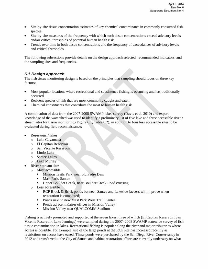
• Site-by-site tissue concentration estimates of key chemical contaminants in commonly consumed fish species

• Site-by-site measures of the frequency with which such tissue concentrations exceed advisory levels and/or critical thresholds of potential human health risk

• Trends over time in both tissue concentrations and the frequency of exceedances of advisory levels and critical thresholds

The following subsections provide details on the design approach selected, recommended indicators, and the sampling sites and frequencies.

6.1 Design approach The fish tissue monitoring design is based on the principles that sampling should focus on three key factors: • Most popular locations where recreational and subsistence fishing is occurring and has traditionally

occurred • Resident species of fish that are most commonly caught and eaten • Chemical constituents that contribute the most to human health risk A combination of data from the 2007-2008 SWAMP lakes survey (Davis et al. 2010) and expert knowledge of the watershed was used to identify a preliminary list of five lake and three accessible river / stream sites for tissue monitoring (Figure 6.1, Table 8.2), in addition to four less accessible sites to be evaluated during field reconnaissance: • Reservoirs / lakes

o Lake Cuyamaca o El Capitan Reservoir o San Vicente Reservoir o Lindo Lake o Santee Lakes o Lake Murray

• River / stream sites o Most accessible Mission Trails Park, near old Padre Dam Mast Park, Santee Upper Boulder Creek, near Boulder Creek Road crossing

o Less accessible RCP Block & Brick ponds between Santee and Lakeside (access will improve when

restoration is completed) Ponds next to new Mast Park West Trail, Santee Ponds adjacent Kaiser offices in Mission Valley Mission Valley near QUALCOMM Stadium

Fishing is actively promoted and supported at the seven lakes, three of which (El Capitan Reservoir, San Vicente Reservoir, Lake Jennings) were sampled during the 2007- 2008 SWAMP statewide survey of fish tissue contamination in lakes. Recreational fishing is popular along the river and major tributaries where access is possible. For example, use of the large ponds at the RCP site has increased recently as restrictions on access have eased. These ponds were purchased by the San Diego River Conservancy in 2012 and transferred to the City of Santee and habitat restoration efforts are currently underway on what



is now termed the Walker Preserve. While the current focus is not habitat restoration, future plans include improved fishing access to the ponds. Many other potential fishing sites are used little if at all for recreational fishing because of legal restrictions on access or because they are too overgrown to reach. In addition to recreational fishing, subsistence fishing occurs at several locations along the lower mainstem of the river, mostly conducted by a small but persistent population of homeless individuals. This information will be confirmed and/or updated by the consumption survey (see Section 6.2.1 below) and additional field reconnaissance before the final set of sampling sites is identified. While recreational fishing occurs at Lake Jennings, it was not included on the list of sampling sites because the SWAMP survey documented very low levels of contaminants in tissue samples from this site. In addition, Lake Jennings, which is a forebay for the Helix Water District’s filtration plant, does not convey or release water through the watershed and is filled with imported water from outside the watershed. Thus, any contaminants found in fish tissue from Lake Jennings would not have originated within the watershed (throughput of imported water is so large that local atmospheric deposition is not likely to be a major source). Tissue sampling is recommended to occur in the summer to correspond with a number of other regional monitoring programs in southern California (e.g., SWAMP, Bight Program, SMC, SGRRMP, LARWMP) that use the spring or summer as their index sampling period. Fishing has been observed to be most common along the river during warm weather, while fishing occurs year round at the lakes. Despite some seasonal variation in fishing effort, sampling at a consistent time of year will help to minimize potential sources of temporal variability by avoiding seasonal fluctuations in several factors: • Fish populations and assemblages • Tissue contaminant concentrations associated with spawning cycles • Angling effort • Angling populations (e.g., children vs. adults) • Tissue types (e.g., more roe in whole fish samples during some seasons) • Stocking schedules, especially for channel catfish • Runoff water inflow associated with variable storm magnitudes Attempting to control for all these potential sources of variability would require a more complex monitoring design with substantially higher costs resulting from additional sampling and tissue analysis. Based on several years of experience with tissue sampling in other regional and statewide programs, tissue sampling need not occur annually at every site because tissue levels for the targeted contaminants change only slowly. For example, DDT and PCB were banned many years ago and there are not readily controllable point sources for either of these contaminants or for mercury. Background levels are thus likely to change only slowly. Sampling once every five years will be adequate to track trends, although this planned frequency may be changed in the future depending on the specific information needed for decision making. For example, if tissue levels of target chemicals are far above accepted screening values or action levels, and 303(d) delisting and/or removal of consumption advisories is unlikely, then infrequent sampling, perhaps as little as once every ten years, may be appropriate for long-term trend tracking. Conversely, if tissue levels or target chemicals are far below screening values or action levels, and there is no information to suggest they will rise rapidly (e.g., as is the case for legacy pollutants), then infrequent sampling may also be called for. However, if tissue levels are near critical values at which key management decisions would be made, then annual (or more frequent) sampling might be needed to guide such decisions. This general framework, adapted from Bernstein et al. (1999), is summarized below.



Tissue level relative to decision threshold

Sampling frequency

Far above Infrequent, every 10 years Near Frequent, e.g., annual Far below Infrequent, every 10 years Thus, the initial sampling schedule of three sites per year with all sites sampled on a five-year rotating schedule could be modified based on monitoring results and factors that could influence levels of management concern (e.g., tissue level relative to OEHHA thresholds, rate of increase/decrease in tissue levels, size and makeup of exposed population).

6.2 Indicators Indicators fall into two major categories, the species of fish to be sampled and the chemical constituents to measure in their tissue.

6.2.1 Target species The information in Table 6.2, which summarizes readily available knowledge about the fish most commonly caught at each of the proposed sites, provides a starting point for identifying target species, as does the SWAMP list of target species for lakes (Table 6.3) and catch data collected by lake managers. However, this information is either anecdotal (Table 6.2), generic (Table 6.3), or restricted only to catch and does not account for site-specific differences due to ecological conditions, the history of introduced species, and current and past stocking practices. In addition, the SWAMP list does not incorporate information on angler preferences and none of the available data focus on consumption practices. For this reason, the SDRWMAP workgroup agreed to conduct an angler consumption survey at river and lake fishing sites before finalizing the list of sampling sites and target species. Four consumption studies, one conducted in the San Diego River watershed by the River Park Foundation and three others (Allen et al. 1994, 2008, Monohan et al. 2011) conducted elsewhere in the state, provided a representative cross section of survey methods to choose from. The workgroup drew from these reports to design a consumption study for lake and river fishing locations in the San Diego River watershed. The study used a combination of access point surveys (e.g., at boat launch ramps, trailheads leading to the river) and roving surveys (e.g., float tubes along the river) to gather information on fishing practices, most frequently caught species, and consumption patterns, including methods of preparation (e.g., skin on / off fillets, whole body). It is recommended that rainbow trout not be sampled in lakes. This is the approach taken by other watershed monitoring programs in southern California because rainbow trout are generally caught very quickly after their release. As a result, their tissue contaminant levels most likely reflect their feedstock rather than conditions in the lakes. In contrast, channel catfish, another widely stocked species, is released at smaller sizes and survives for much longer. Similarly, rainbow trout released into the upper watershed can survive for more than a year and thus have the potential to accumulate contaminants from the watershed; they are therefore included on the target species list for stream sampling

6.2.2 Tissue analyses Muscle tissue from fish collected at each location would be combined into a single composite sample for each species for analysis. Sampling will follow the SWAMP guidelines (SWAMP 2007, 2011), which specify a minimum number of five fish per composite sample and a size requirement that the smallest fish be no smaller than 75% of the size of the largest fish. In addition, all fish must be above the minimum legal size, where such limits exist. Despite these guidelines, there may be practical limits on the fish that can be caught with reasonable amounts of sampling effort at certain locations or times.



Chemical analyses will focus on mercury, DDTs, PCBs, and selenium, with PBDEs also included in the 2013 preliminary screening study. These chemicals have been documented both nationwide and in California in risk analyses as potentially important sources of elevated human health risk. The SWAMP lakes study found elevated levels of mercury in some fish in some lakes in the region, but little evidence of elevated DDT or PCBs. Similarly, while there is little concern about selenium impacts on human health at levels typically observed in southern California, and the SWAMP lakes study found little evidence of elevated selenium in fish tissue in lakes in the region, selenium has been added to the list of chemicals of concern by the Biological Oversight Group (BOG). In addition to these four chemicals, emerging contaminants may be added to the constituent list as information about their impacts increases and as laboratory methods improve. Legacy pollutants may also be removed or replaced if trend monitoring finds they are no longer a concern.

6.3 Thresholds and scoring Thresholds used in the assessment are based on those used in the SWAMP study of bioaccumulation in sport fish in rivers and streams (Davis et al. 2011, Table 3) and are listed in Table 6.4. These thresholds are based on the Advisory Tissue Levels (ATL) developed for sport fish by California’s Office of Environmental Health Hazard Assessment (OEHHA) (Klasing and Brodberg 2008). As described in Klasing and Brodberg (2008), ATLs recognize “…that there are unique health benefits associated with fish consumption and that the advisory process should be expanded beyond a simple risk paradigm in order to best promote the overall health of the fish consumer. ATLs provide numbers of recommended fish servings … to prevent consumers from being exposed to more than the average daily reference dose for non-carcinogens or to a risk level greater than 1x10-4 for carcinogens... ATLs are designed to encourage consumption of fish that can be eaten in quantities likely to provide significant health benefits, while discouraging consumption of fish that, because of contaminant concentrations, should not be eaten or cannot be eaten in amounts recommended for improving overall health (Klasing and Brodberg 2008).” Pollutant-specific thresholds are applied to each species separately and a score derived for each pollutant/species combination. The report card score for this management question is then calculated as the average score across all species and pollutants (see Appendix 1 for details). This overall score does provide a readily accessible overview of condition. However, it does obscure the species- and site-specific information the public would need to manage their risk from fish consumption, in part by focusing on fish species that are safer to eat. This more detailed information would be available as part of the report card report and eventually on the program’s web portal.

6.4 Coordination with other efforts There are a number of other monitoring efforts and special studies that this program component could potentially coordinate with, or whose data provide useful points of comparison. These include the ongoing regional monitoring programs that conduct fish tissue monitoring (EMAP, Bight Program, SGRRMP, LAWRMP). In addition, individual NPDES permit programs in the region that may include fish tissue monitoring are the ocean POTW monitoring programs, the Regional Harbors Monitoring Program, and the Orange County Stormwater Monitoring Program (in Newport Bay). A pending framework for addressing human health risks related to contaminated sediments in enclosed bays and estuaries (Sediment Quality Objectives policy) may provide useful insight into the processes influencing patterns of fish tissue contamination in urbanized watersheds. These other efforts could prove useful in two ways:



• Standardizing sampling protocols, target analytes, and laboratory analysis methods • Integrating and synthesis of monitoring data to improve understanding of regional patterns of human

health risk, fish contamination patterns, and the processes that affect these The periodic statewide survey of tissue contamination in lakes and streams conducted by SWAMP may provide opportunities for cost sharing. Three of the six lakes in the watershed were included in the most recent lakes survey in 2007 / 2008. There are therefore likely to be opportunities for cost sharing between SWAMP and the watershed program because SWAMP may resample some lakes. Although SWAMP’s list of sites for the statewide stream survey did not include sites in the watershed, there should at a minimum be opportunities for coordination of sampling times and target species between the two efforts. Table 6.1 Design overview for fish tissue component of the regional monitoring program, which will focus on species commonly caught and consumed at six popular recreational fishing lakes and three stream fishing sites. Design element

Description Details

Design approach Initial consumption study Focus on: • Most frequently fished

sites • Commonly caught and

consumed species • High-risk chemicals

Survey fishing intensity, target species, consumption practices to define details of site selection, target species, and composite size

Number of sites *

Seven lakes Three streams

Lake Cuyamaca, El Capitan Reservoir, San Vicente Reservoir, Santee Lakes, Lake Murray

Mast Park, Mission Trails Park, Upper Boulder Creek

Sampling frequency

Rotating in lakes and river / streams to achieve once every five years

Possibly variable over long-term

Long-term frequency depends on tissue levels relative to management decision points

Target species * Lakes River / streams

Largemouth bass, bluegill, brown bullhead, carp, channel catfish, sunfish, rainbow trout, crappie

Largemouth bass, crappie, bluegill, catfish

Tissue chemistry indicators

High human health risk Mercury, DDT, PCBs, selenium

* Preliminary and will be revised / confirmed based on results of consumption study



Table 6.2 Locations in the San Diego River watershed where fishing is known to occur. Lakes marked by an asterisk (*) were part of the statewide SWAMP lake survey. Where information exists, the fish species most commonly caught at each location, as well as stocking practices, are also shown. Rainbow trout in lakes are stocked; rainbow trout in streams are resident. Fishing location

Detail Fish caught

Lake Cuyamaca High use Stocked with rainbow trout year round

Rainbow trout, Florida largemouth bass, smallmouth bass, channel catfish, crappie, bluegill, sturgeon

El Capitan Reservoir *

High use Stocked with Florida largemouth bass,

crappie, bluegill, channel catfish, blue catfish, green sunfish, carp

Florida largemouth bass, crappie, bluegill, channel catfish, blue catfish, sunfish, carp

San Vicente Reservoir * Closed during Dam Raise project Rainbow trout stocked in winter

Rainbow trout, blue catfish, largemouth bass, bluegill, redear, sunfish

Lake Jennings *

Stocked with rainbow trout from mid-October through early April, with catfish in the summer

Not included in sampling plan

Rainbow trout, largemouth bass, blue catfish, channel catfish, redear, bluegill

Lindo Lake Stocked with rainbow trout winter and spring

Rainbow trout, channel catfish, carp, largemouth bass, bluegill

Santee Lakes High use

Stocked twice monthly on seasonal basis with rainbow trout and catfish

Catch and release for largemouth bass

Rainbow trout, catfish, bass, bluegill

Lake Murray Moderate use Stocked with rainbow trout

Rainbow trout, crappie, bluegill, sunfish, channel catfish, largemouth bass, striped bass, white perch

Mission Trails Park

High use, near Old Padre Dam Largemouth bass, bluegill, crappie, sunfish

Mast Park

Santee Largemouth bass, bluegill

Upper Boulder Creek Upstream of Boulder Creek road crossing

Rainbow trout

RCP Ponds (Walker Preserve) Moderate use Currently being restored with plans for

improved access in near future

Largemouth bass, also blue gill, crappie, catfish, carp

Missiion Valley: First San Diego River Improvement Project

Moderate use Legal access from road crossings,

Qualcomm way to RTE 163

Largemouth bass, channel catfish, crappie, bluegill, carp, sunfish



Table 6.3. Subset of the SWAMP target species for the 2007 – 2008 statewide screening study of bioaccumulation in lakes and reservoirs that are relevant to the San Diego River watershed. SWAMP guidelines call for targeting one water column and one bottom feeding species per site.

Foraging Type

Species

Water column

Bottom Trophic level

Priority

Largemouth bass X 4 A Smallmouth bass X 4 A Spotted bass X 4 A White catfish X 4 A Brown bullhead (catfish) X 3 B Channel catfish X 4 A Carp X 3 A Bluegill X 3 B Green sunfish X 3 B Crappie X 3 / 4 B Redear sunfish X 3 B

Trophic levels are the hierarchical strata of a food web characterized by organisms that are the same number of steps removed from the primary producers. The USEPA’s 1997 Mercury Study Report to Congress used the following criteria to designate trophic levels based on an organism’s feeding habits:

Trophic level 1: Phytoplankton. Trophic level 2: Zooplankton and benthic invertebrates. Trophic level 3: Organisms that consume zooplankton, benthic invertebrates, and TL2 organisms. Trophic level 4: Organisms that consume trophic level 3 organisms.



Table 6.4.Thresholds for the four chemicals used to assess human health risk due to fish consumption in reservoirs and lakes, as well as freshwater streams, creeks, and the mainstem in the San Diego River watershed. ATL refers to OEHHA’s Advisory Tissue Level (see text for explanation). All units are in ng/g. Thresholds taken from Table 3 in Davis et al. (2013) and Klasing and Brodberg (2008). Indicator

Threshold Category Detail

Mercury < 70 70 – 149 150 – 440 > 440

Excellent Good Fair Poor

The ATL range equivalent to >2 servings / week The ATL range equivalent to 2 servings / week The ATL range equivalent to 1 serving / week The ATL range equivalent to no consumption

DDT < 520 520 – 999 1000 – 2100 > 2100



PCB < 21 21 – 41 42 – 120 > 120



Selenium < 2500 2500 – 4899 4900 – 15000 > 15000





Figure 6.1. Recommended sites for fish tissue monitoring, based on knowledge of popular recreational fishing locations. Sampling at Lake Jennings has been deferred for the present.



Figure 6.2. Structure of indicators and scoring for the Safe to Eat management question. Thresholds are defined by the OEHHA consumption thresholds based on Advisory Tissue Levels (ATL).

Mercury in fish tissue

Safe to Eat assessment score

DDTs in fish tissue PCBs in fish tissue

Indicator scores

Thresholds

Average of scores

Selenium in fish tissue



7.0 Question 4: Is Our Water Safe to Drink? While it widely understood that water is not considered safe to drink until it is treated at a potable water treatment plant, this question focuses on the portion of the beneficial use Municipal and Domestic Supply (MUN) related to the impacts of excess nutrient loading on drinking water reservoirs. This question reflects concerns that nutrient loading to reservoirs affects drinking water quality by creating taste and odor impacts that raise reservoir management and water treatment costs. There are three assessment questions that address these concerns (see also Table 2.1): • M1: Condition monitoring and assessment

o How do nutrient loads affect reservoir dynamics? • M3: Source identification

o What are nutrient sources and loads upstream of reservoirs? • M4: Performance monitoring

o Are conditions getting better or worse? Questions related to stressor identification (M2) are not relevant here because the nutrient indicators themselves are the stressors. This information could be used by reservoir managers to optimize reservoir management strategies. It could also be useful to reservoir managers and other upstream jurisdictions in designing and implementing nutrient source control strategies that would reduce the impacts of anthropogenic nutrient runoff on reservoir water quality. In overview, the monitoring design to address these questions has several main elements: • Modeling of reservoir dynamics to create a context for additional monitoring and watershed modeling • Monitoring at major reservoir inputs to estimate overall mass loadings of nutrients • Upstream loadings studies to identify the relative contribution of sub-drainages to mass loads • Upstream source tracking studies to identify the landuses and/or activities that contribute most to

nutrient loads • Monitoring of in-reservoir indicators (e.g., nutrient levels, algae populations, sediment chemistry)

needed to improve models of reservoir dynamics • Watershed modeling to better understand the relationships among development and landuse patterns,

hydrology, and nutrient loadings to reservoirs Several types of data products resulting from this monitoring design are appropriate for answering Question 4 (Is our water safe to drink?): • Estimates of nutrient loads to each reservoir and trends over time in these estimates • Periodic estimates of nutrient loadings from key sources in each reservoir’s drainage area • Model runs of nutrient dynamics under different nutrient loading scenarios • Model runs of nutrient loadings to reservoirs under different watershed scenarios



7.1 Design approach While there are Basin Plan standards for nutrient levels in drinking water that are related to human health impacts, there are no standards related to the water quality impacts (e.g., taste, odor) motivating this management question. Any targets for reducing nutrient loads to drinking water reservoirs would thus necessarily be based on the results of modeling of reservoir behavior under different scenarios of nutrient loading and reservoir management. Because this problem affects multiple reservoirs, a coordinated approach that ultimately includes several reservoirs would be most effective. The City of San Diego recently conducted focused modeling of reservoir dynamics for the San Vicente Reservoir in support of the city’s Water Purification Demonstration Project (http://www.sandiego.gov/water/waterreuse/demo/projectreports/index.shtml)to investigate the feasibility of adding highly potable wastewater to the reservoir. This is therefore a logical starting point for improving monitoring data and assessment tools related to this issue. The recommended monitoring approach (Table 7.1) to address the management questions includes the major components described above, including monitoring to estimate nutrient loadings to the reservoirs, nutrient source identification studies, and reservoir and watershed modeling. Coordination with other entities and efforts could expand both the data and the monitoring and assessment capabilities available to address this issue.

7.1.1 Reservoir dynamics and watershed modeling The City of San Diego has modeled the dynamics of the San Vicente Reservoir in support of the Water Purification Demonstration Project. Nutrient dynamics are an important issue for reservoir managers because higher nutrient levels can cause increased algal growth which leads to taste and odor problems that are difficult and costly to remove through treatment. In addition, greater algae growth increases organic carbon loads in reservoirs, which lead to a disproportionate amount of potentially harmful disinfection byproducts. The nutrient and algae modeling results (Flow Science Incorporated 2012) showed that internal nutrient loading from sediments is larger than all external loadings combined. This reflects the fact that current loads reflect accumulation within the reservoirs over decades of inputs. As a result of these factors, there is no simple linear relationship between current external nutrient loads, or the timing of such loads, and water quality problems within reservoirs. Nor is there a clear relationship between the timing and magnitude of algae blooms and taste and odor problems because the algae that cause these problems are a relatively small component of the overall algal community. However, the general pattern is that nutrients accumulate in the deep water and mix throughout the water column in the winter and then become available to plankton in the spring. As the water warms and stratifies, blooms become more likely in the late spring and summer. Once the reservoir turns over in the winter, the problem declines. A better understanding of reservoir dynamics (e.g., the drivers of nutrient cycling and the factors leading to algae blooms) will allow reservoir managers to apply appropriate techniques such as oxygenation, selective withdrawals, and/or chemical treatment that sequesters phosphorus more permanently in the sediment. It will also be useful for other reservoirs considering similar projects to add potable wastewater to their supplies. While much of the data needed to run such models can be gathered from the reservoir itself (e.g., depth, temperature, nutrient levels in the water column and sediments, stratification), other key model inputs (primarily loading from external sources) must come from monitoring and modeling of a reservoir’s drainage area, as was conducted for the San Vicente Reservoir modeling effort. Reservoir models would also be useful for more integrated management of reservoirs and their surrounding drainage areas. Once estimates of loadings from the drainage area are available, along with expectations about trends in future loadings, integrated reservoir / watershed models could be used to estimate the range of nutrient loadings that would create few or no water quality problems within



reservoirs. This could then be used as a boundary condition in watershed models to develop nutrient control strategies. For example, once nutrient sources in the drainage area are identified, this information can be used, along with information about factors such as hydrology, landuses, development patterns, habitat types, and connectivity between pervious and impervious surfaces, to develop coordinated nutrient management strategies that maximize the amount of nutrient reduction for the least cost, impact on preferred landuses, or other constraints. This sort of analysis is best accomplished with watershed models that represent the interaction of such factors at both site-specific and larger scales.

7.1.2 Mass loadings The goal of this element of the monitoring program is to update nutrient mass loading budgets as needed for the San Vicente Reservoir and then for other reservoirs experiencing nutrient problems (e.g., El Capitan, Hodges, Cuyamaca) and their drainage areas (Figure 1.1a). Two types of loadings estimates would be useful, total nutrient loads entering the reservoir (best measured at the point(s) of input to the reservoir) and loads from major sources (e.g., tributaries, developed and undeveloped landuses, specific activities, aerial deposition) in each reservoir’s drainage area. Monitoring of nutrient loads at the point(s) of input to each reservoir is typically conducted by reservoir managers. There is less routine monitoring in reservoirs’ drainage areas, although there are potential partners that could contribute to such efforts. One of these is the San Diego County MS4 program. A portion of the San Vicente drainage area falls within the MS4 system (San Diego State University, a portion of the City of Julian, the Colusa Grade Road, and a road that extends from Wildcat Canyon through Barona). In addition, the El Capitan Reservoir drainage area includes a county road and some high density residential areas, including a portion of the community of Alpine, that are included in the MS4 system. While the MS4 program has never had a mass loading station in the upper watershed, there have been some dry weather monitoring stations and there may be a case for additional loading station(s) in the new MS4 permit. Other land managers in the drainage areas of these two reservoirs include several tribes and the US Forest Service. Total nutrient loads entering each reservoir can be monitored with either mass loading stations typically used by stormwater programs or by hydrological modeling that estimates the runoff from the combination of landuses in the reservoir drainage (e.g., a local hydrological model developed by researchers at San Diego State University). Additional monitoring and/or modeling would be required to estimate nutrient loading from aerial deposition. The key design issue is the frequency, accuracy, and precision of loadings estimates needed to contribute to the drainage-scale assessment of nutrient loads and sources and to support modeling of reservoir dynamics. While this cannot be resolved at this time, results of the San Vicente Reservoir modeling should provide some insight into these design parameters. Loads monitoring in reservoir drainage areas will be more complex and will depend on information about the stream network, flow volumes, and the distribution and magnitude of potential nutrient sources. One source of such information is the watershed sanitary surveys performed for each reservoir drainage area. However, a typical loads monitoring program would begin with sampling and/or modeling sites located at points where tributaries or other inputs enter the stream. This could be followed with more targeted loads monitoring once major sources are identified (see next section).

7.1.3 Source identification The goal of this element of the monitoring program is to identify and prioritize the nutrient sources in reservoir drainage areas that contribute the most to nutrient loadings and resulting water quality problems in reservoirs. However, nutrient source identification studies are complicated by nutrients’ complex behavior in the environment. They can move between surface and groundwater and/or undergo rapid chemical transformations and biological cycling. As a result, source identification studies must be



performed on a more local (e.g., site-by-site or reach-by-reach) rather than a land use basis. It also means that traditional downstream to upstream source tracking sampling designs do not provide reliable results. The choice between the two alternative methods described below (or whether to combine them), as well as the number of different potential sources to target and the monitoring design’s degree of spatial resolution will depend on the amount and specificity of information needed to implement nutrient management / source control measures in reservoir drainage areas. Stable isotope analyses are an alternative monitoring approach that can help distinguish different nutrient sources. Biological cycling often changes isotopic ratios in predictable and recognizable directions that can be reconstructed from the isotopic composition. A multiple isotope, multi-tracer approach to nutrient source identification would characterize the complexity of the biogeochemical processes that can alter nutrient isotopic compositions. For example, the oxygen isotopes in nitrate (NO3) can be used to distinguish three to four distinct sources (e.g., sewage, natural, fertilizer, and atmospheric), and oxygen isotopes in phosphate (PO4) can distinguish two to three separate sources, assuming that the isotopic signatures of nutrients from different sources are chemically distinct. However, the greater the amount of isotopic transformation and cycling, the harder it becomes to identify sources. Thus, it is best to sample as close to potential sources as possible. A study design using stable isotope methods could involve a transect of randomly located stations along the stream, with targeted stations at major junctures where tributaries or other inputs enter. Such designs require some iteration and retargeting and are essentially adaptive in nature. Another approach to nutrient source tracking is the mass-based approach; because of the rapid transformations nutrients undergo, however, this would also have to focus ultimately on the site or reach level. As for the stable isotope methods, the mass-based approach first requires information about where such studies should be focused. A mass-based approach could be used to estimate the contributions to overall nutrient loads of separate sources such as tributaries, groundwater, or atmospheric deposition. Once these general sources are prioritized, more targeted sampling could be attempted to identify the specific activity or location inputting nutrients.

7.2 Indicators Indicators are those needed to run the reservoir model and conduct source identification studies. Measures of loads are measures of nitrogen and phosphorus compounds. The indicators needed to run the reservoir and watershed models have not been fully identified. Indicators for isotope-based source identification include in situ general chemistry and the following laboratory analyses.

• Ammonium • Ammonium Nitrate (NH4NO3) • Chlorophyll a • Nitrate, N • Nitrite, N • Orthophosphate • Total Nitrogen • Total Phosphorus • δ18O and δD of water (H2O) • δ18O of phosphate (Dissolved Phosphate) • δ15N of particulate matter18O in NO3 (Dissolved Nitrate) • 15N in NO3 (Dissolved Nitrate) δ18O water



• 15N in NO3 + NH4 (Dissolved NH4 + NO3) Monitoring for the mass-based approach will include in situ general chemistry measurements, the collection of flow data using either estimated flow rates or flow monitoring devices, and the following laboratory analyses:

• Alkalinity • Ammonia, N • Dissolved Organic Carbon • Dissolved Oxygen • Chlorides • Nitrate, N • Nitrite, N • Orthophosphate • Total Nitrogen • Total Phosphorus

7.3 Coordination with other efforts There are a number of other monitoring and management efforts in this and nearby watersheds that could provide useful data and/or methodological guidance. The reservoirs themselves measure a range of water quality and reservoir performance indicators. These should be more closely coordinated to ensure are comparable and the indicator list expanded as needed to include variables needed to run reservoir models. In addition, there are a number of studies that could partner with nutrient source identification studies. The San Diego County MS4 program has in the past conducted monitoring at illegal connection / illicit discharge (ICID) stations that could contribute information to the source identification effort. However, it is not yet clear if the new MS4 monitoring program will include such stations in the future. SCCWRP is managing a study of natural background levels of nutrients that could help to characterize nutrient loads from undeveloped open space and is also conducting a pilot study in Rainbow Creek to assess the utility of the isotope source tracking approach described above. The Ramona Municipal Water District has also conducted source identification studies that could be coordinated with monitoring for Question 4.



Table 7.1. Design overview for the drinking water (reservoir) component of the regional monitoring program. N: nitrogen, P: phosphorus, DO: dissolved oxygen, DOC: dissolved organic carbon. Design element

Description Details

Design approach Loadings to reservoirs Loadings into drainage area Source identification Model integration

Estimate total loads of N/P to reservoirs Estimate loads of N/P from separate portions of reservoir

drainage area Identify nutrient sources (landuses, activities) and their

relative magnitudes Use reservoir model to optimize reservoir management

and to estimate acceptable levels of nutrient loading; use watershed model to optimize combination of nutrient source control strategies

Number of sites Reservoir loads: at direct inputs

Drainage area: at key inputs to river / stream

Source ID: TBD Model integration: NA

Sampling frequency Reservoir loads: TBD Drainage area: TBD Source ID: TBD Model integration: NA

Indicators Reservoir loads: N/P compounds Drainage area: N/P compounds Source ID: N/P compounds,

isotopes, DO, DOC Model integration: TBD



8.0 Assessment, Data Management, and Program Stewardship There are three key aspects of the SDRWMAP’s management and long-term stewardship that should be considered in more detail and finalized during 2014: • Assessment and reporting • Data management and integration • Program management and stewardship Specific suggestions for these aspects of the program are based on the experience of other watershed programs and discussion with the SDRWMAP workgroup.

8.1 Assessment and reporting The SDRWMAP will yield its full value only to the extent that the data it produces are consistently used in structured assessments that organize and synthesize data, compare it to relevant criteria or benchmarks, place it in the context of relevant data from other sources, and report these results in a manner accessible to its various audiences in the public and the management, scientific, and advocacy communities. For example, USEPA’s Causal Analysis / Diagnosis Decision Information System (CADDIS) includes detailed approaches for conducting causal assessments in aquatic systems. Such assessment and reporting on the San Diego River watershed must be viewed in the context of the SDRWQCB’s longer-term goal of developing the ability to report on status and trends at the regional scale and to reliably compare conditions across watersheds. The workgroup supported the concept of organizing assessment and reporting around the watershed report card and using it as a framework to increase the acquisition, integration, and synthesis of data from a variety of sources. The workgroup did not develop a detailed plan for implementing this concept, but it did agree that it would require some reduction and reorganization of existing regulatory reporting requirements in order to streamline assessment and reporting and reduce duplication of effort. Other watershed programs (e.g., SGRRMP, LARWMP) prepare a summary data report each year and, every five years, higher-level analyses that integrate different data types to present more comprehensive assessments of watershed condition and trends. Such a reporting requirement would furnish the motivation for accomplishing the technical and organizational steps needed to synthesize monitoring information on a watershed scale: • Developing and implementing data management and data transfer protocols • Framing agreements with other regional and watershed-specific programs to share data • Fostering effective collaboration in the synthesis and interpretation of data from the watershed • Articulating useful questions that can serve as focal points for data analysis and interpretation • Devising data presentation and reporting formats suited to each of several potential audiences • Identifying potential modifications to the monitoring plan • Identifying potential special studies to address specific questions on watershed condition or the

processes that affect them All of these activities require focused and consistent effort because they involve a wide variety of data types from several sources, as well as the thoughtful input of scientists and other staff from multiple organizations. They will occur only if they are motivated by a clear goal, such as production of a watershed report, and are led by an entity (either a single entity or a committed workgroup) with responsibility for managing and coordinating the effort involved. The workgroup briefly considered reporting options but did not reach any conclusions about a recommended approach.



8.2 Data management and integration The success and efficiency of the data analysis and reporting effort will depend on the program’s ability to readily acquire, transfer, and integrate data from a number of sources (see Section 3.3 Confidence in the assessment, above). There are two reasons for this. First, some elements of the program’s monitoring design may be implemented by different agencies, partners, and/or contractors. Second, analyzing and interpreting the program’s data, and placing it in a relevant context, will sometimes require integrating the program’s data with research and/or monitoring results from other sources. Building blocks and/or models for data acquisition, transfer, and integration already exist and will continue to develop in the future. As a result, it will not be necessary for the program to develop its own unique data management procedures and database system. For example, both the SMC and SWAMP have well-defined data formatting and submission policies for many data types and the State Water Board’s California Environmental Data Exchange Network (CEDEN) is intended to eventually support coordinated efforts to identify, obtain, and integrate monitoring data. The workgroup will use data requirements for the watershed report card, and its data analysis and assessment tools, to prioritize needed data management and data integration capabilities.

8.3 Program stewardship There are several specific activities involved in conducting the watershed program: • Planning and logistics • Field sampling • Laboratory analyses and intercalibration studies • Data management • Data analysis and reporting • Overall program management Other watershed and regional programs successfully use a variety of stewardship and management models. These range from using a single entity to conduct the entire program to purely collaborative efforts among program partners. The workgroup has not yet considered this issue in detail and will be prepared to make a more informed recommendation after it has more direct experience with the data synthesis and reporting process.



9.0 References Bernstein, B. 2010. SWAMP Assessment Framework. Prepared for the Surface Water Ambient Monitoring Program. State Water Quality Control Board, Sacramento, CA. Bernstein, B.B., M.J. Allen, J. Dorsey, M. Gold, M.J. Lyons, G. A. Pollock, D. Smith, J.K. Stull, G.Y. Wang. 1999. Compliance monitoring in a regional context: Revising seafood tissue monitoring for risk assessment. Ocean and Coastal Management. 42: 399-418. Busse, Lilian and Bruce Posthumus. 2012. A framework for monitoring and assessment in the San Diego Region. Canadian Regional Water Quality Control Board Staff Report. http://www.waterboards.ca.gov/sandiego/water_issues/programs/swamp/index.shtml. Canadian Council of Ministers of the Environment (CCME). 2001. Canadian water quality guidelines for the protection of aquatic life: CCMEWater Quality Index 1.0, Technical Report. In: Canadian environmental quality guidelines, 1999, Canadian Council of Ministers of theEnvironment, Winnipeg. Council for Watershed Health. 2011. Arroyo Seco Watershed Report Card. Council for Watershed Health, Los Angeles, CA. Davis, J.A., A.R. Melwani, S.N. Bezalel, J.A. Hunt, G. Ichikawa, A. Bonnema, W.A. Heim, D. Crane, S. Swenson, C. Lamerdin, and M. Stephenson. 2010. Contaminants in fish from California lakes and reservoirs. A Report of the Surface WaterAmbient Monitoring Program (SWAMP). California State Water Resources Control Board, Sacramento, CA. Davis, J.A., A.R. Melwani, S.N. Bezalel, J.A. Hunt, G. Ichikawa, A. Bonnema, W.A. Heim, D. Crane, S. Swenson, C. Lamerdin, and M. Stephenson. 2011. Contaminants in fish from California rivers and streams. A Report of the Surface WaterAmbient Monitoring Program (SWAMP). California State Water Resources Control Board, Sacramento, CA. Fetscher, A.E., L. Busse, and P. R. Ode. 2009. Standard Operating Procedures for Collecting Stream Algae Samples and Associated Physical Habitat and Chemical Data for Ambient Bioassessments in California. California State Water Resources Control Board Surface Water Ambient Monitoring Program (SWAMP) Bioassessment SOP 002. (updated May 2010) Fetscher, A.E., Stancheva, R., Kociolek, J.P. Sheath, R.G., Stein, E.D., Mazor, R.D., Ode, P.R., Busse, L.B. (2013): Development and comparison of stream indices of biotic integrity using diatoms vs. non-diatom algae vs. a combination. J. Appl. Phycol. (online). Flow Science Incorporated. 2012. Water purification demonstration project: Limnology and reservoir detention study of San Vicente Reservoir – nutrient and algae modeling results. FSI Project V094005, Pasadena, CA. Los Angeles & San Gabriel Rivers Watershed Council (Watershed Council). 2011. Assessing ecosystem values of watersheds in southern California. Los Angeles, CA. Moyle, P.B. and Marchetti, M.P. 1999. Applications of indices of biotic integrity to California streams and watersheds. Ch. 14, in T.P. Simon, ed. Assessing the Sustainability and Biological Integirty of Water Resources Using Fish Communities. CRC Press, Boca Raton, FL.



Moyle, P.B. and Randall, P.J. 1998. Evaluating the biotic integrity of watersheds in the Sierra Nevada, California. Conservation Biology. 12 (6): 1318-1326. New England Interstate Water Pollution Control Commission (NEIWPCC) and U.S. Environmental Protection Agency (USEPA). 2010. Gauging the health of New England’s lakes and ponds. Ode, P.R.. 2007. Standard operating procedures for collecting macroinvertebrate samples and associated physical and chemical data for ambient bioassessments in California. California State Water Resources Control Board Surface Water Ambient Monitoring Program (SWAMP) Bioassessment SOP 001. Purdy, S.E., Moyle, P.B., Tate, K.W. 2012. Montane meadows in the Sierra Nevada: comparing terrestrial and aquatic assessment methods. Environ. Monit. Assess. 184: 6967-6986. San Diego River Park Foundation. 2012. State of the river 2012. San Diego River Park Foundation, San Diego, CA. www.sandiegoriver.org. Surface Water Ambient Monitoring Program (SWAMP). 2007. Sampling and analysis plan for a screening study of bioaccumulation in California lakes and reservoirs. California State Water Resources Control Board, Sacramento, CA. Surface Water Ambient Monitoring Program (SWAMP). 2011. Sampling and analysis plan for a screening study of bioaccumulation in California rivers and streams. California State Water Resources Control Board, Sacramento, CA. Stormwater Monitoring Coalition (SMC), 2007. Regional monitoring of southern California’s coastal watersheds. Southern California Coastal Water Research Project, Costa Mesa, CA. Technical report #539. United States Environmental Protection Agency (USEPA). 2007. Wadeable streams assessment. Office of Research and Development, EPA-841-B-06-002. http://www.epa.gov/owow/streamsurvey United States Environmental Protection Agency (USEPA). 2011. National coastal condition report IV. Office of Research and Development, EPA-842-R-10-003. http://www.epa.gov/nccr United States Environmental Protection Agency (USEPA). 2012. 2012 recreational water quality criteria. Office of Water, EPA-820-F-12-061. http://water.epa.gov/scitech/swguidance/standards/criteria/health/recreation/index.cfm. United States Environmental Protection Agency (USEPA). 2013. California Integrated Assessment of Watershed Health. Healthy Watersheds Initiative, EPA 841-R-14-003. United States Forest Service (USFS). 2011. Watershed condition framework. United States Department of Agriculture, Washington, DC. FS-977. Worcester, Karen R., Paradies, David M., Hunt, John W. In preparation. Scoring and falidating a water quality index approach for use in healthy watersheds report cards. In preparation.



Appendix 1: Converting to Report Card Scoring Ranges There are two types of instances in which other programs’ assessment ratings must be converted to the SDRWMAP’s report card scoring ranges to ensure comparability across all indicators. The SDRWMAP scoring ranges are: • Excellent: 95 – 100 • Good: 80 – 94 • Fair: 65-79 • Poor: 0 – 64 with the ranges defined as follows: • Excellent: Comparable with reference; absence of threat or impairment • Good: Consistently meets criteria with only rare departures from desired conditions;

beneficial uses protected with only minor threat or impairment • Fair: Usually meets criteria but beneficial uses occasionally threatened or impaired • Poor: Frequently or never meets critera; beneficial uses frequently or usually threatened or

impaired In the first type of instance, another program’s multiple thresholds can sort raw data into a number of assessment categories. For example, the SDRWMAP has identified the following thresholds for mercury levels in fish tissue, adapted from the statewide SWAMP survey of tissue contamination in streams (Davis et al. 2011, Table 3):

Threshold (mg/g)

Assessment category Explanation

< 70 70 – 149 150 – 440 > 440



A specific data value will be converted to the SDRWMAP 0 – 100 scoring range as follows. In this case, it is important to account for the fact that the scoring ranges are inverted, that is, lower mercury levels are better and higher levels are worse, which means that the Excellent category is associated with the lowest mercury values: 1. Identify the specific raw data value, e.g., 140 mg/g 2. Calculate the relative position of the data value in the original scoring range; e.g., 140 is 89% of the

distance between the lower and upper endpoints of the SWAMP Good scoring range of 70 – 149 mg/g

3. Calculate the analogous relative position on the SDRWMAP scoring range; e.g., 89% of the distance from the upper to the lower endpoint of the SDRWMAP Good scoring range of 80 – 94 is 13

4. Subtract this number from the upper endoint of the SDRWMAP Good scoring range to derive the final SDRWMAP 0 – 100 score; e.g., 94 - 13 = 81, which is the SDRWMAP report card score (Good) for a mercury tissue level of 140 mg/g



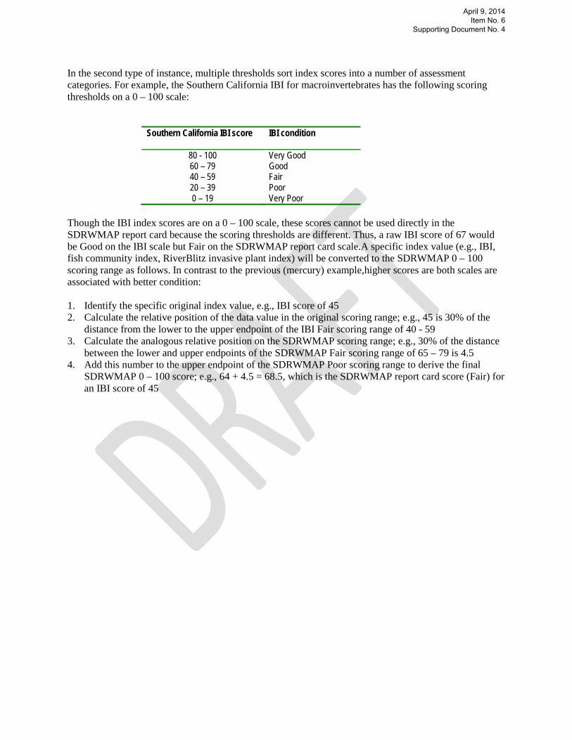
In the second type of instance, multiple thresholds sort index scores into a number of assessment categories. For example, the Southern California IBI for macroinvertebrates has the following scoring thresholds on a 0 – 100 scale:

Southern California IBI score

IBI condition

80 - 100 Very Good 60 – 79 Good 40 – 59 Fair 20 – 39 Poor 0 – 19 Very Poor

Though the IBI index scores are on a 0 – 100 scale, these scores cannot be used directly in the SDRWMAP report card because the scoring thresholds are different. Thus, a raw IBI score of 67 would be Good on the IBI scale but Fair on the SDRWMAP report card scale.A specific index value (e.g., IBI, fish community index, RiverBlitz invasive plant index) will be converted to the SDRWMAP 0 – 100 scoring range as follows. In contrast to the previous (mercury) example,higher scores are both scales are associated with better condition: 1. Identify the specific original index value, e.g., IBI score of 45 2. Calculate the relative position of the data value in the original scoring range; e.g., 45 is 30% of the

distance from the lower to the upper endpoint of the IBI Fair scoring range of 40 - 59 3. Calculate the analogous relative position on the SDRWMAP scoring range; e.g., 30% of the distance

between the lower and upper endpoints of the SDRWMAP Fair scoring range of 65 – 79 is 4.5 4. Add this number to the upper endpoint of the SDRWMAP Poor scoring range to derive the final

SDRWMAP 0 – 100 score; e.g., 64 + 4.5 = 68.5, which is the SDRWMAP report card score (Fair) for an IBI score of 45



Documents

SAN DIEGO RIVER WATERSHED MONITORING AND …