SANDIA REPORTSAND2002-1320Unlimited ReleasePrinted May 2002

Sandia Smart Anti-Islanding Project Summer 2001

Task IIInvestigation of the Impact of Single-phase InductionMachines in Islanded Loads

Summary of ResultsMike Ropp, Russell Bonn, Sigifredo Gonzalez, and Chuck Whitaker

Prepared bySandia National LaboratoriesAlbuquerque, New Mexico 87185 and Livermore, California 94550

Sandia is a multiprogram laboratory operated by Sandia Corporation,a Lockheed Martin Company, for the United States Department ofEnergy under Contract DE-AC04-94AL85000.

Approved for public release; further dissemination unlimited.

Issued by Sandia National Laboratories, operated for the United States Departmentof Energy by Sandia Corporation.

NOTICE: This report was prepared as an account of work sponsored by an agencyof the United States Government. Neither the United States Government, nor anyagency thereof, nor any of their employees, nor any of their contractors,subcontractors, or their employees, make any warranty, express or implied, orassume any legal liability or responsibility for the accuracy, completeness, orusefulness of any information, apparatus, product, or process disclosed, or representthat its use would not infringe privately owned rights. Reference herein to anyspecific commercial product, process, or service by trade name, trademark,manufacturer, or otherwise, does not necessarily constitute or imply its endorsement,recommendation, or favoring by the United States Government, any agency thereof,or any of their contractors or subcontractors. The views and opinions expressedherein do not necessarily state or reflect those of the United States Government, anyagency thereof, or any of their contractors.

Printed in the United States of America. This report has been reproduced directlyfrom the best available copy.

Available to DOE and DOE contractors fromU.S. Department of EnergyOffice of Scientific and Technical InformationP.O. Box 62Oak Ridge, TN 37831

Telephone: (865)576-8401Facsimile: (865)576-5728E-Mail: reports@adonis.osti.govOnline ordering: http://www.doe.gov/bridge

Available to the public fromU.S. Department of CommerceNational Technical Information Service5285 Port Royal RdSpringfield, VA 22161

Telephone: (800)553-6847Facsimile: (703)605-6900E-Mail: orders@ntis.fedworld.govOnline order: http://www.ntis.gov/ordering.htm

3

SAND2002-1320Unlimited ReleasePrinted May 2002

Sandia Smart Anti-Islanding ProjectSummer 2001

Task IIInvestigation of the Impact of Single-phase

Induction Machines in Islanded Loads

Summary of Results

Mike RoppSouth Dakota State University

Brookings, SD 57007

Russell Bonn and Sigifredo GonzalezPhotovoltaic Systems

Sandia National LaboratoriesP. O. Box 5800

Albuquerque, NM 87185-0753

Chuck WhitakerEndecon Engineering

San Ramon, CA 94583

ABSTRACT

Islanding, the supply of energy to a disconnected portion of the grid, is a phenomenon that couldresult in personnel hazard, interfere with reclosure, or damage hardware. Considerable effort hasbeen expended on the development of IEEE 929, a document that defines unacceptable islandingand a method for evaluating energy sources. The worst expected loads for an islanded inverterare defined in IEEE 929 as being composed of passive resistance, inductance, and capacitance.However, a controversy continues concerning the possibility that a capacitively compensated,single-phase induction motor with a very lightly damped mechanical load having a largerotational inertia would be a significantly more difficult load to shed during an island. This reportdocuments the result of a study that shows such a motor is not a more severe case, simply aspecial case of the RLC network.

4

Table of Contents

Introduction . . . . . . . . . . . . . . . . . . . . . . . . . . . . . . . . . . . . . . . . . . . . . . . . . . . . . . . . . . . . 5

Procedure . . . . . . . . . . . . . . . . . . . . . . . . . . . . . . . . . . . . . . . . . . . . . . . . . . . . . . . . . . . . . 7

Results . . . . . . . . . . . . . . . . . . . . . . . . . . . . . . . . . . . . . . . . . . . . . . . . . . . . . . . . . . . . . . . . 14

Discussion . . . . . . . . . . . . . . . . . . . . . . . . . . . . . . . . . . . . . . . . . . . . . . . . . . . . . . . . . . . . . 17

Experimental Verification of Results . . . . . . . . . . . . . . . . . . . . . . . . . . . . . . . . . . . . . . . . 17

Conclusion . . . . . . . . . . . . . . . . . . . . . . . . . . . . . . . . . . . . . . . . . . . . . . . . . . . . . . . . . . . . . 21

References . . . . . . . . . . . . . . . . . . . . . . . . . . . . . . . . . . . . . . . . . . . . . . . . . . . . . . . . . . . . . 22

Appendix A . . . . . . . . . . . . . . . . . . . . . . . . . . . . . . . . . . . . . . . . . . . . . . . . . . . . . . . . . . . . 23

5

Introduction

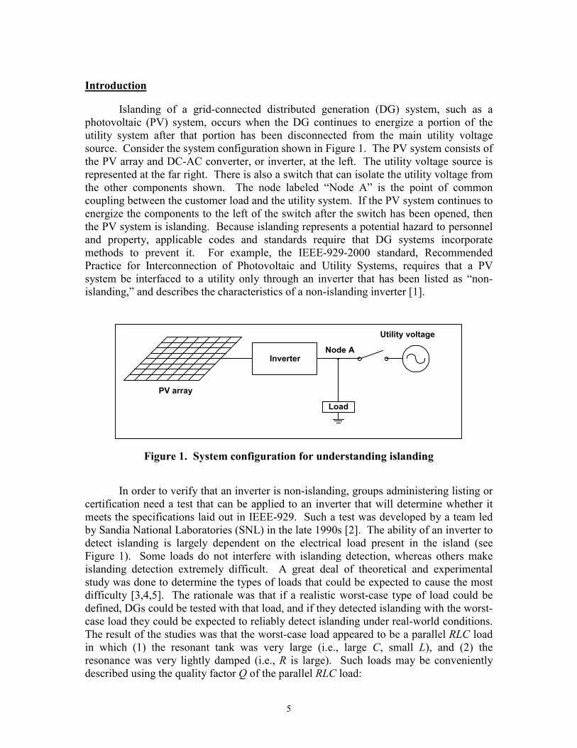
Islanding of a grid-connected distributed generation (DG) system, such as aphotovoltaic (PV) system, occurs when the DG continues to energize a portion of theutility system after that portion has been disconnected from the main utility voltagesource. Consider the system configuration shown in Figure 1. The PV system consists ofthe PV array and DC-AC converter, or inverter, at the left. The utility voltage source isrepresented at the far right. There is also a switch that can isolate the utility voltage fromthe other components shown. The node labeled “Node A” is the point of commoncoupling between the customer load and the utility system. If the PV system continues toenergize the components to the left of the switch after the switch has been opened, thenthe PV system is islanding. Because islanding represents a potential hazard to personneland property, applicable codes and standards require that DG systems incorporatemethods to prevent it. For example, the IEEE-929-2000 standard, RecommendedPractice for Interconnection of Photovoltaic and Utility Systems, requires that a PVsystem be interfaced to a utility only through an inverter that has been listed as “non-islanding,” and describes the characteristics of a non-islanding inverter [1].

Figure 1. System configuration for understanding islanding

In order to verify that an inverter is non-islanding, groups administering listing orcertification need a test that can be applied to an inverter that will determine whether itmeets the specifications laid out in IEEE-929. Such a test was developed by a team ledby Sandia National Laboratories (SNL) in the late 1990s [2]. The ability of an inverter todetect islanding is largely dependent on the electrical load present in the island (seeFigure 1). Some loads do not interfere with islanding detection, whereas others makeislanding detection extremely difficult. A great deal of theoretical and experimentalstudy was done to determine the types of loads that could be expected to cause the mostdifficulty [3,4,5]. The rationale was that if a realistic worst-case type of load could bedefined, DGs could be tested with that load, and if they detected islanding with the worst-case load they could be expected to reliably detect islanding under real-world conditions.The result of the studies was that the worst-case load appeared to be a parallel RLC loadin which (1) the resonant tank was very large (i.e., large C, small L), and (2) theresonance was very lightly damped (i.e., R is large). Such loads may be convenientlydescribed using the quality factor Q of the parallel RLC load:

InverterNode A

Load

Utility voltage

PV array

6

L

CRQ � [1]

The worst-case RLC load described above corresponds to a load with a high value of Q,and a resonant frequency within the DG’s under- and over-frequency trip setpoints. (It isimportant to note that both conditions are important; an extremely high-Q load with itsresonant frequency outside the trip setpoints of the DG will not lead to long run-ontimes.) With such a load, the time between disconnection of the utility and the time atwhich the PV inverter detects islanding and discontinues operation, known as the run-ontime, could be very long, or even indefinitely long. Thus, SNL personnel specified a testusing this type of parallel RLC load.

As might be expected, further experimentation raised further questions. Oneparticularly troubling question arose repeatedly: Experimenters were inconsistentlyobserving that they could get very long run-on times if, instead of using the worst-caseparallel RLC load, they used a load containing a capacitively compensated, single-phaseinduction motor with a very lightly damped mechanical load that had a large rotationalinertia [2,6]. The most common realization of this type of load was a bench grinder, amotor driving one or more large stone grinding wheels acting as flywheels.

A proposed explanation for this phenomenon was that the flywheel, whose timeconstant is several orders of magnitude slower than that of the electrical system, could actas a prime mover during the electrical transient. It’s rotational inertia could turn theinduction machine as a generator, sending its kinetic energy into the island andmaintaining the voltage that causes the PV system to continue operating. However,theory suggested that this was not possible. In order for the single-phase inductionmachine to act as a generator, assuming the rotational speed to be held constant by thelarge rotational inertia, it would be necessary for the electrical frequency in the island tochange. According to the basic theory described below, under practical conditions, asingle-phase induction motor generally cannot reach its generator range of operationwithout reaching the under-frequency trip setpoint of the PV system, causing it to trip offline.

However, the question remained as to why longer run-on times were being seenwith motors than with the RLC loads. In fact, this question was sufficiently troubling tosome standards-making bodies that they proposed to include motors in the loads used totest non-islanding inverters. This solution presents extreme logistical problems withreproducibility, as it is difficult to make certain all certifying organizations use the“same” motor. Even specifying the “standard” motor for use in the tests would bedifficult as there is such a wide range of motor sizes and types in use.

As these difficulties became apparent, SNL initiated a study to determine whetherin fact the induction machine represented a worst-case load, and thus whether it wasnecessary to include motors in test loads. This document describes the results of thisstudy.

7

Procedure

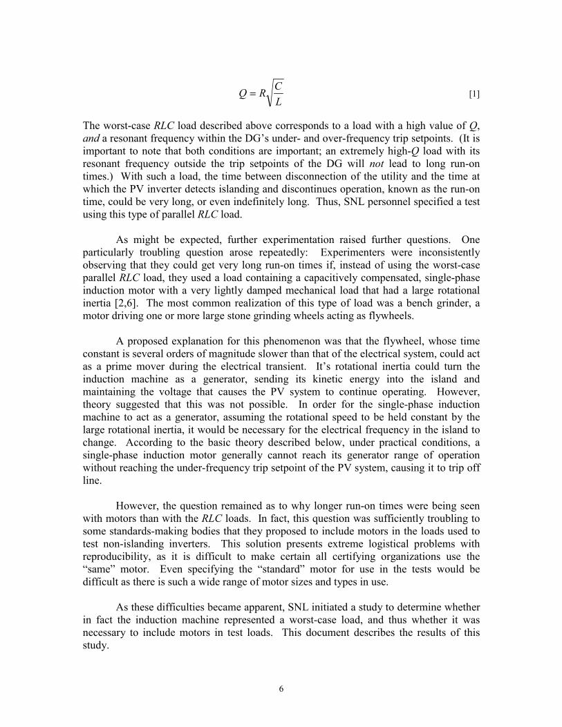
As described above, theory suggests that the explanation that the motor is actingas a generator is not possible because of the physics of the induction machine. Tounderstand why this is so, consider the electrical schematic of the single-phase inductionmachine shown in Figure 2 [7].

Figure 2. Schematic of a single-phase induction machine [7]

The voltage Vin applied to the terminals of the machine is the motor’s driving voltage.The various electrical, magnetic, and mechanical mechanisms within the machine may berepresented by the combination of inductors and resistors shown. The values of resistorsRY and RZ are functions of the mechanical load on the machine (and a variety of otherfactors) through a parameter known as the slip. The slip S is defined as

[2]

where the electrical synchronous frequency is proportional to the frequency of the appliedvoltage Vin (it is the frequency of Vin divided by the number of magnetic pole pairs in themachine), and the mechanical frequency is the rotational frequency of the machine andload (assuming no gears). Note that the slip is always less than 1. Typically, for a single-phase machine under steady-state, 60 Hz operation, S is on the order of 0.05. The torqueproduced by the machine is in part a function of the slip, and in this way the steady-stateoperating value of the slip depends on the mechanical load.

The relationships between RY and RZ and the slip are [7]:

L1R1

LW

LX

LY

LZ

RY

RZ

+

Vin

-

� � � �� �frequency ssynchronou electrical

frequency mechanicalfrequency ssynchronou electrical �

�S

8

[3]

[4]

where R is a constant for a specific machine. Thus, since S depends on the electrical andmechanical frequencies, the resistances RY and RZ are also functions of the electrical andmechanical frequencies.

In the present case in which the rotational inertia of the load is very large, themechanical frequency can be considered to be constant over time periods of interest.Thus, S, RY and RZ depend on electrical frequency only. In order for the machinerepresented in Figure 2 to enter the generator mode of operation, the resistance RY mustbecome negative, and Equation 3 clearly shows that the only way for this to occur, sinceR is positive, is for S to become negative. According to Equation 2, since the mechanicalfrequency is (approximately) constant in our case, there must be a decrease in electricalfrequency to obtain generation. If we assume 60 Hz electrical excitation and a slip of0.05, then the frequency at which the slip becomes zero would be 57 Hz, and must dropbelow that to obtain generation. Since IEEE-929-2000 already requires PV inverters totrip off line if the frequency drops below 59.3 Hz, this condition clearly would bedetected by the inverter. This is the reason for the previous statement that theorysuggests that the induction machine cannot be causing longer run-on times throughgeneration.

What, then, is the reason for the experimental observation of longer run-on timeswith induction motors? As mentioned in the Introduction, it is well known now that thelarger the value of Q of an RLC circuit is (i.e., the larger the energy stored in the resonantcircuit is relative to what is dissipated), the longer the run-on times will be, provided thatthe load’s resonant frequency is within the DG’s frequency trip setpoints. The inductiveenergy storage in an induction machine is typically very large (the equivalent value of Lis small), and the value of capacitance C required to compensate it is large. This meansthat a motor load can be thought of as a practical way to realize the high-Q “RLC” loadalready known to be a worst case for islanding detection. (“RLC” is placed in quotesbecause the motor load is not a parallel RLC circuit.) In fact, an examination of some ofthe earlier results [2,6] indicates that when the experimenters compared motor and RLCloads, the values of capacitance used in the motor load cases were three or more timeslarger than that used in the RLC loads. Thus, the postulate proposed here is that in factthe rotating load has little or nothing to do with the extended run-on times observed.Rather, they are caused by the fact that the capacitively compensated motor loadconveniently realizes a more severe case of the already known worst-case high-Q RLCload.

To test this theory, the following procedure was adopted. First, computersimulations were used to test “equivalent” motor and RLC loads. Equivalent loads are

� �S

RR

S

RR

Z

Y

�

�

�

22

2

9

defined as loads that have identical complex impedances; that is, the compleximpedances presented to the utility and DG by the equivalent loads will be the same. Thecomputer simulated a utility with its impedance, either an RLC or capacitivelycompensated induction machine load, and a DG (considered herein to be a photovoltaic[PV] system) equipped with the Sandia Frequency Shift (SFS) method of islandingdetection. Simulations were run with loads including capacitors closely matched to theresonant value, and the behavior of the PV system was quantified by plotting thefrequency of the voltage at Node A in Figure 1. The frequency trajectories of the systemwith the different loads were compared to determine whether there is a significantdifference between the system’s behavior with the different loads.

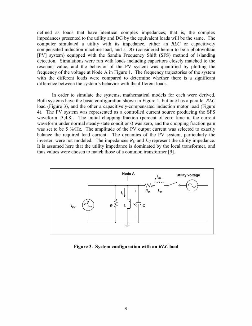
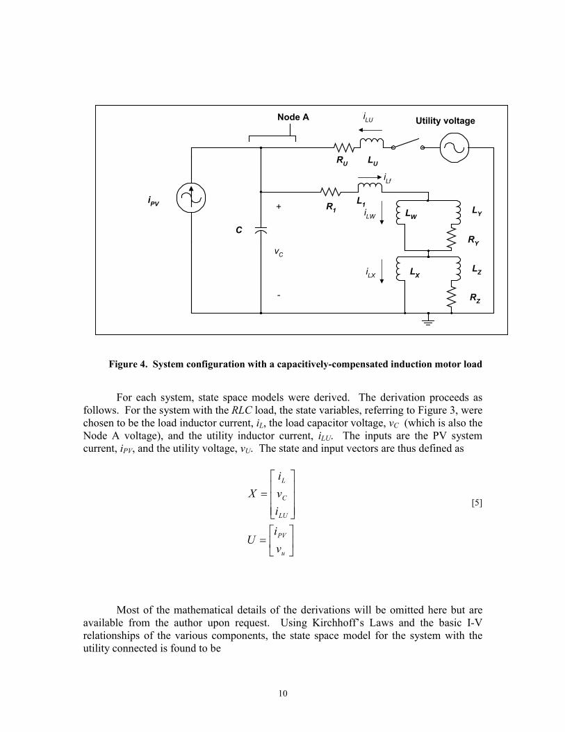
In order to simulate the systems, mathematical models for each were derived.Both systems have the basic configuration shown in Figure 1, but one has a parallel RLCload (Figure 3), and the other a capacitively-compensated induction motor load (Figure4). The PV system was represented as a controlled current source producing the SFSwaveform [3,4,8]. The initial chopping fraction (percent of zero time in the currentwaveform under normal steady-state conditions) was zero, and the chopping fraction gainwas set to be 5 %/Hz. The amplitude of the PV output current was selected to exactlybalance the required load current. The dynamics of the PV system, particularly theinverter, were not modeled. The impedances RU and LU represent the utility impedance.It is assumed here that the utility impedance is dominated by the local transformer, andthus values were chosen to match those of a common transformer [9].

Figure 3. System configuration with an RLC load

Node A Utility voltage

iPV R L C

RU LUiL+

vC

-

iLU

10

Figure 4. System configuration with a capacitively-compensated induction motor load

For each system, state space models were derived. The derivation proceeds asfollows. For the system with the RLC load, the state variables, referring to Figure 3, werechosen to be the load inductor current, iL, the load capacitor voltage, vC (which is also theNode A voltage), and the utility inductor current, iLU. The inputs are the PV systemcurrent, iPV, and the utility voltage, vU. The state and input vectors are thus defined as

[5]

Most of the mathematical details of the derivations will be omitted here but areavailable from the author upon request. Using Kirchhoff’s Laws and the basic I-Vrelationships of the various components, the state space model for the system with theutility connected is found to be

Node A Utility voltage

iPV

C

RU LU

L1R1 LW

LX

LY

LZ

RY

RZ

+

vC

-

iLU

iLW

iLX

iLf

��

���

��

���

�

�

���

�

�

�

u

PV

LU

C

L

v

iU

i

v

i

X

11

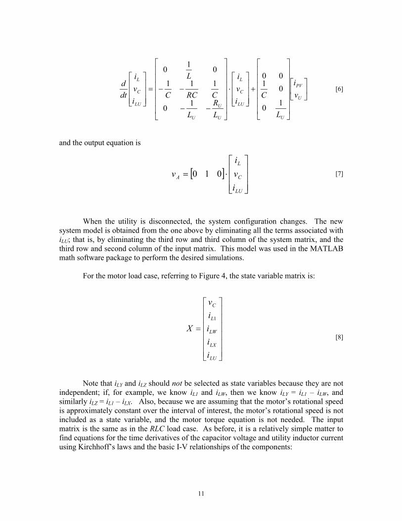
[6]

and the output equation is

[7]

When the utility is disconnected, the system configuration changes. The newsystem model is obtained from the one above by eliminating all the terms associated withiLU; that is, by eliminating the third row and third column of the system matrix, and thethird row and second column of the input matrix. This model was used in the MATLABmath software package to perform the desired simulations.

For the motor load case, referring to Figure 4, the state variable matrix is:

[8]

Note that iLY and iLZ should not be selected as state variables because they are notindependent; if, for example, we know iL1 and iLW, then we know iLY = iL1 – iLW, andsimilarly iLZ = iL1 – iLX. Also, because we are assuming that the motor’s rotational speedis approximately constant over the interval of interest, the motor’s rotational speed is notincluded as a state variable, and the motor torque equation is not needed. The inputmatrix is the same as in the RLC load case. As before, it is a relatively simple matter tofind equations for the time derivatives of the capacitor voltage and utility inductor currentusing Kirchhoff’s laws and the basic I-V relationships of the components:

��

���

�

������

�

�

������

�

�

�

���

�

�

���

�

�

�

������

�

�

������

�

�

���

�

�

���

�

�

U

PV

U

LU

C

L

U

U

U

LU

C

L

v

i

L

Ci

v

i

L

R

L

CRCC

L

i

v

i

dt

d

10

0100

10

111

010

� ����

�

�

���

�

�

��

LU

C

L

A

i

v

i

v 010

������

�

�

������

�

�

�

LU

LX

LW

L

C

i

i

i

i

v

X1

12

[9]

[10]

Finding equations for the time derivatives of the other three state variables isslightly more complicated. If we use the basic relationships as before, we can find threeequations in three unknowns (namely the three desired time derivatives). If Kirchhoff’sVoltage Law is applied to a loop containing C, R1, LW, and LX, and also around the twoclosed R-L loops in the induction motor model, and the above-noted expressions for iLY

and iLZ are used, the following equations are obtained.

[11]

[12]

[13]

We now have a set of five equations in the five unknowns in our system:

[14]

This equation is not in the standard form for state space systems, which is

However, it can be put into the standard form easily if the matrix M1 is invertible, whichit is in the present case. Thus we premultiply both sides of the equation by M1

-1 andidentify

BUAXdt

dX��

UU

LUU

UC

U

LU

PVLULc

vL

iL

Rv

Ldt

di

iC

iC

iCdt

dv

11

1111

����

����

� � � �

� � � �LXLZL

ZLX

ZX

LWLYL

YLW

YW

LcLX

XLW

WL

iiRdt

diL

dt

diLL

iiRdt

diL

dt

diLL

Rivdt

diL

dt

diL

dt

diL

����

����

����

11

11

111

1

������

�

�

������

�

�

�

������

�

�

������

�

�

��

�

�

�

�

�

������

�

�

������

�

�

�

��

�

1000000001

;

0001000000000110010

;

0000000000000000

3

1

2

1

1

321

M

R

RR

RR

R

M

L

LLL

LLL

LLL

C

M

UMXMdt

dXM

U

YY

ZZ

U

YWY

ZXZ

XW

13

This completes the derivation.

In order to find the capacitor that exactly compensates the motor load to a unitypower factor (i.e., such that the imaginary part of the compensated motor’s impedance iszero), an expression for the imaginary part of the compensated motor impedance wasderived. The impedance of the motor is

[15]

where � is the electrical frequency in radians per second. This complex impedance x +jy is in parallel with the compensating capacitor impedance:

[16]

The imaginary part of Zload is then isolated and set equal to zero (for a unity power factorload), and solved for C = Cres, the resonant capacitance. After considerablemanipulation, the result is

[17]

Once the motor parameters are chosen, the values of x and y can be found easily inMATLAB, and the compensating Cres can be calculated using Equation 17.

To find the RLC load equivalent to the given motor load, the real and imaginaryparts of the RLC load must be equivalent to those of the motor load. First, the value of Lcan be calculated because the value of Cres is already known, and

[18]

The real part of the RLC load will be determined by R and must be set equal to thereal part of the compensated motor load.

31

1

21

1

MMB

MMA�

�

�

�

jyx

LjRLjLjRLjLjRZ

ZZXYYWmotor

��

��

���

�

����

�

���

�

����

�� 11

111111����

�

� �jyxCjZCjZ

motor

load

��

�

�

�

11

11

��

� � resCyx

yC �

�

� 22�

resCL 2

1�

�

14

Having derived the needed state-space models, MATLAB programs were writtento simulate both system configurations. The motor and RLC load parameters used areincluded in Appendix A at the end of this document. (The reader is encouraged to notethat, as previously mentioned, choosing a “typical” set of induction motor parameters isextremely difficult because of the wide range of values possible in practice. The setselected here represents a “reasonable” set from the literature.) Simulations were runwith several values of C, all near to Cres but slightly different so that the frequencybehavior can be seen. (If a value exactly equal to Cres is used, there should be practicallyzero frequency deviation in either case.) Thus, the resonant frequency of the circuit isalways within the frequency trip limits of the DG. The Q factors of the RLC loads usedhere are all � 2, ranging from about 1.800 to 2.006. The DG is modeled as a controllablecurrent source operating at unity power factor. A negative-to-positive zero crossingdetector detected the rising zero crossings of the Node A voltage. When such a crossingis detected, the frequency is calculated using the time since the previous zero crossing.The measured frequency is stored for plotting and is also used to dynamically recomputethe motor slip using Equation 1.

Results

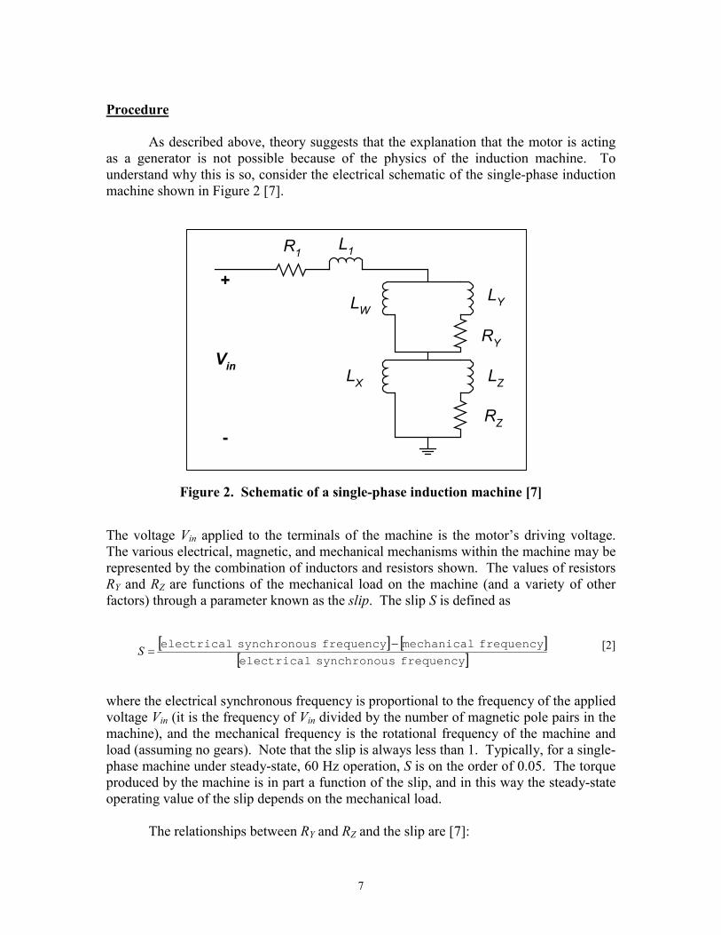
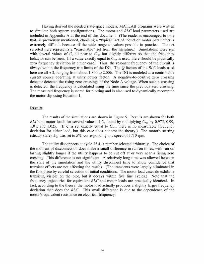
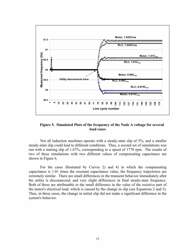
The results of the simulations are shown in Figure 5. Results are shown for bothRLC and motor loads for several values of C, found by multiplying Cres by 0.975, 0.99,1.01, and 1.025. (If C is set exactly equal to Cres, there is no measurable frequencydeviation for either load, but this case does not test the theory.) The motor's starting(steady-state) slip was set to 5%, corresponding to a speed of 1710 rpm.

The utility disconnects at cycle 75.4, a number selected arbitrarily. The choice ofthe moment of disconnection does make a small difference in run-on times, with run-onlasting slightly longer if the utility happens to be cut off at or very near a rising zerocrossing. This difference is not significant. A relatively long time was allowed betweenthe start of the simulation and the utility disconnect time to allow confidence thattransient effects are not affecting the results. (The transients were largely eliminated inthe first place by careful selection of initial conditions. The motor load cases do exhibit atransient, visible on the plot, but it decays within five line cycles.) Note that thefrequency trajectories for equivalent RLC and motor loads are practically identical. Infact, according to the theory, the motor load actually produces a slightly larger frequencydeviation than does the RLC. This small difference is due to the dependence of themotor’s equivalent resistance on electrical frequency.

15

Figure 5. Simulated Plots of the frequency of the Node A voltage for severalload cases

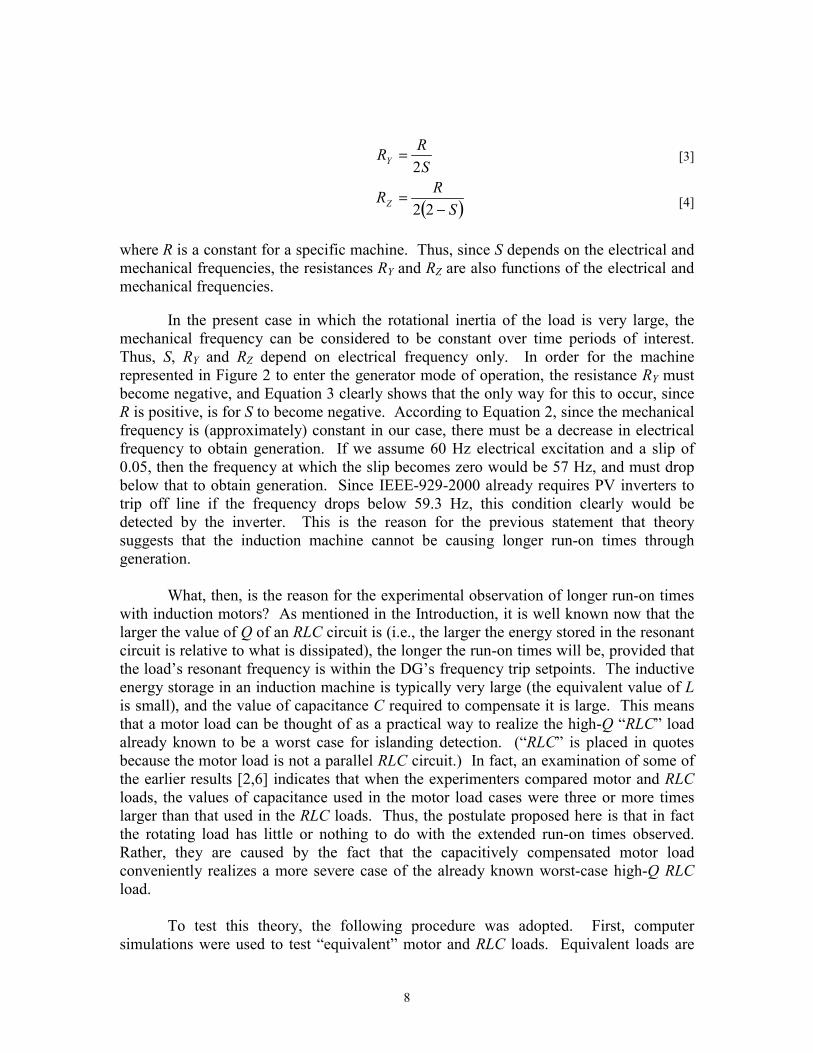
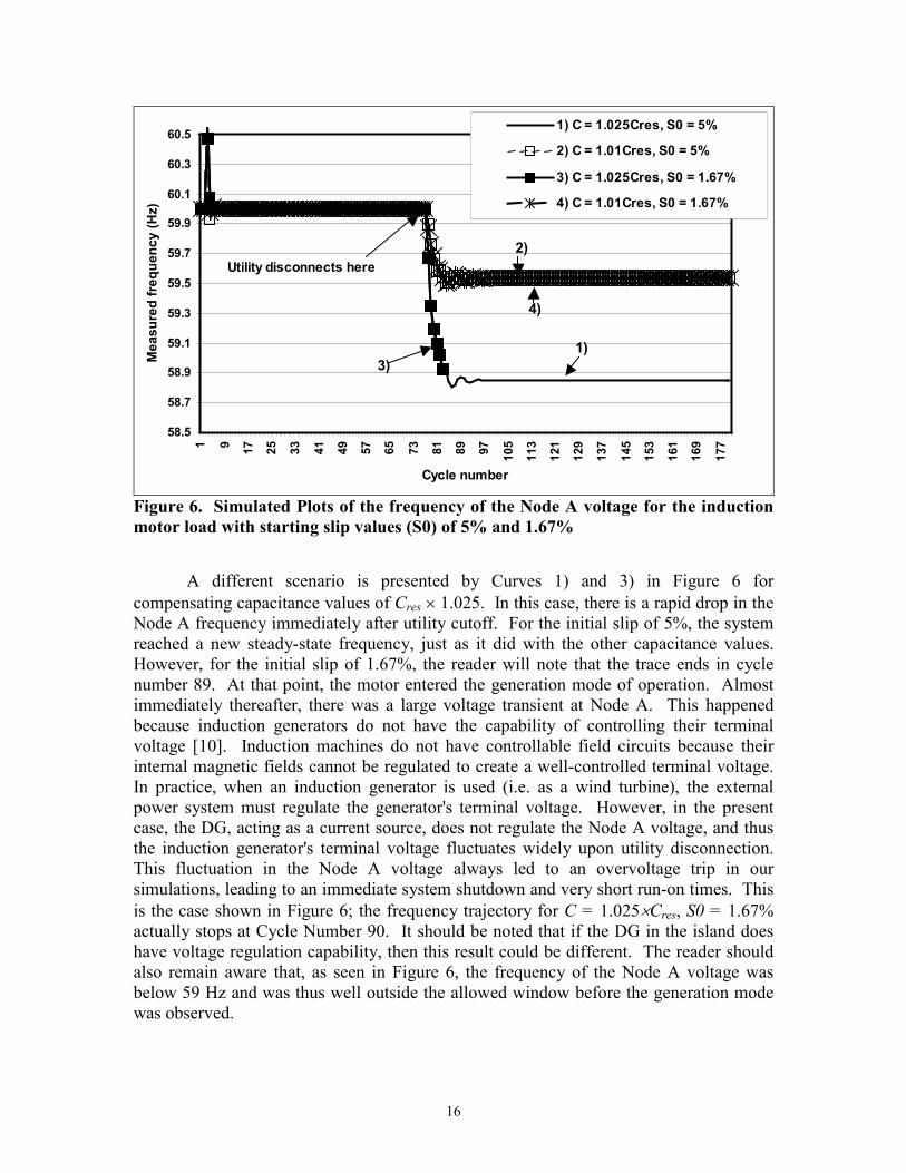
Not all induction machines operate with a steady-state slip of 5%, and a smallersteady-state slip could lead to different conditions. Thus, a second set of simulations wasrun with a starting slip of 1.67%, corresponding to a speed of 1770 rpm. The results oftwo of these simulations with two different values of compensating capacitance areshown in Figure 6.

For the cases illustrated by Curves 2) and 4) in which the compensatingcapacitance is 1.01 times the resonant capacitance value, the frequency trajectories areextremely similar. There are small differences in the transient behavior immediately afterthe utility is disconnected, and very slight differences in final steady-state frequency.Both of these are attributable to the small difference in the value of the resistive part ofthe motor's electrical load, which is caused by the change in slip (see Equations 2 and 3).Thus, in these cases, the change in initial slip did not make a significant difference in thesystem's behavior.

58.5

59

59.5

60

60.5

61

61.5

1 8 15 22 29 36 43 50 57 64 71 78 85 92 99 106

113

120

127

134

141

148

155

162

169

176

Line cycle number

Mea

sure

d fr

eque

ncy

(Hz)

Motor, 1.025Cres

RLC, 1.025Cres

Motor, 1.01Cres

RLC, 1.01Cres

RLC, 0.99Cres

Motor, 0.99Cres

RLC, 0.975Cres

Motor, 0.975Cres

Utility disconnects here

16

58.5

58.7

58.9

59.1

59.3

59.5

59.7

59.9

60.1

60.3

60.5

1 9 17 25 33 41 49 57 65 73 81 89 97 105

113

121

129

137

145

153

161

169

177

Cycle number

Mea

sure

d fr

eque

ncy

(Hz)

1) C = 1.025Cres, S0 = 5%

2) C = 1.01Cres, S0 = 5%

3) C = 1.025Cres, S0 = 1.67%

4) C = 1.01Cres, S0 = 1.67%

Utility disconnects here

3)1)

2)

4)

Figure 6. Simulated Plots of the frequency of the Node A voltage for the inductionmotor load with starting slip values (S0) of 5% and 1.67%

A different scenario is presented by Curves 1) and 3) in Figure 6 forcompensating capacitance values of Cres � 1.025. In this case, there is a rapid drop in theNode A frequency immediately after utility cutoff. For the initial slip of 5%, the systemreached a new steady-state frequency, just as it did with the other capacitance values.However, for the initial slip of 1.67%, the reader will note that the trace ends in cyclenumber 89. At that point, the motor entered the generation mode of operation. Almostimmediately thereafter, there was a large voltage transient at Node A. This happenedbecause induction generators do not have the capability of controlling their terminalvoltage [10]. Induction machines do not have controllable field circuits because theirinternal magnetic fields cannot be regulated to create a well-controlled terminal voltage.In practice, when an induction generator is used (i.e. as a wind turbine), the externalpower system must regulate the generator's terminal voltage. However, in the presentcase, the DG, acting as a current source, does not regulate the Node A voltage, and thusthe induction generator's terminal voltage fluctuates widely upon utility disconnection.This fluctuation in the Node A voltage always led to an overvoltage trip in oursimulations, leading to an immediate system shutdown and very short run-on times. Thisis the case shown in Figure 6; the frequency trajectory for C = 1.025�Cres, S0 = 1.67%actually stops at Cycle Number 90. It should be noted that if the DG in the island doeshave voltage regulation capability, then this result could be different. The reader shouldalso remain aware that, as seen in Figure 6, the frequency of the Node A voltage wasbelow 59 Hz and was thus well outside the allowed window before the generation modewas observed.

17

Discussion

The simulations suggest that the explanation proposed here is correct; theextended run-on times observed for single-phase induction motor loads in the past arecaused by the fact that the motor load conveniently represents an analog to the already-known worst case load for islanding prevention, the high-Q parallel RLC circuit withresonant frequency very near the line frequency. Furthermore, it appears that if theinduction machine were to enter the generation mode, the possibility of islanding wouldactually be reduced due to the lack of voltage regulation in the island, unless the DG inuse has voltage regulation capability. It must be borne in mind that this simulation doesneglect the variation of motor rotational speed with changing electrical frequency. Aftera time, the rotational speed will change slightly, reaching a new value determined by therequired load torque and the motor characteristics. However, over the frequency rangeshown here, this change would be very small and probably too small to affect the basicresult.

A brief discussion of the extension of these results to larger DGs feeding three-phase induction machines is in order at this point. The development here hasconcentrated on single-phase machines because these are the type used in virtually all ofthe experiments to date. However, three-phase machines have an equivalent circuit thatis similar to that of the single-phase machine in that there is a resistance value thatdepends on slip, and the machine cannot enter the generation mode unless the slipbecomes negative [7, 11]. Therefore, the basic behavior of the three-phase system, interms of islanding prevention, should not be significantly different than that of the single-phase system presented here. In other words, the three-phase motor may also besufficiently modeled by a three-phase RLC load. One potential difference between thethree-phase and single-phase cases is that three-phase motors, in general, tend to operateat lower slip values. Thus, the case in which the generator mode is seen could be moreprevalent for three-phase machines.

Experimental Verification of Results

Simulation cannot replace experimentation. Therefore, the following experimentwas performed at SNL to verify the simulation results. The DG, a PV system, used theSFS islanding prevention method for maximum compatibility with the simulation results.Note, however, that this was not necessary, as the fundamental conclusion reached aboveis independent of the islanding prevention method used.

Part I

(1) The first load to be tested was a 1/2-horsepower bench grinder driven by a single-phase induction machine. The grinder was not mechanically loaded (i.e. thegrinding wheels were allowed to spin freely). The complex impedance of themotor was determined by applying 60 Hz power to the motor, allowing it to cometo steady state, and using a power meter to characterize the current drawn by the

18

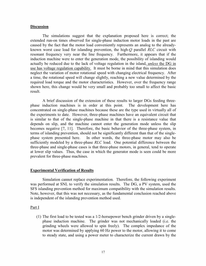
motor. The results of these measurements, without capacitive compensation, aregiven in Table 1. The current waveform drawn by the uncompensated motor isshown in Figure 7. Note that there is a small amount of distortion (almost 6%THD, as given in Table 1).

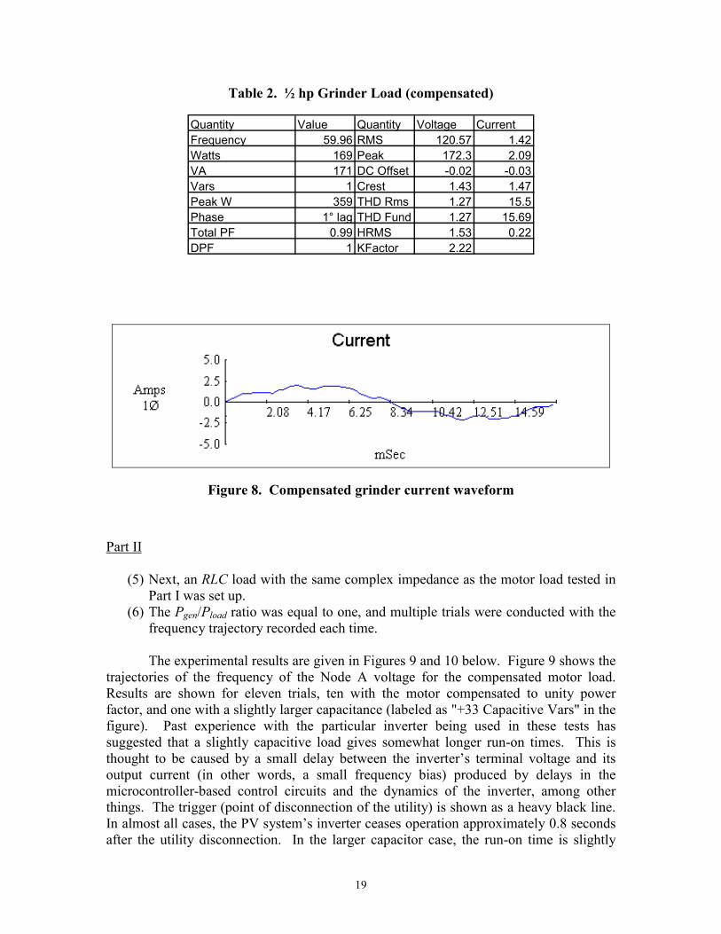
(2) The motor was then capacitively compensated to nearly unity power factor at 60Hz, and the characterization measurements were repeated on the compensatedmotor. The results of these measurements are given in Table 2. The level ofdistortion in the current was higher in this case, as indicated by the THDmeasurements in Table 2 and the plot of the compensated motor current in Figure8. (This is important because it has been previously shown [3] that nonlinearitiesin local loads should lead to shorter run-on times.)

(3) The ratio of DG input power to load power, Pgen/Pload, was set equal to one.(4) Multiple tests were conducted, and the frequency trajectory of the Node A voltage

was recorded each time. In some of the trials, the size of the capacitor was setslightly larger than the resonant value, so that the capacitor was supplying slightlymore reactive power (VARs) than the load required. Past experience has shownthis to lead to slightly longer run-on times, probably because of a slight time delaybetween the DG's output current waveform and the Node A voltage which iscompensated by the slightly larger capacitance.

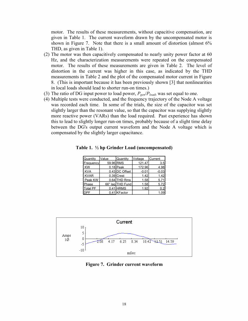
Table 1. ½ hp Grinder Load (uncompensated)

Quantity Value Quantity Voltage CurrentFrequency 59.96 RMS 121.47 3.5 KW 0.18 Peak 172.96 4.98 KVA 0.43 DC Offset -0.01 -0.03 KVAR 0.39 Crest 1.42 1.42 Peak KW 0.64 THD Rms 1.58 5.71Phase 66° lag THD Fund 1.58 5.72Total PF 0.41 HRMS 1.92 0.2DPF 0.41 KFactor 1.09

Figure 7. Grinder current waveform

19

Table 2. ½ hp Grinder Load (compensated)

Quantity Value Quantity Voltage CurrentFrequency 59.96 RMS 120.57 1.42Watts 169 Peak 172.3 2.09VA 171 DC Offset -0.02 -0.03Vars 1 Crest 1.43 1.47Peak W 359 THD Rms 1.27 15.5Phase 1° lag THD Fund 1.27 15.69Total PF 0.99 HRMS 1.53 0.22DPF 1 KFactor 2.22

Figure 8. Compensated grinder current waveform

Part II

(5) Next, an RLC load with the same complex impedance as the motor load tested inPart I was set up.

(6) The Pgen/Pload ratio was equal to one, and multiple trials were conducted with thefrequency trajectory recorded each time.

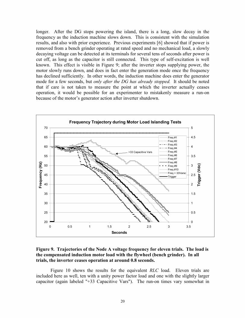
The experimental results are given in Figures 9 and 10 below. Figure 9 shows thetrajectories of the frequency of the Node A voltage for the compensated motor load.Results are shown for eleven trials, ten with the motor compensated to unity powerfactor, and one with a slightly larger capacitance (labeled as "+33 Capacitive Vars" in thefigure). Past experience with the particular inverter being used in these tests hassuggested that a slightly capacitive load gives somewhat longer run-on times. This isthought to be caused by a small delay between the inverter’s terminal voltage and itsoutput current (in other words, a small frequency bias) produced by delays in themicrocontroller-based control circuits and the dynamics of the inverter, among otherthings. The trigger (point of disconnection of the utility) is shown as a heavy black line.In almost all cases, the PV system’s inverter ceases operation approximately 0.8 secondsafter the utility disconnection. In the larger capacitor case, the run-on time is slightly

20

longer. After the DG stops powering the island, there is a long, slow decay in thefrequency as the induction machine slows down. This is consistent with the simulationresults, and also with prior experience. Previous experiments [6] showed that if power isremoved from a bench grinder operating at rated speed and no mechanical load, a slowlydecaying voltage can be detected at its terminals for several tens of seconds after power iscut off, as long as the capacitor is still connected. This type of self-excitation is wellknown. This effect is visible in Figure 9; after the inverter stops supplying power, themotor slowly runs down, and does in fact enter the generation mode once the frequencyhas declined sufficiently. In other words, the induction machine does enter the generatormode for a few seconds, but only after the DG has already stopped. It should be notedthat if care is not taken to measure the point at which the inverter actually ceasesoperation, it would be possible for an experimenter to mistakenly measure a run-onbecause of the motor’s generator action after inverter shutdown.

Frequency Trajectory during Motor Load Islanding Tests

20

25

30

35

40

45

50

55

60

65

70

0 0.5 1 1.5 2 2.5 3 3.5

Seconds

Freq

uenc

y (H

z)

0

0.5

1

1.5

2

2.5

3

3.5

4

4.5

5

Trig

ger (

Vdc)

Freq #1Freq #2Freq #3Freq #4Freq #5Freq #6Freq #7Freq #8Freq #9Freq #10Freq + 33VarscTrigger

+33 Capacitive Vars

Figure 9. Trajectories of the Node A voltage frequency for eleven trials. The load isthe compensated induction motor load with the flywheel (bench grinder). In alltrials, the inverter ceases operation at around 0.8 seconds.

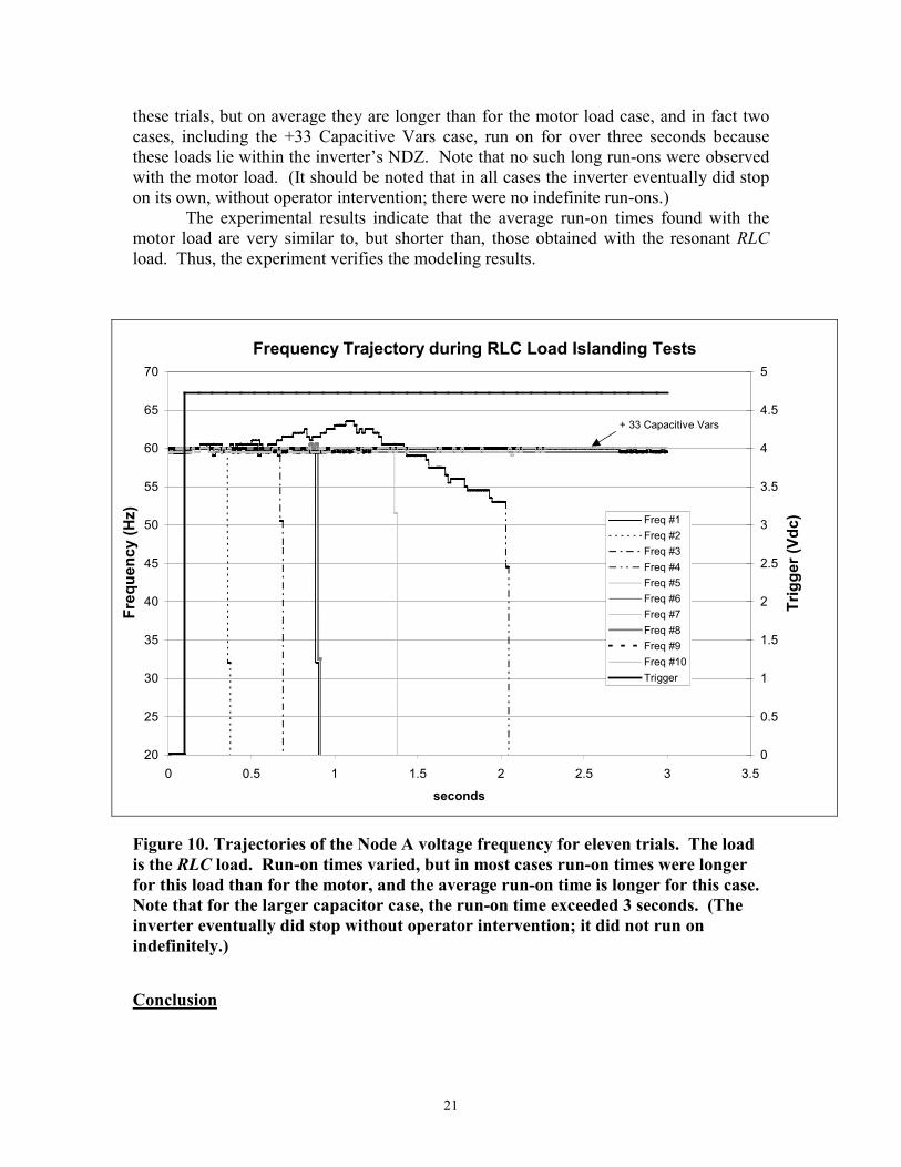
Figure 10 shows the results for the equivalent RLC load. Eleven trials areincluded here as well, ten with a unity power factor load and one with the slightly largercapacitor (again labeled "+33 Capacitive Vars"). The run-on times vary somewhat in

21

these trials, but on average they are longer than for the motor load case, and in fact twocases, including the +33 Capacitive Vars case, run on for over three seconds becausethese loads lie within the inverter’s NDZ. Note that no such long run-ons were observedwith the motor load. (It should be noted that in all cases the inverter eventually did stopon its own, without operator intervention; there were no indefinite run-ons.)

The experimental results indicate that the average run-on times found with themotor load are very similar to, but shorter than, those obtained with the resonant RLCload. Thus, the experiment verifies the modeling results.

Frequency Trajectory during RLC Load Islanding Tests

20

25

30

35

40

45

50

55

60

65

70

0 0.5 1 1.5 2 2.5 3 3.5

seconds

Freq

uenc

y (H

z)

0

0.5

1

1.5

2

2.5

3

3.5

4

4.5

5

Trig

ger (

Vdc)Freq #1Freq #2Freq #3Freq #4Freq #5Freq #6Freq #7Freq #8Freq #9Freq #10Trigger

+ 33 Capacitive Vars

Figure 10. Trajectories of the Node A voltage frequency for eleven trials. The loadis the RLC load. Run-on times varied, but in most cases run-on times were longerfor this load than for the motor, and the average run-on time is longer for this case.Note that for the larger capacitor case, the run-on time exceeded 3 seconds. (Theinverter eventually did stop without operator intervention; it did not run onindefinitely.)

Conclusion

22

Based on both the simulation and experimental results, it is possible to concludethat induction motors do not represent a worse case load than the previously describedworst-case RLC load (high Q, and a resonant frequency within the trip setpoints of theDG). In fact, induction machines can be thought of as implementing a special case ofthat worst-case RLC load. It can also be concluded that the Sandia inverter test using theparallel RLC load does adequately test that inverters will not island, even in the presenceof induction machines. It is not necessary to augment the test with induction machines.

Suggested future work

Two directions for future work are suggested by this study. First, it would beinstructive to repeat this analysis using a full transient electromagnetic model for thesingle-phase induction machine, to verify the appropriateness of the simplified modelused here. Second, this study did not consider three phase machines in detail, particularlysuch issues as phase and winding interactions and unbalanced conditions. A treatment ofthree phase machines would be a useful extension of this study.

References

[1] IEEE Standard IEEE-929, Recommended Practice for Utility Interface ofPhotovoltaic (PV) Systems, 1999.[2] J. Stevens, R. Bonn, J. Ginn, S. Gonzalez, and G. Kern, Development and Testingof an Approach to Anti-Islanding in Utility-Interconnected Photovoltaic Systems, SandiaNational Laboratories Report, SAND2000-1939, August 2000.[3] M. Ropp, Design Issues for Grid-Connected Photovoltaic Systems, PhDdissertation, Georgia Institute of Technology, Atlanta, GA, December 1998.[4] M. Ropp, M. Begovic, A. Rohatgi, "Prevention of islanding in grid-connectedphotovoltaic systems," Progress in Photovoltaics 7, 1999, p. 39-59.[5] G. Kern, "The physical origins of islanding in dispersed generation systems,"draft copy, Ascension Technologies, October 26 1997.[6] G. Kern, "Status Report #6, Sandia Anti-Islanding Investigation," contract reportto Sandia National Laboratories, May 27, 1998.[7] M. Sarma, Electric Machines, 2nd ed., pub. West Publishing Co. 1994.[8] M. Ropp, M. Begovic, A. Rohatgi, G. Kern, R. Bonn, S. Gonzalez, "Determiningthe relative effectiveness of islanding detection methods using phase criteria andnondetection zones," IEEE Transactions on Energy Conversion 15 (3), September 2000,p. 290-296.[9] Parameters of a standard 50-kVA 7620 V – 240 V transformer supplied byHoward Industries, Laurel, MS.[10] S. J. Chapman, Electric Machinery Fundamentals, 3rd ed., pub. WCB McGraw-Hill, 1998.[11] B. Amin, Induction Motors: Analysis and Torque Control, 2nd ed., pub. B. Amin2001.

23

24

Appendix A

Motor and RLC Load Parameters Used in this Work

The motor parameters used here were taken from page 330 of Reference 7. Theseparameters were found to be “typical” of single-phase induction machines, but it shouldbe noted that the possible values for these parameters vary widely for actual machines.

For the motor:

R1 = 10 �L1 = 33.16 mHLm = L1Lw = Lx = Ly = Lz = 0.5*Lm

R2 = 11.5 �

Motor speed before utility disconnection = 1710 rpm (179.1 rad/sec), corresponding to asteady-state slip of 5%

Cres = Ccomp = 96.325 �F

For the parallel RLC load:

R = 54.92 �L = 73.0 mH

26