Sanjeet_thesis__Final

UCGE Reports

Number 20247

Department of Geomatics Engineering

Comparison of Assisted GPS and High Sensitivity GPS in Weak Signal Conditions

(URL: http://www.geomatics.ucalgary.ca/research/publications/GradTheses.html)

by

Sanjeet Singh

October 2006

UNIVERSITY OF CALGARY

Comparison of Assisted GPS and High Sensitivity GPS in Weak Signal

Conditions

by

Sanjeet Singh

A THESIS

SUBMITTED TO THE FACULTY OF GRADUATE STUDIES

IN PARTIAL FULFILMENT OF THE REQUIREMENTS FOR THE

DEGREE OF MASTER OF SCIENCE

DEPARTMENT OF GEOMATICS ENGINEERING

CALGARY, ALBERTA

October, 2006

© Sanjeet Singh 2006

i

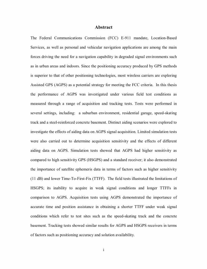
Abstract The Federal Communications Commission (FCC) E-911 mandate, Location-Based

Services, as well as personal and vehicular navigation applications are among the main

forces driving the need for a navigation capability in degraded signal environments such

as in urban areas and indoors. Since the positioning accuracy produced by GPS methods

is superior to that of other positioning technologies, most wireless carriers are exploring

Assisted GPS (AGPS) as a potential strategy for meeting the FCC criteria. In this thesis

the performance of AGPS was investigated under various field test conditions as

measured through a range of acquisition and tracking tests. Tests were performed in

several settings, including: a suburban environment, residential garage, speed-skating

track and a steel-reinforced concrete basement. Distinct aiding scenarios were explored to

investigate the effects of aiding data on AGPS signal acquisition. Limited simulation tests

were also carried out to determine acquisition sensitivity and the effects of different

aiding data on AGPS. Simulation tests showed that AGPS had higher sensitivity as

compared to high sensitivity GPS (HSGPS) and a standard receiver; it also demonstrated

the importance of satellite ephemeris data in terms of factors such as higher sensitivity

(11 dB) and lower Time-To-First-Fix (TTFF). The field tests illustrated the limitations of

HSGPS; its inability to acquire in weak signal conditions and longer TTFFs in

comparison to AGPS. Acquisition tests using AGPS demonstrated the importance of

accurate time and position assistance in obtaining a shorter TTFF under weak signal

conditions which refer to test sites such as the speed-skating track and the concrete

basement. Tracking tests showed similar results for AGPS and HSGPS receivers in terms

of factors such as positioning accuracy and solution availability.

ii

Acknowledgements

I would not be here if it not for the following people who have encouraged, supported

and provided motivation enabling me to complete my thesis. I would like to thank:

• Dr Elizabeth Cannon and Dr. Richard Klukas for their continued financial

support, encouragement and guidance which have been valuable and has enriched

my knowledge in the field of GPS.

• My parents in Lautoka Fiji, my Kaka, Kaki (uncle and aunt in Hindi) from Red

Deer AB, my cousins, Nikita, Krishen and Neelam, and my brother, Somjeet for

their love, care, moral and financial support.

• SiRF Technology Inc. (www.sirf.com) for proving us with the AGPS receiver. I

would like to thank Geoffery Cox and Lionel Garin (now at NemeriX) for

answering many questions. Finally Greg Turetzky at SiRF is also acknowledged.

• Gerard Lachepelle is also acknowledged for his encouragement throughout the

course of my program.

• Mr Ajay Varma, Binita Devi, Alvin, Amanda, Shyna for their moral support and

continued encouragement.

• Dharshaka Karunanayake for his continued loyalty, friendship and encouragement

throughout my research.

• Mr Merlin Keillor, Judy Smith and Pat Pardo from the Disability Resource Centre

at the University of Calgary for providing assistive devices and the 42’’ plasma

screen.

iii

• My friends and colleagues who were or are in the PLAN group; Anastasia

Salycheva, Chaminda Basnayike, Cecile, Bao Zhang, Gao, Glenn MacGougan,

Oleg , Olivier Jullien, Rob Watson, Sameet Deshpande, Salman Syed, Saurabh,

Seema Phalke, Shahin and Tao Hu, for their assistance and friendship

• My online friends either from www.indofiji.com or msn messenger for keeping

me company and sane when I was stressed; or during those long lonely nights;

Ranjit R. Raju, Shalini Chand (Miss Princess), Sanjana, Jotishna (Tishy), Agnes,

Sangeeta, Vandana¸ Uma (Sugalicious), Anuresh Chandra (Legend), Gine and

Urmila (Priya).

• Sean Mow and the staff at the Olympic Oval for giving us exclusive access to the

facilities to enable us to carry out numerous field tests.

• My soccer buddies of Nitin Nand, Rohit Kumar, Ravi Padurath and Rajnay Dayal.

• Mr Emmeron Glennon from Signav Navigation, Australia for his willingness to

help and give me much needed advice in the field of AGPS.

• Dr Paul McBurney from Eride Inc for a very nice presentation and advice in the

exciting field of AGPS

iv

Dedication

v

Table of Contents CHAPTER 1: INTRODUCTION..............................................................................1

1.1 Motivation ........................................................................................................2

1.2 Literature Review .............................................................................................3

1.3 Thesis Objectives..............................................................................................7

1.4 Thesis Overview ...............................................................................................8

CHAPTER 2: AGPS AND HSGPS THEORY ..........................................................9 2.1 GPS Signal Structure ........................................................................................9

2.1.1 GPS Measurement Error Sources.........................................................11

2.2 GPS Receiver Architecture .............................................................................13

2.2.1 GPS Signal Power and Signal to Noise Ratio (SNR)............................15

2.2.2 GPS Signal Acquisition.......................................................................17

2.2.2.1 Coherent Integration .............................................................21

2.2.2.2 Non-Coherent Integration .....................................................22

2.2.2.3 Comparison of Coherent and Non-Coherent Integration ........23

2.2.3 GPS Signal Tracking ...........................................................................24

2.2.3.1 Code Tracking Loop .............................................................25

2.2.3.2 Carrier Tracking Loop ..........................................................27

2.3 High Sensitivity GPS Challenges ....................................................................28

2.3.1 Multipath.............................................................................................29

2.3.2 Weak or Degraded GPS Signals ..........................................................30

2.3.3 HSGPS Implementations .....................................................................32

2.4 Assisted GPS (AGPS).....................................................................................34

2.4.1 Assistance Data –Wireless Networks...................................................35

vi

2.4.2 Almanac and Ephemeris Aiding ..........................................................37

2.4.3 Time and Approximate User Position Aiding ......................................38

2.4.4 Frequency Aiding................................................................................41

2.4.5 Interference Effects .............................................................................42

2.4.6 AGPS Implementation.........................................................................44

CHAPTER 3: SIMULATION TESTS.....................................................................47 3.1 Test Measures.................................................................................................47

3.2 Acquisition Tests ............................................................................................49

3.2.1 Test Objectives....................................................................................49

3.2.2 Test Methodology ...............................................................................50

3.2.3 Test Results and Analysis ....................................................................53

3.3 Chapter Summary ...........................................................................................61

CHAPTER 4: FIELD TESTS: ACQUISITION.......................................................62 4.1 Test Objectives ...............................................................................................62

4.2 Test Methodology...........................................................................................63

4.3 Field Test Environments .................................................................................66

4.3.1 Suburban Environment ........................................................................66

4.3.2 Residential Garage ..............................................................................68

4.3.3 Speed-Skating Track ...........................................................................70

4.3.4 Concrete Basement..............................................................................72

4.4 High Sensitivity GPS Receiver .......................................................................73

4.5 Timing Assistance ..........................................................................................75


4.5.2 Residential Garage ..............................................................................81

vii

4.5.3 Speed-skating Track ............................................................................86

4.5.4 Concrete Basement..............................................................................90

4.6 Horizontal Position Assistance........................................................................96


4.6.2 Residential Garage ............................................................................100

4.6.3 Speed-skating Track ..........................................................................102

4.6.4 Concrete Basement............................................................................105

4.7 Ephemeris and Almanac Assistance ..............................................................108

4.8 Comparison of Different Environments.........................................................111

4.9 Comparison of Simulation & Field Tests.......................................................117

4.10 Chapter Summary...........................................................................118

CHAPTER 5: FIELD TESTS: TRACKING..........................................................120 5.1 Test Objectives .............................................................................................120

5.2 Field Test Methodology ................................................................................120

5.3 Suburban Environment .................................................................................122

5.4 Residential Garage........................................................................................ 133

5.5 Speed-skating Track......................................................................................140

5.6 Concrete Basement Test................................................................................148

5.7 Comparison of Different Environments.........................................................154

5.8 Chapter Summary .........................................................................................157

CHAPTER 6: CONCLUSIONS & RECOMMENDATIONS................................159 6.1 Conclusions ..................................................................................................159

6.2 Recommendations.........................................................................................161

REFERENCES .......................................................................................................163

viii

List of Tables

Table 2.1: GPS Error Sources [Source: Lachapelle, 2002] .............................................13

Table 2.2: GPS Signal Power [Source: MacGougan, 2003]............................................16

Table 2.3: Message Structure for Point to Point Method [Source: LCS. 1999] ...............37

Table 2.4: Mobile Operating Frequencies [Source: Paddan et al., 2001] ........................43

Table 3.1: Acquisition Sensitivities of different SiRF Receivers ....................................54

Table 3.2: AGPS- Acquisition Sensitivities with different Test Scenarios......................54

Table 3.3: AGPS Position Results Using Least Squares.................................................60

Table 3.4: AGPS Position Results SiRF Internal Solution .........................................60

Table 4.1: Description of Different Aiding Scenarios ....................................................65

Table 4.2: HSGPS Receiver- Position Results Using LSQ Internal Solution for Roof and

Garage Tests..........................................................................................................74

Table 4.3: HSGPS Receiver- Position Results Using SiRF Internal Solution for Roof and

Garage Tests..........................................................................................................74

Table 4.4: Precise Time- Position Results Using LSQ for Suburban Test.......................76

Table 4.5: Precise Time Aiding - Position Results Using the SiRF Internal Solution

Suburban Test........................................................................................................77

Table 4.6: Coarse Time Aiding- Position Results Using LSQ for Suburban Test ...........78

Table 4.7: Coarse Time Aiding- Position Results Using SiRF Internal Solution for

Suburban Test........................................................................................................78

Table 4.8: Precise Time Aiding - Position Results Using LSQ for the Garage Test ........82

Table 4.9: Precise Time Aiding - Position Results Using SiRF Internal Solution for

Garage Test ...........................................................................................................82

ix

Table 4.10: Coarse Time Aiding - Position Results Using LSQ for Garage Test ...........83

Table 4.11: Coarse Time Aiding - Position Results Using SiRF Internal Solution for

Garage Test ...........................................................................................................84

Table 4.12: Precise Time - Aiding Position Results Using LSQ for Speed-skating Test .87

Table 4.13: Precise Time Aiding - Position Results using SiRF Internal Solution for

Speed-skating Test.................................................................................................88

Table 4.14: Precise Time Aiding - Position Results using LSQ Concrete Basement Test91

Table 4.15: Precise Time Aiding - Position Results using SiRF internal Solution for

Concrete Basement Test ........................................................................................91

Table 4.16: Coarse Time Aiding - Position Results Using LSQ for Concrete Basement

Test .......................................................................................................................92

Table 4.17: Coarse Time Aiding - Position Results using SiRF Internal Solution for

Concrete Basement Test ........................................................................................93

Table 4.18: Horizontal Position Aiding- Position Results using LSQ Solution for

Suburban test .........................................................................................................98

Table 4.19: Horizontal Position Aiding- Position Results for SiRF Internal Solution for

Suburban Test........................................................................................................99

Table 4.20: Horizontal Position Aiding- Position Results using LSQ Solution for Garage

Test .....................................................................................................................101


Garage Test .........................................................................................................101

Table 4.22: Horizontal Position Aiding- Position Results using LSQ Solution for Speed-

skating Test .........................................................................................................103

x


Speed-skating Test...............................................................................................104

Table 4.24: Horizontal Position Aiding– Position Results using LSQ Solution for

Concrete Basement ..............................................................................................106

Table 4.25: Horizontal Position Aiding– Position Results for SiRF Internal Solution for


Table 4.26: Ephemeris or Almanac Aiding- Position Results Aiding Using LSQ for all

the Test Sites .......................................................................................................109

Table 4.27: Ephemeris or Almanac Aiding - Position Results Using SiRF Internal

Solution for all the Test Sites ...............................................................................110

Table 4.28: Position Results Using LSQ Solution Under Different Field Test Conditions

............................................................................................................................114

Table 5.1: Dates of Tracking Field Tests .....................................................................122

Table 5.2: Horizontal Position Results using 67% and 95% of the Best Results for the

Three Receivers in the Suburban environment .....................................................132

Table 5.3: Azimuth/Elevation of Satellites in the Speed-skating Track ........................141

xi

List of Figures

Figure 2.1: GPS Signal Structure [Deshpande, 2004].....................................................10

Figure 2.2: GPS Receiver Architecture [ Source: MacGougan, 2003] ............................14

Figure 2.3: 2-D Acquisition Search Space .....................................................................20

Figure 2.4: Comparison of Coherent and Non-Coherent Integration [Source: Park et al.,

2004] .....................................................................................................................24

Figure 2.6: AGPS Concept ............................................................................................35

Figure 2.7: AGPS implementation [Source: Chiang, 2005]............................................46

Figure 3.1: Simulator Test Set-up ..................................................................................51

Figure 3.2: Simulator Set-up Schematic.........................................................................51

Figure 3.3: Comparison of AGPS test with Default Aiding, Hot start and without

Almanac Assistance...............................................................................................55

Figure 3.4: Comparison of AGPS Test with Warm Start and without Ephemeris

Assistance..............................................................................................................56

Figure 3.5: Comparison of AGPS with Cold start and HSGPS.......................................57

Figure 3.6: Comparison of Hot, Warm and Cold start performance of the AGPS Receiver

..............................................................................................................................58

Figure 3.7: Changing the Power of the Strong Satellite Channel (PRN 06) for AGPS ....59

Figure 4.1: Field Test Set-up for the AGPS Receiver.....................................................66

Figure 4.2: Receiver Setup for the Suburban Field Test .................................................67

Figure 4.3: Reference Antenna and the Surrounding Site ...............................................67

Figure 4.4: Surrounding Area for the Test Site...............................................................68

Figure 4.5: Test Setup for the Garage Test.....................................................................69

xii

Figure 4.6: Surrounding Area for the Garage Test .........................................................69

Figure 4.7: Outside View of the Speed-skating Track ....................................................70

Figure 4.8: Receiver Setup for the Speed-skating Track Test .........................................71

Figure 4.9: Inside the Speed-skating Track ....................................................................71

Figure 4.10: Receiver Setup for the Concrete Basement Test.........................................72

Figure 4.11: Surrounding Area for the Concrete Basement Test.....................................73

Figure 4.12: Precise Time Aiding - Normalized TTFF and Position Fixes for Suburban

Test .......................................................................................................................76

Figure 4.13: Coarse Time Aiding- Normalized TTFF and Position Fixes for Suburban

Test .......................................................................................................................77

Figure 4.14: C/N0 PDF for the Suburban Test ................................................................80

Figure 4.15: Precise Time Aiding – Normalized TTFF and Position Fixes for Garage Test

..............................................................................................................................81

Figure 4.16: Coarse Time Aiding – Normalized TTFF and Position Fixes for Garage Test

..............................................................................................................................83

Figure 4.17: C/N0 PDF for the Residential Garage Test..................................................86

Figure 4.18: Precise Time Aiding – Normalized TTFF and Position Fixes for Speed-

skating Test ...........................................................................................................87

Figure 4.19: C/N0 PDF for the Speed-skating Track Test...............................................89

Figure 4.20: Precise Time Aiding – Normalized TTFF and Position Fixes for Concrete

Basement Test .......................................................................................................90

Figure 4.21: Coarse Time Aiding – Normalized TTFF and Position Fixes for Concrete

Basement Test .......................................................................................................92

xiii

Figure 4.22: C/N0 PDF for the Concrete Basement Test .................................................95

Figure 4.23: Time Relationship for L1 C/A Code [Source: Kaplan and Hegarty, 2006]..96

Figure 4.24: Horizontal Position Aiding- Normalized TTFF and Position Fix for

Suburban test .........................................................................................................98

Figure 4.25: Horizontal Position Aiding- Normalized TTFF and Position Fix for Garage

Test .....................................................................................................................100

Figure 4.26: Horizontal Position Aiding – Normalized TTFF and Position Fix for Speed-

skating Test .........................................................................................................103

Figure 4.27: Horizontal Position Aiding – Normalized TTFF and Position Fix for


Figure 4.28: Precise Time Aiding- Normalized TTFF and Number of Satellites Tracked

for Different Test Sites ........................................................................................112

Figure 4.29: Horizontal Position Aiding- Normalized TTFF and Number of Satellites for

Different Test Sites..............................................................................................113

Figure 4.30: Horizontal Error and the Number of Satellites Tracked for Residential

Garage Test .........................................................................................................116

Figure 4.31: Horizontal Error and the Number of Satellites Tracked for Concrete

Basement Test .....................................................................................................117

Figure 5.1: Field Set-up for Tracking Tests..................................................................121

Figure 5.2: Azimuth and Elevation for the Satellites Tracked in the Suburban Test......123

Figure 5.3: AGPS Receiver Position Results for the Suburban Test .............................124

Figure 5.4: HSGPS Receiver Position Results for the Suburban Test ...........................125

Figure 5.5: Standard Receiver Position Results for the Suburban Test .........................126

xiv

Figure 5.6: Time Series for the C/N0 for AGPS Receiver for the Suburban Test ..........127

Figure 5.7: Time Series of Residual Errors for the AGPS Receiver the Suburban Test.127

Figure 5.8: Time Series for the C/N0 for HSGPS Receiver the Suburban Test.............128

Figure 5.9: Time Series of Residual Errors for the HSGPS Receiver for the Suburban

Test .....................................................................................................................128

Figure 5.10: Time Series for the C/N0 for Standard Receiver for the Suburban Test.....129

Figure 5.11: Time Series of Residual Errors for the Standard Receiver for the Suburban

Test .....................................................................................................................129

Figure 5.12: Azimuth/Elevation Profile of Average C/N0 for the Suburban Test ..........130

Figure 5.13: Azimuth and Elevation for the Satellites in the Residential Garage Test...134

Figure 5.14: AGPS Receiver Position Results for the Residential Garage Test............135

Figure 5.15: HSGPS Receiver Position Results for the Residential Garage Test ..........136

Figure 5.16: Time Series for the C/N0 for AGPS Receiver for the Residential Garage Test

............................................................................................................................137

Figure 5.17: Time Series of Residual Errors for the AGPS Receiver for the Residential

Garage Test .........................................................................................................137

Figure 5.18: Azimuth/Elevation Profile of Average C/N0 for the Garage Test..............138

Figure 5.19: AGPS Receiver Position Results for the Speed-skating Track..................142

Figure 5.20: HSGPS Receiver Position Results for the Speed-skating Track................143

Figure 5.21: Time Series for the C/N0 for AGPS Receiver for the Speed-skating Track144

Figure 5.22: Time Series of Residual Errors for the AGPS Receiver for the Speed-skating

Track ...................................................................................................................145

Figure 5.23: Azimuth/Elevation Profile of Average C/N0 for the Speed-skating Test ...146

xv

Figure 5.24: Azimuth Elevation for the Satellites in the Concrete Basement Test ........148

Figure 5.25: AGPS Receiver Position Results for the Concrete Basement Test ............149

Figure 5.26: HSGPS Receiver Position Results for the Concrete Basement Test..........150

Figure 5.27: Time Series for the C/N0 for AGPS Receiver for the Concrete Basement

Test .....................................................................................................................151

Figure 5.28: Time Series of Residual Errors for the AGPS Receiver for the Concrete

Basement Test .....................................................................................................151

Figure 5.29: Azimuth/Elevation Profile of Average C/N0 for the Concrete Basement Test

............................................................................................................................152

Figure 5.30: Position Solution for Suburban Test using the AGPS Receiver ................154

Figure 5.31: Position Solution for Residential Garage Test using the AGPS Receiver..155

Figure 5.32: Position Solution for Speed-skating Track Test using the AGPS Receiver155

Figure 5.33: Position Solution for Concrete Basement Test using the AGPS Receiver .156

xvi

List of Abbreviations

Abbreviations and Acronyms

A/D Analog-to-Digital AFC Automatic Frequency Control AGC Automatic Gain Control AGPS Assisted GPS AM Amplitude Modulation AoD Age of Data ASIC Application Specific Integrated Circuit BiCMOS Bipolar Complementary Metal Oxide

semiconductor C/A Coarse/Acquisition CCIT Calgary Centre for Innovative Technologies CDMA Code Division Multiple Access C/N0 Carrier to Noise Ratio CTL Carrier Tracking Loop C/W Continues Wave DGPS Differential GPS DFT Discrete Fourier Transform DLL Delay Lock Loop DOP Dilution of Precision DSP Digital Signal Processing E-911 Enhanced 911 E-OTD Enhanced Observed Time Difference FCC Federal Communications Commission FFT Fast Fourier Transform FLL Frequency Lock Loop FM Frequency Modulation GPS Global Positioning System GNSS Global Navigation Satellite System GSM Global System for Mobile Communications HDOP Horizontal DOP

HSGPS High Sensitivity GPS I In-phase IE Information Element IM Instant Messaging ION Institute of Navigation LBS Location Based Services LMU Location Measurement Unit LNA Low Noise Amplifier LOS Line of Sight

xvii

LSQ Least Squares MEDLL Multipath Estimation Delay Lock Loop MET Multipath Elimination Technique NCO Numerical Controlled Oscillator NLOS Non-Line of Sight PLAN Position Location and Navigation PLL Phase Lock Loop PRN Pseudorandom PVT Position Velocity Time Q Quadrature- phase RF Radio Frequency RFI Radio Frequency Interference SNR Signal to Noise Ratio SoC Silicon on Chip TEC Total Electron Content TOA Time Of Arrival TTB Time Transfer Board TTFF Time To First Fix

1

CHAPTER 1: INTRODUCTION

The US Federal Communication Commission (FCC) has set regulations (Phase I and Phase

II) for accurate cellular positioning, i.e. Enhanced E-911 [FCC, 2001]. There has also been

an increase in the demand for Location-Based Services (LBS). These services would

include mobile applications such as personal navigation using digital maps. These two

applications have been pushing for accurate positioning solutions. The Global Positioning

System (GPS) has so far proven to be a more accurate positioning solution when compared

with existing cellular positioning technologies. GPS can give the end user an accuracy of

within 30 m, unlike cellular positioning techniques such as Enhanced Observed Time

Difference (E-OTD) which can deliver accuracies in the range of over 100 m [Syrjärinne,

2001]. However, just like any satellite-based technology, GPS suffers from signal

obscuration or blockage in urban or indoor environments which would reduce satellite

availability and multipath effects from materials such as wood concrete or glass would

degrade the positioning accuracy. Furthermore, shadowing or signal attenuation produce

weak signal conditions (< -150 dBm) which tend to make it difficult or impossible to

acquire or effectively track GPS signals. A conventional receiver’s inability to acquire or

track GPS signals under weak or degraded signal conditions has prompted the development

of High Sensitivity GPS (HSGPS) and Assisted GPS (AGPS) technologies. AGPS and

HSGPS carry out longer coherent and non-coherent integration enabling them to acquire

and or track weaker GPS signals (-160 dBm).

2

The Position Location and Navigation (PLAN) Group of the Schulich School of

Engineering, University of Calgary has been active in assessing the performance of HSGPS

receivers in degraded signal environments using field and Radio Frequency (RF) simulation

experiments [MacGougan, 2003]. In indoor environments, with the availability of AGPS, it

is now possible to directly acquire signals in weak signal environments using assistance

data from a network server or a reference receiver [van Diggelen, 2001]. Recently, various

simulation tests have been carried out using an RF simulator to determine the effects of

various aiding parameters on the acquisition performance of the AGPS receiver

[Karunanayake, 2005b]; however, further research is required to investigate effects of

different types of aiding data under various field signal conditions. Tracking tests were

carried out to illustrate the similarities between AGPS and HSGPS receivers. While

simulation tests provide results based on a limited range of controlled environments, the

variety of actual end-user signal reception situations requires a wider array of field test sites

that would more realistically indicate actual and distinct challenges to the AGPS receiver in

terms of the factors discussed above, based on different aiding scenarios.

1.1 Motivation

The requirement set out by the FCC-E911 phase II mandate requires cell phone service

providers to locate mobile users with an accuracy of 50 m for 67 % of the time, and with an

accuracy of 150 m for 95 % of the time for handset based technologies [FCC, 2001]. There

has been a steady increase in the demand for LBS due to the rise in the number and variety

of mobile devices which has led to many exciting applications. Some LBS applications

include mobile-gaming; vehicular or personal navigation; locating restaurants or hotels

3

within a specified range; coordinating the location of groups of friends; and chatting

services similar to traditional Instant Messaging (IM) applications such as Yahoo TM and

MSNTM Messenger. Across this potential range, factors such as quality of service, limited

storage capacity or battery power supply require positioning technologies such as AGPS or

HSGPS to implement power-saving implantation strategies and faster signal acquisition

schemes for more rapid position fixing. The various LBS application and E-911 mandate

requires cell phones to work in many different signal conditions which was major driving

force for conducting this research. HSGPS and AGPS receivers were tested in particularly

weak signal conditions, where conventional receivers are unable to acquire or track signals.

1.2 Literature Review

Field and simulation tests have been carried out using the SiRF StarII HSGPS and SiRF

standard receivers to demonstrate the effects of longer integration time [Shewfelt et al.,

2001]. The HSGPS receiver carried out a coherent integration for 1 ms followed by non-

coherent integration episodes of 4 ms, 12 ms and 16 ms durations, and was able to detect

GPS signal strengths with carrier to noise ratio (C/N0) levels of 39 dB-Hz, 35 dB-Hz and 30

dB-Hz, respectively. Simulation tests in a weak signal environment (30 to 35 dB-Hz) have

shown that the HSGPS receiver had a shorter Time-To-First-Fix (TTFF), as compared to a

standard receiver, while field tests that were carried out in a San Francisco road tunnel

established that the HSGPS receiver had better solution availability compared to a standard

receiver.

4

To compare the tracking performance of HSGPS (SiRF StarII) and conventional (NovAtel

OEM4 and SiRF standard) GPS receivers under different weak/degraded signal conditions,

field and simulation tests were carried out by the University Calgary’s PLAN Group

[MacGougan et al., 2002]. Static field tests were also carried out in a residential wood and

concrete garage. The results of the various tests demonstrated the ability of an HSGPS

receiver to give position fixes in an indoor environment; the HSGPS receiver was able to

deliver a position with an accuracy of 50 m (RMS), while a conventional receiver was

unable to provide a position fix indoors. The HSGPS also performed better in terms of

positioning accuracy and availability under weak or degraded signal conditions. Simulation

tests also demonstrated the HSGPS receiver’s superior acquisition sensitivity (10 dB) in

comparison to conventional GPS receivers.

Field tests have been carried out by SiRF Technology Inc. using the SiRFLocTM client

AGPS receiver under various field test situations [Garin et al., 1999]. Test conditions used

were a parking lot, a narrow walkway between tall buildings, a shopping mall with a glass

roof, and inside a two-storey building close to a window. Results indicate that the AGPS

receiver was able to obtain a position fix with an accuracy of 100 m under most of these

field test conditions; the exception, however, was the achievement of a positioning accuracy

of only 184 m for the narrow walkway due to poor satellite availability. Further simulation

tests have been performed to determine the effects of different power levels, specifically in

terms of the TTFF and positioning accuracy [Garin et al., 2002]. The simulation tests

revealed longer TTFFs and degraded horizontal positioning accuracy levels, with

5

decreasing power levels for the AGPS receiver. The SiRFLocTM is a multimode receiver,

which can operate in either an assisted or standalone HSGPS mode.

Field tests were conducted by Moeglein and Krasner [1998] with the aid of SnapTrackTM (a

product that was later acquired by Qualcomm Inc.) in an outdoor, urban environment,

inside a sport utility vehicle located in a concrete parking garage, as well as in the basement

of a two-storey building; in a two-storey office building in the urban centre of Denver, CO;

and on the 21st floor of a 50-storey glass building, also in Denver. Test results demonstrate

a positioning accuracy, in most cases, of within 30 m, a figure that was progressively

degraded with increasing hostility of the testing conditions. The worst results were obtained

in the setting of the 50-storey glass-clad office building (84 m for 68.3 % of the best

results); the yield or percentage of successful position fixes also decreased, with the

receiver delivering a yield of 89% for the 50-storey test.

Data obtained from the deployment of Qualcomm’s gpsOneTM solution, which employs a

hybrid methodology of AGPS (functioning in the mobile-assisted mode) and cellular

positioning technologies, showed that AGPS was used for 84% of the time to obtain a

position solution, where the test sites ranged from subways to urban canyon environments,

characterised by low satellite availability and highly attenuated GPS signals [Biacs et al.,

2002]. The hybrid cellular and AGPS solution can be used to increase the solution

availability, employing either the AGPS or cellular individually or in conjunction, to obtain

the position solution.

6

Field tests have been conducted by van Diggelen and Abraham [2001] using Global

Locate’s GL-16000TM AGPS receiver under various field test conditions such as downtown

San Francisco; inside a shirt pocket; in the cab of a steel truck traveling at 112 km/h; within

a four-story building; and inside a shopping mall. The maximum TTFF in these trials was

obtained at the bottom floor of a four-storey building. Field tests were also carried out in a

concrete garage; downtown San Francisco; in a two-storey office building; and within a

drawer inside the two-storey office building. Results showed a mean accuracy of within 25

m. The GL-16000TM chipset is a multimode receiver, which uses 16000 hardware

correlators, where the aiding data was provided from their worldwide reference network.

Sigtech Navigation’s subATTOTM technology demonstrated an acquisition sensitivity of -

155 dBm [Bryant et al., 2001]. The receivers were assisted by satellite ephemeris and

almanac data, as well as approximate time and position, to hasten the acquisition process.

The field tests were carried out in a parking garage on the uppermost level of a three-storey

building; and two floors below the top. A signal strength of less than 30 dB-Hz was

observed at two floors below the top, with a positioning accuracy of within 50 m.

Numerous simulation tests have been carried out under static conditions to explore the

effects of various aiding parameters on GPS receivers [Karunanayake et al., 2004]. Such

tests confirm the importance of accurate time or position aiding under weak signal

conditions (-140 dBm), while tracking tests have shown that AGPS and HSGPS had the

same tracking threshold which was 15 dB better than that of conventional receivers.

7

1.3 Thesis Objectives

There are no documented attempts within the existing literature detailed above to compare

the tracking performance of HSGPS and AGPS receivers, or to determine the effects of

different types of aiding data on AGPS signal acquisition under various field test

conditions. To address this gap in the literature, the following thesis objectives are

proposed:

1) Compare the acquisition performance of AGPS under different aiding scenarios

using the hardware simulator;

2) Investigate the effects of variations in timing uncertainty on AGPS signal

acquisition at different field test sites;

3) Determine the effects of varying the horizontal position uncertainty on AGPS signal


4) Determine the effects of satellite ephemeris or almanac aiding on AGPS signal


5) Compare acquisition performance of an AGPS receiver under different field test

conditions; and

6) Investigate the tracking performance of HSGPS and AGPS receivers under different

field test conditions.

8

1.4 Thesis Overview

Chapter 2 provides the theoretical background of concepts such as the GPS signal structure;

receiver architecture; signal power; signal acquisition or tracking schemes; along with

HSGPS and AGPS implementation details. Chapter 3 presents a discussion of simulation

tests conducted to determine the effects of various types of aiding data on AGPS acquisition

sensitivity. Chapter 4 discusses acquisition tests carried out under various field conditions

and aiding scenarios, while Chapter 5 presents the results and analysis from tracking tests

carried out in distinct field test conditions using HSGPS and AGPS receivers. Finally,

Chapter 6 presents conclusions and recommendations for future work.

9

CHAPTER 2: AGPS AND HSGPS THEORY

This chapter provides the theoretical background on AGPS and HSGPS. Section 2.1

discusses the basics of the GPS signal structure, measurement attributes, and possible

measurement error sources. Section 2.2 then gives a discussion of aspects of the receiver

architecture including thermal noise, acquisition schemes, and possible ways of integrating

tracking loops through the use of code or carrier tracking loops. In Section 2.3, a discussion

of HSGPS challenges and possible implementation schemes is given, followed by a

discussion of AGPS concepts and implementation strategies currently employed by certain

companies in production model receivers.

2.1 GPS Signal Structure

GPS is a satellite-based positioning system capable of providing a user position anywhere

in the world. This system was developed by the U.S. Department of Defense (DoD) to

support the military forces of the United States of America by delivering world-wide, real-

time positions [Parkinson et al., 1995]. GPS can be used for civilian applications even

though it was originally developed for military applications [Spilker and Parkinson, 1996].

The system currently consists of a constellation of 27 (nominally 24) satellites and an

associated network of ground stations, which transmit, through the satellites, continuous

information for the user to compute position, velocity and time (PVT).

GPS transmits on two carrier frequencies referred to as L1 (1575.42 MHz, the primary

frequency) and L2 (1226.7 MHZ, the secondary frequency) as illustrated in Figure 2.1.

10

These two frequencies are modulated by a pseudorandom noise (PRN) code, which is in

turn modulated by the 50 Hz navigation data message. Two spreading codes are used to

modulate these carriers. The precision P(Y) code is present on both L1 and L2, and has a

chipping rate of 10.23 MHz which repeats after a period of 38 weeks.

Figure 2.1: GPS Signal Structure [Deshpande, 2004]

Range can be measured by differencing the time of transmission from the time of reception

for the GPS signals; however, since the clocks contained in the GPS satellite and the

receiver are not synchronized, the measured range is characterised at this point as a

pseudorange [Kaplan and Hegarty, 2006]. Civilian GPS receivers rely on L1

Coarse/Acquisition (C/A) code measurements, which are modulated on the L1 carrier. The

C/A code is replicated in the GPS receiver and can be correlated with the incoming signal

to output pseudorange information. Pseudorange measurements from four or more satellites

are required to compute three unknowns in the position domain (x, y and z) and the receiver

clock bias.

11

The relative velocity between the transmitter and receiver results is a physical phenomenon

known as a Doppler shift [Tsui, 2000]. Doppler would cause a change in the frequency that

is observed by the receiver due to the relative motion between a receiver and transmitter - in

this case the GPS satellite. An analysis of the Doppler effect can be used to compute the

user’s velocity. At least four measurements are required to compute three velocity

components (vx, vy and vz) and the receiver clock drift. The maximum Doppler shift would

be 5 kHz for a static user, and reaching up to 10 kHz for a high-speed flying aircraft.

2.1.1 GPS Measurement Error Sources

A GPS measurement is corrupted by errors such as control segment errors; furthermore,

satellite clock or ephemeris errors, and uncertainties in the propagation medium may affect

the signal’s travel time from the satellite to the receiver [Misra and Enge, 2001]. These

errors can be categorised into either ionospheric or tropospheric delay components. Noise

observed at the receiver is typically caused by interference from surrounding sources.

Reflected or multipath signals, also affect the accuracy of the measurement.

The ephemeris and satellite clock parameter values broadcast by the satellite are computed

by the control segment with the use of measurements from the GPS monitoring stations.

There are errors associated with the prediction of the current and/or future values of the

parameters; the prediction errors grow with the Age-of-Data (AoD), which is defined

relative to the time when the parameters were last uploaded. Satellite clock error is due to

satellite clock drift with respect to the GPS time reference.

12

The ionosphere is a region consisting of ionized gas (free electrons and ions) that extends

from 50 km to 1000 km above the Earth. The ionization is the result of solar radiation; the

speed of propagation of the GPS signal depends on the number and density of free

electrons, which is referred to as the Total Electron Content (TEC). The TEC may vary,

depending on such factors as solar radiation or geometric distance and is at least one or two

orders of magnitude greater during the day than at night. The ionosphere is dispersive; that

is, because the velocity is dependent on frequency, ionospheric errors can be eliminated

with the use of dual frequency L1/L2 GPS receivers.

The troposphere describes an oblate region consisting of water vapour (found below an

altitude of 12 km), and dry gas which can be found 16 km above the equator and 9 km

above the poles. The components of the tropospheric error which result from dry gas or

water vapour are known as dry and wet delays, respectively. The troposphere is non-

dispersive and, thus, its effects cannot be isolated by dual frequency measurements.

Receiver noise is caused by factors such as amplifiers, cables and interference from other

sources such as wireless networks or GPS-like broadcast sources which may be augmented

with the GPS receiver. Multipath is another source of measurement error, where the Line of

Sight (LOS) signal may combine with various reflected components as affected by various

reflective surfaces along the path. A further discussion of multipath is provided in Section

2.3.1. Table 2.1 shows the 1σ values for a range of GPS error sources.

13

Table 2.1: GPS Error Sources [Source: Lachapelle, 2002]

GPS Error Source Error Magnitude (1σ)

(m)

Satellite clock and orbital errors 2.3

Ionosphere on L1 7.0

Troposphere 0.2 Code multipath 0.01-10

Code noise 0.6

Carrier multipath 50x10-3

Carrier noise 0.2-2x10-3

2.2 GPS Receiver Architecture

As illustrated in Figure 2.2, GPS signals are received at the Radio Frequency (RF) front end

via a GPS antenna. After performing a series of pre-amplifications, band-pass filtering and

down-conversion steps on the GPS signals are conducted to transform them into

Intermediate Frequencies (IF) at the RF front end, before the signal is converted into

digitized samples using a Analogue to Digital (A/D) converter. The amplification is carried

out to set the noise floor, and band-pass filtering is carried out to reject noise, continuous

wave (CW) interference or jamming. Meanwhile, the signal is down-converted to enable

digitization because signal processing is easier to implement at much lower frequencies

than at the L1 frequency. During signal acquisition, the received signal is correlated with

the replica signal that is generated by the GPS receiver, to obtain coarse estimates of the

14

C/A code phase and satellite Doppler. After acquisition of the signal, the satellite can be

tracked with the use of tracking loops such as a DLL (code phase), PLL (phase lock loop)

or FLL (frequency lock loop). The navigation data bits are demodulated and pseudorange,

carrier phase or Doppler measurements obtained from the tracking loops for each satellite

are used to compute the user PVT. The following sub-sections provide a detailed

explanation of a typical GPS receiver architecture including the received signal power,

acquisition and tracking processes.

Figure 2.2: GPS Receiver Architecture [ Source: MacGougan, 2003]

15

2.2.1 GPS Signal Power and Signal to Noise Ratio (SNR)

A GPS satellite transmits approximately 27 W of power for the L1 C/A code, which is

equivalent to 10log10(27/10-3) yielding 44.3 dBm [Misra and Enge, 2001]. The signal

encounters free-space path loss that is dependent on the radius from the satellite to the

receiver; the transmitted power is increased by redirecting the signal towards the centre and

edge of the Earth rather than in all directions, whereby the direction is given by the nadir

angle α over the range ± 13.9°. Another important factor is the satellite’s elevation angle; a

satellite at low elevation has a higher gain of 12.1 dB, while satellites at the zenith provide

a gain of 10.2 dB. The gain is determined using the satellite’s antenna gain pattern. The

properties of the GPS antenna used to capture the signal affect the nature of the received

signal; its surface area determines the effective power captured while the gain pattern

focuses signal power in certain directions. The user antenna can receive signals only from

above the horizon, where the gain is invariant with azimuth; however, the gain does vary

with elevation, the particulars of which are captured using the antenna’s elevation pattern.

There are some antennas that reject interference or multipath from certain directions (from

other wireless emitters of GPS-like signals or nearby reflective sources) and can be

modeled with the use of the antenna’s gain pattern.

Techniques to alleviate the effects of multipath include Rays [2000] study of a multiple

antenna array in mitigating carrier phase multipath; and the use of a microstrip antenna

array to mitigate interference or jamming [Lin et al., 2002]. The GPS receiver employed in

this research uses a microstrip antenna which can either be embedded within the receiver or

16

connected separately; the advantages of this type of antenna include its small size and low

cost.

In comparison to other spread-spectrum communications signals, a GPS signal is very

weak, as shown in Table 2.2; however, other signals such as thermal noise generated by the

receiver or sources outside the receiver are also weak. For purposes of this study, thermal

noise can be modeled as white noise, in which case every frequency component is assumed

to have the same power; the power level of this noise is given by 2.1.

2.1

where:

K is Boltzman’s constant (1.38066e-23 J/K)

T is the Noise temperature (nominally 273°K), and

B is the nominal Bandwidth of noise.

Table 2.2: GPS Signal Power [Source: MacGougan, 2003]

SV Antenna Power (dBW) 13.4 S V Antenna Gain (dBW) 13.4

User Antenna Gain (hemispherical) (dB)

3.0

Free Loss L1 for R = 25092 km (dB) -184.4

Atmospheric Attenuation, (dB) -2.0 Depolarization Loss (dB) -3.4

User Received Power (dBW) -160 or -130 dBm

KTBNpower =

17

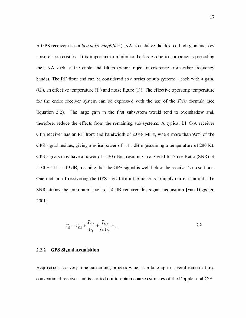
A GPS receiver uses a low noise amplifier (LNA) to achieve the desired high gain and low

noise characteristics. It is important to minimize the losses due to components preceding

the LNA such as the cable and filters (which reject interference from other frequency

bands). The RF front end can be considered as a series of sub-systems - each with a gain,

(Gi), an effective temperature (Ti) and noise figure (Fi), The effective operating temperature

for the entire receiver system can be expressed with the use of the Friis formula (see

Equation 2.2). The large gain in the first subsystem would tend to overshadow and,

therefore, reduce the effects from the remaining sub-systems. A typical L1 C/A receiver

GPS receiver has an RF front end bandwidth of 2.048 MHz, where more than 90% of the

GPS signal resides, giving a noise power of -111 dBm (assuming a temperature of 280 K).

GPS signals may have a power of –130 dBm, resulting in a Signal-to-Noise Ratio (SNR) of

-130 + 111 = -19 dB, meaning that the GPS signal is well below the receiver’s noise floor.

One method of recovering the GPS signal from the noise is to apply correlation until the

SNR attains the minimum level of 14 dB required for signal acquisition [van Diggelen

2001].

2.2

2.2.2 GPS Signal Acquisition

Acquisition is a very time-consuming process which can take up to several minutes for a

conventional receiver and is carried out to obtain coarse estimates of the Doppler and C/A-

...21

3,

1

2,1, +++=

GGT

GT

TT EEER

18

code phase before tracking can commence [Misra and Enge, 2001]. The receiver-generated

code is correlated with the incoming code and compared to the acquisition threshold to

determine if a useful signal is present. Signal detection is a statistical process; the C/A-code

phase or Doppler search bin (described below) may contain either a useful signal or noise;

the noise would have a zero mean characterised by a Rayleigh distribution, while a signal

with noise has a non-zero mean with a Rician distribution [Kaplan and Hegarty, 2006].

Signal detection is a binary process involving the noise and signal Probability Distribution

Function (PDF) in which a useful signal is detected by using parameters such as Pfd

(probability of detection) and Pfa (probability of false alarm). The Pfd should be chosen in

such a way as to enable signal detection, while Pfa must be chosen so as to ensure that noise

is not detected as a useful signal. If the receiver does not have a priori knowledge of the

approximate location, current GPS time or ephemeris, achieving a position fix could take

up to several minutes; without initial values for these data, a complete sky search of all

PRN codes, all Doppler and code phase bins is carried out and the navigation data needs to

be downloaded, each of which could take up to thirty seconds. AGPS receivers (see Section

2.4) rely on aiding data to shorten the acquisition search time. Once the receiver is provided

with assistance data such as approximate user position, current GPS time, and satellite

ephemeris or almanac, the acquisition search time can be reduced to a few seconds. The

receiver can use either hardware or software implementation schemes for signal acquisition

[Deshpande, 2003].

The hardware approach is implemented using Application-Specific Integrated Circuits

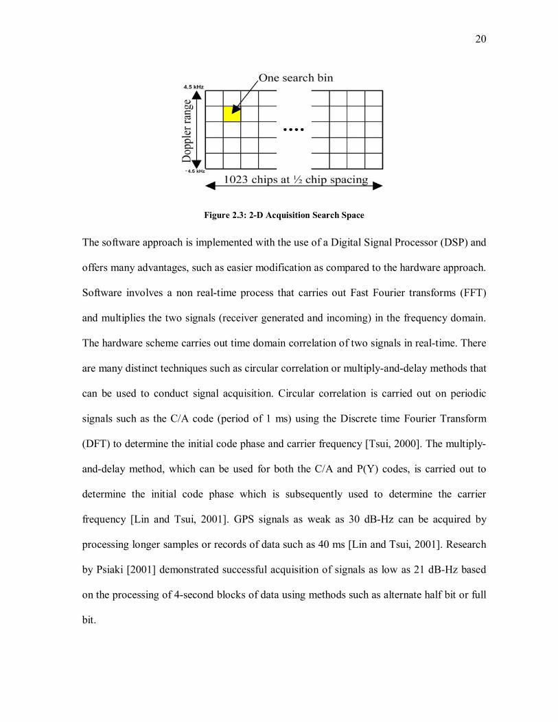
(ASIC) on a chipset. There are two unknowns and the search can be divided into a 2-D

19

search space of Doppler/C/A-code phase as illustrated in Figure 2.3 [Kaplan and Hegarty,

2006]. The 2-D frequency/ C/A-code search space could have a Doppler of ± 4.5 kHz and a

0-1022 chip C/A code phase. Correlation is performed in each cell by using the pre-

detection integration and comparing the correlation value with the detection threshold. If

the value is less than the threshold, the search goes onto the next cell until a useful signal is

found. Two samples per chip are used while searching for the correlation peak in the code

space; i.e. there are 2046 samples and, since there are two channels/satellite (In-phase (I)

and Quadrature-phase (Q)), there is a total of 4092 samples. The frequency width (fc) of the

bins is calculated by using Equation 2.3. As a rule of thumb, fc is 667 Hz for 1 ms and fc is

33 Hz for 20 ms. In order to search for one satellite with a 20 ms integration, there are

4092*(4500 + 4500)/67 bins (given by Equation 2.4), which results in 549672 bins,

suggesting that a longer integration time (required to detect weaker signals) results in a

longer search time or TTFF.

2.3

where fc is the frequency width of the bins and N is the integration time

2.4

where TB is the total number of bins, and fc is the frequency width of the bin.

Nfc 3

2=

fcTB /)45004500(*4092 +=

20

Figure 2.3: 2-D Acquisition Search Space

The software approach is implemented with the use of a Digital Signal Processor (DSP) and

offers many advantages, such as easier modification as compared to the hardware approach.

Software involves a non real-time process that carries out Fast Fourier transforms (FFT)

and multiplies the two signals (receiver generated and incoming) in the frequency domain.

The hardware scheme carries out time domain correlation of two signals in real-time. There

are many distinct techniques such as circular correlation or multiply-and-delay methods that

can be used to conduct signal acquisition. Circular correlation is carried out on periodic

signals such as the C/A code (period of 1 ms) using the Discrete time Fourier Transform

(DFT) to determine the initial code phase and carrier frequency [Tsui, 2000]. The multiply-

and-delay method, which can be used for both the C/A and P(Y) codes, is carried out to

determine the initial code phase which is subsequently used to determine the carrier

frequency [Lin and Tsui, 2001]. GPS signals as weak as 30 dB-Hz can be acquired by

processing longer samples or records of data such as 40 ms [Lin and Tsui, 2001]. Research

by Psiaki [2001] demonstrated successful acquisition of signals as low as 21 dB-Hz based

on the processing of 4-second blocks of data using methods such as alternate half bit or full

bit.

21

2.2.2.1 Coherent Integration

The L1 C/A code has a length of one millisecond and, so, coherent integration would

require successful correlation of at least one millisecond of incoming signal with the locally

generated replica. Coherent integration involves a summation of the In-phase components.

It is a band-pass process, in which each frequency bin represents a filter and the bandwidth

is inversely proportional to the integration time; a longer integration time would filter out

more noise and, hence, result in higher sensitivity [Zhengedi, 2000]. When conducting

coherent integration, signal power increases by N while the noise power increases by N

resulting in a SNR gain of N . A longer period of coherent integration results in finer

frequency resolution (see 2.3); hence, a larger processing gain can be realized,

achieving higher sensitivity at the expense of a longer search time [van Diggelen, 2001].

The 50 Hz navigation data is modulated with the C/A code imposing a limit of 20 ms on

coherent integration. The In-phase component incurs a sign inversion when it undergoes a

navigation data bit transition. Zhengedi [2000] has successfully achieved optimal gain

levels based on 10 ms of coherent integration. Longer integration times resulted in greater

loss as the probability of crossing the navigation bit boundary is increased, thus producing

errors that result in acquisition loss. Further research has shown the issue of longer

integration times, for example coherent accumulation over 20 ms resulted in a loss of 24 dB

using signal of 40 dB-Hz [Dafesh and Fan, 2001]. The loss was lower for weaker signals

since the thermal noise became a relatively more significant error source - for example,

where there was a loss of 3 dB with a signal strength of 20 dB-Hz. The signal losses were

22

lower for smaller integration times; that is, an integration time of 10 ms led to a loss of 16

dB for 40 dB-Hz signals. Longer integration is possible after bit prediction; a gain of 6 dB

was achieved when signals were integrated for 20 ms as compared to a 1 ms integration

period. Longer coherent integration is further limited because of residual frequency errors

such as receiver or satellite induced motion, or local oscillator clock drift, which would

cause the signal power to oscillate between I and Q components [MacGougan, 2003]. Park

et al. [2004] have shown that a coherent integration of 16 ms causes a frequency error of

31.25 Hz, while an integration time of 64 ms causes a frequency error of 7.82 Hz, when the

correlation magnitude was reduced to half of the original value. A more stable clock can be

used to extend the coherent integration assuming the navigation data bits are known [Sudhir

et al., 2002]. If there is time, non-coherent integration can be carried out to further enhance

the sensitivity.

2.2.2.2 Non-Coherent Integration

Non-Coherent integration involves the square root of the summation of squares of the I and

Q components [van Diggelen, 2001]. Squaring the amplitude eliminates navigation data bits

and, thus, non-coherent integration does not require knowledge of the navigation data bit

transitions. However, the gain comes at a price; non-coherent integration modifies the noise

behaviour, producing a non-zero mean which causes squaring loss. A higher SNR can be

obtained by carrying out longer coherent integration which would result in lower squaring

loss. If the SNR is positive, the squaring loss is not excessive; however, a negative SNR

results in an inordinately high, and possibly disastrous, squaring loss [Mattos, 2003].

23

Sensitivity can be enhanced by carrying out coherent integration followed by non-coherent

integration. For example, a gain of 20 dB can be achieved by performing 10 ms of coherent

integration followed by 19 ms of non-coherent integration [Shewfelt et al. 2001]. Equation

2.5 shows the total processing gain that can be obtained by successive stages of

coherent and non-coherent integration.

2.5

where

G is the gain in dB

N coherent integration time in milliseconds

M non-coherent integration time in milliseconds, and

SQLoss Squaring loss.

2.2.2.3 Comparison of Coherent and Non-Coherent Integration

Following a discussion of non-coherent and coherent integration, it is imperative to

consider the respective benefits and drawbacks of these methods. Coherent integration

requires a shorter integration time to achieve the same acquisition sensitivity versus a

comparable non-coherent integration; for example, an integration time of 100 ms (coherent)

will achieve the same acquisition sensitivity as 1000 ms of non-coherent integration. Non-

coherent integration is more tolerant to residual frequency errors and is not affected by the

navigation data bits. The frequency resolution is smaller for coherent integration (two times

LossSQMLogNLogG −+= )(10)(10

24

as compared to the non-coherent case), suggesting that coherent integration is able to filter

out more noise (that is, has higher sensitivity) at the expense of longer search time for the

same integration length. A comparison of the two methods is shown in Figure 2.4.

Figure 2.4: Comparison of Coherent and Non-Coherent Integration [Source: Park et al., 2004]

2.2.3 GPS Signal Tracking

Following acquisition of the satellite signal, the associated Doppler and C/A code phase are

found. The receiver can be reconfigured in such a manner that a code tracking loop, such as

a Delay Lock Loop (DLL), is used to track the C/A code phase, while a carrier tracking

loop, such as a PLL or FLL, is used to track the carrier phase. A tracking loop is a feedback

25

control system, which is used to minimise errors such as code phase, carrier phase or

frequency errors. The next few sub-sections will explore the various types of code and

carrier tracking loops, along with factors such as clock stability, multipath and their effects

on the performance of the tracking loops.

2.2.3.1 Code Tracking Loop

The Delay Lock Loop (DLL) measures the C/A code phase of the incoming signal, which is

used to estimate the transit time of the satellite, hence, to compute the pseudorange

measurements [Misra and Enge, 2001]. Pseudorange measurements are later used to

compute the navigation solution. The objective of the DLL is to align the incoming signal

with the replica code. The received signal is compared with the replica code to generate the

code phase error. The code phase error determines how the code generator must be adjusted

so that the replica code and the input signal can be aligned to facilitate subsequent satellite

tracking.

The incoming signal contains the navigation data (modulated at 50 Hz), along with the code

Doppler and carrier phase [Misra and Enge, 2001. After Doppler and carrier frequency

removal, three correlators (early, prompt and late) are used to track the rising, peak, and

falling edge of the signal. If the GPS signal is being tracked (that is, if it is aligned), this

implies that the prompt correlator will have ascertained the maximum value for tracking of

the correlation peak. The signal is then correlated with the locally generated code for a

predefined integration time. The resulting signal is then fed to a discriminator that can be

26

either coherent or non-coherent. A coherent discriminator requires an accurate estimate of

the carrier phase; generally, a non-coherent discriminator is used to avoid over-dependence

on the carrier tracking loop. There are different types of coherent and non-coherent

discriminators, which have been discussed in the GPS literature such as Kaplan [1996] and

will thus not be addressed here. The non-coherent discriminator removes the carrier phase

and code Doppler. The output from the discriminator constitutes the error between the early

and late correlators, which is filtered using the code loop filter, the output of which is fed to

the code generator to determine whether to slow down (if the replica signal is late) or speed

up (if the replica signal is early) to ensure that the replica code is aligned with the incoming

signal.

The spacing between the early and late correlators - known as correlator spacing - can be 1,

0.5 or 0.1 chips in magnitude; the first two of these are the basis of “wide correlators,”

while the smallest and last interval in this group is fundamental to the “narrow correlator”

(developed commercially by NovAtel Inc.). It will be shown later in this thesis that

correlator spacing is an important design parameter that can be used to mitigate the effects

of multipath.

The dominant sources of range errors for the DLL include the dynamic stress error and

thermal noise jitter [Kaplan and Hegarty, 2006]. Dynamic stress error is due to the filter

order and bandwidth, while thermal noise-jitter is due to tracking loop characteristics such

as filter bandwidth, correlator spacing and pre-detection integration time. The tracking

sensitivity can be enhanced by either increasing the pre-detection integration time (which

27

would lower the squaring loss), or by decreasing the filter bandwidth to filter out more

noise; the effectiveness of the latter procedure may be limited by factors such as local

oscillator clock drift or user dynamics. Decreasing the correlator spacing would lower the

tracking threshold, at the expense of reduced tolerance to dynamic stress.

2.2.3.2 Carrier Tracking Loop

There are two type of tracking loops that can be used to track the carrier phase. These are

the PLL, which is usually a Costas loop in GPS receivers, and the FLL [Misra and Enge,

2001]. The FLL is also known as automatic frequency loop control (AFC) since it tries to

adjust the frequency to minimise carrier phase error. A carrier tracking loop adjusts the

Numerical Controlled Oscillator (NCO) so that the phase error between the input signal and

the receiver-generated signal is zero or approximately zero.

The incoming signal is multiplied with the replica generated by the NCO and the resulting

signal is multiplied with the in-phase code replica which then undergoes integration

[Kaplan and Hegarty, 2006]. The signal is then fed to the discriminator, which can be either

an FLL or a Costas PLL. The Costas loop is used in GPS receivers rather than pure PLLs

because of its insensitivity to data bit transitions resulting from the navigation message. The

signal is then filtered using a loop filter which can be either of first, second, or third order

and which is capable of withstanding velocity, acceleration or jerk dynamic stress. The

NCO’s phase or frequency is adjusted appropriately and the whole process is repeated, until

the phase or frequency error is approximately zero.

28

The dominant sources of range errors for the carrier tracking loop are dynamic stress error

and thermal noise jitter [Kaplan and Hegarty, 2006]. Similar to the code tracking loops, the

PLL and FLL are subject to tracking errors such as dynamic and thermal noise. The nature

of thermal noise depends upon factors such as the C/N0, integration time and filter

bandwidth. A relatively lower value of C/N0, higher loop bandwidth or lower integration

time (that is, higher squaring loss), will result in higher thermal noise, resulting in larger

carrier phase or velocity errors. Typically, Costas loops have bandwidths of 1 Hz, while

FLL’s may have a filter bandwidth of 25 Hz; thus, based on this structural difference alone,

an FLL is able to accommodate greater receiver dynamics. By comparison, a Costas PLL is

profoundly insensitive to dynamic stress but retain the ability to provide the most accurate

estimate of user velocity measurements. In practice, GPS receiver design may incorporate

both FLL and Costas PLL components, switching to FLL in case the Costas PLL loses lock

under higher dynamics.

2.3 High Sensitivity GPS Challenges

This section will focus on the operational challenges inherent in HSGPS receivers and the

associated implementation issues. Conventional GPS receivers were designed for outdoor

LOS signal conditions. The application reality requires that GPS operate for LBS and E-

911 situations. In order to meet these requirements, GPS must work in weak/degraded

signal environments where there may be limited or non-LOS (NLOS) signals, significant

signal blockages, highly attenuated signals and cross-correlation effects from nearby strong

29

signals. The next few subsections discuss multipath effects, weak or degraded signal

conditions and implementation details of the HSGPS receiver.

2.3.1 Multipath

The GPS signal may be reflected from surfaces before entering a receiver’s RF front end.

This phenomenon known as multipath, effectively distorts the TOA of the received signal,

which causes a bias in the pseudorange measurement. Multipath is a localised phenomenon,

which depends on the distance between the antenna and the reflector, as well as the type of

reflecting surfaces involved. Multipath is always delayed with respect to the primary GPS

signal of interest because of a longer travel time due to reflection of LOS and reflected

signals. The composite signal can be expressed by Equation 2.6 [Braasch, 1996]

2.6

where

s(t) is the composite signal,

A is the amplitude of the direct signal.

p(t) is the pseudorandom noise sequence of the specific C/A code,

ω0 is the frequency of the direct signal,

αm is the relative power of the multipath signal,

δm is the delay of the multipath signal with respect to the direct signal, and

θm is the phase of the multipath signal with respect to the direct signal.

)sin()()sin()()( 00 mmpm ttAttApts θωδαω ++−−= ∑

30

Multipath can consist of either diffuse or specular reflections. If signals are reflected by

surfaces such as wood or concrete that are characterised by a texture that is relatively

coarse, the result is diffuse reflections (αm << 1). However, if the signals bounce off

relatively smooth surfaces such as metal or glass, specular reflection occurs (αm is close to

one). If a receiver is close to a large smooth reflector, the reflected signals may actually be

stronger than the LOS signal (αm > 1) which would have a significant effect on the

magnitude of the pseudorange error which, in turn, would degrade the position accuracy

[MacGougan, 2003]. The magnitude of the multipath depends on the reflector’s spacing

from the receiver (and will determine the value of δm), the strength of the reflected signal,

the correlator spacing and the bandwidth of the receiver. Signals inside a building will

consist of attenuated LOS signals, complemented by many reflected or echo-only

components; thus, HSGPS receivers should ideally be able to track under echo-only or

NLOS conditions.

2.3.2 Weak or Degraded GPS Signals

Signal strength degradation can be caused either by shadowing or fading [MacGougan et

al., 2002]. Shadowing is the attenuation of the LOS signal whilst propagating through

materials such as wood or concrete. Fading is due to constructive and destructive

interference of multipath on the GPS signal. GPS signals are also susceptible to signal

blockages from certain directions. The tall glass buildings in urban or suburban

environments, for example, would block satellites which would reduce satellite availability

31

(resulting in poor geometry); the glass structures would cause strong specular reflections,

thus introducing multipath effects. Both of these factors would inherently degrade the user

positioning accuracy. An indoor environment would typically entail highly attenuated

signals and / or short delay multipath effects; these two factors would also degrade the user

positioning accuracy. Field tests have been carried out using HSGPS receivers in various

indoor and forested environments These tests have demonstrated signal attenuations of up

to 15 dB in a wooden house, 20 dB in a concrete building and 15 dB in a forested area

where trees were primarily coniferous.

Buildings can be constructed of reinforced concrete, steel or wood, with the windows made

of highly reflective glass panes of varying degrees of opacity. The obstructing surfaces

would attenuate the incoming GPS signals by as much as 25 dB, as compared to outside

LOS signal conditions [van Diggelen, 2001]. Some LOS signals may enter via the glass

windows by diffraction or reflections off the surfaces, with the former being highly

attenuated and, thus, not much of a concern; however, multipath signals present a major

problem since they are not as highly attenuated as compared to the LOS signals.

Furthermore, the dimensions of the building are typically between 15 and 100 m, which are

much smaller than the C/A code chip length of 300 m. Short delay multipath is a major

issue for indoor positioning research [Peterson et al., 1997].

The other main issue presented by indoor environments is the prospect of satellites with

strong signal power (entering from the window) interfering with weaker signals and causing

cross-correlation effects. Cross-correlation denotes a situation where a satellite is

32

incorrectly identified, possibly resulting in large pseudorange and Doppler errors and, thus,

severely degrading position and velocity solutions. The CDMA (Code Division Multiple

Access) isolation between two C/A codes or satellites is limited to 21 dB separated by a

Doppler of 1 kHz [Kaplan and Hegarty, 2006]. The more difficult situation is the off-

frequency resolution where the C/A code repeats every kilohertz; thus, a receiver may find

a satellite a kilohertz or an integer multiple of one kilohertz away when it is, in fact, a

strong satellite [Mattos, 2001].

2.3.3 HSGPS Implementations

HSGPS receivers have been developed to acquire or track signals in weak or signal-

degraded environments. The acquisition sensitivity of an HSGPS receiver can be enhanced

by instituting a longer coherent or non-coherent integration time; by comparison, the

tracking threshold can be lowered by increasing either the pre-detection or coherent

integration time, or by reducing the tracking loop bandwidth.

When the integration time is increased, the result is a longer search time which can be

reduced by conducting a parallel C/A code search, implemented using either hardware or

software methods. Hardware correlators perform real-time correlation in the time domain

while the software approach takes a sample of data which is processed later in the

frequency domain using FFTs. SiRF currently has StarII, StarIII, while GlobalLocate has

GL16000 and GL20000 chipsets in the market which uses a massive parallel correlation

technique. Research has been carried out to show that a parallel search combined with

33

sequential detection can be used to improve signal acquisition for a receiver which uses

massive parallel correlators [Rounds and Norman, 2000]. Eerola [2000] has confirmed that

acquisition can be reduced to four second duration for a 35 dB-Hz signal, when carrying out

parallel correlation using matched filters. Matched filters are devices that continually

correlate between the replica and the incoming signal, with the output being the maximum

correlation value. The troublesome issue of direct cross-correlation, can be resolved by

carrying out step by step sensitivity testing at various power levels, while the off-frequency

effects could be eliminated by instituting longer integration times. The decision to reject or

accept a given correlation peak can be made using logical methods [Mattos, 2003]

Because indoor or signal-degraded environments such as urban canyons constitute, at the

same time, limited sources of LOS signals and multiple sources of reflected or multipath

signals, the HSGPS should be able to acquire and / or track these reflected signals. Each

tracking loop has multiple correlators to track distinct reflected signals – a functionality

which is used to compute the pseudorange further into the data processing. An HSGPS

receiver generally uses a combination of an FLL and Costas PLL carrier phase tracking

loops. Under high receiver dynamics, the HSGPS would use the FLL tracking loop, but

would revert to the Costas PLL with one hertz bandwidth under static conditions [Kaplan

and Hegarty, 2006]. Sudhir [2001] gives evidence that the tracking sensitivity of an HSGPS

receiver can be enhanced by performing longer coherent integration with the use of a

prediction algorithm to determine the navigation data bits. The receivers have been shown

to have a tracking sensitivity of -147 dBm when carrying out coherent integration of 80 to

100 ms. Further explorations by MacGougan, [2002] and Karunanayake et al., [2004] have

34

demonstrated tracking sensitivities of –156 dBm with the use of SiRF. SiRF StarII and

SiRF XtracTM receivers carry out coherent integration for 80 to 100 ms [Garin, 2005].

GPS signals are very weak in an indoor environment, with the low SNR resulting in high

bit error (BER) rates, thus making it very difficult for the receiver to demodulate the

navigation data bits. Essentially, this implies that acquisition from a cold start is not

possible in an indoor environment for HSGPS. HSGPS receivers may require an

initialization of fifteen to twenty minutes under open sky conditions before being brought

into an indoor or signal-degraded environment to carry out the tracking tests at various field

test sites [MacGougan, 2003]. On the other hand, a GPS receiver could use assistance from

a wireless network to carry out signal acquisition under weak or signal-degraded

conditions. The following section presents a general discussion of AGPS.

2.4 Assisted GPS (AGPS)

Assisted GPS receivers (shown in Figure 2.5) have been developed to enable GPS

operation in weak signal conditions such as indoor environments. AGPS receivers have

been embedded in wireless devices such as cell phones or personal digital assistants

(PDAs), which are intended to allow constant use across a range of receiving environments

– that is, from clear open sky conditions, to urban areas, to indoor office environments.

AGPS, as the name implies, requires assistance data to aid in the acquisition process, thus

reducing the acquisition search time. Assistance data would include items such as satellite

ephemeris or almanac, timing, position and frequency information. Assistance data can be

35

delivered via different wireless networks which use wireless standards such as the Global

System for Mobile Communications (GSM) or CDMA, among others. An AGPS receiver

can function in either mobile-based or mobile-assisted mode. In mobile-based mode, the

server provides assistance and the position is calculated at the mobile device (e.g.,

SiRFLocTM) while in mobile-assisted mode, the mobile device acquires the GPS satellites

and pseudorange measurements are then sent to the server where the position is computed

(for example, gpsOneTM operates in this way). The following subsections describe the

assistance message that can be sent via a wireless network, different types of assistance data

and their relevance in reducing the acquisition search space.

Figure 2.5: AGPS Concept

2.4.1 Assistance Data –Wireless Networks

The method of sending assistance data has been set out in various wireless standards, which

are described below. The location assistance data has been part of wireless standards such

36

as the GSM 99 LoCation Services (LCS) protocols (www.etsi.org). The location assistance

data can be transmitted either via point-to-point or broadcast methods. Sending point-to-

point messages requires a dedicated two-way connection between the Mobile Station (MS)

and the Service Mobile Location Center (SMLC). The broadcast method would send

messages using a one-to-many connection; thus, the SMLC is capable of broadcasting

redundant assistance data to many MSs simultaneously.

The messages are delivered via structures known as Information Elements (IE). Table 2.3

shows various IEs which can be transmitted via a point-to-point mechanism for a GSM

network; similar messaging structures exist in CDMA networks and, so, will not be

addressed here. The messaging structure includes such things as the reference time,

reference location, Differential GPS (DGPS) corrections (which are, more or less,

obsolete); the latest ephemeris or navigation components; ionospheric components to

correct for the ionospheric delay; UTC time offsets; and acquisition assistance which

includes elements such as satellite Doppler estimates for mobile-assisted solution and real-

time integrity. The messaging structure contains the base station capabilities, which can be

used to transfer the reference frequency. Navigation data bits (also known as sensitivity

assistance) can be sent to perform bit cancellation and, thus extend coherent integration

beyond 20 ms, while the approximate C/A code phase can be sent to narrow the acquisition

search space. Other assistance data, such as C/N0, are specified in the standard which aims

to reduce the acquisition search time. Once the C/N0 is known, a certain predefined value of

the integration time can be used to carry out the correlation process, which shortens the

37

acquisition search process [McBurney, 2005]. Typically, the value of the integration time is

determined after acquiring the strongest satellite which is then fed to the tracking loop.

Table 2.3: Message Structure for Point to Point Method [Source: LCS. 1999]

Information Elements Description

Control Header Table of contents of IEs

Reference Time Contains GPS TOW and week number

Reference Location 3D Location Assistance

DGPS Correction Corrections used in differential mode

Navigation Model Latest Satellite Ephemeris

Ionospheric Model Latest Ionospheric Coefficients

UTC Model UTC coefficients

Acquisition Assistance Acquire satellites: mobile-assisted mode

Real-time Integrity Real-time status of the GPS constellation

2.4.2 Almanac and Ephemeris Aiding

The 50 Hz navigation data bits contain information that is both unique and common to all of

the transmitting satellites. The navigation data message contains satellite clock correction

data, ephemeris (broadcast orbital parameters) and almanac (coarse orbital parameters),

health data for all the satellites, coefficients to compute the ionospheric delay for single

frequency users, and coefficients to determine UTC time from GPS time.

38

The navigation message contains 25 frames of data, where each frame is further divided

into five sub-frames. Each sub-frame, which is 300 bits long, is further divided into ten 30-

bit words. The first two words contain the telemetry message and the time, while the

remaining eight words contain data specific to a sub-frame. The first three sub-frames

contain satellite ephemeris data, while the remaining two (four and five) sub-frames contain

almanac information for all of the satellites. It takes six seconds to download every sub-

frame, thus requiring no more than eighteen seconds to download the complete satellite

ephemeris (sub-frames 1, 2 and 3); one full frame can be downloaded in thirty seconds.

Downloading the complete satellite almanac (25 frames of data) would take twelve and a

half minutes.

A satellite ephemeris contains precise orbital parameters that can be used to compute a

given satellite’s position, and which are valid for only four hours - after which data quality

deteriorates. A satellite almanac contains a subset of ephemeris parameters but is valid for a

full week. Sub-frame four contains the almanac and health information for SVs 25 to 32,

while sub-frame five contains almanac and health information for SVs 1 to 24 [ICD, 2000].

2.4.3 Time and Approximate User Position Aiding

In one sense, everything in GPS theory can be reduced to its essential timing issues;

synchronization of any receiver to GPS timing is critical for satellite positioning and

39

ranging. In order to attain synchronization the exact code phase of a satellite must be

known. Timing assistance can be used to predict the code phase; however, on its own, it

would not be very helpful. A reasonable estimate of approximate position is also required to

predict the code phase. The positioning assistance can be obtained using E-OTD in a GSM

network. The AGPS would receive its timing assistance from a wireless network, which

must be synchronized with GPS time. A wireless network such as GSM or UMTS could use

the Location Measurement Unit (LMU) to time-stamp the data frames with the GPS time

that is being sent to the mobile device. GSM and UMTS are not synchronized with GPS

time and, hence, the LMU is required to facilitate synchronization with GPS time. It can be

used to provide measurements such as timing or position assistance which are required by

an MS for positioning. After accounting for propagation delays due to air interface and

signalling, the timing accuracy can be as good as ten microseconds. GSM or UMTS

networks have been shown to have a 1σ error of 126 m and 25 µs [Syrjärinne and Kinnari,

2002]. The CDMA network is synchronized with GPS time and, therefore, only the

propagation delay needs to be removed, achieving a timing accuracy in the microsecond

range. GPS time for a channel can be given by Equation 2.7 [Syrjärinne, 2001]. It is

important to know the approximate location of the code phase so that time is not wasted

searching in the wrong place; this also allows the performance of longer integration periods

to achieve higher sensitivity.

2.7

078.0)()()()( +++= kTkTkTKT chipj

msj

TOWj

GPSJ

40

The GPS time estimate in the standard positioning service is derived (at an internal time

event, k) from a combination of three measured time elements and an average signal time of

flight (TOF) of 78 ms. The TJTOW(K) is the TOW from the most recent sub-frame in

seconds, TJms(K) is the number of integer C/A-code epochs elapsed since the beginning of

the sub-frame, TJchip(K) is the combined chip count (integer chips, 0-1022) and chip phase

(fractional chips) measurement in seconds and j is the index of the channel. A closer look at

Equation 2.7 reveals that the navigation data or the ephemeris would give one TJTOW(K) and

the TJms(K), while the accurate timing and position or C/A code phase assistance would

enable prediction of the fractional code chip or TJchip(K).

Accurate position assistance, along with accurate timing assistance, can be used to

determine the visible satellite constellation. Timing assistance would directly, while the

approximate user position via elevation projected on the LOS component predicts the

approximate C/A code phase (see Equation 2.8) [Kaplan and Hegarty, 2006]. The C/A code

has a period of one millisecond and, therefore, the approximate user position and timing

assistance accuracy should be less than 1 ms. If the time is exact, the position assistance

accuracy can be less than approximately 300 km; similarly, when the position is exact, the

timing assistance accuracy can be less than one millisecond to enable C/A code prediction.

Position assistance with an accuracy of 3 km, or a timing accuracy of 10 µs can be used to

predict code chips to within 10 chips. Timing and position assistance accuracy of more than

a millisecond would force a complete sweep of all 1023 C/A code chips, thus lengthening

the acquisition search time. Even a combined timing and positioning accuracy of one

millisecond can be used to predict data bits, thus increasing acquisition sensitivity

41

[Syrjärinne 2001]. Accurate position, coupled with ephemeris data, can be used to predict

the approximate satellite velocity, yielding the approximate satellite Doppler and, therefore,

reducing the Doppler search space [Kinnari, 2002].

2_

222 )(cos4 timecpelposcp σφσσ += 2.8

where

cpσ is the C/A code phase chips,

posσ is the position uncertainty,

elφ is the elevation angle,

timecp _σ is the timing uncertainty.

2.4.4 Frequency Aiding

Elements of frequency aiding, such as clock drift and / or clock bias, can be added to the

AGPS chipset to reduce the number of search bins. The AGPS chipset embedded in cell

phones contains inexpensive un-compensated crystal oscillators; nevertheless, this type of

frequency assistance is essential to hasten the signal acquisition process. A CMDA network

can provide rather accurate frequency assistance, since the time is synchronised with GPS

time, while the same function can be performed by a GSM network equipped with an LMU.

If assistance is not available from an external network, a Real Time Clock (RTC) or an

internal clock can be used to provide frequency aiding. The GPS receiver will use

oscillators such as a Temperature-Controlled Oscillator (TCXO) which has specifications of

42

0.5 to one part per million (ppm). Having an accurate clock bias or clock drift narrows the

Doppler search space, thus reducing the search time.

2.4.5 Interference Effects

AGPS receivers are commonly embedded into mobile devices; which would introduce

radio frequency interference (RFI) signals possibly originating in wireless networks such as

GSM or CDMA. Generally wireless signals are stronger than GPS signals, which could

pose severe problems to AGPS in terms of signal acquisition, tracking and reliability of the

positioning solution.

Mobile phones use FM signals for communication and the incorporation of GPS into a

cellular handset means that a jammer will be operating nearby at the cellular frequency. For

example, GSM phones used in Europe work either on the 900 MHz or 1800 MHz frequency

bands while North American GSM phones primarily use the 1900 MHz band. CDMA

technology is the basis for Interim Standard 95 (IS-95) and operates in both the 800-MHz

and 1900-MHz frequency bands in the US [Paddan et al., 2001]. Frequency allocation and

the handset power specifications for some wireless standards are summarised in Table 2.4.

43

Table 2.4: Mobile Operating Frequencies [Source: Paddan et al., 2001]

Cellular Standard Transmit Frequency

(MHz)

Max. Handset Output

Power (dBm)

GSM 880-915 and

1710 –1785 +33

IS-95 824-849 +23

PCS 1850-1910 +24

Any signal that is not modulated is called a continuous wave (CW) signal and may cause

interference if in close proximity to the GPS L1 signal. The effects of FM, AM and CW on

AGPS performance have been discussed in Karunanayake, [2005]. This research

demonstrated that AGPS had better acquisition performance as compared to HSGPS and

conventional GPS receivers; however, AGPS and HSGPS had the same tracking thresholds.

These results may be explained by the hypothesis that aiding data helps only in the

acquisition process; aiding data provides coarse estimates for the Doppler and code phase

and, thus, cannot be used by the tracking loops which require finer estimates of the C/A

code phase and Doppler. RFI has the same effect on AGPS performance as signal

attenuation due to blockage, shadowing or multipath; that is, it lowers the C/N0 which, in

turn, lowers the SNR, thus affecting signal acquisition or tracking of the GPS signals.

44

2.4.6 AGPS Implementation

The AGPS chipset is embedded in a cell phone or another mobile device, thus affording

GPS manufacturers - in addition to achieving high sensitivity - lower TTFF, and greater

position solution availability. Exposure to the demands of this segment of the wireless

market has allowed GPS manufacturers to adapt to issues such as low power consumption

due to limited battery power supply, and the need for miniaturization and, thus, limited

system resources (CPU or RAM size). End-users in this market segment also demand a

higher quality of service. As an example of this market thrust, this section describes how

base-band processing is carried out in an AGPS chipset, and the main differences as

compared to conventional HSGPS receivers.

There are three approaches which can be used to embed GPS into a mobile device. The first

approach requires a dedicated logic architecture where all of the processing is carried out on

the chip (for example, the GL20000 produced by GlobalLocate Inc). The second approach

involves an FFT which is implemented using a DSP (NavStreamTM 3000, Parthus Inc) The

third approach uses a standard System on Chip (SoC) design which accords with standard

practice in GPS receivers (SiRF StarII and SiRF StarIII, SiRF Technology Inc) [van

Diggelen, 2001].

Power savings can be realised in a number of ways; for example, faster position fixing

using assistance data or different modes such as instant fix or push-to-fix so that the

receiver would “wake” up only once every minute or so to obtain a position fix. Operational

45

modules such as tracking and acquisition can be shut down until required to obtain a

position fix, while the clock continues running to maintain an accurate estimate of the time.

Research has shown that Silicon Germanium (SiGe) Bipolar Complementary Metal Oxide

Semiconductor (BiCMOS) fabrication holds much promise in terms of factors such as cost,

smaller size and lower power consumption as compared to traditional silicon fabrication.

Thus, BiCMOS would be suitable for embedded handheld applications [Haynes, 2002].

Companies such as SiRF Technology Inc., Nemerix and µBlox have developed AGPS

chipsets with power ratings of less than 50 mW.

Figure 2.6 illustrates a typical architecture of a mobile-assisted AGPS receiver. Usually the

AGPS chipset is embedded in an MS. The assistance data such as approximate satellite

Doppler shift, GPS timing, or PRN code phase can be sent to the MS from a server via

wireless network or downlink. The satellites are acquired; pseudorange measurements are

calculated and sent to the server (data uplink) which then computes the user position. The

architecture would differ for a mobile-based AGPS receiver that is the user position is

computed at the handset. The position can be retrieved by the end-user for many personal

navigation applications or used for emergency situations.

46

Figure 2.6: AGPS implementation [Source: Chiang, 2005]

47

CHAPTER 3: SIMULATION TESTS

This chapter discusses various simulation tests that have been carried out using the Spirent

SIMGEN GSS 6560 simulator. Tests were carried out to determine the acquisition

sensitivities of different test receivers, and to investigate the effects of different aided and

unaided scenarios on the AGPS receiver. These receivers were later used to carry out

numerous field tests in Chapters 4 and 5.

3.1 Test Measures

Before discussing the results of the simulation tests, the various test measures used, such as

accuracy, availability, Time to First Fix (TTFF) and Carrier to Noise Ratio (C/N0), are

discussed.

Accuracy - is a measure that defines how close the location measurements are to the actual

location of the mobile station (i.e., the true position). The closer the measured position is to

the true position, the higher the accuracy. The Root Mean Squared error (RMS) is widely

used for succinctly expressing the accuracy of a measurement.

Availability - is the percentage of the observation time in which successful position fixes

are ascertained. Assuming that the measurements are good, availability and accuracy are

inversely related; thus, higher availability implies a greater number of measurements and,

hence, smaller errors. A successful position fix can be achieved only if sufficient

measurements have been made.

48

Time To First Fix (TTFF) - is defined as the time that it takes for a GPS receiver to obtain

a position fix in the context of a cold start, warm start or hot start. Usually the TTFF is

measured in seconds; however, it was normalized with respect to the maximum value for all

the tests. In the following paragraphs, the concepts of cold start, warm start and hot start are

discussed. Acquisition tests were performed on the AGPS receiver using each of these three

modes of receiver operation.

• Cold Start - occurs when the receiver has no acquisition information available and,

therefore, must download the satellite ephemeris and perform a full search which

includes a complete sky search of the 32 PRN codes as well as the C/A

code/Doppler search space.

• Warm Start - occurs when almanac data are present and time and user position are

known; however, the ephemeris is not present and, so, must be downloaded.

• Hot Start - is similar to conventional reacquisition following a brief outage; i.e.,

ephemeris, time and approximate position are known quite accurately and, hence, a

narrower frequency or C/A-code phase search can be used to acquire very weak

GPS signals.

Carrier to Noise (C/N0) - is the most readily measured value of signal quality present at

the input of the receiver. The C/N0 is an instantaneous measure of the ratio of carrier power

49

present to noise power density measured per Hertz of bandwidth. In theory, C/N0 should not

depend on the receivers used; however, the receiver computes C/N0 and it depends on

factors such as automatic gain control (AGC), SNR, integration time and correlation

processes. Thus, the value is computed in various ways, depending on the particular

receiver. The nominal value of C/N0 is 44 dB-Hz; i.e. the nominal noise floor has a spectral

density of –174 dBm /Hz and the LOS power is –130 dBm [Misra and Enge, 2001].

3.2 Acquisition Tests

Acquisition tests were carried out by using the Spirent GSS 6560 Simulator. The simulator

consists of a PC (software), which is connected to two hardware RF simulators. The

hardware simulators will be referred to as vehicles. Each vehicle is capable of simulating

twelve channels, with each channel assigned to the satellite (SV) being simulated. A

maximum of twelve satellites can be simulated where parameters such as satellite power

can be changed. The simulator can also be used to simulate multipath effects, introduce

tropospheric or ionospheric errors, interference effects and vehicle dynamics. Because each

channel is assigned to a particular satellite, the terms “simulator channel” and “satellite”,

refer, essentially, to the same thing and will be used interchangeably herein. This section

discusses various acquisition tests that were conducted to meet the objectives discussed

below.

3.2.1 Test Objectives

There have been many texts and research articles which have discussed the effects of

satellite ephemeris and almanac, and the differences between cold, warm and hot starts. The

50

factors that are usually used to assess the similarities and differences are classified as either

TTFF or acquisition sensitivity. In conducting the various simulation tests, the following

objectives are pursued:

• Determine the acquisition sensitivity of each of the three SiRF receivers

• Determine the effects of different aiding scenarios such as satellite ephemeris and/or

almanac on AGPS acquisition sensitivity.

• Investigate the effects of hot, warm and cold start on AGPS receiver operation in

standalone mode. In this mode, the AGPS receiver receives no aiding data from the

reference receiver.

3.2.2 Test Methodology

The following receivers (see Figure 3.1 and Figure 3.2) were used to carry out the test:

SiRFLocTM AGPS, SiRFXtracTM HSGPS and SiRF Standard. The SiRF receivers (L1 C/A

code 12 channels civilian) are based on the SiRF StarII architecture and will be referred to

herein as AGPS, HSGPS and Standard, respectively. The AGPS receiver received aiding

data from the reference receiver, known as the Time Transfer Board (TTBTM). Aiding data

includes information such as satellite ephemeris, satellite almanac, frequency assistance,

timing uncertainties and approximate user position (broken down into both horizontal and

vertical uncertainties). The three receivers were later used to carry out various field tests

which are discussed in Chapters 4 and 5.

51

Figure 3.1: Simulator Test Set-up

Figure 3.2: Simulator Set-up Schematic

Acquisition tests were conducted by decreasing the simulator power until the receiver

stopped acquiring the GPS signals. The test receivers were connected to vehicle one, while

the reference receiver was connected to vehicle two which had nominal signals (-130 dBm).

The reference receiver provided reference data such as timing with an uncertainty of 125

52

µs; the approximate user position with horizontal and vertical uncertainties of 5 km and 150

m respectively; satellite ephemeris; almanac; and frequency assistance to the AGPS

receiver. The simulator power is referenced to –130 dBm and can decrease to a level of –

150 dBm. Acquisition tests that required power to decrease beyond -150 dBm were carried

out using a 7 dB attenuator. Acquisition tests were started at –130 dBm and the power was

decreased by one dB until the receiver stopped acquiring the GPS signals. The test receivers

were then set to acquire signals, obtaining thirty position fixes for every acquisition test at

each power level.

Further simulation tests have been carried out where the TTFF of the AGPS and HSGPS

receivers were compared [Karunanayake, 2005b]. The TTFF was normalized with respect

to maximum value during different acquisition tests. While carrying out tests using the

AGPS receiver, one satellite was kept at –130 dBm. Simulation tests by Karunanayake et

al, [2004] have shown that one strong satellite can aid in acquiring the weaker satellite

signals. During acquisition tests, PRN 6 was kept at –130 dBm, while the remaining

satellite signals were decreased by a constant power increment until the receivers stopped

acquiring; for example, PRN 6 may have a power of -130 dBm, while the remaining

satellites may have signal power of -135 dBm.

Acquisition tests on the AGPS receiver in various start-up modes, such as hot or warm start,

were carried out by maintaining the satellite power at a nominal level of -130 dBm for

fifteen minutes so the complete satellite almanac and the satellite ephemeris could be

downloaded. While carrying out acquisition tests in hot, warm and cold start modes, the

53

AGPS receiver did not receive any aiding data from the reference receiver. Acquisition tests

were also carried out in which the AGPS received no satellite ephemeris or almanac data

from the reference receiver. Further tests were carried out where the power of PRN 6 was

altered, while the remaining satellites were kept at -150 dBm until the AGPS receiver

stopped acquiring. Measurement errors such as multipath and ionospheric or tropospheric

conditions were not simulated during all acquisition tests; consequently, various tests

showed the effects of thermal noise – that is decrease in simulator power, implies that

thermal noise will have significant effect on signal acquisition.

3.2.3 Test Results and Analysis

Table 3.1 shows the acquisition sensitivities of the three SiRF receivers that were tested,

while

Table 3.2 shows the results obtained by carrying out a series of tests using various start

modes and different aiding scenarios on the AGPS receiver. Figure 3.3 gives a comparison

of AGPS performance using default aiding parameters, a hot start and no almanac. Figure

3.4 compares AGPS during warm start and without ephemeris. Figure 3.5 shows a

comparison between AGPS in cold start mode and an HSGPS receiver. Figure 3.6

compares AGPS, AGPS without ephemeris assistance and AGPS using a cold start. Figure

3.7 shows the results obtained with variation of the signal power of the strong satellite

(PRN 6). Finally Table 3.3 and Table 3.4 give the positioning results obtained from the

AGPS receiver using default aiding parameters at various simulator power levels. The

position results were obtained using the C3NAVG2TM and the SiRF internal solutions. The

single-point positioning results (used for all position results in this research) were obtained

54

by processing the raw pseudorange data from the receiver using the C3NAVG2 software

which is based on Least SQuares (LSQ) [Petovello et al., 2000].

Table 3.1: Acquisition Sensitivities of different SiRF Receivers

Receiver Acquisition Sensitivity (dBm)

SiRF AGPS -153

SiRF HSGPS -140

SiRF Standard -133

Table 3.2: AGPS- Acquisition Sensitivities with different Test Scenarios

Type of Start or Aiding Acquisition Sensitivity (dBm)

Cold Start -140

Warm Start -142

Hot Start -152

No Almanac -152

No Ephemeris -142

The simulations tests have shown that AGPS had higher sensitivity as compared to the

other two receivers; that is, 13 dB better than HSGPS and 20 dB better than the standard

receiver. The higher sensitivity of the AGPS receiver is due to the aiding data, as has been

demonstrated by simulation tests using different types of starts or aiding data (without

ephemeris or almanac). AGPS receiver with assistance data with hot start or without

55

almanac had similar sensitivity while AGPS in a cold start is like a HSGPS receiver, which

does not have any prior knowledge of such things as GPS time or position. Similar results

i.e. acquisition sensitivities for AGPS and HSGPS receivers were obtained during earlier

simulations tests [Karunanayake et al., 2004]. The next set of figures compares the TTFF

for different test scenarios.

Figure 3.3: Comparison of AGPS test with Default Aiding, Hot start and without Almanac Assistance

The simulation tests of the AGPS unit using default aiding parameters, without almanac or

hot start, showed similar performance in terms of TTFF, suggesting that the almanac data

are not required since it provides a rather coarse estimate of satellite orbital parameters. By

56

comparison, the test under hot start conditions showed that AGPS is essentially comparable

to an AGPS (without any adding) receiver that functions in the hot start mode.

Figure 3.4: Comparison of AGPS Test with Warm Start and without Ephemeris Assistance

Simulation tests carried out using under warm-start and without ephemeras suggest, as

discussed earlier, that the warm start is essentially carried out without ephemeris. The test

also illustrated that ephemeris data can be used to enhance acquisition sensitivity; that is, an

improvement of 11 dB (see Table 3.2) was realized with the incorporation of ephemeris

aiding.

57

Figure 3.5: Comparison of AGPS with Cold start and HSGPS

The simulation test under cold start and HSGPS had similar results in terms of TTFF. The

AGPS receiver without any assistance data (situation could occur when aiding is not

available, e.g. when the wireless network is not available) behaves very much like a

HSGPS receiver, so the performance is not severely degraded in an unaided state. This test

confirms the statements made by SiRF (www.srif.com) where it stated that performance is

not severely affect in an unaided situations. The HSGPS is like an un-aided AGPS receiver

therefore during cold-starts; both receivers are expected to have similar TTFF and

acquisition sensitivities.

58

Figure 3.6: Comparison of Hot, Warm and Cold start performance of the AGPS Receiver

In tests of the AGPS in hot, warm and cold start modes, the hot start yielded the best

performance in terms of acquisition sensitivity and TTFF since, in this scenario, the satellite

ephemeris acquisition search space (C/A code and Doppler) are reduced, and because

approximate GPS time and location are known fairly accurately. A receiver that lacks the

ephemeris would take up to 30 s to acquire the required data; naturally, this results in longer

TTFF – a distinction clearly visible when comparing the warm and hot start scenarios. It is

typical for receivers to have non-volatile memory in which the recent ephemeris and or

almanac data could be stored, along with the approximate location and GPS time; all of

these data could be used to hasten the acquisition process. This shows that it is indeed

difficult to demodulate the navigation data bits under very weak signal conditions (less than

-142 dBm).

59

Figure 3.7: Changing the Power of the Strong Satellite Channel (PRN 06) for AGPS

It was noted that, when the power of the strong signal was varied, the power of the strong

signal must be at least greater than -142 dBm before it can be used to internally aid the

receiver in acquiring the weaker GPS signals which were kept at -150 dBm.

60

Table 3.3: AGPS Position Results Using Least Squares

Five Position Fixes Thirty Position Fixes

Simulator

Power (dBm)

2D RMS

Error

(m)

Mean # of

Satellites

Mean

HDOP

2D

RMS

Error

(m)

Mean #

of

Satellites

Mean

HDOP

-130 3.6 8.2 1.2 3.8 7.9 1.4

-136 6.1 8.0 1.0 3.4 8.2 1.0

-142 10.9 8.5 1.0 14.5 7.8 1.1

-148 41.1 4.5 3.9 45.5 4.7 3.0

-152 37.0 4.0 5.1 34.8 4.0 5.3

Table 3.4: AGPS Position Results SiRF Internal Solution

Five Position Fixes Thirty Position Fixes Simulator Power

(dBm) 2D RMS

Error (m)

Mean # of

Satellites

2D RMS

Error (m)

Mean # of

Satellites

-130 7.9 9.2 11.7 8.6

-136 4.7 8.0 3.9 8.1

-142 14.7 7.8 15.0 7.8

-148 42.1 4.2 42.3 4.0

-152 38.8 3.3 35.2 3.3

61

Finally the positioning results showed that horizontal positioning accuracy degraded with

lower signal power. Higher thermal noise would result in larger measurement errors. The

number of satellites used in a given scenario decreased with lower signal power, resulting

in poor geometry (larger HDOP) which also contributed to degradation in horizontal

positioning accuracy. Earlier research using the SiRF AGPS receiver has shown similar

results where the position accuracy degraded with lower simulated signal power [Garin et

al., 2002].

3.3 Chapter Summary

• The AGPS showed higher acquisition sensitivity as compared to the other two

receivers, 13 dB better than HSGPS and 20 dB better than the standard receiver

making it suitable for many applications where GPS signals can be as low as -150

dBm.

• Satellite ephemeris data is important for signal acquisition in terms of sensitivity (11

dB better with ephemeris aiding) and a shorter TTFF, while almanac data are not

required for signal acquisition.

62

CHAPTER 4: FIELD TESTS: ACQUISITION

Acquisition tests were carried out under static conditions in a suburban environment, a

residential concrete garage, a speed-skating track and a concrete basement. Most of the

acquisition tests were carried out by using the AGPS receiver to determine the effects of

aiding data, which are listed in the test objectives in Section 4.1. Limited field tests were

carried out using the HSGPS receiver and are given in Section 4.4. The chapter begins by

giving a brief description of the test setup and methodology. A description of different field

test conditions is given followed by a discussion of the results that were obtained to meet

the goals of this chapter. The results were analyzed using factors such as TTFF, number of

satellites tracked, C/N0 and position accuracy. The different environments are also cross-

compared using the above factors. The chapter closes by discussing some conclusions that

can be drawn from various acquisition tests that were carried out in different field test sites.

4.1 Test Objectives

Similar to Chapter 3, acquisition tests were conducted using the two receivers (HSGPS, and

AGPS). The majority of the tests were carried out using the AGPS receiver where different

aiding scenarios were investigated and this is captured in the following objectives:

• Investigate the acquisition performance of the HSGPS receiver

• Determine the effects of satellite ephemeris or almanac on AGPS signal acquisition

• Quantify the effects of different timing uncertainties on AGPS signal acquisition

63

• Quantify the effects of different horizontal position uncertainties on AGPS signal

acquisition

• Compare the acquisition performance across different field test environments

4.2 Test Methodology

The AGPS receiver was used to carry out all the acquisition tests under different field test

conditions and the test methodology remained the same regardless of the environment. The

test setup is shown in Figure 4.1. It shows the AGPS receiver and the reference receiver,

where the reference receiver is connected via a 30 m cable to a reference antenna that has

clear LOS signals. The reference receiver provides aiding data such as satellite ephemeris,

almanac, approximate GPS time, and approximate user position with horizontal and vertical

uncertainties. The AGPS receiver is connected to a micropatch antenna. During each test,

more than 20 trials were carried out and 30 position fixes were obtained for each trial. After

30 position fixes logged at 1 Hz, the AGPS receiver would restart from a cold start for the

next trial. Each trial was as small as 5 s for a sub-urban test or as large as 150 s for the

concrete basement test. In the case that the AGPS receiver was unable to obtain a position

fix, it would restart after 300 s. The latter situation can be defined as acquisition failure.

The acquisition test is carried out in a similar manner using the HSGPS receiver with the

exception that it does not receive any aiding data. The aiding scenarios for the AGPS

receiver are:

64

1) Timing Uncertainties of:

• Precise time of 10, 50, 125, 250 or 500 µs

• Coarse time of 1 ms, 1, 2 and 10 s

2) Horizontal Position Uncertainties of: • 5, 20, 50, 100 or 350 km

3) No Ephemeris 4) No Almanac

Timing uncertainty better than one millisecond is known as precise time aiding, while

uncertainty of one millisecond or worse is referred to as coarse time aiding. Each aiding

scenario is further described in Table 4.1. During the acquisition tests, the approximate user

position of the receiver was set to one of the surveyed points at the University of Calgary

campus. The position results were obtained using the C3NAVG2 and compared with the

receiver’s internal solution (similar to Chapter 3). The receiver would typically track three

satellites under weak/degraded signal environments such as the speed-skating track and the

concrete basement (significant signal blockage) [Lachapelle et al., 2003]. Height

constraints were used to increase the C3NAVG2 position solution availability. Height fixing

requires only three rather than four satellites to solve for the three unknowns, 2-D position

and time. Height assistance can be given to the AGPS receiver (obtained from digital

maps); therefore, this is a reasonable assumption. This is also similar to altitude aiding that

is used in the SiRF receivers to obtain position solutions in weak signal conditions [Phatak

et al., 2004]. The SiRF receivers also carry out Kalman filtering to obtain the position

solution. Kalman filtering uses previous measurements to predict the current position

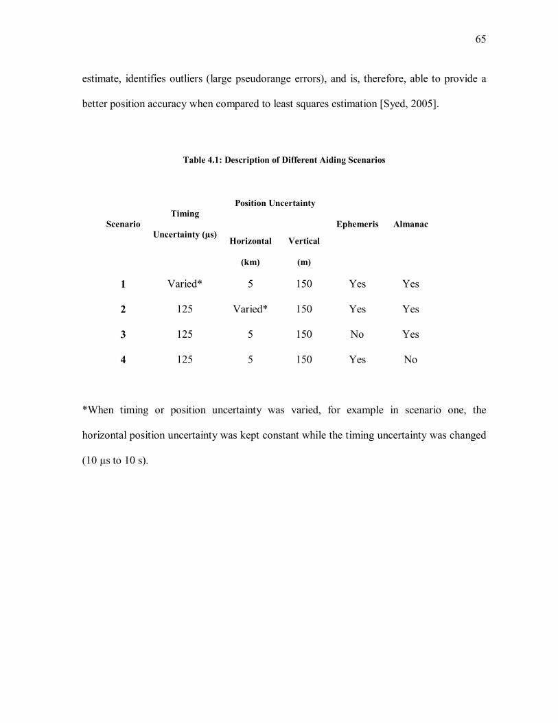
65

estimate, identifies outliers (large pseudorange errors), and is, therefore, able to provide a

better position accuracy when compared to least squares estimation [Syed, 2005].

Table 4.1: Description of Different Aiding Scenarios

Position Uncertainty

Scenario Timing

Uncertainty (µs) Horizontal

(km)

Vertical

(m)

Ephemeris Almanac

1 Varied* 5 150 Yes Yes

2 125 Varied* 150 Yes Yes

3 125 5 150 No Yes

4 125 5 150 Yes No

*When timing or position uncertainty was varied, for example in scenario one, the

horizontal position uncertainty was kept constant while the timing uncertainty was changed

(10 µs to 10 s).

66

Figure 4.1: Field Test Set-up for the AGPS Receiver

4.3 Field Test Environments

Cell phones are designed to work anywhere all the time. Field tests were carried in different

test sites where people may be using the cell phone for different purposes such as

emergency E-911 calls, personal navigation or commercial LBS applications. The tests

were conducted under many different conditions that would present various challenges such

as signal blockage or varying degree of signal attenuation. Acquisition tests were carried

out in the suburban environment, residential garage, inside a speed-skating track and a

concrete basement. The different test sites were chosen to determine the effects of various

factors on AGPS signal acquisition.

4.3.1 Suburban Environment

Acquisition tests were carried out at surveyed points at the University of Calgary campus

on October 9, 2004. The test site is shown in Figure 4.2, Figure 4.3 and Figure 4.4. There

was a tall glass building on the east side, a smaller concrete building on the west and a glass

67

walkway to the north. The southern side is unhindered with the exception of some

coniferous trees on the southwest side. The AGPS receiver was connected to a microstrip

patch antenna, which was placed at the test point as shown in Figure 4.2.

Figure 4.2: Receiver Setup for the Suburban Field Test

Figure 4.3: Reference Antenna and the Surrounding Site

68

Figure 4.4: Surrounding Area for the Test Site

4.3.2 Residential Garage

Acquisition tests were carried out in a residential garage with dimensions of 9 x 6 m x 2.5

m (located within 5 km from the University of Calgary) on December 9, 2004. The garage

setup, as shown in Figure 4.5 and Figure 4.6, is located underneath the living room of a

house and its walls are made of wood and concrete. The door facing the east side was made

of wood, while the wall facing the south side was partially constructed of wood. The

remaining two walls facing west and north were made of concrete. The garage door was

closed during all acquisition tests. The reference antenna was connected to the reference

receiver and located outside the garage. The AGPS receiver was connected to a microstrip

patch antenna, which was placed at a surveyed point inside the garage.

69

Figure 4.5: Test Setup for the Garage Test

Figure 4.6: Surrounding Area for the Garage Test

70

4.3.3 Speed-Skating Track

Acquisition tests were carried out on December 13, 2004 in a speed-skating track (see

Figure 4.7, Figure 4.8 and Figure 4.9), also known as the Olympic Oval, which is located

on the University of Calgary campus. The indoor speed-skating track is made of concrete

beams with approximate dimensions of 198 m x 80 m x 20 m. The roof is constructed with

corrugate steel (interior) and porcelain panels (exterior). The reference receiver was

connected to the reference antenna, which was placed near the window. The AGPS receiver

was connected to the microstrip patch antenna that was placed at a surveyed point inside

near the window because it was easier to obtain the position fix due to better satellite

availability.

Figure 4.7: Outside View of the Speed-skating Track

71

Figure 4.8: Receiver Setup for the Speed-skating Track Test

Figure 4.9: Inside the Speed-skating Track

72

4.3.4 Concrete Basement

An acquisition test as shown in Figures 4.10 and 4.11 was carried out in a concrete

basement with an underground pit inside. The dimensions of the pit are 7 m × 13 m × 4.5 m

and it is contained within a High Bay of 16 m × 14 m × 16 m. The test site is located inside

the CCIT building at the University of Calgary campus and the test was conducted on

November 30, 2004. The roof consists of a metal deck and steel structure. There is a door

located on the north side that is made of wood and on the northwest side there are two small

windows. The remaining three sidewalls were made of reinforced steel concrete. Similar to

the previous tests, the AGPS receiver was connected to a microstrip patch antenna that was

placed at a surveyed point inside the pit, while the reference antenna was kept outside.

Figure 4.10: Receiver Setup for the Concrete Basement Test

73

Figure 4.11: Surrounding Area for the Concrete Basement Test

4.4 High Sensitivity GPS Receiver

Limited field tests were carried out using the HSGPS receiver in the residential garage. A

HSGPS receiver was also used with the reference antenna on the CCIT roof. The results

obtained from the roof were similar to the suburban environment in terms of the TTTF

because of nominal GPS signals being present (see Section 4.8). The position results are

shown in Table 4.2 and Table 4.3. The position accuracy using thirty fixes was better for

the roof test (5.3 m) compared to the garage test (18.3 m). The roof had better satellite

availability and stronger LOS signals which resulted in better accuracy. The HSGPS

receiver could not acquire and/or obtain a position fix inside the speed-skating track and the

concrete basement because of very weak signals (< 25 dB-Hz). The TTFF for the HSGPS

receiver was ten times more than that of the AGPS receiver on the roof and six times more

in the residential garage. The TTFF in the residential garage test was seven times longer

74

when compared to the roof test. Simulation tests in Chapter 3 and Karunanayake et al.,

[2004] have shown that HSGPS was unable to acquire below -140 dBm which was further

confirmed during field tests. The TTFF increased when the simulator power decreased.

Research using HSGPS has shown longer TTFF with weaker signals during field tests

[Shewfelt at al., 2001]. The position accuracy also degraded with weaker GPS signals.

Further field tests using the AGPS receivers were carried out and results are discussed next

to illustrate the importance of assistance data.

Table 4.2: HSGPS Receiver- Position Results Using LSQ Internal Solution for Roof and

Garage Tests


Type of Environment 2D RMS

Error (m)

Mean # of

Satellites

2D RMS

Error (m)

Mean # of

Satellites

Roof 5.9 8.5 5.5 8.7

Residential Garage 19.9 5.5 18.3 4.3

Table 4.3: HSGPS Receiver- Position Results Using SiRF Internal Solution for Roof and

Garage Tests


Type of Environment 2D RMS

Error (m)

Mean # of

Satellites

2D RMS

Error (m)

Mean # of

Satellites

Roof 5.1 8.1 4.7 8.2

Residential Garage 22.8 4.3 18.9 3.9

75

4.5 Timing Assistance

This section will discuss results obtained from various aiding scenarios involving different

timing accuracies and the AGPS system. Timing assistance which was described in Section

2.4.3 can be used to narrow the acquisition search space. The tests aim to illustrate the

effects of accurate timing assistance under different test conditions. Syrjärinne and.

Kinnari, [2002] have shown using Location Measurement Units (LMUs), that the timing

accuracy of a GSM or UMTS network can range from a few microseconds to hundreds of

microseconds.


The TTFF results for precise and coarse time aiding are shown in Figure 4.12 and Figure

4.13. The position results that were obtained using the C3NAVG2 and the SiRF internal

solution are shown in Table 4.4, through to Table 4.7.

76

Figure 4.12: Precise Time Aiding - Normalized TTFF and Position Fixes for Suburban Test

Table 4.4: Precise Time- Position Results Using LSQ for Suburban Test

Five Position Fixes Thirty Position Fixes Precise Time

(µs) 2D RMS

Error (m)

Mean # of

Satellites

2D RMS

Error (m)

Mean # of

Satellites

10 40.4 5.6 35.4 6.1

50 47.6 4.9 39.3 5.9

125 60.8 5.6 60.1 5.7

250 44.3 6.2 47.3 6.4

500 57.5 5.0 54.5 6.4

77

Table 4.5: Precise Time Aiding - Position Results Using the SiRF Internal Solution Suburban Test


(µs) 2D RMS

Error (m)

Mean # of

Satellites

2D RMS

Error (m)

Mean # of

Satellites

10 32.3 5.1 28.5 6.3

50 30.3 5.2 27.3 6.2

125 61.3 5.3 69.3 6.1

250 28.5 5.3 25.1 7.0

500 26.4 5.3 24.2 6.5

Figure 4.13: Coarse Time Aiding- Normalized TTFF and Position Fixes for Suburban Test

78

Table 4.6: Coarse Time Aiding- Position Results Using LSQ for Suburban Test


Coarse Time

2D RMS

Error (m)

Mean #

of

Satellites

Tracked

2D RMS

Error (m)

Mean # of

Satellites

Tracked

1 ms 25.1 5.3 24.3 6.4

1 s 26.4 5.2 25.4 6.6

2 s 24.4 5.1 25.9 6.9

10 s 29.1 5.2 22.1 6.7

Table 4.7: Coarse Time Aiding- Position Results Using SiRF Internal Solution for Suburban Test


Coarse Time 2D RMS

Error (m)

Mean # of

Satellites

Tracked

2D RMS

Error (m)

Mean # of

Satellites

Tracked

1 ms 24.8 5.4 24.8 7.1

1 s 25.4 5.5 25.2 7.4

2 s 24.8 5.3 24.7 7.6

10 s 28.4 5.3 28.5 6.8

There was no variation or trends in the TTFF with varying timing uncertainty; however, the

TTFF was increased by 50% when the timing uncertainty changed to coarse time from

79

precise time aiding. The AGPS receiver was able to obtain a position fix for 100% of the

time during all the tests. The AGPS receiver used at least five or more satellites illustrating

very good availability. The SIRF internal compared to the LSQ solution showed better

position accuracy in terms of position accuracy because it uses Kalman filtering. The

position results with coarse time aiding showed similar position accuracies using the two

methods. The position results (SiRF solution) for five fixes, with the exception of 125 µs,

became better with increasing timing uncertainty (precise time aiding). The position

accuracy with coarse time aiding showed no trend. Generally the accuracy for thirty

position fixes was better than five position fixes because more satellite were used. More

satellite leads to better geometry or HDOP, which results in the improvement of user-

position accuracy. Acquisition is unpredictable in nature; possibilities exist where some

trials may have large position errors (satellites possibly tracking reflected signals). This

was the case for 125 µs where there were large errors which degraded the horizontal

position accuracy. The position errors were as large as 175 m for 125 µs, while the

maximum position error for 250 µs was 58 m. The TTTF increased with increasing time

uncertainty with coarse time aiding. However, the difference between the maximum and

minimum TTFF was only 2 s. This difference becomes significant when TTFF was

normalized because the average TTFF for most of the tests was 4 s.

Similar results in terms of trends in TTFF and position results were obtained when

simulation tests with varying time uncertainties (precise time) were carried out under

nominal signal conditions (-130 dBm) [Karunanayake, 2005b]. Simulation tests had also

shown that the position accuracy for the first few fixes was worse and improves as the code

80

tracking loops start getting better estimates of the position solution. The position accuracy

was better with increasing timing uncertainty. Garin et al., [2002] had also shown that first

fix at different signal levels was worse than the second fix.

The suburban environment, as shown in Figure 4.14, reflects that of nominal signal

conditions. The satellites generally had a C/N0 that was greater than 35 dB-Hz, however

there were some weak signals (28 dB-Hz) that may have been attenuated due to signal

masking from coniferous trees. The C/N0 PDF (at different elevations) plot was obtained

using all the data from the 125 µs test. A similar method was used to obtain the C/N0 plot

for the other environments. PRNs 6 and 9 were lower elevation satellites located on the

south side and were attenuated by trees. The remaining three satellites were higher

elevation and therefore did not suffer from signal blockage or attenuation. Similar results

were obtained in Hu, [2006] and MacGougan, [2003].

Figure 4.14: C/N0 PDF for the Suburban Test

81


The results for the residential garage for precise and coarse time aiding are shown in Figure

4.15 and Figure 4.16. The position results that were obtained using C3NAVG2 and the SiRF

internal software are shown in Table 4.8 through Table 4.11

Figure 4.15: Precise Time Aiding – Normalized TTFF and Position Fixes for Garage Test

82

Table 4.8: Precise Time Aiding - Position Results Using LSQ for the Garage Test


Precise Time

(µs)

2D RMS

Error (m)

Mean # of

Satellites

Tracked

2D RMS

Error (m)

Mean # of

Satellites

Tracked

10 16.8 3.7 23.1 4.1

50 27.2 3.8 23.0 3.9

125 19.0 3.5 23.5 4.5

250 15.4 3.6 29.7 5.6

500 16.5 4.2 21.9 4.1

Table 4.9: Precise Time Aiding - Position Results Using SiRF Internal Solution for Garage Test


Precise Time

(µs)

2D RMS

Error (m)

Mean # of

Satellites

Tracked

2D RMS

Error (m)

Mean # of

Satellites

Tracked

10 25.4 5.3 19.4 5.2

50 24.9 5.3 25.5 5.2

125 18.8 5.1 20.7 5.0

250 18.3 5.0 23.9 5.4

500 17.7 5.2 26.9 5.3

83

Figure 4.16: Coarse Time Aiding – Normalized TTFF and Position Fixes for Garage Test

Table 4.10: Coarse Time Aiding - Position Results Using LSQ for Garage Test


Coarse Time 2D RMS Error

(m)

Mean # of

Satellites

2D RMS

Error (m)

Mean # of

Satellites

1 ms 23.5 3.1 20.2 3.1

1 s 31.9 3.8 27.6 4.1

2 s 30.7 4.2 20.2 3.8

10 s 18.4 4.5 24.1 4.4

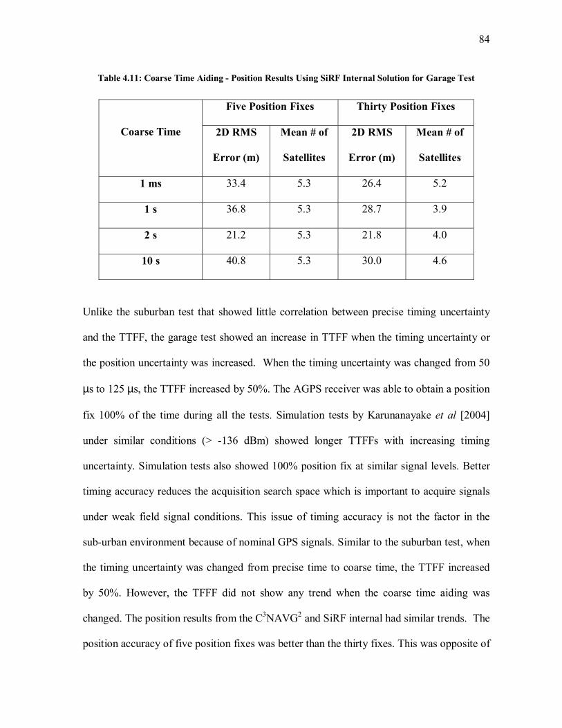
84

Table 4.11: Coarse Time Aiding - Position Results Using SiRF Internal Solution for Garage Test


Coarse Time 2D RMS

Error (m)

Mean # of

Satellites

2D RMS

Error (m)

Mean # of

Satellites

1 ms 33.4 5.3 26.4 5.2

1 s 36.8 5.3 28.7 3.9

2 s 21.2 5.3 21.8 4.0

10 s 40.8 5.3 30.0 4.6

Unlike the suburban test that showed little correlation between precise timing uncertainty

and the TTFF, the garage test showed an increase in TTFF when the timing uncertainty or

the position uncertainty was increased. When the timing uncertainty was changed from 50

µs to 125 µs, the TTFF increased by 50%. The AGPS receiver was able to obtain a position

fix 100% of the time during all the tests. Simulation tests by Karunanayake et al [2004]

under similar conditions (> -136 dBm) showed longer TTFFs with increasing timing

uncertainty. Simulation tests also showed 100% position fix at similar signal levels. Better

timing accuracy reduces the acquisition search space which is important to acquire signals

under weak field signal conditions. This issue of timing accuracy is not the factor in the

sub-urban environment because of nominal GPS signals. Similar to the suburban test, when

the timing uncertainty was changed from precise time to coarse time, the TTFF increased

by 50%. However, the TFFF did not show any trend when the coarse time aiding was

changed. The position results from the C3NAVG2 and SiRF internal had similar trends. The

position accuracy of five position fixes was better than the thirty fixes. This was opposite of

85

what was observed in the suburban environment. During thirty fixes the number satellites

used would vary (three to five), which would change the HDOP, and, in fact, could degrade

the position accuracy. For example, time aiding of 125 µs showed a maximum position

error for five fixes of 37 m, while it was 176 m for thirty fixes. The position accuracy (SiRF

solution for five fixes) improved with decreasing timing uncertainty (precise) but did not

show any trends with coarse time aiding. These trends in position results were similar to the

suburban environment.

Most of the signals experienced signal attenuation (see Figure 4.17) but some satellites such

as PRNs 19 and 27 had strong signals (C/N0 greater than 30 dB-Hz). The weakest satellite

(PRN 29) had a C/N0 of 21.4 dB-Hz. Higher signal attenuation would be caused by

building materials such as concrete walls while some stronger signals may experience

moderate attenuation from wooden surfaces. The trends between elevation is not clear

unlike the sub-urban test were higher elevation satellites had stronger signals. Other factors

such as different surfaces (wood or concrete), that is signal attenuation determines the

signal strength.

86

Figure 4.17: C/N0 PDF for the Residential Garage Test

4.5.3 Speed-skating Track

The speed-skating track results using different timing uncertainties are shown in Figure

4.18. The position results that were obtained using C3NAVG2 and the SiRF internal

software are shown in Table 4.12 and Table 4.13. Acquisition tests with coarse aiding were

carried out using 1 ms. Tests with other timing levels could not be carried out on that day so

they are not shown.

87

Figure 4.18: Precise Time Aiding – Normalized TTFF and Position Fixes for Speed-skating Test

Table 4.12: Precise Time - Aiding Position Results Using LSQ for Speed-skating Test


(µs) 2D RMS

Error (m)

Mean # of

Satellites

2D RMS

Error (m)

Mean # of

Satellites

10 55.1 3.6 46.7 3.8

50 49.0 3.5 45.4 3.4

125 58.4 3.9 59.1 3.9

250 46.6 3.3 43.3 3.2

500 57.5 4.1 47.9 4.0

88

Table 4.13: Precise Time Aiding - Position Results using SiRF Internal Solution for Speed-skating Test


Precise Time (µs) 2D RMS

Error (m)

Mean # of

Satellites

2D RMS

Error (m)

Mean # of

Satellites

10 54.0 5.3 57.7 4.7

50 57.8 5.3 48.8 4.6

125 45.7 3.7 37.5 3.8

250 45.5 5.8 49.3 3.4

500 60.1 5.3 59.8 3.4

Similar to the residential garage test results, the results here with precise time aiding show a

definite trend. For example, when the timing uncertainty was changed from 50 to 125 µs,

the TFFF increased by 83%. The results are similar to the residential garage tests

illustrating the importance of good timing accuracy. The position fix success rate also

decreased with increasing timing uncertainly. The success rate was 100% for 10 µs and 50

µs but decreased from 95% to 85% when the timing uncertainty was changed from 125 µs

to 500 µs. These results are different from those of the residential garage which had 100%

success rate for all the tests. Similarly, simulations tests carried out at weak power (-152

dBm) had a success rate of 80% [Karunanayake, 2000b]. Acquisition is difficult to carry

out with weaker signals especially when the timing uncertainty is increased, since weaker

signals prolong the search process (longer integration time). In many instances the receiver

is unable to find the GPS signals before the required time of 300 s. When the time aiding

was changed from precise to coarse, 500 µs to 1 ms, the TTFF increased by 150%. The

89

position accuracy using C3NAVG2 was better for five position fixes than thirty fixes

(similar to the suburban environment). The SiRF solution did not show any trend between

five and thirty position fixes. Unlike, the other two environments the position accuracy did

not show any trend with precise time aiding.

The speed-skating track suffered from significant blockage which reduced satellite

availability (usually less than four satellites). Therefore, the solution using C3NAVG2 was

obtained by fixing the height. Height fixing would require three rather than four

observations to solve for the three unknowns (horizontal position and time). Generally the

AGPS receiver would use anywhere from three to five satellites to obtain a position fix. The

speed-skating track had very weak signals (see Figure 4.19). Most of the satellites had

signal strength less than 25 dB-Hz. The signals are highly attenuated by materials such as

concrete walls. However, there was one satellite with strong signals (possibly entering

through a glass window, PRN 5 with C/N0 of 29.9 dB-Hz).

Figure 4.19: C/N0 PDF for the Speed-skating Track Test

90


The concrete basement results are shown in Figure 4.20 and Figure 4.21 and the position

results obtained using the C3NAVG2 and SiRF internal solutions are shown in Table 4.14

through Table 4.17.

Figure 4.20: Precise Time Aiding – Normalized TTFF and Position Fixes for Concrete Basement Test

91

Table 4.14: Precise Time Aiding - Position Results using LSQ Concrete Basement Test


Precise Time (µs) 2D RMS Error

(m)

Mean # of

Satellites

2D RMS

Error (m)

Mean # of

Satellites

10 60.1 3.7 49.6 3.7

50 61.0 3.8 78.2 3.9

125 61.7 4.9 68.4 3.5

250 54.5 4.8 55.0 4.1

500 43.0 5.1 77.0 3.0

Table 4.15: Precise Time Aiding - Position Results using SiRF internal Solution for Concrete Basement

Test


Precise Time (µs) 2D RMS

Error (m)

Mean # of

Satellites

2D RMS

Error (m)

Mean # of

Satellites

10 74.7 5.2 70.6 4.7

50 59.6 5.1 57.3 4.0

125 58.5 5.3 56.2 3.6

250 55.4 5.4 53.2 3.6

500 58.6 5.3 71.6 3.2

92

Figure 4.21: Coarse Time Aiding – Normalized TTFF and Position Fixes for Concrete Basement Test

Table 4.16: Coarse Time Aiding - Position Results Using LSQ for Concrete Basement Test


Coarse Time 2D RMS

Error (m)

Mean # of

Satellites

2D RMS

Error (m)

Mean # of

Satellites

1 ms 44.6 4.4 65.8 4.4

1 s 62.3 4.8 45.0 4.7

2 s 44.6 4.3 65.8 4.1

10 s 57.5 5.1 68.3 4.8

93

Table 4.17: Coarse Time Aiding - Position Results using SiRF Internal Solution for Concrete Basement

Test


Coarse Time 2D RMS

Error (m)

Mean # of

Satellites

2D RMS

Error (m)

Mean # of

Satellites

1 ms 60.1 5.3 57.4 3.2

1 s 42.1 5.3 37.0 3.6

2 s 43.4 5.3 37.6 3.2

10 s 55.5 5.0 56.8 3.2

Similar to the field tests that were carried out in the residential concrete garage and the

speed-skating track, when timing uncertainty (precise time aiding) was increased in the

concrete basement, this led to an increase in the TTFF. For example, when the timing

uncertainty was changed from 50 µs to 125 µs, the TTFF increased by 100%. The trend is

similar to the previous two weak signal indoor environments; longer timing certainty results

in longer search time or longer TTFF. When the timing uncertainty was changed to coarse

time from precise time, the TTFF increased by 10%, however similar to the residential

garage test, there was no observable trend between the different timing uncertainties

(coarse) and TTFF. The success rate decreased with increasing timing uncertainty. For

example, when the timing uncertainty was changed from 50 to 500 µs, the percentage of

successful position fixes decreased from 95% to 50%. It dropped even further, to 45%,

when the timing uncertainty was changed to 10 s. The success rate at 500 µs was better for

the speed-skating track (85%) because all the signals in the concrete basement were highly

94

attenuated. The results illustrate the increased difficulty in obtaining a position fix or

finding the GPS signal in an environment which has all weak signals. Similar results were

obtained when acquisition tests using the simulator were carried out where all satellites had

same power level of -145 dBm [Karunanayake, 2005b].

Similar to the speed-skating track, the receiver in the concrete basement would track or use

an average of three satellites. Therefore, the use of height constraints when obtaining the

position solution using C3NAVG2 was required. The position obtained using the two

methods had similar results in terms of position accuracy. The results did not show any

trends between five and thirty position fixes. Similar to the suburban environment and

residential garage, the position accuracy (both methods using five fixes) improved with

decreasing timing uncertainty.

The satellites had highly attenuated signals in the concrete basement with signal strengths

less than 22 dB-Hz, with the exception of one satellite (see Figure 4.22). The concrete

basement had very limited LOS signals (small window). Signals generally entered from

concrete walls and were, therefore, highly attenuated.

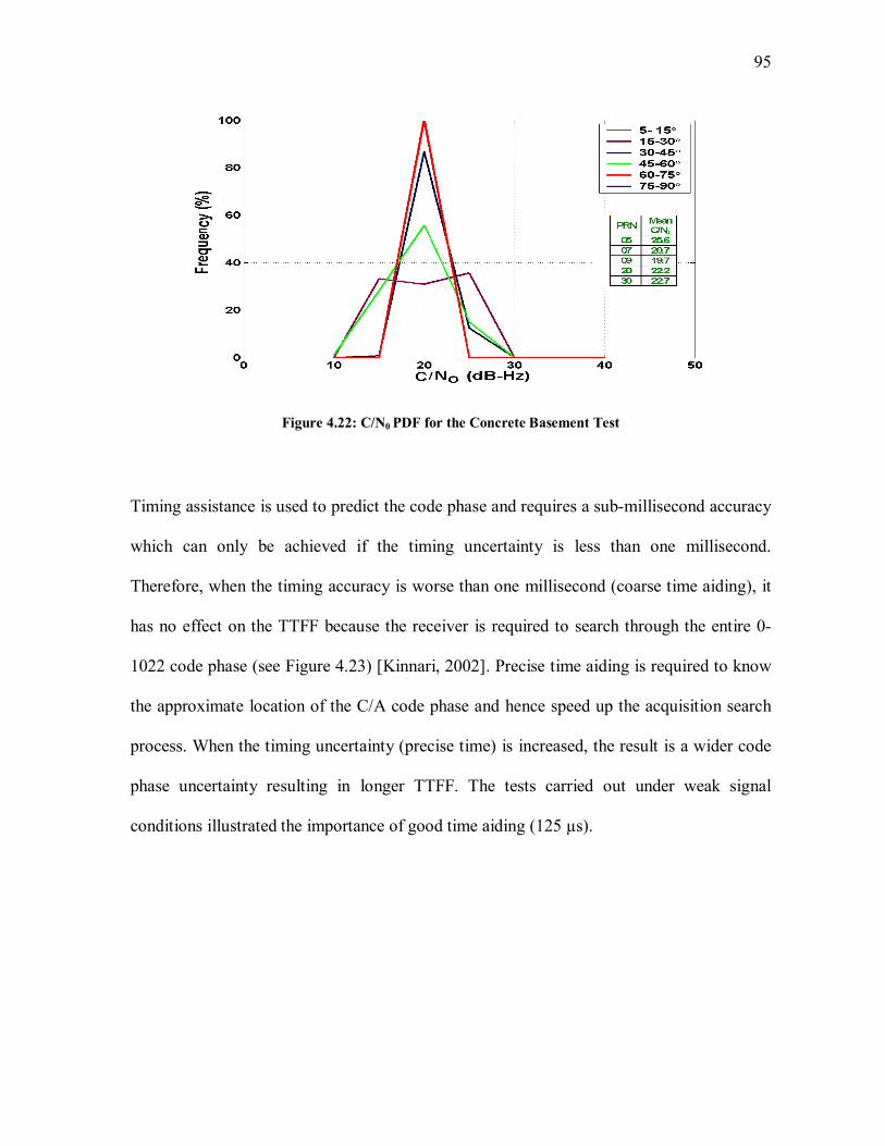
95

Figure 4.22: C/N0 PDF for the Concrete Basement Test

Timing assistance is used to predict the code phase and requires a sub-millisecond accuracy

which can only be achieved if the timing uncertainty is less than one millisecond.

Therefore, when the timing accuracy is worse than one millisecond (coarse time aiding), it

has no effect on the TTFF because the receiver is required to search through the entire 0-

1022 code phase (see Figure 4.23) [Kinnari, 2002]. Precise time aiding is required to know

the approximate location of the C/A code phase and hence speed up the acquisition search

process. When the timing uncertainty (precise time) is increased, the result is a wider code

phase uncertainty resulting in longer TTFF. The tests carried out under weak signal

conditions illustrated the importance of good time aiding (125 µs).

96

Figure 4.23: Time Relationship for L1 C/A Code [Source: Kaplan and Hegarty, 2006]

4.6 Horizontal Position Assistance

Horizontal position assistance can be sent to the mobile device via a wireless network, such

as CDMA or GSM. The GSM network would use the E-OTD method to obtain a position

[Syrjärinne and Kinnari, 2002]. The cell size could be as small as 3 km in urban centres and

as large as 30 km in rural areas. The user position assistance is used to determine the visible

satellites and the combination of timing and position assistance can be used to predict the

approximate C/A code phase. The values of horizontal position uncertainties were chosen

97

to reflect the cell site size. Although a cell site would never be as large as 350 km, a

position uncertainty of this magnitude was used because an uncertainty of greater than 300

km with exact timing assistance will force a complete sweep of the entire 1023 code chips

[Kinnari, 2002]. The results were quantified using factors such as TTFF, 2-D position

accuracy (vertical position accuracy was not considered, the height assistance was kept

constant) and number of satellites tracked. The following sections discuss the results

obtained in the four field environments.


Acquisition tests were carried out using different horizontal position uncertainties and the

results with TTFF and position fixes are shown in Figure 4.24. The position results that

were obtained from the C3NAVG2 and SiRF internal solutions are shown in Table 4.18 and

Table 4.19.

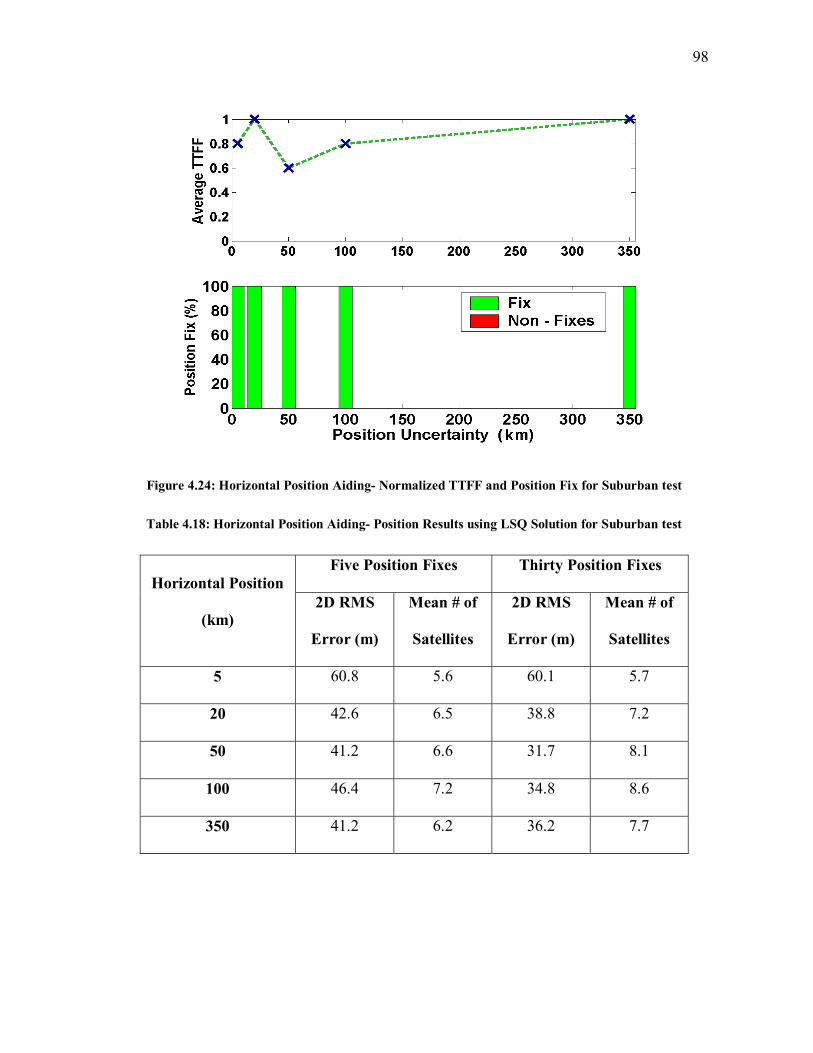
98

Figure 4.24: Horizontal Position Aiding- Normalized TTFF and Position Fix for Suburban test

Table 4.18: Horizontal Position Aiding- Position Results using LSQ Solution for Suburban test

Five Position Fixes Thirty Position Fixes Horizontal Position

(km) 2D RMS

Error (m)

Mean # of

Satellites

2D RMS

Error (m)

Mean # of

Satellites

5 60.8 5.6 60.1 5.7

20 42.6 6.5 38.8 7.2

50 41.2 6.6 31.7 8.1

100 46.4 7.2 34.8 8.6

350 41.2 6.2 36.2 7.7

99

Table 4.19: Horizontal Position Aiding- Position Results for SiRF Internal Solution for Suburban Test


(km) 2D RMS

Error (m)

Mean # of

Satellites

2D RMS

Error (m)

Mean # of

Satellites

5 61.3 5.3 69.3 6.1

20 40.7 6.6 40.4 7.6

50 37.3 7.0 30.1 8.1

100 35.3 7.6 39.5 8.8

350 31.0 6.8 33.0 7.9

Similar to the tests that were carried out using timing assistance, the tests with varying

horizontal assistance failed to show any trends with respect to TTFF. The AGPS receiver

was able to obtain a position fix successfully 100% of the time. The TTFF for 50 km was

40% worse than 20 km, however when using units of time the difference was only 2 s. The

receiver used an average of seven satellites to compute the position solution using the two

methods that showed similar results in terms of horizontal position accuracy. The position

accuracy was better for thirty position fixes. There were more satellites used for thirty fixes.

The HDOP or geometry generally improves with more satellites under nominal signal

conditions. The position accuracy also improved with larger position uncertainty because

more satellites were used to obtain the position solution. Simulation tests had not shown

any trend with varying position assistance because the number of satellites used was

constant [Karunanayake, 2005b].

100


Similar tests using different position uncertainties were carried out in the residential garage.

The TTFF for various position uncertainties are shown in Figure 4.25 and the position

results are shown in Table 4.20 and Table 4.21.

Figure 4.25: Horizontal Position Aiding- Normalized TTFF and Position Fix for Garage Test

101

Table 4.20: Horizontal Position Aiding- Position Results using LSQ Solution for Garage Test


(km) 2D RMS

Error (m)

Mean # of

Satellites

2D RMS

Error (m)

Mean # of

Satellites

5 19.0 3.5 23.5 4.5

20 56.3 4.3 37.1 4.7

50 45.1 5.3 56.7 4.9

100 25.2 4.7 40.4 4.5

350 43.1 3.0 50.7 3.9

Table 4.21: Horizontal Position Aiding- Position Results for SiRF Internal Solution for Garage Test


(km) 2D RMS

Error (m)

Mean # of

Satellites

2D RMS

Error (m)

Mean # of

Satellites

5 18.8 5.1 20.7 5.0

20 44.8 5.1 31.8 5.0

50 61.5 5.4 35.2 4.1

100 61.0 5.4 46.5 4.8

350 52.0 5.2 42.6 3.8

Unlike the suburban test that did not show any trend between the position uncertainty and

TTFF, the tests in the garage showed that when the horizontal position uncertainty

102

increased, so did the TTFF. For example, when the position uncertainty was changed from

20 km to 100 km, the TTFF increased by 100% and the receiver was able to obtain a

position fix 100% of the time. Position assistance and accurate timing information can be

used to predict the approximate C/A code phase. However, unlike timing assistance,

position assistance with ephemeris can be used to predict the approximate satellite Doppler.

It has been shown in van Diggelen, [2001] that an uncertainty of one kilometre will result in

a Doppler error of one Hertz. Higher uncertainty in position would result in larger search

space (C/A code and Doppler), resulting in longer search time or TTFF.

The two position solutions used an average of at least four satellites with similar horizontal

position accuracy. The position results did not show any trends between five and thirty

positions fixes or with different horizontal position uncertainty. The number of satellites

was similar for different tests (three to five). The tests with varying horizontal position

aiding using the simulator also did not show any trends in position results [Karunanayake,

2005b]. The TTFF increased with decreasing horizontal position aiding under weak signal

conditions (-140 dBm).

4.6.3 Speed-skating Track

The TTFFs for various position uncertainties are shown in Figure 4.26 and the

corresponding position results using C3NAVG2 and SiRF software are shown in

Table 4.22 and Table 4.23.

103

Figure 4.26: Horizontal Position Aiding – Normalized TTFF and Position Fix for Speed-skating Test

Table 4.22: Horizontal Position Aiding- Position Results using LSQ Solution for Speed-skating Test


(km) 2D RMS

Error (m)

Mean # of

Satellites

2D RMS

Error (m)

Mean # of

Satellites

5 58.4 3.9 59.1 3.9

20 43.2 3.3 42.2 3.6

50 59.7 3.6 43.8 3.4

100 57.6 4.0 45.9 4.9

350 51.8 4.5 45.2 5.1

104

Table 4.23: Horizontal Position Aiding- Position Results for SiRF Internal Solution for Speed-skating

Test


(km) 2D RMS

Error (m)

Mean # of

Satellites

2D RMS

Error (m)

Mean # of

Satellites

5 45.7 3.7 37.5 3.8

20 34.1 5.5 36.1 4.3

50 40.9 5.5 41.0 4.4

100 50.8 5.4 50.6 4.9

350 46.2 5.3 38.2 5.4

Similar to the garage test, acquisition tests in the speed-skating track showed that increasing

the horizontal position uncertainty led to a longer TTFF For instance, when the position

uncertainty was changed from 20 to 50 km, the TTFF increased by 50%. However, unlike

the garage test, increasing the position uncertainty resulted in a decrease in the success rate

for obtaining a position fix. For example, when the position uncertainty was changed from

20 km to 100 km the success rate decreased from 92% to 82%. The results are similar to

tests that were carried out using different time aiding. It is difficult to search GPS signals

under extremely weak signal conditions. When the position uncertainty is large, a larger

Doppler and C/A search space is the result. The receiver could be searching in the wrong

search bin and is unable to find the GPS signal before the required time of 300 s.

105

The AGPS receiver used at least three satellites to obtain the C3NAVG2 solution for most of

the tests. The SiRF internal solution however used an average of four satellites and had

better horizontal position accuracy because of better satellite availability. Similar to the

residential garage test, there were no observable trends between five and thirty position

fixes or different position aiding values.


Finally tests using different position uncertainties were carried out in the concrete

basement. The TTFFs using different position uncertainties are shown in Figure 4.27, while

the position results are shown in Table 4.24 and Table 4.25.

Figure 4.27: Horizontal Position Aiding – Normalized TTFF and Position Fix for Concrete Basement

106

Table 4.24: Horizontal Position Aiding– Position Results using LSQ Solution for Concrete Basement


(km) 2D RMS

Error (m)

Mean # of

Satellites

2D RMS

Error (m)

Mean # of

Satellites

5 61.7 5.3 68.4 3.2

20 67.5 4.5 58.5 3.3

50 48.7 4.2 86.4 3.2

100 86.0 4.4 104.1 3.4

350 62.6 4.3 62.3 2.9

Table 4.25: Horizontal Position Aiding– Position Results for SiRF Internal Solution for Concrete

Basement


(km) 2D RMS

Error (m)

Mean # of

Satellites

2D RMS

Error (m)

Mean # of

Satellites

5 58.5 5.3 56.2 3.6

20 45.5 5.1 42.8 3.2

50 69.1 5.4 75.1 3.3

100 54.3 5.2 58.6 3.2

350 46.3 5.3 56.1 2.7

107

Similar to acquisition tests that were carried out in the residential garage and the speed-

skating track, increasing the position uncertainty led to longer TTFFs here as well. For

example, when the position uncertainty was changed from 50 km to 100 km, the TTFF

increased by 40%. When the position aiding was changed from 20 km to 50 km the TTFF

dropped by about four seconds. Since the TTFF was in hundreds of seconds, this small drop

is not particularly significant. Similar to the speed-skating test, increasing the position

uncertainty led to a decrease in the success rate. For instance, when the position uncertainty

was changed from 20 km to 100 km the success of position fixes decreased from 85% to

72%. The success rate was better for the speed-skating track (82% for 100 km) when

compared to the concrete basement test. The speed-skating track has one strong signal

which is initially acquired and later used to acquire the remaining weaker satellites. In the

concrete-basement all the signals are weak therefore takes a longer time to acquire. In many

instances it is not possible to acquire or obtain a position fix during the required time. The

concrete-basement is in fact a very harsh environment. This can be illustrated by the fewer

number of satellites tracked or used by the two methods (position solutions) and the poor

position accuracy. The position results obtained with both methods was similar, with SiRF

solution providing slightly better position accuracy. Similar to the speeds-skating track and

residential garage the position results did show any trends for position aiding scenarios.

108

4.7 Ephemeris and Almanac Assistance

When the mobile station knows the approximate user location and is aware of the current

GPS time, visible satellites can be determined if the satellite ephemeris is sent to the mobile

via a wireless network. In all of the above tests, the satellite ephemeris and almanac were

provided to the AGPS receiver. In the following tests, the satellite ephemeris or almanac

will be withheld from the AGPS receiver. Simulation tests have already demonstrated the

importance of satellite ephemeris in terms of factors such as lower TTFF and better

acquisition sensitivity.

Acquisition tests were carried out using scenarios three and four (see Table 4.1) in the four

different field test environments. In scenario three the receiver does not get any ephemeris

while in scenario four the receiver does not get almanac. The timing and horizontal

uncertainty were kept at 125 µs and 5 km for both scenarios. The position results using

C3NAVG2 and the SiRF internal solution are shown in Table 4.26 and Table 4.27.

109

Table 4.26: Ephemeris or Almanac Aiding- Position Results Aiding Using LSQ for all the Test Sites


2D RMS

Error (m)

Mean # of

Satellites

2D RMS

Error (m)

Mean # of

Satellites

Almanac 41.4 6.7 35.9 7.2 Suburban

Ephemeris 49.4 7.1 40.4 6.7

Almanac 25.9 5.3 25.2 6.2 Residential

Garage Ephemeris 21.3 5.2 18.5 6.4

Almanac 57.9 3.4 55.4 3.3 Speed-

skating

Track Ephemeris X X X X

Almanac 63.2 4.1 56.1 3.4 Concrete

Basement Ephemeris X X X X

110

Table 4.27: Ephemeris or Almanac Aiding - Position Results Using SiRF Internal Solution for all the

Test Sites


2D RMS

Error (m)

Mean # of

Satellites

2D RMS

Error (m)

Mean # of

Satellites

Almanac 46.7 6.8 41.6 7.3 Suburban

Ephemeris 21.0 7.3 35.4 6.8

Almanac 27.0 5.3 23.0 6.4 Residential

Garage Ephemeris 31.2 5.3 27.2 6.6

Almanac 62.9 3.6 61.9 3.6 Speed-

skating

Track

Ephemeris X X X X

Almanac 45.8 4.2 37.5 4.5 `Concrete

Basement Ephemeris X X X X

X – Acquisition or position fix could not be obtained

The acquisition test results show that the AGPS receiver was able to perform signal

acquisition without ephemeris in the suburban and residential garage but not in the speed-

skating track or concrete basement. The TTFF was ten times more for the suburban test and

six times more for the residential garage when compared with time (125 µs) and horizontal

position aiding (5 km). The position results were similar to the ones that were obtained

using different time and position aiding.

111

Acquisition tests could not be carried out in the other two environments (speed-skating

track and the concrete basement). This further confirms the simulation tests, where the

AGPS receiver (without ephemeris) was unable to acquire signals below -142 dBm.

The acquisition tests without almanac assistance had the same TTFF when compared with

the time and position assistance of 125 us and 5 km for all four test environments. If the

receiver does not have ephemeris, it will download satellite ephemeris and this can take up

to 30 seconds. This prolongs the search process resulting in longer TTFFs. The satellite

almanac, unlike satellite ephemeris, provides coarse information for such things as satellite

orbits and, therefore, is not required for signal acquisition.

4.8 Comparison of Different Environments

This section compares the acquisition performance of the AGPS receiver in the four

different environments. The roof-top receiver is again used as a reference since there are

strong LOS signals (43 to 45 dB-Hz) present on the roof-top. All the other tests can be

referenced to the roof test. The results for different precise time aiding and horizontal

position assistance are shown in Figure 4.28 and Error! Reference source not found.. The

position results obtained from C3NAVG2 are given in Table 4.28 where the AGPS receiver

received ephemeris, almanac; time aiding of 125 µs uncertainty and position assistance of 5

km uncertainty.

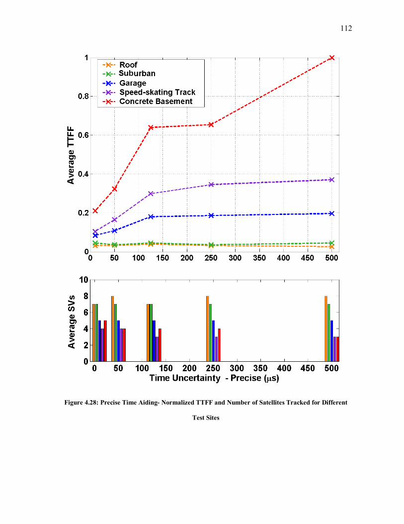
112

Figure 4.28: Precise Time Aiding- Normalized TTFF and Number of Satellites Tracked for Different

Test Sites

113

Figure 4.29: Horizontal Position Aiding- Normalized TTFF and Number of Satellites for Different Test

Sites

114

Table 4.28: Position Results Using LSQ Solution Under Different Field Test Conditions


Different Field

Test Sites

2D

RMS

Error

(m)

Mean #

of

Satellites

Mean

HDOP

2D

RMS

Error

(m)

Mean #

of

Satellites

Mean

HDOP

Roof 3.6 8.2 1.1 3.8 7.9 1.2

Suburban

Environment 60.8 5.6 3.5 60.1 5.7 3.2

Residential

Garage 18.8 5.1 1.3 23.5 5.0 1.6

Speed-skating

Track

45.7 3.7 4.2 37.5 3.8 3.9

Concrete

Basement 61.7 5.3 2.7 68.4 3.2 3.5

The trends between the timing and position assistance showed similar results with the

number of satellites tracked and the TTFF. The TTFF between two different environments

are compared using time aiding of 125 µs and position uncertainty of 5 km. The TTFFs of

the roof test showed a similar trend when compared to the suburban environment. Both test

sites had nominal signal conditions (39 to 45 dB-Hz). Position accuracy was worse in the

suburban environment, which could be due to a lower number of satellites used. A lower

115

number of satellites results in poorer geometry or multipath effects (glass building would

cause strong specular reflections). The residential garage had attenuated signals (30 dB-Hz)

with TTFFs which were five times longer than the suburban environment. However, the

AGPS receiver had better position accuracy due to factors such as better geometry (HDOP

was 1.6, less than suburban which had HDOP of 3.2), and multipath from diffuse sources

may not be as severe as that due to specular reflective sources. Similarly, the speed-skating

environment with signal strength of 25 dB-Hz had a TTFF that was twice as long as that of

the residential garage. The speed-skating environment also had poor position accuracy that

could be due to factors such as poor geometry and strong specular reflections due to the

corrugated roof for example. Although the concrete basement and the speed-skating track

had similar signal conditions however, the signal in the concrete basement was 5 dB lower

(see Figure 4.19 and Figure 4.22), the TTFF was twice as long for the concrete basement.

This was the case because the test in the speed-skating track was carried out near a window

where there was one strong satellite (PRN 5). Simulation tests and Karunanayake [2005b]

have shown the importance of initially acquiring a strong satellite that can then be used to

aid in acquiring the remaining weaker satellites. Once the first strong satellite is acquired, it

can be used to provide such things as accurate GPS timing and clock bias, which can be

used to acquire the remaining weaker satellites. The results have shown that it takes a

longer period of time to acquire a signal in weaker signal conditions. Weaker signals imply

a longer search time or integration time and, thus, a longer TTFF [Shewfelt et al., 2001].

Typically coherent integration is kept constant while non-coherent integration is changed to

acquire signal at different power levels.

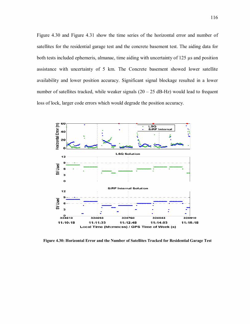
116

Figure 4.30 and Figure 4.31 show the time series of the horizontal error and number of

satellites for the residential garage test and the concrete basement test. The aiding data for

both tests included ephemeris, almanac, time aiding with uncertainty of 125 µs and position

assistance with uncertainty of 5 km. The Concrete basement showed lower satellite

availability and lower position accuracy. Significant signal blockage resulted in a lower

number of satellites tracked, while weaker signals (20 – 25 dB-Hz) would lead to frequent

loss of lock, larger code errors which would degrade the position accuracy.

Figure 4.30: Horizontal Error and the Number of Satellites Tracked for Residential Garage Test

117

Figure 4.31: Horizontal Error and the Number of Satellites Tracked for Concrete Basement Test

4.9 Comparison of Simulation & Field Tests

Simulation tests were carried out in a controlled environment where every satellite had the

same power unlike field test conditions where the signal power varied due to various factors

such signal attenuation, and signal blockage or reflected signals coming from different

types of surfaces. No measurement errors such as multipath were simulated. Field tests

however were subject to multipath effects which would affect the position accuracy. Signal

blockage reduces satellite visibility which would lead to poor geometry or HDOP which

118

would also degrade the position accuracy. During simulation tests the number of satellites is

kept constant and, therefore, signal blockage is not a problem. The results using the two

methodologies showed similar trends in TTFF and acquisition sensitivity. The trends in the

TTFF depend on the signal strength and were, therefore, easier to observe. Research by El-

Natour et al., [2005] has shown that multipath does not affect signal acquisition in terms of

TTFF.

The trends in position were difficult to observe because there are other factors such as

multipath which affect the position accuracy during various field tests. The only factor in

the simulator tests that would affect the position accuracy was different signal power level.

Simulation tests with different time aiding showed that position accuracy became better

with increased time uncertainty [Karunanayake, 2005b]. Field tests have shown that trend

for the first two environments (suburban environment and residential garage), however the

last two environments which had very weak signals did not show any trends. Simulation

and field tests however did not show any trend between varying horizontal position

uncertainty and the position results.

4.10 Chapter Summary

Acquisition field tests using a HSGPS receiver and AGPS receiver were carried out at

various test sites. Conclusions drawn from the field tests are discussed below.

119

• The acquisition field tests showed the limitations of the HSGPS receiver: its

inability to acquire in weak signal conditions and long TTFF (ten times longer)

when compared to the AGPS receiver.

• The acquisition field tests showed that lack of satellite ephemeris resulted in longer

TTFF, while that the almanac is not required for signal acquisition

• Increased timing uncertainty (precise time aiding) results in longer TTFF under

weak signal conditions. The tests also showed that sub-millisecond level accuracy

for the time aiding is required. In other words, coarse time aiding has no effect on

TTFF.

• The tests under different field test conditions showed the increasing level of

difficulty in acquiring satellite signals or obtain a position, especially in

environments such as the speed-skating track and the concrete basement. These two

environments had highly attenuated signals (20 to 25 dB-Hz). The position accuracy

using the two methods (SiRF internal and least squares) was less than 50 m for the

first two environments (suburban and residential garage)but was worse for the last

two environments (speed-skating track and concrete basement, less than 70 m). The

position accuracy was better than E-OTD (100 m) and within the maximum

requirement of 150 m for the FCC-E911 mandate.

120

CHAPTER 5: FIELD TESTS: TRACKING

This chapter discusses the test objectives, methodologies and results that were obtained for

tracking tests at different test sites. The test sites were the same ones used in Chapter Four

to conduct acquisition tests. The chapter also provides analysis under different test

conditions and provides some conclusions that can be drawn from various tracking tests.

5.1 Test Objectives

Tracking tests were conducted in different field test conditions to meet the following test

objectives.

• Compare the performance of HSGPS and AGPS under weak or degraded field test

conditions

• Determine the effects of aiding data on tracking performance of the AGPS receiver

5.2 Field Test Methodology

Tracking tests (see Figure 5.1) that were carried out inside a building required an

initialization of twenty minutes under open sky conditions to ensure that the receivers had

the complete satellite almanac and ephemeris [MacGougan, 2003]. The AGPS receiver is

able to acquire signals indoors; however, initialization was carried with both the HSGPS

and AGPS receivers to keep the methodology consistent. The reference receiver provided

121

aiding data (timing (125 µs), position uncertainty (5 km), and satellite ephemeris and

almanac) to the AGPS receiver. The tests were carried out to illustrate the effects of

multipath, signal blockage, and signal attenuation on solution accuracy and availability

under different field test conditions. The tracking tests were analyzed through the

horizontal and vertical errors, number of satellites used in the position solution, C/N0 and

measurement residuals. The horizontal and vertical position accuracies were measured

using Root Mean Square (RMS). Field tests were carried out on different days at various

test sites (see Table 5.1).

Figure 5.1: Field Set-up for Tracking Tests

122

Table 5.1: Dates of Tracking Field Tests

Environment Date of Test

Suburban Environment October 9th 2004

Residential Garage December 9th 2004

Speed-skating Track December 3rd 2004

Concrete Basement December 6th 2004

5.3 Suburban Environment

Field tests in a suburban environment were carried out using the AGPS, HSGPS and

standard receivers. Figure 5.2 shows the azimuth/elevation of the satellites tracked, while

the position results for the three receivers using C3NAVG2 and the SiRF internal solution

are shown in Figure 5.3, Figure 5.4 and Figure 5.5. The residual errors and C/N0 for the

three receivers are shown in Figure 5.6 through Figure 5.11, while Figure 5.12 shows the

mean C/N0 for different elevation and azimuth.

123

Figure 5.2: Azimuth and Elevation for the Satellites Tracked in the Suburban Test

124

Figure 5.3: AGPS Receiver Position Results for the Suburban Test

125

Figure 5.4: HSGPS Receiver Position Results for the Suburban Test

126

Figure 5.5: Standard Receiver Position Results for the Suburban Test

127

Figure 5.6: Time Series for the C/N0 for AGPS Receiver for the Suburban Test

Figure 5.7: Time Series of Residual Errors for the AGPS Receiver the Suburban Test

128

Figure 5.8: Time Series for the C/N0 for HSGPS Receiver the Suburban Test

Figure 5.9: Time Series of Residual Errors for the HSGPS Receiver for the Suburban Test

129

Figure 5.10: Time Series for the C/N0 for Standard Receiver for the Suburban Test

Figure 5.11: Time Series of Residual Errors for the Standard Receiver for the Suburban Test

130

Figure 5.12: Azimuth/Elevation Profile of Average C/N0 for the Suburban Test

The tracking test in the suburban environment showed that the AGPS and HSGPS receivers

had similar performance in terms of horizontal and vertical accuracy, number of satellites

used and solution availability. The AGPS used an average of six satellites with 99%

availability and using C3NAVG2 had horizontal and vertical accuracies of 43.4 and 50.7 m

respectively, while the HSGPS used an average of seven satellites with 99% availability

and had horizontal and vertical accuracies of 37.9 m and 55.5 m. The standard receiver used

an average of six satellites with 97% availability and had horizontal and vertical accuracies

of 31.4 m and 37.0 m. Similar tests by Karunanayake, [2005b] also showed that a standard

receiver had better position accuracy than the other two receivers (HSGPS and AGPS). The

AGPS and HSGPS receiver carries out longer integration (80 to 100 ms). The correlation

131

peaks of the reflected signals have similar magnitudes when compared to the direct signal.

The receiver tracks these reflected signals which results in large pseudorange errors. The

SiRF internal solution for the three receivers had better horizontal and vertical position

accuracies compared to the least squares solution. The SiRF internal software performs

Kalman filtering to obtain the position solution therefore has better position accuracy.

The C/N0 and residual plots of the three receivers show similar results. Weaker signals or

lower signal power results in larger residual errors which would degrade the user position

accuracy. Some high elevation satellites had average C/N0 values between 40 - 45 dB-Hz

(see Figure 5.12), with the majority between 30 – 40 dB-Hz. Lower elevation satellites

located on the south side had signal strength between 30 – 40 dB-Hz (signal attenuation due

to coniferous trees). In general higher elevation satellites had stronger signals, however

signals from lower elevations are attenuated by trees or are echo-only signals (that is lack of

satellite visibility due signal blockage from buildings) and therefore have weaker signal

strength. Tracking tests conducted in the suburban environment have shown similar results

[MacGougan. 2003].

The position accuracy of HSGPS was better than the AGPS receiver. Similar results have

been found in the remaining three field test sites. Further analysis illustrated in Table 5.2

showed that results for the three receivers were similar when large position errors were

excluded. Larger errors are caused by factors such as multipath or weak signals i.e. AGPS

is more susceptible to multipath and or weaker signals compared to HSGPS. Tracking

132

threshold tests using the simulator with HSGPS and AGPS receivers has shown similar

trends in the C/N0 [Karunanayake, 2005b]. The position accuracy degraded with decreasing

simulator power level. The 2D position accuracy was also better for the HSGPS receiver (-

150 to -155 dBm) than the AGPS receiver.

Table 5.2: Horizontal Position Results using 67% and 95% of the Best Results for the Three Receivers

in the Suburban environment

All the Data

RMS (m)

95% of the Best

Results RMS (m)

67% of the Best

Results RMS (m) Receivers

LSQ SiRF LSQ SiRF LSQ SiRF

AGPS 43.4 24.6 40.1 23.4 23.0 18.8

HSGPS 37.9 23.8 36.7 22.1 21.8 20.9

Standard 31.4 27.5 29.8 21.2 21.0 17.1

For the remaining three tests, the AGPS receiver is used to obtain the C/N0 and residual

plots. The close proximity of the test site to glass buildings made the receivers vulnerable to

multipath effects. Further residual and C/N0 analyses were carried out to determine the

effects of multipath. The location of PRNs 26 and 29 (west side) perhaps caused some

reflected signals from the tall glass building located on the east side. After PRN 26 was

rejected, the AGPS receiver had a horizontal accuracy of 35.4 m compared to 43.5 m

without any satellite rejection. Similar results were observed when PRN 29 was rejected.

133

However, when PRN 26 or PRN 29 was rejected for the standard receiver, the horizontal

position accuracy did not improve suggesting that the AGPS receiver may have been

tracking multipath signals for satellites 26 and 29. AGPS and HSGPS, unlike standard

receivers, have a different architecture enabling them to track multipath signals.

In a relatively benign environment such as the suburban test site here, AGPS and HSGPS

offer no advantage compared to a standard receiver. In fact, an AGPS receiver may be

disadvantageous due to its ability to receive and process weak signals created by multipath.

5.4 Residential Garage

Field tests in a residential garage were carried out using the AGPS and HSGPS receivers.

The standard receiver was unable to track inside the garage. Figure 5.13 shows the

azimuth/elevation of satellites in view, while the position results for the two receivers using

C3NAVG2 and the SiRF internal solution are shown in Figure 5.14 and Figure 5.15. The

residual errors and C/N0 for the AGPS receiver are shown in Figure 5.16 and Figure 5.17.

Figure 5.18 shows the mean C/N0 at different azimuth and elevation for satellites used.

134

Figure 5.13: Azimuth and Elevation for the Satellites in the Residential Garage Test

135

Figure 5.14: AGPS Receiver Position Results for the Residential Garage Test

136

Figure 5.15: HSGPS Receiver Position Results for the Residential Garage Test

137

Figure 5.16: Time Series for the C/N0 for AGPS Receiver for the Residential Garage Test

Figure 5.17: Time Series of Residual Errors for the AGPS Receiver for the Residential Garage Test

138

Figure 5.18: Azimuth/Elevation Profile of Average C/N0 for the Garage Test

The AGPS receiver used an average of seven satellites with 99% availability and for the

least squares solution had horizontal and vertical position accuracies of 20.8 m and 33.1 m,

while the HSGPS receiver used seven satellites with 98% availability, and had horizontal

and vertical accuracies of 18.9 m and 31.5 m. The HSGPS showed better position accuracy

using the SiRF solution when compared to the AGPS receiver. The maximum horizontal

position error was 40.4 m compared to 75.9 m using the AGPS receiver.

Similar to the suburban test, the two receivers showed better position accuracy (horizontal

and vertical) with the SiRF internal solution. For example, AGPS had a horizontal accuracy

139

of 15.6 m, which was less than 20.8 m that was obtained using C3NAVG2. The Kalman

filtering employed by the internal SiRF software is again the reason.

The garage illustrates varying degrees of signal attenuation. PRN 7 for example, had

stronger signals compared to PRN 26 (see Figure 5.16) because its signals entered through

the wooden wall on the south side, while the PRN 26 signals entered through concrete walls

(front of the wall was made of wood while the rear was constructed of concrete). Figure

5.18 shows that most of the satellites signal strength were between 20 - 30 dB-Hz. Some

strong signals entered from the wooden door with mean C/N0 between 40 – 45 dB-Hz while

some very weak signals with mean C/N0 between 10 – 20 dB-Hz (entered via the concrete

walls). The results did not show any correlation with elevation, unlike the sub-urban test

where higher elevation satellite had stronger signals. PRN 26 had weaker signals which

resulted in larger residual errors (see Figure 5.17) when compared to PRN 7. Weaker

signals would result in larger code tracking errors which can be seen in the larger residual

errors. Similar tests carried out by Hu, [2006] showed larger pseudorange errors with highly

attenuated signals (mean of greater than 15 m).

The residential garage suffered varying degrees of attenuation coming from various

different sources such as the concrete and wooden material. The diffuse reflective sources

are not as severe which is shown by the good position accuracy for the two receivers (less

than 20 m). The standard receiver was unable to track in the residential garage thus

illustrating the importance of higher sensitivity in weaker field conditions. Simulation tests

140

by MacGougan, [2003] had shown that HSGPS has better sensitivity than the standard

receiver (16 dB). Field tests using the HSGPS by Hu, [2006] showed similar results;

pseudorange error was generally was less than 5 m which showed that the effect of

multipath was not severe.

5.5 Speed-skating Track

Similar to the previous tests that were carried out in the residential garage, the AGPS and

HSGPS receivers were used to carry out tracking tests in the speed-skating track. The

azimuth/elevation for various satellites are shown in Table 5.3, while position results for the

two receivers using C3NAVG2 and the SiRF internal solution are shown in Figure 5.19 and

Figure 5.20. The residual errors and C/N0 for the AGPS receiver are shown in Figure 5.21

and Figure 5.22. Figure 5.23 shows the mean C/N0 at different azimuths and elevations for

the satellites used during the tracking tests.

141

Table 5.3: Azimuth/Elevation of Satellites in the Speed-skating Track

PRN Azimuth Elevation

5 -78 6

7 86 79

9 -62 42

11 42 14

26 -125 11

28 -130 6

29 101 43

31 69 70

142

Figure 5.19: AGPS Receiver Position Results for the Speed-skating Track

143

Figure 5.20: HSGPS Receiver Position Results for the Speed-skating Track

144

Figure 5.21: Time Series for the C/N0 for AGPS Receiver for the Speed-skating Track

145

Figure 5.22: Time Series of Residual Errors for the AGPS Receiver for the Speed-skating Track

146

Figure 5.23: Azimuth/Elevation Profile of Average C/N0 for the Speed-skating Test

The two receivers, AGPS and HSGPS, were able to track signals inside the speed-skating

track with similar position accuracy. The AGPS receiver used an average of six satellites

with 94% availability and horizontal and vertical position accuracies of 61.0 m and 63.5 m,

while the HSGPS used six satellites with 97% availability, and horizontal and vertical

accuracies of 53.4 m and 56.4 m. Similar to the previous two field tests, the SiRF internal

solution had better position accuracy when compared to the LSQ solution. For example, the

AGPS solution had a horizontal position accuracy of 42.5 m, which is better than the

C3NAVG2 accuracy of 61.0 m.

147

The tracking test in the speed-skating track was carried out near a window. As a result,

signals may have reflected off the roof or attenuated signals could have entered through

concrete surfaces. This is illustrated in Figure 5.21 which shows two stronger satellites,

PRNs 5 and 31, and two more highly attenuated satellites, PRNs 7 and 9. The satellites

generally had weak signals between 20 – 30 dB-Hz, however there were some stronger

signals (30 – 40 dB-Hz) entering from the window either from the East or West side and

satellites from the North or South side had highly attenuated signals (10 – 20 dB-Hz) due

attenuation by the concrete walls or the porcelain roof. The results are further reflected in

the residual plot (see Figure 5.22) where weak signals result in larger code tracking errors.

At lower C/N0 values, the tracking loop may be tracking close to the tracking threshold,

resulting in larger pseudorange errors. Field tests conducted by Hu, [2006] showed larger

pseudorange errors (beyond 50 m) when compared to the residential garage (less than 5m).

The speed-skating track has bigger dimensions compared to the residential garage, and

specular reflective sources would result larger errors due to multipath. These materials

would also highly attenuate the GPS signals thus further degrading the position accuracy.

The AGPS and HSGPS had position accuracy of 60 m better than the requirement of 150 m

by FCC-E911 or 100 m which can be obtained cellular positioning methods such as E-

OTD.

148

5.6 Concrete Basement Test

Figure 5.24 shows the azimuth/elevation of the satellites tracked in the concrete basement

while the position results for the AGPS and HSGPS receivers using C3NAVG2 and the

SiRF internal solution are shown in Figure 5.25 and Figure 5.26. The residual errors and

C/N0 obtained using the AGPS receiver is shown in Figure 5.27 and Figure 5.28. Figure

5.29 shows the average C/N0 at different azimuth and elevation for satellites used during

the tracking test.

Figure 5.24: Azimuth Elevation for the Satellites in the Concrete Basement Test

149

Figure 5.25: AGPS Receiver Position Results for the Concrete Basement Test

150

Figure 5.26: HSGPS Receiver Position Results for the Concrete Basement Test

151

Figure 5.27: Time Series for the C/N0 for AGPS Receiver for the Concrete Basement Test

Figure 5.28: Time Series of Residual Errors for the AGPS Receiver for the Concrete Basement Test

152

Figure 5.29: Azimuth/Elevation Profile of Average C/N0 for the Concrete Basement Test

The AGPS and HSGPS receivers gave similar results in terms of position accuracy, number

of satellites used and availability. The AGPS receiver used an average of six satellites, with

95% availability, and yielded horizontal and vertical position accuracies of 51.9 m and 66.5

m, while the HSGPS receiver tracked an average of six satellites, with 97% availability, and

yielded horizontal vertical position accuracies of 49.2 m and 63.1 m.

The GPS signals were highly attenuated as shown in the C/N0 plot, where PRN 24 had a

mean C/N0 of 24.6 dB-Hz and PRN 31 had mean C/N0 value of 20.0 dB-Hz. The signals in

the concrete basement were generally weak anywhere between 10 – 30 dB-Hz. (see Figure

5.29) The majority of the signals were attenuated by the concrete walls and had signal

153

strengths between 10 - 20 dB-Hz. These results are different when compared to the speed-

skating track where some strong signals entered from the glass windows. The receivers

were tracking weak signals (in some cases less than 20.0 dB-Hz) that were close to the

tracking threshold. Therefore, the receiver would frequently lose lock on the satellites and

this resulted in large code tracking errors, as seen in the residual plots.

The SiRF internal solution had better position accuracy when compared to the C3NAVG2

solution. For example, the AGPS solution had a horizontal position accuracy of 41.9 m,

which was smaller than 51.9 m as provided by C3NAVG2. The SiRF receiver which uses

Kalman filtering is able to identify and recover from large position errors, thus obtaining

better position accuracy when compared to the least squares solution.

The concrete basement has smaller dimensions than the speed-skating track. The concrete

walls highly attenuate the GPS signals (mostly Non Line of Sight signals). The above

factors result in a better position accuracy because of smaller multipath delays and

reflections from diffuse sources. Similar tests in the field showed that GPS signals were

attenuated by as much as 30 dB in the concrete basement [Hu, 2006]. The tests had also

shown that the pseudorange errors were worse in the speed-skating track (greater than 50

m) when compared to the concrete basement (less than 50 m).

154

5.7 Comparison of Different Environments

This section compares the position results from the four test environments. The AGPS

position results from C3NAVG2 and SiRF internal solution for the four environments are

shown in Figure 5.30 through Figure 5.33. The results are compared and discussed in terms

of factors such as signal blockage, multipath and signal attenuation. The AGPS and HSGPS

receivers had similar position accuracy; therefore, only the AGPS results are used to

compare the different environments.

Figure 5.30: Position Solution for Suburban Test using the AGPS Receiver

155

Figure 5.31: Position Solution for Residential Garage Test using the AGPS Receiver

Figure 5.32: Position Solution for Speed-skating Track Test using the AGPS Receiver

156

Figure 5.33: Position Solution for Concrete Basement Test using the AGPS Receiver

The field tracking tests in different environments illustrated different challenges that were

reflected in the position results, number of satellites tracked, availability and C/N0. The

AGPS receiver had better positioning accuracy in the residential garage test than in the

suburban test, although signal strengths were weaker in the garage (greater than 35 dB-Hz

in the suburban environment compared to less than 30 dB-Hz in the garage). The suburban

test site was located close to a tall glass building that caused strong specular reflections.

These reflections cause strong multipath signals which when received introduce

pseudorange errors and thus degrade the position accuracy. The residential garage, on the

other hand, was subject to diffuse reflections (due to material such as wood or concrete).

Diffuse reflections are scattered in many directions and are, therefore, not as strong as

157

specular reflections. As a result, they may have little, if any effect on the line of sight

signal received by the receiver.

The signals inside the speed-skating track and the concrete basement were very weak (20

dB-Hz) and this led to larger code tracking errors, and poorer positioning accuracy when

compared to the other two environments. The position accuracy was worse for the speed-

skating track because of specular reflections from structures such as the corrugate roof and

longer multipath delays due to the larger internal dimensions of the track compared to the

concrete basement. The LSQ had larger position errors than the SiRF solution for all the

four environments and the reason is Kalman filtering.

5.8 Chapter Summary

Tracking tests were carried out in different environments to investigate the performance of

AGPS, HSGPS and standard receivers. The tests conducted have led to the following

conclusions.

• The tests in indoor environments (for e.g. the residential garage) required the use of

HSGPS or AGPS because the standard receiver was not able to track in these types

of low signal strength conditions

• Similar position accuracy results for the HSGPS and AGPS receivers in the four

environments suggest that aiding data does not enhance the tracking performance.

Aiding data is used to shorten the acquisition process. The Doppler and C/A code

158

estimates from aiding data is coarse information for the code and carrier tracking

loops and thus not useful to them. The HSGPS generally had slightly better

accuracy because it was not as susceptible to multipath effects or highly attenuated

signals.

• The HSGPS and AGPS receivers had very good solution availability (greater than

95%) and very good horizontal position accuracy (less than 50 m using the SiRF

internal solution and less than 70 m using the least squares solution). This is within

the maximum requirements of FCC-E911 mandate (150 m for 95% of the time), and

is better than E-OTD position method (greater than 100 m).

159

CHAPTER 6: CONCLUSIONS & RECOMMENDATIONS

Wireless devices should be able to work anywhere all the time. The FCC-E911 mandate

and LBS have been driving forces for accurate wireless positioning with shorter TTFF.

Acquisition tests in four different environments were carried out to illustrate the ability of

AGPS to obtain an accurate position) solution (better than 50 m for most of the tests with

short TTFF (< 30 s) in a typical residential environment such as the residential garage.

6.1 Conclusions

The primary objective of this work was to investigate and compare the acquisition and

tracking performance of AGPS and HSGPS receivers. First, numerous simulation tests

were carried out and the results analyzed in terms of factors such as TTFF, signal power

and position accuracy. Furthermore results obtained from the acquisition tests carried out in

the field confirmed earlier findings from simulation tests (Chapter Three) and

Karunanayake, [2005b]. Finally tracking tests were carried out in to compare the two

receivers. The conclusions are discussed below.

• Simulations tests showed that AGPS higher acquisition sensitivity as compared to

the other two receivers, 13 dB better than HSGPS and 20 dB better than the standard

receiver making it suitable for many applications where GPS signals can be as low

as -150 dBm.

160

• Simulations tests also showed that satellite ephemeris data are important for signal

acquisition in terms of sensitivity (11 dB better with ephemeris aiding) and a shorter

TTFF (ten times in the sub-urban environment), while almanac data are not required

for signal acquisition.

• The acquisition field tests showed the limitations of the HSGPS receiver: its

inability to acquire in weak signal conditions and long TTFF (ten times longer)

when compared to the AGPS receiver.

• The acquisition tests in the field showed that lack of satellite ephemeris resulted in

longer TTFF, while that the almanac is not required for signal acquisition. The tests

confirmed the results that were obtained from simulation tests in Chapter 3.

• Increased timing uncertainty (precise time aiding) results in longer TTFF under

weak field signal conditions. The tests also showed that sub-millisecond level

accuracy for the time aiding is required. In other words, coarse time aiding has no

effect on TTFF.

• The tests under different field test conditions showed the increasing level of

difficulty in acquiring satellite signals to obtain a position fix, especially in

environments such as the speed-skating track and the concrete basement. These two

environments had highly attenuated signals (20 to 25 dB-Hz). The position accuracy

was better than 50 m for the first two environments (Sub-urban and Residential

Garage) but was worse for the last two environments up to 70 m.

• The tests in the residential garage required the usage of HSGPS or AGPS because

standard receiver was not able to track in these types of challenging conditions.

161

• Similar position accuracy results for the HSGPS and AGPS receivers in the four

environments suggest that aiding data does not enhance the tracking performance. In

fact aiding data is used to shorten the acquisition process. The HSGPS generally

had slightly better accuracy because it was not as susceptible to multipath effects or

highly attenuated signals.

• The HSGPS and AGPS receivers had very good solution availability (greater than

95%) and very good horizontal position accuracy (less than 50 m using the SiRF

internal solution and less than 70 m using the least squares solution). This is within

the maximum requirements of FCC-E911 mandate (150 m for 95% of the time), and

is better than E-OTD position method (greater than 100 m).

6.2 Recommendations

Field tests were carried out under static conditions, but further tests are required under

kinematic conditions, which could not be carried out with the current setup. Kinematic tests

using the hardware simulator have been carried out by Karunanayake et al., [2005].

The simulations tests that were conducted did not account for multipath effects. It is

recommended that the effects of multipath on an AGPS receiver be investigated using a

simulator. Indoor or outdoor replications using the hardware simulator of the field tests sites

have already been carried out using the SiRF HSGPS receivers. [Hu, 2006]. Similar

research needs to be carried out using the AGPS receiver. This would be valuable for AGPS

162

product developers where time can be saved by conducting tests with the simulator that

could reflect field test conditions.

Wireless technologies are evolving to the Third Generation (3G) network where different

networks such as Wireless Local Area Network (WLAN) and cellular networks (CMDA

and GSM) will be integrated into one network [Fapojuwo, 2003]. Field tests in extremely

weak signal conditions like the concrete basement have shown that AGPS has extremely

long TTFF. However, AGPS augmented with WLAN will increase the availability of a

position solution in these types of challenging conditions. This in fact is nothing new. The

concept is similar to QUALCOMM’s use of a hybrid AGPS/CDMA network to obtain

position solutions in urban canyon environments.

The future of GNSS looks promising for indoor LBS applications with the arrival of Galileo

and GPS modernization such as the L2C signal, which has better cross-correlation

properties of 45 dB as compared to the L1 C/A code with a cross-correlation of 21 dB.

Galileo will transmit two signals for civilian users. The signals will be transmitted at higher

power (5 dB) than GPS signals and one of the signals will be dataless facilitating longer

coherent integration. The augmentation of GPS/Galileo will increase satellite availability,

which is particularly attractive in challenging areas such as indoors or urban canyon

environments. Heinrichs et al, [2006] discuss the possibility of GPS/Galileo receivers

receiving aiding data from the UMTS network. Further studies are required to investigate

the performance of such receivers once they become available.

163

REFERENCES Aiga, Y, K. Washizo, M. Nakamura, M. Shoji, Y. Ogasa and M. Hada (2003), Standalone High Sensitivity GPS Receiver, Proceedings of ION GPS-2003, September 9-12, Portland, OR, pp 1158 –1163

Andersaon. P and Dr J. Bickerstaff (2001), GPS for E911 Location Requirements- The Practical IP Approach, Proceedings of ION GPS-2001 , September 11-14, Salt Lake, UT, pp 218-226

Biacs, B., G. Marshall, M. Moeglein and W. Riley (2002), The Qualcomm/SnapTrack Wireless-Assisted GPS Hybrid Positioning System and Results from Initial Commercial Deployments, Proceedings of ION GPS 2002, Portland, OR, September 24-27, pp. 378-384.

Bryant, R, S. Dougan and E. Glennon (2001), GPS Receiver Algorithms and Systems for Weak Signal Operation, Proceedings of ION GPS-2001 , September 11-14, Salt Lake, UT, pp 1500-1510 Chansarkar, M and L. Garin (2000), Acquisition of GPS Signals at Very Low Signal TO Noise Ratio, Proceedings of ION NTM 2000, Anaheim CA January 26-28, pp. 731-737. Chiang, T. C (2005), Location Based Services and the Future of Wireless Communication, www.wocc.org/wocc2004/2004program_doc/930308P-W2.pdf Dafesh, P.A and T. Fan (2001), A Novel Approach to Enhancing the Sensitivity of C/A Code GPS Receivers, Proceedings of ION AM-2001 11-13 June 2001, Albuquerque, NM pp 481 - 488 Deshpande, S. M (2004), Study of Interference Effects of Signal Acquisition, M.Sc. Thesis, University of Calgary, UCGE Report 20199, www.geomatics.ucalgary.ca/links/GradTheses.html Eerola, V (2000), Rapid Parallel GPS Signal Acquisition, Proceedings of ION GPS-2000 , September 19-22, Salt Lake, UT, pp 810 –816 Eisfeller, B. D. Gänsch, S. Müller, and A. Teuber (2004),, Indoor Positioning using Wireless LAN Radio Signals, Proceedings of ION GPS-2004 September 21-24, Long Beach, CA, pp. 1936-1947. El-Natour, H. A, A. Escher, C. Macablau, M. Bouchrest (2005), Impact of Multipath and Cross-Correlation on GPS acquisition in Indoor Environments, ), Proceedings of ION NTM 2005, San Diego, CA, January 24-26, pp. 1062 - 1070

164

Enge, P, R. Fan, A. Tiwari, A. Chou, W. Mann, A. Sahai, J. Stone and B. Van Roy (2001), Improving GPS Coverage and Continuity: Indoors and Downtown, Proceedings ION GPS-2001, September 11-14, Salt Lake City UT, pp 3067 3076 Eride Inc, www.eride.com, (Accessed February 2nd, 2006) Federal Communications Commission – Enhanced 911 (FCC-E911) Mandate (2003), http://www.fcc.gov/Bureaus/Engineering_Technology/Public_Notices/1999/da992130.html, December 8, 2003

Garin. L (2005), Personal Communication

GlobalLocate Inc, www.globallocate.com, (Accessed February 2nd, 2006)

GPS world, www.gpsworld.com, (Accessed January 25th, 2006)

Haynes, G (2002), SiGe BiCMOS Fabrication Promises Major Advantages for Embedded GPs Applications, Proceedings of ION GPS-2002, September 24-27, Portland, OR, pp 165-176 Heinrichs, G, Jinkel, C. Drewes, L. Maurer, A Springer, R. Stuhlberger, and C Wicpalek (2006), To locate a Phone or PDA, GPS world, (accessed January 25th 2006) ICD-GPS-200 (2003), Interface Control Document, Navstar GPS Space Segment and Navigation User Interface, ARINC Research Corporation, El Segundo, CA, January 14. Kaplan, E.D and C.J Hegarty (2006), Understanding GPS: Principles and Applications, Artech House Inc., Norwood, MA. Karunanayake, M. D M.E Cannon, G. Lachapelle and G. Cox (2004),, Evaluation of Assisted GPS (AGPS) in Weak Signal Environments Using a Hardware Simulator, Proceedings of ION GPS-2004 September 21-24, Long Beach, CA, pp. 2416-2426. Karunanayake, M.D., M.E. Cannon, G. Lachapelle and G. Cox (2005), Effect of Kinematics and Interference on Assisted GPS (AGPS), Proceedings of ION NTM 2005, San Diego, CA, January 24-26, pp. 1071-1081. Karunanayake, M. D (2005b), Hardware Simulator characteristics of Assisted GPS, M.Sc. Thesis, The University of Calgary, UCGE Report 20231

Kinnari, T. (2001), Accurate Time Transfer in Assisted GPS, M.Sc. Thesis, Tempere University of Technology, Finland.

165

Krasner, N (1996), GPS Receiver and Methods for Processing GPS Signals, SnapTrack, United States Patent# 5663734 Krasner, F. N, G. Marshall and W. Riley (2002), Positioning Determination Using Hybrid GPS/Cellphone Ranging, Proceedings of ION GPS-2002 , September 24-27, Portland, OR, pp 165-176 L. H. Choi, S. H. Park, D. J. Cho, S. J. Yun, Y. B. Kim, and S. J. Lee (2002), A Novel Weak Signal Acquisition Scheme for Assisted GPS, Proceedings of ION GPS-02, September 24-27, Portland, OR, pp 177-183 Lachapelle G. (2002), Navstar GPS: Theory and Applications, ENGO 625, University of Calgary, Calgary, AB. Lin, D M, J. B. Tsui, L. L Liou, Y.T Jade Morton (2002), Sensitivity Limit of a Standalone GPS Receiver and an Acquisition Method, Proceedings of ION GPS-2002 , September 24-27, Portland, OR, pp 1663-1667 Lin, D.M, J. B. Tsui (2001), An Efficient Weak Signal. Acquisition Algorithm for a software Receiver, Proceedings of ION GPS-2001 , September 11-14, Salt Lake, UT, pp 115-119. McBurney, P (2005), Personal Communication MacGougan, G., G. Lachapelle, R. Klukas, L.K Siu, L. J, Garin, J Shewfelt and G. Cox (2002), Degraded GPS Signal Measurements with A Stand-Alone High Sensitivity Receiver, Proceedings of ION National Technical Meeting (NTM) 2002, January 28-30, San Diego, CA, pp 191 – 204

MacGougan, G. (2003), High-Sensitivity GPS Performance Analysis in Degraded Signal Environments, M.Sc. Thesis, University of Calgary, UCGE Report 20176

Mattos, G. P (2003), Solutions to the Cross-Correlation and Oscillator Stability Problems for Indoor C/A Code GPS, Proceedings of ION GPS-2003, September 9-12, Portland, OR, Portland, OR, September 24-27, pp. 655-659 Misra, P. and P. Enge (2001), Global Positioning System: Signals, Measurements, and Performance, Ganga-Jamuna Press, Lincoln, Massachusetts Orsatti, P and F. Piazza (2002), A 7.5 mA Package GPS Radio for Handheld Applications, Proceedings of ION GPS-2002, September 24-27, Portland, OR, pp 1604-11607

166

Paddan P., P. Naish and M. Phocas (2003), GPS radio IP design for cellular applications, GPS World, February 2003, pp 30-45.

Parkinson B.W., T. Stansell, R. Beard and K. Gromov (1995), A History of Satellite Navigation, Journal of Institute of Navigation, vol. 42, Special Issue 1, pp. 109-164. Phatak, M, G. Cox and L. Garin (2004), GPS and Digital Terrain Elevation Data (DTED) Integration, Proceedings of ION GPS-2004 September 21-24, Long Beach, CA, pp. 2074-2081. Peterson, B, D. Bruckner, S. Heye (1997), Measuring GPS Signal Indoors, Proceedings of ION GPS-1997, September 24-27, Portland, OR, pp 615-624 Petovello, M., M.E. Cannon and G. Lachapelle (2000), C3NAVG2 Operating Manual, Department of Geomatics Engineering, University of Calgary, Pietilä, S and M. Williams (2002), Mobile Location Application and Enabling Technologies, Proceedings of ION GPS-2002 September 24-27, Portland, OR, pp, 2416-2426.

Radio Resource (LCS) Protocol (1999), ETSI TS 101 527, version 8.3, www.etsi.org,

(accessed October 11th, 2005)

Ray, J. K. (2000), Mitigation of GPS Code and Carrier Phase Multipath Effects using a Multi-Antenna System, Ph.D. Thesis, The University of Calgary, UCGE Report 20136 Rounds, S. F and C. Norman (2000), Combined Parallel and Sequential Detection for Improved GPS Detection, Proceedings of ION NTM 2000, San Diego CA January 26-28, pp. 368-372. Shewfelt, J.L, R. Nishikawa, C. Norman and G.F. Cox (2001). Enhanced Sensitivity for Acquisition in weak Signal Environments through the use of Extended Dwell Times, Proceedings ION GPS-01, September 11-14, Salt Lake City, UT, pp 155-162 SiRF Technology Inc, www.sirf.com, (Accessed January 27th, 2006) Spiegel, A (2002). A. Thiel, I. Kovacs, and S. Nussbaumer (2002) , Characterisation of GPS Receivers for Mobile Use, Proceedings of ION GPS-2002, September 24-27, Portland, OR, pp 1604-11607 Spilker J.J. Jr. and B.W. Parkinson (1996), Overview of GPS Operation and Design, Global Positioning System: Theory and Applications, Vol. I, American Institute of Aeronautics and Astronautics Inc., Washington, DC.

167

Sudhir, N S, C. Vimala and J.K. Ray (2001), Receiver Sensitivity Analysis and Results, Proceedings ION GPS-2001, September 11-14, Salt Lake City, UT, pp 1420- 1426 Syed, S (2005), Development of Map Aided GPS Algorithm for Vehicle Navigation in Urban Canyons, University of Calgary, UCGE Report 20225 Syrjärinne, J (2000), Possibilities for GPS Time Recovery with GSM Network Assistance, Proceedings of ION GPS-00 September 19-22, Salt Lake City, UT, pp 955-966 Syrjärinne, J. (2001), Studies of Modern Techniques for Personal Positioning, Ph.D. Thesis, Tempere University of Technology, Finland Syrjärinne, J and T. Kinnari (2002), Analysis of GPS Time-Transfer Accuracy in GSM and UMTS Networks and Possibilities to Improve Sensitivity, Proceedings of ION GPS-02, September 24-27, Portland, OR, pp 184-191 Tanaka, T (2002),T. Muto, K. Hori, M. Wakamori, K. Teranishi, H. Takahashi, M. Sawada, M. Ronning , Hugh Performance GPS for Mobile Use, Proceedings of ION GPS-2002, September 24-27, Portland, OR, pp 1148-1655 Townsend, B. and P. Fenton (1994). A Practical Approach to the Reduction of Pseudorange Multipath Errors in a L1 GPS Receiver. Proceedings of the Institute of Navigation ION GPS-1994 (September 20-23, 1994, Salt Lake, Utah), pp 143–148. van Diggelen, F. (2001), Course 218: Indoor GPS (Wireless Aiding and Low SNR Detection, Navtech Seminars, March, San Diego, CA van Diggelen, F (2001), Global Locate Indoor GPS Chipset & Services, Proceedings ION GPS-01, September 11-14, Salt Lake City UT, pp 1515 1521 van Diggelen, F (2003), Indoor GPS Technology, www.globallocate.com, (Accessed December 10th, 2004) van Nee, R. D. J., J. Siereveld, P. Fenton, and B. Townsend (1994). The Multipath Estimating Delay Lock Loop: Approaching Theoretical Accuracy Limits. Proceedings IEEE Position, Location and Navigation Symposium, pages 246–251. Zhengdi, Q (2000), Optimal Gain in the Process of GPS Signal Acquisition, Proceedings of ION GPS-2000 , September 19-22, Salt Lake, UT, pp 891 –894

Documents

Sanjeet_thesis__Final