Embed Size (px)
Citation preview
Swedish Savings Banks and Competition
A Panzar-Rosse model approach
Andreas Vigren
Student
Spring 2012
Master’s Thesis I, 15 ECTS
Supervisor, Thomas Aronsson
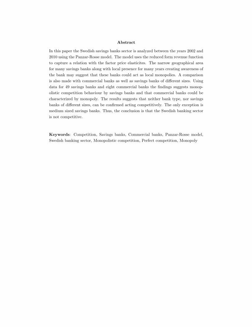
Abstract
In this paper the Swedish savings banks sector is analyzed between the years 2002 and
2010 using the Panzar-Rosse model. The model uses the reduced form revenue function
to capture a relation with the factor price elasticites. The narrow geographical area
for many savings banks along with local presence for many years creating awareness of
the bank may suggest that these banks could act as local monopolies. A comparison
is also made with commercial banks as well as savings banks of different sizes. Using
data for 49 savings banks and eight commercial banks the findings suggests monop-
olistic competition behaviour by savings banks and that commercial banks could be
characterized by monopoly. The results suggests that neither bank type, nor savings
banks of different sizes, can be confirmed acting competitively. The only exception is
medium sized savings banks. Thus, the conclusion is that the Swedish banking sector
is not competitive.
Keywords: Competition, Savings banks, Commercial banks, Panzar-Rosse model,
Swedish banking sector, Monopolistic competition, Perfect competition, Monopoly

Acknowledgements
First and foremost I would like to express my sincere thanks and gratitude to my
supervisor Thomas Aronsson for his guidance, support, comments and patience before
and throughout the writing process. Without his help this thesis would not have been
written.
A thanks also to all savings banks who provided data to the study. The Swedish postal
service has seen a large increase in revenues during this period.
Furthermore, I owe gratitude to Sherrill Shaffer for his time and help.
A special thanks is sent to the kind people in the front desk of the Swedish Companies
Registration Office (Bolagsverket) who not only provided help with computers, but
also fetched several cups of well needed coffee.
Audere Est Facere
Andreas Vigren
Contents
1 Introduction 5
1.1 The Swedish banking sector . . . . . . . . . . . . . . . . . . . . . . . . . . . 6
1.2 Previous studies . . . . . . . . . . . . . . . . . . . . . . . . . . . . . . . . . 8
1.3 Purpose . . . . . . . . . . . . . . . . . . . . . . . . . . . . . . . . . . . . . . 10
1.4 Research question . . . . . . . . . . . . . . . . . . . . . . . . . . . . . . . . . 11
2 Theoretical Framework 11
2.1 The Panzar-Rosse model . . . . . . . . . . . . . . . . . . . . . . . . . . . . . 12
2.2 Empirical model . . . . . . . . . . . . . . . . . . . . . . . . . . . . . . . . . 19
3 Empirical Framework 20
3.1 Data . . . . . . . . . . . . . . . . . . . . . . . . . . . . . . . . . . . . . . . . 20
3.2 Model . . . . . . . . . . . . . . . . . . . . . . . . . . . . . . . . . . . . . . . 22
4 Results 25
5 Conclusion 29
References 32
Appendix A List of banks 34
Appendix B Econometric appendix 35
B.1 Correlation matrices and descriptive statistics . . . . . . . . . . . . . . . . . 35
B.2 Long-run equilibrium (ROA) test . . . . . . . . . . . . . . . . . . . . . . . . 37
B.3 Estimates including Nordea . . . . . . . . . . . . . . . . . . . . . . . . . . . 38
Appendix C Mathematical appendix 39
C.1 Monopolistic competition (section 2.1.2) . . . . . . . . . . . . . . . . . . . . 39
C.2 Perfect competition (section 2.1.3) . . . . . . . . . . . . . . . . . . . . . . . 40
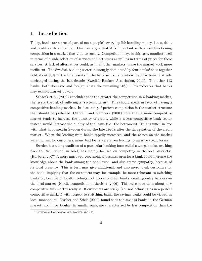
1 Introduction
Today, banks are a crucial part of most people’s everyday life handling money, loans, debit
and credit cards and so on. One can argue that it is important with a well functioning
competition in a market that vital to society. Competition may, in this case, manifest itself
in terms of a wide selection of services and activities as well as in terms of prices for these
services. A lack of alternatives could, as in all other markets, make the market work more
inefficient. The Swedish banking sector is strongly dominated by four banks1 that together
hold about 80% of the total assets in the bank sector, a position that has been relatively
unchanged during the last decade (Swedish Bankers Association, 2011). The other 113
banks, both domestic and foreign, share the remaining 20%. This indicates that banks
may exhibit market power.
Schaeck et al. (2009) concludes that the greater the competition in a banking market,
the less is the risk of suffering a “systemic crisis”. This should speak in favor of having a
competitive banking market. In discussing if perfect competition is the market structure
that should be preferred, Cetorelli and Gambera (2001) note that a more competitive
market tends to increase the quantity of credit, while a a less competitive bank sector
instead would increase the quality of the loans (i.e. the borrowers). This is much in line
with what happened in Sweden during the late 1980’s after the deregulation of the credit
market. When the lending from banks rapidly increased, and the actors on the market
were fighting for customers, many bad loans were given leading to massive credit losses.
Sweden has a long tradition of a particular banking form called savings banks, reaching
back to 1820, which, in brief, has mainly focused on competing in the local districts’.
(Korberg, 2007) A more narrowed geographical business area for a bank could increase the
knowledge about the bank among the population, and also create sympathy, because of
its local presence. This is turn may give additional, and also more loyal, customers for
the bank, implying that the customers may, for example, be more reluctant to switching
banks or, because of loyalty feelings, not choosing other banks, creating entry barriers on
the local market (Nordic competition authorities, 2006). This raises questions about how
competitive this market really is. If customers are sticky (i.e. not behaving as in a perfect
competitive market) with respect to switching bank, the savings banks could be viewed as
local monopolies. Gischer and Stiele (2009) found that the savings banks in the German
market, and in particular the smaller ones, are characterized by less competition than the
1Swedbank, Handelsbanken, Nordea and SEB
5
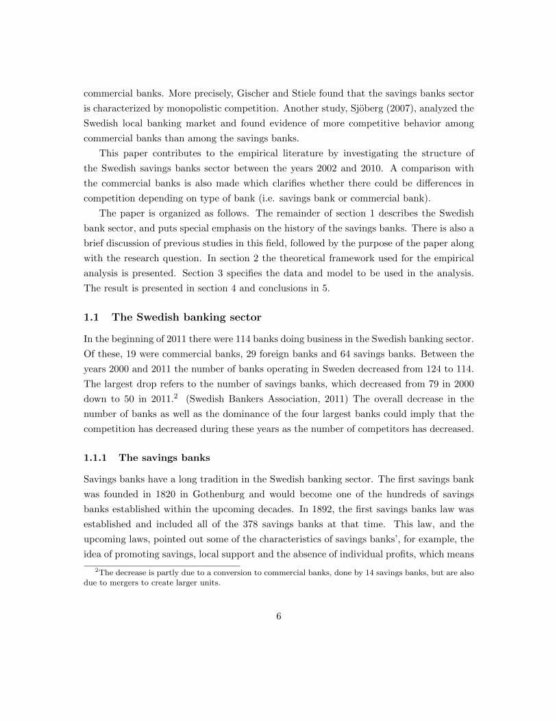
commercial banks. More precisely, Gischer and Stiele found that the savings banks sector
is characterized by monopolistic competition. Another study, Sjoberg (2007), analyzed the
Swedish local banking market and found evidence of more competitive behavior among
commercial banks than among the savings banks.
This paper contributes to the empirical literature by investigating the structure of
the Swedish savings banks sector between the years 2002 and 2010. A comparison with
the commercial banks is also made which clarifies whether there could be differences in
competition depending on type of bank (i.e. savings bank or commercial bank).
The paper is organized as follows. The remainder of section 1 describes the Swedish
bank sector, and puts special emphasis on the history of the savings banks. There is also a
brief discussion of previous studies in this field, followed by the purpose of the paper along
with the research question. In section 2 the theoretical framework used for the empirical
analysis is presented. Section 3 specifies the data and model to be used in the analysis.
The result is presented in section 4 and conclusions in 5.
1.1 The Swedish banking sector
In the beginning of 2011 there were 114 banks doing business in the Swedish banking sector.
Of these, 19 were commercial banks, 29 foreign banks and 64 savings banks. Between the
years 2000 and 2011 the number of banks operating in Sweden decreased from 124 to 114.
The largest drop refers to the number of savings banks, which decreased from 79 in 2000
down to 50 in 2011.2 (Swedish Bankers Association, 2011) The overall decrease in the
number of banks as well as the dominance of the four largest banks could imply that the
competition has decreased during these years as the number of competitors has decreased.
1.1.1 The savings banks
Savings banks have a long tradition in the Swedish banking sector. The first savings bank
was founded in 1820 in Gothenburg and would become one of the hundreds of savings
banks established within the upcoming decades. In 1892, the first savings banks law was
established and included all of the 378 savings banks at that time. This law, and the
upcoming laws, pointed out some of the characteristics of savings banks’, for example, the
idea of promoting savings, local support and the absence of individual profits, which means
2The decrease is partly due to a conversion to commercial banks, done by 14 savings banks, but are alsodue to mergers to create larger units.
6
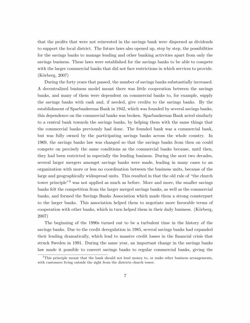
that the profits that were not reinvested in the savings bank were dispersed as dividends
to support the local district. The future laws also opened up, step by step, the possibilities
for the savings banks to manage lending and other banking activities apart from only the
savings business. These laws were established for the savings banks to be able to compete
with the larger commercial banks that did not face restrictions in which services to provide.
(Korberg, 2007)
During the forty years that passed, the number of savings banks substantially increased.
A decentralized business model meant there was little cooperation between the savings
banks, and many of them were dependent on commercial banks to, for example, supply
the savings banks with cash and, if needed, give credits to the savings banks. By the
establishment of Sparbankernas Bank in 1942, which was founded by several savings banks,
this dependence on the commercial banks was broken. Sparbankernas Bank acted similarly
to a central bank towards the savings banks, by helping them with the same things that
the commercial banks previously had done. The founded bank was a commercial bank,
but was fully owned by the participating savings banks across the whole country. In
1969, the savings banks law was changed so that the savings banks from then on could
compete on precisely the same conditions as the commercial banks because, until then,
they had been restricted in especially the lending business. During the next two decades,
several larger mergers amongst savings banks were made, leading in many cases to an
organization with more or less no coordination between the business units, because of the
large and geographically widespread units. This resulted in that the old rule of “the church
tower principle”3 was not applied as much as before. More and more, the smaller savings
banks felt the competition from the larger merged savings banks, as well as the commercial
banks, and formed the Savings Banks Association which made them a strong counterpart
to the larger banks. This association helped them to negotiate more favorable terms of
cooperation with other banks, which in turn helped them in their daily business. (Korberg,
2007)
The beginning of the 1990s turned out to be a turbulent time in the history of the
savings banks. Due to the credit deregulation in 1985, several savings banks had expanded
their lending dramatically, which lead to massive credit losses in the financial crisis that
struck Sweden in 1991. During the same year, an important change in the savings banks
law made it possible to convert savings banks to regular commercial banks, giving the
3This principle meant that the bank should not lend money to, or make other business arrangements,with customers living outside the sight from the districts church tower.
7
possibility to inject capital from outside sources. This possibility had been impossible for
the savings banks, which until then had only been able to rely on the previous profits
of the banks. The change made it possible for eleven savings banks to merge into one
commercial bank, resulting in the publicly listed Sparbanken Sverige AB. This new bank
was formally a public commercial bank, but was to a large extent owned by the savings
banks foundations4. A savings banks foundation are, and was, created when a savings
bank converted to become a commercial bank, and owned the shares in the newly created
commercial bank. The foundations have similar characteristics to the savings banks, which
means that the new commercial banks created by the new law still acted upon the values of
the savings banks. A similar merger as the one creating Sparbanken Sverige was made by
the Foreningsbanks’, creating Foreningsbanken AB, which until then had been a corporate
bank for the past 80 years. In 1997, Sparbanken Sverige and Foreningsbanken merged,
creating one of the largest banks in Sweden, Foreningssparbanken, which later changed its
name to Swedbank. (Korberg, 2007)
Today, the majority of the savings banks have a strong connection to Swedbank through
an intimate cooperation agreement where they share, for example, technological platforms
and possibilities for customers in the savings banks and Swedbank to use each other’s
branches for banking services. However, all savings banks that did not participate in the
merger to Sparbanken Sverige are, regardless of if it is a “pure” savings bank or a converted
commercial bank, still independent firms. A list of these banks are provided in appendix
A.
1.2 Previous studies
Today, a vast literature about the competition in the banking sector exists and is based
on different statistical methods. In this section, a selection of studies is discussed focusing
mainly on the Swedish banking sector, but also studies from Germany as the savings banks
have a strong position there.
Vesala (1995) uses the Panzar-Rosse model to investigate competition in the Finnish
banking sector. In brief, the Panzar-Rosse model tries to capture the relationship between
factor price elasticities and the reduced form revenue function at the firm level. This makes
it possible to test whether firms behave as monopolists, monopolistic competitors or in
accordance with perfect competition. A more thorough discussion of this model is provided
4Sparbanksstiftelserna
8
in section 2.1. Vesala conclude that the banks behave in a monopolistic competitive way,
which is a common result from the Panzar-Rosse model (see, for example, table 1)
Schaeck et al. (2009) also applied the Panzar-Rosse model, investigating the relationship
between competition in the banking sector and financial crises for 45 countries during the
years 1980 and 2005. The general findings were monopolistic competition, but the results
vary over countries. Schaeck et al. concludes that concentration cannot proxy competition,
probably due to that competition is a local issue and that the concentration measures do not
capture local competition as they often are conducted at national levels with aggregated
data. The authors estimates a H-statistic consistent with monopolistic competition in
Sweden, and a concentrate ratio of 0.98 based on the three largest banks.
Carbo et al. (2009) applied a number of different approaches to measure competition
in the bank sector in 14 European countries, including Sweden. The approaches used are
the net interest margin to total assets, Lerner Index, Ratio of bank net income to the
value of total assets, Panzar-Rosse model and also the Hirschman-Herfindahl index. The
findings were that the measures are only weakly positively related to each other, meaning
that they probably do not measure the same thing. However, any conclusions about the
Panzar-Rosse model and its fitness to similar methods are not drawn. The authors do,
however, conclude that amongst the four other measures the Lerner index and Returns on
assets are more preferred in measuring overall banking activity. In the study, the Swedish
banking sector was found to be a monopolistic competitive.
In analyzing the competition of the banking sector in the EU, Bikker and Haaf (2002)
found strong evidence for monopolistic competition in most markets, including Sweden,
when using the Panzar-Rosse methodology. Estimations were also conducted at small-
medium- and large bank sizes where the findings were that the degree of competition
declined with the size of the bank. However, this was not true in the Swedish market
where the medium-sized banks had the weakest competition measure.
Turning to the savings banks specifically there is a limited number of studies performed
in the Nordic countries. Sjoberg (2007) found that the Swedish savings banks do not act
in a perfectly competitive market, but not in a “Cournot conduct” either. Sjoberg also
concludes that the competition between savings banks was less than amongst commercial
banks.
In the German savings banks sector both Hempell (2002) and Gischer and Stiele (2009)
found evidence of monopolistic competition using the Panzar-Rosse approach. In their
analysis of the German savings bank Sparkassen the authors also found that smaller savings
9
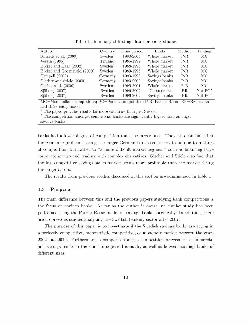
Table 1: Summary of findings from previous studies
Author Country Time period Banks Method FindingSchaeck et al. (2009) Sweden1 1980-2005 Whole market P-R MCVesala (1995) Finland 1985-1992 Whole market P-R MCBikker and Haaf (2002) Sweden1 1988-1998 Whole market P-R MCBikker and Groeneveld (2000) Sweden1 1989-1996 Whole market P-R MCHempell (2002) Germany 1993-1998 Savings banks P-R MCGischer and Stiele (2009) Germany 1993-2002 Savings banks P-R MCCarbo et al. (2009) Sweden1 1995-2001 Whole market P-R MCSjoberg (2007) Sweden 1996-2002 Commercial BR Not PC2
Sjoberg (2007) Sweden 1996-2002 Savings banks BR Not PC2
MC=Monopolistic competition; PC=Perfect competition; P-R: Panzar-Rosse; BR=Bresnahanand Reiss entry model1 The paper provides results for more countries than just Sweden2 The competition amongst commercial banks are significantly higher than amongstsavings banks
banks had a lower degree of competition than the larger ones. They also conclude that
the economic problems facing the larger German banks seems not to be due to matters
of competition, but rather to “a more difficult market segment” such as financing large
corporate groups and trading with complex derivatives. Gischer and Stiele also find that
the less competitive savings banks market seems more profitable than the market facing
the larger actors.
The results from previous studies discussed in this section are summarized in table 1
1.3 Purpose
The main difference between this and the previous papers studying bank competitions is
the focus on savings banks. As far as the author is aware, no similar study has been
performed using the Panzar-Rosse model on savings banks specifically. In addition, there
are no previous studies analyzing the Swedish banking sector after 2007.
The purpose of this paper is to investigate if the Swedish savings banks are acting in
a perfectly competitive, monopolistic competitive, or monopoly market between the years
2002 and 2010. Furthermore, a comparison of the competition between the commercial
and savings banks in the same time period is made, as well as between savings banks of
different sizes.
10
1.4 Research question
Is the Swedish savings banks industry acting competitive, or is it rather characterized by
monopolistic competition or behaving as local monopolies? In addition, are there any
differences compared to the competition amongst commercial banks or savings banks of
different sizes?
2 Theoretical Framework
In measuring competition several methods are used in the literature, and the most fre-
quently used methods will be described below. A popular method is the Bresnahan-Lau
model. By defining demand- and supply functions for a product or market one can es-
timate, assuming that firms are not price takers, a markup (λ) from the price equation
(obtained from the supply function), where λ ∈ (0, 1). A value zero implies that the
market is characterized by perfect competition, whilst a value of one denotes a monopoly
market.(Bresnahan, 1982) (Lau, 1982) As the Bresnahan-Lau model requires data at the
market level, it is hard to apply the model on the banking market due to difficulties to
find appropriate explanatory variables in the demand and supply functions, especially the
price variable.
The Boone indicator has recently been applied (see e.g. van Leuvensteijn et al. (2010)
and van Leuvensteijn et al. (2011)). The model is built on the assumption that a more
efficient firm (firms with lower marginal cost) will be more competitive than a less effi-
cient one. Thus, by analyzing market shares and marginal costs, an indicator is obtained
measuring the degree of competition. The indicator has a more negative value (larger in
absolute terms) the more competitive a market is.
Another approach is typically referred to as the Panzar-Rosse model. Panzar and Rosse
(1987) developed a theoretical model which builds upon the elasticities of the firms income
with respect to factor prices, and that the competition could be tested from those. A
thorough explanation of this model is given in section 2.1. A major advantage of the
Panzar-Rosse model is that it does not require data on the market level, but instead uses
firm level data, which is easier to find. Also, it is possible to distinguish between more
forms of imperfect competition than just monopoly (compare with, e.g., the Bresnahan-Lau
model). Some disadvantages is that a banks annual reports might report data from more
than one market (e.g. other countries) which must be taken into consideration. Also, larger
11
banks most often make larger profits etc. which can cause problems in the estimation. A
solution to this is to divide the sample into different classes of size. In addition, since the
Panzar-Rosse model assumes that the sample is in long-run equilibrium the results from a
non-long-run equilibrium sample may cause spurious and unreliable results.5 Although the
Panzar-Rosse model has disadvantages, it will be used in this paper as it fits the banking
market well and are widely applied in academical literature.
2.1 The Panzar-Rosse model
John C. Panzar and James N. Rosse introduced a test for imperfect market structures,
which has been widely used when analyzing the competitiveness of different markets. In
brief, the model uses comparative statics from the firms reduced form revenue function, and
thereafter the sum of the factor price elasticities to determine the degree of competition.
(Panzar and Rosse, 1987) The model is based on the assumptions that the firms in the
sample are profit maximizing, that the sample must be in a long-run equilibrium, and
that the average cost curve is convex with respect to price and quantity. All of these
assumptions are assumed to be fulfilled. The presentation of the model given in section
2.1 mainly follows the articles of Panzar and Rosse (1977) and Panzar and Rosse (1987),
if nothing else is referenced. This theoretical framework will be the foundation of the
empirical model presented in section 2.2. The model will from now on also be referred to
as the PR-model.
2.1.1 The monopoly case
Consider a monopoly firm. If y is a vector of output variables affecting firm revenue, and z
a vector of q exogenous variables shifting the revenue function of the curve, the sole firms
revenue function can be described as
R = R(y, z) (2.1)
The firm’s cost is either directly, or indirectly, connected to y resulting in a cost function
C = C(y, w, t) (2.2)
5A test for long-run equilibrium is available through Shaffer (1982) and is presented in section 2.2.1
12
where w is a vector of factor prices and t a vector of variables shifting the firms cost
function. It is also possible for z and t to have common variables. Profits of the firm can
be expressed as
π = R− C = π(y, z, w, t) (2.3)
Define y0 = arg maxyπ(y, z, w, t) and y1 = arg maxyπ(y, z, (1 + h)w, t) where the scalar
h > 0. Also define R0 = R(y0, z) ≡ R∗(z, w, t) and R1 = R(y1, z) ≡ R∗[z, (1 + h)w, t],
where R∗ is the reduced form revenue function of the firm. By using equation (2.3) and that
the cost function is homogenous of degree one, the following is true by profit maximization
R1 − (1 + h)C(y1, w, t) > R0 − (1 + h)C(y0, w, t) (2.4)
and
R0 − C(y0, w, t) > R1 − C(y1, w, t) (2.5)
Multiplying (2.5) with (1 + h)
(1 + h)[R0 − C(y0, w, t)] > (1 + h)[R1 − C(y1, w, t)] (2.6)
and adding (2.6) to (2.4) gives
(1 + h)[R0 − C(y0, w, t)]− (1 + h)[R1 − C(y1, w, t)]
+R1 − (1 + h)C(y1, w, t)−R0 + (1 + h)C(y0, w, t) > 0
− h(R1 −R0) > 0 (2.7)
Dividing (2.7) with h2 gives
R1 −R0
h=R∗[z, (1 + h)w, t]−R∗(z, w, t)
h6 0 (2.8)
Equation (2.8) shows that an equiproportional cost increase results in a decrease in the rev-
enues of the firm. Assuming that the firms reduced form revenue functions is differentiable,
taking the limit of h and dividing with R∗
Ψ∗ ≡i∑
i=1
∂R∗
∂wi
wi
R∗ 6 0 (2.9)
13
which gives the sum of factor price elasticities of the reduced form revenue function. Equa-
tion (2.9) shows that the sum of these elasticities must be nonpositive in the case of a
monopoly firm.
2.1.2 Monopolistic competition
In the case of differentiated products across various firms, the monopolistic competition
case is a possible market imperfection. Panzar and Rosse argue, with a discussion about
the work by Chamberlin (1962) and the Chamberlin equilibrium, that
“Each firm, viewed in isolation, would, in both theories6, behave exactly as a monopoly would,
and its actions would satisfy all the conditions of profit maximization. Nevertheless it may be hoped
that by examining the effects of changes in exogenous variables the “hidden” forces of Chamberlin’s
“group equilibrium” condition may come into focus” - (Panzar and Rosse, 1987, p. 448-449)
The analysis is thus based on how the single acts in a long-run equilibrium, when prices and
number of firms active on the market have adjusted. A way to distinguish the monopolistic
competition case from perfect competition is desirable, and also possible to do by analyzing
the elasticity of factor prices derived later in this section. The monopolistic competition
concept used here could be called “The long-run monopolistic competition” or ‘Chamber-
linian Monopolistic Competition” and is a long-run equilibrium where the number of firms
is endogenous.
By using comparative statics and defining R(y, n, z) = yP (y, n, z), where n is the
number of firms , the monopolistic competition case is defined by equation (2.10) and
(2.11) and describes the long-run equilibrium values y∗ and n∗, treating the other variables
as exogenous.
Ry(y∗, n∗, z)− Cy(y∗, w, t) = 0 (2.10)
R(y∗, n∗, z)− C(y∗, w, t) = 0 (2.11)
In order to derive an expression for the factor price elasticities, using that R(y∗, n∗, z) =
R∗(z, w, t) from section 2.1.1 and the chain rule, differentiating (2.11) gives
∂R∗
∂wi= Cy
∂y∗
∂wi+∂C
∂wi= Cy
∂y∗
∂wi+ x∗i (2.12)
where x∗i is the optimal quantity of production factor i, following Shepard’s lemma. Multi-
6The pure monopoly and the pure competition (authors note)
14
plying by (wi/R∗) and summing over equation (2.12)
Ψ∗ =
i∑i=1
wi
R∗∂R∗
∂wi
=Cy
R∗
i∑i=1
wi∂y∗
∂wi+
C
R∗ (2.13)
Thus, an expression for the factor price elasticities is defined. ∂y∗/∂wi is obtained by
totally differentiating (2.10) and (2.11) with respect to y∗, n∗ and wi, and solving using
Cramer’s rule7∂y∗
∂wi=Rn(∂x∗i /∂y)−Rynx
∗i
D∗ (2.14)
where D∗ = (Ryy − Cyy)Rn > 0 from appendix C.1. Substituting (2.11) and (2.14) into
equation(2.13) gives
Ψ∗ =Cy[Rn
∑wi(∂x
∗i /∂y)−Ryn
∑wix
∗i ]
R∗D∗ + 1
As x∗i represents the cost minimizing input factor i, a change in this when the output level
(y) changes should equal marginal cost if multiplied with wi.
i∑i=1
wi(∂x∗i /∂y) =
∂C
∂y= Cy
From this, and using that∑i
i=1wix∗i = C, it follows that
Ψ∗ = 1 +Cy[RnCy −RynC]
R∗D∗
Again using (2.10) and (2.11)
Ψ∗ = 1 +Ry[RnRy −RRyn]
R∗D∗ (2.15)
By using the inverse demand function and the fact that R = Py, the bracketed term
7A complete derivation of the steps leading to equation 2.14 is provided in appendix C.1
15
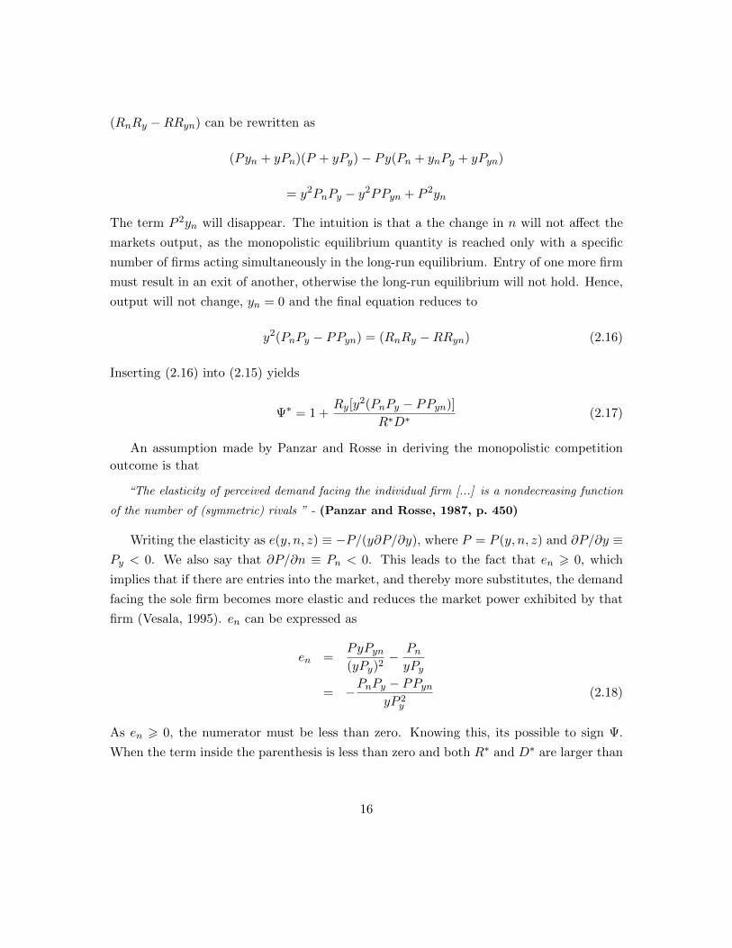
(RnRy −RRyn) can be rewritten as
(Pyn + yPn)(P + yPy)− Py(Pn + ynPy + yPyn)
= y2PnPy − y2PPyn + P 2yn
The term P 2yn will disappear. The intuition is that a the change in n will not affect the
markets output, as the monopolistic equilibrium quantity is reached only with a specific
number of firms acting simultaneously in the long-run equilibrium. Entry of one more firm
must result in an exit of another, otherwise the long-run equilibrium will not hold. Hence,
output will not change, yn = 0 and the final equation reduces to
y2(PnPy − PPyn) = (RnRy −RRyn) (2.16)
Inserting (2.16) into (2.15) yields
Ψ∗ = 1 +Ry[y2(PnPy − PPyn)]
R∗D∗ (2.17)
An assumption made by Panzar and Rosse in deriving the monopolistic competition
outcome is that
“The elasticity of perceived demand facing the individual firm [...] is a nondecreasing function
of the number of (symmetric) rivals ” - (Panzar and Rosse, 1987, p. 450)
Writing the elasticity as e(y, n, z) ≡ −P/(y∂P/∂y), where P = P (y, n, z) and ∂P/∂y ≡Py < 0. We also say that ∂P/∂n ≡ Pn < 0. This leads to the fact that en > 0, which
implies that if there are entries into the market, and thereby more substitutes, the demand
facing the sole firm becomes more elastic and reduces the market power exhibited by that
firm (Vesala, 1995). en can be expressed as
en =PyPyn
(yPy)2− Pn
yPy
= −PnPy − PPyn
yP 2y
(2.18)
As en > 0, the numerator must be less than zero. Knowing this, its possible to sign Ψ.
When the term inside the parenthesis is less than zero and both R∗ and D∗ are larger than
16
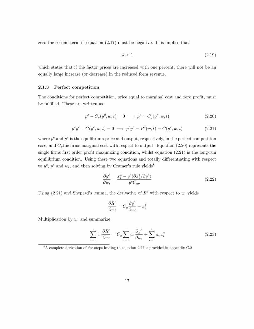
zero the second term in equation (2.17) must be negative. This implies that
Ψ < 1 (2.19)
which states that if the factor prices are increased with one percent, there will not be an
equally large increase (or decrease) in the reduced form revenue.
2.1.3 Perfect competition
The conditions for perfect competition, price equal to marginal cost and zero profit, must
be fulfilled. These are written as
pc − Cy(yc, w, t) = 0 =⇒ pc = Cy(yc, w, t) (2.20)
pcyc − C(yc, w, t) = 0 =⇒ pcyc = Rc(w, t) = C(yc, w, t) (2.21)
where pc and yc is the equilibrium price and output, respectively, in the perfect competition
case, and Cythe firms marginal cost with respect to output. Equation (2.20) represents the
single firms first order profit maximizing condition, whilst equation (2.21) is the long-run
equilibrium condition. Using these two equations and totally differentiating with respect
to yc, pc and wi, and then solving by Cramer’s rule yields8
∂yc
∂wi=x∗i − yc(∂x∗i /∂yc)
ycCyy(2.22)
Using (2.21) and Shepard’s lemma, the derivative of Rc with respect to wi yields
∂Rc
∂wi= Cy
∂yc
∂wi+ x∗i
Multiplication by wi and summarize
i∑i=1
wi∂Rc
∂wi= Cy
i∑i=1
wi∂yc
∂wi+
i∑i=1
wix∗i (2.23)
8A complete derivation of the steps leading to equation 2.22 is provided in appendix C.2
17
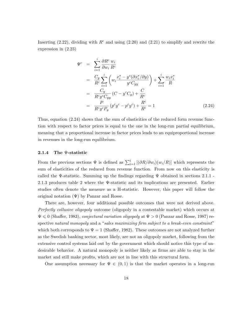
Inserting (2.22), dividing with Rc and using (2.20) and (2.21) to simplify and rewrite the
expression in (2.23)
Ψc =i∑
i=1
∂Rc
∂wi
wi
Rc
=Cy
Rc
i∑i=1
(wix∗i − yc(∂x∗i /∂y)
ycCyy
)+
i∑i=1
wix∗i
R
=Cy
RcycCyy(C − ycCy) +
C
Rc
=P
RcycPy(pcyc − pcyc) +
Rc
Rc= 1 (2.24)
Thus, equation (2.24) shows that the sum of elasticities of the reduced form revenue func-
tion with respect to factor prices is equal to the one in the long-run partial equilibrium,
meaning that a proportional increase in factor prices leads to an equiproportional increase
in revenues in the long-run equilibrium.
2.1.4 The Ψ-statistic
From the previous sections Ψ is defined as∑i
i=1 [(∂R/∂wi)(wi/R)] which represents the
sum of elasticities of the reduced from revenue function. From now on this elasticity is
called the Ψ-statistic. Summing up the findings regarding Ψ obtained in sections 2.1.1 -
2.1.3 produces table 2 where the Ψ-statistic and its implications are presented. Earlier
studies often denote the measure as a H-statistic. However, this paper will follow the
original notation (Ψ) by Panzar and Rosse.
There are, however, four additional possible outcomes that were not derived above.
Perfectly collusive oligopoly outcome (oligopoly in a contestable market) which occurs at
Ψ 6 0 (Shaffer, 1983), conjectural variation oligopoly at Ψ > 0 (Panzar and Rosse, 1987) re-
spective natural monopoly and a “sales maximizing firm subject to a break-even constraint”
which both corresponds to Ψ = 1 (Shaffer, 1982). These outcomes are not analyzed further
as the Swedish banking sector, most likely, are not an oligopoly market, following from the
extensive control systems laid out by the government which should notice this type of un-
desirable behavior. A natural monopoly is neither likely as firms are able to stay in the
market and still make profits, which are not in line with this structural form.
One assumption necessary for Ψ ∈ (0, 1) is that the market operates in a long-run
18
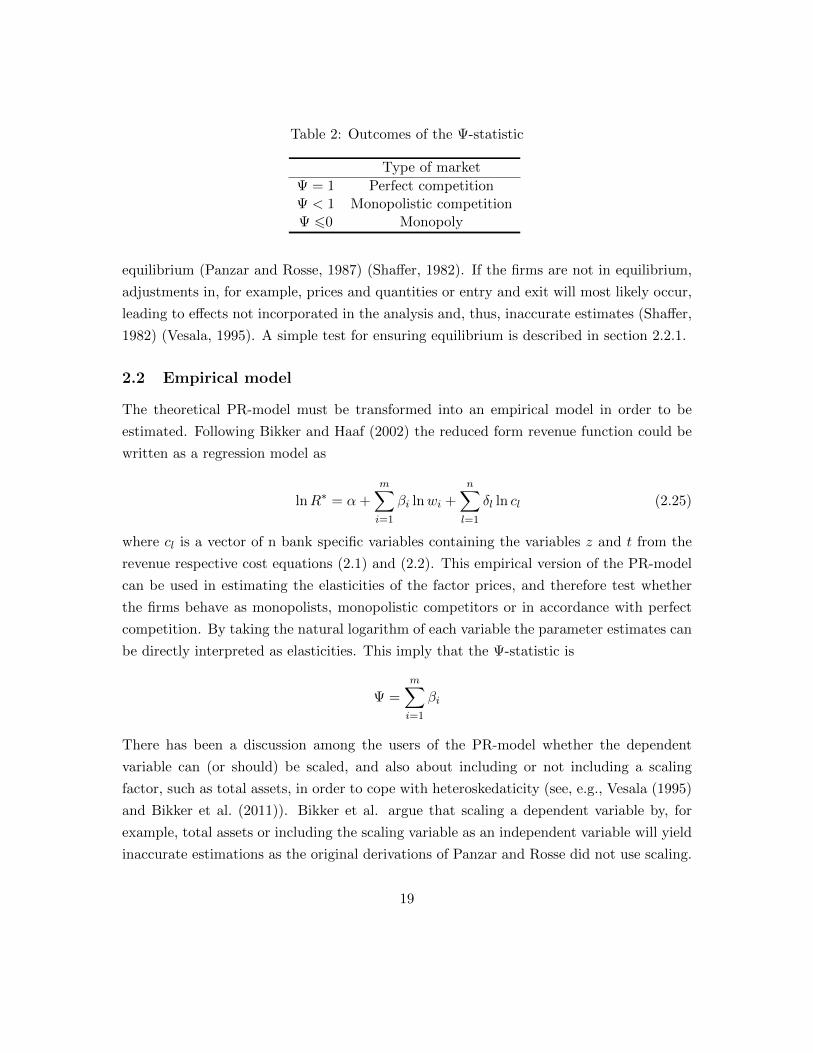
Table 2: Outcomes of the Ψ-statistic
Type of market
Ψ = 1 Perfect competitionΨ < 1 Monopolistic competitionΨ 60 Monopoly
equilibrium (Panzar and Rosse, 1987) (Shaffer, 1982). If the firms are not in equilibrium,
adjustments in, for example, prices and quantities or entry and exit will most likely occur,
leading to effects not incorporated in the analysis and, thus, inaccurate estimates (Shaffer,
1982) (Vesala, 1995). A simple test for ensuring equilibrium is described in section 2.2.1.
2.2 Empirical model
The theoretical PR-model must be transformed into an empirical model in order to be
estimated. Following Bikker and Haaf (2002) the reduced form revenue function could be
written as a regression model as
lnR∗ = α+
m∑i=1
βi lnwi +
n∑l=1
δl ln cl (2.25)
where cl is a vector of n bank specific variables containing the variables z and t from the
revenue respective cost equations (2.1) and (2.2). This empirical version of the PR-model
can be used in estimating the elasticities of the factor prices, and therefore test whether
the firms behave as monopolists, monopolistic competitors or in accordance with perfect
competition. By taking the natural logarithm of each variable the parameter estimates can
be directly interpreted as elasticities. This imply that the Ψ-statistic is
Ψ =
m∑i=1
βi
There has been a discussion among the users of the PR-model whether the dependent
variable can (or should) be scaled, and also about including or not including a scaling
factor, such as total assets, in order to cope with heteroskedaticity (see, e.g., Vesala (1995)
and Bikker et al. (2011)). Bikker et al. argue that scaling a dependent variable by, for
example, total assets or including the scaling variable as an independent variable will yield
inaccurate estimations as the original derivations of Panzar and Rosse did not use scaling.
19
Scaling the dependent variable makes the revenue function become a price function, which
will not work in the estimations of the Ψ-statistic. (Bikker et al., 2011). In this study, the
dependent variable will not be scaled, nor will any separate scaling factor, such as total
assets, be included which is in line with the discussion of Bikker et al.
2.2.1 Test for long-run equilibrium
As was described in section 2.1.4, the sample used in estimating the Ψ-statistic needs to be
in a long-run equilibrium. A widely used method (see (Nathan and Neave, 1989), (Claessens
and Laeven, 2004) or (Gischer and Stiele, 2009)) is the one proposed by (Shaffer, 1982)
where an empirical test for equilibrium is conducted by replacing the dependent variable
with a variable representing rate of return. Shaffer writes
“If the risk level of a bank is unaffected by its input prices within the observed range of prices,
and if all banks in the sample compete in the same capital market, then equilibrium rates of return
should not be statistically correlated with input prices. If, however, the banks are in transition toward
a new equilibrium, then an increase (decrease) in factor prices would show up as a temporary decline
(increase) in the rate of return producing a negative correlation between factor prices and the rate
of return.” - (Shaffer, 1982, p. 230)
Thus, by using returns on assets (ROA) as the dependent variable, an approach adopted
by many other studies, if the ΨROA-statistic sums to zero, and a hypothesis test confirms
equality to zero, the sample is indeed in long-run equilibrium. The statistic is defined as
ΨROA =∑ ∂ROA
∂wi
wi
ROA
3 Empirical Framework
3.1 Data
The data is a strongly balanced panel data set collected from the annual reports of each
bank. The banks included in the sample are shown in appendix A. The time range is 2002 to
2010. The choice of time period is mainly due to that the Swedish Companies Registration
Office (SCRO)9 only keeps digital copies of the annual reports up to ten years, and the
reports for the year 2011 have not been published yet by the majority of banks. The data
is partly also available through Statistics Sweden (SCB), but because of the analysis of
9Bolagsverket
20
savings banks, which often tend to be small and do not report to SCB, this source does not
contain much of the data needed.10 The banks included in the data set are retail banks,
meaning that they offer regular bank services (e.g. mortgage lending and debit- and credit
cards) to the broad public. This is to make sure the market is fairly the same for all banks
in the sample and are therefore excluding niche banks.
The collected data mainly follows the international accounting standard IFRS. Nordea
and ICA Banken reports their results in euro for the whole time period respective since
2009. The yearly average exchange rate EUR/SEK for respective year is used to convert
the numbers into Swedish kronor, which is the currency used in the data set. All monetary
variables are expressed with their real values in 2012 by the consumer price index provided
by SCB.
3.1.1 Exclusion of banks
Unfortunately it is not possible to use data for all savings banks. The main reason is that
15 out of 64 savings banks are missing data due to missing records of annual reports in
the archives of the SCRO. Attempts to contact these banks and receive reports directly
from them have also been made without any success. A full list of which savings banks
not included is provided in appendix A. Although 15 savings banks are missing, it is a
fair assumption that the results of this paper will not be affected significantly and the
estimation process still be valid as there are 49 banks remaining.
In the estimation of competition within commercial banks there is also firms missing.
A list of banks is provided in appendix A. The majority of banks excluded are done so
because their main business area in Sweden are not retail banking but instead have a niche
towards, for example, investment banking or savings11.
The banks included are also acting mainly in the Swedish market, meaning that the
majority of their income originates from Swedish customers, which excludes for example
Danske Bank and DnB Nor which have their largest share of customers in Denmark and
Norway. A consequence of this is that one of the four largest banks acting at the Swedish
market, Nordea, is also excluded. The reason being that the income from the Swedish
market represents about 25% of their total income. Including Nordea could alter the
assumption of banks acting in the same market because of their large involvement in
10The same reasoning holds for other databases, such as Bankscope or OSIRIS11It is important to distinguish between savings banks (the bank type) and banks involved only or mainly
in savings business (for example Avanza Bank or Nordnet Bank)
21

other countries, and therefore also competition with other actors that the other banks in
the sample do not face. For completeness, estimations including Nordea is provided in
appendix B.3. The same reasoning could be applied on especially Swedbank and SEB due
to their activity in the Baltic countries, but also Handelsbanken and its involvement in the
British bank market. These three banks are, however, not excluded because their share of
income from the Swedish market is at least about 70% of their respective total income and
are therefore considered to compete mainly on the Swedish market. As the purpose of this
thesis mainly is to write about the competition of savings banks, the exclusion of Nordea
do not affect the savings banks result, nor the commercial bank results which is obvious
by comparing table 4 and 10.
3.2 Model
There are almost as many different variations of the Panzar-Rosse model as there are
articles. One common factor is, however, the dependent variable, corresponding to the
revenue, which most often is proxied by the total income (TI) of the bank or total interest
income (TII), both collected from the income statement in the annual reports. The reason
for using total income is that banks today have other business areas than just the ones
generating interest income, such as debit card and insurances, and that all of them should
be taken into account. A drawback of using total income is that, for example, losses in a
banks trading activity is included (as well as profits) lending to dramatically lower income
for several savings banks in 2008 and 2009, partly due to the massive drop in the Swedbank
share price. As the main business of banks is leading, using total interest income should also
make a good proxy for the revenue variable. For completeness, both dependent variables
(TI and TII) are regressed in different specifications.
The proxies for factor prices are the funding rate, cost of personnel and capital expen-
diture. These three factor price variables are widely applied when using the Panzar-Rosse
model (see, for example, Gischer and Stiele (2009) and Molyneux et al. (1996)), although
different calculation methods are used. Definitions of the variables are provided in table 3.
Funding rate is included as this is probably the single most important input factor for
the bank, being able to fund lending. The funding is made partly by deposits and also
other sources such as the central bank and a higher value implies that the bank’s cost of
borrowing are higher.
Personnel are a necessary cost for any firm, whether it works through many or few
22

branches. The bank employees could also be viewed as salesmen trying to improve the
income of the bank. The variable is scaled by the number of employees.
Other operating costs refer to all non-personnel costs a bank faces and proxy the phys-
ical cost of capital, and is scaled with total assets. This post includes, among other things,
marketing and IT expenses as well as rent.
Turning to the bank specific variables (cl in equation (2.25)), there is usually variables
included reflecting risk, funding mix, banking behavior and other control variables. In
order to measure risk, equity to total assets (EQ) is included. A higher equity ratio usually
means the bank is not taking as high risks as with a lower equity, and therefore may not
earn as much income. A higher equity, however, also implies that the bank needs not seek
as much external financing, leading to less interest costs. The sign of this coefficient is
therefore expected to be ambiguous.
Lending towards the public to total assets ratio reflects the banks portfolio composition
and business mix. A higher share of outstanding loans to the public (mainly consumers
and companies) should lead to increased interest revenues, as well as total revenues. The
sign is expected to be positive.
The number of branches operated by the bank is affecting the possibility to be close
to the customer and thereby offering local services and potential additional sales. Many
branches may, in short, lead to a closeness with the community and customers, which
could lead to a larger share of the customers in the area, and thereby also increasing
profits. Branches are, however, associated with higher costs not only for the personnel and
facilities, but also for security and handling cash. The sign of this coefficient is therefore
expected to be ambiguous.
The dependent variable used for determining whether the sample is in long-run equi-
librium is defined as the operating result divided by total assets, plus one to account for
negative operating results.
In addition, regressions will be conducted to analyze if there is any difference in com-
petitive behavior between small, medium sized and large savings banks. Findings from,
for instance, Gischer and Stiele (2009) suggest that smaller savings banks tend to behave
less competitive than larger ones. Thus, this is an interesting aspect to investigate also in
Sweden. The division between different sizes is based on the number of employees where
the 33 and 66 percentile has been used as limits for respective size. The 33 percentile
occurs at 25 employees, and the 66 percentile at 70.
The empirical models run in the regressions for bank i at time t are specified as
23
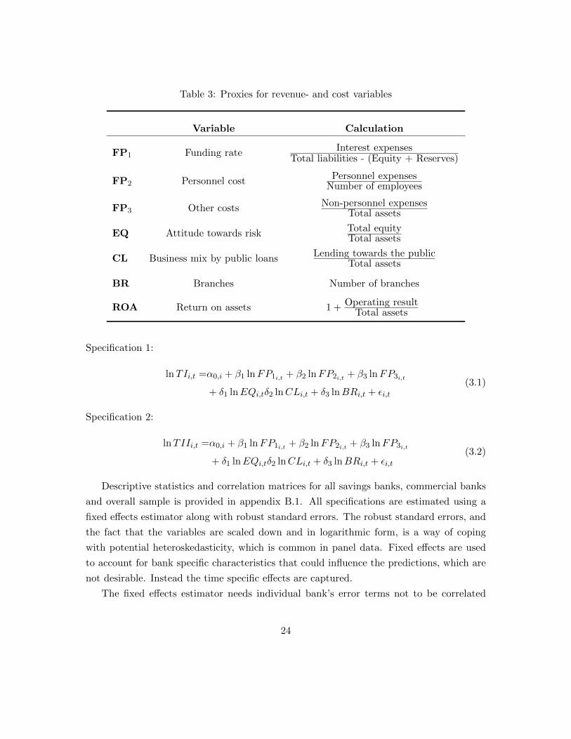
Table 3: Proxies for revenue- and cost variables
Variable Calculation
FP1 Funding rateInterest expenses
Total liabilities - (Equity + Reserves)
FP2 Personnel costPersonnel expenses
Number of employees
FP3 Other costsNon-personnel expenses
Total assets
EQ Attitude towards riskTotal equityTotal assets
CL Business mix by public loansLending towards the public
Total assets
BR Branches Number of branches
ROA Return on assets 1 +Operating result
Total assets
Specification 1:
lnTIi,t =α0,i + β1 lnFP1i,t + β2 lnFP2i,t + β3 lnFP3i,t
+ δ1 lnEQi,tδ2 lnCLi,t + δ3 lnBRi,t + εi,t(3.1)
Specification 2:
lnTIIi,t =α0,i + β1 lnFP1i,t + β2 lnFP2i,t + β3 lnFP3i,t
+ δ1 lnEQi,tδ2 lnCLi,t + δ3 lnBRi,t + εi,t(3.2)
Descriptive statistics and correlation matrices for all savings banks, commercial banks
and overall sample is provided in appendix B.1. All specifications are estimated using a
fixed effects estimator along with robust standard errors. The robust standard errors, and
the fact that the variables are scaled down and in logarithmic form, is a way of coping
with potential heteroskedasticity, which is common in panel data. Fixed effects are used
to account for bank specific characteristics that could influence the predictions, which are
not desirable. Instead the time specific effects are captured.
The fixed effects estimator needs individual bank’s error terms not to be correlated
24
with that of other banks, thus a Hausman test is conducted to every group to determines if
the fixed effects estimator is the appropriate one to use, or if the random effects estimator
should be used instead. All χ2-statistics produced from the Hausman test are significant
at 5%-level or less which confirms the use of the fixed effects estimator. In order to test
whether the obtained Ψ-statistics are statistically distinct from unity (perfect competition)
and/or zero (monopoly), Wald test’s is conducted. Thus, the hypothesis of these tests are
Ψ = 0 and Ψ = 1.
The test for long-run equilibrium is performed by regressing the model
lnROAi,t =α0,i + φ1 lnFP1i,t + φ2 lnFP2i,t + φ3 lnFP3i,t
+ δ1 lnEQi,tδ2 lnCLi,t + δ3 lnBRi,t + εi,t(3.3)
As specification 1 and 2 contain the same independent variables, only one equilibrium
specification is needed. A fixed effects estimation is done with robust standard errors also
for this model. As explained in section 2.2.1, the sum of factor price elasticities in equation
(3.3) should be zero for the models to be in long-run equilibrium, thus
ΨROA = φ1 + φ2 + φ3 = 0 (3.4)
4 Results
The estimation results from specification I and II are provided in table 4 on pages 26
and 27. Applying Wooldridge’s test for serial correlation12 in fixed effects panel data
sets no significant p-values was generated, meaning no serial correlation was found. The
correlation matrices in appendix B.1 show no sign of correlation between variables that
must be corrected for.
The long-run equilibrium test is provided in appendix B.2. All specification’s and
groups yield ΨROA estimates around zero, implying a long-run equilibrium bank sector.
By using a Wald test, the null hypothesis that ΨROA = 0 could not be rejected.
Turning to the main results from the estimations, the banks funding rate (β1) has a
significant effect in all cases, but one, and yields a slightly negative estimate using total
income as dependent variable, but positive if using total interest income. The p-values using
12see Drukker (2003)
25
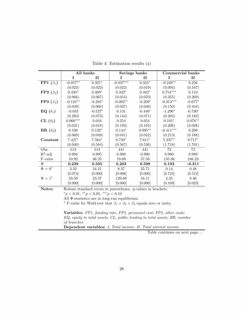
Table 4: Estimation results (a)
All banks Savings banks Commercial banksI II I II I II
FP1 (β1) -0.057∗∗ 0.321∗ -0.037∗∗∗ 0.325∗ -0.248∗∗ 0.256(0.023) (0.023) (0.022) (0.019) (0.094) (0.167)
FP2 (β2) 0.420∗ 0.469∗ 0.332∗ 0.482∗ 0.754∗∗∗ 0.110(0.966) (0.067) (0.054) (0.070) (0.355) (0.269)
FP3 (β3) -0.124∗∗ -0.285∗ -0.092∗∗ -0.209∗ -0.313∗∗∗ -0.677∗
(0.049) (0.060) (0.037) (0.046) (0.150) (0.104)EQ (δ1) -0.035 -0.527∗ 0.131 -0.446∗ -1.296∗ -0.730∗
(0.293) (0.073) (0.144) (0.071) (0.205) (0.182)CL (δ2) 0.060∗∗∗ 0.016 0.254 0.054 0.191∗ 0.078∗∗
(0.031) (0.018) (0.193) (0.165) (0.206) (0.028)BR (δ3) 0.106 0.132∗ 0.144∗ 0.095∗∗ -0.411∗∗∗ 0.208
(0.069) (0.049) (0.041) (0.042) (0.213) (0.168)Constant 7.427∗ 7.564∗ 8.720∗ 7.611∗ 5.237∗∗ 9.717∗
(0.940) (0.584) (0.567) (0.526) (1.718) (1.701)Obs. 513 513 441 441 72 72R2-adj 0.988 0.995 0.980 0.990 0.980 0.989F-value 10.92 46.25 19.69 57.56 135.86 246.23Ψ 0.239 0.505 0.203 0.598 0.193 -0.311Ψ = 01 3.32 24.21 8.37 35.71 0.14 0.48
[0.074] [0.000] [0.006] [0.000] [0.724] [0.512]Ψ = 11 33.50 23.37 129.69 16.11 2.35 8.46
[0.000] [0.000] [0.000] [0.000] [0.169] [0.023]
Notes: Robust standard errors in parentheses. p-values in brackets.∗p < 0.01, ∗∗p < 0.05, ∗∗∗p < 0.10All Ψ-statistics are in long-run equilibrium1 F-value for Wald-test that β1 + β2 + β3 equals zero or unity.
Variables: FP1, funding rate; FP2, personnel cost; FP3, other costs;EQ, equity to total assets; CL, public lending to total assets; BR, numberof branchesDependent variables: I, Total income; II, Total interest income
Table continues on next page. . .
26
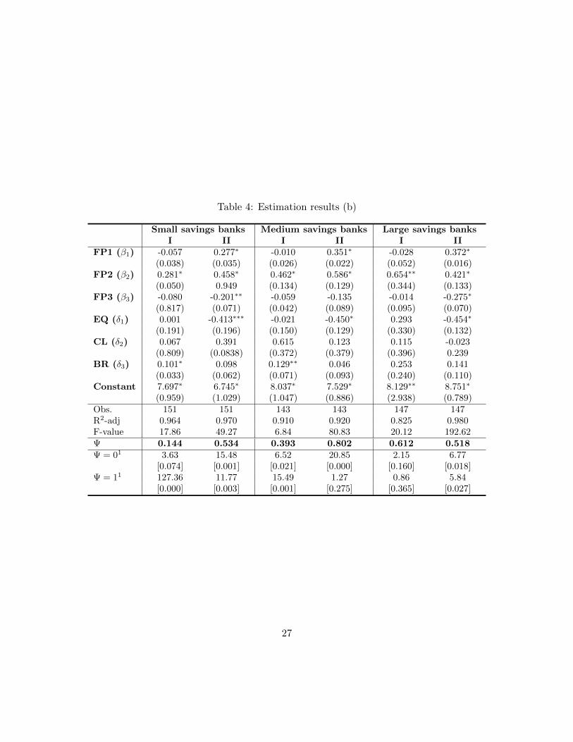
Table 4: Estimation results (b)
Small savings banks Medium savings banks Large savings banksI II I II I II
FP1 (β1) -0.057 0.277∗ -0.010 0.351∗ -0.028 0.372∗
(0.038) (0.035) (0.026) (0.022) (0.052) (0.016)FP2 (β2) 0.281∗ 0.458∗ 0.462∗ 0.586∗ 0.654∗∗ 0.421∗
(0.050) 0.949 (0.134) (0.129) (0.344) (0.133)FP3 (β3) -0.080 -0.201∗∗ -0.059 -0.135 -0.014 -0.275∗
(0.817) (0.071) (0.042) (0.089) (0.095) (0.070)EQ (δ1) 0.001 -0.413∗∗∗ -0.021 -0.450∗ 0.293 -0.454∗
(0.191) (0.196) (0.150) (0.129) (0.330) (0.132)CL (δ2) 0.067 0.391 0.615 0.123 0.115 -0.023
(0.809) (0.0838) (0.372) (0.379) (0.396) 0.239BR (δ3) 0.101∗ 0.098 0.129∗∗ 0.046 0.253 0.141
(0.033) (0.062) (0.071) (0.093) (0.240) (0.110)Constant 7.697∗ 6.745∗ 8.037∗ 7.529∗ 8.129∗∗ 8.751∗
(0.959) (1.029) (1.047) (0.886) (2.938) (0.789)Obs. 151 151 143 143 147 147R2-adj 0.964 0.970 0.910 0.920 0.825 0.980F-value 17.86 49.27 6.84 80.83 20.12 192.62Ψ 0.144 0.534 0.393 0.802 0.612 0.518Ψ = 01 3.63 15.48 6.52 20.85 2.15 6.77
[0.074] [0.001] [0.021] [0.000] [0.160] [0.018]Ψ = 11 127.36 11.77 15.49 1.27 0.86 5.84
[0.000] [0.003] [0.001] [0.275] [0.365] [0.027]
27
total income are above the 10%-level for all regressions run on different sizes. Increasing
the funding of the bank yields higher interest income, but lower total income.
The personnel costs (β2) have a positive effect in both specifications which is significant
mostly at the 1%-level. The personnel as factor price has a positive impact on the sales
of the bank, not only in yielding good interest income but also when it comes to other
business areas, proxied by the total income variable. This variable has the greatest impact
on Ψ and could therefore be regarded as the most important feature of the bank.
The estimated effects of other costs (β3) imply that increasing this post will yield lower
total- and interest income. Being significant mostly at the aggregated regressions (e.g.
including all banks of each type) it implies that increasing costs referring to, for example,
rents or marketing would decrease income.
Turning to the coefficients not associated with the Ψ-statistic there is fairly poor sig-
nificance for each of them depending on specification and group analyzed. The coefficient
taking risk into account (δ1) is in most cases negative or just slightly positive, while the
opposite is true for δ2. For to branches (δ3), an increased number of branches seems to
favor income of the bank as the coefficient is positive for all specifications and groups.
The estimated effects of factor price elasticities give Ψ-statistics that mostly are con-
sistent with monopolistic competition. The one exception is for commercial banks where
using total interest income as dependent variable yields a negative Ψ. Applying Wald test’s
on each statistic, in order to determine if the statistics are different from zero and/or unity,
confirms the conclusion of monopolistic competition for all banks, all savings banks and
small savings banks. This is also true using specification I for medium- and specification
II for large savings banks. Applying the Wald test on specification I for large savings
banks and commercial banks, neither hypothesis of Ψ = 0 or Ψ = 1 can be rejected im-
plying that the structure can not be statistically confirmed by the Ψ-statistic. Looking at
medium savings bank, the hypothesis of perfect competition can not be rejected. Turning
to specification II for commercial banks the unity Wald test can be rejected, but not the
monopoly hypothesis, which is consistent with the negative value of Ψ. Thus, commercial
banks could, using interest income as dependent variable, be characterized by monopoly
behavior.
In appendix B.3 estimates including the commercial bank Nordea is made. The results
show that the estimates of the Ψ-statistics does not differ very much from the ones obtained
by excluding the bank. The sign of the parameter estimates do not differ much (with
exception of the one corresponding to the BR variable, which changes sign), nor does the
28
level of significance for each coefficient.
One explanation of the low significance levels when estimating the model based on
data for the commercial banks, and savings banks of different sizes, are the small number
of observations. In the case of commercial banks a relaxation of the restriction only to
include retail banks could be made, which would increase the number of participating
banks a bit.
5 Conclusion
The purpose of this paper is to study the Swedish savings banks sector and determine if it
is characterized by perfect competition. Earlier studies suggest that the Swedish banking
sector as a whole is acting in a monopolistic competitive manner, and that this also holds
for the savings banks specifically. The analysis is made with the Panzar-Rosse model, which
has been widely applied amongst the academic literature when analyzing bank competition.
The panel data set, obtained from the annual reports of each bank, contains 49 savings
banks and 8 commercial banks. The time period stretches from year 2002 to 2010. Using
a fixed effects model with robust standard errors the estimation results, provided in table
4, are obtained. The dependent variables used are total income of the bank, and total
interest income.
The conclusion is that the Swedish savings banks acts in a monopolistic competitive
manner. The same result holds for the whole Swedish banking sector, whilst the commercial
banks appear to act as monopolists. Thus, there is no evidence of a perfectly competitive
behavior in the Swedish banking sector. The exception is medium sized savings banks
where the hypothesis of perfect competition cannot be rejected. The same is true for large
savings banks where neither this hypothesis, nor the one of monopoly, can be rejected. It
also appears as the savings banks are acting more competitive than the commercial banks.
Despite these results, the estimates for savings banks of different sizes should be inter-
preted carefully as few of the coefficients are statistically significant, and the sample sizes
are fairly small. The sample size argument is also applicable on the commercial banks,
but with the assumptions made to only include retail banks there is no more banks to
include. The over all test and test for all savings banks are, however, most often significant
at 10%-level, probably because they contain a larger sample. Relaxing the assumption of
retail banks will allow more banks to be analyzed, but also raise questions if the banks
are acting in the same market. Although Sweden has a large banking sector, four major
29
players hold the majority of the assets, all of which are commercial banks. This might
justify the low Ψ-statistic estimated for these banks. An interesting aspect of this would
be to analyze the four major banks specifically, as one might suspect that the monopolic
behavior can be tracked to them alone.
The findings of monopolistic competition in the whole banking sector are much in
line with previous studies performed on the Swedish banking sector. See, for example,
Bikker and Groeneveld (2000), Bikker and Haaf (2002) and Carbo et al. (2009) which all
find this with the Panzar-Rosse model, or Sjoberg (2007) who concludes that the local
banking market is not characterized by perfect competition. A comparison of the results
for savings banks with previous studies is not possible to do for the Swedish market as
the Panzar-Rosse model has not yet been applied on the Swedish savings banks sector
by other studies. However, studies performed in the German market are also concluding
monopolistic competition in the savings banks sector (see Gischer and Stiele (2009) and
Hempell (2002)). Hempell (2002) found that the savings banks are less competitive than
commercial banks, which is not the finding in this paper. Also, Gischer and Stiele (2009)
find that the Ψ-statistic is larger for larger savings banks when using total interest income
as dependent variable, which is not entirely the findings in this paper.
Year-to-year estimates for the Ψ-statistics would have been interesting in order to see
the development in competition for every year in the Swedish banking sector. Unfortunately
the number of observations corresponding to each year makes it hard to obtain significant
parameter estimates and valid models for these regressions, especially for the commercial
banks but also for the savings banks. At the same time it is hard to obtain data for more
banks, as the Swedish bank market is relatively small why another approach than the
Panzar-Rosse, or a restated econometric model, might be appropriate.
To summarize, the Swedish savings banks appear to act as monopolistic competitors to
one another, which means they exhibit some market power. They should also, according to
the theory of monopolistic competition, have heterogenous products, which seems plausible
as all banks offer similar products (e.g. loans, cards etc.), but differ in specifics such as
prices, contents or terms. Monopolistic competition also implies that customers are not as
sensitive to price changes as under a competitive market, which leads to higher prices. This,
and the potential monopoly situation among commercial banks, could set a foundation to
analyze the banks mortgage rates, and analyze if the market power exhibited by banks is
exploited to set too high rates. The local presence of savings banks might protect them
to some extent from the four large commercial banks that dominates the banking market
30
because of the possibly quite small local market. The large dependence on Internet and
phone banking does, however, allow commercial banks to act on markets that may not be
profitable to establish branches on. The market of local savings banks may extend for the
same reason, as their customers are not as dependent on single branches as before. Further
studies within the field of savings banks should try to determine if this effect exists, and
what implications it has on market structure. In the commercial bank sector, a further
investigation of potential monopoly power exhibited by the four major banks should be
studied.
31
References
Bikker, J. A. and J. M. Groeneveld (2000). Competition and concentration in the EUbanking industry. Kredit und Kapital 33 (1), 62.
Bikker, J. A. and K. Haaf (2002). Competition, concentration and their relationship:An empirical analysis of the banking industry. Journal of Banking & Finance 26 (11),2191–2214.
Bikker, J. A., S. Shaffer, and L. Spierdijk (2011). Assessing competition with the Panzar-Rosse model: The role of scale, costs, and equilibrium. Review of Economics and Statis-tics Accepted for publication.
Bresnahan, T. F. (1982). The oligopoly solution concept is identified. Economics Let-ters 10 (12), 87–92.
Carbo, S., D. Humphrey, J. Maudos, and P. Molyneux (2009). Cross-country comparisonsof competition and pricing power in european banking. Journal of International Moneyand Finance 28 (1), 115–134.
Cetorelli, N. and M. Gambera (2001). Banking market structure, financial dependenceand growth: International evidence from industry data. The Journal of Finance 56 (2),617–648.
Chamberlin, E. (1962). The theory of monopolistic competition: a re-orientation of thetheory of value. Harvard University Press.
Claessens, S. and L. Laeven (2004). What drives bank competition? some internationalevidence. Journal of Money, Credit and Banking 36 (3), 563–583.
Drukker, D. M. (2003). Testing for serial correlation in linear panel-data models. StataJournal 3 (2), 168–177.
Gischer, H. and M. Stiele (2009). Competition tests with a NonStructural model: the Pan-zarRosse method applied to germany’s savings banks. German Economic Review 10 (1),50–70.
Hempell, H. S. (2002). Testing for competition among german banks. Deutsche Bundes-bank .
Korberg, I. (2007). Bank sedan 1820: sparbankernas och Swedbanks historia. Spar-banksakademin.
Lau, L. J. (1982). On identifying the degree of competitiveness from industry price andoutput data. Economics Letters 10 (12), 93–99.
32
Molyneux, P., J. Thornton, and D. Michael Llyod-Williams (1996). Competition andmarket contestability in japanese commercial banking. Journal of Economics and Busi-ness 48 (1), 33–45.
Nathan, A. and E. H. Neave (1989). Competition and contestability in canada’s financialsystem: Empirical results. The Canadian Journal of Economics / Revue canadienned’Economique 22 (3), 576–594.
Nordic competition authorities (2006). Competition in nordic retail banking. Technicalreport.
Panzar, J. C. and J. N. Rosse (1977). Chamberlin versus robinson: An empirical test formonopoly rents. Bell Laboratories Economic Discussion Paper (92).
Panzar, J. C. and J. N. Rosse (1987). Testing for ”Monopoly” equilibrium. The Journalof Industrial Economics 35 (4), 443–456.
Schaeck, K., M. Cihak, and S. Wolfe (2009). Are competitive banking systems more stable?Journal of Money, Credit and Banking 41 (4), 711–734.
Shaffer, S. (1982). A non-structural test for competition in financial markets. Chicago, pp.225–243. Proceedings on the 14th Conference on Bank Structure & Competition;FederalReserve Bank of Chicago.
Shaffer, S. (1983). Non-structural measures of competition: Toward a synthesis of alterna-tives. Economics Letters 12 (34), 349–353.
Sjoberg, P. (2007). Essays on Performance and Growth in Swedish Banking. Ph. D. thesis,University of Gothenburg.
Swedish Bankers Association (2011). Bank- and finance statistics 2010. Technical report,Swedish Bankers Association.
van Leuvensteijn, M., J. A. Bikker, A. A. van Rixtel, and C. K. Sørensen (2010). Anew approach to measuring competition in the loan markets of the euro area. AppliedEconomics 43 (23), 3155–3167.
van Leuvensteijn, M., C. K. Sørensen, J. A. Bikker, and A. A. van Rixtel (2011). Im-pact of bank competition on the interest rate pass-through in the euro area. AppliedEconomics 45 (11), 1359–1380.
Vesala, J. (1995). Testing for Competition in Banking: Behavioral Evidence from Finland.Number 1 in Bank of Finland studies. Helsinki: Suomen pankki.
33
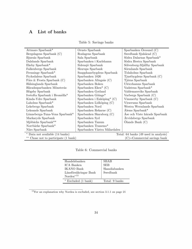
A List of banks
Table 5: Savings banks
Attmars Sparbank* Orusts Sparbank Sparbanken Oresund (C)Bergslagens Sparbank (C) Roslagens Sparbank Swedbank Sjuharad (C)Bjursas Sparbank Sala Sparbank Sodra Dalarnas Sparbank*Dalslands Sparbank Sparbanken i Karlshamn Sodra Hestra SparbankEkeby Sparbank* Sidensjo Sparbank Solvesborg-Mjallby SparbankFalkenbergs Sparbank Skurups Sparbank Sormlands SparbankFrenninge Sparbank* Snapphanebygdens Sparbank Tidaholms SparbankFryksdalens Sparbank Sparbanken 1826 Tjustbygdens Sparbank (C)Fars & Frosta Sparbank (C) Sparbanken Alingsas (C) Tjorns SparbankHalsinglands Sparbank Sparbanken Boken Ulricehamns SparbankHaradssparbanken Monsteras Sparbanken Eken* (C) Vadstena Sparbank*Hogsby Sparbank Sparbanken Gotland Valdemarsviks SparbankIvetofta Sparbank i Bromolla* Sparbanken Goinge* Varbergs Sparbank (C)Kinda-Ydre Sparbank Sparbanken i Enkoping* (C) Vimmerby Sparbank (C)Laholms Sparbank* Sparbanken Lidkoping (C) Virserums SparbankLekebergs Sparbank Sparbanken Nord Westra Wermlands SparbankLeksands Sparbank Sparbanken Rekarne (C) Alems Sparbank*Lonneberga-Tuna-Vena Sparbank* Sparbanken Skaraborg (C) Ase och Viste harads SparbankMarkaryds Sparbank Sparbanken Syd Atvidabergs Sparbank
Mjobacks Sparbank** Sparbanken Tanum Olands Bank (C)Norrbarke Sparbank* Sparbanken Tranemo*Nars Sparbank Sparbanken Vastra Malardalen∗ Data not available (14 banks) Total: 64 banks (49 used in analysis)∗∗ Chose not to participate (1 bank) (C)=Commercial savings bank
Table 6: Commercial banks
Handelsbanken SBABICA Banken SEBIKANO Bank SkandiabankenLansforsakringar Bank SwedbankNordea∗13
∗ Excluded (1 bank) Total: 9 banks
13For an explanation why Nordea is excluded, see section 3.1.1 on page 21
34
B Econometric appendix
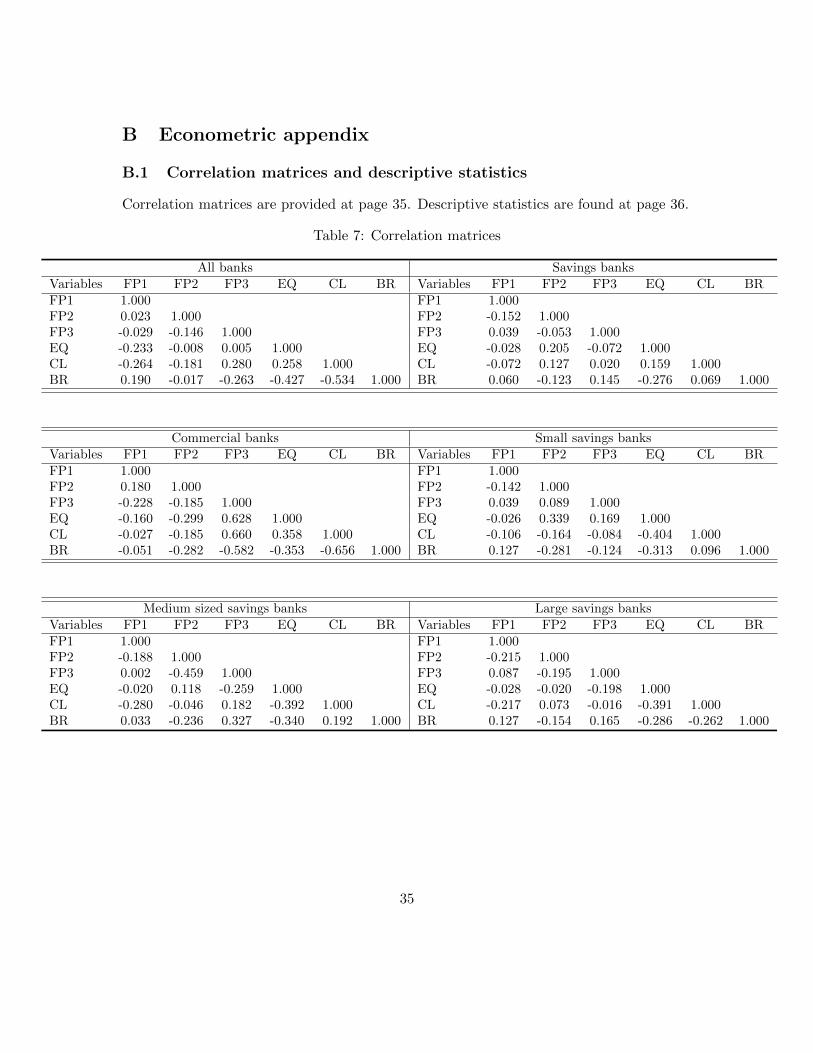
B.1 Correlation matrices and descriptive statistics
Correlation matrices are provided at page 35. Descriptive statistics are found at page 36.
Table 7: Correlation matrices
All banks Savings banksVariables FP1 FP2 FP3 EQ CL BR Variables FP1 FP2 FP3 EQ CL BRFP1 1.000 FP1 1.000FP2 0.023 1.000 FP2 -0.152 1.000FP3 -0.029 -0.146 1.000 FP3 0.039 -0.053 1.000EQ -0.233 -0.008 0.005 1.000 EQ -0.028 0.205 -0.072 1.000CL -0.264 -0.181 0.280 0.258 1.000 CL -0.072 0.127 0.020 0.159 1.000BR 0.190 -0.017 -0.263 -0.427 -0.534 1.000 BR 0.060 -0.123 0.145 -0.276 0.069 1.000
Commercial banks Small savings banksVariables FP1 FP2 FP3 EQ CL BR Variables FP1 FP2 FP3 EQ CL BRFP1 1.000 FP1 1.000FP2 0.180 1.000 FP2 -0.142 1.000FP3 -0.228 -0.185 1.000 FP3 0.039 0.089 1.000EQ -0.160 -0.299 0.628 1.000 EQ -0.026 0.339 0.169 1.000CL -0.027 -0.185 0.660 0.358 1.000 CL -0.106 -0.164 -0.084 -0.404 1.000BR -0.051 -0.282 -0.582 -0.353 -0.656 1.000 BR 0.127 -0.281 -0.124 -0.313 0.096 1.000
Medium sized savings banks Large savings banksVariables FP1 FP2 FP3 EQ CL BR Variables FP1 FP2 FP3 EQ CL BRFP1 1.000 FP1 1.000FP2 -0.188 1.000 FP2 -0.215 1.000FP3 0.002 -0.459 1.000 FP3 0.087 -0.195 1.000EQ -0.020 0.118 -0.259 1.000 EQ -0.028 -0.020 -0.198 1.000CL -0.280 -0.046 0.182 -0.392 1.000 CL -0.217 0.073 -0.016 -0.391 1.000BR 0.033 -0.236 0.327 -0.340 0.192 1.000 BR 0.127 -0.154 0.165 -0.286 -0.262 1.000
35
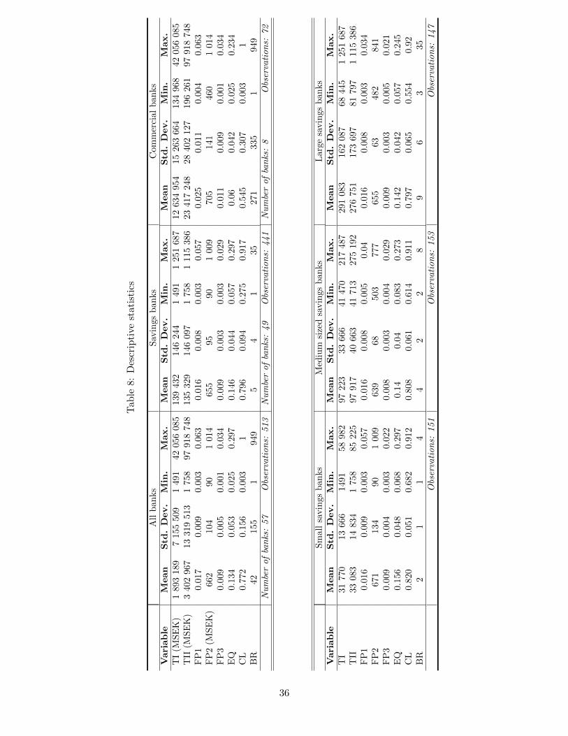
Tab
le8:
Des
crip
tive
stat
isti
cs
All
ban
ks
Sav
ings
ban
ks
Com
mer
cial
ban
ks
Vari
ab
leM
ean
Std
.D
ev.
Min
.M
ax.
Mean
Std
.D
ev.
Min
.M
ax.
Mean
Std
.D
ev.
Min
.M
ax.
TI
(MS
EK
)1
893
189
715
550
91
491
4205
608
5139
432
146
244
1491
125
1687
12
634
954
15
263
664
134
968
42
056
085
TII
(MS
EK
)3
402
967
1331
951
31
758
9791
874
8135
329
146
097
1758
111
5386
23
417
248
28
402
127
196
261
97
918
748
FP
10.
017
0.00
90.
003
0.06
30.0
16
0.0
08
0.0
03
0.057
0.0
25
0.0
11
0.0
04
0.0
63
FP
2(M
SE
K)
662
104
901
014
655
95
90
1009
705
141
460
1014
FP
30.
009
0.00
50.
001
0.03
40.0
09
0.0
03
0.0
03
0.029
0.0
11
0.0
09
0.0
01
0.0
34
EQ
0.13
40.
053
0.02
50.
297
0.1
46
0.0
44
0.0
57
0.297
0.0
60.0
42
0.0
25
0.2
34
CL
0.77
20.
156
0.00
31
0.7
96
0.0
94
0.2
75
0.917
0.5
45
0.3
07
0.0
03
1B
R42
155
194
95
41
35
271
335
1949
Nu
mbe
rof
ban
ks:
57
Obs
erva
tion
s:513
Nu
mbe
rof
ban
ks:
49
Obs
erva
tion
s:441
Nu
mbe
rof
ban
ks:
8O
bser
vati
on
s:72
Sm
all
savin
gsb
anks
Med
ium
size
dsa
vin
gs
ban
ks
Larg
esa
vin
gs
ban
ks
Vari
ab
leM
ean
Std
.D
ev.
Min
.M
ax.
Mean
Std
.D
ev.
Min
.M
ax.
Mean
Std
.D
ev.
Min
.M
ax.
TI
3177
013
666
1491
5898
297
223
33
666
41
470
217
487
291
083
162
087
68
445
1251
687
TII
3308
314
834
175
885
225
97
917
40
663
41
713
275
192
276
751
173
697
81
797
1115
386
FP
10.
016
0.00
90.
003
0.05
70.0
16
0.0
08
0.0
05
0.0
40.0
16
0.0
08
0.0
03
0.0
34
FP
267
113
490
100
9639
68
503
777
655
63
482
841
FP
30.
009
0.00
40.
003
0.02
20.0
08
0.0
03
0.0
04
0.029
0.0
09
0.0
03
0.0
05
0.0
21
EQ
0.15
60.
048
0.06
80.
297
0.1
40.0
40.0
83
0.2
73
0.1
42
0.0
42
0.0
57
0.2
45
CL
0.82
00.
051
0.68
20.
912
0.8
08
0.0
61
0.6
14
0.911
0.7
97
0.0
65
0.5
54
0.9
2B
R2
11
44
22
89
63
35
Obs
erva
tion
s:151
Obs
erva
tion
s:153
Obs
erva
tion
s:147
36
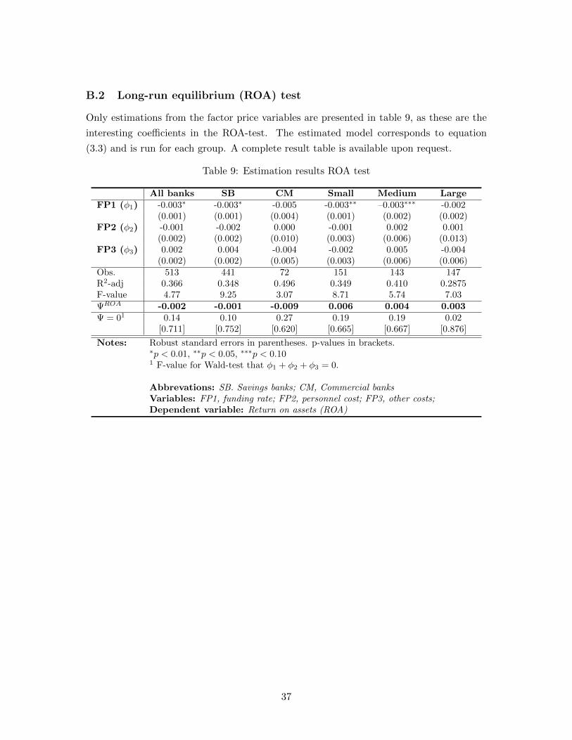
B.2 Long-run equilibrium (ROA) test
Only estimations from the factor price variables are presented in table 9, as these are the
interesting coefficients in the ROA-test. The estimated model corresponds to equation
(3.3) and is run for each group. A complete result table is available upon request.
Table 9: Estimation results ROA test
All banks SB CM Small Medium LargeFP1 (φ1) -0.003∗ -0.003∗ -0.005 -0.003∗∗ –0.003∗∗∗ -0.002
(0.001) (0.001) (0.004) (0.001) (0.002) (0.002)FP2 (φ2) -0.001 -0.002 0.000 -0.001 0.002 0.001
(0.002) (0.002) (0.010) (0.003) (0.006) (0.013)FP3 (φ3) 0.002 0.004 -0.004 -0.002 0.005 -0.004
(0.002) (0.002) (0.005) (0.003) (0.006) (0.006)Obs. 513 441 72 151 143 147R2-adj 0.366 0.348 0.496 0.349 0.410 0.2875F-value 4.77 9.25 3.07 8.71 5.74 7.03ΨROA -0.002 -0.001 -0.009 0.006 0.004 0.003Ψ = 01 0.14 0.10 0.27 0.19 0.19 0.02
[0.711] [0.752] [0.620] [0.665] [0.667] [0.876]
Notes: Robust standard errors in parentheses. p-values in brackets.∗p < 0.01, ∗∗p < 0.05, ∗∗∗p < 0.101 F-value for Wald-test that φ1 + φ2 + φ3 = 0.
Abbrevations: SB. Savings banks; CM, Commercial banksVariables: FP1, funding rate; FP2, personnel cost; FP3, other costs;Dependent variable: Return on assets (ROA)
37
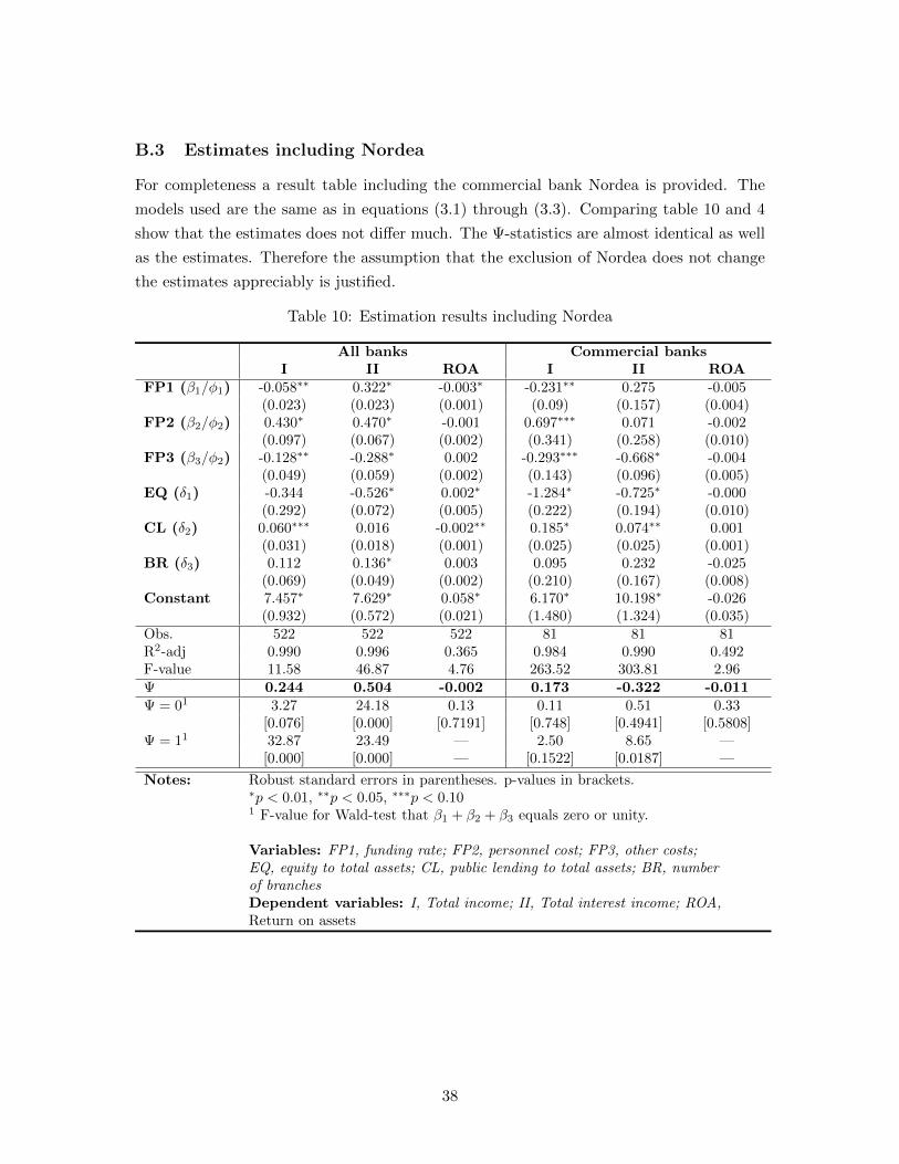
B.3 Estimates including Nordea
For completeness a result table including the commercial bank Nordea is provided. The
models used are the same as in equations (3.1) through (3.3). Comparing table 10 and 4
show that the estimates does not differ much. The Ψ-statistics are almost identical as well
as the estimates. Therefore the assumption that the exclusion of Nordea does not change
the estimates appreciably is justified.
Table 10: Estimation results including Nordea
All banks Commercial banksI II ROA I II ROA
FP1 (β1/φ1) -0.058∗∗ 0.322∗ -0.003∗ -0.231∗∗ 0.275 -0.005(0.023) (0.023) (0.001) (0.09) (0.157) (0.004)
FP2 (β2/φ2) 0.430∗ 0.470∗ -0.001 0.697∗∗∗ 0.071 -0.002(0.097) (0.067) (0.002) (0.341) (0.258) (0.010)
FP3 (β3/φ2) -0.128∗∗ -0.288∗ 0.002 -0.293∗∗∗ -0.668∗ -0.004(0.049) (0.059) (0.002) (0.143) (0.096) (0.005)
EQ (δ1) -0.344 -0.526∗ 0.002∗ -1.284∗ -0.725∗ -0.000(0.292) (0.072) (0.005) (0.222) (0.194) (0.010)
CL (δ2) 0.060∗∗∗ 0.016 -0.002∗∗ 0.185∗ 0.074∗∗ 0.001(0.031) (0.018) (0.001) (0.025) (0.025) (0.001)
BR (δ3) 0.112 0.136∗ 0.003 0.095 0.232 -0.025(0.069) (0.049) (0.002) (0.210) (0.167) (0.008)
Constant 7.457∗ 7.629∗ 0.058∗ 6.170∗ 10.198∗ -0.026(0.932) (0.572) (0.021) (1.480) (1.324) (0.035)
Obs. 522 522 522 81 81 81R2-adj 0.990 0.996 0.365 0.984 0.990 0.492F-value 11.58 46.87 4.76 263.52 303.81 2.96Ψ 0.244 0.504 -0.002 0.173 -0.322 -0.011Ψ = 01 3.27 24.18 0.13 0.11 0.51 0.33
[0.076] [0.000] [0.7191] [0.748] [0.4941] [0.5808]Ψ = 11 32.87 23.49 — 2.50 8.65 —
[0.000] [0.000] — [0.1522] [0.0187] —
Notes: Robust standard errors in parentheses. p-values in brackets.∗p < 0.01, ∗∗p < 0.05, ∗∗∗p < 0.101 F-value for Wald-test that β1 + β2 + β3 equals zero or unity.
Variables: FP1, funding rate; FP2, personnel cost; FP3, other costs;EQ, equity to total assets; CL, public lending to total assets; BR, numberof branchesDependent variables: I, Total income; II, Total interest income; ROA,Return on assets
38
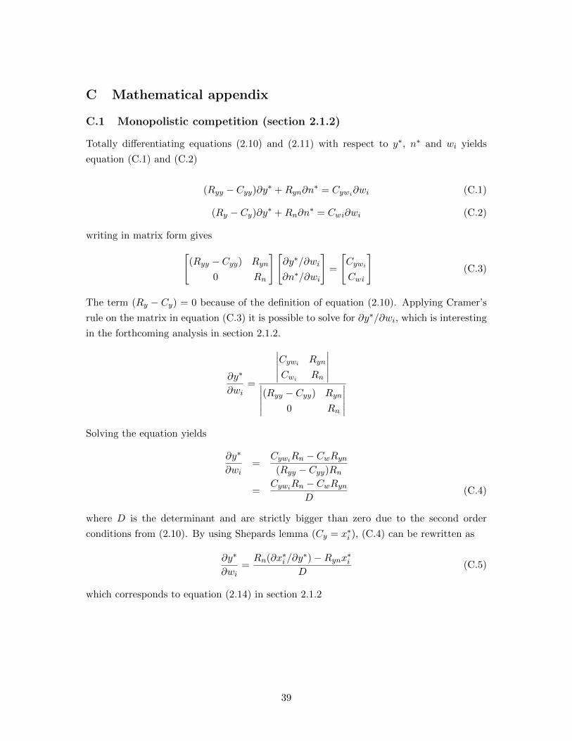
C Mathematical appendix
C.1 Monopolistic competition (section 2.1.2)
Totally differentiating equations (2.10) and (2.11) with respect to y∗, n∗ and wi yields
equation (C.1) and (C.2)
(Ryy − Cyy)∂y∗ +Ryn∂n∗ = Cywi∂wi (C.1)
(Ry − Cy)∂y∗ +Rn∂n∗ = Cwi∂wi (C.2)
writing in matrix form gives[(Ryy − Cyy) Ryn
0 Rn
][∂y∗/∂wi
∂n∗/∂wi
]=
[Cywi
Cwi
](C.3)
The term (Ry − Cy) = 0 because of the definition of equation (2.10). Applying Cramer’s
rule on the matrix in equation (C.3) it is possible to solve for ∂y∗/∂wi, which is interesting
in the forthcoming analysis in section 2.1.2.
∂y∗
∂wi=
∣∣∣∣∣Cywi Ryn
Cwi Rn
∣∣∣∣∣∣∣∣∣∣(Ryy − Cyy) Ryn
0 Rn
∣∣∣∣∣Solving the equation yields
∂y∗
∂wi=
CywiRn − CwRyn
(Ryy − Cyy)Rn
=CywiRn − CwRyn
D(C.4)
where D is the determinant and are strictly bigger than zero due to the second order
conditions from (2.10). By using Shepards lemma (Cy = x∗i ), (C.4) can be rewritten as
∂y∗
∂wi=Rn(∂x∗i /∂y
∗)−Rynx∗i
D(C.5)
which corresponds to equation (2.14) in section 2.1.2
39
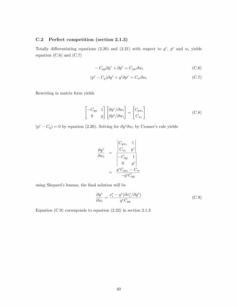
C.2 Perfect competition (section 2.1.3)
Totally differentiating equations (2.20) and (2.21) with respect to yc, pc and wi yields
equation (C.6) and (C.7)
− Cyy∂yc + ∂pc = Cyw∂wi (C.6)
(pc − Cy)∂yc + yc∂pc = Cw∂wi (C.7)
Rewriting in matrix form yields
[−Cyy 1
0 y
][∂yc/∂wi
∂pc/∂wi
]=
[Cywi
Cwi
](C.8)
(pc − Cy) = 0 by equation (2.20). Solving for ∂yc∂wi by Cramer’s rule yields
∂yc
∂wi=
∣∣∣∣∣Cywi 1
Cwi yc
∣∣∣∣∣∣∣∣∣∣−Cyy 1
0 yc
∣∣∣∣∣=
ycCywi − Cw
−ycCyy
using Shepard’s lemma, the final solution will be
∂yc
∂wi=x∗i − yc(∂x∗i /∂yc)
ycCyy(C.9)
Equation (C.9) corresponds to equation (2.22) in section 2.1.3
40