Scaling up population dynamics: integrating theory and …€¦Melbourne BA, Chesson P (in press). Scaling up population dynamics: integrating theory and data. Oecologia. 2 Abstract

Scaling up population dynamics: integrating theory and data Brett A. Melbourne and Peter Chesson Mailing Address:

Brett A. Melbourne Center for Population Biology Storer Hall University of California, Davis, CA 95616

Phone (530) 752-6837; Fax (530) 752-3350; [email protected] Affiliations: Brett A. Melbourne Center for Population Biology, University of California, Davis [email protected] Peter Chesson Section of Evolution and Ecology, University of California, Davis [email protected] Running head: Scaling up population dynamics Revised accepted: 7 September 2004 Invited contribution to special issue of Oecologia on scaling up population dynamics. Citation: Melbourne BA, Chesson P (in press). Scaling up population dynamics: integrating theory and data. Oecologia.

Melbourne BA, Chesson P (in press). Scaling up population dynamics: integrating theory and data. Oecologia.

2

Abstract How to scale up from local scale interactions to regional scale dynamics is a critical issue in field ecology. We show how to implement a systematic approach to the problem of scaling up, using scale transition theory. Scale transition theory shows that dynamics on larger spatial scales differ from predictions based on local dynamics alone because of an interaction between local scale nonlinear dynamics and spatial variation in density or the environment. Based on this theory, a systematic approach to scaling up has four steps: 1) derive a model to translate the effects of local dynamics to the regional scale, and to identify key interactions between nonlinearity and spatial variation, 2) measure local-scale model parameters to determine nonlinearities at local scales, 3) measure spatial variation, 4) combine nonlinearity and variation measures to obtain the scale transition. We illustrate the approach with an example from benthic stream ecology of caddisflies living in riffles. By sampling from a simulated system, we show how collecting the appropriate data at local (riffle) scales to measure nonlinearities, combined with measures of spatial variation, leads to the correct inference for dynamics at the larger scale of the stream. The approach provides a way to investigate the mechanisms and consequences of changes in population dynamics with spatial scale using a relatively small amount of field data. Keywords: heterogeneity, nonlinear dynamics, scale, spatial ecology.

Introduction A vexing problem in ecology is how to make predictions for population dynamics at large spatial scales based on information gained at small spatial scales, because small scale trends in population dynamics are often contradicted by large scale outcomes (e.g. Chesson 1996; Englund and Cooper 2003). At the most fundamental level, scale transition theory shows that the majority of the important changes in population dynamics that arise with such changes in scale can be attributed to an interaction between local-scale nonlinear population dynamics and spatial variation in either population density or the physical environment (Chesson 1978; 1996; 1998a; 1998b; 2001; Chesson et al. in press). This interaction has been shown in theoretical models to promote stability, persistence, and coexistence on larger spatial scales, contrary to predictions of small scale dynamics alone (Chesson 2000; De Jong 1979; Hassell et al. 1991; Ives 1988; Pacala and Levin 1997). This interaction means also that quantitative features, such as the large-scale carrying capacity, are different from the small scale predictions (e.g. Bolker and Pacala 1997; Chesson 1998b; De Jong 1979). Measuring the theoretically predicted interaction between nonlinearity and variation provides a way to understand linkages between scales and to scale up population dynamics from local to regional scales. Furthermore, measuring this interaction provides a general test of spatial mechanisms in population dynamics. As it is relatively straight forward to quantify local nonlinearities and spatial variation, it is possible to measure their interaction in field studies. The fundamentals of scale transition theory are described in Chesson (1978; 1996; 1998a; 1998b) and Chesson et al. (in press). Here we emphasize how scale transition theory is used with data. Special cases of the general scale transition methods presented here have been discovered from time to time by others beginning with Lloyd and White (1980) and more recently exemplified by


3

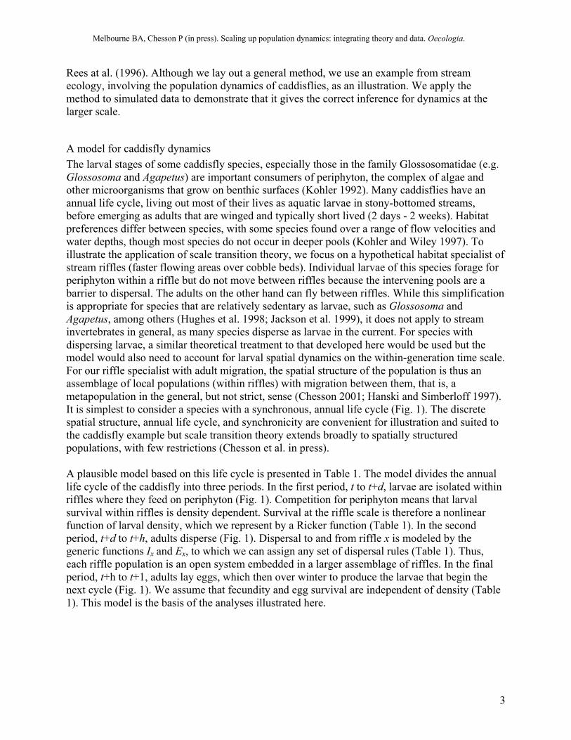
Rees at al. (1996). Although we lay out a general method, we use an example from stream ecology, involving the population dynamics of caddisflies, as an illustration. We apply the method to simulated data to demonstrate that it gives the correct inference for dynamics at the larger scale.

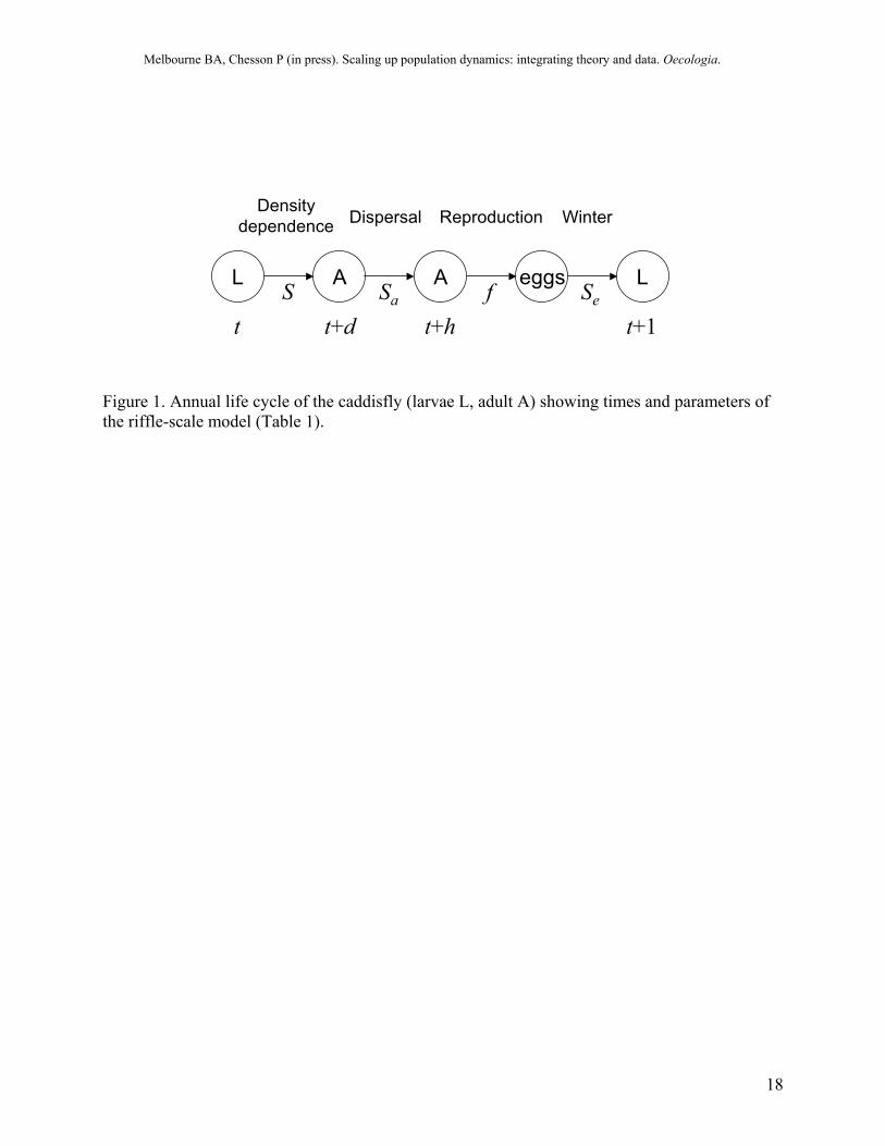
A model for caddisfly dynamics The larval stages of some caddisfly species, especially those in the family Glossosomatidae (e.g. Glossosoma and Agapetus) are important consumers of periphyton, the complex of algae and other microorganisms that grow on benthic surfaces (Kohler 1992). Many caddisflies have an annual life cycle, living out most of their lives as aquatic larvae in stony-bottomed streams, before emerging as adults that are winged and typically short lived (2 days - 2 weeks). Habitat preferences differ between species, with some species found over a range of flow velocities and water depths, though most species do not occur in deeper pools (Kohler and Wiley 1997). To illustrate the application of scale transition theory, we focus on a hypothetical habitat specialist of stream riffles (faster flowing areas over cobble beds). Individual larvae of this species forage for periphyton within a riffle but do not move between riffles because the intervening pools are a barrier to dispersal. The adults on the other hand can fly between riffles. While this simplification is appropriate for species that are relatively sedentary as larvae, such as Glossosoma and Agapetus, among others (Hughes et al. 1998; Jackson et al. 1999), it does not apply to stream invertebrates in general, as many species disperse as larvae in the current. For species with dispersing larvae, a similar theoretical treatment to that developed here would be used but the model would also need to account for larval spatial dynamics on the within-generation time scale. For our riffle specialist with adult migration, the spatial structure of the population is thus an assemblage of local populations (within riffles) with migration between them, that is, a metapopulation in the general, but not strict, sense (Chesson 2001; Hanski and Simberloff 1997). It is simplest to consider a species with a synchronous, annual life cycle (Fig. 1). The discrete spatial structure, annual life cycle, and synchronicity are convenient for illustration and suited to the caddisfly example but scale transition theory extends broadly to spatially structured populations, with few restrictions (Chesson et al. in press). A plausible model based on this life cycle is presented in Table 1. The model divides the annual life cycle of the caddisfly into three periods. In the first period, t to t+d, larvae are isolated within riffles where they feed on periphyton (Fig. 1). Competition for periphyton means that larval survival within riffles is density dependent. Survival at the riffle scale is therefore a nonlinear function of larval density, which we represent by a Ricker function (Table 1). In the second period, t+d to t+h, adults disperse (Fig. 1). Dispersal to and from riffle x is modeled by the generic functions Ix and Ex, to which we can assign any set of dispersal rules (Table 1). Thus, each riffle population is an open system embedded in a larger assemblage of riffles. In the final period, t+h to t+1, adults lay eggs, which then over winter to produce the larvae that begin the next cycle (Fig. 1). We assume that fecundity and egg survival are independent of density (Table 1). This model is the basis of the analyses illustrated here.


4

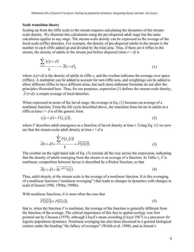
Scale transition theory Scaling up from the riffle scale to the stream requires calculating the dynamics of the stream-scale density. We illustrate this calculation using the pre-dispersal adult stage but the same calculation applies to any stage. The stream-scale density can be expressed as the average of the local-scale (riffle) densities. For example, the density of pre-dispersal adults in the stream is the number in each riffle added up and divided by the total area. Thus, if there are k riffles in the stream, the density of adults in the stream just before dispersal (time t + d) is

( )

( )dtAk

dtAk

xx

+=+∑

=1 , (1)

where Ax(t+d) is the density of adults in riffle x, and the overbar indicates the average over space (riffles). A multiplier can be added to account for non-riffle area, and weightings can be added to allow different riffles to have different areas, but such more elaborate formulae do not alter the principles illustrated here. Thus, for our purposes, expression (1) defines the stream-scale density, A (t+d): a simple average of local densities. When expressed in terms of the larval stage, the average in Eq. (1) becomes an average of a nonlinear function. From the life cycle described above, the transition from larvae to adults in a riffle at time t + d is of the generic form

( ) ( )( )tLFdtA xx =+ , (2)

where F describes adult emergence as a function of larval density at time t. Using Eq. (1) we now see that the stream-scale adult density at time t + d is

( )( )( )

( )( )tLFk

tLFdtA

k

xx

==+∑=1 . (3)

The overbar on the right hand side of Eq. (3) extends all the way across the expression, indicating that the density of adults emerging from the stream is an average of a function. In Table 1, F is nonlinear; competition between larvae is described by a Ricker function, so that

( ) ( ) ( )tLSedtA tLα−=+ . (4)

Thus, adult density at the stream scale is the average of a nonlinear function. It is this averaging of a nonlinear function (“nonlinear averaging”) that leads to changes in dynamics with changes in scale (Chesson 1996; 1998a; 1998b). With nonlinear functions, it is most often the case that

( )( ) ( )( )tLFtLF ≠ , (5)

that is, when the function F is nonlinear, the average of the function is generally different from the function of the average. The critical importance of this fact to spatial ecology was first pointed out by Chesson (1978), although Lloyd’s mean crowding (Lloyd 1967) is a precursor for logistic population dynamics. Nonlinear averaging has also been discussed in a general biological context under the heading “the fallacy of averages” (Welsh et al. 1988), and as Jensen’s


5

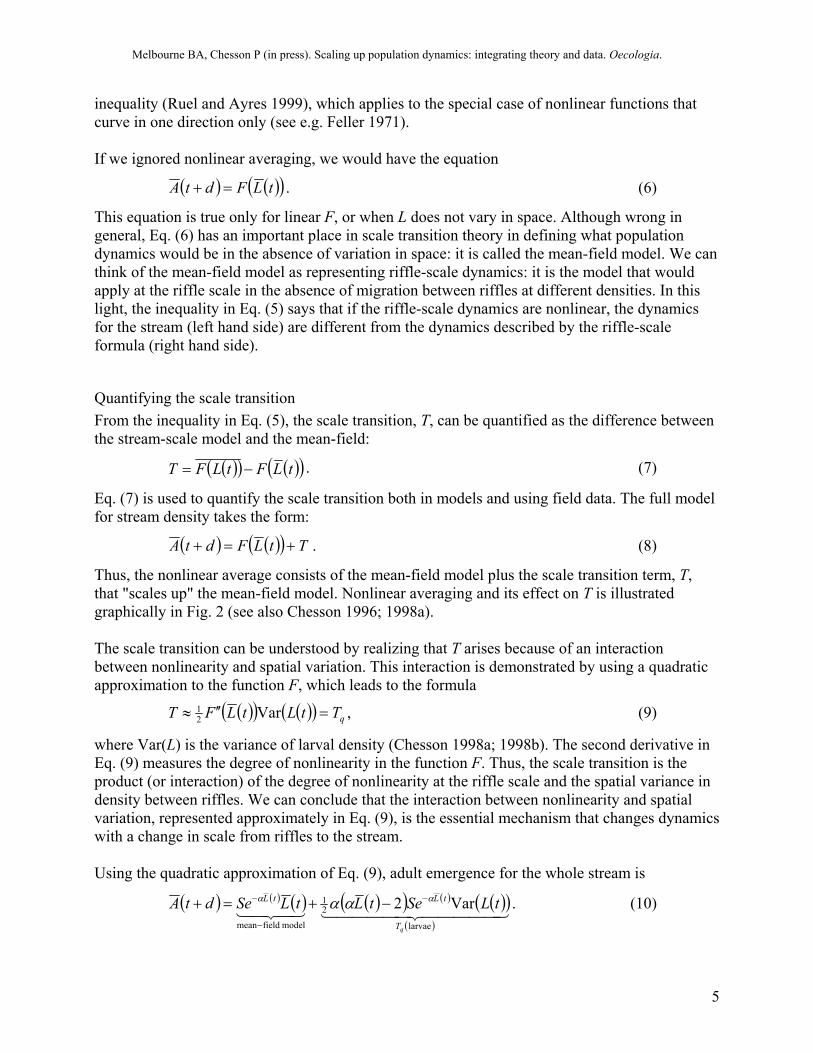
inequality (Ruel and Ayres 1999), which applies to the special case of nonlinear functions that curve in one direction only (see e.g. Feller 1971). If we ignored nonlinear averaging, we would have the equation

( ) ( )( )tLFdtA =+ . (6)

This equation is true only for linear F, or when L does not vary in space. Although wrong in general, Eq. (6) has an important place in scale transition theory in defining what population dynamics would be in the absence of variation in space: it is called the mean-field model. We can think of the mean-field model as representing riffle-scale dynamics: it is the model that would apply at the riffle scale in the absence of migration between riffles at different densities. In this light, the inequality in Eq. (5) says that if the riffle-scale dynamics are nonlinear, the dynamics for the stream (left hand side) are different from the dynamics described by the riffle-scale formula (right hand side).

Quantifying the scale transition From the inequality in Eq. (5), the scale transition, T, can be quantified as the difference between the stream-scale model and the mean-field:

( )( ) ( )( )tLFtLFT −= . (7)

Eq. (7) is used to quantify the scale transition both in models and using field data. The full model for stream density takes the form:

( ) ( )( ) TtLFdtA +=+ . (8)

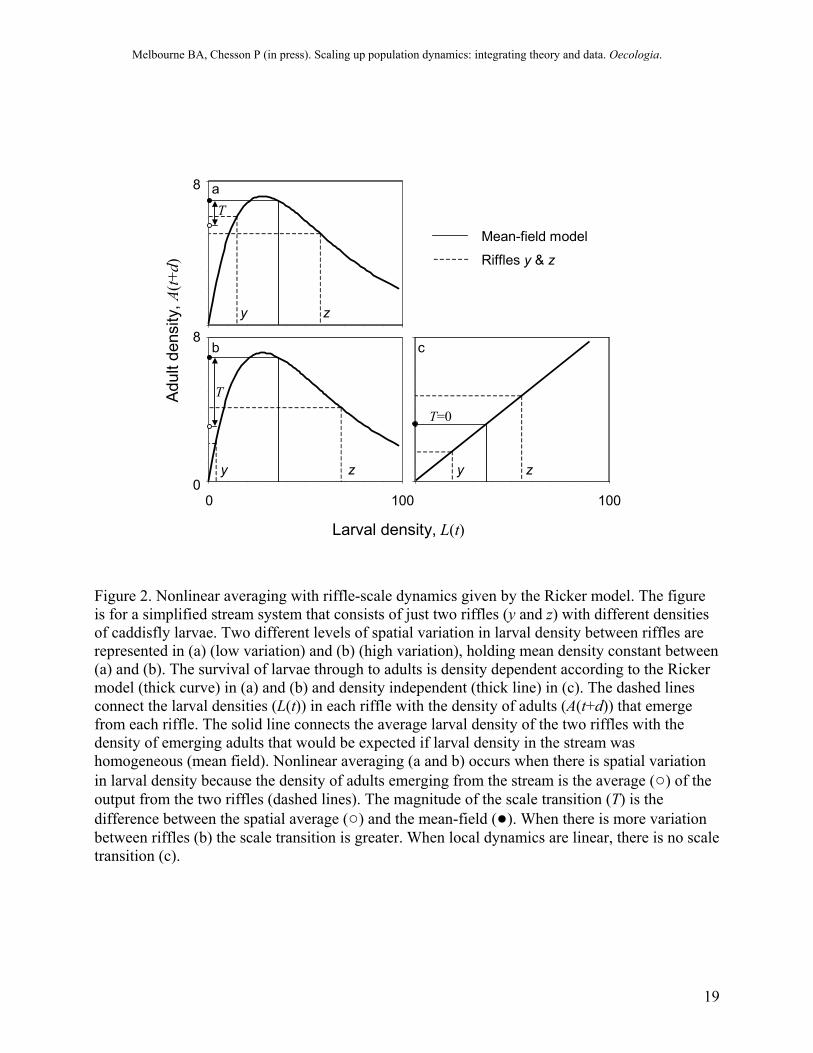
Thus, the nonlinear average consists of the mean-field model plus the scale transition term, T, that "scales up" the mean-field model. Nonlinear averaging and its effect on T is illustrated graphically in Fig. 2 (see also Chesson 1996; 1998a). The scale transition can be understood by realizing that T arises because of an interaction between nonlinearity and spatial variation. This interaction is demonstrated by using a quadratic approximation to the function F, which leads to the formula

( )( ) ( )( ) qTtLtLFT =′′≈ Var21 , (9)

where Var(L) is the variance of larval density (Chesson 1998a; 1998b). The second derivative in Eq. (9) measures the degree of nonlinearity in the function F. Thus, the scale transition is the product (or interaction) of the degree of nonlinearity at the riffle scale and the spatial variance in density between riffles. We can conclude that the interaction between nonlinearity and spatial variation, represented approximately in Eq. (9), is the essential mechanism that changes dynamics with a change in scale from riffles to the stream. Using the quadratic approximation of Eq. (9), adult emergence for the whole stream is

( ) ( ) ( ) ( )( ) ( ) ( )( )( )

44444 344444 2143421larvae

21

model fieldmean

Var2qT

tLtL tLSetLtLSedtA αα αα −

−

− −+=+ . (10)


6

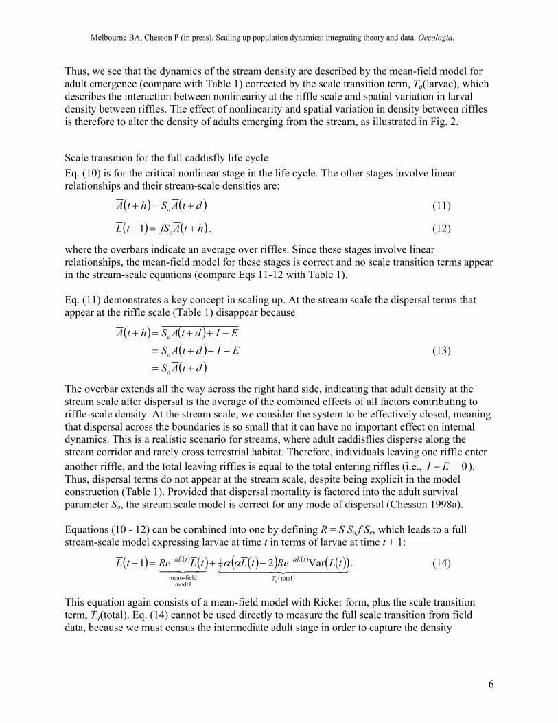
Thus, we see that the dynamics of the stream density are described by the mean-field model for adult emergence (compare with Table 1) corrected by the scale transition term, Tq(larvae), which describes the interaction between nonlinearity at the riffle scale and spatial variation in larval density between riffles. The effect of nonlinearity and spatial variation in density between riffles is therefore to alter the density of adults emerging from the stream, as illustrated in Fig. 2.

Scale transition for the full caddisfly life cycle Eq. (10) is for the critical nonlinear stage in the life cycle. The other stages involve linear relationships and their stream-scale densities are:

( ) ( )dtAShtA a +=+ (11)

( ) ( )htAfStL e +=+1 , (12)

where the overbars indicate an average over riffles. Since these stages involve linear relationships, the mean-field model for these stages is correct and no scale transition terms appear in the stream-scale equations (compare Eqs 11-12 with Table 1). Eq. (11) demonstrates a key concept in scaling up. At the stream scale the dispersal terms that appear at the riffle scale (Table 1) disappear because

( ) ( )

( )( ).dtAS

EIdtASEIdtAShtA

a

a

a

+=

−++=

−++=+

(13)

The overbar extends all the way across the right hand side, indicating that adult density at the stream scale after dispersal is the average of the combined effects of all factors contributing to riffle-scale density. At the stream scale, we consider the system to be effectively closed, meaning that dispersal across the boundaries is so small that it can have no important effect on internal dynamics. This is a realistic scenario for streams, where adult caddisflies disperse along the stream corridor and rarely cross terrestrial habitat. Therefore, individuals leaving one riffle enter another riffle, and the total leaving riffles is equal to the total entering riffles (i.e., 0=− EI ). Thus, dispersal terms do not appear at the stream scale, despite being explicit in the model construction (Table 1). Provided that dispersal mortality is factored into the adult survival parameter Sa, the stream scale model is correct for any mode of dispersal (Chesson 1998a). Equations (10 - 12) can be combined into one by defining R = S Sa f Se, which leads to a full stream-scale model expressing larvae at time t in terms of larvae at time t + 1:

( ) ( ) ( ) ( )( ) ( ) ( )( )( )

44444 344444 2143421total

21

modelfield-mean

Var21qT

tLtL tLRetLtLRetL αα αα −− −+=+ . (14)

This equation again consists of a mean-field model with Ricker form, plus the scale transition term, Tq(total). Eq. (14) cannot be used directly to measure the full scale transition from field data, because we must census the intermediate adult stage in order to capture the density


7

dependent process. Thus, to measure the scale transition from field data, we first need to use Eq. (10) to calculate the scale transition for the larval stage.

Spatial simulation of the stream metapopulation To demonstrate the application of scale transition theory, we simulate the caddisfly system using the model in Table 1. The form of migration between riffles is not specified there. To specify migration we imagine that all adults disperse, and immigration into a riffle is determined by the environmental attractiveness of the riffle to an adult. For example, attractiveness might involve the suitability of surrounding vegetation. To simulate this, we assign each riffle an attractiveness value by drawing a random number from a standard gamma distribution. Then, individuals from the global pool immigrate to riffles according to a Poisson process with rate parameter equal to the attractiveness value, until all individuals from the global pool have dispersed back to a riffle. For a large number of riffles (we use 1000), this mode of dispersal results in a negative binomial distribution for the adults after dispersal, where the aggregation parameter, k, of the negative binomial is the shape parameter of the gamma distribution (Chesson 1998a). We use realistic values for the parameters in Table 1 from data in Marchant (1999) for the caddisfly Agapetus monticolus (α = 0.036, S = 0.7, f = 25, SaSe = 0.15 - 0.5).

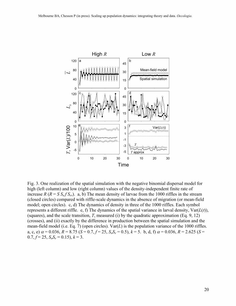
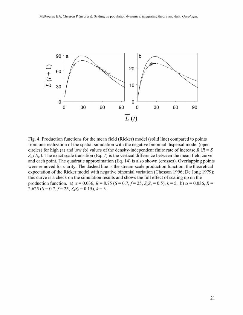
Quantifying the scale transition in the model simulation Before we discuss field data, we will examine the scale transition for the model simulation and use the scale transition model of Eq. (12) to understand the simulation results. Scaling up from riffles to the stream changes dynamics both qualitatively and quantitatively (Fig. 3). The mean-field model, which represents the riffle-scale model, has a stable limit cycle when R is moderately high (Fig. 3a). In contrast, when riffles are connected by adult migration, the stream-scale dynamics are stable with rapid convergence on an equilibrium (Fig. 3a). For a lower value of R, the qualitative nature of the dynamics is preserved in scaling up but there is a quantitative difference: the equilibrium biomass is reduced by about 15% (Fig. 3b). These changes can be traced to the interaction between nonlinearity in larval survival and spatial variation in larval density. The scale transition, T, arising from this interaction is represented by the approximate correction term, Tq(total), in Eq. (12). By simulation, T can also be measured exactly as the difference in production for the spatial simulation and the mean-field model (Eq. 7). The dynamics of T follow that of the variance (Fig 3f). For the fluctuating population with high R, T boosts production when density is high (production low) and depresses production when density is low (production high), evening out production over the range of stream scale densities and dampening the fluctuations (Fig. 3a & 4a). For the stable population with low R, T depresses production, reducing the equilibrium density (Fig. 3b & 4b). Thus, the interaction between nonlinearity and spatial variation changes the shape of the production function at the stream scale compared to the production function at the riffle scale (Fig. 4).

Quantifying the scale transition in the field Scale transition theory suggests a systematic approach to scaling up with field data that has four steps, which we illustrate with simulated data. First, derive a scale transition model to translate the effects of local dynamics to the regional scale, and to identify key interactions between


8

nonlinearity and spatial variation. Second, measure local-scale model parameters to determine nonlinearities at local scales. Third, measure spatial variances and covariances. Fourth, combine nonlinearity and variation measures to obtain the scale transition. We already have the scale transition model (Eqs 10 - 12), so we proceed to the other steps. There are two main issues in measuring nonlinearities and spatial variation in the field. First, we will not know a priori the form of nonlinearity. Second, field densities will be measured with error. There are two possible approaches to measuring nonlinearities in the field. The first approach is to perform a density manipulation experiment to control density at time t and measure the resulting density at t + d. For example, we might set up caged arenas in the stream, stocked with different densities of larvae. However, experimental control of density is not always possible and care is needed to avoid cage effects and other scaling artifacts (Englund and Cooper 2003). An alternative to experimental manipulation is to monitor riffles that encompass a range of initial larval densities and count adults as they emerge and before they disperse. For example, in the field, larval density at time t would be measured in quadrats using a standard benthic sample net, and the density of adults emerging at time t + d would be measured using standard emergence traps. We demonstrate the monitoring approach here.

Field sampling The sample design requires sufficient local populations (riffles) to encompass a range of initial densities, and replicate samples within a riffle to estimate measurement error. We need to account for measurement error because it affects the estimation of both nonlinearities and spatial variance in density. A range of sample designs are possible. A simple and efficient design is to select n riffles at random with m random samples per riffle to give a total of n x m samples. This design allows estimation of both nonlinearities and spatial variance in density using the same data. We demonstrate measuring the scale transition for one annual cycle. To simulate field sampling we generated artificial data, corresponding to the spatial simulation in Fig. 3b. From the 1000 riffles in the spatial simulation, we selected 40 riffles at random (i.e. the sample was 4% of riffles). For each of the 40 riffles, at time t = 15 we measured larval density in 2 replicate samples, and at time t+d we measured the density of adults emerging in 2 replicate samples. To simulate samples measured with error, we introduced multiplicative error to the true densities in the simulation, so that the observed larval density L(obs) and observed adult density A(obs) were given by L(obs) = Lεl, and A(obs) = Aεa, where εl and εa are larval and adult observation error respectively, and ln(ε) is a normal random variable with variance 0.02, corresponding to measurement error of about 14%.

Estimating riffle-scale model parameters As we don’t know the nature of the nonlinearity in larval survival, a good strategy is to propose several functional forms and determine which accords best with the data (Hilborn and Mangel 1997). Including a linear model among these models serves as an alternative to the hypothesis that dynamics are nonlinear. Here, as examples, as well as the Ricker model (Table 1), we fitted the Beverton-Holt model


9

( ) ( ) ( )tLtcL

SdtA xx

x +=+

1, (15)

and the linear model (i.e. density independent survival)

( ) ( )tLSdtA xx =+ . (16)

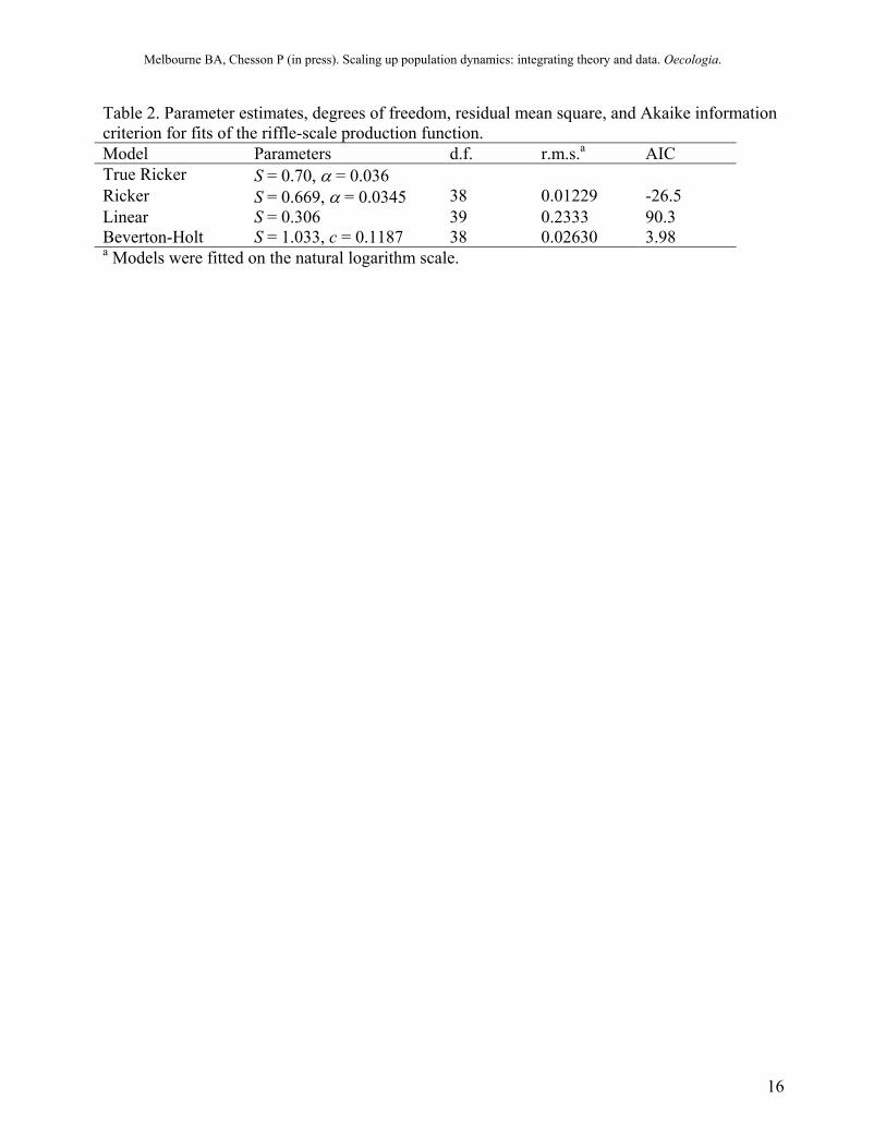
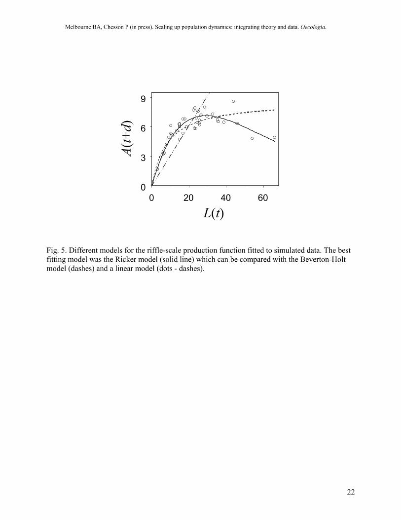
The models were fitted to the data using standard maximum likelihood methods. The best-fitting model was determined using the Akaike information criterion (AIC). For the artificially generated dataset, the best-fitting model for the local production function was clearly the Ricker model (Fig. 5), which had the lowest AIC (Table 2). The linear model was a poor fit to the data (Fig. 5, Table 2). The estimated parameter values for the Ricker model were close to the known parameter values in the simulation (Table 2). These parameter estimates are known to be biased due to measurement error in the independent variable (larval density). For these data, the bias is negligible because the variance of the measurement error is small (~1%) compared to the variance in larval density. When the measurement error is large, a procedure such as simulation-extrapolation is needed to reduce the bias (Carroll et al. 1995).

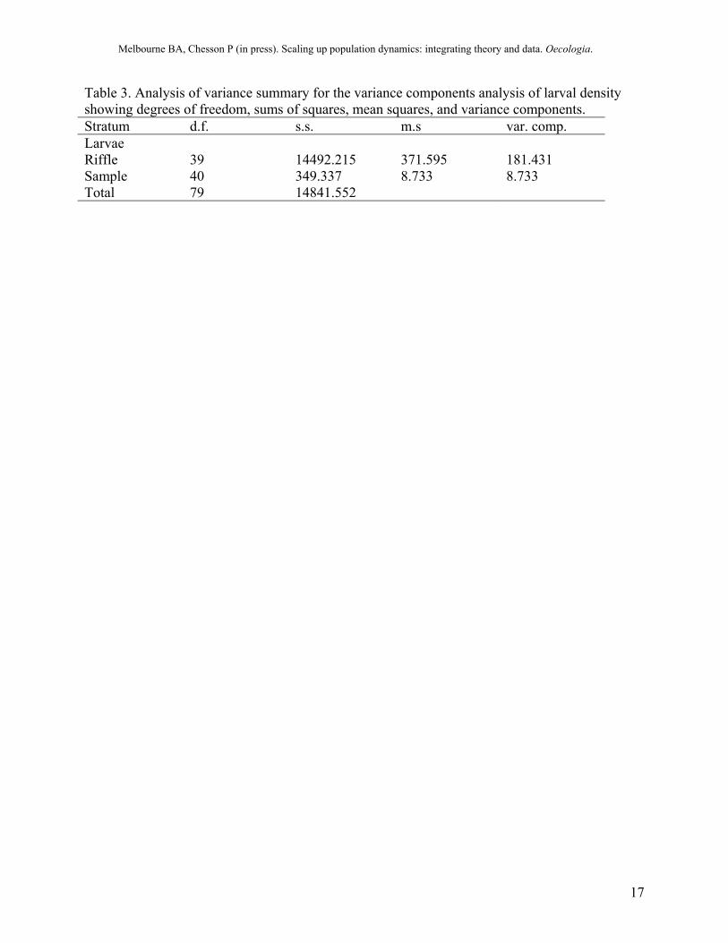
Estimating spatial variance To determine the spatial variance in density, we used hierarchical analysis of variance to decompose the variance into two variance components: the spatial variance between riffles and the variance due to measurement (sampling) error (Searle et al. 1992). The between-riffle variance was estimated to be 181.4 (Table 3), close to the true variance of all 1000 riffles measured without error in the spatial simulation of 170.4. The stream-scale larval density, estimated by the sample mean of the larval density, was 22.66, close to the true value of 22.53 measured without error in the simulation.

Combining nonlinearity and variation measures We have now sufficient information to find the quadratic approximation for the scale transition of the larval stage (Eq. 10), for this one point in time (t = 15). Substituting the parameter estimates for nonlinear survival, estimated mean larval density, and estimated variance into Eq. (10), we find that the density of adults emerging at the stream scale is 5.770. This compares to 6.937 in the mean-field model, which is estimated by substituting the parameter estimates and estimated mean larval density into the riffle-scale equation for the larval stage (Eq. 6). Thus, the estimated scale transition by the quadratic approximation, Tq(larvae), is -1.167, or -16.8%. As the remaining life history parameters in Eqs (11-12) simply apply a constant multiplier to T, this is also the proportional reduction in L (t+1) for the full life cycle in Eq. (14). An alternative to using the quadratic approximation for estimating the scale transition, is to first estimate A (t+d) using

( ) ( ) ( )∑==+n

iiLF

nLFdtA 1 , (17)


10

where F(L) is the Ricker model with the estimated parameter values, and Li is the larval density in the ith riffle of the n sampled riffles. In this approach, the data are used as an empirical surrogate for the probability distribution function of the larval densities. Equation (17) is robust to departures from quadratic nonlinearity and handles spatial heterogeneity that is not adequately summarized by the variance. The scale transition, T, is then calculated in the usual way (Eq. 7) as

( ) ( ) ( )

−=−= ∑∑n

ii

n

ii L

nFLF

nLFLFT 11 , (18)

where the second term on the right hand side is the estimated mean-field model. For these data, Eq. (18) gives T = -0.989, or -14.3%. For both the quadratic approximation and Eq. (18), the estimates for T are close to the true scale transition measured without error in the spatial simulation of -13.7%, with Eq. (18) giving the more accurate estimate.

Averaging over multiple nonlinearities Above, we have considered the case with nonlinearity from density-dependent survival and spatial variation only in population density. Scale transition theory extends to multiple nonlinearities and variation in the environment (Chesson 2000; Chesson et al. in press). Then, scale transition equations involve multiple scale transition terms. For example, differences between riffles in resource productivity (e.g. from shading) could lead to variation between riffles in the per capita competitive effects of larvae (i.e. variation in α); or variation between riffles in disturbance intensity (Downes et al. 1998) could affect larval survival, independently of larval density and competition. For the case of variation in survival, pre-dispersal adult density for a riffle is then

( ) ( ) ( )tLxxx

xetLSdtA α−=+ , (19)

where Sx represents the riffle specific effect of disturbance intensity on larval survival. The scale transition equation for Eq. (19) is

( ) ( ) ( ) ( )( ) ( ) ( )( )

( )( ) ( )( )444 3444 21

44444 344444 2143421

b

a

T

T

tLtL

tLStLg

tLeStLetLSdtA

,Cov

Var221

modelfield-mean

′+

−+=+ −− αα αα

, (20)

where g(Lx(t)) = Lx(t)exp(-αLx(t)). Thus, as before, the stream-scale model is the mean-field model plus scale transition terms. The first scale transition term, Ta, is due to the interaction of density dependence and variation in density, as before (Eq. 10), while Tb is due to the joint variation of disturbance and density dependence. The second term shows that scaling up from riffles to the stream depends on the spatial covariance between disturbance regime and larval density. As either scale transition term could be positive or negative, the two terms could have either conflicting or reinforcing effects on stream dynamics. Spatial variation in the competition parameter, α, similarly gives rise to extra scale transition terms.

These scale transition terms can be thought of as representing different spatial mechanisms. With multiple mechanisms, an analysis of the scale transition involves not only determining the total


11

effect of spatial dynamics but the relative contribution of the different mechanisms. To measure the scale transition terms using field data, the approach is not very different from before except that now we need to allow for S or α to vary between riffles. Melbourne et al. (in press) present examples of estimating multiple scale transition terms in the field.

Discussion In the examples above, we have demonstrated the concepts and properties of the scale transition in translating the effects of local scale processes to the larger scale where local populations are linked by dispersal. We outlined a four step approach to scaling up based on scale transition theory: derive a model to scale up, measure nonlinearities, measure spatial variances and covariances, and combine nonlinearity and variation measures to obtain the scale transition. In the caddisfly examples, the model at the larger scale of the stream always consisted of a mean-field model, representing riffle-scale dynamics, modified by new terms to account for spatial variation and nonlinearity in scaling up to the stream. These scale transition terms are interactions between nonlinearities and spatial variation and represent the spatial mechanisms responsible for changing dynamics at the larger scale of the stream. The scale transition terms thus point to key quantities that can be measured in the field. In the caddisfly example, we demonstrated that these quantities are measured correctly in the field by fitting models to describe nonlinearities at the riffle scale, and using appropriate sampling and estimation methods to measure spatial variation. An important feature of scale transition theory is that, while migration within the system is not measured explicitly, migration results in the generation of spatial pattern, measured by spatial variances and covariances. The importance of spatial processes is thus measured by evaluating the magnitude of the scale transition terms in which they appear. For most systems, multiple scale transition terms will appear in equations for dynamics at the larger scale. Focusing on these fundamental scale transition terms allows the relative importance of different mechanisms to be assessed quantitatively, and facilitates comparison between different systems and different models. An advantage of the approach is that spatial mechanisms can be examined with relatively little data, and much can be gained by measurements for just one time step. In the example that simulated field sampling, the sampling interval was one time step, targeting the density dependent process in the caddisfly's life history. This snapshot was sufficient to demonstrate that a significant interaction between nonlinearity and spatial variation was present. Sampling in multiple years would provide further insight. If sampling were continued for say, the following two years, we would find that the scale transition, T, remained close to 15%, causing the stream-scale carrying capacity of caddisflies to be depressed by the same amount (Fig. 3b). Thus, sampling in multiple years would have confirmed the results from the single time step. To conclude, the empirical demonstration that the interaction exists validates the basic premise of spatial models that spatial heterogeneity and spatial processes are important to population dynamics. A full understanding of population dynamics at the stream scale requires understanding how the variances and covariances in stream-scale equations arise and change over time. This can be difficult because spatial variation can arise through a complex interplay of dispersal, local


12

dynamics, stochasticity, and spatial variation in the environment (Bolker and Pacala 1999; Snyder and Chesson 2003). One possible approach to this issue is by studying the relationship between the variance and the mean. A range of mechanisms that generate relationships of mean to variance, and their effect on scaling up are discussed in Chesson (1998a) and Chesson et al. (in press). Despite the potential complexity in processes that generate spatial variation, empirical studies show that spatial variation often changes systematically with mean density (e.g. Clark et al. 1996; Taylor et al. 1988), suggesting that a relationship between mean and variance might be established empirically and used in scaling up. Finally, an aspect of scale transition theory that extends the empirical approach presented here, is how spatial variation on multiple scales contributes to scaling up through an interaction with the spatial scales of nonlinearities (Chesson 1998a).

Acknowledgements We thank Kendi Davies, Göran Englund, Brian Inouye, and two anonymous reviewers for comments that improved the manuscript. B.A.M. was supported by an Australian Postgraduate Award and the National Science Foundation Biological Invasions IGERT program, NSF-DGE#0114432. P.C. was supported by NSF grant DEB-9981926. Computer code is available from B.A.M.


13

References Bolker B, Pacala SW (1997) Using moment equations to understand stochastically driven spatial

pattern formation in ecological systems. Theoretical Population Biology 52:179-197 Bolker BM, Pacala SW (1999) Spatial moment equations for plant competition: understanding

spatial strategies and the advantages of short dispersal. American Naturalist 153:575-602 Carroll RJ, Ruppert D, Stefanski LA (1995) Measurement Error in Nonlinear Models. Chapman

& Hall, New York Chesson P (1978) Predator-prey theory and variability. Annual Review of Ecology and

Systematics 9:323-347 Chesson P (1996) Matters of scale in the dynamics of populations and communities. In: Floyd

RB, Sheppard AW, De Barro PJ (eds) Frontiers of Population Ecology. CSIRO Publishing, Melbourne, pp 353-368

Chesson P (1998a) Making sense of spatial models in ecology. In: Bascompte J, Solé RV (eds) Modeling Spatiotemporal Dynamics in Ecology. Landes Bioscience, Austin, pp 151-166

Chesson P (1998b) Spatial scales in the study of reef fishes: a theoretical perspective. Australian Journal of Ecology 23:209-215

Chesson P (2000) General theory of competitive coexistence in spatially-varying environments. Theoretical Population Biology 58:211-237

Chesson P (2001) Metapopulations. In: Levin SA (ed) Encyclopedia of Biodiversity, Volume 4. Academic Press, San Diego, pp 161-176

Chesson P, Donahue MJ, Melbourne BA, Sears AL (in press) Scale transition theory for understanding mechanisms in metacommunities. In: Holyoak M, Leibold MA, Holt RD (eds) Metacommunities: Spatial Dynamics and Ecological Communities. University of Chicago Press, Chicago

Clark SJ, Perry JN, Marshall EJP (1996) Estimating Taylor's power law parameters for weeds and the effect of spatial scale. Weed Research 36:405-417

De Jong G (1979) The influence of the distribution of juveniles over patches of food on the dynamics of a population. Netherlands Journal of Zoology 29:33-51

Downes BJ, Lake PS, Glaister A, Webb JA (1998) Scales and frequencies of disturbances: rock size, bed packing and variation among upland streams. Freshwater Biology 40:625-639

Englund G, Cooper SD (2003) Scale effects and extrapolation in ecological experiments. Advances in Ecological Research 33:161-213

Feller W (1971) An Introduction to Probability Theory and its Applications. Vol. 2, Second edn. Wiley, New York

Hanski I, Simberloff D (1997) The metapopulation approach, its history, conceptual domain, and application to conservation. In: Hanski I, Gilpin ME (eds) Metapopulation Biology: Ecology, Genetics, and Evolution. Academic Press, San Diego, pp 5-26

Hassell MP, May RM, Pacala SW, Chesson PL (1991) The persistence of host-parasitoid associations in patchy environments. 1. A general criterion. The American Naturalist 138:568-583

Hilborn R, Mangel M (1997) The Ecological Detective: Confronting Models with Data. Princeton University Press, Princeton, New Jersey

Hughes JM, Bunn SE, Hurwood DA, Cleary C (1998) Dispersal and recruitment of Tasiagma ciliata (Trichoptera: Tasimiidae) in rainforest streams, south-eastern Australia. Freshwater Biology 39:117-127


14

Ives AR (1988) Covariance, coexistence and the population dynamics of two competitors using a patchy resource. Journal of Theoretical Biology 133:345-361

Jackson JK, McElravy EP, Resh VH (1999) Long-term movements of self-marked caddisfly larvae (Trichoptera: Sericostomatidae) in a California coastal mountain stream. Freshwater Biology 42:525-536

Kohler SL (1992) Competition and the structure of a benthic stream community. Ecological Monographs 62:165-188

Kohler SL, Wiley MJ (1997) Pathogen outbreaks reveal large-scale effects of competition in stream communities. Ecology 78:2164-2176

Lloyd M (1967) Mean crowding. Journal of Animal Ecology 36:1-30 Lloyd M, White J (1980) On reconciling patchy microspatial distributions with competition

models. American Naturalist 115:29-44 Marchant R, Hehir G (1999) Growth, production and mortality of two species of Agapetus

(Trichoptera: Glossosomatidae) in the Acheron River, south-east Australia. Freshwater Biology 42:655-671

Melbourne BA, Sears AL, Donahue MJ, Chesson P (in press) Applying scale transition theory to metacommunities in the field. In: Holyoak M, Leibold MA, Holt RD (eds) Metacommunities: Spatial Dynamics and Ecological Communities. University of Chicago Press, Chicago

Pacala SW, Levin SA (1997) Biologically generated spatial pattern and the coexistence of competing species. In: Tilman D, Kareiva P (eds) Spatial Ecology: The Role of Space in Population Dynamics and Interspecific Interactions. Princeton University Press, Princeton, New Jersey, pp 204-232

Ruel JJ, Ayres MP (1999) Jensen's inequality predicts effects of environmental variation. Trends in Ecology & Evolution 14:361-366

Searle SR, Casella G, McCulloch CE (1992) Variance Components. John Wiley and Sons, New York

Snyder RE, Chesson P (2003) Local dispersal can facilitate coexistence in the presence of permanent spatial heterogeneity. Ecology Letters 6:301-309

Taylor LR, Perry JN, Woiwood IP, Taylor RAJ (1988) Specificity of the spatial power-law in ecology and agriculture. Nature 332:721-722

Welsh AH, Peterson AT, Altmann SA (1988) The fallacy of averages. American Naturalist 132:277-288


15

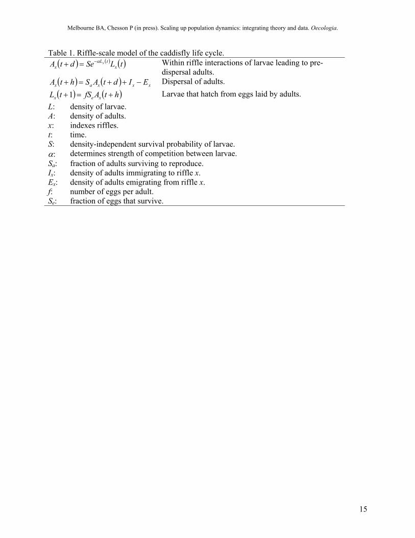
Table 1. Riffle-scale model of the caddisfly life cycle. ( ) ( ) ( )tLSedtA x

tLx

xα−=+ Within riffle interactions of larvae leading to pre-dispersal adults.

( ) ( ) xxxax EIdtAShtA −++=+ Dispersal of adults. ( ) ( )htAfStL xex +=+1 Larvae that hatch from eggs laid by adults.

L: density of larvae. A: density of adults. x: indexes riffles. t: time. S: density-independent survival probability of larvae. α: determines strength of competition between larvae. Sa: fraction of adults surviving to reproduce. Ix: density of adults immigrating to riffle x. Ex: density of adults emigrating from riffle x. f: number of eggs per adult. Se: fraction of eggs that survive.


16

Table 2. Parameter estimates, degrees of freedom, residual mean square, and Akaike information criterion for fits of the riffle-scale production function. Model Parameters d.f. r.m.s.a AIC True Ricker S = 0.70, α = 0.036 Ricker S = 0.669, α = 0.0345 38 0.01229 -26.5 Linear S = 0.306 39 0.2333 90.3 Beverton-Holt S = 1.033, c = 0.1187 38 0.02630 3.98 a Models were fitted on the natural logarithm scale.


17

Table 3. Analysis of variance summary for the variance components analysis of larval density showing degrees of freedom, sums of squares, mean squares, and variance components. Stratum d.f. s.s. m.s var. comp. Larvae Riffle 39 14492.215 371.595 181.431 Sample 40 349.337 8.733 8.733 Total 79 14841.552


18

L AA eggs L

t t+ht+d t+1S Sa Sef

Densitydependence Dispersal Reproduction Winter

Figure 1. Annual life cycle of the caddisfly (larvae L, adult A) showing times and parameters of the riffle-scale model (Table 1).


19

8

10000

T

T

T=0

Adu

lt de

nsity

, A(t+

d)

Larval density, L(t)

8

100

Mean-field model

Riffles y & z

yy z

y

z

z

a

b c

Figure 2. Nonlinear averaging with riffle-scale dynamics given by the Ricker model. The figure is for a simplified stream system that consists of just two riffles (y and z) with different densities of caddisfly larvae. Two different levels of spatial variation in larval density between riffles are represented in (a) (low variation) and (b) (high variation), holding mean density constant between (a) and (b). The survival of larvae through to adults is density dependent according to the Ricker model (thick curve) in (a) and (b) and density independent (thick line) in (c). The dashed lines connect the larval densities (L(t)) in each riffle with the density of adults (A(t+d)) that emerge from each riffle. The solid line connects the average larval density of the two riffles with the density of emerging adults that would be expected if larval density in the stream was homogeneous (mean field). Nonlinear averaging (a and b) occurs when there is spatial variation in larval density because the density of adults emerging from the stream is the average (○) of the output from the two riffles (dashed lines). The magnitude of the scale transition (T) is the difference between the spatial average (○) and the mean-field (●). When there is more variation between riffles (b) the scale transition is greater. When local dynamics are linear, there is no scale transition (c).


20

a

c

e

b

d

f

0

40

80

120

0

15

30

45

0

40

80

120

0

15

30

45

0 10 20 30

-5

0

5

10

0 10 20 30

-5

-3

-1

1

3

Time

LL x

T,V

ar(L

)/100

High R Low R

Mean-field model

Spatial simulation

Var(L(t))

T

T approx

Fig. 3. One realization of the spatial simulation with the negative binomial dispersal model for high (left column) and low (right column) values of the density-independent finite rate of increase R (R = S Sa f Se,). a, b) The mean density of larvae from the 1000 riffles in the stream (closed circles) compared with riffle-scale dynamics in the absence of migration (or mean-field model; open circles). c, d) The dynamics of density in three of the 1000 riffles. Each symbol represents a different riffle. e, f) The dynamics of the spatial variance in larval density, Var(L(t)), (squares), and the scale transition, T, measured (i) by the quadratic approximation (Eq. 9, 12) (crosses), and (ii) exactly by the difference in production between the spatial simulation and the mean-field model (i.e. Eq. 7) (open circles). Var(L) is the population variance of the 1000 riffles. a, c, e) α = 0.036, R = 8.75 (S = 0.7, f = 25, SaSe = 0.5), k = 5. b, d, f) α = 0.036, R = 2.625 (S = 0.7, f = 25, SaSe = 0.15), k = 3.


21

0 30 60 900

30

60

90

0 30 60 900

10

20

L (t)

L (t

+ 1)

a b

Fig. 4. Production functions for the mean field (Ricker) model (solid line) compared to points from one realization of the spatial simulation with the negative binomial dispersal model (open circles) for high (a) and low (b) values of the density-independent finite rate of increase R (R = S Sa f Se,). The exact scale transition (Eq. 7) is the vertical difference between the mean field curve and each point. The quadratic approximation (Eq. 14) is also shown (crosses). Overlapping points were removed for clarity. The dashed line is the stream-scale production function: the theoretical expectation of the Ricker model with negative binomial variation (Chesson 1996; De Jong 1979); this curve is a check on the simulation results and shows the full effect of scaling up on the production function. a) α = 0.036, R = 8.75 (S = 0.7, f = 25, SaSe = 0.5), k = 5. b) α = 0.036, R = 2.625 (S = 0.7, f = 25, SaSe = 0.15), k = 3.


22

0 20 40 600

3

6

9

L(t)

A(t+

d)

Fig. 5. Different models for the riffle-scale production function fitted to simulated data. The best fitting model was the Ricker model (solid line) which can be compared with the Beverton-Holt model (dashes) and a linear model (dots - dashes).

Documents

Scaling up population dynamics: integrating theory and …€¦Melbourne BA, Chesson P (in press). Scaling up population dynamics: integrating theory and data. Oecologia. 2 Abstract