Scheduling a Single Machine to Minimize a Regular ...baptiste/do04.pdf · Scheduling a Single Machine to Minimize a Regular Objective Function under Setup Constraints ... a Branch

Scheduling a Single Machine to Minimize a

Regular Objective Function under Setup

Constraints

Philippe Baptiste a Claude Le Pape b

aCNRS LIX, Ecole Polytechnique, F-91128, Palaiseau,[email protected]

bILOG, Gentilly, France, [email protected]

Abstract

Motivated by industrial applications, we study the scheduling situation in which aset of jobs subjected to release dates and deadlines are to be performed on a singlemachine. The objective is to minimize a regular sum objective function

∑i fi where

fi(Ci) corresponds to the cost of the completion of job Ji at time Ci. On top of this,we also take into account setup times and setup costs between families of jobs as wellas the fact that some jobs can be “unperformed” to reduce the load of the machine.We introduce lower bounds and dominance properties for this problem and wedescribe a Branch and Bound procedure with constraint propagation. Experimentalresults are reported.

Key words: Single Machine Scheduling; Sequencing; Setup Time; Setup Cost;Unperformed Jobs

1 Introduction

Real manufacturing scheduling problems exhibit a number of difficult featuresthat are often ignored in the literature. Motivated by a new testbed inspiredby industrial real life situations [29], we study in this paper the one machinescheduling problem with:

• Release dates and deadlines.• Costs dependent on the completion times of activities.• Possibilities of leaving some jobs “unperformed.”• Setup times and costs.

Preprint submitted to Elsevier Science 5 January 2005

In this problem, a set of jobs {J1, ..., Jn} subjected to release dates ri anddeadlines di are to be performed on a single machine. The processing timeof Ji is pi. The objective is to minimize a regular (i.e., non-decreasing) sumobjective function

∑i fi where fi(Ci) corresponds to the cost of completing Ji

at time Ci ∈ [ri + pi, di]. Two extensions of this core problem are considered:

• When the machine is overloaded some jobs can be “unperformed” to reducethe machine load. In such a case, an “unperformance” cost ui is associatedto each job Ji. When the job is not scheduled in its time window [ri, di],the cost ui is added to the objective function. Note that if the fi functionsare null, the problem reduces to minimizing

∑wiUi, a well-known objective

function in scheduling theory (see for instance, [10]). This additional costcan be integrated in the cost functions fi. Note however than when non-performance costs are used, fi is constant over the interval (di,∞) and theexact completion time of job Ji is no longer relevant once it is known toexceed di.• Due to manufacturing constraints, setups must be performed between jobs

with different machine feature requirements. We rely on the following model:there are q families of jobs and φ(Ji) ∈ {1, ..., q} denotes the family of thejob Ji. Within the same family, there is no transition time nor cost. Butbetween consecutive jobs of families φ1 and φ2, at least δ(φ1, φ2) units oftime must elapse. Moreover, a cost f(φ1, φ2) is associated to this setup.

We describe a new lower bound for this very general problem and a Branchand Bound procedure with constraint propagation. Experimental results arereported.

1.1 Literature Review

A lot of research has been carried on the unweighted total tardiness problemwith equal release dates 1||∑Ti. Powerful dominance rules have been in-troduced by Emmons [23]. Lawler [27] has proposed a dynamic programmingalgorithm that solves the problem in pseudo-polynomial time. Finally, Du andLeung have shown that the problem is NP-Hard [22]. Most of the exact meth-ods for solving 1||∑ Ti strongly rely on Emmons’ dominance rules. Potts andVan Wassenhove [30], Chang et al.[14] and Szwarc et al.[40], have developedBranch and Bound methods using the Emmons rules coupled with the decom-position rule of Lawler [27] together with some other elimination rules. Thebest results have been obtained by Szwarc, Della Croce and Grosso [40, 41]with a Branch and Bound method that efficiently handles instances with upto 500 jobs. The weighted problem 1||∑ wiTi is strongly NP-Hard [27]. Forthis problem, Rinnooy Kan et al.[35] and Rachamadugu [31] have extendedthe Emmons Rules [23]. Exact approaches based on Dynamic Programing and

2

Branch and Bound have been tested and compared by Abdul-Razacq, Pottsand Van Wassenhove [1].

There are less results on the problem with arbitrary release dates 1|ri|∑ Ti.Chu and Portmann [18] have introduced a sufficient condition for local opti-mality which allows them to build a dominant subset of schedules. Chu [16] hasalso proposed a Branch and Bound method using efficient dominance rules.This method handles instances with up to 30 jobs for the hardest instancesand with up to 230 jobs for the easiest ones. More recently, Baptiste, Carlierand Jouglet [4] have described a new lower bound and some dominance ruleswhich are used in a Branch and Bound procedure which handles instances withup to 50 jobs for the hardest instances and 500 jobs for the easiest ones. Letus also mention that exact Branch and Bound procedures have been proposedfor the same problem with setup times [32, 38]. For the 1|ri|∑ wiTi prob-lem, Akturk and Ozdemir [3] have proposed a sufficient condition for localoptimality which improves heuristic algorithms. This rule is then used with ageneralization of Chu’s dominance rules to the weighted case in a Branch andBound algorithm [2]. This Branch and Bound method handles instances withup to 20 jobs. Recently Jouglet et al. [25] have proposed a new Branch andBound that solves all instances with up to 35 jobs.

For the total completion time problem, in the case of identical release dates,both the unweighted and the weighted problems 1||∑wiCi can easily besolved polynomially in O(n log n) by applying the Shortest Weighted Pro-cessing Time priority rule, also called Smith’s rule [37]. For the unweightedproblem with release dates, several researchers have introduced dominanceproperties and proposed a number of algorithms [13, 21, 20]. Chu [15, 17] hasproved several dominance properties and has provided a Branch and Boundalgorithm. Chand, Traub and Uzsoy used a decomposition approach to im-prove Branch and Bound algorithms [12]. Among the exact methods, the mostefficient algorithms [15, 12] can handle instances with up to 100 jobs. Theweighted case with release dates 1|ri|∑ wiCi is NP-Hard in the strong sense[34] even when the preemption is allowed [26]. Several dominance rules andBranch and Bound algorithms have been proposed [8, 9, 24, 33]. To our kn-woledge, the best results are obtained by Belouadah, Posner and Potts witha Branch and Bound algorithm which has been tested on instances involvingup to 50 jobs.

Many exact methods have been proposed for the problem 1|ri|∑Ui [5, 19, 7].More recently, Ruslan Sadykov [36] has proposed a very efficient Branch andCut algorithm for this problem.

3

1.2 Overall Framework

Our Branch and Bound has been implemented in a Constraint Programmingframework. Constraint Programming is a paradigm aimed at solving combi-natorial optimization problems. Often these combinatorial optimization prob-lems are solved by defining them as one or several instances of the ConstraintSatisfaction Problem (CSP). Informally speaking, an instance of the CSP isdescribed by a set of variables, a set of possible values for each variable, anda set of constraints between the variables. The set of possible values of a vari-able is called the variable’s domain. A constraint between variables expresseswhich combinations of values for the variables are allowed. Constraints can bestated either implicitly (intentionally), e.g., an arithmetic formula, or explic-itly (extensionally), where each constraint is expressed as a set of tuples ofvalues that satisfy the constraint. The question to be answered for an instanceof the CSP is whether there exists an assignment of values to variables, suchthat all constraints are satisfied. Such an assignment is called a solution of theCSP.

One of the key ideas of constraint programming is that constraints can beused “actively” to reduce the computational effort needed to solve combina-torial problems. Constraints are thus not only used to test the validity ofa solution, as in conventional programming languages, but also in an activemode to remove values from the domains, deduce new constraints, and detectinconsistencies. This process of actively using constraints to come to certaindeductions is called constraint propagation. The specific deductions that resultin the removal of values from the domains are called domain reductions. Theset of values in the domain of a variable that are not invalidated by constraintpropagation is called the current domain of that variable.

As the general CSP is NP-complete constraint propagation is usually incom-plete. This means that some but not all the consequences of the set of con-straints are deduced. In particular, constraint propagation cannot detect allinconsistencies. Consequently, one needs to perform some kind of search todetermine if the CSP instance at hand has a solution or not. Most commonly,search is performed by means of a tree search algorithm.

We associate a start variable Si to each job Ji. Its domain is initially set to[ri, di− pi]. Throughout the search, the domains of start variables change butto keep things simple, we denote by ri the minimum value in the domain of Si

and by di the maximum value in Si plus pi. To model the objective function,we add a variable F to the model. It is constrained to be equal to the valueof the objective function.

F =∑

i

fi(Si + pi) (1)

4

To propagate the above constraint, we rely on Arc-B-consistency [28], (i.e.,Arc-consistency restricted to the bounds of the domains of the variables).Given a constraint c over n variables x1, . . . , xn and a domain d(xi) = [lb(xi), ub(xi)]for each variable xi, c is said to be “arc-B-consistent” if and only if for anyvariable xi and each of the bound values vi = lb(xi) and vi = ub(xi), thereexist values v1, . . . , vi−1, vi+1, . . . , vn in d(x1), . . . , d(xi−1), d(xi+1), . . . , d(xn)such that c(v1, . . . , vn) holds. Arc-B-consistency can be easily achieved on (1)since the fi functions are non-decreasing.

To propagate the resource constraints, we use the disjunctive constraint andthe edge-finding mechanism, as implemented in Ilog Scheduler [6]. It con-sists in determining whether an activity must, can, or cannot be the first or thelast to execute among a set of activities that require the same machine [11].This mechanism provides tightened time bounds for activities requiring thesame machine. It is known to be extremely powerful and can be implementedin O(n logn).

Once all constraints of the problem are added, a common technique to lookfor an optimal solution is to solve successive decision variants of the problem.Several strategies can be considered to minimize the value of F . One way is toiterate on the possible values, either from the lower bound of its domain up tothe upper bound until one solution is found, or from the upper bound down tothe lower bound determining each time whether there still is a solution. An-other way is to use a dichotomizing algorithm, where one starts by computingan initial upper bound ub and an initial lower bound lb for F . Then

(1) Set D =

⌊lb + ub

2

⌋

(2) Constrain F to be at most D. Then solve the resulting CSP, i.e., deter-mine a solution with F ≤ D or prove that no such solution exists. If asolution is found, set ub to the value of F in the solution; otherwise, setlb to D + 1.

(3) Iterate steps 1 and 2 until ub = lb.

We rely on the edge-finding branching scheme (see for instance [11]). Ratherthan searching for the starting times of jobs, we look for a sequence of jobs. Thissequence is built both from the beginning and from the end of the schedule.Throughout the search tree, the status of a job changes. It can be marked as“ranked” (i.e., already scheduled at the begining or at the end of the sequence),or “unranked”. Among unranked jobs, a job is a “possible first” (last) if itcan be the first (last) one to execute among all unranked jobs. Conversely,some unranked jobs are marked as “non-possible first” (last). The status ofthe jobs is dynamically maintained throughout the search. The edge-findingrules detect immediately that some jobs can, cannot or must be the first toexecute in a sequence. Moreover, they maintain some consistency between the

5

scheduling data (release date, deadline) and the status of the jobs. Thanksto the edge-finding rules the number of “possible first” jobs is usually low ateach node of the search tree.

Our branching strategy is very simple : We select one job among the unrankedjobs that can be first and we make it precede all other unranked jobs. Uponbacktracking, this job is marked as “non-possible first” and another unrankedjob is chosen.

The heuristic used to select the job to schedule first is fairly difficult to setupsince we have arbitrary cost functions. Following preliminary experiments,we have decided to use the PRTT function of Chu and Portmann [18]. It hasbeen introduced for the single machine total tardiness problem and it has beenshown to be very efficient. If δi denotes the due date of Ji, PRTT (i) is thendefined as max(ri+pi, δi). In our case, we do not have a due date but we defineartificially one as the first time point t after ri such that fi(ri) < fi(t + 1).If fi is constant its due date is then set to the deadline di. Since fi functionsare arbitrary, it is very difficult to build reasonably good heuristics for theproblem. We believe that in concrete cases, our naive adaptation of PRTTworks rather well. The experimental evaluation of this heuristic is however notin the scope of the paper.

Finally, we use the “No Good Recording” technique, a simple and powerfultechnique to detect infeasible situations that have “almost” been encountered(see for instance [4]). Whenever it is known that the current partial sequencecannot be extended to a feasible schedule improving on the best-known so-lution, the characteristics of the partial sequence that make this extensionimpossible are recorded as a “No Good”. If later in the search these character-istics are encountered again, the corresponding node is immediately discarded.

In our algorithm, we save:

• the set of jobs belonging to the partial sequence (recall that the schedule isbuilt from left to right);• the completion time of the last job in the partial sequence;• and the cost associated to the partial sequence.

If later in the search tree there exists a “No Good” including the currentpartial sequence, with a smaller (or equal) completion time and a smaller (orequal) total cost, then we immediately backtrack. Indeed, the partial sequenceat the current node cannot be extended to an improving complete schedule,since otherwise the “No Good” could have been extended to an improvingcomplete schedule.

6

2 Lower Bound

In this section and in Section 3, we assume that jobs cannot be left unper-formed and are not subjected to setup times and costs. We also assume thatthe cost functions are defined at any time point (i.e., before ri + pi and afterthe deadline). If this is not the case we can extend a function fi as follows∀t ≤ ri + pi, fi(t) = fi(ri + pi) and ∀t ≥ di, fi(t) = fi(di). The lower bound iscomputed in two steps:

step 1 First we compute a vector (C[1], C[2], ..., C[n]) such that ∀i, C[i] is a lowerbound of the ith smallest completion time in any schedule.

step 2 Second we define an assignment problem between jobs and the above com-pletion times C[1], C[2], ..., C[n]. The cost of assigning the job Ji to the dateC[u] is fi(C[u]) and we seek to minimize the total assignment cost.

Note that if the functions fi were not regular (non-decreasing), the optimalassignment cost would not be a lower bound because optimal schedules wouldnot be left shifted.

To achieve the first step, we allow preemption and jobs are scheduled accord-ing to the SRPT (Shortest Remaining Processing Time) rule: Each time ajob becomes available or is completed, a job with the shortest remaining pro-cessing time among the available and uncompleted jobs is scheduled. It is wellknown that the completion times C[1], C[2], ..., C[n] obtained on this preemptiveschedule are minimal, i.e., ∀i, C[i] is a lower bound of the completion time ofthe i-th job in any preemptive schedule. Using heap structures, the preemp-tive SRPT schedule can be build in O(n log n). This first step is a straightadaptation of Chu’s lower bound for 1|ri|∑ Ti.

The second step is a simple assignment problem and the Hungarian algorithmcould be used to compute an optimal solution in cubic time. As we wish to usethis lower bound in a Branch and Bound procedure, we propose to compute afast lower bound of the assignment problem. It is possibly not as good as theoptimal assignment value but is computed much faster. In the following, werely on the fact that the fi functions are non-decreasing.

Our basic observation is that, since the fi functions are non-decreasing andsince C[1] ≤ C[2] ≤ ... ≤ C[n], the total assignment cost is at least

n∑i=1

fi(C[1]).

7

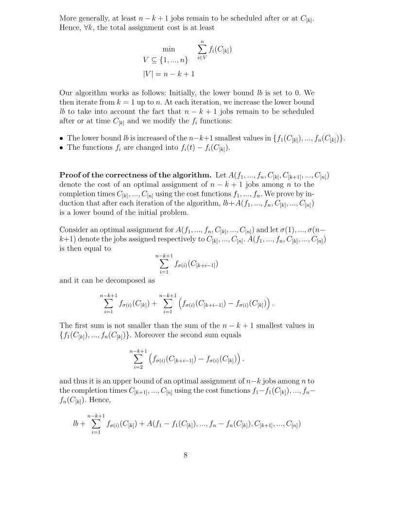
More generally, at least n− k + 1 jobs remain to be scheduled after or at C[k].Hence, ∀k, the total assignment cost is at least

min

V ⊆ {1, ..., n}|V | = n− k + 1

n∑i∈V

fi(C[k])

Our algorithm works as follows: Initially, the lower bound lb is set to 0. Wethen iterate from k = 1 up to n. At each iteration, we increase the lower boundlb to take into account the fact that n − k + 1 jobs remain to be scheduledafter or at time C[k] and we modify the fi functions:

• The lower bound lb is increased of the n−k+1 smallest values in {f1(C[k]), ..., fn(C[k])}.• The functions fi are changed into fi(t)− fi(C[k]).

Proof of the correctness of the algorithm. Let A(f1, ..., fn, C[k], C[k+1], ..., C[n])denote the cost of an optimal assignment of n − k + 1 jobs among n to thecompletion times C[k], ..., C[n] using the cost functions f1, ..., fn. We prove by in-duction that after each iteration of the algorithm, lb+A(f1, ..., fn, C[k], ..., C[n])is a lower bound of the initial problem.

Consider an optimal assignment for A(f1, ..., fn, C[k], ..., C[n]) and let σ(1), ..., σ(n−k+1) denote the jobs assigned respectively to C[k], ..., C[n]. A(f1, ..., fn, C[k], ..., C[n])is then equal to

n−k+1∑i=1

fσ(i)(C[k+i−1])

and it can be decomposed as

n−k+1∑i=1

fσ(i)(C[k]) +n−k+1∑

i=1

(fσ(i)(C[k+i−1])− fσ(i)(C[k])

).

The first sum is not smaller than the sum of the n− k + 1 smallest values in{f1(C[k]), ..., fn(C[k])}. Moreover the second sum equals

n−k+1∑i=2

(fσ(i)(C[k+i−1])− fσ(i)(C[k])

).

and thus it is an upper bound of an optimal assignment of n−k jobs among n tothe completion times C[k+1], ..., C[n] using the cost functions f1−f1(C[k]), ..., fn−fn(C[k]). Hence,

lb +n−k+1∑

i=1

fσ(i)(C[k]) + A(f1 − f1(C[k]), ..., fn − fn(C[k]), C[k+1], ..., C[n])

8

is also a lower bound of the initial problem.

A major weakness of the above lower bound is that release dates are takeninto account in the first step (computation of the earliest possible completiontimes) but not in the second one (assignment). Consider a 2-job instance withJ1 (r1 = 0, p1 = 2, d1 = 4, f1(2) = f1(3) = f1(4) = 0) and J2 (r2 = 1, p2 =2, d2 = 4, f2(3) = 0, f2(4) = 1). The completion time vector is (2, 4) and sincewe do not take into account release dates the optimal assignment is 0 whilethere is no feasible schedule with a cost lower than 1.

3 Dominance Properties

A dominance rule is a constraint that can be added to the initial problemwithout changing the value of the optimum, i.e., there is at least one optimalsolution of the problem for which the dominance holds. Dominance rules canbe of prime interest since they can be used to reduce the search space. Howeverthey have to be used with care since the optimum can be missed if conflictingdominance rules are combined.

In [4] we have introduced a set of dominance rules for 1|ri|∑ Ti that generalizeand extend Emmons rules [23]. Unfortunately, in the context of arbitrary non-decreasing objective functions, we have very little information available and itis rather difficult to generalize such rules. We propose a very simple set of ruleswhich allow us to add precedences between jobs. As we will see in Section 5,adding such precedences tightens the problem, increases the lower bound andhence improves our search procedure.

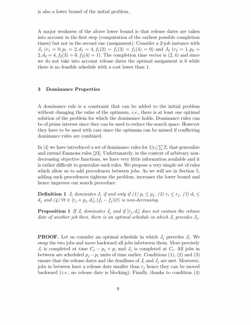
Definition 1 Ji dominates Jj if and only if (1) pi ≤ pj, (2) ri ≤ rj, (3) di ≤dj and (4) ∀t ∈ [rj + pj, di], (fi − fj)(t) is non-decreasing.

Proposition 1 If Ji dominates Jj and if [rj, di] does not contain the releasedate of another job then, there is an optimal schedule in which Ji precedes Jj.

PROOF. Let us consider an optimal schedule in which Jj precedes Ji. Weswap the two jobs and move backward all jobs inbetween them. More preciselyJi is completed at time Cj − pj + pi and Jj is completed at Ci. All jobs inbetween are scheduled pj−pi units of time earlier. Conditions (1), (2) and (3)ensure that the release dates and the deadlines of Ji and Jj are met. Moreover,jobs in between have a release date smaller than rj hence they can be movedbackward (i.e., no release date is blocking). Finally, thanks to condition (4)

9

and because the fu functions are regular, the cost of the resuting schedule isat least as good as the inital one.

Proposition 1 is used as a dominance rule at each node of the search tree.To apply the corresponding rule, the most time-consuming part is to checkif condition (4) holds or not. Most often the functions are piecewise linearfunctions and thus the tests can be easily implemented in time proportionalto the number of linear pieces. When two such jobs Ji, Jj are detected, weadjust release dates and deadlines as follows : rj ← max(rj , ri + pi) and di ←min(di, dj − pj).

4 Extensions

Following the requirements of ILOG’s customers, two kind of extensions havebeen considered. First, it often happens that machines of the shop floor be-come overloaded and thus some jobs Ji cannot be performed within their timewindow [ri, di]. Some jobs must then be left “unperformed”. Second, setuptimes and setup costs have to be taken into account.

4.1 Unperfomed Jobs

Unperformed jobs can be easily modeled within our initial framework. Indeed,we can set the deadline di to ∞ and change the function fi into f ′

i so that fort ≤ di, f ′

i(t) = fi(t), and for t ≥ di, f ′i(t) = ui. Provided this change is made,

the unperformed jobs are now performed very late and it is easy to see thatthe models are equivalent.

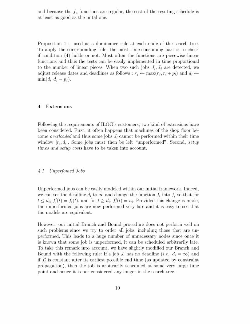
However, our initial Branch and Bound procedure does not perform well onsuch problems since we try to order all jobs, including those that are un-performed. This leads to a huge number of unnecessary nodes since once itis known that some job is unperformed, it can be scheduled arbitrarily late.To take this remark into account, we have slightly modified our Branch andBound with the following rule: If a job Ji has no deadline (i.e., di = ∞) andif f ′

i is constant after its earliest possible end time (as updated by constraintpropagation), then the job is arbitrarily scheduled at some very large timepoint and hence it is not considered any longer in the search tree.

10

4.2 Setup Times, Setup Costs

4.2.1 Constraint Propagation

We rely on the Ilog Scheduler mechanism to take into account setup timesand costs. For each job Ji, a lower bound on the setup time and cost betweenits (unknown) predecessor Jj and Ji is maintained, depending on the possiblepredecessors of Ji. Note that when Ji is ranked, its predecessor Jj is exactlyknown, and the setup time and cost consequently set to their exact values.When setup times satisfy the triangle inequality, Arc-B-consistency is alsoachieved on the disjunctive constraint

Si + pi + δ(φ(Ji), φ(Jj)) ≤ Sj or Sj + pj + δ(φ(Jj), φ(Ji)) ≤ Si.

4.2.2 Lower Bound

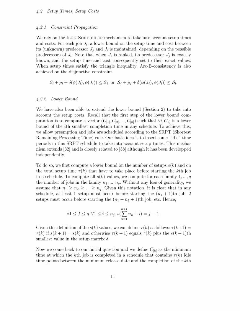
We have also been able to extend the lower bound (Section 2) to take intoaccount the setup costs. Recall that the first step of the lower bound com-putation is to compute a vector (C[1], C[2], ..., C[n]) such that ∀i, C[i] is a lowerbound of the ith smallest completion time in any schedule. To achieve this,we allow preemption and jobs are scheduled according to the SRPT (ShortestRemaining Processing Time) rule. Our basic idea is to insert some “idle” timeperiods in this SRPT schedule to take into account setup times. This mecha-nism extends [32] and is closely related to [38] although it has been developpedindependently.

To do so, we first compute a lower bound on the number of setups s(k) and onthe total setup time τ(k) that have to take place before starting the kth jobin a schedule. To compute all s(k) values, we compute for each family 1, ..., qthe number of jobs in the family n1, ..., nq. Without any loss of generality, weassume that n1 ≥ n2 ≥ ... ≥ nq. Given this notation, it is clear that in anyschedule, at least 1 setup must occur before starting the (n1 + 1)th job, 2setups must occur before starting the (n1 + n2 + 1)th job, etc. Hence,

∀1 ≤ f ≤ q, ∀1 ≤ i ≤ nf , s(u<f∑u=1

nu + i) = f − 1.

Given this definition of the s(k) values, we can define τ(k) as follows: τ(k+1) =τ(k) if s(k + 1) = s(k) and otherwise τ(k + 1) equals τ(k) plus the s(k + 1)thsmallest value in the setup matrix δ.

Now we come back to our initial question and we define C[k] as the minimumtime at which the kth job is completed in a schedule that contains τ(k) idletime points between the minimum release date and the completion of the kth

11

job. Given this definition of C[k], it is easy to see that in an optimal schedule(for C[k]), all jobs can be shifted to the right so that we have no idle time oncethe first job has started. Hence, we can compute C[k] as follows: (1) Wait τ(k)units of time from the minimum release date mini ri up to mini ri + τ(k) and(2) apply the SRPT dispatching rule. The completion time of the kth job inthis schedule is optimal.

The above algorithm requires to run the SRPT dispatching rule each time anidle interval is inserted. Since there are at most q ≤ n distinct values of τ(k),no more than q SRPT schedules are relevant. Each SRPT schedule can becomputed in O(n logn), hence the overall complexity is O(qn logn).

4.2.3 Dominance Properties

The dominance rule proposed in Section 3 is easy to extend to jobs in thesame family.

Proposition 2 If Ji dominates Jj, if [rj + pj, di] does not contain a releasedate and if Ji and Jj belong to the same family then, there is an optimalschedule in which Ji precedes Jj.

4.2.4 No Good Recording

The situation is slightly more complex since the family of the last job in apartial sequence has an impact on the remaining jobs. So, on top of the set ofjobs, the completion time of the last job and the cost associated to the partialsequence, we also store the family of the last job in the sequence. The “NoGood” test then works as follows: If later in the search tree we have a partialsequence including the same set of jobs as in the No Good sequence that doesnot improve the completion time of its last job nor its total cost and if thefamily of the last job in the No Good sequence is the same as the family ofthe last job in the current sequence then we immediately backtrack.

5 Experimental Results

We have tested four variants of our Branch and Bound algortihm:

• Either we use the lower bound (LB) or not (NO-LB) and• either we use the No Good Recording (NG) technique or not (NO-NG).

We have run our tests on several instances from the Manufacturing SchedulingLibrary (MaScLib) [29] available at www2.ilog.com/masclib. These instances

12

are inspired by industrial real life situations and they have been made availableto the research community to facilitate manufacturing scheduling research byproviding an industrial basis to test scheduling algorithms and through thatincrease overall interest in manufacturing scheduling research. NCOS instancesassume no setup while STC NCOS instances assume setup times and costs. Twovariants have been considered: In the first one all activities have to be per-formed while in the other one, activities can be unperformed. The instanceswe have considered are the ones in which the overall objective to minimize isthe sum of processing costs, setup costs, tardiness costs (with respect to idealdue-dates), and non-performance costs, as defined in [29]. Our Branch andBound algortihm does not apply to MaScLib instances with earliness costs, asearliness costs lead to non-regular cost functions.

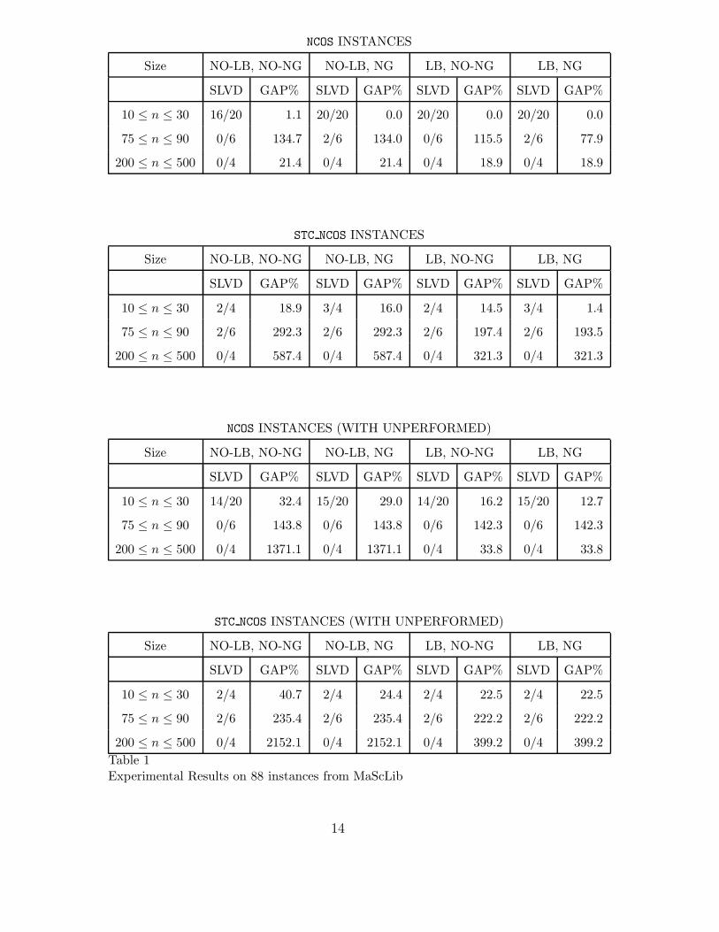
Instances have been grouped according to their size and for each group, wehave reported the number of instances solved among all instances of the group(SLVD) and the average relative GAP% between the upper bound and thelower bound when the search is stopped, i.e., either when the optimal solutionis found or after 30 minutes of CPU time on a 1.4 GHz PC running WindowsXP.

The combination of the lower bound and of the No Good Recording provesto be very useful both in terms of number of instances solved and of gapreduction. To further evaluate the effect of LB and NG we report in Table 2the average CPU time and the average number of backtracks for instances ofthe problem that are solved by all versions of our Branch and Bound procedure.

Few instances of the MaScLib have a special structure (no deadline, no setup,no unperformed jobs, simple objective functions) and hence they can be con-sidered as instances of 1|ri|∑ wiTi. For this later problem Jouglet has pro-posed a very efficient Branch and Bound procedure [25] that incorporateslower bounds, strong dominance properties and specific branching strategiesthat we cannot use in our general Branch and Bound. Still, we have beenable to compare the efficiency of the two procedures. Among 30 instances, ourprocedure is able to solve 22 of them that are also solved by Jouglet’s specificprocedure. However we need, on the average, 30 seconds of CPU time and1707 backtracks while Jouglet’s procedure requires 3 seconds and 215 back-tracks only. Also note that, within 30 minutes, two more instances are solvedby Jouglet. As mentioned earlier, our Branch and Bound tackles a much morecomplex problem than 1|ri|∑ wiTi so the fact that it does not perform as wellas specific techniques is not very surprising.

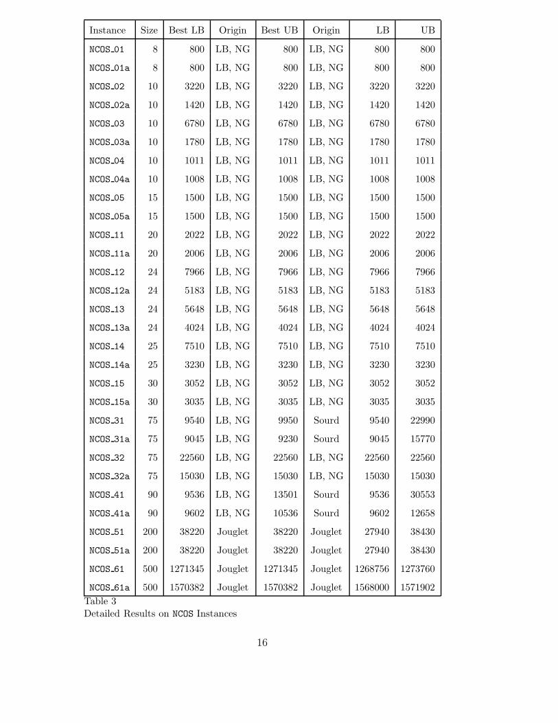
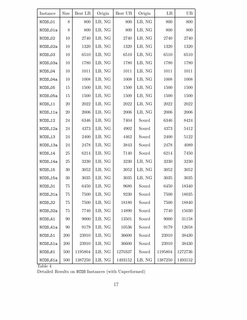
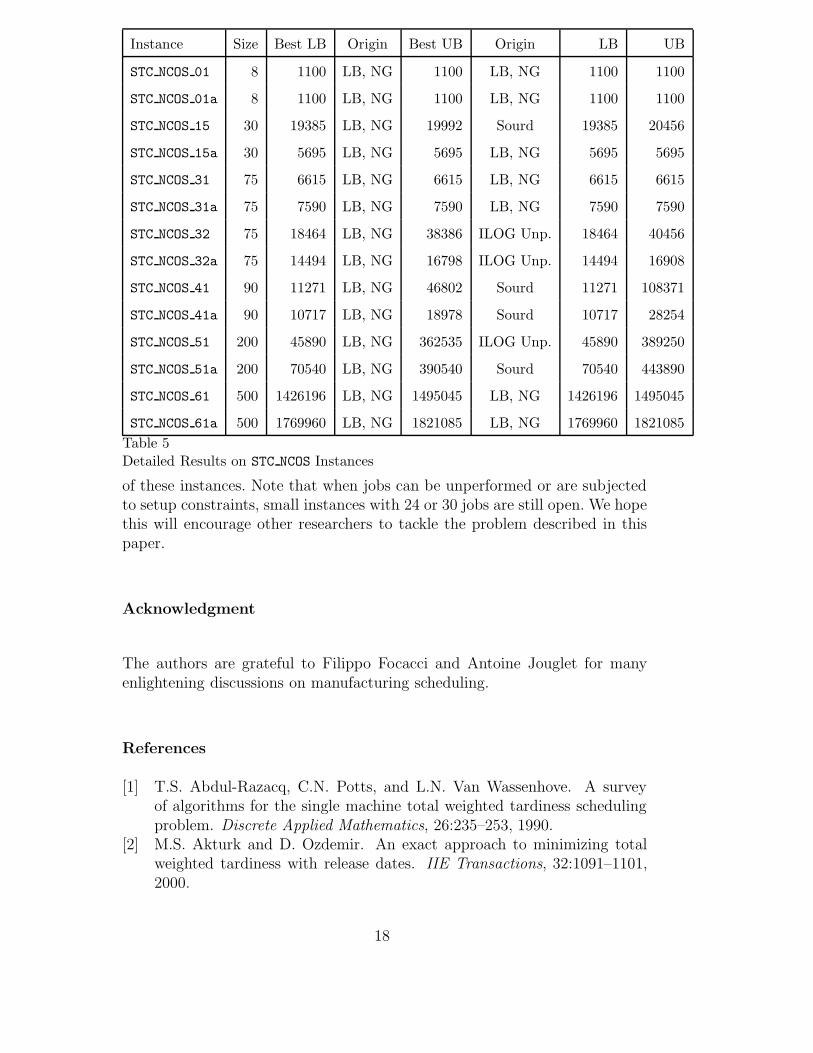
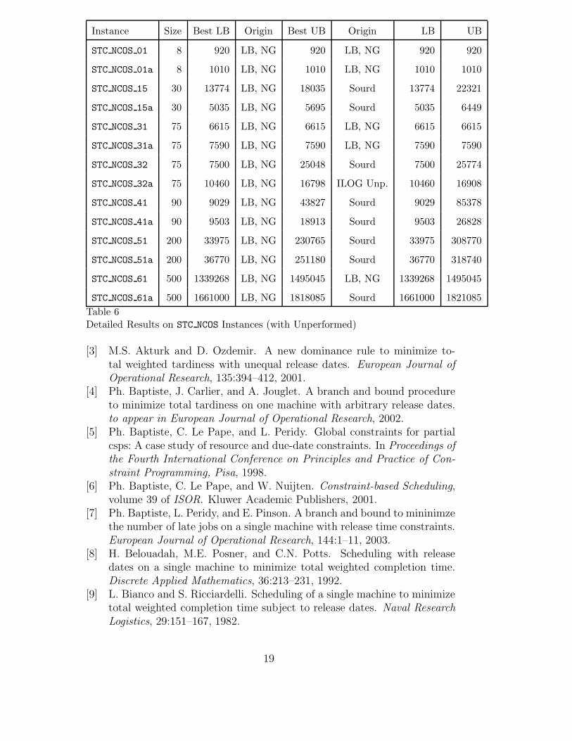
Tables 3, 4, 5 and 6 provide detailed results. For each instance, the tablesprovide the best-known lower bound (Best LB), the best known upper bound(Best UB), and the lower and upper bounds (LB and UB) provided by ourBranch and Bound with lower bounds and nogoods. The tables also provide

13

NCOS INSTANCES

Size NO-LB, NO-NG NO-LB, NG LB, NO-NG LB, NG

SLVD GAP% SLVD GAP% SLVD GAP% SLVD GAP%

10 ≤ n ≤ 30 16/20 1.1 20/20 0.0 20/20 0.0 20/20 0.0

75 ≤ n ≤ 90 0/6 134.7 2/6 134.0 0/6 115.5 2/6 77.9

200 ≤ n ≤ 500 0/4 21.4 0/4 21.4 0/4 18.9 0/4 18.9

STC NCOS INSTANCES



10 ≤ n ≤ 30 2/4 18.9 3/4 16.0 2/4 14.5 3/4 1.4

75 ≤ n ≤ 90 2/6 292.3 2/6 292.3 2/6 197.4 2/6 193.5

200 ≤ n ≤ 500 0/4 587.4 0/4 587.4 0/4 321.3 0/4 321.3

NCOS INSTANCES (WITH UNPERFORMED)



10 ≤ n ≤ 30 14/20 32.4 15/20 29.0 14/20 16.2 15/20 12.7

75 ≤ n ≤ 90 0/6 143.8 0/6 143.8 0/6 142.3 0/6 142.3

200 ≤ n ≤ 500 0/4 1371.1 0/4 1371.1 0/4 33.8 0/4 33.8

STC NCOS INSTANCES (WITH UNPERFORMED)



10 ≤ n ≤ 30 2/4 40.7 2/4 24.4 2/4 22.5 2/4 22.5

75 ≤ n ≤ 90 2/6 235.4 2/6 235.4 2/6 222.2 2/6 222.2

200 ≤ n ≤ 500 0/4 2152.1 0/4 2152.1 0/4 399.2 0/4 399.2Table 1Experimental Results on 88 instances from MaScLib

14

NO-LB, NO-NG NO-LB, NG LB, NO-NG LB, NG

CPU BCK CPU BCK CPU BCK CPU BCK

NCOS (No Unp.) 6.3 5632 2.9 1332 20.1 5632 9.9 1332

STC NCOS (No Unp.) 0.4 974 0.2 144 0.6 774 0.3 127

NCOS (Unp.) 0.7 1763 0.1 161 0.6 1276 0.1 131

STC NCOS (Unp.) 172.3 72156 66.1 8391 186.9 71797 72.8 8388Table 2Average Number of Backtracks and Average CPU Time for instances solved by allversions of the Branch and Bound

the origin of the best known lower and upper bounds, i.e.:

• “LB,NG” for our Branch and Bound algorithm with lower bounds and no-goods;• “Jouglet” for the Branch and Bound algorithm presented in [25];• “Sourd” for the local search algorithm presented in [39];• “ILOG Unp.” for an unpublished constraint programming and local search

algorithm developed by T. Bousonville, F. Focacci and D. Godard at ILOG.

Our Branch and Bound algorithm provides the best-known lower bound for 82instances out of 88 and the best know upper bound for 50 instances. In manycases, however, the solutions found by other algorithms are much better thanthe solutions found by our Branch and Bound. This reflects the fact that westill have to find good heuristics to explore the search space.

6 Conclusion

In this paper, we have presented a Branch and Bound procedure for the onemachine scheduling problem with:

• Release dates and deadlines.• Costs dependent on the completion times of activities.• Possibilities of leaving some jobs “unperformed”.• Setup times and costs.

To our knowledge, this is the first exact procedure for such a general problem.Further work includes the development of heuristics to more efficiently explorethe search space and the generalization of this procedure to more complexscheduling problems, e.g., to a multi-machine environment.

We tested our procedure on 88 instances of the Manufacturing SchedulingLibrary (MaScLib) [29], available at www2.ilog.com/masclib. We closed 46

15

Instance Size Best LB Origin Best UB Origin LB UB

NCOS 01 8 800 LB, NG 800 LB, NG 800 800

NCOS 01a 8 800 LB, NG 800 LB, NG 800 800

NCOS 02 10 3220 LB, NG 3220 LB, NG 3220 3220

NCOS 02a 10 1420 LB, NG 1420 LB, NG 1420 1420

NCOS 03 10 6780 LB, NG 6780 LB, NG 6780 6780

NCOS 03a 10 1780 LB, NG 1780 LB, NG 1780 1780

NCOS 04 10 1011 LB, NG 1011 LB, NG 1011 1011

NCOS 04a 10 1008 LB, NG 1008 LB, NG 1008 1008

NCOS 05 15 1500 LB, NG 1500 LB, NG 1500 1500

NCOS 05a 15 1500 LB, NG 1500 LB, NG 1500 1500

NCOS 11 20 2022 LB, NG 2022 LB, NG 2022 2022

NCOS 11a 20 2006 LB, NG 2006 LB, NG 2006 2006

NCOS 12 24 7966 LB, NG 7966 LB, NG 7966 7966

NCOS 12a 24 5183 LB, NG 5183 LB, NG 5183 5183

NCOS 13 24 5648 LB, NG 5648 LB, NG 5648 5648

NCOS 13a 24 4024 LB, NG 4024 LB, NG 4024 4024

NCOS 14 25 7510 LB, NG 7510 LB, NG 7510 7510

NCOS 14a 25 3230 LB, NG 3230 LB, NG 3230 3230

NCOS 15 30 3052 LB, NG 3052 LB, NG 3052 3052

NCOS 15a 30 3035 LB, NG 3035 LB, NG 3035 3035

NCOS 31 75 9540 LB, NG 9950 Sourd 9540 22990

NCOS 31a 75 9045 LB, NG 9230 Sourd 9045 15770

NCOS 32 75 22560 LB, NG 22560 LB, NG 22560 22560

NCOS 32a 75 15030 LB, NG 15030 LB, NG 15030 15030

NCOS 41 90 9536 LB, NG 13501 Sourd 9536 30553

NCOS 41a 90 9602 LB, NG 10536 Sourd 9602 12658

NCOS 51 200 38220 Jouglet 38220 Jouglet 27940 38430

NCOS 51a 200 38220 Jouglet 38220 Jouglet 27940 38430

NCOS 61 500 1271345 Jouglet 1271345 Jouglet 1268756 1273760

NCOS 61a 500 1570382 Jouglet 1570382 Jouglet 1568000 1571902Table 3Detailed Results on NCOS Instances

16


NCOS 01 8 800 LB, NG 800 LB, NG 800 800

NCOS 01a 8 800 LB, NG 800 LB, NG 800 800

NCOS 02 10 2740 LB, NG 2740 LB, NG 2740 2740

NCOS 02a 10 1320 LB, NG 1320 LB, NG 1320 1320

NCOS 03 10 6510 LB, NG 6510 LB, NG 6510 6510

NCOS 03a 10 1780 LB, NG 1780 LB, NG 1780 1780

NCOS 04 10 1011 LB, NG 1011 LB, NG 1011 1011

NCOS 04a 10 1008 LB, NG 1008 LB, NG 1008 1008

NCOS 05 15 1500 LB, NG 1500 LB, NG 1500 1500

NCOS 05a 15 1500 LB, NG 1500 LB, NG 1500 1500

NCOS 11 20 2022 LB, NG 2022 LB, NG 2022 2022

NCOS 11a 20 2006 LB, NG 2006 LB, NG 2006 2006

NCOS 12 24 6346 LB, NG 7404 Sourd 6346 8424

NCOS 12a 24 4373 LB, NG 4902 Sourd 4373 5412

NCOS 13 24 2400 LB, NG 4462 Sourd 2400 5122

NCOS 13a 24 2478 LB, NG 3843 Sourd 2478 4089

NCOS 14 25 6214 LB, NG 7140 Sourd 6214 7450

NCOS 14a 25 3230 LB, NG 3230 LB, NG 3230 3230

NCOS 15 30 3052 LB, NG 3052 LB, NG 3052 3052

NCOS 15a 30 3035 LB, NG 3035 LB, NG 3035 3035

NCOS 31 75 6450 LB, NG 9680 Sourd 6450 18340

NCOS 31a 75 7500 LB, NG 9230 Sourd 7500 18035

NCOS 32 75 7500 LB, NG 18180 Sourd 7500 18840

NCOS 32a 75 7740 LB, NG 14890 Sourd 7740 15030

NCOS 41 90 9000 LB, NG 13501 Sourd 9000 31158

NCOS 41a 90 9179 LB, NG 10536 Sourd 9179 12658

NCOS 51 200 23910 LB, NG 36600 Sourd 23910 38430

NCOS 51a 200 23910 LB, NG 36600 Sourd 23910 38430

NCOS 61 500 1195804 LB, NG 1270337 Sourd 1195804 1272736

NCOS 61a 500 1387250 LB, NG 1493152 LB, NG 1387250 1493152Table 4Detailed Results on NCOS Instances (with Unperformed)

17


STC NCOS 01 8 1100 LB, NG 1100 LB, NG 1100 1100

STC NCOS 01a 8 1100 LB, NG 1100 LB, NG 1100 1100

STC NCOS 15 30 19385 LB, NG 19992 Sourd 19385 20456




STC NCOS 32 75 18464 LB, NG 38386 ILOG Unp. 18464 40456

STC NCOS 32a 75 14494 LB, NG 16798 ILOG Unp. 14494 16908


STC NCOS 41a 90 10717 LB, NG 18978 Sourd 10717 28254

STC NCOS 51 200 45890 LB, NG 362535 ILOG Unp. 45890 389250



STC NCOS 61a 500 1769960 LB, NG 1821085 LB, NG 1769960 1821085Table 5Detailed Results on STC NCOS Instances

of these instances. Note that when jobs can be unperformed or are subjectedto setup constraints, small instances with 24 or 30 jobs are still open. We hopethis will encourage other researchers to tackle the problem described in thispaper.

Acknowledgment

The authors are grateful to Filippo Focacci and Antoine Jouglet for manyenlightening discussions on manufacturing scheduling.

References

[1] T.S. Abdul-Razacq, C.N. Potts, and L.N. Van Wassenhove. A surveyof algorithms for the single machine total weighted tardiness schedulingproblem. Discrete Applied Mathematics, 26:235–253, 1990.

[2] M.S. Akturk and D. Ozdemir. An exact approach to minimizing totalweighted tardiness with release dates. IIE Transactions, 32:1091–1101,2000.

18









STC NCOS 32a 75 10460 LB, NG 16798 ILOG Unp. 10460 16908






STC NCOS 61a 500 1661000 LB, NG 1818085 Sourd 1661000 1821085Table 6Detailed Results on STC NCOS Instances (with Unperformed)

[3] M.S. Akturk and D. Ozdemir. A new dominance rule to minimize to-tal weighted tardiness with unequal release dates. European Journal ofOperational Research, 135:394–412, 2001.

[4] Ph. Baptiste, J. Carlier, and A. Jouglet. A branch and bound procedureto minimize total tardiness on one machine with arbitrary release dates.to appear in European Journal of Operational Research, 2002.

[5] Ph. Baptiste, C. Le Pape, and L. Peridy. Global constraints for partialcsps: A case study of resource and due-date constraints. In Proceedings ofthe Fourth International Conference on Principles and Practice of Con-straint Programming, Pisa, 1998.

[6] Ph. Baptiste, C. Le Pape, and W. Nuijten. Constraint-based Scheduling,volume 39 of ISOR. Kluwer Academic Publishers, 2001.

[7] Ph. Baptiste, L. Peridy, and E. Pinson. A branch and bound to mininimzethe number of late jobs on a single machine with release time constraints.European Journal of Operational Research, 144:1–11, 2003.

[8] H. Belouadah, M.E. Posner, and C.N. Potts. Scheduling with releasedates on a single machine to minimize total weighted completion time.Discrete Applied Mathematics, 36:213–231, 1992.

[9] L. Bianco and S. Ricciardelli. Scheduling of a single machine to minimizetotal weighted completion time subject to release dates. Naval ResearchLogistics, 29:151–167, 1982.

19

[10] Peter Brucker. Scheduling Algorithms. Springer, 2001.[11] J. Carlier and E. Pinson. A practical use of jackson’s preemptive schedule

for solving the job-shop problem. Annals of Operations Research, 26:269–287, 1990.

[12] S. Chand, R. Traub, and R. Uzsoy. Single-machine scheduling with dy-namic arrivals: Decomposition results and an improved algorithm. NavalResearch Logistics, 43:709–716, 1996.

[13] R. Chandra. On n/1/F dynamic determistic systems. Naval ResearchLogistics, 26:537–544, 1979.

[14] S. Chang, Q. Lu, Tang G., and W. Yu. On decomposition of the totaltardiness problem. Operations Research Letters, 17:221–229, 1995.

[15] C. Chu. A branch and bound algorithm to minimize total flow time withunequal release dates. Naval Research Logistics, 39:859–875, 1991.

[16] C. Chu. A branch and bound algorithm to minimize total tardiness withdifferent release dates. Naval Research Logistics, 39:265–283, 1992.

[17] C. Chu. Efficient heuristics to minimize total flow time with release dates.Operations Research Letters, 12:321–330, 1992.

[18] C. Chu and M.C. Portmann. Some new efficient methods to solve then|1|ri|∑ Ti scheduling problem. European Journal of Operational Re-search, 58:404–413, 1991.

[19] S. Dauzere-Peres and M. Sevaux. A branch and bound method to min-imize the number of late jobs on a single machine. Technical report,Research report 98/5/AUTO, Ecole des Mines de Nantes, 1998.

[20] D.S. Deogun. On scheduling with ready times to minimize mean flowtime. Comput. J., 26:320–328, 1983.

[21] M.I. Dessouky and D.S. Deogun. Sequencing jobs with unequal readytimes to minimize mean flow time. SIAM J. Comput., 10:192–202, 1981.

[22] J. Du and J.Y.T. Leung. Minimizing total tardiness on one processor isNP-Hard. Mathematics of Operations Research, 15:483–495, 1990.

[23] H. Emmons. One-machine sequencing to minimize certain functions ofjob tardiness. Operations Research, 17:701–715, 1969.

[24] A.M.A Hariri and C.N. Potts. An algorithm for single machine sequencingwith release dates to minimize total weighted completion time. DiscreteApplied Mathematics, 5:99–109, 1983.

[25] A. Jouglet, Ph. Baptiste, and J. Carlier. Handbook of Scheduling: Al-gorithms, Models and Performance Analysis, chapter Branch-and-BoundAlgorithms for Total Weighted Tardiness. CRC Press, 2004.

[26] J. Labetoulle, E.L. Lawler, J.K. Lenstra, and A.H.G Rinnooy Kan.Progress in Combinatorial Optimization, chapter Preemptive schedulingof uniform machines subject to release dates. Academic Press, New York,1984.

[27] E.L. Lawler. A pseudo-polynomial algorithm for sequencing jobs to min-imize total tardiness. Annals of Discrete Mathematics, 1:331–342, 1977.

[28] O. Lhomme. Consistency techniques for numeric CSPs. In Proceedings ofthe Thirteenth International Joint Conference on Artificial Intelligence,

20

1993.[29] W. Nuijten, T. Bousonville, F. Focacci, D. Godard, and C. Le Pape.

Towards an industrial manufacturing scheduling problem and test bed.In Proceedings of PMS’04, Nancy, 2004.

[30] C.N. Potts and L.N. Van Wassenhove. A decomposition algorithm forthe single machine total tardiness problem. Operations Research Letters,26:177–182, 1982.

[31] R.M.V. Rachamadugu. A note on weighted tardiness problem. OperationResearch, 35:450–452, 1987.

[32] G.L. Ragatz. A branch-and-bound method for minimum tardiness se-quencing on a single processor with sequence dependent setup times. InTwenty-fourth Annual Meeting of the Decison Sciences Institute, 1993.

[33] G. Rinaldi and A. Sassano. On a job scheduling problem with differentready time: Some properties and a new algorithm to determine the opti-mal solution. Operation Research, 1977. Rapporto dell’Ist. di Automaticadell’Universita di Roma e del C.S.S.C.C.A.-C.N.R.R, Report R.77-24.

[34] A.H.G. Rinnooy Kan. Machine sequencing problem: classification, com-plexity and computation. Nijhoff. The Hague, 1976.

[35] A.H.G. Rinnooy Kan, B.J Lageweg, and J.K. Lenstra. Minimizing totalcosts in one-machine scheduling. Operation Research, 23:908–927, 1975.

[36] R. Sadykov. A hybrid branch-and-cut algorithm for the one-machinescheduling problem. In Proceedings of the International Conference onIntegration of AI and OR Techniques in Constraint Programming forCombinatorial Optimisation Problems, 2004.

[37] W.E. Smith. Various optimizers for single stage production. Naval Re-search Logistics Quarterly, 3:59–66, 1956.

[38] A. Souissi, I. Kacem, and C. Chu. New lower bound for minimizing totaltardiness on a single machine with sequence-dependent setup times. InProceedings of the Ninth International Conference on Project Manage-ment and Scheduling, PMS04, 2004.

[39] F. Sourd. Earliness-tardiness scheduling with setup considerations. Com-puters & Operations Research, To appear.

[40] W. Szwarc, F. Della Croce, and A. Grosso. Solution of the single machinetotal tardiness problem. Journal of Scheduling, 2:55–71, 1999.

[41] W. Szwarc, A. Grosso, and F. Della Croce. Algorithmic paradoxes of thesingle machine total tardiness problem. Journal of Scheduling, 4:93–104,2001.

21

Documents

Scheduling a Single Machine to Minimize a Regular ...baptiste/do04.pdf · Scheduling a Single Machine to Minimize a Regular Objective Function under Setup Constraints ... a Branch